SPEED: Statically Estimating Symbolic Computational Complexity of

ProgramsSumit GulwaniMSR Redmond

Trishul ChilimbiMSR Redmond

Krishna MehraMSR Bangalore

Problem Definition

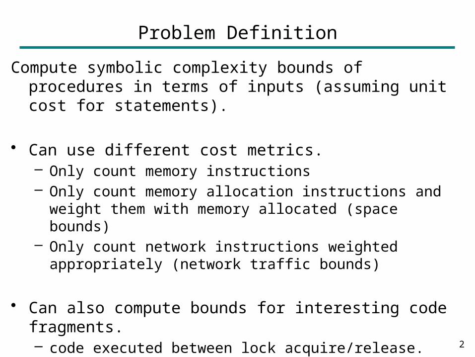
Compute symbolic complexity bounds of procedures in terms of inputs (assuming unit cost for statements).

• Can use different cost metrics.– Only count memory instructions– Only count memory allocation instructions and weight

them with memory allocated (space bounds)– Only count network instructions weighted appropriately

(network traffic bounds)

• Can also compute bounds for interesting code fragments.– code executed between lock acquire/release.

2

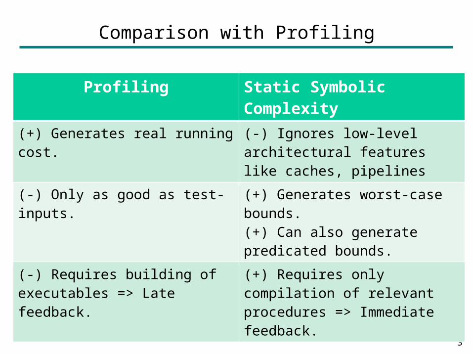
Comparison with Profiling

3

Profiling Static Symbolic Complexity

(+) Generates real running cost.

(-) Ignores low-level architectural features like caches, pipelines

(-) Only as good as test-inputs. (+) Generates worst-case bounds.(+) Can also generate predicated bounds.

(-) Requires building of executables => Late feedback.

(+) Requires only compilation of relevant procedures => Immediate feedback.

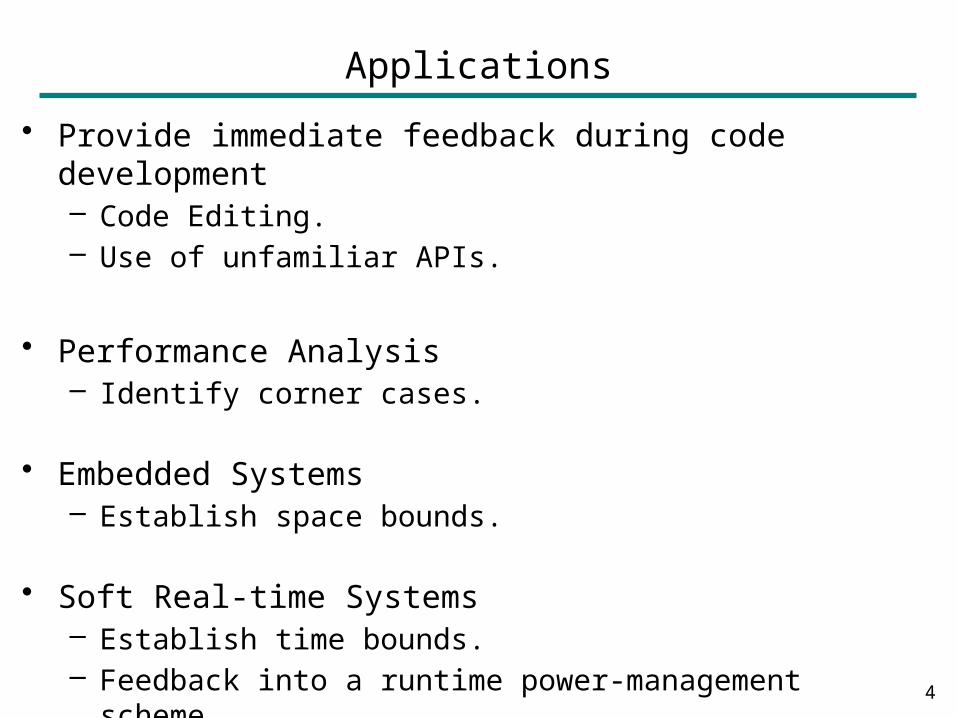
Applications

• Provide immediate feedback during code development– Code Editing.– Use of unfamiliar APIs.

• Performance Analysis– Identify corner cases.

• Embedded Systems– Establish space bounds.

• Soft Real-time Systems– Establish time bounds.– Feedback into a runtime power-management scheme.

4

Outline

Challenges in Bounds Analysis

• Idea #1: Proof Structure (control flow)

• Idea #2: Quantitative Functions (data-structures)

5

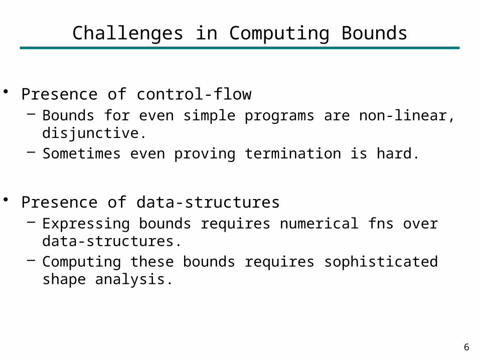
Challenges in Computing Bounds

• Presence of control-flow– Bounds for even simple programs are non-linear,

disjunctive. – Sometimes even proving termination is hard.

• Presence of data-structures– Expressing bounds requires numerical fns over data-

structures.– Computing these bounds requires sophisticated shape

analysis.

6

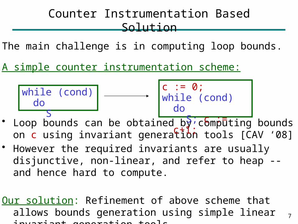
Counter Instrumentation Based Solution

The main challenge is in computing loop bounds.

A simple counter instrumentation scheme:

• Loop bounds can be obtained by computing bounds on c using invariant generation tools [CAV ‘08]

• However the required invariants are usually disjunctive, non-linear, and refer to heap -- and hence hard to compute.

Our solution: Refinement of above scheme that allows bounds generation using simple linear invariant generation tools.

7

while (cond) do

S

c := 0;while (cond) do S; c := c+1;

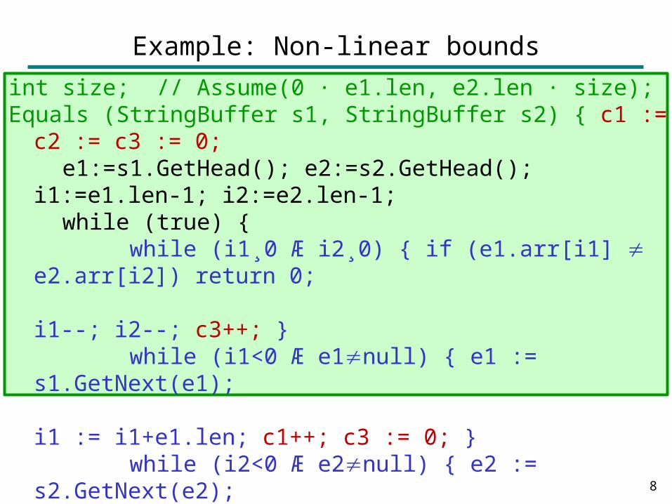
int size; // Assume(0 · e1.len, e2.len · size);Equals (StringBuffer s1, StringBuffer s2) { c1 := c2 :=

c3 := 0; e1:=s1.GetHead(); e2:=s2.GetHead(); i1:=e1.len-1;

i2:=e2.len-1; while (true) { while (i1¸0 Æ i2¸0) { if (e1.arr[i1] e2.arr[i2]) return

0; i1--; i2--; c3++; } while (i1<0 Æ e1null) { e1 := s1.GetNext(e1); i1 := i1+e1.len; c1++; c3 :=

0; } while (i2<0 Æ e2null) { e2 := s2.GetNext(e2); i2 := i2+e2.len; c2++; c3 :=

0; } if (i1<0) return (i2<0); if (i2<0) return 0; c3++; }; return 1; }• Total iterations of 2nd & 3rd inner loops: Len(s1) & Len(s2).• For each iteration of 2nd & 3rd inner loops, combined

iterations of 1st inner loop & outer loop: size• Therefore total complexity is

(1+size)*(1+Len(s1)+Len(s2))

Example: Non-linear bounds

8

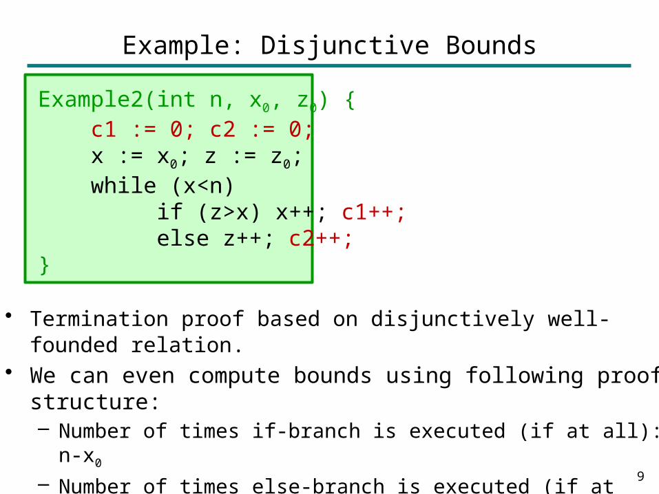
Example: Disjunctive Bounds

Example2(int n, x0, z0) { c1 := 0; c2 := 0; x := x0; z := z0; while (x<n) if (z>x) x++; c1++; else z++; c2++;}

• Termination proof based on disjunctively well-founded relation.

• We can even compute bounds using following proof structure: – Number of times if-branch is executed (if at all): n-x0

– Number of times else-branch is executed (if at all): n-z0

– Therefore, total iterations: Max(0,n-x0) + Max(0,n-z0)9

Outline

• Challenges in Bounds Analysis

Idea #1: Proof Structure (control flow)

• Idea #2: Quantitative Functions (data-structures)

10

Proof Structure

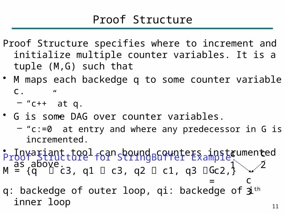
Proof Structure specifies where to increment and initialize multiple counter variables. It is a tuple (M,G) such that

• M maps each backedge q to some counter variable c.– “c++” at q.

• G is some DAG over counter variables.– “c:=0” at entry and where any predecessor in G is

incremented. • Invariant tool can bound counters instrumented as

above.

11

c1 c2

c3

Proof Structure for StringBuffer Example:M = {q c3, q1 c3, q2 c1, q3 c2,}

q: backedge of outer loop, qi: backedge of ith inner loop

G =

Computing bound from a proof structure

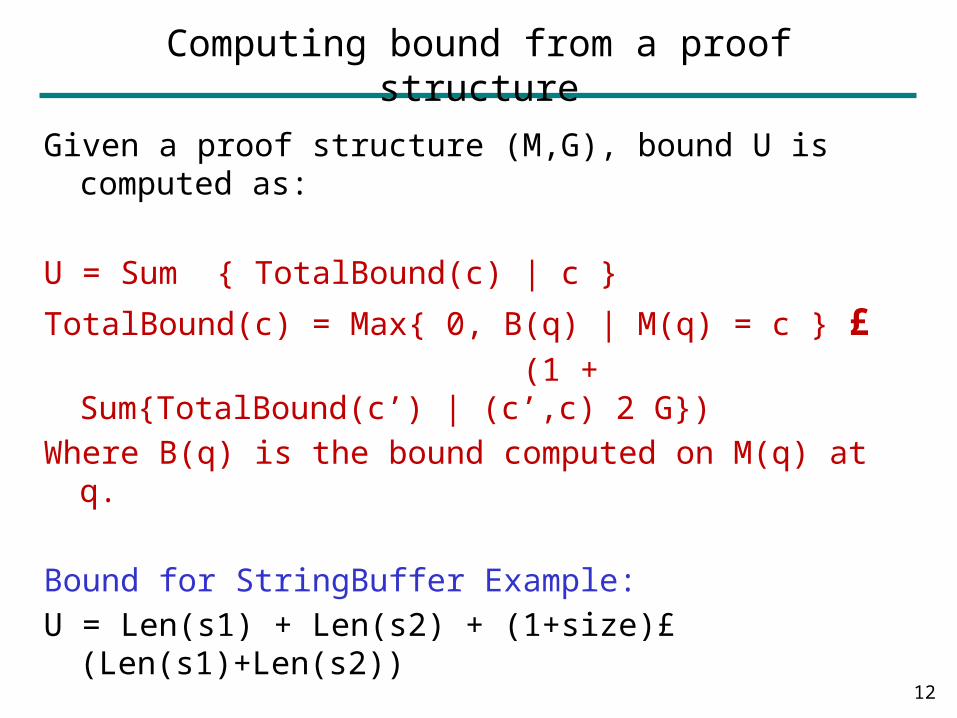
Given a proof structure (M,G), bound U is computed as:

U = Sum { TotalBound(c) | c }

TotalBound(c) = Max{ 0, B(q) | M(q) = c } £ (1 + Sum{TotalBound(c’) | (c’,c) 2

G})Where B(q) is the bound computed on M(q) at q.

Bound for StringBuffer Example:U = Len(s1) + Len(s2) + (1+size)£

(Len(s1)+Len(s2))

12

Automatically Computing Proof Structure

• Total number of potential proof structures (M,G) are exponential in number of back-edges.– Hence a naïve search is expensive.

• Key Idea: Increasing counters and dependencies increases ability of an invariant generation tool to discover bounds.– But cannot simply make all counters depend on each

other.– Need to find right set of dependencies that create a DAG.

• There is a quadratic (in number of back-edges) algorithm to compute a (counter-optimal) proof structure. [POPL ’09]– A counter-optimal proof structure uses minimal counters

and miminal dependencies between counters.– Generally, this leads to more precise bounds.

13

Outline

• Challenges in Bounds Analysis

• Idea #1: Proof Structure (control flow)

Idea #2: Quantitative Functions (data-structures)

14

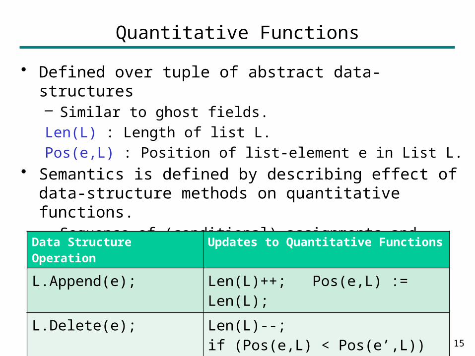
Quantitative Functions

• Defined over tuple of abstract data-structures– Similar to ghost fields.Len(L) : Length of list L.Pos(e,L) : Position of list-element e in List L.

• Semantics is defined by describing effect of data-structure methods on quantitative functions.– Sequence of (conditional) assignments and assumes.– Can also refer to unscoped variables (universally

quantified).

15

Data Structure Operation

Updates to Quantitative Functions

L.Append(e); Len(L)++; Pos(e,L) := Len(L);

L.Delete(e); Len(L)--; if (Pos(e,L) < Pos(e’,L)) Pos(e’,L) --;

e1 := L.GetNext(e2); Pos(e1,L) := Pos(e2,L)+1;Assume(Pos(e1,L) · Len(L));

Principles behind defining Quantitative Functions

• Precision– Defining more quantitative fns. increases ability of linear

invariant generation tool to find bounds.– In practice, a few quantitative fns are usually sufficient.

• Soundness– Method annotations are always sound from tool’s

perspective.– User’s responsibility to ensure that intended semantics

matches with the method annotations.– Verification is possible if intended semantics can be

described in an appropriate logic• Gulwani, Sagiv, Lev-Ami: “A Combination Framework for

Tracking Partition Sizes”, POPL 2009.

16

Computing Invariants over Quantitative Functions

• Instrument a data-structure method call with its effect allowing quantitative fns. to be treated as uninterpreted.– Instantiate unscoped variables with all appropriate

terms.• Use a linear invariant generation tool with support for

uninterpreted functions.– Abstract Interpretation based Technique.

Combine Polyhedron abstract domain [Cousot, POPL ‘79]

with uninterpreted fns domain [Gulwani, Necula, SAS’ 04]

using domain-combinators [Gulwani, Tiwari, PLDI ‘06]– Constraint-based Invariant Generation Technique. [Beyer et.al., VMCAI ‘07]

17

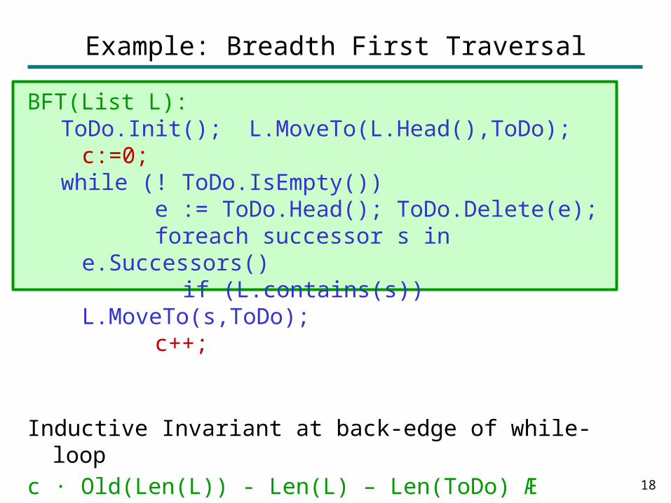
Example: Breadth First Traversal

BFT(List L): ToDo.Init(); L.MoveTo(L.Head(),ToDo); c:=0;while (! ToDo.IsEmpty()) e := ToDo.Head(); ToDo.Delete(e); foreach successor s in e.Successors()

if (L.contains(s)) L.MoveTo(s,ToDo); c++;

Inductive Invariant at back-edge of while-loopc · Old(Len(L)) - Len(L) – Len(ToDo) Æ Len(L) ¸ 0 Æ Len(ToDo) ¸ 0

This implies a bound of Old(Len(L)) for while loop.18

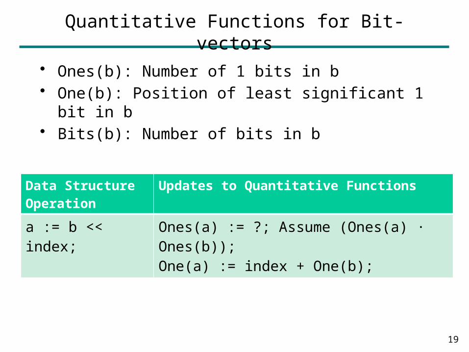
Quantitative Functions for Bit-vectors

• Ones(b): Number of 1 bits in b• One(b): Position of least significant 1 bit in b• Bits(b): Number of bits in b

19

Data Structure Operation

Updates to Quantitative Functions

a := b << index; Ones(a) := ?; Assume (Ones(a) · Ones(b));One(a) := index + One(b);

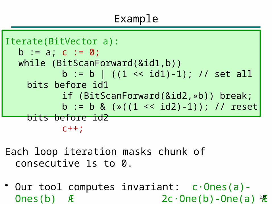
Example

Iterate(BitVector a): b := a; c := 0;while (BitScanForward(&id1,b)) b := b | ((1 << id1)-1); // set all bits before id1 if (BitScanForward(&id2,»b)) break; b := b & (»((1 << id2)-1)); // reset bits before id2 c++;

Each loop iteration masks chunk of consecutive 1s to 0.

• Our tool computes invariant: c·Ones(a)-Ones(b) Æ 2c·One(b)-One(a) Æ One(b)·Bits(a)

• This implies bound of Min {Ones(a), Bits(a)/2 } 20

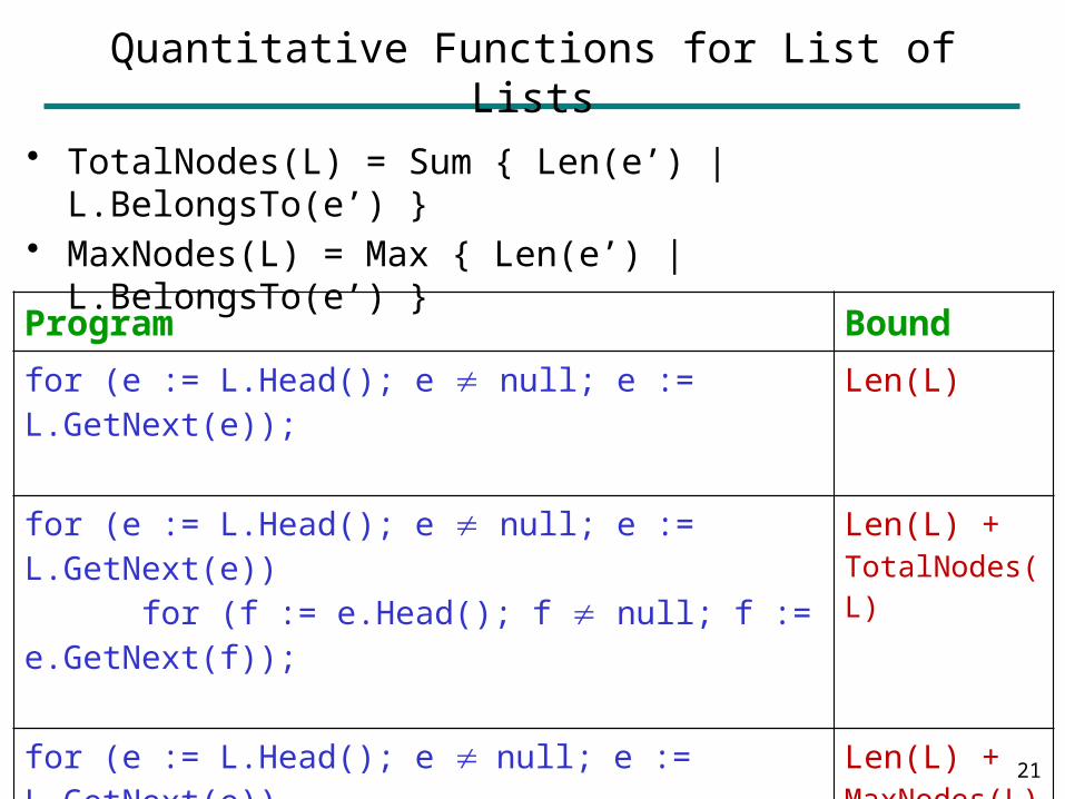
Quantitative Functions for List of Lists

• TotalNodes(L) = Sum { Len(e’) | L.BelongsTo(e’) }• MaxNodes(L) = Max { Len(e’) | L.BelongsTo(e’) }

21

Program Boundfor (e := L.Head(); e null; e := L.GetNext(e)); Len(L)

for (e := L.Head(); e null; e := L.GetNext(e)) for (f := e.Head(); f null; f := e.GetNext(f));

Len(L) + TotalNodes(L)

for (e := L.Head(); e null; e := L.GetNext(e)) if (*) break;for (f := e.Head(); f null; f := e.GetNext(f));

Len(L) + MaxNodes(L)

Quantitative Functions for Trees

Nodes(T): Total number of nodes in tree THeight(T): Height of tree T

22

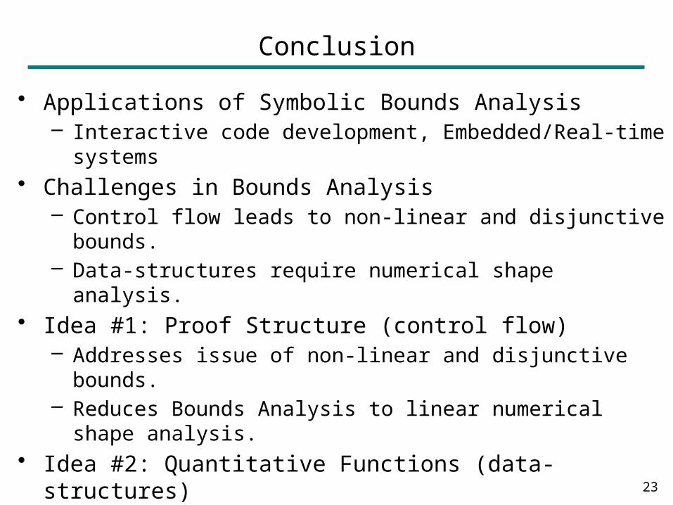
Conclusion

• Applications of Symbolic Bounds Analysis– Interactive code development, Embedded/Real-time

systems• Challenges in Bounds Analysis

– Control flow leads to non-linear and disjunctive bounds.– Data-structures require numerical shape analysis.

• Idea #1: Proof Structure (control flow)– Addresses issue of non-linear and disjunctive bounds.– Reduces Bounds Analysis to linear numerical shape

analysis. • Idea #2: Quantitative Functions (data-structures)

– Further reduces Bounds Analysis to linear invariant generation over uninterpreted functions.

23