Speculative Plan Execution for Information Gathering · 1 Speculative Plan Execution for...

1

Speculative Plan Execution for Information Gathering

Greg Barish [email protected] Fetch Technologies 2041 Rosecrans Avenue, Suite 245 El Segundo, CA 90245 USA Craig A. Knoblock [email protected] University of Southern California Information Sciences Institute 4676 Admiralty Way Marina del Rey, CA 90292 USA

Abstract

The execution performance of an information gathering plan can suffer significantly due to remote I/O latencies. A streaming dataflow model of execution addresses the problem to some extent, exploiting all natural opportunities for parallel execution, as allowed by the data dependencies in a plan. Unfortunately, plans that integrate information from multiple sources often use the results of one operation as the basis for forming queries to a subsequent operation. Such cases require sequential execution, an inefficiency that can erase prior gains made through techniques like streaming dataflow. To address this problem, we present a technique called speculative plan execution, an out-of-order method that capitalizes on knowledge gained from prior executions as a means for overcoming remaining data dependencies between plan operators. Our approach inserts additional plan operators that generate and confirm speculative results, while preserving the safety and fairness of overall execution. To increase the utility of speculative execution, we propose a method of value prediction that combines caching with the more effective and space-efficient techniques of classification and transduction. We present experimental results that demonstrate how the performance of information gathering plans can benefit from speculative execution and how its overall utility can be increased through our hybrid method of value prediction. Keywords: plan execution, speedup learning, information agents

1. Introduction The ubiquity of computer networking has created the potential for many types of data to be combined and processed in all sorts of useful ways. Nowhere is the benefit of such networking more obvious than it is on the Internet. Millions of people use the Web every day to research airfares, monitor financial portfolios, and keep up to date with the latest news headlines. The capability of integrating data from multiple sources on networks like the Internet allows users to accomplish a limitless number of useful tasks.

Unfortunately, manually gathering data from a collection of remote sources, like Web sites, can be tedious and time consuming. To accomplish a given task, one must often query multiple sources in a certain order. Worse, it is often necessary to navigate through sets of intermediate data en route to the exact information being sought. Also, throughout the process, one is often required to keep track of data gathered earlier, in order to combine it with data gathered later.

For example, consider the task of using multiple Web sites for purposes of researching a car to buy. Suppose that, when choosing a car based on some criteria (say year and type), we are interested not only in the price, but also in reviews of the car, as well as recent safety ratings. To

2

gather this information manually may require that we use one Web site to identify which cars are in our price range. Then, for each car that does meet our price constraints, we need to browse to all of the reviews, possibly at a different site. Finally, again for each candidate car, we may need to visit a yet another site to obtain recent car safety ratings. Although the Web contains all of this information, it is a time consuming process to manually search and click through to all of the data. Some variations of this type of search (e.g., searching for a house) are even worse to consider because the frequency of executing this task is higher, with the same steps are repeated over and over again.

Information mediators (Wiederhold, 1996; Bayardo et al., 1997; Knoblock et al., 2001) and software agent execution systems (Eztioni and Weld, 1994; Lesser et al., 2000; Sycara et al., 2003; Barish and Knoblock, 2005) enable these types of tedious information gathering tasks to be automated. For example, a relatively simple agent can be constructed to gather all of the information about the cars that match a specified search criteria, including reviews and safety ratings. Such agents can also become useful Web applications – Froogle, Shopzilla, and PriceGrabber are just a few examples of widely-used Web applications that function as information agents. Such applications integrate data from other Web or database-style sources, presenting the result of integration in a single user interface for the end-user.

1.1 The performance problem While information agents automate what is normally a tedious manual task, such agents can be slow to execute, especially if the data must be gathered from a source that is not local. For example, when querying a remote Web site, latencies can vary tremendously, from a few hundred milliseconds to several seconds. Not only does the agent pay a small penalty to access the information remotely, but the rate at which the remote source can answer a query often depends on its load at the time the query was submitted.

The inefficiency of information gathering plans has become a topic of research for both network query engines (Ives et al., 2002; Naughton et al., 2001; Hellerstein et al., 2003) and information agents (Barish and Knoblock, 2005). Since it is impossible to control the performance of the network or of the remote sources, research has instead focused on strategies for increasing the degree of run-time parallelism. Towards that end, various parallel execution techniques such as dataflow-style plan representation, data pipelining, remote query optimization, and adaptive query execution have been emerged. The latter category includes techniques such as adaptive tuple routing (Avnur and Hellerstein, 2000), double pipelined hash joins (Ives et al., 1999), and approximate query results (Shanmugasundaram et al., 2000).

Despite the benefits of all of these techniques, data dependencies between operators can still significantly hamper execution. For example, a query to a remote source can depend on the answer of a query to a previous source. In the car search scenario, for instance, the agent cannot gather safety ratings for cars until an earlier query that identifies candidate cars based on price and basic features completes. If the query to find the list of candidate cars takes 2 seconds to be answered and the safety ratings query takes 2 seconds, then the overall plan will take 4 seconds to execute. None of the currently proposed execution optimizations can improve upon this, because of the remote data dependency involved. Such binding-pattern style relationships require sequential execution and thus offer no opportunity for parallelization.

Four seconds may not seem like a long time, especially considering the benefit of the automation, but for agents that are deployed as Internet applications, such performance can be an eternity. Every increase in basic plan execution time decreases the throughput of how many queries can be processed per unit time. Per Little’s Law (Little, 1961), assuming that a service

3

has a fixed amount of a set of resources and that the arrival rate is constant, longer plan execution times will lead to longer queues and thus longer wait times. In short, a minor wait can translate into a major throughput problem for popular agents.

1.2 Speculative execution: a new type of run-time parallelism To combat persistent latencies, and to capitalize on the knowledge gained from prior executions, we present an approach for the speculative execution of information gathering plans. In computer architecture, speculative execution is the process of executing instructions ahead of their normal schedule. Nearly all modern CPUs employ this technique as a means to address the I/O latencies associated with accessing local RAM. The underlying idea is that it is more efficient to probabilistically use an otherwise idle CPU than to not use it at all. As long as the benefits of successful speculative execution outweigh the total overhead of its use, the technique is considered a profitable activity. Research has shown that speculative execution remains one of the most effective means for increasing the level of instruction level parallelism (ILP) during program execution (Wall, 1990).

Just as speculation improves ILP for programs, we show how it can also be used to increase the degree of operator-level parallelism during the execution of information gathering plans. By speculating about the execution of future operators, it is possible to overcome CPU delays caused by earlier I/O-bound operators (e.g., those fetching remote data) and deliver better performance. Thus, speculative execution directly addresses the problem of data dependent operators executing in environments with available resources. Further, applying speculative execution at a level higher than that of machine instructions enables two additional benefits:

• Significant performance improvement. Since information gathering latencies can be quite high, speculative execution of plan operators allows gains to often be made in terms of seconds, with resulting speedups exceeding a factor of two.

• The opportunity to apply more intelligent techniques to the problem of speculation. CPU-level speculative execution must rely on limited resources – and thus limited techniques – when predicting program control and data flow. In contrast, plan-level speculative execution can leverage more resources and reap the benefits that more sophisticated techniques can offer.

1.3 Contributions of this paper In this paper, we describe an approach to speculative plan execution and demonstrate how it can improve the performance of information gathering. We also present an approach to value prediction that combines classification and transduction in order to generate predictions from hints in an intelligent, space-efficient manner. Specifically, the contributions of this paper are:

• An approach for speculative plan execution that yields arbitrary speedups, while ensuring safety and fairness.

• Algorithms for automatically transforming any information gathering plan into one capable of speculative execution.

• Algorithms for learning string transducers that combine caching, classification, and substring transduction in order to generate predictions from hints.

The rest of this paper is organized as follows. The next section reviews how information gathering plans are executed. In Section 3, we describe our approach to speculative execution in detail. Section 4 describes how machine learning can be applied to improve value production,

4

specifically how classification and transduction can be used to build efficient and intelligent value predictors. Section 5 details the related work and Section 6 concludes our discussion.

2. Executing information gathering plans We start by reviewing the details of how information gathering plans are executed. Generally speaking, an information gathering plan is any type of plan that collects, processes, and integrates information from one or more sources. The plan is formed by a higher level query processing system, such as an information mediator. For example, the Prometheus and Ariadne mediators (Thakkar et al. 2005; Knoblock et al. 2001), reason about sources and form information gathering plans to be executed, just as a compiler forms a series of machine instructions to execute. Once formed, such plans can be executed by systems such as Theseus [Barish & Knoblock, 2005]. While an executor may use many techniques to efficiently process the plan, such as streaming or novel tuple routing techniques, it does not typically re-engage in higher-level planning, such as reasoning about sources.

Execution plans consist of a partially-ordered graph of operators Op1..Opn connected in a producer/consumer fashion. Each operator consumes a set of inputs a1..ap, fetches data or performs a computation based on that input, and produces one or more outputs b1..bq. The types of operators used in information gathering plans vary, but most either retrieve or perform computations on data.

Data may be retrieved from a variety of sources, including databases, Web services, and Web sites. The latter is more involved – one must first fetch a Web page from a remote source and then extract from that page, typically based on some extraction rules that have been hand-coded or automatically generated. Operators that perform this task are called wrappers. These operators can often be slow to execute because a remote Web site may be busy and also because the data being requested (the HTML) may be large (though the amount of data extracted may be small). Unfortunately, the remote Web site is typically not under the administrative control of the person that wishes to extract data from it, so he or she may encounter unpredictable delays. In this paper, we will frequently refer to example plans that gather data via Wrapper operators, although any operator that gathers data from a network source can exhibit the same fundamental problem: dependency on a remote entity with varying response latencies.

2.1 Streaming dataflow plan execution There are two basic types of parallelism that are frequently exploited when executing information gathering plans. One is horizontal parallelism, or operator parallelism, which is the notion of multiple operators executing concurrently. A second is vertical parallelism, or data parallelism, which is where a larger unit of data can be broken up into smaller units so that the larger unit is effectively processed in parallel by multiple operators.

Horizontal parallelism is realized through dataflow-style execution of information gathering plans, where the plan is represented as a partially ordered graph. Operators act as nodes in the graph, while the input and output variables for each operator determine the edges. During execution, producer operators transmit data to consumer operators in terms of relations, where each relation R consists of a set of attributes (i.e., columns) a1..ac and a set of zero or more tuples (i.e., rows) t1..tr, each tuple ti containing values vi1..vic. We can express relations with attributes and a set of tuples as: R (a1..ac) = {{v11..v1c}, {v21..v2c}, ... {vr1..vrc}} . Note that relations are not necessarily the only type of data that can be communicated between operators; however, in practice it is very common, particularly since many years of database research has focused on processing relational data.

5

Vertical parallelism is exploited by streaming data between producer and consumer operators. This is accomplished by transmitting data at the tuple level. In doing so, there needs to be a way to signal that the stream has completed transmission. This is the function of a special end-of-stream (EOS) token, transmitted from a producer to a consumer after the last tuple has been sent. As a result of streaming, the firing rule of an operator changes from “whenever a relation arrives” to “whenever a tuple arrives.” Streaming is a powerful feature for information gathering plans, as it allows data to be processed as it trickles out from a remote source. At the same time, it is more complex to implement because it requires operators to maintain state in between firings.

Combining both types of parallel execution is commonly referred to a streaming dataflow and is a technique that has been applied to network queries (Naughton et al., 2001, Hellerstein et al., 2000, Ives et al., 2002) and information agents (Barish and Knoblock, 2005). Streaming dataflow represents the maximum amount of “natural” parallelism possible by exploiting, where possible, the independence of operations and/or data.

2.2 Example execution To better understand the benefits of streaming dataflow, and to set the stage for our later discussion of speculative execution, let us consider the details of an example Web information agent plan. In doing so, we return to the earlier example of an agent that assists the user who is interested in buying a new car.

CarInfo is an agent that collects reviews and safety ratings of used cars that meet a specific set of user search criteria. The criteria are composed of car type, year of original production, and a desired price range. The user also specifies a list of car makers to avoid. Once it receives its input data, CarInfo uses a collection of Web sources to gather the appropriate results. In particular, three different Web sources are used:

• Edmunds.com, to get a list of used car models meeting the initial search criteria. • ConsumerGuide.com, to obtain the reviews for those models. • NHTSA.gov (National Highway Traffic Safety Association), for crash safety ratings of

those models.

The Web pages for each of these sources is shown in Figures 2.1a-c.

Figure 2.1a: Edmunds car search results page

Figure 2.1b: NHTSA safety ratings page

6

CarInfo first gathers the list of cars from Edmunds, filters out those automakers that the user would like to avoid (Edmunds does not allow this to specified through its search interface), gathers the safety reports from NHTSA for the filtered set of cars, combines this result with reviews gathered at ConsumerGuide and then outputs the results. A dataflow-style plan for CarInfo that performs these operations is shown in Figure 2.2.

As the figure shows, the independence of the NHTSA and ConsumerGuide queries allows both to execute concurrently. Also note the complexity of gathering the car reviews from ConsumerGuide, specifically that additional navigation is required. CarInfo must first query ConsumerGuide through its search interface to find a pointer to the summary page for that car. It then queries the summary page to find the detailed review page. Finally, it gathers the review text from the detailed review page. Engaging in additional navigation in order to extract the desired information is a common subtask for Web agents in particular, since Web sites are designed to be visually browsed and may not support the direct querying of all the information they provide.

As a detailed example of CarInfo execution, consider the case where the initial search criteria is (Midsize sedan, year 2002 model, minimum price $4000, maximum price $12000) and the cars to avoid are those by the auto maker (Oldsmobile). During execution, the first Wrapper operator returns (Oldsmobile Alero, Dodge Stratus, Pontiac Grand Am, Mercury Cougar). From these, filtering out of Oldsmobile models results in the subset (Dodge Stratus, Pontiac Grand Am, Mercury Cougar). The safety reports and full reviews of these cars are then queried. For

Figure 2.1c: ConsumerGuide car reviews page

Figure 2.2 Dataflow-style version of CarInfo information agent plan

WRAPPERConsumerGuide

Search

search criteria


Summary


Full Review

WRAPPEREdmundsSearch

JOIN

SELECTmaker !=

"Oldsmobile"

WRAPPERNHTSASearch

result

7

example, for the first tuple (Dodge Stratus), the URL for the summary review of that car is (http://cg.com/summ/20812.htm) and the URL for the full review is (http://cg.com/full/20812.htm). Once at the full review URL, the review text can be extracted and joined with the safety report.

The CarInfo plan is one common type of information agent plan. Similar plans that extract data from two or more distinct sources and then combine them together are common throughout the literature (Friedman et al. 1999; Ives et al. 1999; Barish et al. 2000; Barish and Knoblock 2002). Like CarInfo, these plans also involve extracting and combining data from multiple sources using relational-style operations. Furthermore, note that the particular CarInfo plan generated for execution is not important; it is just an example of one type of plan. The actual plan generated will vary per the query processing system (mediator, etc.) that produces it.

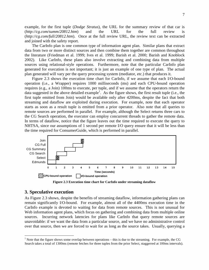
Figure 2.3 shows the execution time chart for CarInfo, if we assume that each I/O-bound operation (i.e., a Wrapper) requires 1000 milliseconds (ms) and each CPU-bound operation requires (e.g., a Join) 100ms to execute, per tuple, and if we assume that the operators return the data suggested in the above detailed example1. As the figure shows, the first result tuple (i.e., the first tuple emitted from Join) would be available only after 4200ms, despite the fact that both streaming and dataflow are exploited during execution. For example, note that each operator starts as soon as a result tuple is emitted from a prior operator. Also note that all queries to remote sources are performed in parallel. For example, although the Select returns three cars to the CG Search operation, the executor can employ concurrent threads to gather the remote data. In terms of dataflow, notice that the figure leaves out the time required to execute the query to NHTSA, since our assumptions of 1 second per remote I/O query ensure that it will be less than the time required for ConsumerGuide, which is performed in parallel.

3. Speculative execution As Figure 2.3 shows, despite the benefits of streaming dataflow, information gathering plans can remain significantly I/O-bound. For example, almost all of the 4400ms execution time in the CarInfo example is devoted to waiting for data from remote sources. This is not unusual for Web information agent plans, which focus on gathering and combining data from multiple online sources. Incurring network latencies for plans like CarInfo that query remote sources are unavoidable: if we want the data from a particular source, and we have no administrative control over that source, then we are forced to wait for as long as the source takes. Usually, querying a

1 Note that the figure shows some overlap between operations – this is due to the streaming. For example, the CG Search takes a total of 1300ms (remote fetches for three tuples from the prior Select, staggerred at 100ms intervals).

Figure 2.3 Execution time chart for CarInfo under streaming dataflow

Time (seconds)

0 1 2 3 4 5 6 7 8 9 10 11 12 13 14 15

SelectEdmunds

CG SearchCG Summary

CG FullJoin

CPU-bound operation I/O-bound operation

8

single source does not cause a noticeable degree of latency during execution. However, querying multiple data-dependent sources in sequence can often lead to a noticeable aggregate latency.

Unfortunately, the nature of information integration is such that there are often data dependencies, or binding patterns, between sources: that is, plans often need to gather data from one source and then use it to query another. Furthermore, information networks like the Web are designed to be browsed interactively by the user, requiring additional navigation in order to obtain a final answer (such as the details of a house or the full review of a car). Additional navigation typically involves chasing “Next Page” or “Details” links from a previous page, translating into even more data-dependent remote fetches. Such dependencies require the plan to be more sequential, leading to slower execution.

One of the primary remaining challenges associated with increasing the performance of Web query plans has to do with improving the extent to which flows that contain these types of binding-pattern relationships can be parallelized. For example, in the CarInfo plan, it is not normally possible to query NHTSA safety ratings and ConsumerGuide car reviews until Edmunds returns the list of cars that meet the initial search criteria. If we could somehow parallelize the gathering of ratings and reviews with the Edmunds search, the overall execution time would be dramatically improved. Unfortunately, this does not make logical sense: we cannot gather safety ratings and car reviews until we know which cars for which we need ratings and reviews. In short, the data dependencies between operators in a plan determine its performance barrier. This is better known as the dataflow limit.

3.1 The mechanics of speculative execution To overcome the natural dataflow limit of a plan, we introduce a new form of run-time parallelism: speculative plan execution. The intuition behind this technique is the use of hints received at earlier points in execution to generate speculative input data to dependent operators that occur later in a plan and execute them ahead of schedule. Through this method, consumer operators that are dependent on slow producers can be executed in parallel with those producers, using the input to those producers as hints about how to execute.

In speculative plan execution, the knowledge of how hints are associated with predictions is learned over time from earlier executions. As more knowledge is gained, accuracy (both precision and recall) can improve. And as accuracy improves, so does the average execution time of plans that employ speculative execution.

To better illustrate the how speculative execution can improve plan execution performance, let us return to the CarInfo plan example presented earlier. Consider the retrievals of the car reviews from ConsumerGuide and the safety ratings from NHTSA. Both activities occur in parallel, but both are dependent on the cars returned from Edmunds based on the user search criteria. As observed earlier, if Edmunds is slow, performance of the rest of the plan suffers.

With speculative execution, however, the input to Edmunds (the price range, the year, the type of car, mileage specifications, etc.) can be used to predict the inputs for the ConsumerGuide and NHTSA wrappers. For example, it could be learned that certain features of the search criteria (such as car type, year, and price range) are good predictors of the car makes and models that Edmunds will return. This would provide a reasonable basis upon which to predict queries to ConsumerGuide and NHTSA – even for input never previously seen. For example, once the system has seen the cars that the search criteria of (Midsize coupe/hatchback, 2002, $4000, $12000) returns, it is possible to make reasonable predictions about the cars that the criteria (Midsize coupe/hatchback, 2002, $5000, $11000) will return.

9

In this example, there is no reason why the system cannot speculatively execute retrievals for multiple sets of cars to improve the chances for success. For example, from prior executions, the system could learn that a price range of $4000-$12000 returns a result set RS1 and a price range of $8000-$16000 returns a result set RS2. When given a new criteria of $6000-$14000, the system could predict both RS1 and RS2. Identifying the correct subset occurs during the processing of the search at Edmunds. However, the capability to issue multiple sets of predictions at once allows us to have the best of both worlds – hedging both predictions – and confirming only those speculations that turn out to be correct. Speculatively executing the same path with multiple data can thus often be useful when hints map to multiple answers.

Speculative plan execution can enable the fetching of data from Edmunds, NHTSA, and ConsumerGuide to be run in parallel. Since all three tasks are almost entirely I/O-bound, using separate threads for each can result in almost true concurrent execution. It is important to realize, however, that we cannot speculate without caution. In particular, we need to be careful about how the output from the final Join operator is handled – that is, data should not exit the plan until the earlier predictions that led to it have been verified as correct.

In summary, this discussion of speculatively executing information agent plans has raised three important requirements. Specifically, for any approach, it is important to:

• Define a process for speculation and confirmation: It is important to specify how speculative execution works – what triggers it, how predictions are made, etc.

• Ensure safety: Speculative execution must be prevented from triggering an unrecoverable action (such as the generation of output or the execution of an operator affecting the external world) until earlier predictions has been verified. Thus, all speculation must be confirmed.

• Ensure fairness: Speculative execution should not be prioritized at the same level as normal execution. Its resource demands should be secondary. For example, the CPU should not be processing speculative instructions while normal instructions await execution.

In the remainder of this section, we describe how we address each of these three requirements, as well as where to predict and how to automatically transform plans for speculative execution. The problem of what to predict, which directly affects the utility of speculative execution, is addressed in detail in Section 4.

3.1.1 Speculation and confirmation The process we introduce for enabling speculative plan execution involves augmenting a standard information agent plan with two additional operators. The first, Speculate, is a mechanism for using hints to predict inputs to future operators, and later for correcting or confirming those predictions. The second operator, Confirm, halts the flow of speculative data beyond “safe points” in a plan until earlier predictions can be confirmed or corrected.

Figure 3.1 shows how these operators are deployed in a transformation of CarInfo for speculative execution. As the figure shows, a Speculate operator receives its hint (the search criteria) and uses it to generate predictions about car models. These cars, in turn, drive the remainder of execution, while the first part of execution continues. Note that the final Join can also be executed – the only requirement is that a Confirm operator exist somewhere after the Speculate operator and before the end of the plan. This prevents speculative results from exiting the plan until Speculate has confirmed its predictions.

10

J

SW

W

Speculate

Confirm

hintspredictions/additions

confirmationsanswers

WW

W

fa

fa

fb / fc fb

fc

The inputs and outputs of the Speculate operator are summarized in Figure 3.2. As the figure shows, this operator receives hints (input data to an earlier operator in the plan) and uses those hints to generate data predictions (used as input to operators later in the plan). These predictions are tagged as speculative; any further results they lead to are also tagged. Later, Speculate receives answers to its earlier predictions from the operator normally producing this data. Using these answers, confirmations can be generated to validate prior predictions. Any data errantly predicted is not confirmed and data that was never predicted is eventually forwarded via the predictions/additions output, without being tagged.

For example, in Figure 3.1, the search criteria are used to predict cars. Let us suppose these predictions are {X, Y}. This triggers the gathering and combining of safety ratings and car reviews, with the combination (joining) of this data held up at the Confirm operator. At the same time, suppose that the Speculate operator receives an answer that indicates that the real cars were { X, Z}. It can subsequently route confirmation for X to the Confirm operator. In contrast, Y is not confirmed because no such answer was received from Edmunds. In addition, Z is not tagged speculative and is propagated through to the ConsumerGuide, NHTSA, and Join operators. Note that Z does not require confirmation because it was never predicted (Confirm allows tuples not tagged for confirmation to pass through). As this example demonstrates, because Speculate operates at the tuple level, corrections to its predictions are fine-grained and require only the minimum amount of additional work be done to correct a mistaken prediction.

The behavior of the Confirm operator is to emit only confirmed results. Figure 3.3 illustrates its inputs and outputs: probable_results are the incoming speculative tuples, confirmations are generated by the Speculate operator, and actual_results are the filtered (correct) results. The role of Confirm is to guard against the release of unconfirmed or errant tuples beyond a safe point in the plan. The main way it differs from a relational Select operator is in how it uses the confirmations as a filter to halt probable_results tuples until each has been confirmed.

Confirmprobable_results

confirmationsactual_results

Figure 3.3: The Confirm operator

Figure 3.1: The CarInfo plan, modified for speculative execution

Speculateanswers

hints

confirmations

predictions/additions

Figure 3.2: The Speculate operator

11

Note that this approach exploits the fine-grained property of execution that data steaming provides. By basing production of verified results on confirmations – instead of errors – correct data can be output as soon as possible, without waiting for the remaining corrections to be processed. Confirm will continue to wait for corrections until it receives an EOS, which is controlled and propagated by the Speculate operator.

Finally, a note about the input to the Confirm operator. In Figure 3.3, it is shown as a single input. However, we assume that this input is actually a variable stream input. That is, it accepts multiple producers of the same data (each producer sending its own EOS) and unions together all of these streams. In this way, multiple producers of confirmations (i.e., multiple Speculate operators) can share the same Confirm operator. The advantage of this will become clear in later subsections.

3.1.2 Safety and fairness Ensuring safety during speculative execution means preventing errant predictions from affecting the external world in unrecoverable ways. As described above, the Confirm operator ensures safety by only producing verified results as long as it is correctly placed in a transformed plan. To maximize the benefits of speculative execution while ensuring correctness, Confirm is placed as far as possible along a speculative path, occurring just prior to plan output or an “unsafe operator”. This allows speculation to parallelize sequential flows as much as is safely possible. For example, in Figure 3.1, Confirm is located just prior to plan output.

Ensuring fairness means guaranteeing that normal execution is prioritized over speculative execution in terms of access to resources. For information gathering plans, the primary three resources to be concerned about are processing power (CPU), physical memory (RAM), and network bandwidth. Using existing technology, fairness with respect to the CPU can be ensured by the operating system. During execution, operators for information gathering systems are associated with threads and processing occurs at the tuple-level. By maintaining a pool of standard-priority “normal threads” and a pool of lower-priority “speculative threads”, the former can be used to handle the firing of operators under normal execution while the latter can be used for speculative execution. Standard operating system thread scheduling thus ensures that speculative CPU use never supersedes normal CPU use.

Memory can be metered by pooling objects. Operators can be written such that they draw memory from different pools, based on whether the objects being processed have been tagged as speculative. If so, new objects can be allocated from the speculative pool of those objects. The sizes of these pools can be adjusted as necessary, based on how much physical memory is allocated for speculative processing.

In terms of bandwidth, the goal is again to make sure that speculative use of bandwidth does not interfere with normal requests for bandwidth. Bandwidth reservation schemes such as RSVP (Zhang et al., 1993) are one way to provide such guarantees. In addition to hardware-based (e.g., network switch bandwidth provisioning) and software-based (e.g., TCP/IP socket configuration) methods, network resources can also be controlled by limiting the number of speculative threads and handles to network connection objects. This is similar to the solution for limiting memory use. A fixed number of threads and connection objects limits the number of simultaneous speculative use of resources and thus can assist in bounding the amount of speculative bandwidth (or any other resource) concurrently demanded.

3.1.3 The profitability of speculative execution The maximum, or optimistic performance, benefit resulting from speculative execution is equal to the minimum possible execution time of a transformed plan. Calculating this requires

12

computing the minimum execution times for each of the independent sequential flows of the plan and then choosing the maximum value of that set. Using the minimum execution time for each flow implies all predictions are correct and no further additions are needed.

For example, consider the optimistic performance of the plan in Figure 3.1. This plan shows three paths of concurrent execution (as labeled in the figure): the Edmunds flow fa, the NHTSA speculative flow fb, and the ConsumerGuide speculative flow fc. If we again assume that all network retrievals take 1000ms per tuple and all computations (Select, Join, Speculate, and Confirm) each take 100ms per tuple, the resulting flow performance for the first tuple is:

fa = 1000 + 100 + 100 = 1200 ms fb = 100 + 100 + 1000 + 100 + 100 = 1400 ms fc = 100 + 100 + 1000 + 1000 + 1000 + 100 + 100 = 3400 ms

Since the original time to first tuple (using these assumed values) would have been 4200ms, the potential speedup due to speculative execution in this case is 4200ms/3400ms = 1.24. Note that if Edmunds had been very slow, say 3200ms per tuple, overall original performance would have been slower (6400ms) and potential speedup (6400ms/3400ms = 1.88) greater.

3.2 Achieving better speedups While a speedup of about two allows execution time to be nearly halved, producing noticeable results, there is room for improvement. At first, it might not seem possible – since all speculation must be confirmed, execution time appears bound by either the time to perform speculative work or the time to process confirmation. For example, in Figure 3.1, we are either bound by the time required by initial and confirming flow fa or the speculative flows fb or fc.

However, two additional techniques can be used to increase the degree of speculative parallelism and the level of accuracy with respect to the prediction, both leading to significantly better speedups. The first involves using earlier speculation to drive later speculation, which increases the degree of speculative parallelism at runtime. The second is the concept of speculating multiple times per hint, which increases average recall for a particular speculative opportunity. We discuss both in detail, below.

3.2.1 Cascading speculation We are not limited to speculating about only one operator at a time. In fact, it is possible for speculation about one operator to trigger speculation about the next operator and so on, an effect we call cascading speculation. When the results of an initial prediction are known, this can trigger confirmation of the second prediction and so on, in effect cascading confirmations.

The performance benefit of cascading is the increase in speculative parallelism it allows, thus making it possible to achieve very high speedups. To illustrate, consider a longer sequence of operators, such as that in Figure 3.4. Recalling our earlier assumptions, processing ten wrapper operators in succession would normally require 10 seconds. Let us also assume that each operator consumes a single tuple of input and produces a single tuple of output. Predicting input f in Figure 3.4, which occurs midway in the sequence, allows the first and last halves of the

W

a

W W

b c

W

d

W W

e f

W

g

W W

h i

W

j

Figure 3.4: A longer sequence of operators

13

plan to execute concurrently, resulting in a new execution time of 5 seconds and a speedup of 2. With a single Speculate operator, this is the maximum speedup possible.

However, suppose that we wanted to use a to speculate about the input b to a second Wrapper, use the speculation of b to predict c, and so on. This is shown in Figure 3.5 (each Speculate operator is denoted by an S; Confirm by a C). Note that in the case of cascading speculation, one Confirm is still all that is required, as this operator is used to generally verify speculative tuples and requires no knowledge of when or why the speculation occurred2. It simply determines if each answer tuple is either a speculative output or a product of an earlier speculative output. If so, the tuple is held up until the confirmation(s) for that tuple have arrived.

Since all wrappers require the same amount of time to execute and are all I/O-bound, they would act simultaneously (the 1000ms remote source latency parallelized) and their confirmations could be processed at once. Thus, the resulting execution time would simply be the duration of a single wrapper call plus the overhead for speculation and the time to process confirmation. Even if we assume that the overhead and confirmation somehow requires an additional 100ms, execution would still only require 1000+100+100=1200ms, a speedup of 8.33.

Figure 3.6 shows a version of the speculative CarInfo plan in Figure 3.1 further modified for cascading speculation. Using earlier timing assumptions, then the five flows require the execution times shown in Table 3.1. Since execution time would be limited to the slowest of these flows, the optimistic speedup for the first tuple would be (4200ms/1600ms = ) 2.63.

2 Recall that the Confirm operator can take a variable number of confirmation inputs. For dataflow plan languages that do not support variable inputs, cascading speculation would still be possible by arranging a sequence of Confirm operators in place of the single Confirm operator shown in Fig 3.5.

W

J

W

W

SPEC

CONFIRM

SPEC

W

WSPEC

S

Figure 3.6: CarInfo modified for cascading speculation

W W W W W W W W W W

S S S S S S S S S

C

Figure 3.5: Cascading speculation of the sequence in Figure 3.4

14

Plan flow Execution time (ms)

Edmunds + Spec + Confirm 1200

Spec + Select + CG Search + Spec + Confirm 1400

Spec + Select + Spec + CG Summary + Spec + Confirm 1500

Spec + Select + Spec + Spec + CG Full + Join + Confirm 1600

Table 3.1: Optimistic execution times for CarInfo flows shown in Figure 3.6

Intuitively, cascaded speculation seems to make the most sense for navigational sequences, such as the three successive fetches from ConsumerGuide in the CarInfo plan. Many Web sources present a visual view of an underlying relational database schema. HTML pages are programmatically generated and thus navigation to certain data often tends to follow some simple URL patterns. Once prediction to the initial page is confirmed, all subsequent navigation is almost always verified because it predictably follows from the first page. Thus, for information gathering plans that speculate about interleaved navigation, cascading speculation can often overcome the cost of interleaved navigation.

This specific case occurs in the CarInfo plan. Consider the lower half of the plan in Figure 3.1, where ConsumerGuide is queried for car reviews. Once the dynamic part of the target URL is discovered (the car ID, “20812” in the case of the Dodge Stratus example earlier), the subsequent navigational pages are predictable. As a result, use of cascading speculation can easily yield a speedup of 3 for this interleaved navigation sequence.

3.2.2 Simultaneous speculation A second technique that can lead to better speedups for speculative plan execution is simultaneous speculation, the concept of making multiple sets of predictions. This technique acts as a “hedging” device for a Speculate operator; even if predictions about some tuples are incorrect, others may be correct and the additional number of predictions can improve recall.

Nevertheless, it is important to limit how many additional speculations are made on behalf of a single hint. Too many speculations can increase the overhead of speculative execution in several ways. First, each speculation leads to additional speculative work by one or more threads. For example, in the case of CarInfo, each extra prediction of what Edmunds might return requires work by at least 6 threads (one for each normal operator) + 3 additional threads (two additional Speculate and one Confirm operator), a total of 9 threads.

A second way that multiple speculations can increase overhead is by severely impacting a resource. For example, if one hundred different cars from Edmunds are predicted based a single hint (when in fact there are only 3 or 4 actual answers), the NHTSA and ConsumerGuide websites might be adversely affected by the additional load placed on their servers, which in turn affects the execution of the CarInfo plan.

However, for certain scenarios, multiple speculations are a reasonable and effective way to increase recall. For example, if a Speculate operator is predicting the result from a weather forecasting site, there may only be a few possible predictions (e.g., ”sun”, “clouds”, “rain”, “snow”, or “wind”). If the forecasting site is slow, it may be worthwhile to predict all five, knowing that only one will eventually be confirmed. By predicting all five, there is a guarantee that recall will be 100%, despite the fact that precision obviously worsened to 20%.

15

3.3 Automatic plan transformation In the previous section, we described how speculative plan execution can yield significant performance gains. However, in that example, augmentation of the CarInfo plan was done manually. In this section, we introduce algorithms that enable the automatic transformation of any information gathering plan into one capable of speculative execution.

The overall goal is to maximize the theoretical average performance gain resulting from speculative execution. At the same time, we also need to be wary of the overhead (cost) of speculative execution. Thus, we would like to identify the best speculative transformation P′i of a plan P, from some larger set of possible transformations P′1..P′m, that are different transformations of P for speculative execution.

3.3.1 The set of candidate transformations One natural way to approach the problem is to first generate the set of all possible speculative transformations and then iterate through this set, applying the equation above to identify the speculative transformation with the best theoretical execution time. Unfortunately, this approach is impractical because the set of all possible speculative transformations is huge.

To demonstrate why this is the case, let us consider how to calculate the number of possible speculative transformations for certain class of very simple information gathering plans that is a subset of the larger set of all possible plans. The class of plans considered is those that:

(i) are composed of a single, unbroken chain of n operators (ii) consist of operators that all have single input and single output (e.g., not Join)

(iii) have one plan input and one plan output

For example, the plan shown in Figure 3.7 meets these requirements.

To calculate the number of possible speculative transformations of a particular plan, it is

assumed that we are only interested in transformations where:

• all speculations involve using the input of an upstream operator as a hint for predicting the input of a downstream operator

• there can be one or more speculations in the plan (i.e., cascading speculation) • the same downstream input is not predicted by multiple upstream inputs

For example, there are five possible transformations for the plan shown in Figure 3.7, which can be summarized as:

((b|a), (c|a), (b|a, c|a), (c|b), (b|a, c|b))

This list denotes the set of possible transformations. Each transformation involves one or more instances of using a particular variable as a hint for issuing predictions about another variable. The list above simply describes the hint/prediction pairs for each transformation. The “|” means that the left-hand side variable could be predicted by the right-hand side variable (which always precedes the left-hand side in the plan). For example, the transformation (b|a,

A

a

B C

b c

Figure 3.7: Sample plan that meets (i), (ii), and (iii)

16

c|b) is one where “a” is used to predict “b” and “b” (speculative “b”, that is) is used to predict “c”. Thus, in this example, there are two Speculate operators and one Confirm.

To consider the total number of potential speculative transformations, we observe that for operator sequences of lengths 2, 3, and 4, the total possible number of transformations is 1, 5, and 23, respectively. Generally speaking, the number of transformations for a sequence of length n consists of the number of transformations required for a sequence of n-1 plus the number of transformations possible that involve the added operator. Specifically, the total number of possible speculative transformations ST(n) for a particular sequence of n operators for plans is roughly equal to the factorial series for n; even simple plans of moderate length can quickly generate a very large number of candidate transformations to evaluate3. For example, even under the fairly strict set of assumptions described earlier, a sequence of 10 operators has 3,628,799 possible speculative transformations.

3.3.2 Reducing the number of possible transformations The problem with using a brute force approach to identify the most profitable plan transformation is the factorial blowup of the number of candidate transformations. The problem obviously worsens for larger plans and even more dramatically when we relax earlier assumptions, such as that plans can only consist of a single flow. At the same time, intuition suggests that it is better to focus on how speculation might reduce the impact of major bottleneck operators in a plan, instead of considering every possible speculative opportunity.

We can reduce the size of the candidate transformation set substantially by leveraging Amdahl’s Law, which states that program execution time is a function of its most latent sequence of instructions. Thus, it is not worthwhile to consider transformations involving operators that do not exist in this sequence because any improvement cannot improve overall execution time.

Instead, Amdahl’s Law suggests that performance optimization should be focused on the costliest flow in the plan. In particular, we can use a most-expensive-path (MEP) approach that identifies the most latent sequence of operators in an information gathering plan and focuses the generation of candidate transformations on that path4. An MEP-based transformation algorithm for a given plan P consists of the following key steps:

1. Find all paths of P and their execution costs. 2. Identify fmep. 3. Identify all possible speculative transformations of fmep, ignoring transformations on

operators that execute faster than the overhead of speculating. 4. If at least one transform is found, apply the most profitable transform to the plan and

repeat the process. Otherwise, stop.

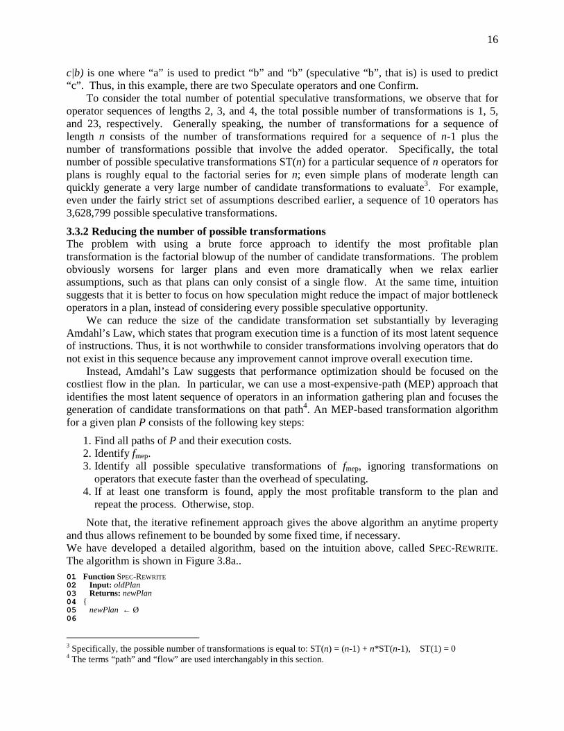
Note that, the iterative refinement approach gives the above algorithm an anytime property and thus allows refinement to be bounded by some fixed time, if necessary. We have developed a detailed algorithm, based on the intuition above, called SPEC-REWRITE. The algorithm is shown in Figure 3.8a.. 01 Function SPEC-REWRITE 02 Input: oldPlan 03 Returns: newPlan 04 { 05 newPlan ← Ø 06

3 Specifically, the possible number of transformations is equal to: ST(n) = (n-1) + n*ST(n-1), ST(1) = 0 4 The terms “path” and “flow” are used interchangably in this section.

17

07 do 08 newMep ← Ø 09 bestSpeedup ← 1 10 planPaths ← GET-ALL-PATHS (oldPlan) 11 mepInfo ← GET-MEP-INFO (planPaths) 12 13 foreach operator op ∈ mepInfo.mep 14 lhsTime ← GET-LHS-TIME (op, mepInfo.path) 15 rhsTime ← GET-RHS-TIME (op, mepInfo.path) 16 opTime ← CALC-OPERATOR-EXECUTION-TIME (op) 17 opOverheadTime ← (2 * per-tuple-overhead) * GET-AVERAGE-NUMBER-TUPLES-PROCESSED(op) 18 newMepTime ← lhsTime + MAX (opTime, rhsTime) + opOverheadTime 19 candSpeedup ← mepInfo.time / newMepTime 20 if candSpeedup > bestSpeedup then 21 newMep ← GENERATE-TRANSFORM-PATH(mepInfo.mep, op, op.previousOp, op.nextOp) 22 bestSpeedup ← candSpeedup 23 endif 24 end 25 26 if bestSpeedup > 1 then 27 if newPlan == Ø then 28 newPlan ← oldPlan 29 endif 30 newPlan ← REPLACE-PATH(newPlan, mepInfo.mep, newMep) 31 endif 32 33 while newMep != Ø 34 35 return newPlan 36 }

Figure 3.8a: The SPEC-REWRITE algorithm

To gather information about the current MEP, the SPEC-REWRITE algorithm calls the helper function GET-MEP-INFO, shown in Figure 3.8b. It returns an object called mepInfo that contains information on the most expensive path, including the cost of that path. This function is called during each iteration of plan transformation to locate which flow is the primary plan bottleneck. 01 Function GET-MEP-INFO 02 Input: planPaths 03 Returns: mepInfo 04 { 05 mepInfo ←new MepInfo 06 07 mepInfo.mep ← Ø 08 mepInfo.mepCost ← Ø 09 10 foreach path p ∈ planPaths 11 curCost ← 0 12 foreach operator op ∈ p 13 curCost ← curCost + CALC-AVERAGE-OPERATOR-EXECUTION-TIME(op) 14 end 15 if mep=∅ or curCost>mepCost then 16 mepInfo.mep ← p 17 mepInfo.mepCost ← curCost 18 endif 19 end 20 21 return mepInfo 22 }

Figure 3.8b: The GET-MEP-INFO helper function

To optimize the transformation of the MEP, the SPEC-REWRITE algorithm in Figure 3.8a uses the GET-LHS-TIME and GET-RHS-TIME functions to calculate the cost of the left-hand-side (LHS) and right-hand-side (RHS) of each speculation opportunity considered. For example, in the transformed CarInfo plan in Figure 3.6, consideration of the Speculate operator after the first wrapper operator would involve calculating the costs of the LHS – the time it takes to execute the Edmunds wrapper operator – and the cost of the RHS – the time it takes to execute the rest of

18

the plan. The best possible outcome is for the LHS cost and the RHS cost to be equal, which would enable correct speculation about the LHS to reduce the execution time of the original path by half (the maximum possible per speculation opportunity).

Note that the SPEC-REWRITE algorithm also accounts for the overhead of speculation. In particular, opOverheadTime is based on the per-tuple overhead, the additional time required per-tuple for context switching and speculation/confirmation processing, multiplied by the number of tuples usually seen by that operator. The per-tuple overhead is multiplied by 2 in the SPEC-REWRITE algorithm to account for the overhead associated with both Speculation and Confirmation per tuple. In addition to the algorithm taking into account overhead, performance degradation is also addressed by use of thread priorities, as discussed in section 3.1.2.

3.4 Experimental results5 To measure the impact of speculative plan execution on the information gathering process, we conducted experiments on a set of typical Web information agent plans. The goal of these experiments was to discover how useful the technique would be for the types of information integration plans that are common to Internet information gathering.

These experiments were conducted using Theseus, a streaming dataflow execution system for information agents (Barish and Knoblock, 2005). The Theseus plan language supports a Wrapper operator, as well as standard relational operators (Select, Project, etc.), and some additional operators for further types of data transformation, monitoring, and remote communication. These additional operators support the e-mailing data gathered, the scheduling agent plans, and the transformation to/from XML from/to relations.

Theseus was modified to support the automatic transformation of plans using the SPEC-REWRITE algorithm. In addition, Theseus was instrumented to count the average number of tuples per operator, per transaction as well as the average time it took to process each tuple. Using these numbers, Theseus iteratively transformed the MEPs in each plan, until no further transformations were possible (or profitable). For the second and successive runs, Theseus issued predictions using data acquired from past executions. It also collected source/target data for each speculative opportunity in order to improve its recall and precision for future runs.

3.4.1 Web agent plans To measure the utility of speculative execution on online information gathering, we looked at how the technique affected the performance of five different types of Web agent plans that integrate information between multiple Internet sources. These plans included:

• CarInfo: The main example, introduced in Section 1. • RepInfo: An agent described in (Barish and Knoblock 2002) that allows users to

specify an U.S. nine-digit zip code to query multiple Web sources that identify the set of corresponding U.S. federal congressional members (House and Senate), along with funding charts and recent news corresponding to each member.

• TheaterLoc: An agent that combines restaurant and theater data for a particular city and dynamically generates a map that plots their locations (Barish et al. 2000).

• FlightStatus: An agent described in (Ambite et al. 2002) that queries the status of a particular flight, and then e-mails the user/hotel with updates as necessary.

• StockInfo: An agent that takes a particular company name, identifies the stock symbol associated with it, locates profile information on that company, finds out

5 Data from our experiments can be found at http://www.isi.edu/integration/data/theseus/aij07data.html

19

what industry sector that company is in, identifies the largest competitor (based on market capitalization) and retrieves a chart that compares the 1 year performance of that competitor with the input company and the sector.

The details for each of these plans can be found elsewhere (Barish, 2003). Table 3.2 summarizes the original number of operators for each plan and the number of Speculate operators added after transformation for speculative execution.

AgentOriginal

number of operators

Speculate operators

addedCarInfo 7 3RepInfo 8 4

TheaterLoc 5 2FlightStatus 8 1StockInfo 7 7

Table 3.2: Summary of agent plans and resulting transformations

3.4.2 Example plan transformation To better illustrate the details of plan transformation using SPEC-REWRITE, we describe optimizing the real CarInfo plan, using actual operator execution times. In practice, the initial run of this plan took 6900 seconds and yielded the operator execution times shown in Table 3.3.

Operator Time (ms)

Join 10

Select 153

Wrapper (NHTSA) 359

Wrapper (Consumer Guide - Summary) 1912

Wrapper (Consumer Guide - Full Review) 2175

Wrapper (Consumer Guide - Search) 1478

Wrapper (Edmunds) 812

Total 6900

Table 3.3: Operator execution times in CarInfo

From this, the path execution times shown in Table 3.4 were calculated.

Path Path operators Time (ms)

P1 Edmunds + Select + NHTSA + Join 1334

P2 Edmunds + Select + CG-Search + CG-Summary + CG-Full + Join 6900

Table 3.4: Path execution times in CarInfo

The SPEC-REWRITE algorithm then used the above statistics to transform the plan for speculative execution. It first determined that the MEP of the plan was path P2. Initially, the most profitable operator to speculate about was the Consumer Guide Search wrapper. Parallelizing its execution through speculation with operators on the MEP leading up to it theoretically saved just over 1900ms (assuming 100% correct predictions). Note that even though the Consumer Guide Full Review wrapper took longer, parallelizing its execution with the rest of the plan would save little time, since only a very fast Join follows. By continuing with the algorithm, the original MEP was reduced further by speculating about both the Consumer

20

Guide Summary wrapper and Edmunds wrapper. In short, the algorithm transformed the plan so that instead of only two long parallel paths (as in Table 3.4), there were now many short parallel paths, as shown in Table 3.5.

Path operators Estimated Time (ms)

Edmunds + Spec + Confirm 1012

Spec + Select + NHTSA + Join + Confirm 669

Spec + Select + CG-Search + Spec + Confirm 1878

Spec + Select + Spec + CG-Summary + Spec + Confirm 2412

Spec + Select + Spec + Spec + CG-Full + Join + Confirm 2685

Table 3.5: Path execution times after transformation for speculative execution

Thus, the estimated execution time of the plan would be equal to the new MEP, the {Spec, Select, Spec, Spec, CG Full, Join, Confirm} path, 2685ms. This represents a speedup of (6900/2685 =) 2.57 over the original streaming dataflow plan, in terms of time to first tuple.

3.4.3 Overall results We compared the performance of normal execution to speculative execution for all five agent plans, focusing specifically on the speedups associated with the time to first and last tuple. When comparing normal execution to speculative execution, we looked at three cases of speculative execution:

• Optimistic: 100% correct • Average: 50% of the predictions (from all predictors) made were correct • Pessimistic: none of the predictions made were correct

By “percent correct”, we are referring to recall. For example, in the “50% correct” case, if the answer was (A, B), our 50% correct prediction might yield (A, C, D). We chose to measure these three cases of speculative execution to show the impact of prediction quality on plan speedup, while holding the speculative overhead constant. Figures 3.9a and 3.9b show the average performance at different levels of recall. Figure 3.9a shows the effect of speculative execution on the time to first tuple (start of output), while Figure 3.9b shows the impact on the time to the final tuple (end of output). The resulting average speedups for each of the plans, for both the 100% and 50% cases, are shown are shown in Figures 3.10a and 3.10b.

3.4.4 Discussion There were two interesting findings worth noting from the Web information gathering

results. The first was that speculative execution reduced average execution time significantly for CarInfo, RepInfo, TheaterLoc, StockInfo, and less significantly for FlightStatus. Clearly, this difference in the impact of speculative execution has to do with two factors: (a) the number of binding patterns between Wrapper operators in plan and (b) the latency of the sources used.

For example, the StockInfo plan had an MEP parallelizable to a degree of seven. Correspondingly, its average speedup was just under 4. This difference is likely due to the overhead of speculation. The same is true for CarInfo and RepInfo, which had MEPs parallelizable up to 3 and 4, respectively, and yielded average speedups of 2 and 2.5. In contrast, the maximum possible speedup for FlightStatus – if the sources were equally latent – was 2.0. However, since one of the sources (the U.S. Naval Time source) was very fast, execution time was dominated by the slower source (Delta airlines).

21

01000200030004000

5000600070008000

CarInfo RepInfo TheaterLoc FlightStatus StockInfo

Tim

e to

firs

t tu

ple

(ms)

No speculation

100% correct

50% correct

0% correct

Figure 3.9a: Execution time (time to first tuple)

0

1000

2000

3000

4000

5000

6000

7000

8000


Tim

e to

last

tup

le (m

s) No speculation

100% correct

50% correct

0% correct

Figure 3.9b: Execution time (time to last tuple)

0.000.501.001.502.002.503.003.504.004.50


Sp

eed

up

100% correct

50% correct

Figure 3.10a: Speedup (first tuple)

0.00

0.50

1.00

1.50

2.00

2.50

3.00

3.50

4.00

4.50


Sp

eed

up

100% correct

50% correct

Figure 3.10b: Speedup (last tuple)

22

A second notable finding was the difference in speedups between first and last tuple as a function of accuracy. For example, when 100% are correct, we see that the speedups of the time to first and the time to last tuple due to speculative execution roughly correspond. Consider CarInfo, where the first tuple and last tuple speedups were 1.98 and 1.76, respectively, a standard deviation of 0.16. However, when some predictions are incorrect, there were significant differences between first and last tuple speedups. For example, the CarInfo first and last tuple speedups for the 50% scenarios were 1.80 and 1.24, respectively, a standard deviation of 0.39.

The difference in deviations can be explained by the fact that, when correctness was less than 100%, one or more tuple(s) will have required traveling through the normal path of execution – that is, since confirmation failed at an earlier stage, some tuples needed to pass through some or all of the plan. However, minor speedups on the last tuple were still possible because (a) execution was more “spread out” (smaller groups of tuples required concurrent processing by Wrapper operators) and (b) although speculation failed some percentage of the time, it was rare that a tuple which failed but was corrected in the middle of the plan, failed again at a later point in the plan. Meanwhile, note that the speedups on the first tuple remained high (though there was some minor impact). This is because 50% of the predictions were correct – thus, some tuples predicted (and those derived from those tuples) did not require correction.

Finally, for purposes of clarity, it is useful to revisit the definitions of “optimistic” and “average” in the experiments. Note that for cascading speculation, the “optimistic” case assumed that all predictors in the modified plan are 100% correct in their predictions, all of the time. In contrast, the “average” case assumed that all predictors are 50% correct. This is equivalent to having said that (a) the plan input data is repeated 100% (or 50%, in the average case) of the time and that (b) no generalization (such as learning, discussed below) is performed. This means that, to an extent, the boundaries can be viewed as somewhat “over optimistic” and “over pessimistic”, depending on the application. Nevertheless, these assumptions allow us to get a sense for the impact of speculative execution given varying degrees of accuracy, and underscore the importance of making good predictions during speculative execution.

4. Learning Value Predictors The challenge of value prediction is to leverage knowledge about the set of past hints when making a prediction about a new hint. More specifically, the goal is to use some source tuple h as hint for issuing a predicted target tuple v. One approach to value prediction is to simply cache the association: we can note that particular hint hx corresponds to a particular target vy so that future receipt of hx can lead to prediction of vy. Caching is one simple and safe solution to the problem of value prediction. It requires no new algorithms and can be applied to any value prediction opportunity.

However, since the type of speculative execution that we have described occurs at the plan level, where the values being predicted are related tuples of data, there are often opportunities where it is possible to do much better. For example, in the CarInfo plan, the full review URL is simply just a transformation of the summary URL. We would like to learn this transformation function because it would enable us to make predictions even when evaluating new hints, ones which are not associated with a prior prediction. In addition, this type of predictor would also be smaller and bounded in its space requirements (i.e., storage of the function).

In this section, we introduce an approach to value prediction that combines caching with the techniques of classification and transduction. The resulting predictors learned are not only capable of both predicting values based on recurring past hints, but are also capable of making

23

predictions for new hints and synthesizing new predictions if necessary. As a result, the predictors can issue predictions more often. Asssuming the predictions are correct, this leads to better average plan speedups.

4.1 Value prediction strategies There are several potential methods that can be used to predict values, each differing in terms of their design complexity, space efficiency, and predictive capabilities. The last metric is especially important because better predictions at runtime translate into better speedups. To better compare methods of prediction, there are three scenarios to consider:

• Predictions of past values based on recurring hints: Given the past association of an input with an output, future receipt of that prior input can be treated as a hint hxi justifying prediction of that prior output value vyi. More compactly, this can be described as the case where (vyi | hxi).

• Predictions of past values based on new hints: In cases where a many-to-one or many-to-many relationship exists between hints and predictions, receipt of a new hint hxq ∈ H, where H = {hx1..hxm} and q > m can lead to a prediction vyi ∈ V, a previously collected set of predictions V = {vy1...vyn}, where 1 ≤ i ≤ n. Equivalently, this is the case (vyi | hxq).

• Predictions of novel values based on new hints: In cases where it can be observed that (vyi | hxi) and that vyi = F(hxi), we can learn function F and therefore be able to compute a prediction for some new hxj ∉ H, specifically to compute F(hxj) = vyj. Thus, this is the case (F(hxj) | hxj).

In this section, we discuss three strategies for value prediction – caching, classification, and transduction – and evaluate their accuracies with respect to these three categories.

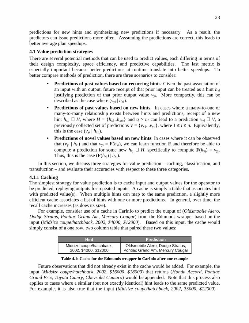
4.1.1 Caching The simplest strategy for value prediction is to cache input and output values for the operator to be predicted, replaying outputs for repeated inputs. A cache is simply a table that associates hint with predicted value(s). When multiple hints can map to the same prediction, a slightly more efficient cache associates a list of hints with one or more predictions. In general, over time, the recall cache increases (as does its size).

For example, consider use of a cache in CarInfo to predict the output of (Oldsmobile Alero, Dodge Stratus, Pontiac Grand Am, Mercury Cougar) from the Edmunds wrapper based on the input (Midsize coupe/hatchback, 2002, $4000, $12000). Based on this input, the cache would simply consist of a one row, two column table that paired these two values:

Hint Prediction

Midsize coupe/hatchback, 2002, $4000, $12000

Oldsmobile Alero, Dodge Stratus, Pontiac Grand Am, Mercury Cougar

Table 4.1: Cache for the Edmunds wrapper in CarInfo after one example

Future observations that did not already exist in the cache would be added. For example, the input (Midsize coupe/hatchback, 2002, $16000, $18000) that returns (Honda Accord, Pontiac Grand Prix, Toyota Camry, Chevrolet Camaro) would be appended. Note that this process also applies to cases where a similar (but not exactly identical) hint leads to the same predicted value. For example, it is also true that the input (Midsize coupe/hatchback, 2002, $5000, $12000) –

24

which differs from the first hint only on the minimum price – returns the same result as the first hint. If we now take all three instances and store them in the cache, the result is Table 4.2.

Hint Predictions




Honda Accord, Pontiac Grand Prix, Toyota Camry, Chevrolet Camaro



Table 4.2: Cache for Edmunds based on three examples

From these examples, it should be clear that caching is limited in that it can only respond to past hints. Furthermore, the minimum size of the cache required to store Table 4.2 is 184 bytes (counting only the unique data values needing storage) plus the data required to store information about the structure of the cache. However, from the examples seen, storing all of this data is not necessary – the same predictions can be made if we store only the key parts of information that distinguish one prediction from the others. We now describe alternative techniques to caching that can also be used for value prediction.

4.1.2 Classification Classification involves extracting knowledge from a set of data (instances) that describes how the attributes of those instances are associated with a set of target classes. Given a set of instances, classification rules can be learned so that recurring instances can be classified correctly. Once learned, a classifier can also make reasonable predictions about new instances, even instances that are a combination of attribute values which had not previously been seen. The ability for classification to accommodate new instances makes it a useful method of value prediction for speculative plan execution because, unlike caching, classification rules allow predictions to be made about new hints. A number of classification techniques exist (Mitchell, 1997; Duda et al., 2001).

As an example, consider again the prediction of the make and model of a car in the CarInfo plan. It turns out that Edmunds returns the same answer (Oldsmobile Alero, Dodge Stratus, Pontiac Grand Am, Mercury Cougar) for the criteria (Midsize coupe/hatchback, 2002) that also include any minimum price of $9912 or less and any maximum price of $11944 or more. This explains why the third hint in the example above, which had a minimum price of $5000, returned the same answer as the first. Thus, we see that in the case of the Edmunds wrapper, multiple search criteria can be associated with the same result.

Intuitively, we know that certain features of the hint will always lead to a different result than previous hints. For example, if we had altered the type or class of car, we know that we would not get the same set of results returned (and, in fact, we do not). However, intuition also suggests that there are ranges of prices that will return the same result of (Oldsmobile Alero, Dodge Stratus, Pontiac Grand Am, Mercury Cougar), but we do not know exactly what those ranges are. More important is the issue of encoding this knowledge into a predictor. Unlike classifiers, elementary caching approaches do not support any way to express rules under which hints can map to certain predictions.

Given a set of examples, a classifier can be used to learn rules for prediction that are based on features of the hint. The basic idea involves calculating the information gain that hint

25

attributes provide in terms of determining an association to a particular target class (the prediction). The more closely associated a particular feature of a set of training instances is with the target classes for each of those instances, the better that feature is at classifying the instances. For example, when considering the examples described in the caching section above, a decision tree classifier like C4.5 (Quinlan 1986) could induce the following rules:

min ≤≤≤≤ 5000: Oldsmobile Alero, Dodge Stratus, Pontiac Grand Am, Mercury Cougar

min>5000: Honda Accord, Pontiac Grand Prix, Toyota Camry, Chevrolet Camaro

When presented with an instance previously seen, such as (Midsize coupe/hatchback, 2002, $4000, $12000), both the cache and the classifier would result in the same prediction. However, when presented with a new instance, such as (Midsize coupe/hatchback, 2002, $4500, $12000), the cache would be unable to make a prediction whereas the classifier would issue the correct prediction. Note that even when classification leads to an errant prediction, the Confirm operator would prevent errant data from leaving the plan.

The decision tree above is also more space efficient than a cache for the same data. Recall that the cache requires storing at least 184 bytes. The decision tree above requires storing only 132 bytes (nearly a 30% improvement) plus the information required to describe tree structure and attribute value conditions (i.e., price < 18000). The space required for the tree structure varies based on the ratio of possible hints to possible predictions. The higher this ratio (i.e., many hints, few possible predictions), the less space required to describe the tree. However, as this ratio approaches 1, the classifier gradually emulates a typical association table. In extreme cases where the ratio is nearly 1, it will often be more efficient to use simple caching than to learn a classifier. In short, classifiers can often yield huge space savings and allow us to also make predictions about novel hints. However, there is a point of diminishing returns for some cases, especially as the number of possible predictions approaches the number of possible hints.

4.1.3 Transduction Transducers are finite state machines that transform input to output by using the former to iteratively proceed through a series of states that progressively produce the latter. One type of transducer is a string-to-string sequential transducer, defined by (Mohri 1997) as T = (Q, i, F, Σ, ∆, δ, σ), where Q is the set of states, i ∈ Q is the initial state, F ⊆ Q is the set of final states, Σ and ∆ are finite sets corresponding to input and output alphabets, δ is the state-transition function that maps Q x Σ to Q, and σ is the output function that maps Q x Σ to ∆*.

A more general type of subsequential transducer is the p-subsequential transducer which extends the definition of a sequential transducer by allowing the final state to include p additional output arcs. This simply allows the transducer to append on additional characters (i.e., a suffix). Transducers are used in many sub-disciplines of computer science, including natural language processing, where they have been applied to the problem of automatically translating a source string to a target string.

Value prediction by transduction makes sense for Web information gathering plans primarily because of how Web sources organize information and how Web requests (i.e., HTTP queries) are standardized. In the case of the former, Web sources often use predictable hierarchies to catalog information. For example, in the CarInfo example, the summary URL for the Dodge Stratus was http://cg.com/summ/20812.htm and the full review was at http://cg.com/full/20812.htm. Notice that the second URL contains the key piece of dynamic information (20812) found in the first URL. One could construct a transducer that extracts that

26

information from the first URL and combines it with other static data to yield the full review URL, as shown in Figure 4.1. By learning such a transducer, we can then predict future full review URLs for other summary URLs previously unseen. In addition to URLs, transducers can also be used to predict HTTP query parameters. For example, an HTTP GET query for the IBM stock chart is http://finance.yahoo.com/q?s=ibm&d=c. By exploiting the regularity of this URL structure, the system can predict the URL for the Cisco Systems (CSCO) chart. Our use of transducers here is thus similar to existing methods of extracting information from semi-structured sources (Ashish and Knoblock, 1997; Kushmerick 1997; Freitag 1998), with the additional point that we want to use the extracted information to generate a new predicted value. An important feature of our approach is that any transducer learned will always be 100% accurate with respect to the training data.

In this section, we define two new types of transducers that extend the traditional definition of p-subsequential transducers. The first is a high-level transducer, called a value transducer that constructs a predicted value based on the regularity and transformations observed in a set of examples of past hints and values. Value transducers build the predicted value through substring-level operations {Insert, Cache, Classify, Transduce}. Insert constructs the static parts of predicted values. Cache recalls past values associated with the hint key. Classify categorizes hint information into part of a predicted value. Finally, Transduce transforms hint information into part of a predicted value. Transduce uses a second type of special transducer, called a hint transducer, in which the operations {Accept, Copy, Replace, Upper, Lower} all function on individual characters of the hint and perform the same transformation as their name implies, with respect to the predicted value. The difference between the value transducer and the hint transducer is that the former coordinates the production of the prediction (possibly using the latter, as well as other higher level techniques) whereas the latter is simply a tool that may be used to extract out relevant information (such as the “20812” substring, in Figure 4.1) as part of the value transduction process.

To illustrate, consider the process shown in Figure 4.2, which can be applied to predicting the full-review URL in the CarInfo example. The figure shows two transducers. The upper one, the value transducer, performs high-level operations including the insertion of substrings and the call to a lower-level transduction process. The second transducer (in abbreviated form) is a hint transducer. The example shown uses the Accept and Copy operations to transform the hint value (http://cg.com/summ/20812.htm) into its proper point in the predicted value. In summary, the value transducer first builds the “http://cg.com/full/” part, the hint transducer is then applied

http://cg.com/summ/20812.htm

http://cg.com/full/20812.htm

To create full review URL:

1. Start with "http://cg.com/full/"2. Append the dynamic part of the

summary URL (e.g., 20812)3. Append ".htm"

1 2 3

Figure 4.1: Full review URL transduction is part extraction, part production

27

to fill in the dynamic part “20812” via copying it from the hint value, and finally the third value transducer operation appends the “.htm” suffix.

The key idea this example shows is that synthesis of a prediction can consist of several sub-operations. Some of these sub-operations, such as Insert, are independent of the hint value. Others, such as Transduce, Classify, and Cache are a function of the hint value. Together, both types of sub-operations enable values to be generated, even from never-before-seen hints.

Transducers lend themselves to value prediction because of the way information is stored by and queried from Web sources. They are a natural fit because URLs are strings that are often the result of simple transformations based on earlier input. Thus, for sources that provide content that cannot be queried directly (instead requiring an initial query and then further navigation), transducers serve as predictors that capitalize on the regularity of Web queries and source structure.

In terms of space efficiency, a learned transducer is generally very compact because what is learned is a set of transformation rules for the hint. For example, once the value transducer shown in Figure 4.2 is learned, it can be applied to all new hints. It should be noted that transducers in other areas of computer science, such as natural language processing, are not always compact and do grow as more examples are seen. In contrast, the types of transducers common to Web information gathering plans, in particular those useful for URL prediction, tend to be more like small functions. As a result, space demands typically remain fixed over time.

4.1.4 Comparison of techniques In this section, we have discussed three value prediction techniques: caching, classification, and transduction. Each has it advantages and disadvantages. Basic caching is simple, always works when given a recurring hint, but is useless when receiving new hints; it also has the worst space efficiency of the three. Nevertheless, it is a good alternative when no other learning algorithm can be applied.

Classification has better space efficiency and can deal with new hints, mapping multiple hints to values that have been previously ssen. Furthermore, if necessary, can roughly emulate a cache for cases where all hint features are equally good/bad in terms of prediction.

Transduction is the most space efficient of the three, is capable of dealing with new hints as well as making novel predictions, and is especially relevant for Web agent plans because of its applicability at predicting URLs. The only disadvantage to transduction is that it is not always relevant for all speculative opportunities (i.e., some predictions are associated with hints, not computed based on hints). Table 4.3 compares all techniques along the categories specified earlier including space efficiency.

Figure 4.2: Value transducer for the full-review URL in CarInfo

1 2

INSERTINSERTINSERTINSERT("http://cg.com/full/")

TRANSDUCETRANSDUCETRANSDUCETRANSDUCE(hint)

3

INSERTINSERTINSERTINSERT(".htm")

2a 2b

u:ACCEPTACCEPTACCEPTACCEPT /:ACCEPTACCEPTACCEPTACCEPT

ε:ACCEPTACCEPTACCEPTACCEPT

2c

ε:COPYCOPYCOPYCOPY

.:ACCEPTACCEPTACCEPTACCEPT

2d

ε:ACCEPTACCEPTACCEPTACCEPT ε:ACCEPTACCEPTACCEPTACCEPT

28

Strategy Predicts past values from past hints

Predicts past values from new hints

Predicts novel values from new

hints

Space efficiency: growth rate

Caching Yes No No Linear Classification Yes Yes No Sub linear

Transduction Yes Yes Yes Constant

Table 4.3: Comparing value prediction strategies

Note that while we have discussed three possible strategies, other strategies do exist. For example, one could use a more advanced form of caching, such as semantic caching (Dar et al., 1996; Adali et al., 1996), or an alternative function-learning algorithm to transduction. We focused on the three strategies above because they are easy to understand and demonstrate the key differences in the prediction scenarios introduced earlier.

4.2 A Unifying Learning Algorithm In this section, we present a set of algorithms that describe how to combine caching, classification, and transduction in order to generate efficient and accurate predictors. By combining all three strategies, there is an increase in the flexibility for prediction synthesis. For example, with the algorithms we present, it is possible to learn a predictor that synthesizes a new prediction through a combination of caching, classification, and transduction of the hint received.

4.2.1 Value Transducers Our approach to value prediction involves inducing a value transducer (VT) that describes how to generate a prediction from a hint, using sub-operations that include classification, transduction, and caching. To learn a VT for the speculative execution of information gathering plans, the following is required:

1. For each attribute of the answer tuple, identify a Static/Dynamic (SD) Template that distinguishes the static parts from dynamic parts of the target string by analyzing the regularity between values of this attribute for all answers.

2. For each static part, add an Insert arc to the VT. 3. For each dynamic part, determine if transduction can be used; if so, add a Transduce arc

to VT. 4. If no transducer can be found, classify the dynamic part based on the relevant attributes of

the hint and learn a classifier. 5. If classifier accuracy is at or above a predefined Threshold, add a Classify arc to the VT. 6. If the classifier accuracy is below Threshold (possible when one or more hint features are

continuous), build a cache of the data and add a Cache arc to the VT.

These steps are implemented in the algorithm LEARN-VALUE-TRANSDUCER, shown in Figure 4.3. The algorithm takes a set of hints, a set of corresponding answers, and returns a VT that fits the data. In this algorithm, learning a classifier can be achieved by decision tree induction (Quinlan, 1986). Learning the SD template and the hint transducer, however, requires unique algorithms. Note that, for purposes of simplification, parts of the LEARN-VALUE-TRANSDUCER algorithm assume correspondence between elements of two different lists (e.g., H and DA when calling LEARN-HINT-TRANSDUCER, H and DA when calling LEARN-CLASSIFIER, etc.).

29

01 Function LEARN-VALUE-TRANSDUCER returns ValueTransducer 02 Input: set of hints H, corresponding set of answers A 03 VT ← ∅ 04 tmpl ← LEARN-SD-TEMPLATE (A); 05 Foreach element e in tmpl 06 If e is a static element 07 Add Insert (e.value) arc to VT 08 Else if e is a dynamic element 09 DA ← the set of dynamic strings in A for this tmpl element 10 HT ← LEARN-HINT-TRANSDUCER (H, DA) 11 If HT != ∅ 12 Add Transduce (HT) arc to VT 13 else 14 CL ← LEARN-CLASSIFIER (H, DA) 15 acc = TEST-CLASSIFIER (CL, H, A) 16 If acc < Threshold 17 CH ← BUILD-CACHE (H, DA) 17 Add Cache (CH) arc to VT 18 Else 18 Add Classify (CL) arc to VT 19 Return VT 20 End /* LEARN-VT */

Figure 4.3: The LEARN-VALUE-TRANSDUCER algorithm

4.2.2 Learning string templates To identify a static/dynamic template, we first locate the static parts by comparing the target values to each other. Substrings of characters that all target values share are considered static parts. The dynamic parts of the template are the substrings of varying characters between two static parts (or the start and end of the template). Thus, each SD template will consist of an alternating sequence of static and dynamic parts.

To identify the static parts of a template, we first locate the common substrings in the set of target values. To do this, we first sort the set of strings by length in ascending order. We then find the common substrings between the first two strings, forming a template (we can use a special character to separate substrings). If a common template is found, we then find the common substrings between the template identified thus far and the successive strings. We continue until either we have exhausted the set of strings or the template is null (because we encountered a case where no common substrings are found).

For example, using the special character $ to separate common substrings in the template (and thus representing the dynamic part), and given the strings {foo.com?i=10&p=home, foo.com?i=20&p=rome, foo.com?i=21&p=nav}, we would first identify the template foo.com?i=$0&p=$ome. Using this and iterating to the next string, we find the template reduced to foo.com?i=$&p=$. This is the template we would return. The algorithm that implements this, LEARN-SD-TEMPLATE, is shown in Figure 4.4.

30

01 Function LEARN-SD-TEMPLATE returns Template 02 Input: set of strings S 03 S′ ← sort strings by length in ascending order 04 tmpl ← ∅ 05 Foreach i in 1..length(S′.length)-1 06 tmpl ← FIND-COMMON-SUBSTRINGS (tmpl, S′[i] ) 07 If tmpl == ∅ 08 break; 09 Endif 10 End 11 Return tmpl 12 End /* LEARN-SD-TEMPLATE */

Figure 4.4: The LEARN-SD-TEMPLATE algorithm

4.2.3 Learning hint transducers To learn a hint transducer, we also make use of template identification. However, instead of identifying an SD template that fits all answers, the algorithm identifies a template that fits all hints. That is, we try to identify hint regularity – for example, that all hints are prefixed with http://cg.com/summ/. Based on one of these templates, and the corresponding dynamic strings passed from the LEARN-VALUE-TRANSDUCER algorithm (line 9), the algorithm constructs a lower-level hint transducer that accepts the static parts of the hint string and performs character-level transformations (Accept, Copy, Replace, Upper, or Lower) on the dynamic parts. A sketch of the algorithm that implements this, LEARN-HINT-TRANSDUCER, is shown in Figure 4.5.

01 Function LEARN-HINT-TRANSDUCER returns HintTransducer 02 Input: the set of hint and result string pairs (H, R) 03 ht ← ∅ 04 htmpl ← FIND-COMMON-SUBSTRINGS (H) 05 Foreach H,R pair (h, r) 06 h′ ← extraction from h, based on htmpl, replacing each static character with the accept annotation A 07 hra ← alignment of (h′, r) based on string edit distance 08 Annotate hra with character level transformation required (e.g., Copy), ignoring previous A annotations 09 End 10 RE ← Build regular expression of hra values that summarizes annotations 11 If RE != ∅ 12 ht ← transducer based on RE that accepts static subsequences of H and transduces dynamic subsequences. 13 Endif 14 Return ht 15 End /* LEARN-HINT-TRANSDUCER */

Figure 4.5: The LEARN-HINT-TRANSDUCER algorithm

For example, suppose prior hints {“Dr. Tom Smith”, “Dr. Jane Thomas”} had corresponding observed values {“tom_s”, “jane_t”}. The algorithm would first identify the static part of the hints and rewrite the hints using the Accept operation, i.e., {AAAATom Smith, AAAAJane Thomas} where A refers to the operation Accept. It would then align each hint and value based on string edit distance and annotate with character level operations that reflect the transformation to the observed values, resulting in {AAAALCCRLDDDD, AAAALCCCRLDDDDD}. Next, it would identify common substrings to build the regular expression {A*LC*RLD*} fitting these examples and ensure that intermediate operations of indeterminate length (the A* and C* in this example) share a common character upon which they stopped. From this, a general predictive transducer can be constructed, a partial form shown in Figure 4.6. For purposes of describing this transducer in text form, we can abbreviate Figure 4.6 as {Athrough=<SP>, L, Cupto=<SP>, A, L} which means “accept through the first space,

31

lowercase the next character, copy successive characters until the next space, accept the space and then lowercase the next character.

To better illustrate how a predictor is learned with the LEARN-VALUE-TRANSDUCER algorithm, we describe how the second predictor in the CarInfo plan, which generates the ConsumerGuide summary URL, is learned. In this example, the source value is a tuple consisting of the make, model, and year of a car (from a list of cars returned by Edmunds). The target value to be predicted is the summary URL that is normally discovered by querying ConsumerGuide.com with the make, model, and year of the car.

It is important to note that the target value also includes the input attribute values - make, model, and year. That is, the target tuple has four attributes. The reason for this is that the Wrapper operator that queries ConsumerGuide.com normally performs a dependent join on the output from the source with the input data. However, this means that the LEARN-VALUE-TRANSDUCER algorithm will be used four times – once for each attribute – so that a hint results in four different value transductions in creating the predicted tuple.

Learning is continuous in the sense that it can be re-applied offline after each run. Continual learning is desirable because (1) it allows new predictions to be made and (2) to allow the predictors to be refined over time, as more examples have been collected. For purposes of example, suppose that the source and target examples shown in Tables 4.4a and 4.4b are observed by the system over successive runs and that learning/re-learning occurs after every run. We also note that our algorithm does not overfit because because what is deduced is common to all of a single vector of data (it does not get thwarted by other, irrelevant attributes).

Make Model Year Honda Accord 1999

Honda Accord 2000

GMC Sonoma 1997

Acura NSX 2000

Table 4.4a: The sequence of source examples (inputs to the ConsumerGuide search operator)

Make Model Year Summary URL Honda Accord 1999 http://cg.com/summ/2289.html

Honda Accord 2000 http://cg.com/summ/2289.html

GMC Sonoma 1997 http://cg.com/summ/2247.html

Acura NSX 2000 http://cg.com/summ/1997.html

Table 4.4b: The sequence of target examples (outputs from the ConsumerGuide search operator)

Let us now describe the learning as it would occur tuple by tuple. After the second run of the speculative CarInfo plan, only the first two tuples ((Honda, Accord, 1999), (Honda, Accord, 1999, http://cg.com/summ/2289.htm)) and ((Honda, Accord, 2000), (Honda, Accord, 2000,

Figure 4.6: Partial form of hint transducer for the names example

1 2

<SP>:ACCEPT:ACCEPT:ACCEPT:ACCEPT

ε:ACCEPT:ACCEPT:ACCEPT:ACCEPT

ε:ACCEPT:ACCEPT:ACCEPT:ACCEPT

3

ε:LOWER:LOWER:LOWER:LOWER

4

ε:COPY:COPY:COPY:COPY

ε:COPY:COPY:COPY:COPY

5

<SP>:ACCEPT:ACCEPT:ACCEPT:ACCEPT

6

ε:LOWER:LOWER:LOWER:LOWER

32

http://cg.com/summ/2289.htm)) would have been observed by the system. LEARN-VALUE-TRANSDUCER would then identify a VT for each attribute of the target tuple. As the algorithm specifies, the first step is to define a template and then, based on that template, possibly learn additional transducers or classifiers as necessary. Since two very similar examples are seen initially, the template for the target “make”, “model”, and “summary URL” attributes consists of only a single static element, the template abbreviated here as {Static}. As a result, the resulting VTs for make, model, and summary URL consist of only a single Insert operation.

However, since there is no common substring between the two target year examples, the template for that attribute is {Dynamic}. Next, the source tuple attribute values are compared against the target attribute values in order to possibly identify a valid hint transducer. The first target attribute value is the year “1999”. The smallest edit distance between any of the corresponding source attributes (Honda, Accord, 1999) and this year value is the source “year” attribute (also “1999”), which has a distance of zero. Next, a case-independent alignment is done between the two strings, the transducer {CCCC} is learned, and then the generalized form Transduce(year: C*) is retained. This transducer is then verified for the remaining examples: since it correctly produces “2000” from the corresponding source tuple (Honda, Accord, 2000) of the remaining example, the transducer is deemed valid and incorporated into the VT for the year attribute. Details about the complete set of VTs after the first run are shown in Table 4.5:

Attribute Value Transducer Make INSERT("HONDA") Model INSERT("ACCORD")

Year TRANSDUCE(year: C*)

Summary URL INSERT("http://cg.com/summ/2289.htm")

Table 4.5: VTs for the ConsumerGuide search predictor after two examples

After the next run, the system receives a third example: ((GMC, Sonoma, 1997), (GMC, Sonoma, 1997, http://cg.com/summ/2247.htm)). The predictors are once again re-learned, but this time the target “make”, “model”, and “year” attributes are refined. Because the common substrings for the strings (Honda, Honda, GMC) = ∅, a dynamic template is identified and a VT consisting of Transduce(make: C*) is learned. The templates for “model” and “year”, however, are a bit more complicated.

Because the common substring for (Accord, Accord, Sonoma) = “o”, the template for the “model” attribute is {Dynamic, Static, Dynamic}. Even though we intuitively realize that the correct VT for this attribute should be to simply copy all of the characters of the source “model” attribute, the limited number of examples seen temporarily suggest otherwise. Two hint transducers are learned. The first copies all characters from the source model attribute up to the first ‘o’. Next, an Insert operation inserts an “o” and then a second hint transducer accepts all of the source model characters through the “o” before copying the rest. In short, the fact that an “o” existed in all three examples temporarily made the transducer more complex than it needed to be. The same is somewhat true of the Summary URL attribute – since all examples thus far included a “22”, the system assumed that this substring should be present in all predictions. Table 4.6 shows the state of the VTs after three examples.

33

Attribute Value Transducer Make TRANSDUCE(make: C*)

Model TRANSDUCE(model: Cupto=[o]), INSERT("o"), TRANSDUCE(model: Athrough=[o], C*)


Summary URL

INSERT("http://cg.com/summ/22"), CLASSIFY(make, model, year), INSERT(".htm")

Table 4.6: VTs for the ConsumerGuide search predictor after three examples

Finally, the ((Acura, NSX, 1997), (Acura, NSX, 1997, http://cg.com/summ/1997.htm) example eliminates the static artifacts that affected both the “model” and “year” attributes, allowing the VTs to settle into their correct state. Table 4.7 shows the VTs for this predictor.

Attribute Value Transducer

Make TRANSDUCE(make: C*)

Model TRANSDUCE(model: C*)


Summary URL INSERT("http://cg.com/summ/"), CLASSIFY(make, model, year), INSERT(".htm")

Table 4.7: VTs for the ConsumerGuide search predictor after four examples

As this detailed example has shown, the value predictors learned rely on a hybrid of techniques to predict likely target tuple values. Each predictor consists of VTs that may combine Insert, Transduce, and Classify operations as necessary. Note that Transduce is a character-level transduction, as opposed to the higher level transduction done by the VT that includes it. Predictors can be learned after only two examples, although as our example predictor has revealed, the final form of the value transducers for a predictor may require a few more examples in order to correctly identify the regular (i.e., static) and irregular (i.e., dynamic) parts.

4.3 Experimental results To measure the effectiveness of the approach, we conducted experiments on a representative set of typical Web agent plans modified for speculative execution (a subset of the plans described earlier). The goal was to compare the benefits of strictly caching versus the benefits of the learning the hybrid predictors we have introduced. Specifically, the goal was to verify that our approach to learning value predictors resulted in:

• Improved accuracy: Predictions based on classification and/or transduction makes it possible to speculate on recurring as well as new hints, and support the issuing of recurring or novel predictions.

• Improved space-efficiency: Since the predictors we learn are more like functions that describe a general process for producing a prediction from a hint, their storage does not necessarily increase linearly as the number of examples seen increases. In contrast, strictly caching predictors do grow linearly since they capture the association of past source tuples with past target tuples.

34

• Faster average agent performance: Learning hybrid predictors that combine classification, transduction, and caching allow us to obtain faster agent performance, on average, even when dealing with new hints or when needing to issue novel predictions.

We now describe the details of the experimental setup and the results found using the CarInfo and RepInfo agent plans described in Section 3. We also add a new example, the PhoneInfo agent6. We describe RepInfo and PhoneInfo in greater detail, below, since the discussion that follows will refer to specific operators and instances of speculation. Furthermore, we summarize our experimental setup in Table 4.8, showing the plans, the number of operators, and the original average execution time.

AgentOriginal

number of operators

Number of speculate operators

added

Original time to first tuple (ms)

Original time to last tuple (ms)

CarInfo 7 3 3296 5201RepInfo 8 4 4440 5008

PhoneInfo 4 3 4910 4910 Table 4.8: Summary of agent plans used in experiment

4.3.1.1 RepInfo This agent uses Congress.org (http://www.congress.org) to identify the congressional members based on zip code, Yahoo News (http://news.yahoo.com) for headlines about each member, and Open Secrets (http://www.opensecrets.org) for funding charts for each member. Figure 4.7a shows the original RepInfo plan while Figure 4.7b shows the plan modified for speculative execution. Note that querying both Congress.org and the chart from Open Secrets requires navigating from links derived from an initial query – thus, interleaved navigation is required in order to obtain an answer during plan execution.

6 Note that our experiments look at a relevant subset of the plans described earlier. Our goal was to demonstrate the potential efficiency and accuracy benefits of our approach to value prediction.

W

J

SW

W

SPEC

CONFIRM

SPEC

W

WSPEC

WSPEC

Figure 4.7b: The modified RepInfo agent plan

WRAPPEROpen Secrets

Search

nine-digit

zip code

WRAPPEROpen Secrets

Info

WRAPPEROpen Secrets

Funding

WRAPPERCongress.org

Search

JOIN

SELECTtitle =

'Rep' or 'Sen'

WRAPPERYahoo

News

Rep

info

WRAPPERCongress.org

Info

Figure 4.7a: The RepInfo agent plan

35

4.3.1.2 PhoneInfo The PhoneInfo agent returns demographic information for the geographic location of a particular phone number. The agent takes any phone number and first does a reverse lookup of that number using the Verizon SuperPages (http://www.superpages.com) service. The returned state is then used to query a U.S. Census site (http://quickfacts.census.gov) in order to obtain demographic data (e.g., population trends, average income) for that location. During the gathering of demographic data, navigation is required from a link on the initial “state summary” page to a subsequent “demographic details” page. The original plan for PhoneInfo is shown in Figure 4.8a and the same plan transformed for speculative execution is shown in Figure 4.8b. The PhoneInfo agent is added to the set of plans tested because it demonstrates classification with numeric hint attributes, specifically, the determination of state based on area code.

4.3.2 The learning cycle After each agent plan was modified for speculative execution, successive runs of the transformed plan predicted data when possible and always gathered more examples so that the predictors learned could be improved. Thus, for the second and future runs, prediction became possible more often, as more examples had been observed and processed by the system.

All learning was done offline. Generally, learning was possible every k runs, where k was customizable. Prior to each interval of k, data would be collected by the system. These represent the set of training examples which would be later fed to the learning algorithm. After every kth run, the system would use the training data to re-learn all of the predictors.

The LEARN-VALUE-TRANSDUCER algorithm was successfully applied to each opportunity in each plan, yielding value transducers that predicted values based on hint transduction, classification, or caching. Table 4.9 gives names to each predictor and summarizes the primary technique used in generating predictions from hints:

Overall, Table 4.9 shows three important things. It shows that the learning algorithms successfully learned a predictor for each speculative opportunity (i.e., there was never a time that the algorithm could not learn a predictor). Second, the table shows that the algorithms resulted in value transducers based on different primary methods of prediction, as a function of past hint/value relationships observed. Third, even when transduction was impossible and classification was not relevant (i.e., hint consisted of only a single, non-continuous feature), caching could still be used. In short, the table shows how our approach to learning value predictors allows either transduction, classification, or caching to be applied to a given speculative opportunity, based on the nature of relationship between the source and target data.

WW SPEC CONFIRMWSPECWSPEC

Figure 4.8b: Speculative version of PhoneInfo

WRAPPERCensus.gov

Demographic info

phone

number

WRAPPERSuperPages.com

Search

Demographic

information for

geographic location of

phone number

WRAPPERCensus.gov

State search

WRAPPERCensus.gov

State info

Figure 4.8a: The Phone Info agent plan

36

Predictor Plan Hint (source value) Prediction (target value) Predictor type

Car-List CarInfo User car preferencesList of matching cars from Edmunds.com

Classification

Car-Summary CarInfo Car make, model, and year ConsumerGuide.com summary page Classification

Car-Full CarInfoConsumerGuide.com summary page

ConsumerGuide.com full review page Transduction

Rep-List RepInfo User 9-digit zip codeList of federal representatives from Congress.org

Classification

Rep-Cand RepInfoURL to federal representative bio

Representative name and title Caching

Rep-Summary RepInfoRepresentative name and title

Open Secrets summary page URL Caching

Rep-Graph RepInfoOpen Secrets summary page URL

Open Secrets funding graph URL Transduction

Phone-State PhoneInfo User phone numberState of origin, as identified by Superpages.com

Classification

Phone-Summary PhoneInfo StateCensus summary page URL located at QuickFacts.census.gov

Caching

Phone-Detail PhoneInfoCensus summary page URL

Census demographic details page URL Transduction

Table 4.9: Summary of predictors learned

4.3.3 Measurements of predictor accuracy One of our goals is to compare the accuracy of predictors learned via the algorithms presented in this section versus predictors that operate strictly by cached data. We define accuracy as follows. For a given prediction consisting of a set of one or more tuples, recall is the number of tuples in that prediction set that are in the answer set, divided by the number of tuples in the answer set. Precision is the number of tuples in the prediction set that are also in the answer set, divided by the number of tuples in the prediction set. Thus, if a predictor generates (A, B, C, D) when the answer is (A, X, Y), the recall is 33%, the precision is 25%. As usual, high precision or high recall alone is not a good measure of the utility of a predictor; the combination of both (e.g., an F-measure) yields a better characterization.

In comparing the accuracy of predictors, it is important to assess the accuracies with respect to the three prediction scenarios described earlier: the cases of the (I) recurring hint / recurring prediction, (II) novel hint / recurring prediction, and (III) novel hint / novel prediction. Note that not all of these scenarios are relevant to each speculative opportunity. For example, there is no case (II) for the Carfull predictor because each unique summary page corresponds to a unique full review URL. Similarly, there is no case (III) for the Carsummary predictor because more than one car could correspond with the same summary page. We now describe the accuracy of the predictors in Table 4.9 for each of the prediction scenarios. When learning each predictor, instances were drawn from typical distributions for that domain; for example, instances for RepInfo were drawn from a list of addresses of individuals that contributed to presidential campaigns (obtained from the FEC) – a distribution that closely approximates the U.S. geographic population distribution. Similarly, the phone numbers used in PhoneInfo came from a distribution of numbers for common last names.

Case I: Recurring hints, recurring predictions Regardless of what type of predictor (transduction, classification, or caching) was settled upon by the LEARN-VALUE-TRANSDUCER algorithm, recall and precision with respect to recurring hints was as high as desired. For caching predictors (such as Phonesummary), this is obviously

37

because we stored a table of past hints and corresponding past results. Future prediction based on this data is simply a matter of looking up the result associated with the recurring hint.

For classification and transduction predictors, the LEARN-VALUE-TRANSDUCER

algorithm ensures that accuracies up to Threshold are maintained. Choosing a classification or transduction based predictor did not result in sacrificing the ability to respond to recurring hints when compared to caching. Threshold can be fixed or it may vary over time, with factors such as cache size or information about the likelihood of hint recurrence possibly becoming relevant. For example, if one knows that hints will never repeat, a classifier that cannot be completely validated using its own training data may still be an acceptable solution (because caching will do no better). However, for simplicity in our experiments, Threshold was set at 100%.

Case II: New hints, recurring predictions When presented with new hints, simple caches cannot issue predictions, even if they map to recurring hints. This is because caching associates distinct source values with target values and is not designed to infer anything about a new source value.

In contrast, classifiers can handle situations where there is a many-to-one mapping between hints and predictions and thus allow reasonable predictions to be made from a new hint. In Table 4.9, Carsummary, Replist, and Phonestate are such predictors. We measured the recall of on previously unseen hints, as the number of training examples increased. The results were based on averaging a 10-fold cross-validation sample of the data in each case. Figure 4.9 shows the results for each of the classifiers Carsummary, Replist, and Phonestate.

The figure shows that, generally, as the number of training examples increased, the precision on unseen examples also increased for each of the predictors. Note that the Phonestate classifier performance improves significantly just after 600 examples. This appears to be due to the fact that the precision of the classifier for a few of the larger states (like California, Florida, New York, and Texas) improves significantly around this point. Since instances from larger states appear more often then file (a representative sample), precision correspondingly improves.

Case III: New hints, novel predictions The approach we present also allows certain predictors to issue novel predictions for new hints. Such opportunities occur when the cardinality between source and target value is one-to-one and

Figure 4.9: Recall of Carsummary, Replist, and Phonestate classifiers

0.00%

10.00%

20.00%

30.00%

40.00%

50.00%

60.00%

70.00%

80.00%

90.00%

100.00%

200 400 600 800 1000

Number of new examples

Rec

all

Car-summary

Rep-list

Phone-state

38

when the target value can be produced through some type of hint attribute value transduction. In Table 4.8, only the Carfull, Repgraph, and Phonedetail predictors rely purely on hint transduction. In contrast, a predictor like Carsummary (which computes the summary URL from search criteria) is not in this category; it must see a value before being able to issue that value again as a prediction.

We have previously described the input data to the problem (the hint and target tuples) for the Carfull predictor. In Table 4.10a, we show examples of the input data for the other two predictors. The data extracted and then used in the generation of output is presented in bold, with underline (e.g., the “06”) in the first Phone-detail example.

Input Output

Phone-detailhttp://quickfacts.census.gov/qfd/states/06000.html

http://factfinder.census.gov/servlet/ACSSAFFFacts?_event=Search&_lang=en&_sse=on&geo_id=04000US06&_state=04000US06

http://quickfacts.census.gov/qfd/states/32000.html

http://factfinder.census.gov/servlet/ACSSAFFFacts?_event=Search&_lang=en&_sse=on&geo_id=04000US32&_state=04000US32

Rep-graphhttp://www.opensecrets.org/politicians/summary.asp?cid=N00007665

http://www.opensecrets.org/politicians/sector_img.asp?id=N00007665&cycle=2006

http://www.opensecrets.org/politicians/summary.asp?cid=N00009677

http://www.opensecrets.org/politicians/sector_img.asp?id=N00009677&cycle=2006

Table 4.10a: Sample data used by Phone-detail and Rep-graph predictors

Once learned, these transducers have accuracies of 100%. They essentially capture a function and then perform that function on all new hints. The only time when these transducers make mistakes are when too few examples have been seen and LEARN-VALUE-TRANSDUCER identifies an incorrect template. For example, learning that the first three attributes of the Phonestate predictor were direct copies of input attribute values (i.e., the definition of a dependent join) required more than two examples for some of the attributes because an common substring “artifact” was caused by learning based on a fewer number of examples.

To understand the difficulty of identifying the correct transducer, we investigated how many examples were required (on average) to learn the transducers Carfull, Repgraph, and Phonedetail. In doing so, we first identified the correct transducer for each case. Then, using 10 different randomized orderings of sample source/target values, we averaged the number of examples required before the correct transducer was learned. Table 4.10b shows these results.

PredictorAvg number of

examples requiredCar-Full 3

Rep-Graph 8Phone-Detail 3

Table 4.10b: Average number of examples required to learn Carfull, Repgraph, and Phonedetail

4.3.4 Measurements of predictor space-efficiency In addition to comparing the approach described in this paper to caching in terms of accuracy, we also compared the space efficiency of the two techniques. Specifically, we measured the space efficiency of three classification-based predictors (Carsummary, Replist, and Phonestate) and three transduction-based predictors (Carfull, Repgraph, and Phonedetail) as well as the space required by strictly caching predictors for the same data. The process involved forming the predictor

39

based on a set of training data and then exporting the structure to the file system for future runs. The space measured was the total number of bytes required by the data structure.

Table 4.11a shows the results for each classification-based predictor, its cache counterpart, and the number of training instances seen by each prior to the exporting of the data structure. In addition to a bytes-to-bytes comparison, the table also shows the resulting space-efficiency “savings” provided. Table 4.11b shows the same information for the transduction-based predictors.

Predictor Examples seenCache size

(bytes)Decision tree size (bytes)

Space savings

Car-summary 200 24817 16399 33.92%Car-summary 400 48577 29675 38.91%Car-summary 600 72563 42521 41.40%Car-summary 800 95923 54840 42.83%Car-summary 1000 119420 67005 43.89%

Rep-list 200 20791 13725 33.99%Rep-list 400 40654 25867 36.37%Rep-list 600 60531 37277 38.42%Rep-list 800 80312 48272 39.89%Rep-list 1000 100177 58892 41.21%

Phone-state 200 21729 13638 37.24%Phone-state 400 42729 25883 39.43%Phone-state 600 63729 38088 40.23%Phone-state 800 84729 52482 38.06%Phone-state 1000 105729 64939 38.58% Table 4.11a: Space efficiency of classification-based predictors vs. caches

Predictor Examples seenCache size

(bytes)Transducer size

(bytes)Space savings

Car-full 2 310 58 81.29%Car-full 10 1550 58 96.26%Car-full 100 15500 58 99.63%

Rep-graph 2 202 58 1.00%Rep-graph 10 1010 58 94.26%Rep-graph 100 10100 58 99.43%

Phone-detail 2 192 58 69.79%Phone-detail 10 960 58 93.96%Phone-detail 100 9600 58 99.40%

Table 4.11b: Space efficiency of transduction-based predictors vs. caches

4.3.5 Effects on average runtime performance In addition to comparing a hybrid and strict caching approaches in terms of accuracy and space efficiency, we also conducted experiments that demonstrate the resulting performance benefits from a hybrid approach. Specifically, we now describe the results of using a hybrid predictor vs. one based strictly on caching to improve the performance of the CarInfo, RepInfo, and PhoneInfo agents.

For each of the agents tested, we used a smaller subset of the possible inputs that each agent could receive. We did this to limit the number of examples we would need to run to show the resulting effect, and also to avoid disrupting the site with (tens of) thousands of requests. For each agent, we chose well-defined subsets: for example, in the CarInfo agent, we looked only at queries involving compact cars produced in 2000-2002 for various price ranges occurring between $4000 and $18000. For the RepInfo and PhoneInfo agents, we looked at randomly

40

ordered lists of valid 9-digit zip codes and valid phone numbers, respectively, in the states of Arizona and Colorado.

The results obtained from CarInfo agent execution are shown in Figure 4.10. The figure is broken up into a set of “performance groups”. Each group contains three bars, each one corresponding to the average time-to-emit the first, average, and last tuple. The “time to emit the average tuple” means the average time at which a tuple was available (different inputs resulted in varying numbers of cars found). For example, if three tuples were produced at the times (3s, 5s, 19s), the time to average tuple would be (27/3 = ) 9ms. The first performance group shows the first, average, and last tuple performance for CarInfo with no speculative execution. The groups succeeding to the right show the same information with speculative execution for inputs 1-25, 26-50, and so on. The figure is composed in this manner to show the progressive performance improvement due to learning. For example, one would reasonably expect predictive precision to gradually improve for performance groups to the right, since more examples have been seen to that point. Interpretation of these results is continued in the discussion section that follows.

The results from the RepInfo agent are shown in Figure 4.11. Recall that these runs describe the performance given a randomly ordered list of valid nine digit U.S. zip codes for the states of Arizona and Colorado. The performance results shown in Figure 4.11 are also broken up into the same set of performance groups as was the CarInfo agent performance in Figure 4.10. The only difference is that the speculative execution runs are grouped for every 20 inputs.

Finally, Figure 4.12 shows the results from the PhoneInfo agent. Similar to the RepInfo agent, these runs were conducted using a randomly ordered list of valid phone numbers for businesses in Arizona and Colorado. One important difference between PhoneInfo and the other two plans is that the former only outputs a single tuple – thus, there is no need to measure the time to output the average tuple or last tuple.

4.3.6 Discussion The results related to accuracy and space-efficiency generally show that, when possible, the approach we have introduced produces smaller, more intelligent predictors than a predictor based strictly on caching. On one hand, the LEARN-VALUE-TRANSDUCER algorithm makes 100% recall and precision possible for recurring hints, identical to what would be obtained from an approach based solely on caching. However, the real value of the approach is shown when it comes to dealing with new hints and making novel predictions. With caching, new hints cannot be acted upon, even if there is an obvious relationship between hint and prediction. In contrast, learning a generalized transducer affords this opportunity. In addition, when there is a many-to-one relationship between source and target values (target values apply to various combinations of source values), classification can be an effective technique for reasoning about certain features of that new hint which can be used to justify a prediction. Further, as more examples are seen, the recall and precision of these classifiers continues to improve.

When there is a one-to-one relationship between source and target values and when the target value is simply a manipulated form of one or more source attribute values, the results show that transduction can be an effective solution. By capturing the functional relationship between the source and target, Table 4.10b shows that transducers allow novel predictions to be made on new hints. After only a few examples, transduction precision reaches 100%. Although it is a technique particularly well-suited to prediction of URL strings, interleaved navigation occurs so frequently in online information gathering that many types of agents can benefit from this type of learning.

41

The results also show that the predictors learned through the approach we have introduced increase the utility of speculative agent execution. Given a mix of recurring and new hints, prediction is generally more accurate with a hybrid approach that adds classification and transduction. As a result higher average plan speedups are possible.

In addition to being more accurate, the predictors learned through the algorithms described in this paper are more space efficient. Because they encode rules or functions – and not associations of data – these predictors require much less storage than caches for the same set of source/target values. For example, Table 4.11b shows that value transducers that involve Insert or hint Transduce operations require only a fraction of the space of a cache – more importantly, once learned, it is always correct and the size thus remains bounded (i.e., it does not continue to increase with the presence of more examples).

Finally, Figures 4.10-4.12 show that learning predictors that combine classification, transduction, and caching is effective at significantly improving the performance of agents – even when the input to those agents is almost 100% unique. In particular, the benefits of classification (able to predict a past value with a new hint) and transduction (able to predict a new value given a new hint) play an important role in making this possible. Each of Figure 4.10-4.12 shows a similar trend: an initial performance improvement due to quickly-learned transducers and then gradually better performance as the classifiers involved in each agent sees more examples. A good example of this is the RepInfo agent, which shows sharp improvement initially because the senators from each state are relatively easy to learn with only a few examples – thus, the time to first tuple improves dramatically within having seen only a few examples. However, the representatives from each are not quickly learnable, since they vary per

Figure 4.12: Impact of learning on PhoneInfo

0

1000

2000

3000

4000

5000

6000

No spec(0)

Spec(1-5)

Spec(6-10)

Spec(11-15)

Spec(16-20)

Spec(21-25)

Number of tuples seen

Ave

rag

e ag

ent

exec

uti

on

tim

e (m

s)

First tuple

Figure 4.11: Impact of learning on RepInfo

0

1000

2000

3000

4000

5000

6000

7000

8000

9000

10000

No spec(0)

Spec(1-20)

Spec(21-40)

Spec(41-60)

Spec(61-80)


Ave

rag

e ag

ent

exec

uti

on

tim

e (m

s)

First tuple

Average tuple

Last tuple

0

1000

2000

3000

4000

5000

6000

7000

No spec(0)

Spec(1-25)

Spec(26-50)

Spec(51-75)

Spec(76-100)

Spec(101-125)


Ave

rag

e ag

ent

exec

uti

on

tim

e (m

s)First tuple

Average tuple

Last tuple

Figure 4.10: Impact of learning on CarInfo

42

zip code Figure 4.12 shows that over time, however, rules can be learned that allow this prediction to be made even for nine-digit zip codes not previously seen.

5. Related Work In this section, we survey the related work. We first discuss previous work related to agent execution, focusing on existing approaches to parallel processing. We focus next on the technique of speculative execution itself, covering work in both the AI and database research communities. Finally, we discuss how our work on value prediction relates to previous work on speedup learning, action prediction, and transducer learning.

5.1 Agent execution The work in this paper is most closely related to past work on agent execution, as it represents a new type of run-time parallelism for agents. Several existing agent execution architectures and techniques exist, some focusing more on the needs of software agents while others are focused more on the needs of robots and other hardware embodiments of agents. In both types, improving performance through parallel execution has been of interest. However, thus far, there has been no significant work on speculative parallelism.

In terms of software agents, our work is most closely related to information agents. While earlier work introduced information agents such as the Internet SoftBot (Etzioni and Weld, 1994), it did not focus on parallel execution. In contrast, systems like InfoSleuth (Bayardo et al., 1997), BIG (Lesser et al., 2000), DECAF (Graham et al., 2003), and RETSINA (Sycara et al., 2003) did recognize the importance of concurrent task/action execution, particularly for I/O operations. Later, in Theseus (Barish and Knoblock, 2005), we presented an architecture for streaming dataflow style execution that leveraged both operator parallelism (via dataflow) and data parallelism (via streaming). The work here builds on streaming dataflow, extending it to support speculative execution.

Many robot agent execution systems, such as the RAP system (Firby, 1994) and PRS-LITE (Myers, 1996), also allow plan execution to be parallelized. For example, PRS-LITE supports the SPLIT and AND modalities as two different ways to specify parallel goal execution. However, as is the case with information agents, there is very little past work on parallel robot agent execution beyond simple task/action parallelism.

5.2 Speculative execution Historically, speculative execution has been associated with lower level execution. It is a strategy addressed frequently in the context of processor architecture and compiler design. Less attention has been given to the use of speculative execution at higher levels of execution, even though more significant capabilities exist (e.g., the opportunity to apply sophisticated machine learning techniques for prediction) and greater overhead can be tolerated. In this subsection, we focus on past work in the AI and database communities related to those presented in this paper.

5.2.1 Executing anticipated actions in advance Speculative plan execution shares the same motivation as the more general notions of continual computation (Horvitz, 2001) and time-critical decision making (Greenwald and Dean, 1994) – specifically, the desire to leverage idle computer resources to execute anticipated actions. In the case of time-critical decision making, the challenge is to manage a finite amount of computational cycles in a dynamic planning environment. For example, the work describes the challenge of managing air traffic control for a busy airport where there are busy periods and slow

43

periods. By exploiting the regularity of these periods, on-line deliberation time can be better scheduled. The use of available cycles for online deliberation about future problems is somewhat analogous to the use of idle cycles in our approach to speculative plan execution.

Horvitz presents continual computation principles and strategies (Horvitz 2001) that have relevance to the work described here. For example, the SPEC-REWRITE strategy of identifying the MEP and evaluating costs of various speculative transformations are directly related to Horvitz’ notion of calculating the expected value of precomputation and ranking the most productive use of idle time. Horvitz also identifies general issues of precomputation that encapsulate some challenges raised in this work. For example, the overhead of speculation discussed here is an example of the cost of “shifting attention” in the landscape of continual computation. Overall, speculative plan execution is best characterized as an example of continual computation.

Finally, past work on predicting user actions in advance is also relevant. (Motoda and Yoshida, 1998) and (Davison and Hirsh, 1998) describe approaches to predicting the next command a user will issue. In the case of the latter, the work describes an approach that analyzes the regularity in sequences of UNIX commands in order to predict the next command that the user will issue. Predicting user actions can be used for speculative execution, but an important difference is that user idle time is being exploited instead of system idle time, as is the case in this work. Another subtle difference is the overall goal of command line prediction is to create a more helpful command shell that anticipates what future actions will be needed, a goal similar to that of other intelligent interfaces like Letizia (Lieberman, 1995). In contrast, the use of speculative execution here is strictly for improving performance.

5.2.2 Execution based on partial and approximate results The work here is related to past research on processing partial or approximate results. The use of approximation has been shown to be an effective tool for communicating the likely result of queries that involve online aggregation of data-intensive sources (Hellerstein et al. 1997). The general idea is to communicate estimations (and estimation confidences) of otherwise expensive aggregate queries to the user through an interface.

Inspired by this work, some research on network query engines has focused on the use of partial results to speed up query plan processing. In Niagara (Naughton et al., 2001), for example, a partial results approach is used to better parallelize the execution of a query plan (Shanmugasundaram et al., 2000) – this is exactly the same as the motivation described in this paper. The Niagara approach involves communicating approximations of aggregate operators to downstream operators as execution proceeds. Later, upstream operators update their predictions as necessary by routing differentials or re-evaluations to downstream operators. The goal of Niagara’s approach to partial results is to extend approximation techniques to arbitrary blocking operators. For example, while traditional database query languages support blocking operators like Average or Max, newer languages have different types of blocking operators (such as those for nesting XML), motivating the need for a more general strategy in terms of approximation.

The major difference between our speculative execution approach described here and Niagara’s partial result strategy is that the latter is meant to be applied to operators that block on input tuples, not remote I/O. For example, partial results can be obtained from a sort or nest operator, which require all of their inputs before generating output. However, partial results cannot be obtained from a Wrapper operator because it fails to meet the requirements for partial-results capable operators, as listed in (Shanmugasundaram et al. 2000). For example, the “Anytime” output property does not make sense for the Wrapper operator because it is not

44

possible for this operator can produce a partial answer before its remote request is filled. In contrast, the speculative execution approach here can be applied to nearly any operator in a plan (as long as the operator does not affect the external world in unrecoverable ways). Thus, it can be used to optimize plans that suffer from a slow wrapper operator or a slow aggregate function, like Sort.

Telegraph (Hellerstein et al., 2000) is another network query engine that uses a partial results strategy to increase the performance of the processing of its queries to online sources. (Raman and Hellerstein, 2002) describe an approach that allows partial tuples (tuples with some values “deferred”) to be emitted in order to update the user as soon as possible. The idea behind the strategy is to limit the set of deferred information to only those cells of result tuples that remain to be gathered. Overall execution time remains the same with this approach; the key gain is the improved performance for those parts of query answer tuples that have already been computed. Emitting sub-tuples as soon as possible depends to some extent on Telegraph’s use of eddies (Avnur and Hellerstein, 2000) which bear some relationship to speculative execution in that operators are allowed process intermediate query results out of order.

The Telegraph approach is different from both speculative execution and Niagara’s partial results strategy in that it is targeted, like online aggregation, at returning as many correct results to the caller as soon as possible. There is no approximation in this approach, so there is no chance of suffering from the processing of errant data. At the same time, the approach cannot return entire answers any earlier than normal. In contrast, speculative plan execution can potentially return entirely correct answers much faster than the original plan and is also guaranteed not to return errant answers. While it requires a small degree of overhead, the resulting plan speedups can significantly outweigh these costs.

5.2.3 Prefetching data In a narrow sense, speculative execution can be thought of as a mechanism for prefetching, the gathering of data in advance of its request. There are many uses of prefetching in information systems research, from the construction of materialized views (Chaudhuri et al., 1995; Levy et al., 1995) in databases to remote Web site page prefetching (Padmanabhan and Mogul, 1996; Horvitz, 1998). As a whole, the purpose of all prefetching systems is to gather data that will likely be needed before it is requested, as a means for reducing the I/O-penalties involved during the execution of the actual request. Prefetching can be viewed as an indirect method of speculation in the sense that it does not involve the pre-execution of inevitable plan operations ahead of schedule, but instead increases the locality of remote (or expensive to access) data likely to be requested (but not necessarily requested).

The main difference between prefetching data and the speculative plan execution technique described in this paper is that the former is essentially just one application of the latter. Speculative execution is a general technique that can be applied to any plan, to any set of operators, provided that the operators being speculated about do not permanently mutate a separate data source. Otherwise, speculative execution can be used for prefetching network data or any other type of costly procedure/operation that could put spare CPU cycles to use before such resources are actually needed.

5.3 Value prediction The contributions of this paper in terms of value prediction are (a) the hybridization of caching, classification, and transduction for value prediction, (b) the algorithms for learning two types of transducer, value transducers and hint transducers. Thus, in this section we discuss other

45

techniques for value prediction at various levels of execution. We also focus specifically on other approaches for learning transducers. However, we start by first considering the broader relationship of value prediction for speculative execution to previous work on speedup learning.

5.3.1 Value prediction as speedup learning To predict values for speculative execution, we combine machine learning techniques and caching to learn hybrid predictors that are usually more accurate and more space efficient than simply caching alone. The overall goal of our approach to value prediction is to improve the utility of speculative execution. More specifically, better accuracy leads to better speedups.

Thus, to some extent, our approach can be considered a form of speedup learning. In speedup learning, the goal is to improve problem-solving performance through experience. Past research has focused on a number of areas, including learning “macro operators” for future problem solving (Fikes et al. 1972), learning heuristics for determining which operators to apply to a given subproblem (Mitchell, 1983), and learning control knowledge to aid in choosing what operators to execute next (Minton, 1988).

Our approach to learning value predictors is similar to much of this past work. For example, the learning of classifiers and hint transducers allows the results of past executions to be leveraged for “new” executions (i.e., previously unseen plan inputs or intermediate data). For example, we described how new “full review” URLs in CarInfo could be accurately predicted based on previously unseen summary review URLs. This kind of function learning is similar to, for example, the application of learned macro-operators to new problems. It should also be noted that strictly caching for value prediction is less related to speedup learning in this sense, because its knowledge cannot be applied to new executions.

The utility problem (Minton, 1990) is another interesting point of comparison. In past work on speedup learning, the utility problem describes the case where the matching costs of a concept outweigh its savings when applied. Matching costs generally increase as the number of rules learned increases. While the utility problem is not relevant in our approach with respect to caching7 and hint transduction because both have constant matching costs, it can be a factor with respect to classification. For example, as a decision tree grows, the costs to make a prediction may increase (more branches may need to be taken). In turn, this leads to greater speculative overhead and subsequently less applicability of a transformation.

Overall, value prediction for speculative execution can be seen as very similar to, or even a form of speedup learning. While the process of agent plan execution does not involve “problem solving” in the traditional sense, learning can be applied to past executions to improve the performance of future executions.

5.3.2 Other approaches to learning transducers In this subsection, we focus specifically on induction of transducers. As stated earlier, our hybrid approach to value prediction is novel in its design. However, some of the techniques that our approach relies on, such as classification and caching, are already well-understood. Still, much of our approach to value prediction involves learning transducers that can both synthesize predictions and translate the hint string through character level transduction.

Surprisingly, there has been little work on the learning of subsequential transducers. One existing algorithm is OSTIA (Oncina et al., 1993), which is able to induce traditional subsequential transducers capable of, for example, automating translations of decimal to Roman

7 Assuming caching works by hashing a hint tuple to determine a set of predicted tuples.

46

numbers or English word spellings of numbers to their decimal equivalents. For instance, with the proper examples, OSTIA can learn that the Roman “XXII” is equivalent to the Arabic “20”.

Our approach differs from OSTIA mainly in that the transducers learned with LEARN-VALUE-TRANSDUCER capture the general process of a particular type of string transformation. After learning from only a few examples, the algorithm can achieve a high degree of precision and recall for subsequent predictions. The algorithm is also well suited to URL prediction, since URLs (and more generally, HTTP GET and POST requests) required to query dependent sources often contain manipulations of structured data extracted from earlier sources (or from plan input). In contrast, while OSTIA can learn more complex types of subsequential transducers, it can require a very large number of examples before it can learn the proper rule (Gildea and Jurafsky, 1996).

The transducer learning algorithm suggested by (Hsu and Chang, 1999) viewed transduction as a means for information extraction. Our use is similar in that one part of our approach involves extracting dynamic values from hints. However, the type of transducers we have introduced describe go beyond extraction – they transform the source string so that it can be integrated into a predicted value. In doing so, our transduction process is two level: the first level makes use of classification and the second level focuses on the character-level transformations of substrings.

Finally, while the use of classification applies to predicting any type of data value in an information gathering plan, our typical use of transduction is for the prediction of URLs. Other approaches have explored point-based (Zukerman et al., 1999) or path-based (Su et al., 2000) methods of URL prediction, attempting to understand request models based on either time, the order of requests, or the associations between requests. However, unlike our approach, these techniques do not try to understand very general patterns in request content and thus cannot predict previously un-requested URLs.

6. Conclusion and future work In this paper, we have described an approach to the speculative execution of information gathering plans. We have shown how this approach represents a new form of run-time parallelism that can lead to significant execution speedups without sacrificing fairness or safety during execution. In addition, we have presented algorithms that enable any information gathering plan to be automatically transformed into one capable of speculative execution.

Successful speculative execution of information gathering plans is fundamentally linked with the ability to make good predictions. In this paper, we have described how a hybrid approach based on two simple techniques – classification and transduction – can be combined and applied to the problem. The approach we describe represents a hybridization of not only classification and transduction, but also of caching, since classifiers effectively function as caches when no classification is possible.

Our experimental results show that learning such predictors can lead to significant speedups when gathering information from the Web. We believe that a bright future exists for data value prediction at the information gathering level, primarily because of the potential speedup enabled by speculative execution and because of the availability of resources (i.e., memory) that exist at higher levels of execution, enabling more sophisticated machine learning techniques to be applied.

There are many avenues of future work to explore. One is to look at new types of value predictors, perhaps taking inspiration from computer architecture researchers on branch

47

prediction and iteration prediction (stride predictors). Another area to explore is the placement of the Confirm operator. The algorithm in this paper favors the Confirm operator at the longest possible safe distance from the Speculate operator; however, that is not necessarily the most optimal in all cases. More work needs to be done to understand the cost model involved. Additional work can be done to make the transducer algorithm more robust to noise. Finally, yet another avenue to explore is the problem of throttling speculative parallelism: when can this type of parallelism get out of control and lead to significant overhead that outweighs the gains it provides? With proper controls and careful placement of operators, speculative execution is a powerful technique that can yield significant plan execution speedups.

7. Acknowledgements This research is based upon work supported in part by the National Science Foundation under Award No. IIS-0324955, in part by the Defense Advanced Research Projects Agency (DARPA), through the Department of the Interior, NBC, Acquisition Services Division, under Contract No. NBCHD030010, in part by the Air Force Office of Scientific Research under grant numbers F49620-01-1-0053 and FA9550-04-1-0105, in part by the United States Air Force under contract number F49620-02-C-0103, in part by a gift from the Intel Corporation, and in part by a gift from the Microsoft Corporation.

The U.S. Government is authorized to reproduce and distribute reports for Governmental purposes notwithstanding any copyright annotation thereon. The views and conclusions contained herein are those of the authors and should not be interpreted as necessarily representing the official policies or endorsements, either expressed or implied, of any of the above organizations or any person connected with them.

8. References [Adali et al., 1996] Adali, S., Candan, K.S., Papakonstantinou, Y., and Subrahmanian, V.S. (1996). Query Caching and Optimization in Distributed Mediator Systems. Proceedings of the ACM SIGMOD International Conference on Management of Data (SIGMOD 1996), Montreal, Canada: 137-148.

[Ambite et al., 2002] Ambite, J.-L, Barish, G., Knoblock, C. A., Muslea, M., Oh, J. & Minton, S. (2002). Getting from Here to There: Interactive Planning and Agent Execution for Optimizing Travel. Proceedings of the 14th Innovative Applications of Artificial Intelligence (IAAI-2002). Edmonton, Alberta, Canada.

[Ashish and Knoblock, 1997] Ashish, N. and Knoblock, C.A. (1997) Wrapper generation for semi-structured Internet sources. SIGMOD Record 26(4):8-15.

[Avnur and Hellerstein, 2000] Avnur, R. and Hellerstein, J. M. (2000). Eddies: Continuously Adaptive Query Processing. Proceedings of the ACM SIGMOD International Conference on Management of Data (SIGMOD 2000). Dallas, TX: 261-272.

[Barish, 2003] Barish, G. (2003). Speculative plan execution for information agents. Ph.D. Thesis. , Department of Computer Science University of Southern California.

[Barish and Knoblock, 2005] Barish, G. and Knoblock, C. A. (2005). An Expressive Language and Efficient Execution System for Software Agents. Journal of Artificial Intelligence, (23): 625-666.

[Bayardo, et al., 1997] Bayardo Jr., R. J., Bohrer, W., Brice, R. S., Cichocki, A., Fowler, J., Helal, A., Kashyap, V., Ksiezyk, T., Martin, G., Nodine, M., Rashid, M., Rusinkiewicz, M., Shea, R., Unnikrishnan, C., Unruh, A., and Woelk, D. (1997). InfoSleuth: Semantic Integration of Information in Open and

48

Dynamic Environments. Proceedings of the ACM SIGMOD International Conference on Management of Data (SIGMOD 1997), Tucson, AZ: 195-206

[Chaudhuri et al., 1995] Chaudhuri, S., Krishnamurthy, R., Potamianos, S. and Kyuseok, Shim (1995).Optimizing queries with materialized views. Proceedings International Conference on Data Engineering (ICDE 1995), Taipei, Taiwan, 190--299. IEEE Computer Society, Los Alamitos, CA.

[Dar et al., 1996] Dar, S., Franklin, M.J., Jonsson, B.J., Srivastava, D., and Tan, M. (1996). Semantic query caching and replacement. Proceedings of the 22nd Conference on Very Large Databases (VLDB), Mumbai (Bombay), India: 330-341.

[Davison and Hirsh, 1998] Davison, B. D., and Hirsh, H. (1998) Predicting sequences of user actions. In Predicting the Future: AI Approaches to Time-Series Problems, pages 5--12, Madison, WI, July 1998. AAAI Press. Proceedings of AAAI-98/ICML-98 Workshop, published as Technical Report WS-98-07.

[Duda et al. 2001] Duda, R., Hart, P., and Stork, D. (2001). Pattern Classification, Second Edition. John Wiley & Sons, New York.

[Etzioni and Weld, 1994] Etzioni, O. and Weld, D. S. (1994). A softbot-based interface to the internet. Communications of the ACM, 37(7):72-76.

[Firby, 1994] Firby, R. J. (1994). Task Networks for Controlling Continuous Processes. Proceedings of the 2nd International Conference on Artificial Intelligence Planning Systems (AIPS 1994). Chicago, IL: 49-54.

[Fikes et al., 1972] Fikes, R. E.., Hart, P. E., and Nisson, N. J. (1972). Learning and executing generalized robot plans. Artificial Intelligence, 3 (4): 251-288.

[Freitag, 1998] Freitag, D. (1998) Information extraction from HTML: Application of a general machine learning approach. In Proceedings of the Fifteenth National Conference on Artificial Intelligence. Madison, Wisconsin.

[Gildea and Jurafsky, 1996] Gildea, D. and Jurafsky, D. (1996) Learning Bias and Phonological-Rule Induction. Computational Linguistics, 22(4): 497-530.

[Graham et al., 2003] Graham, J. R.., Decker, K., & Mersic M. (2003). DECAF - A Flexible Multi Agent System Architecture. Autonomous Agents and Multi-Agent Systems, 7(1-2): 7-27. Kluwer Publishers.

[Greenwald and Dean, 1994] Greenwald, L. and Dean, T. (1994). Solving time-critical decisionmaking problems with predictable computational demands. Proceedings of the Second International Conference on AI Planning Systems (AIPS 1994), pages 25--30, Chicago, IL.

[Hellerstein et al., 1997] Hellerstein, J. H., Haas, P. J., and Wang, H. J. (1997) Online Aggregation. Proceedings of the ACM SIGMOD International Conference on Management of Data (SIGMOD 1997), Tuscon, AZ: 171-182.

[Hellerstein et al., 2000] Hellerstein, J. H., Franklin, M. J., Chandrasekaran, S., Deshpande, A., Hildrum, K., Madden, S., Raman, V., and Shah, M. A. (2000). Adaptive Query Processing: Technology in Evolution. IEEE Data Engineering Bulletin, 23(2):7-18.

[Horvitz, 1998] Horvitz, E. (1998). Continual computation policies for utility-directed prefetching. Proceedings of the Seventh International Conference on Information and Knowledge Management (CIKM '98), ACM Press, New York, NY, 175-184.

[Horvitz, 2001] Horvitz, E. (2001). Principles and applications of continual computation. Artificial Intelligence, 126(1-2): 159-196.

49

[Hsu and Chang, 1999] Hsu, C.-N. and Chang, C.-C. Finite-State Transducers for Semi-Structured Text Mining. (1999). Proceedings of IJCAI-99 Workshop on Text Mining: Foundations, Techniques and Applications.

[Hull et al., 2000] Hull, R., Llirbat, F., Kumar, B., Zhou, G., Dong, G., and Su, J. (2000). Optimization Techniques for Data-Intensive Decision Flows. Proceedings of the 16th International Conference on Data Engineering (ICDE 2000), San Diego, CA: 281-292.

[Ives et al., 1999] Ives, Z. G., Florescu, D., Friedman, M., Levy, A., and Weld D. S. (1999). An Adaptive Query Execution System for Data Integration. Proceedings of the ACM SIGMOD International Conference on Management of Data (SIGMOD 1999), Philadelphia, PA: 299-310.

[Ives et al., 2002] Ives, Z. G., Halevy, A. Y., and Weld, D. S. (2002). An XML Query Engine for Network-Bound Data. VLDB Journal , 11(4): 380-402.

[Knoblock et al., 2001] Knoblock, C. A., Minton, S., Ambite, J.-L., Ashish, N., Muslea, I., Philpot, A., & Tejada, S. (2001). The Ariadne Approach to Web-Based Information Integration. International Journal of Cooperative Information Systems, 10(1-2): 145-169.

[Kushmerick 1997] Kushmerick, N. Wrapper Induction for Information Extraction. PhD thesis, University of Washington, 1997. Tech Report UW-CSE-97-11-04

[Lesser et al., 2000] Lesser, V., Horling, B., Klassner, F., Raja, A., Wagner, T., & Zhang, S. (2000). BIG: An Agent for Resource-Bounded Information Gathering and Decision Making. Artificial Intelligence Journal, Special Issue on Internet Information Agents. 118(1-2): 197-244.

[Levy et al., 1995] Levy, A., Mendelzon, A., Sagiv, Y., and Srivastava, D. (1995) Answering queries using views. Proceedings of the 14th ACM Symposium on Principles of Database Systems (PODS 1995), pp. 113-124.

[Lieberman 1995] Lieberman, H. (1995). Letizia: An Agent That Assists Web Browsing, International Joint Conference on Artificial Intelligence, Montreal, Canada.

[Little 1961] Little, J. D. C. (1961). A Proof of the Queueing Formula L = λ W. Operations Research, 9: 383-387.

[Minton, 1988] Minton, S. (1988). Learning search control knowledge. Kluwer Academic Publishers. Boston, MA.

[Minton, 1990] Minton, S. (1990). Quantitative Results Concerning the Utility of Explanarion-based Learning, Artificial Intelligence, 42(2-3), pp.363-392.

[Mitchell, 1983] Mitchell, T. M. (1983). Learning and problem solving, Proceedings of the 8th International Joint Conference on Artificial Intelligence, Los Altos, CA, 1139—1151.

[Mitchell 1997] Mitchell, T. (1997) Machine Learning, McGraw Hill, New York.

[Mohri, 1997] Mohri, M. (1997) Finite-State Transducers in Language and Speech Processing. Computational Linguistics 23(2): 269-311.

[Motada and Yoshida, 1998] Motoda, H. and Yoshida, K. (1998) Machine learning techniques to make computers easier to use. Artificial Intelligence Journal, 103(1-2): 295-321.

[Myers, 1996] Myers, K. L. (1996). A Procedural Knowledge Approach to Task-Level Control. Proceedings of the 3rd Intl Conf on AI Planning and Scheduling (AIPS 1996). Edinburgh, UK: 158-165.

[Naughton et al., 2001] Naughton, J. F., DeWitt, D. J., Maier, D., Aboulnaga, A., Chen, J., Galanis, L., Kang, J., Krishnamurthy, R., Luo, Q., Prakash, N., Ramamurthy, R., Shanmugasundaram, J., Tian, F., Tufte, K., Viglas, S., Wang, Y., Zhang, C., Jackson, B., Gupta, A., and Che, R. (2001). The NIAGARA Internet Query System. IEEE Data Engineering Bulletin, 24(2): 27-33.

50

[Oncina et al., 1993] Oncina, J., García, P., and Vidal, E.. Learning subsequential transducers for pattern recognition interpretation tasks. IEEE Transactions on Pattern Analysis and Machine Intelligence, 15(5):448-458.

[Padmanabhan and Mogul, 1996] Padmanabhan, V.N. and Mogul, J.C. (1996). Using predictive prefetching to improve World Wide Web latency. Computer Communication Review, 26: 22-36.

[Quinlan, 1986] Quinlan, J. R. (1986). Induction of Decision Trees. Machine Learning (1).

[Raman and Hellerstein, 2002] Raman, V. and Hellerstein, J. M. (2002). Partial results for online query processing. Proceedings of the ACM SIGMOD International Conference on Management of Data (SIGMOD 2002), New York, NY, 275-286.

[Shanmugasundaram et al., 2000] Shanmugasundaram, J., Tufte, K., DeWitt, D. J., Naughton, J. F., and Maier, D. (2000). Architecting a Network Query Engine for Producing Partial Results. Proceedings of SIGMOD 3rd Intl Workshop on Web and Databases (WebDB 2000). Dallas, TX: 17-22.

[Su et al. 2000] Su, Z., Yang, Q., Lu, Y., and Zhang, H.-J. (2000). WhatNext: A Prediction System for Web Request Using N-Gram Sequence Models. Proceedings of the First International Conference on Web Information Systems Engineering (WISE-2000): 214-221.

[Sycara et al., 2003] Sycara, K., Paolucci, M., van Velsen, M. & Giampapa, J. (2003). The RETSINA MAS Infrastructure. Autonomous Agents and Multi-Agent Systems, 7 (1-2): 29-48. Kluwer Publishers.

[Thakkar et al., 2005] Thakkar, S., Ambite, J.-L., and Knoblock, C.A. (2005) Composing, optimizing, and executing plans for bioinformatics web services. VLDB Journal, Special Issue on Data Management, Analysis and Mining for Life Sciences, 14/3:.330-353.

[Wall 1990] Wall, D. (1990) Limits of Instruction-Level Parallelism. DEC Western Research Lab Technical Report WRL-TN-15.

[Wiederhold, 1996] Wiederhold, G. (1996). Intelligent Integration of Information. Journal of Intelligent Information Systems, 6(2): 281-291.

[Zhang et al., 1993] Zhang, L., Deering, S., Estrin, D. and D. Zappala. (1993). RSVP: A New Resource Reservation Protocol, IEEE Network, 7: 8-18.

[Zuckerman et al., 1999] Zukerman, I., Albrecht, D. W., and Nicholson, A. E. (1999). Predicting User's Requests on the WWW. Proceedings of the 7th International Conference on User Modeling.

Speculative Plan Execution for Information Gathering · 1 Speculative Plan Execution for...

Documents

Transcript of Speculative Plan Execution for Information Gathering · 1 Speculative Plan Execution for...