Spectroscopy - University of Alaska systemrbseu.uaa.alaska.edu/projects/variables/Variable...

Spectroscopy of Variable Stars 1Rev 6/26/08

Spectroscopyof Variable Stars

Steve B. Howell and Travis A. RectorThe National Optical Astronomy Observatory

950 N. Cherry Ave. Tucson, AZ 85719 USA

IntroductionA Note from the Authors

The goal of this project is to determine the physical characteristics of variable stars (e.g., temperature, radius and luminosity) by analyzing spectra and photometric observations that span several years. The project was originally developed as a research project for teachers participating in the NOAO TLRBSE program.

Please note that it is assumed that the instructor and students are familiar with the concepts of photometry and spectroscopy as it is used in astronomy, as well as stellar classification and stellar evolution. This document is an incomplete source of information on these topics, so further study is encouraged. In particular, the “Stellar Spectroscopy” document will be useful for learning how to analyze the spectrum of a star.

Prerequisites

To be able to do this research project, students should have a basic understanding of the following concepts:

• Spectroscopy and photometry in astronomy • Stellar evolution • Stellar classification • Inverse-square law and Stefan’s law

Description of the Data

The spectra used in this project were obtained with the Coudé Feed telescopes at Kitt Peak National Observatory. The spectra cover most or all of the optical spectrum (what we can see with our eyes). The filenames are based upon the star’s name and the date of observation, e.g., “RV Tau 20030704” is a spectrum of the star RV Tau obtained on July 4th, 2003. Note that this is real data, not a simulation.

The names of the stars give some information about their discovery. The names of some of the other stars indicate their location; e.g., “EQ Peg” is located in the constellaction of Pegasus.

About the Software

This exercise is designed for Graphical Analysis (versions 3.1 or higher) by Ver-nier Software. An “ì” icon appears when analysis of the data with the computer is necessary. This manual uses images from the Macintosh version of Graphi-cal Analysis to illustrate the examples, but the Windows version is essentially

The 2.1-meter telescope and Coudé Feed spectrograph at Kitt Peak National Observatory in Ari-zona. The 2.1-meter telescope is inside the white dome. The Coudé Feed spectrograph is in the right half of the building. It also uses the white tower on the right.

The interior of the Coudé Feed spectrograph room.

The control room for the Coudé Feed spectrograph. The spec-trograph is operated by the two computers on the left.

2 Spectroscopy of Variable Stars Rev 6/26/08

identical. To order Graphical Analysis, Vernier Software can be reached at the following address:

Vernier Software, Inc. 8565 S.W. Beaverton-Hillsdale Hwy. Portland, Oregon 97225-2429 Phone: (503) 297-5317, Fax: (503) 297-1760 email: [email protected] WWW: http://www.vernier.com/

Summary of Commands

File/Open... (ü-O)

Opens the spectrum. Use this command if the spectrum file is in GA3 format. Unfortunately GA3 is unable to open files in GA2 format or earlier.

File/Import from Text File...

Use this command to load a spectrum that is in text format. For this command to work properly the spectral data must be comma-delimited.

File/Close

Use this command to close the current spectrum.

Analyze/Examine (ü-E)

Activates the examine tool (the magnifying glass) which gives the wavelength (the X value) and the flux per unit wavelength (the Y value) of the datapoint closest to the cursor.

Options/Graph Options...

Under the “axes options” window, the X- and Y-axes can be rescaled either by inputting ranges manually or automatically by using the data values.

Decoding file namesThe filenames are based upon the star’s name and the date of obser-vation, e.g., “RV Tau 20030704” is a spectrum of the star RV Tau obtained on July 4th, 2003.

Use the examine tool (using Ana-lyze/Examine or ü-E) to deter-mine the wavelength (the X value) of absorption and emission lines in the spectrum. In this example the wavelength of the datapoint in the same column as the cursor is 4759 Angstroms (Å). The flux density per unit wavelength (the Y value) is 5.971 x 10-14 erg cm-2 s-1 Å-1.



Introductionby Steve Howell

Scattered across the night sky is a class of stars that are similar to our Sun in surface temperature, but 100 to 1000 times larger than the Sun and 1000 to 5000 times brighter. They range in mass from one to six times that of the Sun. These giant and supergiant stars are pulsating variable stars. But their pulsations are erratic: sometimes predictable, and sometimes not. Occasionally, they eject vast quantities of carbon atoms forming dense shells of opaque grains that block much of the emitted visible light. Computer models of stellar evolution suggest that these strange variables are in the last stages of life and will shortly change dramatically, perhaps ejecting their outer layers to form planetary nebulae with remnant cores that will become white dwarfs, or perhaps exploding violently as supernovae.

We refer to the entire group as semi-regular variables and RV Tau stars. They exhibit complex, non-periodic changes in their brightness as well as dramatic changes to their spectra over relatively short time scales. The brightness varia-tions for many of these stars are well documented, and about half of them show aperiodic behavior interpreted as two or more periods beating against each other. A few show what appears to be a single period in their light output, but the dura-tion of the period changes over time. Changes in the spectra of these variables can be quite rapid and dramatic. Some of the stars show such significant changes over a few weeks that they appear to be completely different stars. The spectral changes in nearly all of these stars are poorly studied and the connection to their light changes is generally unknown.

In this research project we will use new and archival spectroscopy of these stars to study how the physical properties of each star change as its brightness changes. We will use spectroscopy and other data to measure a star’s apparent brightness, surface temperature, radius, luminosity, mass and density. The research goal is to improve our understanding of the RV Tauri stars, their physical state and the nature of their changes, and how they fit into the general scheme of stellar evolution.

An Overview of Variable Stars

There are a wide range of kinds of variable stars. Broadly speaking, stars can be placed into two categories: main sequence and variable. Stars spend 90% of their lifetime on the “main sequence” quietly converting hydrogen to helium in their deep interiors by thermonuclear fusion, a process that will continue until the hydrogen fuel runs low. While on the main sequence, stars maintain “hydrostatic equilibrium,” a balance between the outward pressure of hot gas and radiation produced by the fusion in the core and the inward pressure of the outer layers of the star itself due to gravity. This balance allows a star to have a long and stable main-sequence life. The Sun is currently about halfway through its 9 billion year main-sequence lifetime. During their main sequence lives, stars are not generally thought of as variable. Many main sequence stars do show decade-scale sunspot

Nomenclature:

A “variable star” is a star whose brightness changes noticeably. This can occur on timescales as short as seconds or as long as years.

A “semi-regular” variable star is a star whose brightness varies in a complex manner. It is non-periodic and unpredictable.


(“starspot”) cycles (the Sun has an 11 year cycle) and an occasional large flare. A few show stronger than normal magnetic fields, and some even have Jello-like ringing pulsations throughout their interiors allowing astronomers to apply Earthquake techniques to “see” deep into their interiors. But in general, main sequence stars are considered to be docile and relatively non-variable.

Variable stars are stars that show large brightness changes and/or spectral changes. Spectral changes cause a star to change from one spectral type to another. These changes make them very interesting to study! Note that during this change the star’s mass is unaffected. Variable stars (and in fact all stars) do lose mass and some variable stars even gain mass. But the amount lost or gained, over the span of thousands of years, is very small in most cases.

Why Study Variable Stars?

Variable stars are important to study because they provide important pieces of the puzzle to understanding the origin and evolution of stars. But how does one go about studying such seemingly ageless objects as the stars? Think about trying to learn about how birds fly by seeing only snapshots: a bird in mid-air, or a chick in a nest. Think about trying to understand how a river can cut a canyon or how a stream can provide hydroelectric power without ever seeing flash flooding, or yearly wet/dry cycles, or knowing anything about geology. The study of stars is no different. We see the stars about us in snapshots at different stages of their lives. We believe that main-sequence stars show us the normal “adult” phase of stellar life. But how do we understand the process of a supernova – an event that occurs at the end of a massive star’s life - or the role of giant molecular clouds in star formation – a birth phase, or the processes that create life-giving elements? We can learn these things by constructing life cycles of stars though the observational study of many snapshots of stars in different phases of their lives. Combined with the known laws of physics, new theories and computer modeling, we try to piece the entire puzzle together.

In addition, study over the time of variability reveals some of the inner work-ings of stars; i.e., how they are structured inside. These secrets are revealed to us by translating astronomical observations into physical parameters. We cannot physically go to another star nor can we follow any single star for its entire life, so we must study many stars that are in the different phases of a star’s life. We also cannot see directly into the interiors of stars. Observations of various classes of variable stars and at different stages of the evolution process are used to try to form a complete picture.

Examination of RV Tau and Semi-regular Variables

To provide an example, let’s examine the evolutionary status of the RV Tau/Semi-regular variables and what mysteries may still lurk for these stars.

Figure 1 shows the long term light curve for a famous member of the RV Tau class – R Sct. This star is one of many RV Tau stars observed nearly every night by the American Association of Variable Star Observers (AAVSO). The figure shows the behavior of the light output from this star over the past 90 years. Note how early in the plot, there appears to be regions that look like poor data (faded) regions. These places are periods of time when R Sct is “behind the sun” and few if any observations are available. We see that in recent years, these “faded” periods are mostly gone due to the increased number of amateurs, especially ones monitoring R Sct. The brightness of R Sct goes up and down with some deep drops. The author’s involvement with R Sct started near the beginning of

Nomenclature:

Variable star names are descended from an old naming system for bright stars within constellations. The system was invented by Johannes Bayer around the year 1600. It used the familiar Greek alphabet for the 24 brightest stars in a given constellation, and the Roman alphabet for fainter stars. Bayer never got past the letter Q in any of his catalogs, and in the mid-1800’s, the German astrono-mer Friedrich Argelander came up with the confusing naming system we use today.

We now designate variable stars in a given constellation with the letters R through Z, followed by the Latin three letter designation for the constellation in which the variable is located. For example, “R Sct” is a variable star in the constellation Scutum, “the shield.” Argelander and others soon real-ized that there were far more than nine (R-Z) variable stars within each constellation, so once they got to Z, they started using dou-ble-letter combinations: RR-RZ, SS-SZ, TT-TZ, and so on. When those ran out, they went back to A again: AA-AI:AK- AZ, and so on up to QQ-QZ. For example, “CH Cyg.” Note that the first letter for each word in a constellation name is capitalized, e.g., “AR UMa” is in the constellation Ursa Major, “the big bear.” Also note that the letter combinations AJ-QJ and JJ-JZ are excluded because J might be confused with I.

After those ran out, astronomers gave up using letter combina-tions and sensibly started using numbers preceded by the letter V, beginning with V 335 (as there are 334 possible combinations of the letters and letter pairs above). with the three letter constellation name after them (e.g., V482 Ori). It is amazing one needs so many variable star names in one con-stellation, but Sagittarius alone has over five thousand known variable stars.


the 12th panel from the top. What is the cause of these rapid changes in the light output from R Sct? Is such behavior typical?

Figure 2 shows a long-term light curve for another famous star R CrB (pronounced “R Cor Bor”.) R CrB is the proto-type of a class of semi-regular variables that eject large shells of carbon that block a large fraction of the light output. While similar to R Sct in some ways, the light curves are not duplicates. Each RV Tau variable and each semi-regular variable has similar but unique photometric behavior. Are the stars in this class of variable related to each other? Can we understand how they work, how they are related, and why they behave as they do? Let’s see if we can shed a bit of light on the subject.

Figure 1 - Ninety years of photometric data for the RV Tau star R Scuti (AAVSO). Each panel represents five years of observations, starting in 1910.

Evolved Stars

A star is said to “leave the main sequence” when the supply of hydrogen in its core runs low. When this happens, gravity begins to collapse the star’s interior until the compression heats the core to a high enough temperature to begin fusing helium into heavier elements. Stars on the main sequence with masses of 0.5 times or less the mass of the sun do not form cores of sufficient mass to fuse helium. Post main-sequence stars have energy outputs (luminosities) that are much larger than their main-sequence level (albeit for short lived phases), and they become more luminous as they expand further to find a new (larger) equilibrium radius. As this expansion phase happens, the star begins its journey

Note!

Astronomers often describe a star’s change in temperature and luminosity as movement on the Hertzsprung-Russell (H-R) diagram (e.g., “leaving the main sequence.”) Note that the star itself is not physically moving from one place to another. It is simply “moving” to a different location on the H-R diagram. Don’t be misled into thinking that the giant branch is a special place in space where these stars live!


up the giant branch. If the star’s core mass is too low, the star will not be able to initiate carbon burning in its core, but instead will reach a peak luminosity of only few hundred times the sun’s present brightness and a radius only about 100 times larger. After reaching peak brightness, the star gently ejects large amounts of its mass to form a planetary nebula. The remaining core (0.4 to 1.0 solar masses) cools down to become a white dwarf. More massive stars continue to go up and down the giant branch as carbon and other elements begin to fuse successively in the core. The most massive ones move into the supergiant realm, the location of the majority of RV Tau and long-period variables, and become objects like Mira and Betelgeuse.

Figure 2 - Twenty years of photometric data for the RV Tau star R CrB (AAVSO).

During these different core burning stages, shells of material surrounding the cores become independent energy sources, further heating the core and expand-ing the outer layers.

A common phenomenon in physics is called a “limit cycle.” You know limit cycles from experience with springs (bungee jumping for the brave at heart) or the lid on a steaming pan of cooking rice. In the case of a spring, if you hang a weight, pull the spring down a bit and let go, the spring goes into a nice relation (limit cycle) of amplitude and period. The pot lid works its own limit cycle of rising up, spitting out some steam. And then the lid falls down, awaiting the next steam-driven pressure cycle.

The shell burning in an evolved star is also a limit cycle. The cycle begins as a spherical shell of material tightly held by gravity against the hot core. The shell is heated by the core until the hydrogen in the shell begins to fuse, almost explosively. The fusion releases enormous amounts of additional energy within the shell, causing it to expand outward. However, as the gas of the shell expands, both its density and temperature drop until the nuclear fusion stops. Gravity then pulls the cooling shell back down against the core, compressing and heating it back above the fusion point, starting the cycle again. Each time the shell goes through the expansion part of its cycle, it sends a pulse outward through the star’s atmo-sphere, causing the changes in brightness and temperature seen by astronomers. In real stars this simple picture can be made very complicated by the complex relationships between different parameters such as the kinds of elements within the star, the core temperature, the star’s age, the number of shells of nuclear fusion within the star, and whether or not the shell fusion is spherically symmetric. These complexities produce research projects such as this one. The various types of semi-regular variables have observational properties that can provide evidence


about these details. We need to become detectives and dig them out.

Present day mysteries in stellar evolution particularly related to the RV Tau and semi- regular variables concern the pulsation mechanism and issues of mass ejec-tion prior to the planetary nebula phase. The first issue seemed well in hand until a large collection of photometric observations from the AAVSO were analyzed to determine periodicity. If shell burning is the culprit for the pulsations, then the periods can be complex – combinations of regular underlying periods mixed together into beat cycles – but not truly random. However, the period analysis revealed that about one-third of these variable stars seem to have random, cha-otic behavior. A solution to this mystery lies in spectral work and relating the atmospheric conditions to the photometric light variations

The second mystery, which has been ongoing in stellar astrophysics for more than 100 years, is that related to mass loss. Stars on the main sequence have well established masses for their spectral type. Planetary nebulae are thought to represent a massive final shell ejection which strips off most of the star’s initial mass, leaving behind only a small dense core – a pre-white dwarf. Adding the mass of the pre-white dwarf to the mass of the planetary nebula should equal the mass of the main sequence progenitor. However, in most cases, the combined star+nebula masses are far less than what astronomers believe the star started with. The answer has always been that somewhere in the giant/supergiant phase, additional, significant mass loss occurred (as winds, jets, shells) and that this mass loss accounts for the difference. However, phases of shell ejection and mass loss - the phases likely to be the largest contributor to the problem - are poorly studied spectroscopically for the RV Tau/SR stars.

So why study these evolved, non-periodic, misunderstood eclectic variables? We desire to formulate a true research project for TLRBSE, one that is not being done elsewhere and for which plenty of observational work is needed. We also wanted a research project that could be accomplished using the facilities at hand: a moderate to high resolution spectrograph, a modest sized telescope, and archival resources available on the web. Bright variable stars were the ideal choice.

Our research project advantage is that we can obtain detailed, high-resolution spectra. Much observational work has been performed for the easy, nice pulsators such as the classical Cepheids, but the semi-regular variables are severely lacking in spectral observations, particularly spectra correlated with photometric data.

Photometric information is usually in good supply, because most of the stars we will be working with are regularly observed by the AAVSO. Their observations are easily accessible on- line, and additional photometry can be obtained using small telescopes. Spectroscopy is the key to this project. Spectroscopy is needed both due to its general dearth (particularly modern, high quality digital observa-tions), and for its ability to provide physical data for the stars that can then be used to correlate their brightness changes.

The Research Question

How does the spectral type of semi-regular variable stars correlate with their photometric brightness and general stellar properties? What can these measure-ments tell us about the properties of the variable star’s atmosphere and evolution? Observations of simple pulsating stars, such as Cepheids, allow researchers to note trends between spectroscopic and photometric observations. These trends then lead to a physical understanding of the star. Figure 3 below shows how vari-ous observable and calculable properties change for a Cepheid variable, a well

Additional ReadingFor a nice article detailing a similar research project on the semi-regular pulsating hypergiant star Rho Cas, see the Spring 2004 issue of Mercury Magazine.


behaved, non- dust shell ejecting, type of pulsating star. The “phase” value runs from 0.0 to 1.0 for one complete pulsation period. In Cepheids, the period is a few days to weeks. We see in Fig. 3 that the star is brightest (delta mag near 0.0) when hottest at phase 0. The star is also near its hottest temperature and smallest size. The phase lag between the plotted parameters is caused by the physics of the stellar atmosphere in a similar way to the Earth’s atmosphere. We experience the hottest and coolest temperatures with a phase lag past the start of summer and winter. It takes a while to heat/cool large masses of gas. By studying the relationship between the changes in these physical parameters, we can obtain clues about the true nature of the star’s pulsations, its interior structure, and its age. One of our research goals will be to produce diagrams similar to Fig. 3 for RV Tau and Semi-regular variables.

Figure 3 - Pulsational diagram for a Cepheid variable. The plotted curves are (top to bottom) magnitude, temperature, spectral type, radial velocity, and stellar radius. Units for each curve

are given on the side of the figure in an alternating manner. A phase interval of 0.0 to 1.0 is one complete pulsational cycle for the star.

Using spectroscopic observations, the stellar properties we will determine are:

1) The spectral type and luminosity type of the star2) The star’s surface temperature3) The apparent brightness of the star4) The distance to the star5) The luminosity of the star 6) The radius of the star7) The mass of the star 8) The density of the star

The easiest way to see how this works is to go through an example analysis of a single spectroscopic observation of a variable star. In the next section you’ll analyze the spectrum of the star R Sct.



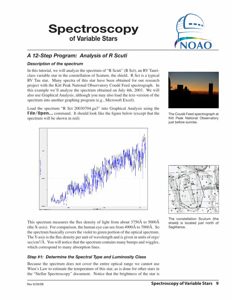
A 12-Step Program: Analysis of R ScutiDescription of the spectrum

In this tutorial, we will analyze the spectrum of “R Scuti” (R Sct), an RV Tauri-class variable star in the constellation of Scutum, the shield. R Sct is a typical RV Tau star. Many spectra of this star have been obtained for our research project with the Kitt Peak National Observatory Coudé Feed spectrograph. In this example we’ll analyze the spectrum obtained on July 4th, 2003. We will also use Graphical Analysis, although you may also load the text-version of the spectrum into another graphing program (e.g., Microsoft Excel).

Load the spectrum “R Sct 20030704.ga3” into Graphical Analysis using the File/Open... command. It should look like the figure below (except that the spectrum will be shown in red):

This spectrum measures the flux density of light from about 3750Å to 5000Å (the X-axis). For comparison, the human eye can see from 4900Å to 7000Å. So the spectrum basically covers the violet to green portion of the optical spectrum. The Y-axis is the flux density per unit of wavelength and is given in units of ergs/sec/cm2/Å. You will notice that the spectrum contains many bumps and wiggles, which correspond to many absorption lines.

Step #1: Determine the Spectral Type and Luminosity Class

Because the spectrum does not cover the entire optical range we cannot use Wien’s Law to estimate the temperature of this star, as is done for other stars in the “Stellar Spectroscopy” document. Notice that the brightness of the star is

The constellation Scutum (the shield) is located just north of Sagittarius.

The Coudé Feed spectrograph at Kitt Peak National Observatory just before sunrise.


higher at longer wavelengths. From this spectrum we cannot tell where the peak of the optical spectrum occurs, which is necessary to use Wien’s Law. We can at least tell that it is a cooler, red star.

Instead, we will use the absorption lines present in the spectrum to determine the spectral and luminosity class of the star. This is done by measuring the wavelengths of absorption lines and identifying them as described in the “Stellar Spectroscopy” document. Recall that to study the absorption lines more closely you may zoom in on portions of the spectrum and use the examine tool to measure their wavelengths. Because there are so many absorption lines in this spectrum you’ll definitely need to do this.

The Balmer series of Hydrogen lines is weak in R Sct, indicating that it is not a B, A or F star. Metal lines are not very strong in B-class stars; and in general metal lines are increasingly common in cooler stars. The strongest lines are the CaII “H&K” λλ3933,3968 lines, indicating this star is a cooler star. The lack of molecular TiO absorption bands means it is not an M-class star. It must therefore be a G or K star. Many metal lines are also present. They are too numerous to mention, however G-band λ4300 and FeII λ4175 are clearly present. Since both neutral and ionized metal lines are common in this spectrum, we conclude that this is an G-class star.

Figure 3 - Example spectra of G-class stars from figure 2v in Jacoby et al. (1984). Our spectrum covers only the portion of the spectrum blueward (left) of the vertical dashed line.

Nomenclature:

“Spectral type” is the stellar class of the star. It is based upon which absorption lines are present in a star’s spectrum, which depends primarily on the temperature of the star. The spectral classes are, from hottest to coolest, OBAFGKM. Each spectral class is divided into subclasses, indicated by an arabic number. The lower the number, the hotter the star; e.g., a B1 star is hotter than a B2.

“Luminosity class” is a refinement of the spectral type that depends on the size of the star. These classes are:

I Supergiant

II Bright Giant

III Giant

IV Subgiant

V Dwarf (“Main Sequence”)

VI Subdwarf

VII White Dwarf

Note!

The spectral class of a variable star will change over time as the star’s surface temperature changes. You will therefore need to determine the spectral class of the star for each spectroscopic observation.

The luminosity class of the star does not change, so if you deter-mine it is, e.g., a supergiant star (class Iab) from one spectroscopic observation, this will be the case for the others.

CN


To obtain a more precise spectral classification we need to compare our spectrum to the examples of G-class stars given in the Jacoby et al. (1984) library of stellar spectra. We find the best matches are with the G I (supergiant) luminosity class, as shown in Figure 3. From this figure we estimate that R Sct most closely matches spectrum #144, a G3 I class star. This is based upon the shape of the continuum and the relative strengths of several of the absorption lines. In particular, it is because of the CN molecular absorption band that appears just blueward (to the left) of the CaII absorption lines (see Figure 3). Note that you should examine other G stars in the Jacoby atlas, especially of other luminosity classes, to con-firm this estimation. Since our spectrum only covers approximately 3750Å to 5000Å, we can only compare our spectrum to the portion of the Jacoby spectral atlas blueward (left) of the dashed line in Figure 3. Also note that we may later decide to revise this classification based upon the additional information we determine about the star.

Step #2: Estimate the Star’s Effective (Surface) Temperature

Using Table 1 (below) we can estimate the effective temperature of R Sct during this particular spectroscopic observation. If the exact spectral type is not listed, you must interpolate between classes to get an estimated value. Note that you must choose a temperature from the appropriate luminosity class, e.g., from the Iab class in this case. For our G3 I classification, we must interpolate between the G2 I and G5 I values of 5200 and 4850 respectively. With a simple linear interpolation we estimate the temperature to be 5080K.

Sp. Type Iab III VT Mv T Mv T Mv

O5 40300 -6.6 42500 -6.3 44500 -5.7O6 39000 -6.5 39500 -6.1 41000 -5.5O7 35700 -6.5 37000 -5.9 38000 -5.2O8 34200 -6.5 34700 -5.8 35800 -4.9O9 32600 -6.5 32000 -5.6 33000 -4.5B0 26000 -6.4 29000 -5.1 30000 -4.0B1 20800 -6.4 24000 -4.4 25400 -3.2B2 18500 -6.4 20300 -3.9 22000 -2.4B3 16200 -6.3 17100 -3.0 18700 -1.6B5 13600 -6.2 15000 -2.2 15400 -1.2B6 13000 -6.2 14100 -1.8 14000 -0.9B7 12200 -6.2 13200 -1.5 13000 -0.6B8 11200 -6.2 12400 -1.2 11900 -0.2B9 10300 -6.2 11000 -0.6 10500 +0.2A0 9730 -6.3 10100 +0.0 9520 +0.6A1 9230 -6.4 9480 +0.2 9230 +1.0A2 9080 -6.5 9000 +0.3 8970 +1.3A3 8770 -6.5 8600 +0.5 8720 +1.5A5 8510 -6.6 8100 +0.7 8200 +1.9A7 8150 -6.6 7650 +1.1 7850 +2.2A8 7950 -6.6 7450 +1.2 7580 +2.4F0 7700 -6.6 7150 +1.5 7200 +2.7F2 7350 -6.6 6870 +1.7 6890 +3.5

Nomenclature:

The terms “early” and “late” are historical terms used to refer to spectral classes. “Early-type stars” are hotter stars, e.g., OBA stars. “Late-type stars” are cooler stars, e.g., GKM stars.

These terms should not be con-fused with similar names for galax-ies. In general, “early-type galax-ies” are elliptical galaxies. And “late-type galaxies” are spirals. Confusingly, early-type galaxies contain primarily late-type stars, and vice versa.


Sp. Type Iab III VT Mv T Mv T Mv

F5 6900 -6.6 6470 +1.6 6440 +3.6F8 6100 -6.5 6150 ––– 6200 +4.0G0 5550 -6.4 5850 +1.0 6030 +4.4G2 5200 -6.3 5450 +0.9 5860 +4.7G5 4850 -6.2 5150 +0.9 5770 +5.1G8 4600 -6.1 4900 +0.8 5570 +5.5K0 4420 -6.0 4750 +0.7 5250 +5.9K1 4330 -6.0 4600 +0.6 5080 +6.1K2 4250 -5.9 4420 +0.5 4900 +6.4K3 4080 -5.9 4200 +0.3 4730 +6.6K4 3950 -5.8 4000 +0.0 4590 +7.0K5 3850 -5.8 3950 -0.2 4350 +7.4K7 3700 -5.7 3850 -0.3 4060 +8.1M0 3650 -5.6 3800 -0.4 3850 +8.8M1 3550 -5.6 3720 -0.5 3720 +9.3M2 3450 -5.6 3620 -0.6 3580 +9.9M3 3200 -5.6 3530 -0.6 3470 +10.4M4 2980 -5.6 3430 -0.5 3370 +11.3M5 2800 -5.6 3330 -0.3 3240 +12.3M6 2600 -5.6 3240 -0.2 3050 +13.5M7 ––– ––– ––– ––– 2940 +14.3M8 ––– ––– ––– ––– 2640 +16.0

Table 1 - Temperature and absolute magnitude (Mv) for different spectral and luminosity classes. Note that these values are calculated based upon the stellar models in Schmidt-Kaler (1982).

Step #3: Determine the Julian Date of Observation

Astronomers use a decimal time system known as “Julian date.” This system makes it easier to precisely calculate how much time has elapsed between events. We need to calculate the Julian date at the time of the observation. This can be done on the AAVSO website, or on the U.S. Naval Observatory’s website:

http://aa.usno.navy.mil/data/docs/JulianDate.php


Entering the observation date of July 4th, 2003 gives a Julian date of JD 2452824.5. Note that in this case you do not need to worry about the actual time of observation. Since the star does not change noticeably in one day this is not important.

Step #4: Determine the Apparent Magnitude

Many of our stars are monitored photometrically by the Association of Amateur Variable Star Observers (AAVSO). Photometric observations are necessary because these stars change their brightness, often dramatically. For example, a portion of the long-term lightcurve for R Sct is shown below:

Note that R Sct spends most of its time around mv = +5.5. But frequently it becomes fainter by several magnitudes, over ten times fainter than normal. When determining the magnitude of R Sct it will be important to note whether R Sct is in a bright or faint state at the time of the spectroscopic observations.

The web site for the AAVSO (http://www.aavso.org) provides a light curve generator which can give (as the default) the latest time period or (what we usually need to do) a light curve covering the date of our specific spectroscopic observation of interest. Since these stars vary, it is important to get the apparent magnitude for the specific date of observation.

On the AAVSO web site, there is a box on the upper left labeled “Pick a Star”. Type the star name (R Sct in our case) into the box, select the “Create a light curve” option and click the GO button. A light curve for the past 400 days will be generated and plotted. To determine the brightness of R Sct at the time of our

Nomenclature:

Astronomers uses the magnitude scale to measure the brightness of stars. It is a logarithmic scale, wherein a change in one magni-tude corresponds to a change in brightness of 2.5 times. Note that the larger the number, the fainter the object; e.g., a magnitude 6 star is 2.5 times fainter than a magnitude 5 star.

The term “light curve” refers to a plot of the apparent magnitude (brightness) of an object over time.


spectroscopic observations, click on the link “Plot a New Light Curve.”

Set the parameters of the light curve generator to look as above. Choose start and end dates that are a month before and a month after the date of observation. Click on the “Plot Data” button to generate the light curve. A plot that looks like below should appear.

The photometric estimates are made by many different observers, leaving some uncertainty. Looking at the time of our observations (Julian date 2452824.5), the apparent magnitude is about mv = +5.5. Thus, at the time of the spectroscopic observations, R Sct was in its bright state.

Step #5: Determine the Distance via Parallax

Hipparcos was a satellite operated by the European Space Agency during 1989-1993. The primary mission of Hipparcos was to determine the distance to stars brighter than about 8th magnitude via the parallax method. A second instru-ment on Hipparcos, called TYCHO, determined parallax for fainter stars (down to about 12th magnitude) albeit with greater uncertainty. The catalogs of distance measurements from these two instruments were published in June 1997.

To determine the distance to R Sct from Hipparcos measurements we can use the SIMBAD astronomical database:

An artist’s conception of the ESA Hipparcos satellite.

Definition:

Astronomers can measure the distance to a star via the parallax method. Parallax is the apparent shift of an object’s position (relative to objects in the distance) caused by an observer changing locations. As the Earth orbits around the Sun it changes its location in space. This causes stars to shift their position, with nearby stars shifting more than distant ones.

The distance to a star can be deter-mined by measuring the angle of parallax. A star that shifts by 1 arcsecond is defined as being at a distance of 1 “parsec,” which is about 3.24 light years.


http://simbad.u-strasbg.fr/simbad/sim-fid

Enter “R Sct” into the identifier text box and click the “submit id” button. Infor-mation on this object will appear in a new window:

Don’t be confused by the different given star name. “R Sct” is just one of the many names for this star. “BD-05 4760” is another catalog’s name for this star. The Hipparcos parallax for R Sct is given as 2.32 ± 0.82 (it is shown as: 2.32 [0.82]). Note that this is in units of milli-arcseconds (mas). Remember to record the uncertainty in the parallax measurement.

To calculate the distance to R Sct is easy. The distance (in units of parsecs) is simply the inverse of the parallax:

d =1

parallax

Note that the parallax must be given in units of arcseconds. For R Sct the paral-lax is 0.00232 arcseconds, so the distance is about 431 parsecs.

Note: If a parallax for your star is not given in the Hipparcos catalog you must complete step #6. Otherwise skip ahead to step #7.

Step #6: Distance via Spectroscopic Parallax (optional)

If the parallax is unknown, we can make use of a technique known as “spectro-scopic parallax” to estimate a star’s distance. This technique uses stellar models

Warning!

Do not use the spectral type given by SIMBAD. Note that the spectral class of a variable star changes over time. The value given in SIMBAD was determined on a dif-ferent date than your observations. It is therefore likely different than what you obtained in step #1.

Nomenclature:

“Absolute magnitude” is a measure of how bright a star would appear to be if it were located 10 parsecs away from the Earth. Since a star’s apparent magnitude depends on its distance from us (by the inverse-square law), absolute magnitude is a useful means for comparing the brightness of stars that are at different distances.

Absolute magnitude is often used synonymously with luminosity for this reason because both values do not depend on the distance to the star.

Note!

Apparent magnitude is given by a lower-case “m”. And absolute magnitude is given by an upper-case “M”. To indicate in which filter the magnitude is measured, a subscript is often added; e.g., if measured through the V-band (“visible”) filter, the apparent magnitude is labeled as “mv”. If no subscript is given, assume it is measured through the V-band filter.


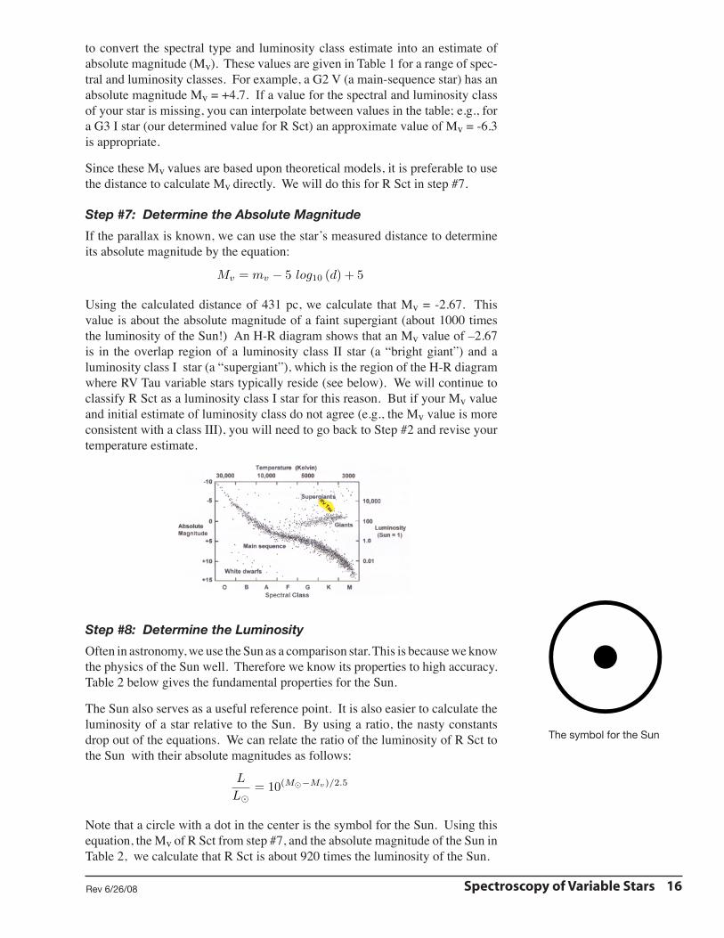
to convert the spectral type and luminosity class estimate into an estimate of absolute magnitude (Mv). These values are given in Table 1 for a range of spec-tral and luminosity classes. For example, a G2 V (a main-sequence star) has an absolute magnitude Mv = +4.7. If a value for the spectral and luminosity class of your star is missing, you can interpolate between values in the table; e.g., for a G3 I star (our determined value for R Sct) an approximate value of Mv = -6.3 is appropriate.

Since these Mv values are based upon theoretical models, it is preferable to use the distance to calculate Mv directly. We will do this for R Sct in step #7.

Step #7: Determine the Absolute Magnitude

If the parallax is known, we can use the star’s measured distance to determine its absolute magnitude by the equation:

Mv = mv − 5 log10 (d) + 5

Using the calculated distance of 431 pc, we calculate that Mv = -2.67. This value is about the absolute magnitude of a faint supergiant (about 1000 times the luminosity of the Sun!) An H-R diagram shows that an Mv value of –2.67 is in the overlap region of a luminosity class II star (a “bright giant”) and a luminosity class I star (a “supergiant”), which is the region of the H-R diagram where RV Tau variable stars typically reside (see below). We will continue to classify R Sct as a luminosity class I star for this reason. But if your Mv value and initial estimate of luminosity class do not agree (e.g., the Mv value is more consistent with a class III), you will need to go back to Step #2 and revise your temperature estimate.

Step #8: Determine the Luminosity

Often in astronomy, we use the Sun as a comparison star. This is because we know the physics of the Sun well. Therefore we know its properties to high accuracy. Table 2 below gives the fundamental properties for the Sun.

The Sun also serves as a useful reference point. It is also easier to calculate the luminosity of a star relative to the Sun. By using a ratio, the nasty constants drop out of the equations. We can relate the ratio of the luminosity of R Sct to the Sun with their absolute magnitudes as follows:

L

L�

= 10(M�−Mv)/2.5

Note that a circle with a dot in the center is the symbol for the Sun. Using this equation, the Mv of R Sct from step #7, and the absolute magnitude of the Sun in Table 2, we calculate that R Sct is about 920 times the luminosity of the Sun.

�The symbol for the Sun


Using the luminosity of the Sun from Table 2, we can now calculate that the luminosity of R Sct is 3.5 x 1036 erg/sec.

Mass (M) 1.989 x 1030 kgRadius (r) 6.96 x 108 mSurface Temperature (T) 5770 KLuminosity (L) 3.83 x 1033 erg/secAverage Density (d) 1.41 g/cm3

Spectral and Luminosity Class G2 VApparent Magnitude (mv) -26.7Absolute Magnitude (Mv) +4.74Rotational Period (equator) 25 daysAverage Sun-Earth Distance 1.496 x 1011 m (1 AU)

Table 2 - Basic astronomical data for the Sun

Step #9: Determine the Radius

The luminosity of a star depends essentially on two factors: its size and its tem-perature. Assuming a spherical star, the temperature of a star can be calculated by the equation:

L = 4πσr2T

4

Where the Stefan-Boltzmann constant is s = 5.67 x 10-8 W/m2/K4. Alternatively, its easier to calculate a star’s radius by using a ratio relative to the Sun:

L

L�

=

�

r

r�

�2 �

T

T�

�4

This causes all of the constants to cancel. Rearranging this form of the equation to solve for radius we get:

r

r�=

�

T�

T

�2

�

�

L

L�

�

Using the values for R Sct from previous steps (and from Table 2 for the Sun), we determine that the radius of R Sct is 39.1 times that of the Sun.

Using the radius of the Sun from Table 2 we calculate that this is 2.7 x 1010 m. This is about 0.18 AU (astronomical unit). So the radius of R Sct is about 18% the radius of the Earth’s orbit, or about half of the orbit of Mercury.

Step #10: Estimate the Mass

A star’s mass can be measured directly if it is in a binary star system. If this is not the case, its mass can be estimated from theoretical models based upon its spectral and luminosity classes. Table 3 below gives the estimated mass for different classes of stars. If the spectral class of your star is not present you can interpolate between classes, but note that the mass of a star changes dramatically for different classes of hot stars (the O and B stars).

Warning!

Do not confuse the mass M with absolute magnitude Mv when making calculations.


Sp. Type Iab III VO5 70 ––– 60O6 40 ––– 37O8 28 ––– 23B0 25 20 17.5B3 ––– ––– 7.6B5 20 7 5.9B8 ––– ––– 3.8A0 16 4 2.9A5 13 ––– 2.0F0 12 ––– 1.6F5 10 ––– 1.4G0 10 1.0 1.05G3 ––– ––– 1.00G5 12 1.1 0.92K0 13 1.1 0.79K5 13 1.2 0.67M0 13 1.2 0.51M2 19 1.3 0.40M5 24 ––– 0.21M8 ––– ––– 0.06

Table 3 - Masses for different spectral and luminosity classes. These values are calculated based upon the stellar models in Schmidt-Kaler (1982).

For R Sct, we estimate that its mass is about 11 times that of the Sun by inter-polating between the G0 Iab and G5 Iab classes. From Table 2, this means the mass of R Sct is about M = 2.19 x 1031 kg.

Step #11: Calculate the Density

The mean density of a star is often of use in determining its evolutionary status. The density of stars like the Sun increases towards the center, but do so in a well-understood manner. As a star evolves and moves up the H-R diagram into the giant and supergiant region, two things happen. It becomes very large in size and it becomes more dense in the core. A determination of the mean density can be used to estimate the amount of mass in the core as well as the conditions in the outer layers of the star. For some of these stars, the average density is less than the density of water, implying these stars could actually float in water (if one could find a large enough bathtub!) Assuming again that these stars are spherical, the density is calculated simply as:

d =

M

4

3πr3

For R Sct, we find a mean density of about 0.26 kg/m3. Recall that the density of water is 1000 kg/m3, so this star is on average about 4,000 times less dense than water!

Step #12: Repeat for Other Observations of R Sct

Now, step back and admire how much you have learned about this star! By fol-lowing these steps you have determined several intrinsic properties of the star.


In particular, you’ve determined its luminosity, surface temperature, distance, size, mass and average density.

But the goal of this project is to determine how these properties change over time. It is therefore necessary to repeat these steps for the other spectra obtained for this star. Because stars lose very little mass on the timescales of decades, it is safe to assume that the star’s mass and luminosity class have not changed. It is also safe to assume that the distance to the star hasn’t changed either. But surface temperature (and therefore spectral class), apparent brightness and radius very likely have changed. Thus you must repeat all of the steps (except for steps #5 or #6, and #10) for each spectroscopic observation of the star.

Once you have completed all of the steps for each available spectroscopic obser-vation of R Sct, you can create plots that show how these properties change over time. Using Graphical Analysis (or the graphing program of your choice), create plots that show how the luminosity, temperature and radius of R Sct (y-axis) change with time (x-axis). It is best (and easiest) to use the Julian date for the time. You should also generate plots of luminosity vs. temperature (i.e., an H-R diagram) as well as temperature vs. radius.

With these plots we can learn about what the star is doing as it changes. For example, we can ask these questions:

1) As the star’s luminosity increases what happens to its radius and temperature?

2) How do the star’s properties (luminosity, radius and temperature) change as it goes from its bright state to faint state?

3) Are the star’s properties random, or does it repeat in a pattern?

4) In the luminosity vs. temperature and temperature vs. radius plots, are the data points scattered randomly? Or is there a pattern? If so, what does the pattern mean?

Spectroscopy - University of Alaska systemrbseu.uaa.alaska.edu/projects/variables/Variable...

Documents

Transcript of Spectroscopy - University of Alaska systemrbseu.uaa.alaska.edu/projects/variables/Variable...