arX

iv:a

stro

-ph/

0206

225v

1 1

3 Ju

n 20

02

Spectroscopic Target Selection in the Sloan Digital Sky Survey:

The Main Galaxy Sample

Michael A. Strauss1, David H. Weinberg2,3, Robert H. Lupton1, Vijay K. Narayanan1,

James Annis4, Mariangela Bernardi5, Michael Blanton4, Scott Burles5, A. J. Connolly6,

Julianne Dalcanton7, Mamoru Doi8,9, Daniel Eisenstein5,10,20, Joshua A. Frieman4,5,

Masataka Fukugita11,3, James E. Gunn1, Zeljko Ivezic1, Stephen Kent4, Rita S.J. Kim1,12,

G. R. Knapp1, Richard G. Kron5,4, Jeffrey A. Munn13, Heidi Jo Newberg4,14, R. C. Nichol15,

Sadanori Okamura16,9, Thomas R. Quinn7, Michael W. Richmond17, David J. Schlegel1,

Kazuhiro Shimasaku16,9, Mark SubbaRao5, Alexander S. Szalay12, Dan VandenBerk4,

Michael S. Vogeley18, Brian Yanny4, Naoki Yasuda19, Donald G. York5, and Idit Zehavi4,5

1Princeton University Observatory, Princeton, NJ 08544

2Ohio State University, Dept. of Astronomy, 140 W. 18th Ave., Columbus, OH 43210

3Institute for Advanced Study, Olden Lane, Princeton, NJ 08540

4Fermi National Accelerator Laboratory, P.O. Box 500, Batavia, IL 60510

5The University of Chicago, Astronomy & Astrophysics Center, 5640 S. Ellis Ave., Chicago, IL 60637

6Department of Physics and Astronomy, University of Pittsburgh, Pittsburgh, PA 15260

7University of Washington, Department of Astronomy, Box 351580, Seattle, WA 98195

8Institute of Astronomy, School of Science, University of Tokyo, Mitaka, Tokyo, 181-0015 Japan

9Research Center for the Early Universe, School of Science, University of Tokyo, Tokyo, 181-0033 Japan

10Steward Observatory, University of Arizona, 933 N. Cherry Ave., Tucson, AZ 85721

11Institute for Cosmic Ray Research, University of Tokyo, Kashiwa, Chiba, 277-8582 Japan

12Department of Physics and Astronomy, The Johns Hopkins University, 3701 San Martin Drive, Balti-

more, MD 21218, USA

13U.S. Naval Observatory, Flagstaff Station, P.O. Box 1149, Flagstaff, AZ 86002-1149

14Physics Department, Rensselaer Polytechnic Institute, SC1C25, Troy, NY 12180

15Dept. of Physics, Carnegie Mellon University, 5000 Forbes Ave., Pittsburgh, PA-15232

16Department of Astronomy, School of Science, University of Tokyo, Tokyo, 181-0033 Japan

17Physics Department, Rochester Institute of Technology, 85 Lomb Memorial Drive, Rochester, NY 14623-

5603

18Department of Physics, Drexel University, 3141 Chestnut St., Philadelphia, PA 19104

19National Astronomical Observatory, Mitaka, Tokyo 181-8588, Japan

20Hubble Fellow

– 2 –

ABSTRACT

We describe the algorithm that selects the main sample of galaxies for spec-

troscopy in the Sloan Digital Sky Survey from the photometric data obtained

by the imaging survey. Galaxy photometric properties are measured using the

Petrosian magnitude system, which measures flux in apertures determined by the

shape of the surface brightness profile. The metric aperture used is essentially

independent of cosmological surface brightness dimming, foreground extinction,

sky brightness, and the galaxy central surface brightness. The main galaxy sam-

ple consists of galaxies with r-band Petrosian magnitude r ≤ 17.77 and r-band

Petrosian half-light surface brightness µ50 ≤ 24.5 magnitudes per square arcsec.

These cuts select about 90 galaxy targets per square degree, with a median red-

shift of 0.104. We carry out a number of tests to show that (a) our star-galaxy

separation criterion is effective at eliminating nearly all stellar contamination

while removing almost no genuine galaxies, (b) the fraction of galaxies elimi-

nated by our surface brightness cut is very small (∼ 0.1%), (c) the completeness

of the sample is high, exceeding 99%, and (d) the reproducibility of target se-

lection based on repeated imaging scans is consistent with the expected random

photometric errors. The main cause of incompleteness is blending with satu-

rated stars, which becomes more significant for brighter, larger galaxies. The

SDSS spectra are of high enough signal-to-noise ratio (S/N > 4 per pixel) that

essentially all targeted galaxies (99.9%) yield a reliable redshift (i.e., with statis-

tical error < 30 km s−1). About 6% of galaxies that satisfy the selection criteria

are not observed because they have a companion closer than the 55′′ minimum

separation of spectroscopic fibers, but these galaxies can be accounted for in

statistical analyses of clustering or galaxy properties. The uniformity and com-

pleteness of the galaxy sample make it ideal for studies of large scale structure

and the characteristics of the galaxy population in the local universe.

Subject headings: surveys — galaxies:distances and redshifts — galaxies:photometry

1. Introduction

The Sloan Digital Sky Survey (SDSS; York et al. 2000) is carrying out an imaging

survey in five photometric bands of π ster in the north Galactic cap, and a follow-up spec-

troscopic survey of roughly 106 galaxies and 105 quasars, complete within precisely defined

selection criteria. The main scientific drivers of the SDSS are the large-scale distributions

– 3 –

of galaxies and quasars. In order to carry out precise measurements of galaxy clustering

on the largest scales, and to measure the distribution of galaxy properties with the highest

possible precision, it is necessary that the sample of galaxies for which spectra are taken be

selected in a uniform and objective manner. The northern spectroscopic survey targets two

samples of galaxies: a flux-limited sample to r = 17.77 (hereafter called the main sample)

and a flux- and color-selected sample extending to r = 19.5, designed to target luminous red

galaxies (LRGs). This paper describes the algorithm used to select the main galaxy sample

and presents demonstrations that the algorithm meets the survey goals of uniformity and

completeness. A separate paper (Eisenstein et al. 2001) discusses the LRG sample.

1.1. The Sloan Digital Sky Survey

The SDSS hardware, software, and data products are summarized by York et al. (2000)

and Stoughton et al. (2002). In brief, the survey is carried out using a dedicated, wide-field

2.5m telescope, a mosaic CCD camera (Gunn et al. 1998), two fiber-fed double spectrographs,

and an auxiliary 0.5 m telescope for photometric calibration. The imaging is done in drift

scan mode with the 30 photometric CCDs of the mosaic camera imaging ≈ 20 square degrees

per hour, in five broad bands, u, g, r, i and z (Fukugita et al. 1996) that cover the entire

optical range from the atmospheric ultraviolet cutoff in the blue to the sensitivity limit of

silicon CCDs in the red. The imaging data are 95% complete for point sources at r∗ ≈ 22.2,

and the photometric calibration is accurate to about 3% in r at this writing (Hogg et al.

2001; Smith et al. 2002). Because this calibration is still preliminary, we will refer to current

measurements with the notation u∗, g∗, r∗, i∗, z∗, but we use u, g, r, i, z to refer to the

SDSS filter and magnitude system itself.21 The astrometric calibration (Pier et al. 2002) is

done by comparison with the Tycho-2 (Høg et al. 2000) and UCAC (Zacharias et al. 2000)

standards, and is accurate to 0.1 arcsec rms per coordinate.

The imaging data are reduced using a series of interlocking pipelines (photo; Lupton et

al. 2001), which flat-field the data, find all objects, match up detections in the different bands

and perform measurements of their properties, and apply the photometric and astrometric

calibrations. Spectroscopic targets — the galaxies described in this paper, LRGs (Eisenstein

et al. 2001), quasars (Richards et al. 2002), and a variety of other categories of objects

(Stoughton et al. 2002), are chosen from the resulting catalog of detected objects.

The spectroscopic component of the survey is carried out using two fiber-fed double

21This notation is a change from some earlier papers, including Fukugita et al. (1996), which referred to

the filter system as u′, g′, r′, i′, z′; see the discussion by Stoughton et al. (2002).

– 4 –

spectrographs, covering the wavelength range 3800A to 9200A over 4098 pixels. They have a

resolution λ/∆λ varying between 1850 and 2200, and together they are fed by 640 fibers, each

with an entrance diameter of 3′′. The fibers are manually plugged into plates inserted into

the focal plane; the mapping of fibers to plates is carried out by a tiling algorithm (Blanton

et al. 2001b) that optimizes observing efficiency in the presence of large-scale structure. The

finite diameter of the fiber cladding prevents fibers on any given plate from being placed

closer than 55′′ apart.

For any given plate, a series of fifteen-minute exposures is carried out until the mean

signal to noise ratio (S/N) per resolution element exceeds 4 for objects with fiber magnitudes

(i.e., as measured through the 3′′ aperture of the fiber) brighter than g∗ = 20.2 and i∗ = 19.9,

as determined by preliminary reductions done at the observing site. Under good conditions

(dark, clear skies and good seeing), this typically requires a total of 45 minutes of exposure.

1.2. The Main Galaxy Spectroscopic Sample

The main galaxy spectroscopic survey is fully sampled to its magnitude limit within

the survey footprint, which is planned to be an elliptical area of extent 110 × 130, chosen

to minimize Galactic extinction and maximize observing efficiency. The median redshift of

this sample is z ≈ 0.1. This large galaxy sample will allow us to measure many independent

modes of the density fluctuations on scales comparable to the peak of the galaxy power

spectrum, largely free from the aliasing that can affect surveys with at least one narrow

dimension (cf., Kaiser & Peacock 1991; Tegmark 1995). For some instrumental set-ups and

scientific goals (e.g., low-order measures of large scale clustering), one can gain efficiency

by sparse sampling, i.e., by observing only a fraction of the galaxies down to some limiting

magnitude (cf., Kaiser 1986). However, sparse sampling adversely affects other kinds of in-

vestigation, including group and cluster studies, high-order clustering measures, and recovery

of the underlying galaxy density field (see, e.g., Szapudi & Szalay 1996). Moreover, the field

of view and number of spectroscopic fibers of the SDSS were chosen to allow simultaneous

spectroscopy of essentially all the galaxies in a given field to the faintest magnitude for which

the 2.5m telescope can measure redshifts in a reasonable amount of time. We have therefore

opted for complete sampling in the main galaxy redshift survey.

We wish to select a magnitude-limited galaxy sample. We have carried out the selection

in a single observed band for simplicity. We wish the galaxy detection and photometric

measurement in that band to be of high S/N, and we prefer a red passband so that K

corrections are modest, fluxes are determined mainly by the older stars that dominate the

stellar mass, and uncertainties in Galactic reddening make little difference to the inferred

– 5 –

galaxy magnitude. In the SDSS filter system, this implies either the r or i band. We adopt

the former because the sky background is brighter and more variable in the i band than in

the r band. The use of a red bandpass tilts the sample slightly towards galaxies of earlier

morphological type, but at these bright magnitudes, the g − r color distribution of galaxies

is quite narrow (Ivezic et al. 2002), and the distribution of galaxy types is not radically

different from what we would obtain with g-band selection (see also Fig. 4 of Shimasaku et

al. 2001).

Although we will detail a number of subtleties below, the basic procedure that we

use to define galaxy magnitudes and select spectroscopic targets can be summarized as

follows. Star-galaxy separation is carried out by comparing the exponential or de Vaucouleurs

model magnitude of an object to its Point Spread Function (PSF) magnitude. We define

the (angular) Petrosian radius θP of a galaxy to be the radius at which the local surface

brightness in an annulus about θP is 1/5 of the mean surface brightness within θP . We

define the r-band Petrosian magnitude of a galaxy, rP , based on the flux within a circular

aperture of radius 2 θP . In the absence of seeing effects, the Petrosian magnitude measures

the light within a well-defined metric aperture on any given galaxy which is independent of

its redshift or foreground extinction. We define the half-light surface brightness µ50 to be

the mean surface brightness within a circular aperture containing half of the Petrosian flux.

The main galaxy sample consists of galaxies with rP ≤ 17.77 and µ50 ≤ 24.5 magnitudes

per square arcsec, after correcting for Galactic extinction following Schlegel, Finkbeiner, &

Davis (1998; hereafter SFD).

The outline of this paper is as follows. In § 2, we describe our goals for the target

selection algorithm. We discuss the measurements of Petrosian quantities in detail in § 3

and Appendix A. The target selection algorithm itself is described in § 4. Various tests to

show that the algorithm meets the survey requirements are described in § 5. We conclude

in § 6.

2. Desired properties of the Selection Algorithm

The SDSS spectroscopic galaxy surface density is roughly 100 galaxies per square degree.

From studies of galaxy number counts (Yasuda et al. 2001), a fully sampled magnitude-

limited survey reaches this surface density at a magnitude limit of r ≈ 18. There are several

desiderata for a galaxy spectroscopic target selection algorithm:

1. The selection algorithm should allow accurate determination of a selection function,

whereby the probability that a galaxy with given properties (magnitude, color, surface

– 6 –

brightness, redshift, position on the sky, presence of neighbors) is targeted can be

objectively quantified. To the extent possible, this selection function should depend

only on redshift, and should be independent of seeing, stellar contamination, Galactic

extinction, and spectroscopic observing conditions.

2. The algorithm should be based on physically meaningful parameters which are tied as

closely as possible to the properties of the galaxies. We must be able to measure these

parameters accurately for the sample of galaxies whose spectra we plan to obtain.

3. The algorithm should select a uniform sample of galaxies with a wide range of physical

properties, without biasing against, for example, galaxies of unusual color or low surface

brightness.

4. The algorithm should select galaxies for which we are able to obtain a spectrum of

sufficient quality to yield a redshift in the nominal exposure time. One area of concern

in this context will be galaxies with low surface brightness, for which the total light

down the 3′′ entrance aperture of the fiber will be small.

5. Finally, the selection algorithm should be simple, and its behavior should be straight-

forward and easy to understand. This makes it easier to test the algorithm, and it will

facilitate the construction of realistic mock catalogs of the SDSS galaxy redshift survey

from numerical simulations of large-scale structure (e.g., Cole et al. 1998; Colley et al.

2000).

These desiderata do not always point in the same direction. For example, one might

maximize the redshift success by selecting on the 3′′ fiber magnitude. However, this mea-

sures a fraction of the galaxy light that is strongly dependent on redshift and the atmospheric

seeing during the imaging observations, making it quite difficult to determine a meaning-

ful selection function; moreover, it biases strongly against low-surface brightness galaxies.

Similarly, isophotal magnitudes measure a fraction of the total galaxy light that depends

on foreground extinction, sky brightness (if the isophotal threshold is set relative to the sky

level), and redshift (because of cosmological surface brightness dimming). After weighing

a number of options, we have settled on an algorithm that employs a modified form of the

Petrosian (1976) magnitude system, with galaxies selected in r-band.

– 7 –

3. Petrosian Quantities

3.1. Definition of Petrosian Quantities

The Petrosian (1976) magnitude is based on the flux within an aperture defined by the

ratio of the local surface brightness to the mean interior surface brightness. The size of this

aperture depends on the shape of the galaxy’s radial surface brightness profile but not its

amplitude.

Let I(θ) be the azimuthally averaged surface brightness profile of a galaxy, as a function

of angular distance from its center, θ. We define the Petrosian ratio as the ratio of the

surface brightness in an annulus 0.8θ − 1.25θ to the mean surface brightness within θ,

R(θ) =2π

∫ 1.25θ

0.8θI(θ′)θ′dθ′/ [π((1.25θ)2 − (0.8θ)2)]

2π∫ θ

0I(θ′)θ′dθ′/(πθ2)

. (1)

The use of a fairly thick annulus reduces the sensitivity of R(θ) to noise and to small scale

fluctuations in I(θ). We define the Petrosian radius θP by the implicit equation

R(θP ) = f1 , (2)

where f1 is a constant, which we set to 0.2. The Petrosian flux is defined as the flux within

a circular aperture of radius f2 times the Petrosian radius,

FP = 2π

∫ f2θP

0

I(θ′)θ′dθ′ , (3)

and we set f2 = 2 (hereafter, we refer to f2θP as the Petrosian aperture). It will also be

useful to formally define a total flux, Ftot, as the result of the integral in equation (3) out

to infinity. The choice of f1 and f2 is discussed in §3.2 below. Note that equation (2) for

the Petrosian radius may have more than one solution; in this case, we take the outermost

of the solutions. The technical details of how photo measures all these quantities are given

in Appendix A. Note that the images of overlapping galaxies are deblended using a robust

code that conserves flux (Lupton et al., in preparation).

The Petrosian magnitude is defined from the Petrosian flux in the usual way, once the

conversion between detected counts and calibrated fluxes is determined. Note, however,

that this conversion for SDSS photometry is strictly valid only for point sources, for which

a proper aperture correction can be quantified; we ignore this complication in what follows.

Our magnitude system is based on the AB95 system (Fukugita et al. 1996); i.e., the mean flux

density over any of the broad pass-bands is f = 3631 × 10−0.4m Jy, to a fair approximation

(see the caveats in Stoughton et al. 2002). We use the asinh magnitude definition of Lupton,

– 8 –

Szalay, & Gunn (1999), which behaves well in the regime of low S/N, though for the bright

galaxies in the spectroscopic sample the difference between asinh magnitudes and traditional

logarithmic magnitudes is negligible. We refer to the r-band Petrosian apparent magnitude

as rP and to PSF and model magnitudes (see §4.2 below) as rPSF and rmodel.

Our target selection algorithm also requires a measure of surface brightness, for which

we want to retain the desirable properties of the Petrosian system. The surface brightness

within θP is an obvious choice, but it turns out to be rather noisy. Instead, we define the

Petrosian half-light radius θ50 as that which encloses half the Petrosian flux,

∫ θ50

0

I(θ′)θ′dθ′ = 0.5

∫ f2θP

0

I(θ′)θ′dθ′ , (4)

and use the mean surface brightness within this radius,

µ50 = rP + 2.5 log[

2 πθ502]

. (5)

Because the flux within 2θP is insensitive to small errors in θP , the quantities θ50 and µ50

can be robustly measured.

Figure 1 illustrates our definitions for the case of a circular de Vaucouleurs profile (top;

I(θ) = I0 exp[−7.67(θ/θe)−/4]) and a face-on exponential disk (bottom; I(θ) = I0 exp[−1.68 θ/θe]).

Dotted, dashed, and solid curves show the surface brightness profile, curve of growth, and

Petrosian ratio R(θ). Arrows mark the Petrosian half-light radius θ50, the Petrosian radius

θP at which R = f1 = 0.2 and the Petrosian aperture at f2θP = 2θP . The Petrosian radius

corresponds to 2.1 effective (or half-light) radii (3.5 scale lengths) for an exponential profile

and 1.7 effective radii for a de Vaucouleurs profile. The 2θP Petrosian aperture encompasses

99% and 82% of the galaxy’s total light in the two cases. The Petrosian half-light radius

θ50 is slightly smaller than the true half-light radius, since the Petrosian flux is less than the

total flux.

Note that we use circular apertures rather than elliptical apertures for all measurements.

Elliptical apertures are difficult to choose for galaxies whose light distributions are not well

described by concentric self-similar ellipses. Moreover, for disk galaxies, the circular-aperture

surface brightness profile is also less sensitive to inclination than the elliptical-aperture pro-

file, at least to the extent that internal extinction can be neglected. Because the Petrosian

aperture is always large enough to contain most of a galaxy’s light, the ratio of the Petrosian

flux to total flux is insensitive to inclination (or de Vaucouleurs axis ratio), as shown in

Figure 2.

In the absence of noise, the Petrosian aperture is unaffected by foreground extinction or

by the cosmological dimming of the surface brightness. Thus, identical galaxies seen at two

– 9 –

different (luminosity) distances have fluxes related exactly as distance−2 (in the absence of

K corrections). One can therefore determine the maximum distance at which a galaxy would

enter a flux-limited sample without knowing the galaxy’s surface brightness profile (which

would be needed for the equivalent calculation with, e.g., isophotal magnitudes). Moreover,

two galaxies that have the same surface brightness profile shape but different central surface

brightness have the same fraction of their flux represented in the Petrosian magnitude, so

there is no bias against the selection of low surface brightness galaxies of sufficiently bright

Petrosian magnitude. In the absence of noise, the Petrosian magnitude is independent of

sky brightness, and for the large angular extent of the galaxies of the spectroscopic sample,

it is also insensitive to seeing.

3.2. Setting f1 and f2

Here we describe the rationale behind our choice for the Petrosian parameters f1 = 0.2

and f2 = 2. Setting f1 too high would increase our sensitivity to seeing (by making θP

small), while setting it too low would require measuring the Petrosian ratio at a point that

the surface brightness is many magnitudes below that of the sky, making us particularly

sensitive to sky subtraction effects. If the Petrosian aperture f2 is too large, the measurement

of the Petrosian flux is badly affected by sky noise and uncertainty in the sky level. If the

aperture is too small, on the other hand, then the Petrosian magnitude departs substantially

from the theoretical ideal of a total magnitude, and, equally important, it becomes sensitive

to seeing and to noise in the measurement of θP .

We have carried out extensive simulations of galaxies with realistic distributions of

surface brightness and bulge-to-disk ratio (following Fukugita, Hogan, & Peebles 1998), and

have processed the resulting images through photo with a range of choices for the Petrosian

parameters. We find that seeing has an appreciable effect on the Petrosian quantities for

galaxies that would be in the spectroscopic sample, when f1 ≥ 0.25. In the simulations, only

2% of the galaxies fail to have a Petrosian radius measured (i.e., i.e., the S/N is too low

to measure the Petrosian ratio down to f1) at the spectroscopic limit for f1 = 0.2, but the

fraction of such failures becomes appreciable at smaller f1. See Yagi et al. (2002) for a similar

discussion. Note that photo still reports a reasonable measure of a “Petrosian” magnitude

even if it is unable to measure a Petrosian radius for a given object (Appendix A).

Given a value of f1, the quantity f2 sets the Petrosian aperture. Figure 3 shows the

fraction of light within the Petrosian aperture for various combinations of f1 and f2 (the

effect of seeing is not included here, but for a given value of f1, the dependence of FP /Ftot

on seeing is quite weak; see further discussion below). For many reasonable combinations of

– 10 –

Petrosian parameters, one gets almost 100% of the light in the Petrosian aperture for galaxies

with exponential profiles. De Vaucouleurs profiles are much more extended, however, and an

appreciable fraction of their light lies in the regime in which the S/N per pixel is appreciably

below unity. An aperture large enough to enclose, say, 95% of the light of a de Vaucouleurs

profile includes many low S/N pixels and thus a substantial amount of sky noise. For

f1 = 0.2, the fraction of light included in the Petrosian aperture for a de Vaucouleurs profile

rises from 82% to 89% as f2 ranges from 2 to 3. However, the simulations mentioned above

show that the photometric errors in Petrosian magnitudes at the galaxy spectroscopic survey

limit increase from 0.03 mag to 0.09 mag over this f2 range. We have therefore settled on

the value f2 = 2, to keep the S/N of Petrosian magnitudes high while still retaining most of

the light for de Vaucouleurs galaxies.

For any given morphological type (at least as defined by the surface brightness pro-

file), the correction from a Petrosian to a total magnitude is an additive constant (fixed

multiplicative factor for the flux), only weakly dependent upon inclination (Figure 2). Any

scientific analysis that uses the redshift survey must consider whether a different fraction

of light is included for ellipticals and spirals affects the result. This is important for such

analyses as the total luminosity density of the universe (e.g., Yasuda et al. 2001; Blanton et

al. 2001a), but it does not enter in calculating the radial selection function for large-scale

structure studies (as the fraction of light is independent of redshift). This dependence of

the fraction of the light measured on the galaxy light profile is unavoidable for any target

selection algorithm.

3.3. Effects of seeing, redshift, and sky background

The effect of seeing on Petrosian quantities is not completely negligible, as is shown

by Figures 1 and 2 of Blanton et al. (2001a). For a poorly resolved galaxy, the surface

brightness profile approaches that of a PSF, and the ratio of Petrosian flux to total flux

approaches 0.95, the value for a PSF. Thus, as the seeing radius approaches the half-light

radius, the Petrosian flux of an exponential galaxy is biased downward, and the Petrosian

flux of a de Vaucouleurs law galaxy is biased upward. In practice, a galaxy with θ50 = 2′′

observed in 1.5′′ seeing will have its Petrosian magnitude biased by 1-3% depending on

profile and axis ratio, and these effects are much smaller for larger galaxies (see Blanton et

al. 2001a, Fig. 1). Roughly 35% of galaxies in the spectroscopic sample have θ50 < 2′′. At

the spectroscopic magnitude limit, the typical measurement error in Petrosian magnitudes

is ∼ 0.035 magnitudes (see Figure 12 and the accompanying discussion in §5.4 below), so

seeing effects are small compared to photon noise for the great majority of galaxies in the

– 11 –

spectroscopic sample.

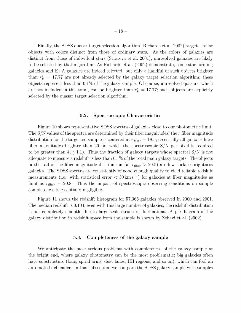
A related issue is the scaling of Petrosian magnitudes with redshift. Figure 4 shows

the redshift dependence of the measured Rp, the Petrosian radius expressed in h−1 kpc, for

galaxies in three narrow slices in absolute magnitude from the SDSS redshift survey. In the

absence of evolution and seeing effects, there should be no redshift dependence at all. In

the middle panel, the redshift dependence causes a 20% increase in the measured Petrosian

radius over the redshift range spanned; for a typical galaxy in the SDSS, the last 20% in

radius contains about 5% of the galaxy flux, which is thus an upper limit to the expected

systematic effects on redshift (Blanton et al., in preparation, conclude that the systematic

effects are in fact considerably smaller than this).

Photometry of objects requires a model for the underlying sky brightness over the extent

of the object. For objects that have at least one pixel in any band with flux greater than

200σsky, where σsky is the rms amplitude of fluctuations in sky level in that band (this

corresponds roughly to objects brighter than r∗ = 17.5), photo measures the magnitudes

twice, using two different models for the sky brightness. The first measurement (called the

BRIGHT measurement) uses a global sky value determined over an entire frame, and the

second uses a model for the local sky estimated by median-smoothing the image on a scale

of approximately 100′′, and thus will be biased high by objects of large angular extent.

The difference between these two magnitudes of an object is a reasonable estimate of the

photometric error arising from uncertainties in determining the sky underneath an object; in

particular, one might be concerned that galaxies of large angular extent will artificially raise

the estimate of the local sky, therefore biasing their photometry low. Using 210 galaxies

with r∗ < 16 from the SDSS Early Data Release (Stoughton et al. 2002), we found that

90% of the objects lie in the range −0.020 < r∗(local sky) − r∗(global sky) < 0.065. Of

course, all of these galaxies easily pass the magnitude limit, and the difference between

local and global sky subtraction is smaller for the (far more numerous) smaller galaxies with

r∗ > 16. We therefore expect negligible systematic bias in target selection associated with

sky subtraction, though there remains a small bias in the magnitudes of large galaxies much

brighter than the survey limit. For target selection, we adopt the magnitudes of all galaxies

measured using the local sky measurement.

4. The Galaxy Spectroscopic Target Selection Algorithm

The galaxy target selection algorithm is shown schematically as a flowchart in Figure 5.

The details of this algorithm have been fine-tuned largely from imaging and spectroscopic

observations of a 2.5 wide stripe, 91 degrees long, centered on the Celestial Equator in the

– 12 –

Northern Galactic Cap (Runs 752 and 756), observed during the commissioning period of

the SDSS (Stoughton et al. 2002). These are the data for which galaxy counts were pre-

sented by Yasuda et al. (2001), and the galaxy luminosity function was presented by Blanton

et al. (2001a). The distribution on the sky of galaxies selected by the algorithm is shown

in Figure 6. Large-scale structure is of course apparent. The SDSS imaging data in this

stripe are taken in a series of twelve parallel scanlines; note that the edges between scan-

lines are not apparent, which shows qualitatively that the imaging data are calibrated, and

galaxy selected, consistently. See Scranton et al. (2002) for a more detailed and quantitative

discussion of this important point.

4.1. Magnitude Limit

We select galaxy targets only from those objects that are detected in the r-band images,

i.e., which are more than 5σ above the sky after smoothing with a Point Spread Function

filter. Before the selection criteria are applied, the photometry is corrected for Galactic

extinction, using the reddening maps of SFD. The Petrosian aperture is unaffected by ex-

tinction in the absence of noise (§ 3), so the extinction correction is trivial:

rP → rP − 2.75 × E(B − V ), (6)

where the factor of 2.75 converts from the E(B−V ) reddenings reported by SFD to the r filter

shape, assuming a z = 0 elliptical galaxy spectral energy distribution. Typical extinction

values over the SDSS footprint lie in the range 0 ≤ 2.75 × E(B − V ) ≤ 0.15. There is an

effort within the SDSS collaboration to measure the reddening independently of SFD, using

the colors of halo stars, galaxy counts, and galaxy colors. This map will be used a posteriori

to derive a more accurate angular selection function, but we anticipate that errors in the

selection function associated with uncertainties in the SFD map (estimated by SFD to be

15% of the extinction itself) are already very small.

Our goal is to target a mean of 90 galaxies per square degree in the main galaxy sample.

This corresponds to a depth at which the variations of galaxy numbers due to large-scale

structure are quite substantial on degree scales, as Figure 6 shows. These fluctuations are

consistent with the measured angular correlation function of galaxies (Yasuda et al. 2001;

Scranton et al. 2002; Connolly et al. 2002). Because of these fluctuations, we need to average

over a large area of sky in order to find the magnitude limit that yields 90 galaxies per square

degree. We have carried this out over 492 square degrees of SDSS imaging data from a variety

of recent SDSS imaging runs. We have decided on a limiting magnitude of rP = 17.77, which

yields 92 galaxies per square degree in this region.

– 13 –

Although our selection boundary in apparent magnitude is formally a sharp one, in prac-

tice it is blurred (relative to that of a survey with no measurement errors) by uncertainties

in the reddening corrections and the inevitable random errors in magnitude determinations

(cf., the discussion in Appendix B). These errors need to be taken into account in statistical

analyses such as the luminosity function.

4.2. Star-galaxy Separation

Star-galaxy separation in the SDSS is described by Scranton et al. (2002). In brief,

photo generates a detailed model of the PSF at each point in each frame in each band; this

is used as a template to determine a PSF magnitude in each band, aperture-corrected to

an aperture of radius 7.4′′. In addition, each object is fit in two dimensions using a sector

fitting technique (Appendix A.1) to a de Vaucouleurs and an exponential profile of arbitrary

axis ratio and orientation, each convolved with the PSF, and aperture-corrected so that the

model and PSF magnitudes of stars (for which the model scale size will approach zero) are

equal in the mean. Each of these fits has a goodness of fit associated with it; the total

magnitude associated with the better-fit of the two models is referred to as the “model”

magnitude. A galaxy target is defined as an object for which

∆SG ≡ rPSF − rmodel ≥ 0.3 ; (7)

note that this separation is done at a somewhat more conservative cut than is done for the

star-galaxy separation in photo itself.

Figure 7 shows the distribution of Petrosian magnitude corrected for extinction as a

function of the PSF-model magnitude difference for 13772 objects brighter than r∗P = 17.8

over 115 square degrees imaged at seeing better than 1.8′′; the marginal distribution of the

magnitude difference is shown as a histogram on the bottom panel. At these relatively bright

magnitudes, the distinction between stars and galaxies is very clean, and there is no evidence

for a large population of extremely compact galaxies that could masquerade as stars. We

discuss the number of stars that masquerade as galaxies in § 5.1.

Photo models the change of the PSF on scales significantly smaller than the frame

size of 10′ × 13′. However, if the seeing changes rapidly enough, photo cannot estimate a

sufficiently accurate PSF, and the star-galaxy separation suffers. Such data are declared not

to be survey quality, and are not targeted for spectroscopic observations (see the discussion

by Stoughton et al. 2002). Any resultant holes larger than one hour in length (> 15)

are marked for reobservation. Stretches of poor data quality were not uncommon in early

SDSS commissioning data (Stoughton et al. 2002), but recent improvements to the thermal

– 14 –

environment of the survey telescope have made them increasingly rare.

4.3. Photometric Flags

As described in §3.3, objects detected at more than 200 σsky have two entries in the

database. To avoid duplicate targeting of galaxies, target selection therefore rejects one of

these two entries, that flagged as BRIGHT. The deblending procedures employed by photo are

described briefly by Stoughton et al. (2002); these procedures effectively handle star-galaxy

blends and even galaxy-galaxy blends in the great majority of cases. We only target objects

that are isolated, or children of deblends, or parents that are not deblended for one reason

or another. That is, all objects that are flagged as blended, and whose children are in the

catalog, are rejected.

The vast majority of objects that include saturated pixels are stars, even if they satisfy

the star-galaxy separation criterion of equation (7). We therefore reject all objects flagged as

SATURATED in r. We expect no more than a handful of nearby galaxies, all with bright active

nuclei, to have saturated centers in the SDSS data. However, our procedure also rejects a

small number of real galaxies that are blended with a saturated star, since the SATURATED

flag is passed onto all children of a parent with saturated pixels if the footprint of the

child includes the saturated pixels. We show in §5.3 below that the sample incompleteness

introduced by blending of galaxies with saturated stars is very small, less than 0.5%.

4.4. Surface Brightness Limits

As noted by Shectman et al. (1996) and others, every redshift survey has at least an

implicit surface brightness cut caused by detection limits of the imaging data used to derive

the input catalog, and by the limit at which the spectroscopic observations no longer yield

reliable redshifts. In order to make this cut simple and deterministic, we explicitly impose

a surface brightness cut ourselves. The distribution of objects classified as galaxies in the

magnitude-surface brightness plane is shown in Figure 8.

We target all galaxies brighter than our magnitude cut that have half-light surface

brightness µ50 ≤ 23.0 mag arcsec−2 in r; visual inspection shows that essentially all objects

down to this surface brightness limit are real galaxies. This cut already includes 99% of all

galaxies brighter than our magnitude limit. We have visually inspected about 700 lower sur-

face brightness objects in the range 23.0 ≤ µ50 ≤ 26.0 distributed over 500 square degrees of

imaging data. In the range 23.0 < µ50 < 24.5, about 65% of these galaxy target candidates

– 15 –

are in fact faint fragments of bright galaxies (usually spiral arms), cluster cores, or diffrac-

tion spikes of bright stars, erroneously pulled out by the deblending algorithm. Targeting

fragments of bright galaxies does more than waste a spectroscopic fiber; because two fibers

cannot be closer than 55′′, it can cause the nucleus of the galaxy (which will be a legitimate

galaxy target itself) not to be observed. We have found, however, that such spurious galaxy

targets have a local sky biased upwards by the parent galaxy, and we can therefore reject

them by putting a cut of 0.05 magnitudes on the difference between the local sky and the

mean global sky value measured on the frame (cf., the discussion in § 3.3). Thus, objects

in this surface brightness range are targeted only if the local and global sky values agree to

0.05 magnitudes per square arcsec. This algorithm rejects most of the contaminants while

rejecting very few genuine low surface brightness galaxies (LSBs); the fraction of remaining

objects with 23 < µ50 < 24.5 that are not real LSBs by visual inspection drops to 35%.

At surface brightnesses fainter than µ50 = 24.5, we find only 4 real LSBs (out of about

100 candidate objects) distributed over 500 square degrees, with no obvious automatic way

to distinguish them from the much more common ghost images arising due to reflections

of bright stars inside the camera. Moreover, such objects have fiber magnitudes of order

rfiber = 21 or fainter, making it unlikely that we would be able to measure a successful

redshift. We therefore do not target these objects. Low surface brightness objects tend

to be of low intrinsic luminosity, so they are visible only within a small volume, and their

rarity in the sample does not necessarily translate into a small volume density; however, they

probably contribute little to the overall luminosity density of the universe (see the discussions

by Blanton et al. 2001a; Cross et al. 2001). Since we find only four galaxies with µ50 > 24.5

in an area that contains 45,000 main sample galaxies, we estimate that only ∼ 0.01% of

galaxies brighter than our magnitude limit are rejected by our surface brightness cut.

For very nearby galaxies (cz < 10, 000 km s−1), the Petrosian half-light radius can be

quite large, substantially larger than the 3′′ aperture of the fibers. If a low-surface brightness

galaxy is strongly nucleated, our surface brightness cut can result in missing a potentially

interesting galaxy that would easily yield a redshift. We therefore accept objects of any

surface brightness brighter than our Petrosian magnitude limit, if their fiber magnitude in r

is brighter than 19.0. In practice, very few objects enter the sample this way; for example,

the stripe shown in Figure 6 contains no galaxies targeted in this manner.

There is non-negligible cross-talk between adjacent fibers in the spectrographs, thus

overly bright objects make the extraction of the spectra of neighboring faint objects difficult.

To avoid this, we reject objects whose fiber magnitude is brighter than 15 in g and r, and

14.5 in i. This criterion rejects about 0.07% of real galaxies that would otherwise be included

in the galaxy spectroscopic sample.

– 16 –

Finally, we reject all objects brighter than rP = 15.0 that have θ50 < 2′′. This cut

rejected a small number of bright stars that managed to satisfy equation (7) during the

commissioning phase of the survey, when the star-galaxy separation threshold was ∆SG =

0.15. With the final value of the cut at ∆SG = 0.3, there are no objects in Runs 752 and

756 that are rejected by this cut alone. However, we still enforce this criterion, since such

small, bright objects will saturate the spectroscopic CCDs and contaminate the spectra of

adjacent fibers, and they are in any case more likely to be star-galaxy separation errors than

actual galaxies.

4.5. Tiling and Fiber Assignment

Once targets have been selected, they are tiled, i.e., assigned to spectroscopic plates in

a way that optimizes the observing efficiency (Blanton et al. 2001b). This process leaves

essentially no systematic spatial gaps in the distribution of tiled objects, except at the outer

boundary of the tiled region (where they will be tiled in a subsequent run based on more

imaging data).

However, as mentioned earlier, fibers cannot be placed closer than 55′′, center to center,

on a given plate. The tiling algorithm maximizes the number of targeted objects given

this restriction. The tiled objects in decreasing order of priority are brown dwarfs and hot

standards (both very rare, of order one object per plate), quasar candidates (of order 100

per plate), and finally (at equal priority, and composing the bulk of the objects) the LRGs

and main sample galaxies. An object with a higher priority will never lose a fiber in favor

of a lower priority object. However, for two objects of equal priority — in particular, for

two main sample galaxies — the choice of observed target is made at random. In regions

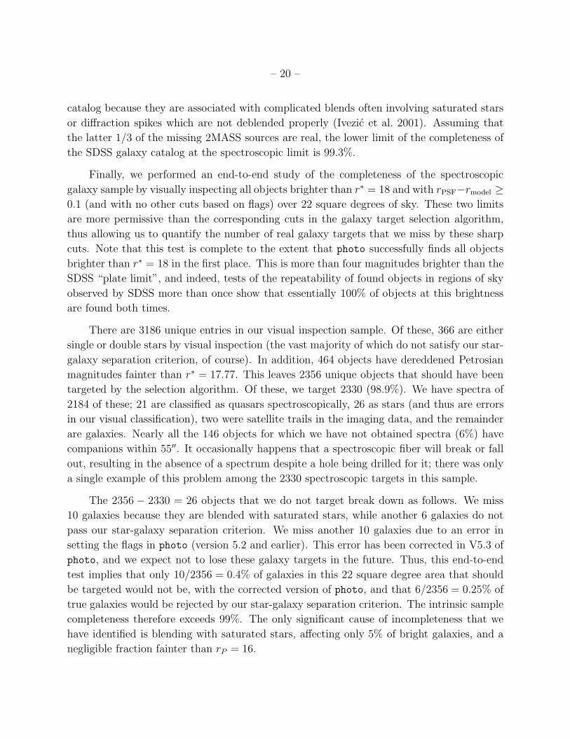
where plates overlap (roughly 30% of the tiled region), both members of a close pair are often

observed. Figure 9 shows the measured redshift difference between such pairs (Zehavi et al.

2002); 58% of close pairs have a redshift difference less than 500 km s−1 (compared with

only 4% of pairs of arbitrary angular separation). We note, however, that pairs in overlap

regions may not be representative of the full pair population, since the locations of overlap

regions are influenced by the galaxy clustering pattern.

Zehavi et al. (2002) show that for large-scale structure statistics, it is often sufficient

to simply double-weight the observed galaxy of a close pair in statistical calculations, or

to assign the unobserved galaxy the same redshift as the observed one (which is similar to

double weighting but uses the angular position of the unobserved object). Roughly 6% of

all galaxy targets are not assigned a fiber due to the 55′′ restriction.

– 17 –

5. Tests of Algorithm Performance

In this section, we present tests of the target selection algorithm. We first show (§ 5.1)

that our star-galaxy separation works well; less than 2% of the galaxy targets turn out to

be stars, while less than 0.5% of true galaxies are rejected by our algorithm. This leads

into a discussion of the spectroscopic characteristics of the sample, § 5.2. We then carry

out various tests of the completeness of the selection (§ 5.3), and find that the sample

completeness exceeds 99%, though it becomes somewhat lower for brighter galaxies, which

are more likely to be rejected because of blending with saturated stars. Finally, § 5.4 uses

repeat scans of an extended area of sky to quantify the reproducibility of the algorithm; the

differences in targeted objects are consistent with expectations due to random photometric

errors.

The SDSS science requirements for the galaxy sample include completeness of at least

95%, a redshift success rate of at least 95%, stellar contamination of less than 5%, and in-

sensitivity of selection to observing conditions during imaging. The tests below demonstrate

that the galaxy sample easily satisfies these requirements.

5.1. Tests of Star-Galaxy Separation

We select as galaxy targets objects with ∆SG ≡ rPSF − rmodel ≥ 0.3 (§ 4.2). During

the commissioning phase of the survey, we selected galaxy targets using a more permissive

value of the star-galaxy separation threshold at ∆SG = 0.15. About 3% of roughly 6000

galaxy targets selected from imaging data with seeing better than 1.8′′ lie in the range

0.15 < ∆SG < 0.6. Of these, only 10% of the targets with ∆SG < 0.3 are actually galaxies

from their spectra, while the galaxy fraction rises to 20% for those with 0.3 < ∆SG < 0.45

and to 65% for targets with 0.45 < ∆SG < 0.6. The major contaminants at lower values of

∆SG are single stars, while the contaminants above ∆SG = 0.3 are mostly double stars too

close (< 3′′) to be deblended into single stars by photo. The stellar contamination to the

galaxy sample is quite independent of seeing as long as the seeing full width at half maximum

is smaller than 1.8′′ and does not change rapidly (i.e., data of survey quality; see § 4.2).

With our final cut of ∆SG > 0.3, slightly under 2% of galaxy targets are single and

double stars. A similar fraction of the targets are classified spectroscopically as quasars;

these of course are successes of the algorithm, as they are mostly low-redshift AGN. The

spectroscopic results from the ∆SG = 0.15 threshold test run imply that only about 0.3% of

true galaxies brighter than our magnitude limit are rejected by our star-galaxy separation

criterion.

– 18 –

Finally, the SDSS quasar target selection algorithm (Richards et al. 2002) targets stellar

objects with colors distinct from those of ordinary stars. As the colors of galaxies are

distinct from those of individual stars (Strateva et al. 2001), unresolved galaxies are likely

to be selected by that algorithm. As Richards et al. (2002) demonstrate, some star-forming

galaxies and E+A galaxies are indeed selected, but only a handful of such objects brighter

than r∗P = 17.77 are not already selected by the galaxy target selection algorithm; these

objects represent less than 0.1% of the galaxy sample. Of course, unresolved quasars, which

are not included in this total, can be brighter than r∗P = 17.77; such objects are explicitly

selected by the quasar target selection algorithm.

5.2. Spectroscopic Characteristics

Figure 10 shows representative SDSS spectra of galaxies close to our photometric limit.

The S/N values of the spectra are determined by their fiber magnitudes; the r fiber magnitude

distribution for the targetted sample is centered at rfiber = 18.5; essentially all galaxies have

fiber magnitudes brighter than 20 (at which the spectroscopic S/N per pixel is required

to be greater than 4; § 1.1). Thus the fraction of galaxy targets whose spectral S/N is not

adequate to measure a redshift is less than 0.1% of the total main galaxy targets. The objects

in the tail of the fiber magnitude distribution (at rfiber > 20.5) are low surface brightness

galaxies. The SDSS spectra are consistently of good enough quality to yield reliable redshift

measurements (i.e., with statistical error < 30 km s−1) for galaxies at fiber magnitudes as

faint as rfiber = 20.8. Thus the impact of spectroscopic observing conditions on sample

completeness is essentially negligible.

Figure 11 shows the redshift histogram for 57,366 galaxies observed in 2000 and 2001.

The median redshift is 0.104; even with this large number of galaxies, the redshift distribution

is not completely smooth, due to large-scale structure fluctuations. A pie diagram of the

galaxy distribution in redshift space from the sample is shown by Zehavi et al. (2002).

5.3. Completeness of the galaxy sample

We anticipate the most serious problems with completeness of the galaxy sample at

the bright end, where galaxy photometry can be the most problematic; big galaxies often

have substructure (bars, spiral arms, dust lanes, HII regions, and so on), which can fool an

automated deblender. In this subsection, we compare the SDSS galaxy sample with samples

– 19 –

drawn from the Two Micron All-Sky Survey (2MASS)22, the Zwicky catalog, and visual

inspection of SDSS images, and show that our completeness is of order 99% overall, worsening

to 95% for galaxies brighter than r∗ = 15. Here we define completeness to be the fraction

of galaxies satisfying our selection criteria that are in fact identified as spectroscopic targets

by the automated algorithm. About 6% of these targets are not observed spectroscopically

because of the 55′′ fiber separation constraint (see §4.5). However, the locations of these

missed galaxies are known, and they can be accounted for in any statistical analysis of the

galaxy population, so we do not count them as contributing to incompleteness.

Falco et al. (1999) have compiled accurate astrometry for galaxies in the Zwicky et

al. (1961-68) catalog; we have matched this list with the SDSS database. This catalog is

limited to bZwicky = 15.7, corresponding roughly to r∗ ≈ 15. Roughly 90% of the 176 Zwicky

galaxies in 77 square degrees of sky have a corresponding SDSS main galaxy target within

3′′ of the nominal Zwicky position. Visual inspection shows that the galaxy astrometry in

the Zwicky catalog is inaccurate enough to cause a mismatch for about 5% of the galaxies;

all of these galaxies in fact have an SDSS spectroscopic galaxy target centered at the correct

photometric centroid of the galaxy. The remaining 5% of the galaxies in the Zwicky catalog

have corresponding SDSS galaxy candidates that are flagged as SATURATED due to overlap

with a saturated star (§ 4.3), and hence these galaxies will not be targeted spectroscopically.

Thus of order 95% of galaxies in the Zwicky catalog are being targeted spectroscopically. As

one goes fainter, the fraction of galaxy targets that are missed due to the SATURATED flag

will go down, since the area covered by the galaxies becomes smaller.

Yasuda et al. (2001) visually inspected all objects brighter than r∗ = 16 in the stripe

defined by Runs 752 and 756 (Stoughton et al. 2002), and classified them into stars and

galaxies. There are 1743 galaxies in this sample over 200 square degrees of sky, roughly

10% of the full galaxy sample to r∗ = 17.77 in this region. The galaxy target selection

algorithm selects 1701 (97.6%) of these bright galaxies for spectroscopic observations. Of

the 42 galaxies that are not targeted, 30 are blended with saturated stars and hence have

the SATURATED flag set, while the remaining 12 galaxies are rejected because they have fiber

magnitudes brighter than i∗ = 14.5.

Finlator et al. (2000) discuss the matching of the SDSS photometric catalog with that of

2MASS. Given typical colors of galaxies of r − K = 3.0, the SDSS spectroscopic magnitude

limit corresponds to K ≈ 14.7, which is comparable to the photometric limit of 2MASS. Of

order 2% of 2MASS point sources in the region of overlap of the two surveys are not found in

the SDSS database; of these, 2/3 are asteroids, and the remaining 1/3 do not enter the SDSS

22http://www.ipac.caltech.edu/2mass/overview/about2mass.html

– 20 –

catalog because they are associated with complicated blends often involving saturated stars

or diffraction spikes which are not deblended properly (Ivezic et al. 2001). Assuming that

the latter 1/3 of the missing 2MASS sources are real, the lower limit of the completeness of

the SDSS galaxy catalog at the spectroscopic limit is 99.3%.

Finally, we performed an end-to-end study of the completeness of the spectroscopic

galaxy sample by visually inspecting all objects brighter than r∗ = 18 and with rPSF−rmodel ≥0.1 (and with no other cuts based on flags) over 22 square degrees of sky. These two limits

are more permissive than the corresponding cuts in the galaxy target selection algorithm,

thus allowing us to quantify the number of real galaxy targets that we miss by these sharp

cuts. Note that this test is complete to the extent that photo successfully finds all objects

brighter than r∗ = 18 in the first place. This is more than four magnitudes brighter than the

SDSS “plate limit”, and indeed, tests of the repeatability of found objects in regions of sky

observed by SDSS more than once show that essentially 100% of objects at this brightness

are found both times.

There are 3186 unique entries in our visual inspection sample. Of these, 366 are either

single or double stars by visual inspection (the vast majority of which do not satisfy our star-

galaxy separation criterion, of course). In addition, 464 objects have dereddened Petrosian

magnitudes fainter than r∗ = 17.77. This leaves 2356 unique objects that should have been

targeted by the selection algorithm. Of these, we target 2330 (98.9%). We have spectra of

2184 of these; 21 are classified as quasars spectroscopically, 26 as stars (and thus are errors

in our visual classification), two were satellite trails in the imaging data, and the remainder

are galaxies. Nearly all the 146 objects for which we have not obtained spectra (6%) have

companions within 55′′. It occasionally happens that a spectroscopic fiber will break or fall

out, resulting in the absence of a spectrum despite a hole being drilled for it; there was only

a single example of this problem among the 2330 spectroscopic targets in this sample.

The 2356 − 2330 = 26 objects that we do not target break down as follows. We miss

10 galaxies because they are blended with saturated stars, while another 6 galaxies do not

pass our star-galaxy separation criterion. We miss another 10 galaxies due to an error in

setting the flags in photo (version 5.2 and earlier). This error has been corrected in V5.3 of

photo, and we expect not to lose these galaxy targets in the future. Thus, this end-to-end

test implies that only 10/2356 = 0.4% of galaxies in this 22 square degree area that should

be targeted would not be, with the corrected version of photo, and that 6/2356 = 0.25% of

true galaxies would be rejected by our star-galaxy separation criterion. The intrinsic sample

completeness therefore exceeds 99%. The only significant cause of incompleteness that we

have identified is blending with saturated stars, affecting only 5% of bright galaxies, and a

negligible fraction fainter than rP = 16.

– 21 –

Ten percent of sample galaxies have a neighbor within 55′′. The fraction of these missed

galaxies that will be recovered in a subsequent observation of an overlapping plate depends

to some extent on the size and geometry of regions that are tiled for spectroscopy, but the

estimate from this 22 square degree region that ∼ 6% of galaxy targets will ultimately remain

unobserved appears reasonable and consistent with our more recent experience.

5.4. Reproducibility

The SDSS scanlines overlap by about 1′ at their edges; moreover, we have several scans

that cover the same area of sky. This allows us to test whether we get consistent results of

photometry and main galaxy target selection in the overlaps.

We have tested the repeatability of the galaxy target selection algorithm by selecting

galaxy targets from repeated scans of the same region of the sky. In particular, the SDSS

imaging runs 745 (observed on Mar 19, 1999) and 756 (observed on Mar 21) scanned the

same patch of sky (160.5 < α < 235.5 on the Celestial equator); the six columns of the two

runs spanned the same range in declination.

Figure 12 shows the difference in the r-band Petrosian magnitudes of galaxies in common

between these runs brighter than r∗ = 18. There is no offset in the mean of the two

measurements of the Petrosian magnitudes of these galaxies, and the rms differences in the

r-band is 0.035 mag, in good agreement with the estimated Petrosian magnitude errors at

the sample magnitude limit.

Over a 90 deg2 region of repeated imaging data, we select 9159 (9125) galaxy targets from

Run 745 (756). Of these, 8652 (94.5%) targets have a corresponding target within 0.7′′ in the

other run. There are another 57 (0.6%) targets in Run 745 that have a corresponding galaxy

target within 3′′ in Run 756. Of the remaining 450 targets in Run 745 that are not selected

in Run 756, 342 objects (3.7%) have a corresponding object within 0.7′′ in Run 756 that is

fainter than the magnitude limit. This fraction is comparable to the fraction of galaxies that

is expected to cross the magnitude limit in two repeated scans because of random photometric

errors, as discussed in Appendix B. Another 78 (0.9%) targets in Run 745 are rejected by

the star-galaxy separation algorithm in Run 756, while 30 objects (0.3%) are saturated in

the Run 756 images. The discrepancy in star-galaxy separation is significantly worse than we

quoted in § 5.1, due to the fact that Run 745 had seeing significantly worse than our criterion

for survey-quality data. The fraction of targets selected from Run 756 but not from Run

745 follows similar statistics. Thus the repeatability of the galaxy target selection sample

is probably better than 95%, and nearly all of the non-repeatability can be attributed to

– 22 –

expected random photometric errors, which should not introduce any systematic biases in

statistical studies.

6. Conclusions

6.1. Summary of the algorithm performance

The main spectroscopic galaxy sample of the SDSS is a reddening-correct r-band magni-

tude limited sample of galaxies brighter than rP = 17.77, with an estimated surface density

of 92 galaxies per square degree. The magnitude is measured within a Petrosian aperture,

so as to provide a meaningful measure of a fraction of the total light of the galaxy that is

independent of distance to the galaxy, reddening, and sky background. Star-galaxy separa-

tion is based on the difference between PSF and galaxy model magnitudes, which effectively

quantifies the extension of the source relative to a PSF. We reject objects with Petrosian

half-light surface brightness µ50 > 24.5, a cut that eliminates ∼ 0.1% of galaxies brighter

than the magnitude limit. In the range 23 < µ50 < 24.5, we use a measure of the difference

between local and global sky brightness to increase our efficiency of targeting real galaxies.

We have objectively tested the star-galaxy separation algorithm and the completeness

and reproducibility of the spectroscopic sample using imaging and spectroscopic data taken

during the commissioning phase of the survey. During commissioning, we refined the criteria

in the target selection algorithm to achieve our goals on the completeness and efficiency of

the spectroscopic sample. At the time of this writing, we find that the star-galaxy separation

is accurate to better than 2%, with the main contaminants being close double stars. The

fraction of true galaxies rejected by the star-galaxy separation criterion is only ∼ 0.3%.

The completeness of the main galaxy sample is a function of magnitude. At bright

magnitudes (r∗ < 15), we find that we target 95% of the galaxies in the Zwicky catalog,

while the remaining 5% are missed because they are blended with saturated stars. From

comparison with visual inspection of bright galaxies (r∗ < 16) over 200 square degrees of

sky, we find that the completeness increases to about 97.6%. Finally, from comparison with

a visual inspection of all objects brighter than r∗ = 18 over 22 square degrees of sky, we find

that the completeness of the galaxy sample to the magnitude limit is above 99%. The only

significant source of incompleteness that we have identified is blending with saturated stars;

this incompleteness is higher for brighter galaxies because they subtend more sky.

Essentially all main sample galaxies (99.9%) that are observed spectroscopically yield

successful redshifts. About 10% of galaxy targets do not receive a fiber on the first spec-

troscopic pass because they lie within 55′′ of another sample galaxy. Some of these galaxies

– 23 –

lie in regions of plate overlap and are observed subsequently, and the fraction of galaxies

that are missed in the end because of the fiber separation constraint is about 6%. These

missing galaxies can be accounted for in any statistical analysis by appropriate weighting of

the galaxies in close pairs that are observed.

We have tested the reproducibility of the galaxy sample by selecting targets from re-

peated scans of the same region of the sky. We find that 94.5% of the spectroscopic sample

galaxies are selected in both the scans. About 3.7% of galaxies fall out of the sample because

they cross the magnitude limit and are replaced by a similar number of galaxies crossing in

the other direction; this fraction is consistent with expectations based on random errors in

the Petrosian magnitudes. Other galaxies fall out of the sample because of changes in sat-

uration or star-galaxy separation. Reproducibility of target selection is therefore high, and

the random photometric errors that lead to non-reproducibility are not expected to cause

systematic biases in statistical analyses.

6.2. Scientific applications of the SDSS imaging and spectroscopic data

The imaging data on which we tested and refined the galaxy target selection algorithm,

and the resulting galaxy spectroscopic sample have been studied in the context of both large

scale structure and properties of galaxies. Extensive tests by Scranton et al. (2001) show

that the imaging data obtained by the SDSS are free from internal and external systematic

effects that influence angular clustering for galaxies brighter than r∗ = 22, almost four

magnitudes below the limit of the spectroscopic sample. At the bright end, Yasuda et al.

(2001) studied the bright galaxy sample in the same data, and showed that the photometric

pipeline correctly identifies and deblends blended objects and provides correct photometry

for bright (r∗ < 16) galaxies.

The spectroscopic galaxy sample targeted using development versions of the target se-

lection algorithm during the commissioning phase of the survey has been used to measure

the luminosity function of galaxies as a function of surface brightness, color, and morphology

(Blanton et al. 2001). A primary goal of the SDSS is to measure the properties of large scale

structure as traced by different types of galaxies. Zehavi et al. (2002) used this spectroscopic

sample to measure the correlation function and pairwise velocity dispersion of samples de-

fined by luminosity, color, and morphology. Bernardi et al. (2002) used the spectra and

photometry to study the correlations of elliptical galaxy observables including the luminos-

ity, effective radius, surface brightness, color, and velocity dispersion. All these studies show

that the galaxies targeted spectroscopically by the SDSS constitute a uniformly selected

sample spanning a wide range of galaxy types, ideal for analyses of large scale structure and

– 24 –

galaxy properties.

Funding for the creation and distribution of the SDSS Archive has been provided by

the Alfred P. Sloan Foundation, the Participating Institutions, the National Aeronautics

and Space Administration, the National Science Foundation, the U.S. Department of En-

ergy, the Japanese Monbukagakusho, and the Max Planck Society. The SDSS Web site is

http://www.sdss.org/.

The SDSS is managed by the Astrophysical Research Consortium (ARC) for the Partic-

ipating Institutions. The Participating Institutions are The University of Chicago, Fermilab,

the Institute for Advanced Study, the Japan Participation Group, The Johns Hopkins Uni-

versity, Los Alamos National Laboratory, the Max-Planck-Institute for Astronomy (MPIA),

the Max-Planck-Institute for Astrophysics (MPA), New Mexico State University, Princeton

University, the United States Naval Observatory, and the University of Washington.

MAS acknowledges the support of NSF grants AST-9616901 and AST-0071091. DHW

acknowledges the support of NSF grant AST-0098584 and the Ambrose Monell Foundation.

A. The Calculation of Petrosian Quantities by Photo

A.1. Measuring Surface Brightnesses

The photometric pipeline, photo, measures the radial profile of every object by measur-

ing the flux in a set of annuli, spaced approximately exponentially (successive radii are larger

by approximately 1.25/0.8); the outer radii and areas are given in Table 7 of Stoughton et

al. (2002). Each annulus is divided into twelve 30 sectors. For the inner six annuli (to a

radius of about 4.6 arcsec) the flux in each sector is calculated by exact integration over the

pixel-convolved image; for larger radii the sectors are defined by a list of the pixels that fall

within their limits. Usually the straight mean of the pixel values is used, but for sectors with

more than 2048 pixels a mild clip is applied (only data from the first percentile to the point

2.3σ above the median are used).

Given a set of sectors, photo can measure the radial profile. If the mean fluxes within

each of the sectors in an annulus are Mj(j = 1, · · · , 12), it calculates a point on the profile

(‘profMean’) as

Ii =1

12

j=12∑

j=1

Mj .

The error of this quantity (‘profErr’) is a little trickier. If we knew that the object had

– 25 –

circular symmetry, we would estimate it as the variance of the Mj divided by√

12. Unfortu-

nately, in general the variation among the Mj is due both to noise and to the radial profile

and flattening of the object. To mitigate this problem, we estimate the variance as

VarI =4

9× 1

12

j=12∑

j=1

[

Mj −1

2(Mj−1 + Mj+1)

]2

, (A1)

where we interpret ‘j±1’ modulo 12, and where the factor 4/9 is strictly correct in the limit

that all the 〈Mj〉 are equal. This use of a local mean takes out linear trends in the profile

around the annulus, and results in an estimate of the uncertainty in the profile that is a

little conservative, but which includes all effects. The error due to photon noise alone, if one

needed this, could easily be calculated from the Ii and the known gain of the CCD.

In practice, photo doesn’t extract the profile beyond the point that the surface bright-

ness within an annulus falls to (or below) zero.

A.2. Measuring the Petrosian Ratio

The Ii measured in the previous subsection represent the surface brightness at some

point in the ith annulus, but exactly what point is not clear. Instead of making some

assumption about the form of the radial profile, we preferred to work with the cumulative

profile, as the Ii (and the known areas of the annuli, Ai) define unambiguous points Ci on the

object’s curve of growth. By using some smooth interpolation between these points (which,

of course, makes an assumption about the form of the radial profile) we can estimate the

surface brightness at any desired radius.

The cumulative profile has a very large dynamic range, so in practice we make this

interpolation using a cubic spline on the asinh θ vs. asinh C curve23, where θ is the angular

distance from the center of the object. As with any cubic spline, we need to specify two

additional constraints to fully determine the curve; we chose to use the ‘not-a-knot’ condition,

i.e. we force the third derivative to be continuous at the second and penultimate points. We

also used a ‘taut’ spline, which adds extra knots wherever they are needed to avoid the

extraneous inflection points characteristic of splines put through sets of points with sharp

changes of gradient (e.g., two straight line segments; de Boor 1978). We explored the use of

smoothing splines, but found that they didn’t conserve flux — it is important that the curve

actually pass through the measured points!

23We chose asinh rather than a logarithm as it is well behaved near the origin; cf. Lupton, Szalay, &

Gunn (1999).

– 26 –

The choice of boundary conditions at the origin is a little tricky. The gradient

d asinh C/d asinh θ is 0 at the origin — but only very close to the origin. For a constant

surface brightness source, once C ≫ 1, the gradient becomes very large, scaling as ≈ 1/θ

for θ ≪ 1. Experiment showed that the best results were achieved by not imposing any

symmetry (and thus gradient) constraints at θ = 0.

With the cumulative profile, expressed as a spline, in hand, the Petrosian ratio is easily

calculated, as defined in equation (1). In practice, we evaluate R at the annular boundaries θi

(where we know the cumulative profile), and use another taut not-a-knot spline to interpolate

R as a function of asinh θ.

We estimate the uncertainty σR in R by propagating errors in equation (1) on the

assumption of Poisson noise in the object and sky; we allow for the covariance between the

numerator and denominator and only work to quadratic order in the errors. However, if

the resulting S/N exceeds that of the measured radial profile at that point (measured as

described in eq. A1), the error in R is set to R times the error in the radial profile.

A.3. Measuring the Petrosian Flux

The Petrosian radius θP is found by solving the equation R(θP ) = f1. We’ve expressed

R as a cubic spline, so we can piecewise apply the usual analytic formula for the roots of a

cubic and find all Petrosian radii (there may indeed be more than one solution; see below).

Clearly R(0) = 1, and for most forms of an object’s radial profile R(∞) = 0 (the exception

being a power law P (θ) ∝ θ−α, with R(∞) = (α − 2)/α), so almost all objects will have at

least one θP .

Even in the absence of noise, some objects may have more than one θP ; the Petrosian

ratio need not be monotonic in θ. For example, a galaxy with an AGN can have one Petrosian

radius for the part of the galaxy where its light is dominated by the nucleus and another,

larger, θP associated with the extended light; in this case we should adopt the larger value.

On the other hand, a bright star with a much fainter galaxy nearby that has not been

properly deblended can have a small θP associated with the star, and another much larger

value produced by a small rise in the radial profile at the position of the galaxy, at a radius

where the mean enclosed surface brightness due to the star has fallen to a low value; in this

case we should adopt the smaller value.

These spurious values of θP are found at a point where the surface brightness is very

low, so we have adopted the following procedure, setting flags for each object to describe

any unusual problems we come across, as described by Stoughton et al. (2002):

– 27 –

• Find all of the object’s Petrosian radii, as described above.

• If there is no Petrosian radius, R must be above f1 at the last measured point in the

profile (remember that θP (0) ≡ 1). We thus take θP to be the outermost measured

point in the profile (this is equivalent to assuming that the surface brightness is exactly

zero beyond this point). We then set the NOPETRO and NOPETRO BIG flags and proceed

to measuring other quantities.

• Otherwise, reject all the values of θP where the corresponding surface brightness (as

estimated by differentiating the spline representation of the cumulative surface bright-

ness) is below µmin = 25 mag arcsec−2. If any values are rejected, we set the PETROFAINT

flag.

• Keep the largest surviving θP . If there is more than one, set the MANYPETRO flag.

• If there are no surviving radii, set the NOPETRO flag; set θP = θP min = 3′′.

Once we know θP , we can estimate its error σθP. We find the Petrosian radii (following

the above prescription) corresponding to Petrosian ratios R + σR and R − σR. Half the

difference between them is the estimated error on θP . This simple approach ignores covari-

ances between the estimates, but gives correct errors within 20% as determined from repeat

measurements.

The Petrosian flux FP is defined as the flux within f2 × θP ; in all bands the θP used is

that measured in the r band. If f2 × θP exceeds the last measured point on the profile, the

total flux to that point is used (once again, this corresponds to assuming that the surface

brightness falls to zero at this point, as this is the only reasonable assumption we could

make). This happens for only 2% of galaxies brighter than the spectroscopic limit. The

error in the Petrosian flux σFPis made up of two terms, added in quadrature: The photon

noise within f2θP due to the object and sky, and a term due to the uncertainty in θP . This

second term is 0.5 [C(θP + σθP) − C(θP − σθP

)], where C is the cumulative profile as above.

We neglect the covariance between these two terms; the contribution to the photon noise

from the region between θP + σθPand θP − σθP

is negligible; the uncertainty in θP is also

mostly determined locally, and is thus more-or-less uncorrelated with the Poisson term. Both

terms are included in all bands, even though the Petrosian aperture is based on the r band

Petrosian radius for all bands. § 5.4 showed that the resulting errors are quite accurate.

We also calculate two concentration parameters θ50 and θ90, the radii containing 50%

and 90% of the Petrosian flux. Their errors are naıvely estimated as e.g. 0.5(θ50,FP +σFP−

θ50,FP−σFP) where θ50,FP +σFP

is the value of θ50 that we’d estimate if the Petrosian flux were

– 28 –

FP + σFP. Repeat measurements show that the errors in θ50 are overestimated by a factor

of two at r∗ = 18, while the errors in θ90 are correct to 10%.

B. On the fraction of galaxy targets crossing the magnitude limits in repeated

scans

The Petrosian magnitudes have finite errors, and thus a sharp cut in observed magnitude

will be a slightly fuzzy cut in true magnitudes. One effect, as we saw in § 5.4, is that samples

defined from repeat imaging scans of the same area of sky will not be identical. We quantify

the expected effect here.

The probability that a galaxy with a true magnitude m is observed to be brighter than

the magnitude limit ml in one scan and fainter than the magnitude limit in another scan is

given by

P (m) = p(m) [1 − p(m)] , (B1)

where

p(m) =1√

2πσm

∫ ml

−∞

e−

(m−ml)

2

2σ2m dml ≡

1

2erfc

(

m − ml√2σm

)

(B2)

is the probability that a galaxy is brighter than the magnitude limit in one scan, and σm

is the error in photometry (in magnitudes), which we assume is distributed as a Gaussian.

Hence, the fraction of galaxy targets that are targeted in one scan but not in the other is

F (m1 < ml, m2 > ml) =

∫

∞

−∞n(m)p(m) [1 − p(m)]∫

∞

−∞n(m)p(m)

, (B3)

where n(m) is the differential number counts of galaxies as a function of magnitude.

Yasuda et al. (2001) have found that n(m) ∝ 100.55m near the magnitude limit of

ml = 17.77 in the r-band. At this magnitude, σm = 0.035 mag, and equation (B3) predicts

that about 3.2% of galaxies to cross the magnitude limit in two repeated scans, due to

random photometric errors alone. This predicted fraction is very close to the fraction 3.7%

found in the test discussed in §5.4.

REFERENCES

Bernardi, M. et al. 2002, AJ, in press (astro-ph/0110344)

Blanton, M. et al. 2001a, AJ, 121, 2358

– 29 –

Blanton, M. et al. 2001b, AJ, submitted (astro-ph/0105535)

Cole, S., Hatton, S., Weinberg, D.H., & Frenk, C.S., 1998, MNRAS, 300, 945

Colley, W. N., Gott, J. R., Weinberg, D. H., Park, C., & Berlind, A. A. 2000, ApJ, 529, 795

Connolly, A. et al. 2002, ApJ, in press (astro-ph/0107417)

Cross, N. et al. 2001, MNRAS, 324, 825

de Boor, C. 1978, A Practical Guide to Splines (N.Y.: Springer-Verlag)

Eisenstein, D. et al. 2001, AJ, 122, 2267

Falco, E.E. et al. 1999, PASP, 111, 438

Finlator, K. et al. 2000, AJ, 120, 2615

Fukugita, M., Hogan, C. J. & Peebles, P. J. E. 1998, ApJ, 503, 518

Fukugita, M. Ichikawa, T. Gunn, J. E., Doi, M., Shimasaku, K. & Schneider, D. P. 1996,

AJ, 111, 1748

Gunn, J.E. et al. 1998, AJ, 116, 3040

Høg, E., Fabricius, C., Makarov, V. V., Urban, S., Corbin, T., Wycoff, G., Bastian, U.

Schwekendiek, P., & Wicenec, A. 2000, A&A, 355, L27

Hogg, D.W., Schlegel, D.J., Finkbeiner, D.P., & Gunn, J.E. 2001, AJ, 122, 2129

Ivezic, Z. et al. 2001, AJ, 122, 2749

Ivezic, Z. et al. 2002, AJ, submitted (astro-ph/0202408)

Kaiser, N. 1986, MNRAS, 219, 785

Kaiser, N., & Peacock, J.A. 1991, ApJ, 379, 482

Lupton, R.H., Szalay, A.S., & Gunn, J.E. 1999, AJ, 118, 1406

Lupton, R., Gunn, J. E., Ivezic, Z., Knapp, G. R., Kent, S., & Yasuda, N. 2001, in ASP Conf.

Ser. 238, Astronomical Data Analysis Software and Systems X, ed. F. R. Harnden,

Jr., F. A. Primini, and H. E. Payne (San Francisco: Astr. Soc. Pac.), 269

Petrosian, V. 1976, ApJ, 209, L1

– 30 –

Pier, J.R., Munn, J.A., Hindsley, R.B., Hennessy, G.S., Kent, S.M., Lupton, R.H., & Ivezic,

Z. 2002, AJ, submitted

Richards, G. et al. 2002, AJ, 123, 2945

Schlegel, D., Finkbeiner, D., & Davis, M. 1998, ApJ, 500, 525

Scranton, R. et al. 2002, ApJ, in press (astro-ph/0107416)

Shectman, S. et al. 1996, ApJ, 470, 172

Shimasaku, K. et al. 2001, AJ, 122, 1238

Smith, J.A. et al. 2002, AJ, 123, 2121

Stoughton, C. et al. 2002, AJ, 123, 485

Strateva, I. et al. 2001, AJ, 122, 1861

Szapudi, I., & Szalay, A. 1996, ApJ, 459, 504

Tegmark, M. 1995, ApJ, 455, 429

Yagi, M., Kashikawa, N., Sekiguchi, M., Doi, M., Yasuda, N., Shimasaku, K., & Okamura,

S. 2002, AJ, 123, 66

Yasuda, N. et al. 2001, AJ, 122, 1104

York, D.G. et al. 2000, AJ, 120, 1579

Zacharias, N., Urban, S. E., Zacharias, M. I., et al. 2000, AJ, 120, 2131

Zehavi, I. et al. 2002, ApJ, 571, 172

Zwicky, F., Herzog, E., Wild, P., Karpowicz, M., & Kowal, C. 1961-68, Catalogue of Galaxies

and of Clusters of Galaxies, (Pasadena: California Institute of Technology)

This preprint was prepared with the AAS LATEX macros v5.0.

– 31 –

Fig. 1.— Illustration of the Petrosian aperture procedure for a de Vaucouleurs profile (top)

and an exponential profile (bottom), assuming an axis ratio of one and negligible seeing.

In each panel, the dashed curve shows the curve of growth (fraction of total light within

radius θ), and the solid curve shows the Petrosian ratio R(θ). The dotted curve shows the

logarithmic surface brightness profile, using the right-hand axis scale. The central arrow

marks the Petrosian radius at R(θ) = 0.2. Outer and inner arrows represent the radius of

the Petrosian aperture (f2θP ) and the Petrosian half-light radius θ50, respectively. All radii

are scaled to the true half-light radius θe, which is 1.678 scale lengths for the exponential

profile.

– 32 –

Fig. 2.— Effect of axis ratio on the Petrosian flux, measured using our circular aperture

definitions of Petrosian quantities. The dashed line shows the fraction of the total flux within

the Petrosian aperture for inclined exponential disks as a function of axis ratio. The solid

line shows the same quantity for a de Vaucouleurs law galaxy. The dotted line represents

a galaxy with an inclined (exponential) disk and a circular (de Vaucouleurs law) bulge,

assuming a 1:1 bulge-to-disk ratio and a bulge half-light radius that is half that of the disk.

– 33 –

Fig. 3.— The fraction of the total light within the Petrosian aperture f2θP as a function of

the value of f2, for f1 = 1/5 (solid lines), 1/6 (dotted lines), and 1/4 (dashed lines). Lower

curves correspond to de Vaucouleurs law profiles and upper curves to exponential profiles.

Filled circles mark our adopted values f1 = 1/5, f2 = 2. These calculations simulate idealized

circular galaxies, and seeing is assumed to be negligible.

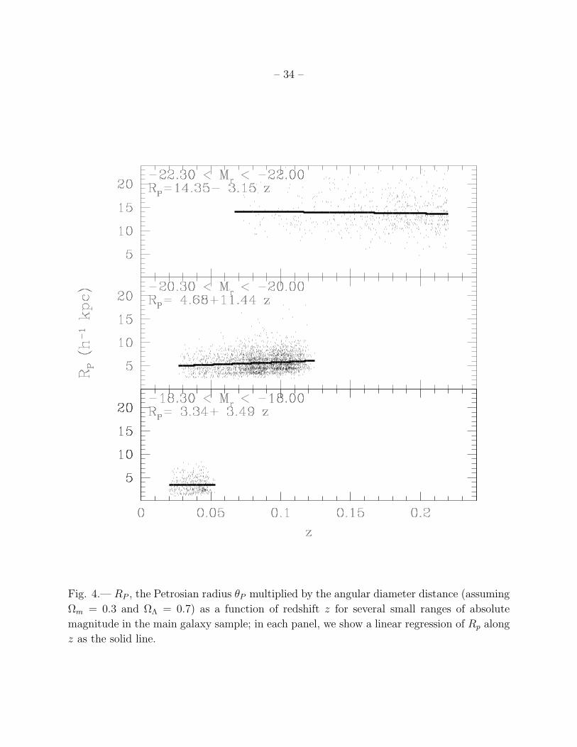
– 34 –

Fig. 4.— RP , the Petrosian radius θP multiplied by the angular diameter distance (assuming

Ωm = 0.3 and ΩΛ = 0.7) as a function of redshift z for several small ranges of absolute

magnitude in the main galaxy sample; in each panel, we show a linear regression of Rp along

z as the solid line.

– 35 –

> 5 in r? -No Reject?YesStar/gal separation: rPSF rmodel 0:3? -No Reject?YesSATURATED, BRIGHT, or BLENDED? -Yes Reject?NorP 17:77? -No RejectYes? ? ?50 23:0? 23:0 < 50 24:5? 50 > 24:5??AcceptYes ?Skyglobal Skylocal < 0:05or rber 19:0??AcceptYes

?rber 19:0??AcceptYes

Fig. 5.— Schematic flow diagram of the main galaxy target selection algorithm. All quan-

tities are measured in the r band and are corrected for foreground extinction. See the text

for a full description of all quantities referred to in this figure.

– 36 –

Fig. 6.— The distribution of objects on the sky targeted by the galaxy target selection

algorithm, in a stripe 2.5 wide centered on the Celestial Equator. We have spectra of

essentially all these objects. The stripe is 91 degrees long, 145 < α(2000) < 236, and is

broken into contiguous pieces for the figure.

– 37 –

Fig. 7.— The relationship between Petrosian magnitude corrected for Galactic extinction,

and the difference between PSF and model magnitude in the r band, for stars and galaxies

in 115 square degrees. The separation between stars and galaxies is apparent with a simple

cut in the difference between PSF and model magnitude. The distribution of this difference

for objects brighter than r∗ = 17.8 is shown in the lower panel.

– 38 –

Fig. 8.— The distribution of objects classified as galaxies with r∗P ≤ 17.77 in the de-reddened,

r-band, Petrosian magnitude-Petrosian surface brightness plane. The cuts at µ50 = 23.0 and

24.5 are indicated. The lower panel shows the differential (histogram; left-hand axis) and

cumulative (dotted curve; right-hand axis) distribution of surface brightness; of order 1% of

galaxies brighter than the magnitude limit have µ50 > 23.0.

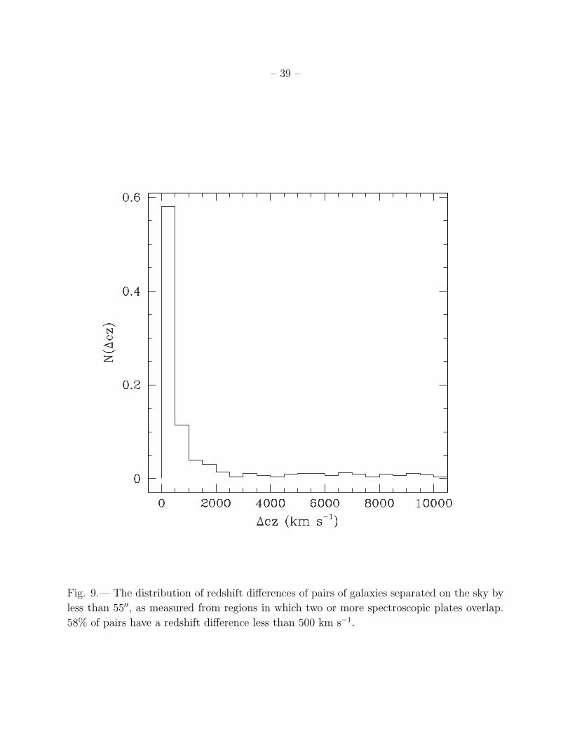
– 39 –

Fig. 9.— The distribution of redshift differences of pairs of galaxies separated on the sky by

less than 55′′, as measured from regions in which two or more spectroscopic plates overlap.

58% of pairs have a redshift difference less than 500 km s−1.

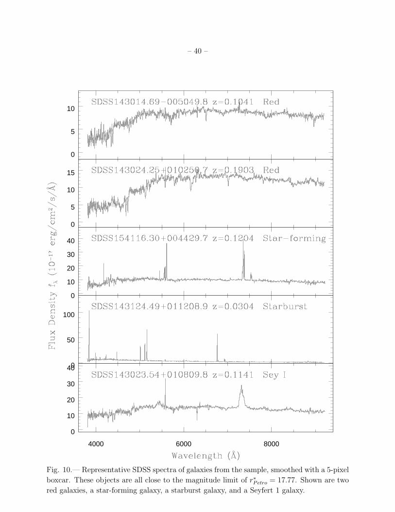
– 40 –

0

5

10

0

5

10

15

0

10

20

30

40

0

50

100

4000 6000 8000

0

10

20

30

40

Fig. 10.— Representative SDSS spectra of galaxies from the sample, smoothed with a 5-pixel

boxcar. These objects are all close to the magnitude limit of r∗Petro = 17.77. Shown are two

red galaxies, a star-forming galaxy, a starburst galaxy, and a Seyfert 1 galaxy.

– 41 –

Fig. 11.— The redshift histogram of 57,366 galaxies selected by the algorithm; the y-axis is

the number of galaxies in bins of 0.01 in redshift. Even this large number of galaxies is not

quite enough to average over large-scale structure fluctuations.

– 42 –

Fig. 12.— The difference between the r-band Petrosian magnitudes of the same galaxies

measured in two different imaging runs. The dashed line shows the magnitude limit rP =

17.77 of the main galaxy sample.