Spectral Methods for Ranking and Constrained...
91
1 Spectral Methods for Ranking and Constrained Clustering Mihai Cucuringu University of Oxford Alan Turing Institute April 14, 2017
Transcript of Spectral Methods for Ranking and Constrained...

1
Spectral Methods for Ranking andConstrained Clustering
Mihai Cucuringu
University of OxfordAlan Turing Institute
April 14, 2017
2
Outline
I Synchronization RankingI M. Cucuringu, Sync-Rank: Robust Ranking, Constrained
Ranking and Rank Aggregation via Eigenvector and SDPSynchronization, IEEE Transactions on Network Scienceand Engineering (2016)
I Constrained clusteringI M. C., I. Koutis, S. Chawla, G. Miller, and R. Peng, Simple
and Scalable Constrained Clustering: A GeneralizedSpectral Method , AISTATS 2016
3
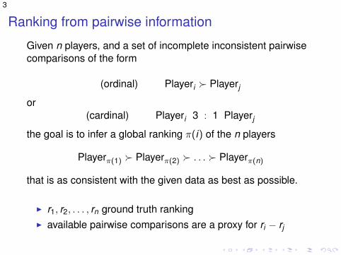
Ranking from pairwise information
Given n players, and a set of incomplete inconsistent pairwisecomparisons of the form
(ordinal) Playeri � Playerj
or(cardinal) Playeri 3 : 1 Playerj
the goal is to infer a global ranking π(i) of the n players
Playerπ(1) � Playerπ(2) � . . . � Playerπ(n)
that is as consistent with the given data as best as possible.
I r1, r2, . . . , rn ground truth rankingI available pairwise comparisons are a proxy for ri − rj

4
Roadmap
I Related methodsI Serial-RankI Rank-CentralityI SVD-based rankingI Ranking via least-squares
I The group synchronization problemI Ranking via angular synchronizationI Numerical experiments on synthetic and real dataI Rank aggregation; Ranking with hard constraints

5
Challenges
I in most practical applications, the available informationI is usually incomplete, especially when n is largeI is very noisy, most measurements are inconsistent with the
existence of an underlying total orderingI at sports tournaments (G = Kn) the outcomes always
contain cycles: A beats B, B beats C, and C beats AI aim to recover a total (or partial) ordering that is as
consistent as possible with the dataI minimize the number of upsets: pairs of players for which
the higher ranked player is beaten by the lower ranked one
6
Applications
Instances of such problems are abundant in various disciplines,especially in modern internet-related applications such as
I the famous search engine provided by GoogleI eBay’s feedback-based reputation mechanismI Amazon’s Mechanical Turk (MTurk) crowdsourcing system
enables businesses to coordinate the use of human laborto perform various tasks
I Netflix movie recommendation systemI Cite-Seer network of citationsI ranking of college football/basketball teamsI ranking of math courses for students based on grades
7
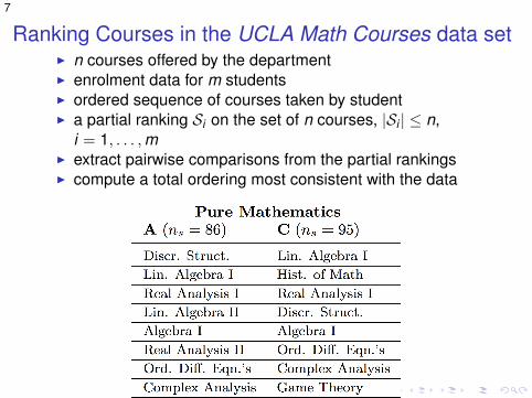
Ranking Courses in the UCLA Math Courses data setI n courses offered by the departmentI enrolment data for m studentsI ordered sequence of courses taken by studentI a partial ranking Si on the set of n courses, |Si | ≤ n,
i = 1, . . . ,mI extract pairwise comparisons from the partial rankingsI compute a total ordering most consistent with the data
Figure: Comparing the A and C students in the Pure Math majorsusing SyncRank.
8
Very rich literature on ranking
I dates back as early as the 1940s (Kendall and Smith)I PageRank: used by Google to rank web pages in
increasing order of their relevanceI Kleinberg’s HITS algorithm: another website ranking
algorithm based on identifying good authorities and hubsfor a given topic queried by the user
Traditional ranking methods fall short:I developed with ordinal comparisons in mind (movie X is
better than movie Y )I much of the current data deals with cardinal/numerical
scores for the pairwise comparisons (e.g., goal differencein sports)
9
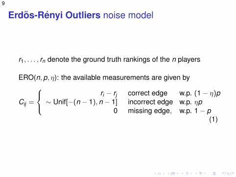
Erdos-Renyi Outliers noise model
r1, . . . , rn denote the ground truth rankings of the n players
ERO(n,p, η): the available measurements are given by
Cij =
ri − rj correct edge w.p. (1− η)p
∼ Unif[−(n − 1),n − 1] incorrect edge w.p. ηp0 missing edge, w.p. 1− p
(1)
10
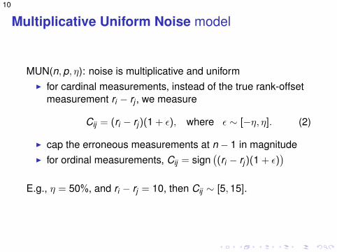
Multiplicative Uniform Noise model
MUN(n,p, η): noise is multiplicative and uniformI for cardinal measurements, instead of the true rank-offset
measurement ri − rj , we measure
Cij = (ri − rj)(1 + ε), where ε ∼ [−η, η]. (2)
I cap the erroneous measurements at n − 1 in magnitudeI for ordinal measurements, Cij = sign
((ri − rj)(1 + ε)
)E.g., η = 50%, and ri − rj = 10, then Cij ∼ [5,15].
11
Serial-Ranking (NIPS 2014)
I Fogel et al. adapt the seriation problem to rankingI propose an efficient polynomial-time algorithm with
provable recovery and robustness guaranteesI perfectly recovers the underlying true ranking, even when a
fraction of the comparisons are either corrupted by noiseor completely missing
I more robust to noise that other classical scoring-basedmethods from the literature
12
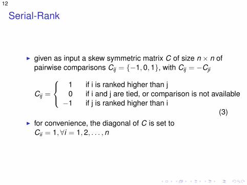
Serial-Rank
I given as input a skew symmetric matrix C of size n × n ofpairwise comparisons Cij = {−1,0,1}, with Cij = −Cji
Cij =
1 if i is ranked higher than j0 if i and j are tied, or comparison is not available−1 if j is ranked higher than i
(3)I for convenience, the diagonal of C is set to
Cii = 1,∀i = 1,2, . . . ,n
13
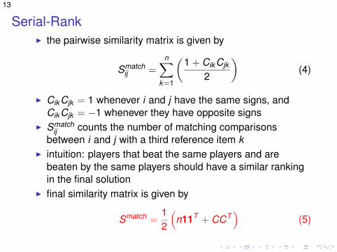
Serial-RankI the pairwise similarity matrix is given by
Smatchij =
n∑k=1
(1 + CikCjk
2
)(4)
I CikCjk = 1 whenever i and j have the same signs, andCikCjk = −1 whenever they have opposite signs
I Smatchij counts the number of matching comparisons
between i and j with a third reference item kI intuition: players that beat the same players and are
beaten by the same players should have a similar rankingin the final solution
I final similarity matrix is given by
Smatch =12
(n11T + CCT
)(5)

14
Figure: Smatch similarity
Clean Rank-Offset:
5 10 15 20
2
4
6
8
10
12
14
16
18
20
−15
−10
−5
0
5
10
15

15Algorithm 1 Serial-Rank: an algorithm for spectral ranking us-ing seriation, proposed by Fogel, d’Aspremont and VojnovicRequire: A set of pairwise comparisons Cij ∈ {−1,0,1} or [-
1,1]1: Compute a similarity matrix as shown in (4)2: Compute the associated graph Laplacian matrix
LS = D − S (6)
where D is a diagonal matrix D = diag (S1), i.e., Dii =∑nj=1 Si,j is the degree of node i .
3: Compute the Fiedler vector of S (eigenvector correspondingto the smallest nonzero eigenvalue of LS).
4: Output the ranking induced by sorting the Fiedler vector ofS, with the global ordering (increasing or decreasing order)chosen such that the number of upsets is minimized.
15
Rank Centrality (NIPS 2012)
I Negahban, Oh, Shah, ”Rank Centrality: Ranking fromPair-wise Comparisons”, NIPS 2012
I algorithm for rank aggregation by estimating scores for theitems from the stationary distribution of a certain randomwalk on the graph of items
I edges encode the outcome of pairwise comparisonsI proposed for the rank aggregation problem: a collection of
sets of pairwise comparisons over n players, given by kdifferent ranking systems

16
Rank Centrality; k > 1 rating systemsI the BTL model assumes that
P(Y (l)ij = 1) =
wj
wi + wj
I w is the vector of positive weights associated to the players
I RC starts by estimating the fraction of times j defeated i
aij =1k
k∑l=1
Y (l)ij
I consider the symmetric matrix
Aij =aij
aij + aji(7)
Pij =
{1
dmaxAij if i 6= j
1− 1dmax
∑k 6=i Aik if i = j ,
(8)
where dmax denotes the maximum out-degree of a node.
17
Singular Value Decomposition (SVD) rankingI for cardinal measurements, the noiseless matrix of rank
offsets C = (Cij)1≤i,j≤n is a skew-symmetric of even rank 2
C = reT − erT (9)
where e denotes the all-ones column vector.I {v1, v2,−v1,−v2}: order their entries, infer rankings, and
choose whichever minimizes the number of upsetsI ERO noise model
ECij = (ri − rj)(1− η)p, (10)
I EC is a rank-2 skew-symmetric matrix
EC = (1− η)p(reT − erT ) (11)
I decompose the given data matrix C as
C = EC + R (12)

18
Ranking via Least-Squares
I m = |E(G)|I denote by B the edge-vertex incidence matrix of size m× n
Bij =
1 if (i , j) ∈ E(G), and i > j−1 if (i , j) ∈ E(G), and i < j
0 if (i , j) /∈ E(G)(13)
I w the vector of size m × 1 containing all pairwisecomparisons w(e) = Cij , for all edges e = (i , j) ∈ E(G).
I least-squares solution to the ranking problem
minimizex∈Rn
||Bx − w ||22. (14)

19
Synchronization over SO(2)
Estimate n unknown angles
θ1, . . . , θn ∈ [0,2π),
given m noisy measurements Θij of their offsets
Θij = θi − θj mod 2π. (15)
Challenges:I amount of noise in the offset measurementsI only a very small subset of all possible pairwise offsets are
measured

20
Synchronization over Z2
3
2
1
4
5
6
+1
+1
+1 -‐1
-‐1
-‐1
+1 +1
+1 +1 -‐1 -‐1 -‐1
-‐1 -‐1
-‐1
3
2
1
4
5
6
+1
+1
+1 -‐1
-‐1
-‐1
-‐1 +1
+1 +1 1 -‐1 1
-‐1 -‐1
1
Figure: Synchronization over Z2 (left: clean, right: noisy)
Zij =
ziz−1
j (i , j) ∈ E and the measurement is correct,−ziz−1
j (i , j) ∈ E and the measurement is incorrect,0 (i , j) /∈ E
I original solution: z1, . . . , zNI approximated solution: x1, . . . , xNI task: estimate x1, . . . , xN such that we satisfy as many
pairwise group relations in Z as possible
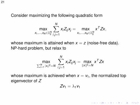
21
Consider maximizing the following quadratic form
maxx1,...,xN∈ZN
2
N∑i,j=1
xiZijxj = maxx1,...,xN∈ZN
2
xT Zx ,
whose maximum is attained when x = z (noise-free data).NP-hard problem, but relax to
max∑Ni=1 |xi |2=N
N∑i,j=1
xiZijxj = max‖x‖2=N
xT Zx
whose maximum is achieved when x = v1, the normalized topeigenvector of Z
Zv1 = λ1v1
22
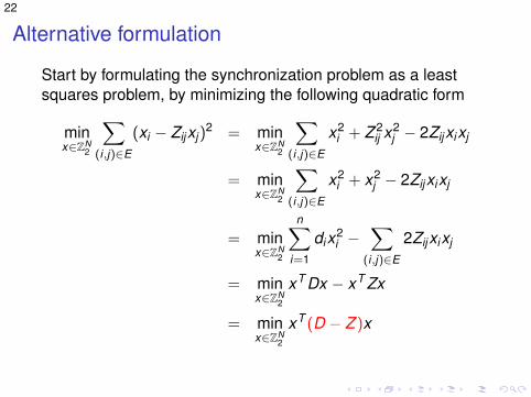
Alternative formulation
Start by formulating the synchronization problem as a leastsquares problem, by minimizing the following quadratic form
minx∈ZN
2
∑(i,j)∈E
(xi − Zijxj)2 = min
x∈ZN2
∑(i,j)∈E
x2i + Z 2
ij x2j − 2Zijxixj
= minx∈ZN
2
∑(i,j)∈E
x2i + x2
j − 2Zijxixj
= minx∈ZN
2
n∑i=1
dix2i −
∑(i,j)∈E
2Zijxixj
= minx∈ZN
2
xT Dx − xT Zx
= minx∈ZN
2
xT (D − Z )x
23
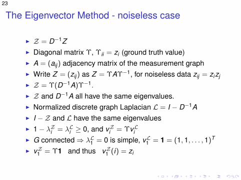
The Eigenvector Method - noiseless case
I Z = D−1ZI Diagonal matrix Υ, Υii = zi (ground truth value)I A = (aij) adjacency matrix of the measurement graphI Write Z = (zij) as Z = ΥAΥ−1, for noiseless data zij = zizj
I Z = Υ(D−1A)Υ−1.
I Z and D−1A all have the same eigenvalues.I Normalized discrete graph Laplacian L = I − D−1AI I −Z and L have the same eigenvaluesI 1− λZi = λLi ≥ 0, and vZi = ΥvLiI G connected⇒ λL1 = 0 is simple, vL1 = 1 = (1,1, . . . ,1)T
I vZ1 = Υ1 and thus vZ1 (i) = zi

24
Angular embedding
I A. Singer (2011), spectral and SDP relaxation for theangular synchronization problem
I S. Yu (2012), spectral relaxation; robust to noise whenapplied to an image reconstruction problem
I embedding in the angular space is significantly morerobust to outliers compared to embedding in the usuallinear space

25
The Group Synchronization Problem
I finding group elements from noisy measurements of theirratios
I synchronization over SO(d) consists of estimating a set ofn unknown d × d matrices R1, . . . ,Rn ∈ SO(d) from noisymeasurements of a subset of the pairwise ratios RiR−1
j
minimizeR1,...,Rn∈SO(d)
∑(i,j)∈E
wij‖R−1i Rj − Rij‖2F (16)
I wij are non-negative weights representing the confidencein the noisy pairwise measurements Rij
26
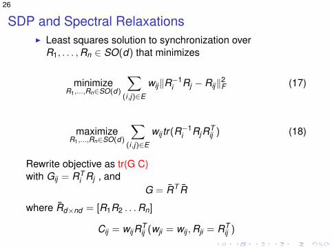
SDP and Spectral RelaxationsI Least squares solution to synchronization over
R1, . . . ,Rn ∈ SO(d) that minimizes
minimizeR1,...,Rn∈SO(d)
∑(i,j)∈E
wij‖R−1i Rj − Rij‖2F (17)
maximizeR1,...,Rn∈SO(d)
∑(i,j)∈E
wij tr(R−1i RjRT
ij ) (18)
Rewrite objective as tr(G C)with Gij = RT
i Rj , andG = RT R
where Rd×nd = [R1R2 . . .Rn]
Cij = wijRTij (wji = wij ,Rji = RT
ij )

27
I SDP Relaxation (Singer, 2011)
maximizeG
tr(GC)
subject to G � 0Gii = Id , for i = 1, . . .n[rank(G) = d ]
[det(Gij) = 1, for i , j = 1, . . .n] (19)
I Spectral Relaxation: via the graph Connection Laplacian L
Let W ∈ Rnd×nd with blocks Wij = wijRijLet D ∈ Rnd×nd diagonal with Dii = di Id where di =
∑j wij
L = D −W , with LRT = 0Recover the rotations from the bottom d eigenvectors of L +SVD for rounding in the noisy case.

28
The Graph Realization Problem
−0.3 −0.2 −0.1 0 0.1 0.2 0.3
−0.2
−0.1
0
0.1
0.2
−0.3 −0.2 −0.1 0 0.1 0.2 0.3
−0.2
−0.1
0
0.1
0.2
Figure: Original US map with n = 1090 and the measurement graphwith sensing radius ρ = 0.032.
−4−3
−2−1
01
23
−3
−2
−1
0
1
2
3
−0.5
0
0.5
Y
X
Z
Figure: BRIDGE-DONUT data set of n = 500 points in R3 and themeasurement graph of radius ρ = 0.92.

29
The Graph Realization Problem in Rd
I Graph G = (V ,E), |V | = n nodesI Set of distances lij = lji ∈ R for every pair (i , j) ∈ EI Goal: find a d-dimensional embedding p1, . . .pn ∈ Rd s.t.
||pi − pj || = lij , for all (i , j) ∈ E
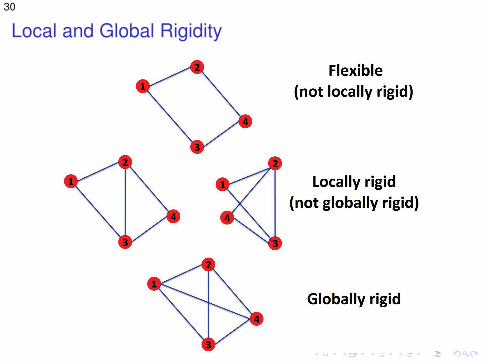
I If the solution is unique (up to a rigid motion), then graph isglobally rigid (uniquely realizable)
I Noise dij = lij(1 + εij) where εij ∼ Uniform([−η, η])
I Disc graph model with sensing radius ρ, dij ≤ ρ iff (i , j) ∈ E
Practical applications:I Input: sparse noise subset of pairwise distances between
sensors/atomsI Output: d-dimensional coordinates of sensors/atoms
30
Local and Global Rigidity
31
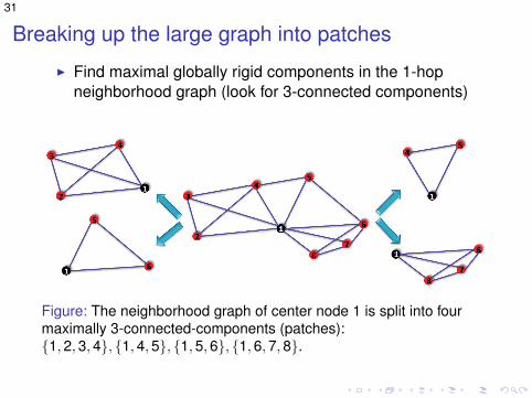
Breaking up the large graph into patches
I Find maximal globally rigid components in the 1-hopneighborhood graph (look for 3-connected components)
Figure: The neighborhood graph of center node 1 is split into fourmaximally 3-connected-components (patches):{1,2,3,4}, {1,4,5}, {1,5,6}, {1,6,7,8}.
32
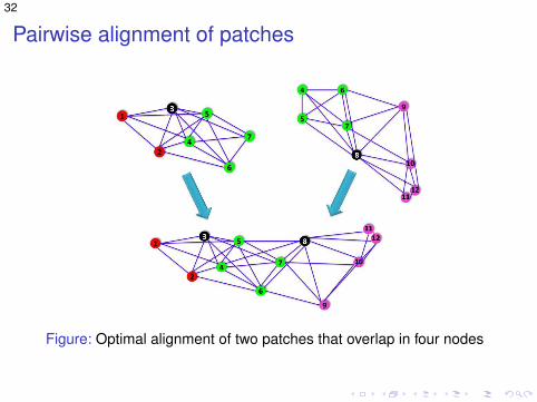
Pairwise alignment of patches
Figure: Optimal alignment of two patches that overlap in four nodes
33
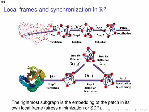
Local frames and synchronization in Rd
The rightmost subgraph is the embedding of the patch in itsown local frame (stress minimization or SDP).
34
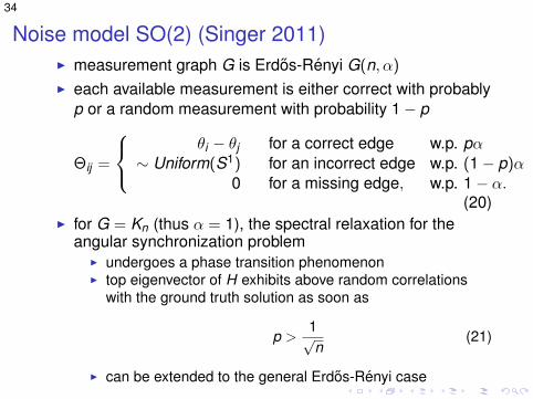
Noise model SO(2) (Singer 2011)I measurement graph G is Erdos-Renyi G(n, α)
I each available measurement is either correct with probablyp or a random measurement with probability 1− p
Θij =
θi − θj for a correct edge w.p. pα
∼ Uniform(S1) for an incorrect edge w.p. (1− p)α0 for a missing edge, w.p. 1− α.
(20)I for G = Kn (thus α = 1), the spectral relaxation for the
angular synchronization problemI undergoes a phase transition phenomenonI top eigenvector of H exhibits above random correlations
with the ground truth solution as soon as
p >1√n
(21)
I can be extended to the general Erdos-Renyi case

35
Spectral and SDP relaxations for SO(2)
I Build the n × n sparse Hermitian matrix H
Hij =
{eıθij if (i , j) ∈ E0 if (i , j) /∈ E .
(22)
I Singer considers the following maximization problem
maximizeθ1,...,θn∈[0,2π)
n∑i,j=1
e−ιθi Hijeιθj (23)
I gets incremented by +1 whenever an assignment ofangles θi and θj perfectly satisfies the given edgeconstraint Θij = θi − θj mod 2π (i.e., for a good edge),
I the contribution of an incorrect assignment (i.e., of a badedge) will be uniformly distributed on the unit circle
36
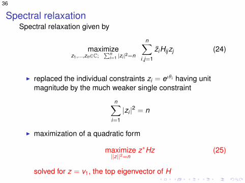
Spectral relaxationSpectral relaxation given by
maximizez1,...,zn∈C;
∑ni=1 |zi |2=n
n∑i,j=1
ziHijzj (24)
I replaced the individual constraints zi = eιθi having unitmagnitude by the much weaker single constraint
n∑i=1
|zi |2 = n
I maximization of a quadratic form
maximize||z||2=n
z∗Hz (25)
solved for z = v1, the top eigenvector of H
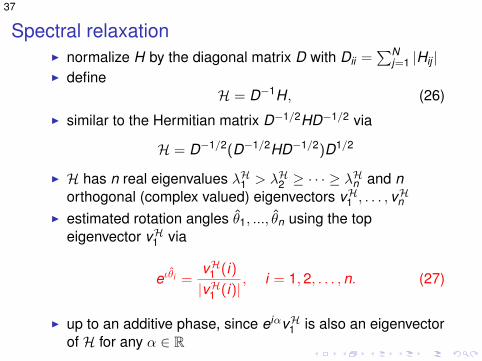
37
Spectral relaxationI normalize H by the diagonal matrix D with Dii =
∑Nj=1 |Hij |
I defineH = D−1H, (26)
I similar to the Hermitian matrix D−1/2HD−1/2 via
H = D−1/2(D−1/2HD−1/2)D1/2
I H has n real eigenvalues λH1 > λH2 ≥ · · · ≥ λHn and northogonal (complex valued) eigenvectors vH1 , . . . , v
Hn
I estimated rotation angles θ1, ..., θn using the topeigenvector vH1 via
eιθi =vH1 (i)|vH1 (i)|
, i = 1,2, . . . ,n. (27)
I up to an additive phase, since eiαvH1 is also an eigenvectorof H for any α ∈ R
38
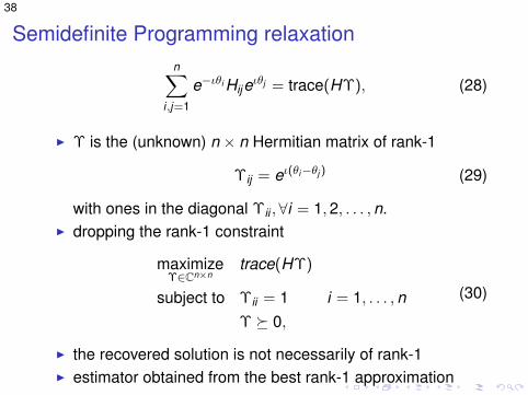
Semidefinite Programming relaxationn∑
i,j=1
e−ιθi Hijeιθj = trace(HΥ), (28)
I Υ is the (unknown) n × n Hermitian matrix of rank-1
Υij = eι(θi−θj ) (29)
with ones in the diagonal Υii ,∀i = 1,2, . . . ,n.I dropping the rank-1 constraint
maximizeΥ∈Cn×n
trace(HΥ)
subject to Υii = 1 i = 1, . . . ,nΥ � 0,
(30)
I the recovered solution is not necessarily of rank-1I estimator obtained from the best rank-1 approximation

39
Synchronization-based ranking
−0.8 −0.6 −0.4 −0.2 0 0.2 0.4 0.6 0.8 10
0.2
0.4
0.6
0.8
1
10 20 30 40 50 60 70 80 90 100
(a)
−0.5 0 0.5
−0.4
−0.2
0
0.2
0.4
0.6
0.8
20 40 60 80 100
(b)
Figure: (a) Equidistant mapping of the rankings 1,2, . . . ,n around halfa circle, for n = 100, where the rank of the i th player is i . (b) Therecovered solution at some random rotation, motivating the stepwhich computes the best circular permutation of the recoveredrankings, which minimizes the number of upsets with respect to theinitially given pairwise measurements.
40
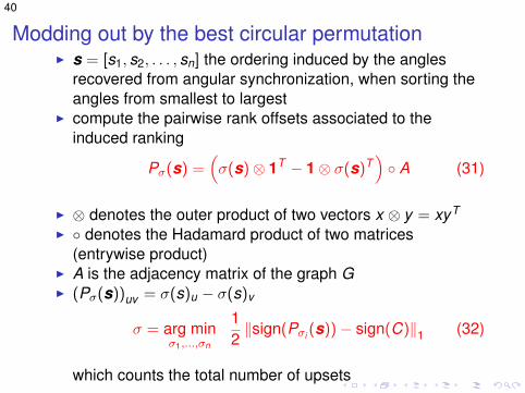
Modding out by the best circular permutationI s = [s1, s2, . . . , sn] the ordering induced by the angles
recovered from angular synchronization, when sorting theangles from smallest to largest
I compute the pairwise rank offsets associated to theinduced ranking
Pσ(s) =(σ(s)⊗ 1T − 1⊗ σ(s)T
)◦ A (31)
I ⊗ denotes the outer product of two vectors x ⊗ y = xyT
I ◦ denotes the Hadamard product of two matrices(entrywise product)
I A is the adjacency matrix of the graph GI (Pσ(s))uv = σ(s)u − σ(s)v
σ = arg minσ1,...,σn
12‖sign(Pσi (s))− sign(C)‖1 (32)
which counts the total number of upsets

41
The Sync-Rank AlgorithmRequire: Matrix C pairwise comparisons
1: Map all rank offsets Cij to an angle Θij ∈ [0,2πδ)
Cij 7→ Θij := 2πδCij
n − 1(33)
We choose δ = 12 , and hence Θij := π
Cijn−1 .
2: Build the n × n Hermitian matrix H withHij = eıθij , if (i , j) ∈ E , and Hij = 0 otherwise
3: Solve the ASP via its spectral or SDP relaxation, anddenote the recovered solution byri = eıθi =
vR1 (i)|vR
1 (i)| , i = 1,2, . . . ,n
4: Extract the corresponding set of angles θ1, . . . , θn ∈ [0,2π)from r1, . . . , rn, as in (27).
5: Compute the best circular permutation σ∗ that minimizesthe number of upsets in the induced ordering
6: Output as a final solution the ranking induced by thecircular permutation σ∗.
Figure: Summary of the Sync-Rank Algorithm.
42
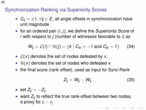
Synchronization Ranking via Superiority Scores
I Cij = ±1,∀ij ∈ E , all angle offsets in synchronization haveunit magnitude
I for an ordered pair (i , j), we define the Superiority Score ofi with respect to j (number of witnesses favorable to i) as
Wij = L(i) ∩H(j) = {k | Cik = −1 and Cjk = 1} (34)
I L(x) denotes the set of nodes defeated by x ,I H(x) denotes the set of nodes who defeated xI the final score (rank offset), used as input for Sync-Rank
Zij = Wji −Wij (35)
I set Zji = −Zij
I want Zij to reflect the true rank-offset between two nodes,a proxy for ri − rj
43
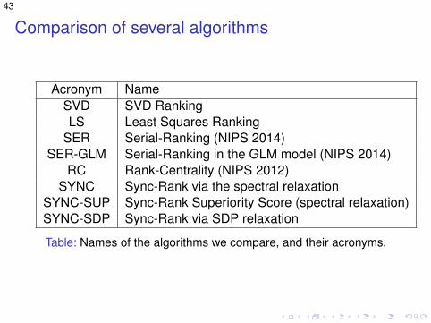
Comparison of several algorithms
Acronym NameSVD SVD RankingLS Least Squares Ranking
SER Serial-Ranking (NIPS 2014)SER-GLM Serial-Ranking in the GLM model (NIPS 2014)
RC Rank-Centrality (NIPS 2012)SYNC Sync-Rank via the spectral relaxation
SYNC-SUP Sync-Rank Superiority Score (spectral relaxation)SYNC-SDP Sync-Rank via SDP relaxation
Table: Names of the algorithms we compare, and their acronyms.

44
ERO, η = 0
20 40 60 80 1000
20
40
60
80
100
LS: τ = 0 , κ = 1
Ground truth rank
Recovere
d r
ank
(a) LS
20 40 60 80 1000
20
40
60
80
100
SVD: τ = 0.036 , κ = 0.929
Ground truth rank
Recovere
d r
ank
(b) SVD
20 40 60 80 1000
20
40
60
80
100
SER: τ = 0.028 , κ = 0.944
Ground truth rank
Recovere
d r
ank
(c) SER
20 40 60 80 1000
20
40
60
80
100
SER−GLM: τ = 0.034 , κ = 0.933
Ground truth rank
Recovere
d r
ank
(d) SER-GLM
20 40 60 80 1000
20
40
60
80
100
RC: τ = 0.001 , κ = 0.998
Ground truth rank
Recovere
d r
ank
(e) RC
20 40 60 80 1000
20
40
60
80
100
SYNC−EIG : τ = 0 , κ = 1
Ground truth rankR
ecovere
d r
ank
(f) SYNC-EIG

45
ERO, η = 0.35
20 40 60 80 1000
20
40
60
80
100
LS: τ = 0.088 , κ = 0.825
Ground truth rank
Recovere
d r
ank
(a) LS
20 40 60 80 1000
20
40
60
80
100
SVD: τ = 0.099 , κ = 0.802
Ground truth rank
Recovere
d r
ank
(b) SVD
20 40 60 80 1000
20
40
60
80
100
SER: τ = 0.114 , κ = 0.772
Ground truth rank
Recovere
d r
ank
(c) SER
20 40 60 80 1000
20
40
60
80
100
SER−GLM: τ = 0.152 , κ = 0.697
Ground truth rank
Recovere
d r
ank
(d) SER-GLM
20 40 60 80 1000
20
40
60
80
100
RC: τ = 0.088 , κ = 0.823
Ground truth rank
Recovere
d r
ank
(e) RC
20 40 60 80 1000
20
40
60
80
100
SYNC−EIG : τ = 0.027 , κ = 0.945
Ground truth rankR
ecovere
d r
ank
(f) SYNC-EIG

46
ERO, η = 0.75
20 40 60 80 1000
20
40
60
80
100
LS: τ = 0.195 , κ = 0.61
Ground truth rank
Recovere
d r
ank
(a) LS
20 40 60 80 1000
20
40
60
80
100
SVD: τ = 0.308 , κ = 0.383
Ground truth rank
Recovere
d r
ank
(b) SVD
20 40 60 80 1000
20
40
60
80
100
SER: τ = 0.444 , κ = 0.112
Ground truth rank
Recovere
d r
ank
(c) SER
20 40 60 80 1000
20
40
60
80
100
SER−GLM: τ = 0.394 , κ = 0.212
Ground truth rank
Recovere
d r
ank
(d) SER-GLM
20 40 60 80 1000
20
40
60
80
100
RC: τ = 0.195 , κ = 0.61
Ground truth rank
Recovere
d r
ank
(e) RC
20 40 60 80 1000
20
40
60
80
100
SYNC−EIG : τ = 0.152 , κ = 0.696
Ground truth rankR
ecovere
d r
ank
(f) SYNC-EIG

47
Kendall distance
I measure accuracy using the popular Kendall distanceI counts the number of pairs of candidates that are ranked in
different order (flips), in the two permutations (the originalone and the recovered one)
κ(π1, π2) =|{(i , j) : i < j , [π1(i) < π1(j) ∧ π2(i) > π2(j)] }(n
2
)∨ [π1(i) > π1(j) ∧ π2(i) < π2(j)]}|
=nr .flips(n
2
) (36)
I we compute the Kendall distance on a logarithmic scale

48
Rank of the SDP solution (cardinal measurements)
0 5 10 151
1.5
2
2.5
3
3.5
η
avera
ge r
ank o
f th
e S
DP
(a) p = 0.2, MUN
0 5 10 151
1.2
1.4
1.6
1.8
2
η
avera
ge r
ank o
f th
e S
DP
(b) p = 0.5, MUN
0 5 10 151
1.1
1.2
1.3
1.4
1.5
1.6
1.7
1.8
η
avera
ge r
ank o
f th
e S
DP
(c) p = 1, MUN
0 0.2 0.4 0.6 0.81
1.5
2
2.5
3
3.5
4
4.5
5
η
avera
ge r
ank o
f th
e S
DP
(d) p = 0.2, ERO
0 0.2 0.4 0.6 0.81
1.5
2
2.5
3
3.5
4
4.5
5
η
avera
ge r
ank o
f th
e S
DP
(e) p = 0.5, ERO
0 0.2 0.4 0.6 0.81
1.5
2
2.5
3
3.5
4
4.5
5
η
avera
ge r
ank o
f th
e S
DP
(f) p = 1, ERO

49
Multiplicative Uniform Noise MUN(n = 200,p = 0.2, η)
0 5 10 15 20−6
−5
−4
−3
−2
−1
0
η
log(K
endall
Dis
tance)
SVD
LS
SER
SYNC
SER−GLM
SYNC−SUP
SYNC−SDP
RC

50
Multiplicative Uniform Noise MUN(n = 200,p = 0.5, η)
0 5 10 15 20−7
−6
−5
−4
−3
−2
−1
0
η
log(K
endall
Dis
tance)
SVD
LS
SER
SYNC
SER−GLM
SYNC−SUP
SYNC−SDP
RC
51
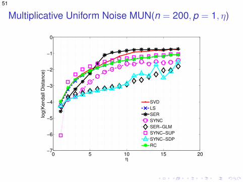
Multiplicative Uniform Noise MUN(n = 200,p = 1, η)
0 5 10 15 20−7
−6
−5
−4
−3
−2
−1
0
η
log(K
endall
Dis
tance)
SVD
LS
SER
SYNC
SER−GLM
SYNC−SUP
SYNC−SDP
RC

52
Erdos-Renyi Outliers ERO(n = 200,p = 0.2, η)
0 0.2 0.4 0.6 0.8 1−6
−5
−4
−3
−2
−1
0
η
log(K
endall
Dis
tance)
SVD
LS
SER
SYNC
SER−GLM
SYNC−SUP
SYNC−SDP
RC

53
Erdos-Renyi Outliers ERO(n = 200,p = 0.5, η)
0 0.2 0.4 0.6 0.8 1−7
−6
−5
−4
−3
−2
−1
0
η
log(K
endall
Dis
tance)
SVD
LS
SER
SYNC
SER−GLM
SYNC−SUP
SYNC−SDP
RC

54
Erdos-Renyi Outliers ERO(n = 200,p = 1, η)
0 0.2 0.4 0.6 0.8 1−7
−6
−5
−4
−3
−2
−1
0
η
log(K
endall
Dis
tance)
SVD
LS
SER
SYNC
SER−GLM
SYNC−SUP
SYNC−SDP
RC

55
Rank Aggregation
Figure: Multiple rating systems, each one providing its own pairwisecomparisons matrix, C(i), i = 1, . . . , k

56
Naive approach A: solve individually each of C(i), i = 1, . . . , k ,producing k possible rankings
r (i)1 , . . . , r (i)
n , i = 1, . . . , k (37)
and average out the resulting rankings.
Naive approach B: first average out all given data
C =C(1) + C(2) + . . .+ C(k)
k(38)
and extract a final ranking from C.
57
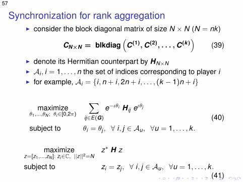
Synchronization for rank aggregationI consider the block diagonal matrix of size N × N (N = nk )
CN×N = blkdiag(
C(1),C(2), . . . ,C(k))
(39)
I denote its Hermitian counterpart by HN×NI Ai , i = 1, . . . ,n the set of indices corresponding to player iI for example, Ai = {i ,n + i ,2n + i , . . . , (k − 1)n + i}
maximizeθ1,...,θN ; θi∈[0,2π)
∑ij∈E(G)
e−ιθi H ij eιθj
subject to θi = θj , ∀ i , j ∈ Au, ∀u = 1, . . . , k .(40)
maximizez=[z1,...,zN ]: zi∈C, ||z||2=N
z∗ H z
subject to zi = zj , ∀ i , j ∈ Au, ∀u = 1, . . . , k .(41)

58
Synchronization for rank aggregation
maximizeΥ∈CN×N
Trace(HΥ)
subject to Υij = 1 if i , j ∈ Au, u = 1, . . . , kΥ � 0,
(42)
which is expensive...However, note that:
k∑u=1
∑ij∈E(G)
e−ιθi Θ(u)ij eιθj =
∑ij∈E(G)
e−ιθi
(k∑
u=1
eιΘ(u)ij
)eιθj
=∑
ij∈E(G)
e−ιθi Hijeιθj (43)
where
H =k∑
u=1
H(u) (44)
59
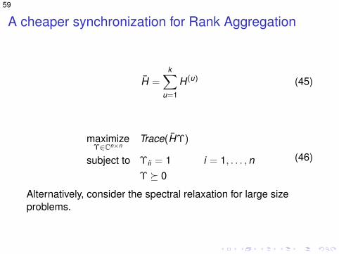
A cheaper synchronization for Rank Aggregation
H =k∑
u=1
H(u) (45)
maximizeΥ∈Cn×n
Trace(HΥ)
subject to Υii = 1 i = 1, . . . ,nΥ � 0
(46)
Alternatively, consider the spectral relaxation for large sizeproblems.
60
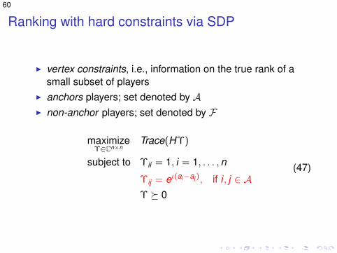
Ranking with hard constraints via SDP
I vertex constraints, i.e., information on the true rank of asmall subset of players
I anchors players; set denoted by AI non-anchor players; set denoted by F
maximizeΥ∈Cn×n
Trace(HΥ)
subject to Υii = 1, i = 1, . . . ,n
Υij = eι(ai−aj ), if i , j ∈ AΥ � 0
(47)

61
Ranking with hard constraints via SDP
Figure: Left: Searching for the best cyclic shift of the free players,shown in red. The black nodes denote the anchor players, whoserank is known and stays fixed. Right: The ground truth ranking.
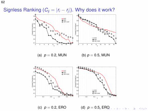
62
Signless Ranking (Cij = |ri − rj |). Why does it work?
0 2 4 6 8 10 12 14 16
0.1
0.2
0.3
0.4
0.5
0.6
0.7
0.8
η
| K
endall
Corr
ela
tion |
SVD
SER
SER−GLM
(a) p = 0.2, MUN
0 2 4 6 8 10 12 14 16
0.4
0.5
0.6
0.7
0.8
0.9
η
| K
endall
Corr
ela
tion |
SVD
SER
SER−GLM
(b) p = 0.5, MUN
0 0.2 0.4 0.6 0.8
0.1
0.2
0.3
0.4
0.5
0.6
0.7
0.8
η
| K
endall
Corr
ela
tion |
SVD
SER
SER−GLM
(c) p = 0.2, ERO
0 0.2 0.4 0.6 0.8
0.1
0.2
0.3
0.4
0.5
0.6
0.7
0.8
0.9
η
| K
endall
Corr
ela
tion |
SVD
SER
SER−GLM
(d) p = 0.5, ERO
63
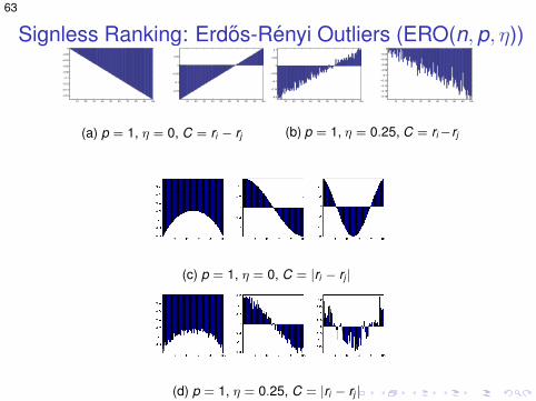
Signless Ranking: Erdos-Renyi Outliers (ERO(n,p, η))
10 20 30 40 50 60 70 80 90 100
−0.16
−0.14
−0.12
−0.1
−0.08
−0.06
−0.04
−0.02
0
10 20 30 40 50 60 70 80 90 100
−0.15
−0.1
−0.05
0
0.05
(a) p = 1, η = 0, C = ri − rj
10 20 30 40 50 60 70 80 90 100
−0.2
−0.15
−0.1
−0.05
0
0.05
0.1
10 20 30 40 50 60 70 80 90 100
−0.18
−0.16
−0.14
−0.12
−0.1
−0.08
−0.06
−0.04
−0.02
0
(b) p = 1, η = 0.25, C = ri−rj
(c) p = 1, η = 0, C = |ri − rj |
(d) p = 1, η = 0.25, C = |ri − rj |
64
Clustering with constraints
I important problem in machine learning and data miningI information about an application task comes in the form of
both data and domain knowledgeI domain knowledge is specified as a set of soft
I must-link (ML) constraintsI cannot-link (CL) constraints

65
A schematic overview of our approach
DataMLconstraints
CLconstraints
DiscreteOp1miza1onproblem
SpectralRelaxa1on
EmbeddingL
Lx=λHx ClusteringH
66
Our contribution
I a principled spectral approach for constrained clusteringI reduces to a generalized eigenvalue problem for which
both matrices are LaplaciansI guarantees for the quality of the clusters (for k = 2)I nearly-linear time implementationI outperforms existing methods both in speed and qualityI can deal with problems at least two orders of magnitude
higher than beforeI solves data sets with millions of points in less than 2
minutes, on very modest hardware

67
Related literature
I Rangapuram, S. S. and Hein, M. (2012). Constrained1-spectral clustering. In AISTATS, pages 1143-1151(COSC)
I Wang, X., Qian, B., and Davidson, I. (2012). Improvingdocument clustering using automated machine translation.CIKM 12
I reduces constrained clustering to a generalized eigenvalueproblem
I resulting problem is indefinite and the method requires thecomputation of a full eigenvalue decomposition
68
Constrained clustering problem definition1. GD: data graph which contains a given number of k
clusters that we seek to findI GD = (V ,ED,wD), with edge weights wD ≥ 0 indicating the
level of ‘affinity’ of their endpoints2. GML knowledge graph; an edge indicates that its two
endpoints should be in the same cluster3. GCL knowledge graph; an edge indicates that its two
endpoints should be in different cluster
I weight of a constraint edge indicates the level of beliefI prior knowledge does not have to be exact or even
self-consistent (hence soft constraints)I to conform with prior literature, use existing terminology of
‘must link’ (ML) and ‘cannot link’ (CL) constraintsGoal: find k disjoint clusters in GD obtained via
I cutting a small number of edges in the data graph GDI while simultaneously respecting as much as possible the
constraints in the knowledge graphs GML and GCL

69
Re-thinking constraints
I numerous approaches pursued within the constrainedspectral clustering framework
I although distinct, they share a common point of view:constraints are viewed as entities structurally extraneous tothe basic spectral formulation
I leads to modifications/extensions with mathematicalfeatures that are often complicated
I a key fact is overlooked:Standard clustering is a special case of constrainedclustering with implicit soft ML and CL constraints.
I recall the optimization in the standard method (NCUT)
φ = minS⊆V
cutGD (S, S)
vol(S)vol(S)/vol(V )
70
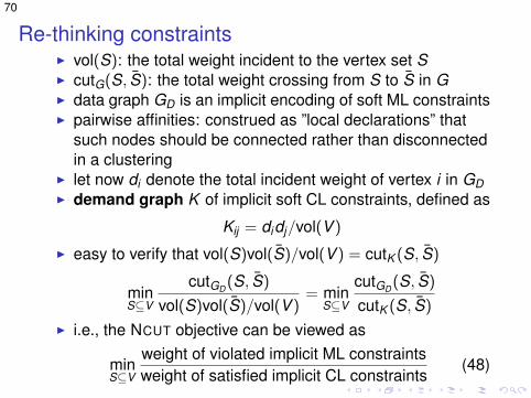
Re-thinking constraintsI vol(S): the total weight incident to the vertex set SI cutG(S, S): the total weight crossing from S to S in GI data graph GD is an implicit encoding of soft ML constraintsI pairwise affinities: construed as ”local declarations” that
such nodes should be connected rather than disconnectedin a clustering
I let now di denote the total incident weight of vertex i in GDI demand graph K of implicit soft CL constraints, defined as
Kij = didj/vol(V )
I easy to verify that vol(S)vol(S)/vol(V ) = cutK (S, S)
minS⊆V
cutGD (S, S)
vol(S)vol(S)/vol(V )= min
S⊆V
cutGD (S, S)
cutK (S, S)
I i.e., the NCUT objective can be viewed as
minS⊆V
weight of violated implicit ML constraintsweight of satisfied implicit CL constraints
(48)

71
Graph LaplaciansI G = (V ,E ,w) is a graph with non-negative weights wI the combinatorial Laplacian L of G is defined by
L = D −W : Lij =
{−wij , if i = j∑
j 6=i wij , ifi 6= j
I L satisfies the following basic identity for all vectors x
xT L x =∑i,j
wij(xi − xj)2 (49)
I given a cluster C ⊆ V , define a cluster indicator vectorxC(i) = 1 if i ∈ C and xC(i) = 0 otherwise. We have:
xTC L xC = cutG(C, C) (50)
I cutG(C, C) = the total weight crossing from C to C in G

72
The optimization problem
I input: two weighted graphs, the must-link constraints G,and the cannot-link constraints H
I objective: partition V into k disjoint clusters Ci .I define an individual measure of badness for each cluster Ci
φi(G,H) =cutG(Ci , Ci)
cutH(Ci , Ci)(51)
I numerator = total weight of the violated ML constraints,because cutting one such constraint violates it.
I denominator = total weight of the satisfied CL constraints,because cutting one such constraint satisfies it
I the minimization of the individual badness is a sensibleobjective

73
The optimization problemI find clusters C1, . . . ,Ck that minimize the maximum
badness, i.e. solve the following problem
Φk = min maxiφi (52)
I can be captured in terms of LaplaciansI xCi : indicator vector for cluster i
φi(G,H) =xT
CiLGxCi
xTCi
LHxCi
I solving the minimization problem in (52) amounts to findingk vectors in {0,1}n with disjoint support
I optimization problem may not be well-defined if there arevery few CL constraints in H
I can be detected easily and the user can be notifiedI the merging phase takes automatically care of this caseI we assume that the problem is well-defined

74
Spectral RelaxationI to relax the problem we instead look for k vectors in
y1, . . . , yk ∈ Rn, such that for all i 6= j , we have yiLHyj = 0I these LH -orthogonality constraints can be viewed as a
relaxation of the disjointness requirementI their particular form is motivated by the fact that they
directly give rise to a generalized eigenvalue problemI the k vectors yi that minimize the maximum among the k
Rayleigh quotients
(yTi LGyi)/(yT
i LHyi)
are precisely the generalized eigenvectors correspondingto the k smallest eigenvalues of
LGx = λLHx
I if H is the demand graph K , the problem is identical to thestandard problem LGx = λDx , where D = diag(LG), since
I LK = D − ddT/(dT 1)I eigenvectors of LGx = λDx are d-orthogonal, where d is
vector of degrees in G

75
Spectral Relaxation
I this fact is well understood and follows from ageneralization of the min-max characterization of theeigenvalues for symmetric matrices
I details can be found for instance in Stewart and Sun,Matrix Perturbation Theory, 1990
I note that H does not have to be connectedI since we are looking for a minimum, the optimization
function avoids vectors that are in the null space of LH
I ⇒ no restriction needs to be placed on x so that theeigenvalue problem is well defined, other than it cannot bethe constant vector (which is in the null space of both LGand LH ), assuming without loss of generality that G isconnected

76
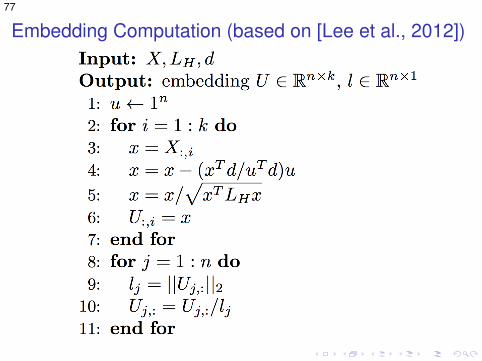
The embedding
I let X be the n × k matrix of the first k generalizedeigenvectors for LGx = λLHx
I the embedding borrows ideas from
Lee, Gharan, Trevisan, ”Multi-way Spectral Partitioning andHigher-order Cheeger Inequalities”, STOC ’12
77
Embedding Computation (based on [Lee et al., 2012])
78
Computing Eigenvectors
I spectral algorithms based on eigenvector embeddings donot require the exact eigenvectors, but only approximations
I the computation of the approximate generalizedeigenvectors for LGx = λLHx is most time-consuming
I the asymptotically fastest known algorithm for the problemruns in O(km log2 m) time, and combines
I a fast Laplacian linear system solver (Koutis et al. 2011)I a standard power method (Glob and Loan 1996)
I in practice, we use the combinatorial multigrid solver(Koutis et al. 2011) which empirically runs in O(m) time
I the solver provides an approximate inverse for LG which inturn is used with the preconditioned eigenvalue solverLOBPCG (Knyazev 2001)

79
Merging constraints: a simple heuristic
I often, users provide unweighted constraints GML and GCL
I construct two weighted graphs GML and GCL, as follows: ifedge (i , j) is a constraint, we take its weight in thecorresponding graph to be didj/(dmindmax), where didenotes the total incident weight of vertex i ,
I dmin,dmax the minimum and maximum among the di ’sI let G = GD + GML and H = K/n + GCL
I K is the demand graphI include small copy of K in H to render the problem
well-defined in all cases of user input
80
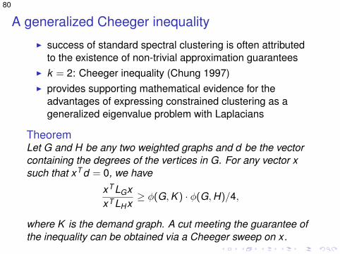
A generalized Cheeger inequality
I success of standard spectral clustering is often attributedto the existence of non-trivial approximation guarantees
I k = 2: Cheeger inequality (Chung 1997)I provides supporting mathematical evidence for the
advantages of expressing constrained clustering as ageneralized eigenvalue problem with Laplacians
TheoremLet G and H be any two weighted graphs and d be the vectorcontaining the degrees of the vertices in G. For any vector xsuch that xT d = 0, we have
xT LGxxT LHx
≥ φ(G,K ) · φ(G,H)/4,
where K is the demand graph. A cut meeting the guarantee ofthe inequality can be obtained via a Cheeger sweep on x.
81
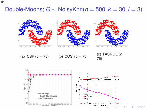
Double-Moons; G ∼ NoisyKnn(n = 500, k = 30, l = 3)
−10 −5 0 5 10 15 20
−5
0
5
10
(a) CSP (c = 75)
−10 −5 0 5 10 15 20
−5
0
5
10
(b) COSf (c = 75)
−10 −5 0 5 10 15 20
−5
0
5
10
(c) FAST-GE (c =75)
10 25 50 75 100 125 150 175 200 225 250 275 300 325 3500.7
0.75
0.8
0.85
0.9
0.95
1
1.05
Number of Constraints
Ra
nd
In
de
x
CSP−sign
FAST−GE−kmeans
COSf−kmeans
(d) Accuracy (e) Running times (log)
82
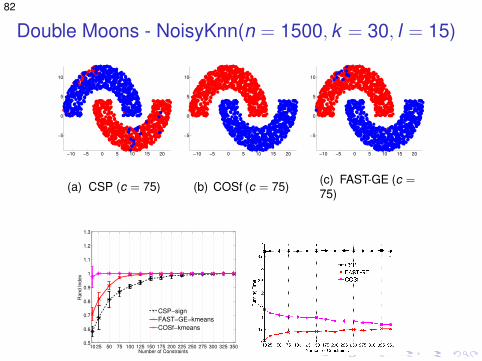
Double Moons - NoisyKnn(n = 1500, k = 30, l = 15)
−10 −5 0 5 10 15 20
−5
0
5
10
(a) CSP (c = 75)
−10 −5 0 5 10 15 20
−5
0
5
10
(b) COSf (c = 75)
−10 −5 0 5 10 15 20
−5
0
5
10
(c) FAST-GE (c =75)
10 25 50 75 100 125 150 175 200 225 250 275 300 325 3500.5
0.6
0.7
0.8
0.9
1
1.1
1.2
1.3
Number of Constraints
Ra
nd
In
de
x
CSP−sign
FAST−GE−kmeans
COSf−kmeans
(d) Accuracy (e) Running times (log)
83
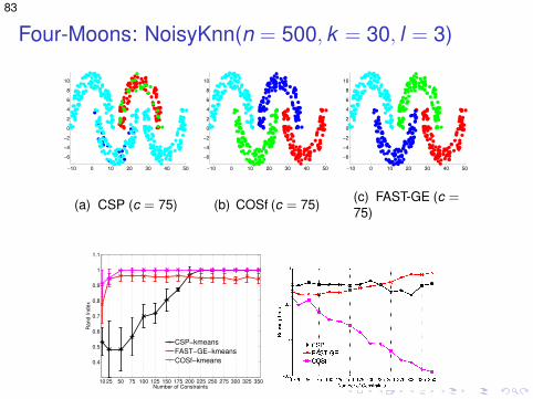
Four-Moons: NoisyKnn(n = 500, k = 30, l = 3)
−10 0 10 20 30 40 50
−6
−4
−2
0
2
4
6
8
10
(a) CSP (c = 75)
−10 0 10 20 30 40 50
−6
−4
−2
0
2
4
6
8
10
(b) COSf (c = 75)
−10 0 10 20 30 40 50
−6
−4
−2
0
2
4
6
8
10
(c) FAST-GE (c =75)
10 25 50 75 100 125 150 175 200 225 250 275 300 325 350
0.4
0.5
0.6
0.7
0.8
0.9
1
1.1
Number of Constraints
Ra
nd
In
de
x
CSP−kmeans
FAST−GE−kmeans
COSf−kmeans
(d) Accuracy (e) Running times (log)
84
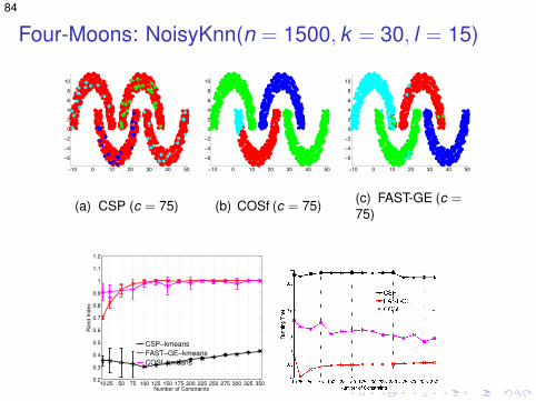
Four-Moons: NoisyKnn(n = 1500, k = 30, l = 15)
−10 0 10 20 30 40 50
−6
−4
−2
0
2
4
6
8
10
(a) CSP (c = 75)
−10 0 10 20 30 40 50
−6
−4
−2
0
2
4
6
8
10
(b) COSf (c = 75)
−10 0 10 20 30 40 50
−6
−4
−2
0
2
4
6
8
10
(c) FAST-GE (c =75)
10 25 50 75 100 125 150 175 200 225 250 275 300 325 3500.2
0.3
0.4
0.5
0.6
0.7
0.8
0.9
1
1.1
1.2
Number of Constraints
Ra
nd
In
de
x
CSP−kmeans
FAST−GE−kmeans
COSf−kmeans
(d) Accuracy (e) Running times (log)
85
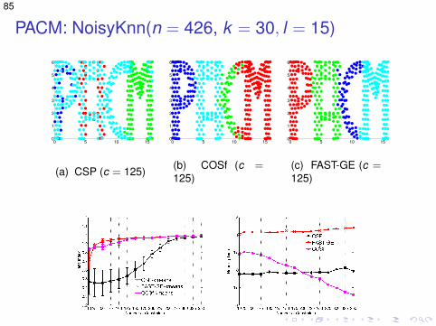
PACM: NoisyKnn(n = 426, k = 30, l = 15)
0 5 10 150
1
2
3
4
5
6
(a) CSP (c = 125)
0 5 10 150
1
2
3
4
5
6
(b) COSf (c =125)
0 5 10 150
1
2
3
4
5
6
(c) FAST-GE (c =125)
(d) Accuracy (e) Running times (log)
86
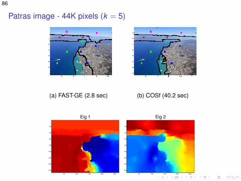
Patras image - 44K pixels (k = 5)
(a) FAST-GE (2.8 sec) (b) COSf (40.2 sec)
Eig 1
50 100 150 200 250
20
40
60
80
100
120
140
160
(c) FAST-GE: Eigen-vector 1
Eig 2
50 100 150 200 250
20
40
60
80
100
120
140
160
(d) FAST-GE: Eigen-vector 2
87
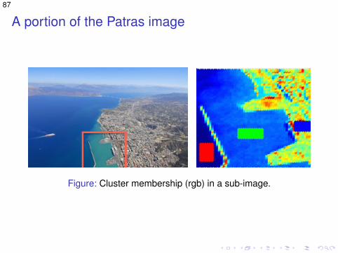
A portion of the Patras image
Figure: Cluster membership (rgb) in a sub-image.

88
A comparison of all methods
10 20 30 40
10
20
30
40
(a) COSC (b) CSP
(c) FAST-GE (d) FAST-GE
Figure: A comparison of COSC (row 1), CSP (row 2) and FAST-GE(row 3) for a sub-image of the Patras image, with three clusters. Theright column overlays the boundary on the actual image.
89
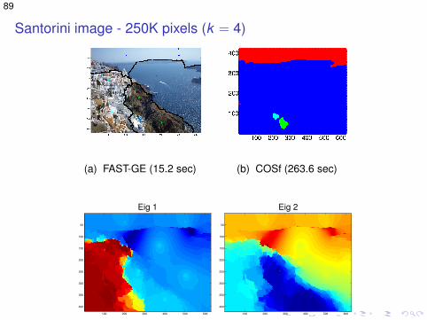
Santorini image - 250K pixels (k = 4)
(a) FAST-GE (15.2 sec) (b) COSf (263.6 sec)
Eig 1
100 200 300 400 500 600
50
100
150
200
250
300
350
400
(c) FAST-GE: Eig 1
Eig 2
100 200 300 400 500 600
50
100
150
200
250
300
350
400
(d) FAST-GE: Eig 2

90
Soccer image - ∼ 1.1 million pixels (k = 5)
200 400 600 800 1000 1200
100
200
300
400
500
600
700
800
900
(a) Clean image (b) FAST-GE (94 sec)
Eig 2
200 400 600 800 1000 1200
100
200
300
400
500
600
700
800
900
(c) FAST-GE (d) COSf (25 min)