Spectral Decomposition of Forms - University of...
49
Spectral Decomposition of Forms 1 Xiaohong Chen Department of Economics Yale University email: [email protected] Lars Peter Hansen Department of Economics University of Chicago email: [email protected] Jos´ e A. Scheinkman Department of Economics Princeton University email: [email protected] First Draft: October 2000 Current Draft: October 2007 1 We thank Anna Aslanyan, Henri Berestycki, E. Brian Davies, Nan Li, Gigliola Staffilani and Gauhar Turmuhambetova for useful conversations. Chen, Hansen and Scheinkman all acknowledge support from the National Science Foundation.
Transcript of Spectral Decomposition of Forms - University of...
Spectral Decomposition of Forms1
Xiaohong ChenDepartment of Economics
Yale Universityemail: [email protected]
Lars Peter HansenDepartment of Economics
University of Chicagoemail: [email protected]
Jose A. ScheinkmanDepartment of Economics
Princeton Universityemail: [email protected]
First Draft: October 2000Current Draft: October 2007
1We thank Anna Aslanyan, Henri Berestycki, E. Brian Davies, Nan Li, Gigliola Staffilaniand Gauhar Turmuhambetova for useful conversations. Chen, Hansen and Scheinkman allacknowledge support from the National Science Foundation.
Abstract
We investigate the spectral decomposition of symmetric forms. The forms are pa-
rameterized by weighting functions for levels and derivatives of a class of test func-
tions. Our interest in these forms is that they are associated with operator semi-
groups from underlying Markov processes. We establish the existence of a discrete
spectrum by restricting the weighting functions used in constructing the forms.
These weighting functions have explicit interpretations in the Markov environments
that interest us. They are built from the diffusion matrix, the stationary density
for the diffusion and a state dependent decay rate used in representing the Markov
semigroup. We provide primitive sufficient conditions for the existence of eigen-
functions, and we characterize the limiting behavior of the associated eigenvalues,
the objects used to quantify the incremental importance of the eigenfunctions. We
use our results to provide sufficient conditions for the spectral decomposition of
Feynman-Kac operators and Markov semigroups.
Key words and phrases. Markov semigroups, discrete spectrum, eigenvalue decay
rates, multivariate diffusion, quadratic form, Feynman-Kac operator.
1 Introduction
One parameter semigroups are used in a variety of settings to study dynamic be-
havior in Markovian environments. When there is nonlinear dependence of local
dynamics, spectral methods premised on eigenfunction decompositions are a valu-
able tool for linking the local dynamics, say evolution over an instant, to global
dynamics or evolution over long time horizons. In this paper we study spectral
decomposition using quadratic forms that embed operators. A quadratic form f is
expressed in terms of the gradients of functions. Specifically, the quadratic form is
f(φ,ψ) =12
∫Ω∇φ(x)′Σ(x)∇ψ(x)q(x)dx +
∫Ωφ(x)ψ(x)π(x)q(x)dx
where Σ is a state-dependent positive-definite matrix, q is a probability density,
π is a nonnegative weighting function, ∇ denotes the (weak) gradient operator
and Ω is the state space. The operator associated with such a form generates a
semigroup and the objects Σ, q and π have explicit interpretations as they relate to
the semigroup. We establish the existence of the simple eigenfunction structure (a
discrete spectrum) by imposing restrictions on (Σ, q, π).
When π is zero, in Chen et al. (2007) we obtain a method for extracting eigen-
functions of Markov diffusion processes from multivariate discrete-time low fre-
quency time series observations. We allow for π to be different from zero to ac-
commodate Feynman-Kac operators in which π becomes a state dependent decay
rate. Growth in the semigroup is accommodated by translating this decay rate by
a constant.
In this paper we do the following:
1. Formulate a sequence of optimization problems used to construct eigenfunc-
tions of the underlying form and the associated semigroup.

2. Give primitive sufficient conditions for the existence of these eigenfunctions
and provide bounds on the incremental importance of these components when
used in approximation.
3. Provide a reversible Markov diffusion process for the data generation that
supports this eigenfunction extraction method in conjunction with a state
dependent discount or decay rate.
4. Show that these sufficient conditions imply the existence of countably many
eigenvalues and eigenfunctions for a more general class of Markov diffusion
processes.
The rest of the paper is organized as follows. In Section 2 we introduce quadratic
forms on function spaces that will be used throughout our analysis. In Section 3 we
construct a sequence of functions that maximize second moments subject to orthog-
onality conditions and smoothness bounds given by the quadratic form f. These
functions are eigenfunctions of the form f. The results in Sections 4 and 5 relate the
eigenfunctions of forms to eigenfunctions of semigroups constructed from an under-
lying Markov process {xt} defined using the diffusion matrix Σ and the stationary
density q. If the constraints of the optimization problems satisfy a compactness cri-
teria, eigenfunctions exist. Section 6 is dedicated to deriving primitive conditions
that imply the compactness criteria. In contrast to the local drift conditions fea-
tured by Kontoyiannis and Meyn (2003), our conditions restrict in part the tails of
density q that governs long-run stochastic behavior. In this sense our work is com-
plementary to the existing literature by providing an alternative way to show that
the spectrum of the semigroup is discrete. In Section 7 we specialize the conditions
that imply compactness to the case when radial symmetry holds and discuss four
parameterized examples. We then present bounds on the rate of divergence of the
2
eigenvalues that are associated with the eigenfunctions. These bounds, in turn, are
bounds on the rate of convergence of the approximation errors that obtain when we
use eigenfunctions in approximation. Section 8 concludes by briefly comparing our
approach to those of others and discussing applications of our results. The appendix
contains the proofs.
2 Quadratic Forms
We consider two quadratic forms. We start with an open connected Ω ⊆ Rn. Let
q be a probability density on Ω with respect to Lebesgue measure. The implied
probability distribution is the population counterpart to the empirical distribution
of the data. Let L2 denote the space of Borel measurable square integrable functions
with respect to population probability distribution. The first form is the L2 inner
product, denoted as < φ,ψ >=∫Ω φ(x)ψ(x)q(x)dx. We use the corresponding norm
(‖φ‖2 =√< φ, φ >) to define an approximation criterion.
The second form is used to measure smoothness. Consider a (quadratic) form fo
defined on C2K , the space of twice continuously differentiable functions with compact
support in Ω, that can be parameterized in terms of the density q, a nonnegative
weighting function π and a positive definite matrix Σ = [σij ] that can depend on
the state:
fo(φ,ψ) =12
∫Ω
∑i,j
σij∂φ
∂yj
∂ψ
∂yiq +
∫Ωφ(x)ψ(x)π(x)q(x)dx. (1)
We assume
Assumption 2.1. q is a positive, continuously differentiable probability density on
Ω.
3
Assumption 2.2. Σ is a continuously differentiable, positive definite matrix func-
tion on Ω.1
Assumption 2.3. π is a continuous, nonnegative function on Ω.
While the fo is constructed in terms of the products Σq and πq, the density q will
play a distinct role when we consider extending the domain of the form to a larger
set of functions.
To study the case in which Ω is not compact, we will consider a particular closed
extension of the form fo. We extend the form fo to a larger domain H ⊂ L2 using
the notion of a weak derivative.
H.= {φ ∈ L2 :
∫(φ)2πq <∞, there exists g measurable, with
∫g′Σgq <∞,
and∫φ∇ψ = −
∫gψ, for all ψ ∈ C1
K}
The random vector g is unique (for each φ) and is referred to as the weak derivative
of φ.
From now on, for each φ in H we write ∇φ = g.2 For any pair of functions ψ
and φ in H we define:
f(φ,ψ) =12
∫Ω(∇φ)′Σ(∇ψ)q +
∫Ωφψπq,
which is an extension of fo. In H we use the inner product < φ,ψ >f=< φ,ψ >
+f(φ,ψ). In Appendix we prove that with this inner product H is complete (and1Assumptions 2.1 and 2.2 restrict the density q and the matrix Σ to be continuously differen-
tiable. As argued by Davies (1989) these restrictions can be replaced by a less stringent requirementthat entries of the matrix qΣ are locally (in L2(Lebesgue)), weakly differentiable. (See Theorem1.2.5.)
2Notice that H is constructed exactly as a weighted Sobolev space except that instead of requiringthat g ∈ L2, we require that Λg ∈ L2 where Λ is the square root of Σ. Also we use C1
K test functions.One can show, using mollifiers, that allowing for this larger set of test functions is equivalent tousing the more usual set of test functions, C∞
K (see Brezis (1983) Remark 1, page 150.)
4

hence a Hilbert space). Thus H is taken to be the domain D(f) of the form f .
Notice, in particular, that the unit function is in D(f).
3 Eigenfunctions
We show that the eigenfunctions of interest solve a sequence of constrained maxi-
mization problems where form is used to define the constraints.
Definition 3.1. : The function ψj is the jth nonlinear principal component for
j ≥ 1 if ψj solves:
maxφ
< φ, φ >
subject to
θ < φ, φ > +f(φ, φ) = 1
< ψs, φ > = 0, s = 1, ..., j − 1
for some θ > 0.
The choice of θ turns out to only alter the scale of the principal component.
The constraint set gets larger as θ declines to zero. Thus the maximized objective
increases as θ is reduced. While this is true, it turns out the maximizing choice of φ
does not depend on θ up to scale. This follows because the ranking over φ’s implied
by the ratio:< φ, φ >
θ < φ, φ > +f(φ, φ)
does not depend on the value of θ.
More formally, the problems in this sequence have a canonical structure:
5
Problem 3.1.
maxφ∈H
< φ, φ >
subject to:
θ < φ, φ > +f(φ, φ) ≤ 1
where H is a closed linear subspace of L2.
The solutions for alternative θ’s can be obtained by solving one such problem and
rescaling that solution to satisfy the alternative constraints with equality. Typically
we are only interested in the principal components up to a scale factor, so that the
magnitude of θ is not important.
In the special case in which π is constant, the first eigenfunction is identically
one, and as a consequence the remaining principal components have mean zero under
the probability distribution Q with density q.
To establish the existence of a solution to Problem 3.1, it suffices to suppose the
following:
Criterion 3.1. {φ ∈ D(f) : θf(φ, φ)+ < φ, φ >≤ 1} is precompact (has compact
closure) in L2.
The precompactness restriction guarantees that we may extract an L2 convergent
sequence in the constraint set, with objectives that approximate the supremum. The
limit point of convergent sequence used to approximate the supremum, however,
will necessarily be in the constraint set because the constraint set is convex and the
form is closed. We provide sufficient conditions for this compactness criterion in
the next section. The solutions to the sequence of optimization problems 3.1 are
eigenfunctions of the quadratic forms f .
6
Definition 3.2. An eigenfunction ψ of the quadratic form f satisfies:
f(φ,ψ) = δ < φ,ψ > (2)
for all φ ∈ D(f). The scalar δ is the corresponding eigenvalue.
Claim 3.1. A solution φ∗ to Problem 3.1 will also solve the eigenvalue problem:
< ψ,φ∗ >= λ[θ < ψ, φ∗ > +f(ψ, φ∗)]
for some positive λ and all ψ ∈ H.
The proof of this and other formal results in this paper are given in the appendix.
Since f is positive semidefinite, δ must be nonnegative. The principal components
extracted in the manner given in Problem 3.1 have eigenvalues δj that increase with
j. If we renormalize the eigenfunctions to have a unit second moment, the principal
components will be ordered by their smoothness as measured by δ = f(ψ,ψ).
Suppose that the principal components {ψj : j = 1, 2, ...} exist with correspond-
ing eigenvalues {δj : j = 1, 2, ...}. Consider any φ in L2. Then
φ =∞∑
j=0
< ψj , φ >
< ψj , ψj >ψj ,
< φ, φ >=∞∑
j=0
< ψj , φ >2
< ψj , ψj >,
and for any φ,ψ ∈ D(f),
f(φ,ψ) =∞∑
j=0
δj< φ,ψj >< ψ,ψj >
< ψj , ψj >2. (3)
7

4 Operators associated with forms
There is a differential operator Fo that is associated with the form fo, which we
construct using integration-by-parts. For any pair of functions φ and ψ in C2K :
fo(φ,ψ) =12
∫ ∑i,j
σij∂φ
∂yj
∂ψ
∂yiq +
12
∫φψπq
= −12
∫ ∑i,j
σij∂2φ
∂yi∂yjψq − 1
2
∫ ∑i,j
∂(qσij)∂yi
∂φ
∂yjψ
+∫πφψq (4)
where the second equality of (4) follows from the integration-by-parts formula:
∫ ∑i,j
∂(qσij)∂yi
∂φ
∂yjψ = −
∫ ∑i,j
σij∂2φ
∂yi∂yjψq −
∫ ∑i,j
σij∂φ
∂yj
∂ψ
∂yiq.
We use (4) to motivate our interest in the differential operator Fo:
Foφ = −12
∑i,j
σij∂2φ
∂yi∂yj− 1
2q
∑i,j
∂(qσij)∂yi
∂φ
∂yj+ πφ. (5)
This operator is constructed so that the form fo can be represented as:
fo(φ,ψ) = < Foφ,ψ >
= < φ,Foψ > .
The second equality holds because we can interchange the role of φ and ψ in (4).
Notice from (5) that operator Fo has a level term, a first derivative term and a
second derivative term. Symmetry (with respect to q) is built into the construction
of this operator because of its link to the symmetric form fo.3
3The approximation described previously in Section 3 can now be seen as a special case of thefinite-dimensional approximation of linear operators. Approximation numbers from operator theory
8
We are interested in the operator Fo because of its use in modeling Markov
diffusions. Suppose that {xt} solves the stochastic differential equation:
dxt = μ(xt)dt + Λ(xt)dBt
with appropriate boundary restrictions, where {Bt : t ≥ 0} is an n-dimensional,
standard Brownian motion, and:
μj =12q
n∑i=1
∂(qσij)∂yi
.
Set
Σ = ΛΛ′.
Then, in the absence of π we may use Ito’s Lemma to show that for each φ ∈ C2K
−Foφ = limt↓0
E [φ(xt)|x0 = x] − φ(x)t
,
where this limit is taken with respect to the L2. That is, −Fo coincides with the
infinitesimal generator of {xt} in C2K . We use this link to the stochastic differen-
tial equation to motivate our use of the matrix Σ for penalizing derivatives. This
matrix will also be the diffusion matrix for a continuous-time Markov process with
stationary density q.
The weighting function π has a variety of alternative interpretations. We may
again use Ito’s Lemma to show that
−Foφ = limt↓0
E(exp
[− ∫ t
0 π(xu)du]φ(xt)|x0 = x
)− φ(x)
t(6)
define formally the ability to approximate a linear operator such as this embedding operator by abest possible finite-dimensional operator (e.g. see Edmunds and Evans (1987), page 53).
9
In Markov process theory, π is used to allow for the process to end or be killed
probabilistically in finite time. It also plays a role in Large Deviation theory as a
way to bound probabilities and is more generally connected to the Feynman-Kac
formula. In economics and finance it is of interest as a way to model state dependent
discounting of cash flows that might grow stochastically over time. (See Hansen and
Scheinkman (2007).) While π is assumed to be nonnegative, as we will see it is
straightforward to translate π by a non-zero constant.
5 Semigroups and resolvents
We parameterized a form directly by the triple (q,Σ, π) and constructed a corre-
sponding operator. Associated with the closed extension f is a family of resolvent
operators Gα indexed by a positive real-valued parameter α. We use the resolvent
operators to build a semigroup of operators associated with a Markov process, and
in particular, the generator of that semigroup.
5.1 Resolvent operator
For any α > 0, the resolvent operator Gα is constructed as follows. Given a function
φ ∈ L2, define Gαφ ∈ D(f) to be the solution to
f(Gαφ,ψ) + α < Gαφ,ψ >=< φ,ψ > (7)
for all ψ ∈ D(f). The Riesz Representation theorem guarantees the existence of
the Gαφ. This family of resolvent operators is known to satisfy several convenient
restrictions (e.g. see Fukushima et al. (1994) pages 15 and 19). In particular, Gα is
a one-to-one mapping from L2 into Gα(L2).
10
We associate with the form f the self-adjoint, positive semidefinite operator:
Fφ = (Gα)−1φ− αφ (8)
defined on the domain Gα(L2). It can be shown that F is independent of α.4
Moreover, it is an extension of the operator Fo because f is an extension of fo (e.g.
see Lemma 3.3.1 of Fukushima et al. (1994)).
We also use the family of resolvent operators to build a semigroup of conditional
expectation operators. A natural candidate for this semigroup is {exp(−tF ) : t ≥ 0}.Formally, the expression exp(−tF ) is not well defined as a series expansion. However,
for any α and any t, we may form the exponential:
exp(tα2Gα − αtI)
as a Neumann series expansion. Notice that (8) implies
tα2Gα − tαI = tα[(I +1αF )−1 − I]
= −tF(I +
1αF
)−1
.
Instead of the direct use of a series expansion, we use the limit
limα→∞ exp[(tα2Gα) − αtI] = exp(−Ft)
often referred to as Yosida approximation to construct formally a strongly contin-
uous, semigroup of operators indexed by t ≥ 0.5 In line with (6), the probabilistic4Since the operator F is self-adjoint and positive semidefinite, we may define a unique positive
semidefinite square root√F . While F may only be defined on a reduced domain, the domain of
its square root may be extended uniquely to the entire space D(f) and: f(φ, ψ) =<√Fφ,
√Fψ >
(e.g. see Fukushima et al. (1994) Theorem 1.3.1).5Strong continuity requires that exp(−tF )φ converges in L2 to φ as t declines to zero.
11

interpretation for the semigroup is:
exp(−Ft)φ = E
(exp
[−
∫ t
0π(xu)du
]φ(xt)|x0 = x
).
Moreover, for any real α∗ we may construct the semigroup
exp (−Ft+ α∗t)) = E
(exp
[−
∫ t
0[π(xu) − α∗]du
]φ(xt)|x0 = x
).
The essential restriction for our analysis is that the translated function π∗(x) =
π(x)−α∗ be bounded from below. The introduction of the real number α∗ different
from zero in this construction translates eigenvalues while leaving eigenfunctions the
same.
We have just seen how to construct resolvent operators and the semigroup of
conditional expectation operators from the form. We may invert this latter relation
and obtain:
Gαφ =∫ ∞
0exp(−αt) exp(−tF )φdt (9)
which is the usual formula for the resolvents of a semigroup of operators . The
operator −F is referred to as the generator of both the semigroup {exp(−tF ) : t ≥ 0}and of the family of resolvent operators {Gα : α > 0}.
As we have just seen, associated with a closed form f , there is an operator F
and a (strongly continuous) semigroup {exp(−tF ) : t ≥ 0} on L2. To establish that
there is a Markov process associated with this semigroup, we need first to verify that
the semigroup satisfies two properties. First we require, for each t ≥ 0 and each
0 ≤ φ ≤ 1 in L2, 0 ≤ exp(−Ft)φ ≤ 1. A semigroup satisfying this property is called
submarkov in the language of Beurling and Deny (1958). Second we require, for
each t ≥ 0, exp(−Ft)1 = 1. A semigroup satisfying this property is said to conserve
probabilities. We refer to a submarkov semigroup that conserves probabilities as
12
a Markov semigroup.6 Finally we must make sure that the Markov semigroup is
actually the family of conditional expectation operators of a Markov process.
The following condition is sufficient for a closed form to generate a submarkov
semigroup (e.g., see Davies (1989) section 1.3 or Reed and Simon (1978) theorem
XIII.51).
Condition 5.1. (Beurling-Deny) For any φ ∈ D(f), ψ given by the truncation:
ψ = (0 ∨ φ) ∧ 1
is in D(f) and
f(ψ,ψ) ≤ f(φ, φ).
When this condition is satisfied, the semigroup exp(−Ft) is submarkov, and for each
t ≥ 0, exp(−Ft) is an L2 contraction (‖ exp(−Ft)φ‖2 ≤ ‖φ‖2). This contraction
property is also satisfied for the Lp norm for 1 ≤ p ≤ ∞ (Davies (1989) Theorem
1.3.3). In particular, we may extend the semigroup from L2 to L1 while preserving
the contraction property.
The form f satisfies the Beurling-Deny criteria (Davies (1989) Theorem 1.3.5).
Thus there exists a self-adjoint operator F associated with f , which is an extension
of Fo and generates a submarkov semigroup exp(−Ft). Theorem 7.2.1 of Fukushima
et al. (1994) guarantees that there exists a Markov process {xt} that has exp(−Ft)as its semigroup of conditional expectations.7
6Fukushima (1971) and others do not use the term submarkov when the semigroup fails to con-serve probabilities. Fukushima (1971) shows that when the operators fail to conserve probabilities,a Markov process construction is still possible, but on an extended state space. We will describethis construction subsequently.
7Actually it is a Hunt process, a special strong Markov process that possesses certain sample pathcontinuity properties. (See Fukushima et al. (1994), Appendix A.2 for a definition. The specificationof the Hunt process allows for terminal state and a probabilistic specification of jumping to thatstate with intensity π.
13
5.2 Eigenfunctions
Eigenfunctions of the closed form f will also be eigenfunctions of the resolvent
operators Gα and of the generator F . For convenience, we rewrite equation (7):
f(Gαφ,ψ) + α < Gαφ,ψ >=< φ,ψ > .
From this formula, we may verify that f and Gα must share eigenfunctions for any
α > 0. The eigenvalues are related via the formula:
λ =1
δ + α
where λ is the eigenvalue of Gα and δ is the corresponding eigenvalue of f .
Given the relation between the generator F and the resolvent operator Gα,
Fφ = (Gα)−1φ− αφ,
these two operators must share eigenfunctions. Moreover, eigenfunctions of the
operators F , Gα and the form f must belong to the domain of F or equivalently to
the image of Gα. This domain is contained in the domain of the form f . Similarly,
we may show that if φ is an eigenfunction of the form f with eigenvalue δ, then φ
is an eigenfunction of exp(−tF ) with eigenvalue exp(−tδ) for any positive t.
Since the form can be depicted using a principal component decomposition as
in (3), analogous decompositions are applicable to F and exp(−Ft):
Fφ =∑
j
δj< φ,ψj >
< ψj , ψj >ψj
exp(−tF )φ =∑
j
exp(−tδj) < φ,ψj >
< ψj , ψj >ψj
14

where the first expansion is only a valid L2 series when φ is in the domain of the op-
erator F . When the eigenvalues of the form increase rapidly, the term exp(−tδj) will
decline to zero, more so when the time horizon t becomes large. As a consequence,
it becomes easier to approximate the conditional expectation operator over a finite
transition interval t with a smaller number of principal components. On the other
hand, slow eigenvalue divergence of the form will make it challenging to approximate
the transition operators with a small number of principal components. Our results
in subsequent sections give primitive conditions for the existence of eigenfunction
decompositions and eigenvalue decay rates.
6 Existence
In section 3 we noted that the compactness Criterion 3.1 implies the existence of
eigenfunctions of the the form f . We now consider more primitive sufficient condi-
tions that imply this criterion.
This section is organized as follows. We first review some existing existence
conditions. We then extend the results using two devices. First, we transform the
function space and hence the form so that distribution induced by q is replaced by
the Lebesgue measure. This transfomation allows us to apply known results for
forms built using Lebesgue measure. Second, we study forms that are simpler but
dominated by f . When the dominated forms satisfy Criterion 3.1 the same can be
said of f .
6.1 Compact Domain
Rellich’s compact embedding theorem applied to a compact state space to establish
existence of principal components when the domain Ω is bounded with a continuous
boundary. His approach can be employed here provided that the density is bounded
15
and bounded away from zero and the derivative penalty matrix Σ is uniformly
nonsingular.
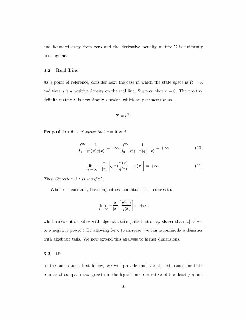
6.2 Real Line
As a point of reference, consider next the case in which the state space is Ω = R
and thus q is a positive density on the real line. Suppose that π = 0. The positive
definite matrix Σ is now simply a scalar, which we parameterize as
Σ = ς2.
Proposition 6.1. Suppose that π = 0 and
∫ ∞
0
1ς2(x)q(x)
= +∞,
∫ ∞
0
1ς2(−x)q(−x) = +∞ (10)
lim|x|→∞
− x
|x|[ς(x)
q′(x)q(x)
+ ς ′(x)]
= +∞. (11)
Then Criterion 3.1 is satisfied.
When ς is constant, the compactness condition (11) reduces to:
lim|x|→∞
− x
|x|[q′(x)q(x)
]= +∞,
which rules out densities with algebraic tails (tails that decay slower than |x| raised
to a negative power.) By allowing for ς to increase, we can accommodate densities
with algebraic tails. We now extend this analysis to higher dimensions.
6.3 Rn
In the subsections that follow, we will provide multivariate extensions for both
sources of compactness: growth in the logarithmic derivative of the density q and
16
growth in the derivative penalty Σ. For simplicity, we will concentrate in the case
where the state space is all of Rn.
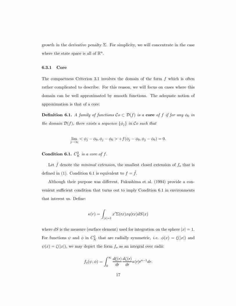
6.3.1 Core
The compactness Criterion 3.1 involves the domain of the form f which is often
rather complicated to describe. For this reason, we will focus on cases where this
domain can be well approximated by smooth functions. The adequate notion of
approximation is that of a core:
Definition 6.1. A family of functions Co ⊂ D(f) is a core of f if for any φ0 in
the domain D(f), there exists a sequence {φj} in Co such that
limj→∞
< φj − φ0, φj − φ0 > +f(φj − φ0, φj − φ0) = 0.
Condition 6.1. C2K is a core of f .
Let f denote the minimal extension, the smallest closed extension of fo that is
defined in (1). Condition 6.1 is equivalent to f = f .
Although their purpose was different, Fukushima et al. (1994) provide a con-
venient sufficient condition that turns out to imply Condition 6.1 in environments
that interest us. Define:
κ(r) =∫|x|=1
x′Σ(rx)xq(rx)dS(x)
where dS is the measure (surface element) used for integration on the sphere |x| = 1.
For functions ψ and φ in C2K that are radially symmetric, i.e. φ(x) = ξ(|x|) and
ψ(x) = ζ(|x|), we may depict the form fo as an integral over radii:
fo(ψ, φ) =∫ ∞
0
dξ(r)dr
dζ(r)dr
κ(r)rn−1dr.
17

Proposition 6.2. When π = 0, condition 6.1 is implied by:
∫ ∞
1κ(r)−1r1−ndr = ∞. (12)
.
Restriction (12) implies the scalar restriction (10) of Proposition 6.1. This follows
since for any non-negative reals r1 and r2,
min{
1r1,
1r2
}≥ 1
r1 + r2.
Notice that (12) is a joint restriction on Σ and q. We may relate this condition
to the moments of q and the growth of Σ using the inequality:
+∞ =(∫ ∞
1
1rdr
)2
≤∫ ∞
1κ(r)−1r1−ndr
∫ ∞
1κ(r)rn−3dr.
Thus a sufficient condition for (12) is that
∫ ∞
1
κ(r)r2
rn−1dr <∞. (13)
This latter inequality displays a tradeoff between growth in the penalization
matrix and moments of the distribution. Define
ς2(r) = sup|x|=1
x′Σ(rx)x,
and
�(r) =∫|x|=1
q(rx)dS(x).
18
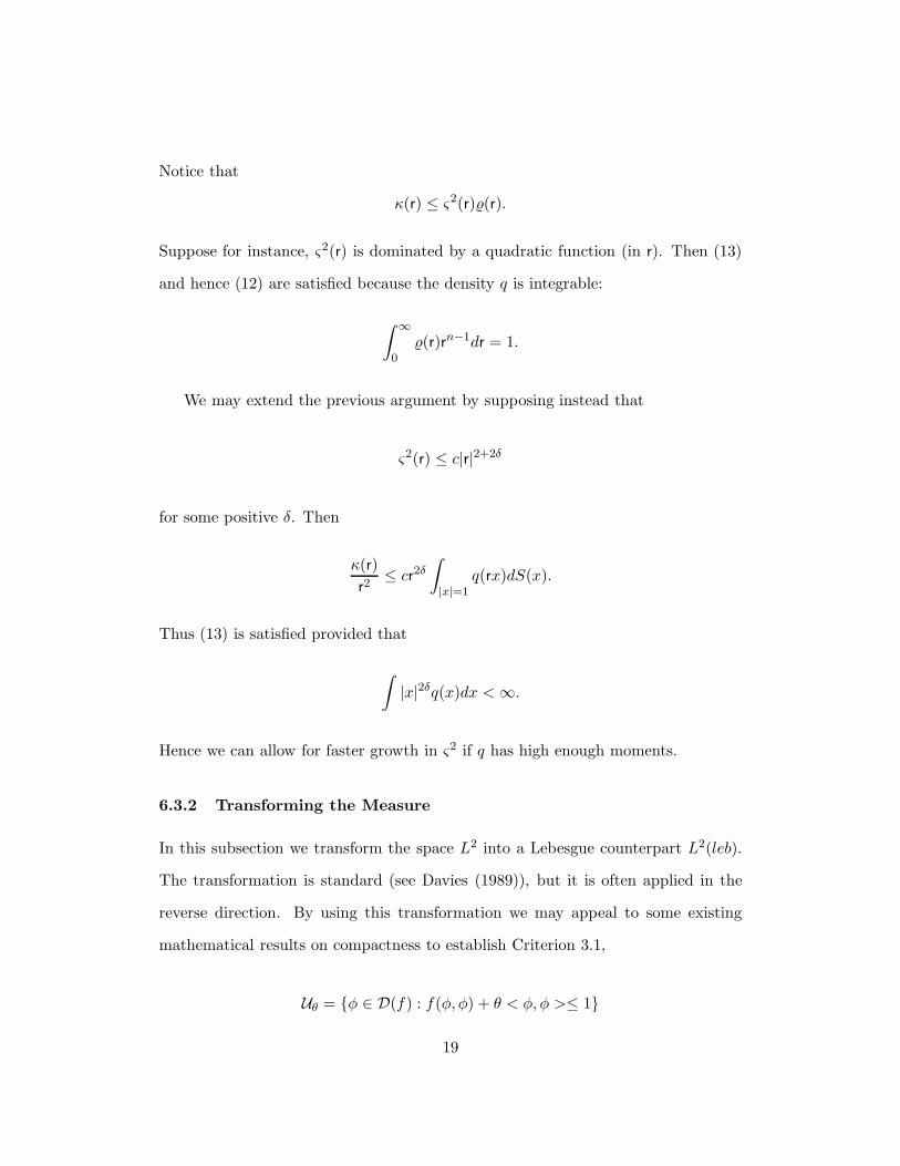
Notice that
κ(r) ≤ ς2(r)�(r).
Suppose for instance, ς2(r) is dominated by a quadratic function (in r). Then (13)
and hence (12) are satisfied because the density q is integrable:
∫ ∞
0�(r)rn−1dr = 1.
We may extend the previous argument by supposing instead that
ς2(r) ≤ c|r|2+2δ
for some positive δ. Then
κ(r)r2
≤ cr2δ
∫|x|=1
q(rx)dS(x).
Thus (13) is satisfied provided that
∫|x|2δq(x)dx <∞.
Hence we can allow for faster growth in ς2 if q has high enough moments.
6.3.2 Transforming the Measure
In this subsection we transform the space L2 into a Lebesgue counterpart L2(leb).
The transformation is standard (see Davies (1989)), but it is often applied in the
reverse direction. By using this transformation we may appeal to some existing
mathematical results on compactness to establish Criterion 3.1,
Uθ = {φ ∈ D(f) : f(φ, φ) + θ < φ, φ >≤ 1}
19
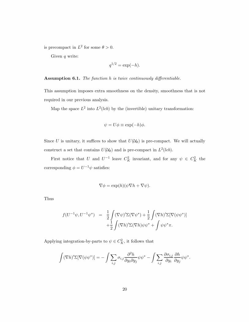
is precompact in L2 for some θ > 0.
Given q write:
q1/2 = exp(−h).
Assumption 6.1. The function h is twice continuously differentiable.
This assumption imposes extra smoothness on the density, smoothness that is not
required in our previous analysis.
Map the space L2 into L2(leb) by the (invertible) unitary transformation:
ψ = Uφ ≡ exp(−h)φ.
Since U is unitary, it suffices to show that U(Uθ) is pre-compact. We will actually
construct a set that contains U(Uθ) and is pre-compact in L2(leb).
First notice that U and U−1 leave C2K invariant, and for any ψ ∈ C2
K the
corresponding φ = U−1ψ satisfies:
∇φ = exp(h)(ψ∇h + ∇ψ).
Thus
f(U−1ψ,U−1ψ∗) =12
∫(∇ψ)′Σ(∇ψ∗) +
12
∫(∇h)′Σ[∇(ψψ∗)]
+12
∫(∇h)′Σ(∇h)ψψ∗ +
∫ψψ∗π.
Applying integration-by-parts to ψ ∈ C2K , it follows that
∫(∇h)′Σ[∇(ψψ∗)] = −
∫ ∑i,j
σi,j∂2h
∂yi∂yjψψ∗ −
∫ ∑i,j
∂σi,j
∂yi
∂h
∂yjψψ∗.
20

Therefore,
f(U−1ψ,U−1ψ∗) =12
∫(∇ψ)′Σ(∇ψ∗) +
12
∫V ψψ∗ (14)
where the potential function V is given by:
V = −∑i,j
σi,j∂2h
∂yi∂yj−
∑i,j
∂σi,j
∂yi
∂h
∂yj+ (∇h)′Σ(∇h) + 2π. (15)
Proposition 6.3. Suppose that C2K is a core for f , ψ = Uφ for some φ ∈ H and
V is bounded from below. Then ψ is weakly differentiable,
∇ψ = exp(−h)(−φ∇h+ ∇φ)
and12
∫(∇φ)′Σ∇φq +
∫φ2πq =
12
∫(∇ψ)′Σ(∇ψ) +
12
∫V ψ2. (16)
A consequence of this proposition is that
Vθ = {ψ ∈ L2(leb) :∫ (
θ +12V
)ψ2 +
12
∫(∇ψ)′Σ(∇ψ) ≤ 1} ⊃ U(Uθ),
and it thus suffices to show that Vθ is precompact in L2(leb) for some θ > 0.
We consider two methods for establishing that this property is satisfied. We first
focus on the behavior of the potential V used in the quadratic form:∫
(θ + 12V )ψ2,
and then we study extensions that exploit growth in the derivative penalty matrix
Σ used in the quadratic form:∫
(∇ψ)′Σ(∇ψ).
6.3.3 Divergent Potential
In this section, we use the tail behavior of the potential V . To simplify the treatment
of the term∫(∇ψ)′Σ(∇ψ) in the definition of Vθ we impose:
21
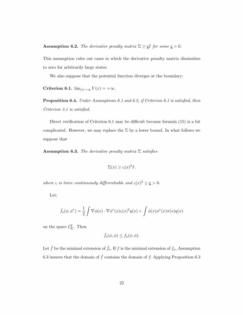
Assumption 6.2. The derivative penalty matrix Σ ≥ cI for some c > 0.
This assumption rules out cases in which the derivative penalty matrix diminishes
to zero for arbitrarily large states.
We also suppose that the potential function diverges at the boundary:
Criterion 6.1. lim|x|→∞ V (x) = +∞.
Proposition 6.4. Under Assumptions 6.1 and 6.2, if Criterion 6.1 is satisfied, then
Criterion 3.1 is satisfied.
Direct verification of Criterion 6.1 may be difficult because formula (15) is a bit
complicated. However, we may replace the Σ by a lower bound. In what follows we
suppose that
Assumption 6.3. The derivative penalty matrix Σ satisfies
Σ(x) ≥ ς(x)2I.
where ς is twice continuously differentiable and ς(x)2 ≥ c > 0.
Let:
fo(φ, φ∗) =12
∫∇φ(x) · ∇φ∗(x)ς(x)2q(x) +
∫φ(x)φ∗(x)π(x)q(x)
on the space C2K . Then
fo(φ, φ) ≤ fo(φ, φ).
Let f be the minimal extension of fo. If f is the minimal extension of fo, Assumption
6.3 insures that the domain of f contains the domain of f. Applying Proposition 6.3
22
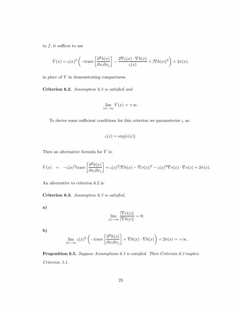
to f , it suffices to use
V (x) = ς(x)2(−trace
[∂2h(x)∂xi∂xj
]− 2∇ς(x) · ∇h(x)
ς(x)+ |∇h(x)|2
)+ 2π(x).
in place of V in demonstrating compactness.
Criterion 6.2. Assumption 6.3 is satisfied and
lim|x|→∞
V (x) = +∞.
To derive some sufficient conditions for this criterion we parameterize ς as:
ς(x) = exp[v(x)].
Then an alternative formula for V is:
V (x) = −ς(x)2trace[∂2h(x)∂xi∂xj
]+ ς(x)2|∇h(x) −∇v(x)|2 − ς(x)2∇v(x) · ∇v(x) + 2π(x).
An alternative to criterion 6.2 is:
Criterion 6.3. Assumption 6.3 is satisfied,
a)
lim|x|→∞
|∇v(x)||∇h(x)| = 0;
b)
lim|x|→∞
ς(x)2(−trace
[∂2h(x)∂xi∂xj
]+ ∇h(x) · ∇h(x)
)+ 2π(x) = +∞.
Proposition 6.5. Suppose Assumptions 6.1 is satisfied. Then Criterion 6.3 implies
Criterion 3.1.
23
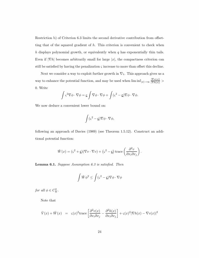
Restriction b) of Criterion 6.3 limits the second derivative contribution from offset-
ting that of the squared gradient of h. This criterion is convenient to check when
h displays polynomial growth, or equivalently when q has exponentially thin tails.
Even if |∇h| becomes arbitrarily small for large |x|, the compactness criterion can
still be satisfied by having the penalization ς increase to more than offset this decline.
Next we consider a way to exploit further growth in ∇ς. This approach gives us a
way to enhance the potential function, and may be used when lim inf |x|→∞|∇v(x)||∇h(x)| >
0. Write ∫ς2∇φ · ∇φ = c
∫∇φ · ∇φ+
∫(ς2 − c)∇φ · ∇φ.
We now deduce a convenient lower bound on:
∫(ς2 − c)∇φ · ∇φ,
following an approach of Davies (1989) (see Theorem 1.5.12). Construct an addi-
tional potential function:
W (x) = (ς2 + c)(∇v · ∇v) +(ς2 − c
)trace
(∂2v
∂xi∂xj
).
Lemma 6.1. Suppose Assumption 6.3 is satisfied. Then
∫Wφ2 ≤
∫(ς2 − c)∇φ · ∇φ
for all φ ∈ C2K .
Note that
V (x) + W (x) = ς(x)2trace[∂2v(x)∂xi∂xj
− ∂2h(x)∂xi∂xj
]+ ς(x)2|∇h(x) −∇v(x)|2
24
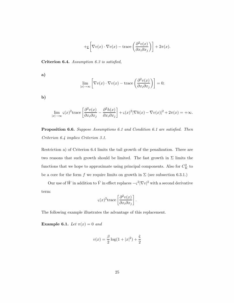
+c[∇v(x) · ∇v(x) − trace
(∂2v(x)∂xi∂xj
)]+ 2π(x).
Criterion 6.4. Assumption 6.3 is satisfied,
a)
lim|x|→∞
[∇v(x) · ∇v(x) − trace
(∂2v(x)∂xi∂xj
)]= 0;
b)
lim|x|→∞
ς(x)2trace[∂2v(x)∂xi∂xj
− ∂2h(x)∂xi∂xj
]+ ς(x)2|∇h(x)−∇v(x)|2 + 2π(x) = +∞.
Proposition 6.6. Suppose Assumptions 6.1 and Condition 6.1 are satisfied. Then
Criterion 6.4 implies Criterion 3.1.
Restriction a) of Criterion 6.4 limits the tail growth of the penalization. There are
two reasons that such growth should be limited. The fast growth in Σ limits the
functions that we hope to approximate using principal components. Also for C2K to
be a core for the form f we require limits on growth in Σ (see subsection 6.3.1.)
Our use of W in addition to V in effect replaces −ς2|∇v|2 with a second derivative
term:
ς(x)2trace[∂2v(x)∂xi∂xj
].
The following example illustrates the advantage of this replacement.
Example 6.1. Let π(x) = 0 and
v(x) =β
2log(1 + |x|2) +
c
2
25

where c = log c. Thus ς grows like |x|β in the tails. Simple calculations result in
−∇v(x) · ∇v(x) = −β2 |x|2(1 + |x|2)2 ,
and
trace[∂2v(x)∂xi∂xj
]= β
[n+ (n− 2)|x|2
(1 + |x|2)2].
Notice that both terms converge to zero as |x| gets large, but that the squared gradient
scaled by ς2 becomes arbitrarily large when β > 1. The first term is always negative,
but the second one is nonnegative provided that n ≥ 2. Even when n = 1 the second
term is larger than the first provided that β > 1.8 This example illustrates when
Criterion 6.4 is preferred to Criterion 6.3. The distinction can be important when
densities have algebraic tails.
We conclude this section by summarizing our findings so far. We provided two
criteria for constructing penalization functions that support principal component
approximation. The first one, Criterion 6.3 gives the most flexibility; but it is appli-
cable for data densities that have relatively thin tails. The second one, Criterion 6.4,
allows for densities with algebraic tails but requires that the penalization be more
severe in the extremes to compensate for the tail thickness. Making the penalization
more potent limits the class of functions that are approximated. Moreover, when
the penalization is too extreme, we encounter an additional approximation problem:
the family of functions C2K ceases to be a core for the form used in the principal
component extraction.
The next section considers refinements of results in this section, but for a limited
class of densities. These results in effect illustrate formally and in a more precise
way how the quality of approximation is altered by the tail behavior of the density8We have previously established an alternative compactness criterion for n = 1 that does not
involve second derivatives that may be preferred to Criterion 6.4.
26
and the penalization.
7 Illustration and Refinement
The optimization problem 3.1 uses a form built with a penalization matrix Σ scaled
by a density q. The density also defines the underlying sense of approximation. For
a given density, increasing the penalization effectively limits the class of functions
that can be approximated. This should result in a corresponding accuracy gain.
That is, for a fixed finite number of principal components we should be able to
approximate better a smaller class of functions. Changing the density q changes the
norm of the space L2. In particular, when we make the tail of the density thicker,
the sense of approximation becomes more stringent. While it is too ambitious to
establish a full array of exact results, we will be able to illustrate these effects for
some examples.
In this section we first specialize the general compactness criteria of section 6 to
the case of a radially symmetric density and penalization function. We study four
parameterized classes of examples, two with densities that have exponential tails and
two with densities that have thicker algebraic tails. We first derive bounds on the
parameters that guarantee that we can apply radial counterparts to our compactness
criteria 6.3 and 6.4 above. We then present bounds on the rate of divergence of the
eigenvalues δj associated with the principal component extraction. Recall that these
eigenvalues measure the smoothness of the principal components and are related to
the bounds, λj, on the least squares approximation error second moments via the
formula:
λj =1
1 + θδj. (17)
Thus by bounding the rate of divergence of the eigenvalues, we bound the rate of
27

convergence of the approximation errors.
All of our examples presume that π is zero. This closes down one of the channels
for a divergent potential and instead features the role of q and Σ.
7.1 Compactness under Radial Symmetry
Prior to our analysis of some examples, we consider the specialization of our com-
pactness criteria when radial symmetry is imposed. Recall that q(x) = exp[−2h(x)]
and Σ(x) ≥ exp[2v(x)]. Suppose that
h(x) = η(|x|)v(x) = ν(|x|),
then
∇h(x) = x|x|η
′(|x|), trace[
∂2h(x)∂x∂x′
]= (n−1)
|x| η′(|x|) + η′′(|x|),
where when necessary we use the weak notion of a derivative. The radial counterpart
to compactness Criterion 6.3 is
Criterion 7.1. Assumption 6.3 is satisfied,
a)
limr→∞
ν ′
η′= 0;
b)
limr→∞ exp(2ν)
[−(n− 1)
rη′ − η′′ + η′2
]= +∞.
Similarly, the radial counterpart to compactness Criterion 6.4 is:
Criterion 7.2. Assumption 6.3 is satisfied,
28

a)
limr→∞−(n− 1)
rν ′ − ν ′′ + (ν ′)2 = 0;
b)
limr→∞ exp(2ν)
[ν ′′ − η′′ +
(n− 1)r
(ν ′ − η′) + (η′ − ν ′)2]
= +∞
We will apply these criteria in the examples that follow.
7.2 Four Examples
Example 7.1. (Exponential Decay I) Suppose that
η(r) = c1(1 + r2)ξ2 + c2,
exp[2ν(r)] = c(1 + r2)β.
For this example we use compactness Criterion 7.1. A simple calculation shows
that part a) is satisfied and that part b) is dominated by exp(2ν)(η′)2. The resulting
potential function behaves like
c(c1)2ξ2(1 + r2)ω
for large r where
ω = β + ξ − 1.
Compactness requires that ω exceeds zero and thus depends on the sum of β and ξ.
This dependence depicts a simple tradeoff between the tail behavior of the density
and the potency of the penalization. In particular, as long as ξ > 1, we still have
compactness even when the penalization matrix Σ is the identity matrix.
Our second example includes a limiting case of Example 7.1 in which ξ = 1. If
29
β were also set to zero, principal components would fail to exist because we would
be attempting to approximate a class of functions that is too large. We shrink the
set by including a logarithmic specification of ς.
Example 7.2. (Exponential Decay II) Suppose that η is the same as in Example
7.1 but that we consider a less potent penalty function:
η(r) = c1(1 + r2)ξ2 + c2,
exp[2ν(r)] = c[log(1 + r2)]τ + c
where ξ ≥ 1 and τ ≥ 0.
As in Example 7.1, we apply Criterion 7.1. In this case, however, the potential
function behaves like:
c(c1ξ)2[log(1 + r2)]τ (1 + r2)ξ−1
for large r. Notice that the potential function diverges even when ξ = 1 provided
that τ > 0.
Our next example considers densities with algebraic tails.
Example 7.3. (Algebraic Decay I)9 Suppose
η(r) =γ
2log(1 + r2) + c∗.
where γ > n/2 for the resulting q to be integrable. Consistent with our previous
example and Example 6.1, let
ν(r) =β
2log(1 + r2) +
c
2
where c = log c. We now restrict β > 1.9Pang (1996) gives an extended analysis of an example similar to this.
30
In this case we use compactness Criterion 7.2. Simple calculations result in
(η′ − ν ′)2 = (β − γ)2r2
(1 + r2)2(n− 1)
r(ν ′ − η′) = (n− 1)(β − γ)
11 + r2
ν ′′ − η′′ = (β − γ)1 − r2
(1 + r2)2
Provided that γ−β > n− 2 the potential function Criterion 7.2 is guaranteed to be
positive and to diverge for large r. Moreover, Proposition 6.2 guarantees that C2K is
a form core when Σ = ς2I.10
For this example, γ has to be large relative to β to ensure that the potential
function has the correct sign in the tails and that C2K is a form core. On the other
hand, it does not influence the rate at with the potential function diverges. Instead
the potential function behaves like
[(β − γ)2 + (β − γ)(n − 2)](1 + r2)ω
for ω = β − 1. The value of γ only alters the scaling factor.
The following example studies a limiting case of the algebraic tail, but with a
weak penalty. Thus we set β = 1, a value not allowed in our previous investigation,
but we include a more modest penalty term.
Example 7.4. ( Algebraic Decay II) As in our previous example, suppose
η(r) =γ
2log(1 + r2) + c∗.
10By optimizing over the choice of the potential function, this inequality can be improved to be:γ − β > n
2− 1 and Proposition 6.2 may still be used to establish that C2
K is a form core.
31
where γ > n/2, and let
exp[2ν(r)] = c(1 + r2)(1 + [log(1 + r2)])τ
for τ > 0.
In this example it can be shown that the potential function of Criterion 7.2
behaves like scale multiple of (1 + [log(1 + r2)])τ for large r. Consistent with our
previous example, we restrict γ > n − 1 to ensure that the potential function is
positive and that C2K is a core for the form.
The four examples illustrate the application of the compactness criteria. When
the potential functions diverge more rapidly, approximation becomes easier in the
sense that we obtain sharper bounds on the decay rate of the eigenvalues. We show
this formally in the next subsections.
7.3 Some benchmark results on eigenvalue decay
Consider two forms f1 and f2 with common cores such that f2 ≥ f1 on a core for
the form f2. Then the jth eigenvalue of the form f2 is greater than or equal to the
jth eigenvalue of the form f1 (e.g. see Edmunds and Evans (1987), Lemma 2.3).
This gives us an operational way to use eigenvalue divergence for special forms to
bound the eigenvalue divergence of the forms of interest. For this reason we start by
deriving sharp bounds on parameterized versions of two forms studied previously in
the literature:
fw(φ,ψ) =∫φψw +
∫∇φ∇ψ,
and
fdw(φ,ψ) =
∫φψw +
∫∇φ∇ψw
32
defined on the appropriately defined subspaces of L2(leb). We will apply the follow-
ing three results in our subsequent analysis. Our first result gives a characterization
of the eigenvalues of a parameterization of fw.
Claim 7.1. Let w(x) = (1 + |x|2)ω for some ω > 1/2. Then the jth eigenvalue of
fw satisfies:11
δj ∼ (j + 1)2ω
n(1+ω) .
The second two results consider two alternative parameterizations of the form
fdw.
Claim 7.2. Let w(x) = (1 + |x|2)ω for ω > 0. The eigenvalues δj of fdw satisfy:
• If ω > 1, then δj ∼ (j + 1)2n .
• If 0 < ω < 1, then δj ∼ (j + 1)2ωn .
• If ω = 1, then δj ∼(
j+1log(j+1)
) 2n .
Claim 7.3. Let w(x) = [1 + log(1 + |x|2)]τ for τ > 0. Then the eigenvalues δj of
fdw satisfy
δj ∼ [log(j + 1)]τ .
Notice that in comparing the results in Claims 7.2 and 7.3, we see that weaker
penalties slow the decay rate in the eigenvalues.
In the remainder of this section we shall apply these claims to obtain bounds on
the eigenvalues of the form f .11The notation δj ∼ aj means that there are two positive finite constants c� and cu such that
c�aj ≤ δj ≤ cuaj for all j.
33
7.4 Lower bounds
We now reconsider the four examples described previously using bounding argu-
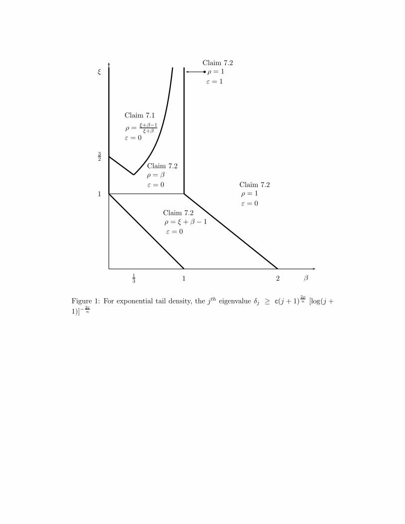
ments. Consider first Example 7.1. In this example we use either ω = β + ξ − 1 in
conjunction with Claim 7.1 or ω = min{β + ξ− 1, β} in conjunction with Claim 7.2
to obtain a lower bound on the divergence rate of the eigenvalues depending upon
which claim gives the best results. The outcome of this comparison is depicted in
Figure 1.
This figure depicts a tradeoff between the thinness of tail density as captured
by the parameter ξ and the strictness of the penalty β. In the far right region
the divergence rate matches that when the state space is compact with minimum
smooth boundary and the density is bounded and bounded away from zero (see e.g.
Edmunds and Evans (1987), Theorem V.6.5). When β = 0, we fail to obtain a
bound on the eigenvalue divergence when 1 < ξ < 3/2 even though we know that
the potential function diverges, albeit at a slow rate. This is evidently a case in
which approximation is particularly difficult and eigenvalue decay is slow.
Consider Example 7.2. For ξ ≥ 3/2 we can bound the eigenvalue decay just as
in Example 7.1 with β = 0 by applying Claim 7.1. For 1 ≤ ξ < 3/2, we use Claim
7.3 to bound the eigenvalues. Combining these results gives:
• (Claim 7.3) If 1 ≤ ξ < 3/2, then δj ≥ c[log(j + 1)]τ
• (Claim 7.1) If ξ ≥ 3/2, then δj ≥ c(j + 1)2(ξ−1)
nξ
The first region for ξ is of particular interest to us. In Example 7.1, when β = 0
we ruled out ξ = 1 to achieve existence, and we eliminated entirely this first region
for ξ to obtain bounds on the eigenvalues. We include this region by imposing a
weak penalty, but obtaining a correspondingly weak bound on the eigenvalue decay.
34
Consider next Example 7.3. In this case the eigenvalue decay bounds are dictated
by the magnitude of β. Applying Claim 7.2 with ω = β − 1, we obtain:12
• If β > 2 then δj ≥ c(j + 1)2n .
• If β = 2 then δj ≥ c(j + 1)2n [log(j + 1)]−
2n .
• If 1 < β < 2, then δj ≥ c(j + 1)2(β−1)
n .
The value of γ limits how large β can be because of the form core restriction.
Finally, the eigenvalue decay rate for Example 7.4 is given by Claim 7.3. The
rate becomes arbitrarily slow as τ declines to zero.
7.5 Upper bounds
So far we have derived lower bounds on the decay of the eigenvalues of the form. As
we saw from formula (17), these lower bounds give upper bounds on the ability to
approximate with a finite number of principal components. Thus these bounds are
informative as to when approximation problems are relatively easy. Upper bounds
on the decay of the eigenvalues of the form can also be valuable. Not only do
they allow us to infer when the lower bounds are relatively sharp, they can be
used to inform as to when approximation problems are difficult. Upper bounds on
eigenvalues can be obtained by using upper bounds on forms as we now illustrate.
Consider Example 7.1 with β = 0. We have already verified that the potential
function diverges for 1 < ξ < 3/2, but we failed to give a lower bound on the
eigenvalue decay. Applying Claim 7.1 in conjunction with divergence rate of the
potential function, we obtain the upper bound:
δj ≤ c(j + 1)2(ξ−1)
n ,
12Notice that when β > 3/2, Claim 7.1 also can be applied with ω = β − 1. However, Claim 7.2provides sharper eigenvalue bounds.
35

but in this case the bound is necessarily weak. When ξ = 1 and we include the
limiting penalization given in Example 7.2, we find that
δj ≤ c[log(j + 1)]τ
and our bound is now sharp. The slow eigenvalue decay in this example implies that
the resulting approximation problem is a particularly challenging one.
8 Conclusions
In this paper we have explored how to use restrictions on three weighting func-
tions to show when there is a discrete spectral representation of semigroups for
Markov processes. We obtain these results using quadratic forms as a way to embed
the generators of the semigroups. The weighting functions have explicit interpre-
tations, and in particular one of the weighting functions is the stationary density
for the diffusion. This weighting function replaces the usual specification of drift
of the Markov diffusion. Specifically, the drift can be constructed as function of
two weighting functions. In this sense our prior restriction are in part restrictions
on the long run behavior of the dynamic system. Our results complement those of
related literature that features drift conditions instead of weighting functions. See,
for instance, Kontoyiannis and Meyn (2003).
We established bounds on the behavior of eigenvalues by applying the weighted
compact embedding approach, where the weights are related to the tail behavior of
(Σ, q, π). There is an alternative method to establish bounds on eigenvalue decay
rate by using functional inequalities (such as the log-Sobolev and the super-Poincare
inequalities); see e.g. Wang (2000). Our approach is germane for building Markov
diffusion semigroups from a quadratic form characterized by (Σ, q, π). In appli-
36
cations, it is sometimes advantageous to restrict the Markov process through the
behavior of an implied stationary density q dictated by long-run or low frequency be-
havior. (For example, see Chen et al. (2007) and Hansen and Scheinkman (2007).)
Our results are easily applicable to verify the existence of discrete spectrum and
eigenvalue decay bounds in these kinds of applications.
Applications of these semigroup methods often explore a parameterized family of
semigroups. Appropriately defined derivatives of these semigroups are also targets
of interest. See for instance Kontoyiannis and Meyn (2003) in their study of large
deviations using the Gartner-Ellis theorem or Hansen (2007) is his use of these
methods to study risk prices and local sensitivity of valuation in economic dynamics.
These and other applications suggest that a further investigation of parameterized
families of semigroups would be fruitful.
37

A Proofs
To show that the form f is a closed extension of fo, we verify that H is a Hilbert
space.
Proposition A.1. H is a Hilbert space.
Proof of Proposition A.1. Let Λ be the symmetric square root of the penalty matrix
Σ. If {φj} is a Cauchy sequence in H, then {φj} and the entries of {Λ∇φj} form
Cauchy sequences in L2. Denote the limits in L2 as
φ = limj→∞
φj
v = limj→∞
Λ∇φj .
For each u ∈ C1K we know that:
∫φj∂u
∂x= −
∫(∇φj)u,
where ∂u∂x is the partial derivative of u with respect to x. Since Σ is positive definite
and continuous on any compact subset of Ω and u vanishes outside any such set, it
follows that ∫φ∂u
∂x= −
∫(Λ−1v)u.
Hence φ ∈ H with ∇φ = Λ−1v. Moreover, φn → φ in H.
Proof of Claim 3.1. Let φ∗ solve Problem 3.1. Then for each ψ ∈ H and r ∈ R+
small
< φ∗ + rψ, φ∗ + rψ >
θ < φ∗ + rψ, φ∗ + rψ > +f(φ∗ + rψ, φ∗ + rψ)≤ λ
.=< φ∗, φ∗ >
θ < φ∗, φ∗ > +f(φ∗, φ∗).
38
That is:
2r < φ∗, ψ > +r2 < ψ,ψ >≤ λ[2rθ < φ∗, ψ > +r2θ < ψ,ψ > +2rf(φ∗, ψ)+r2f(ψ,ψ)].
Dividing by 2r and taking limr→0
< φ∗, ψ >≤ λ[θ < φ∗, ψ > +f(φ∗, ψ)].
Since we could use also −ψ,
< φ∗, ψ >= λ[< φ∗, ψ > +f(φ∗, ψ)]
for each ψ ∈ H.
Proof of Proposition 6.1. Hansen et al. (1998) consider densities from stationary
scalar diffusions, whose boundaries are not attracting. This proposition gives an
equivalent statement of their compactness condition, written in terms of the sta-
tionary density. The scalar diffusion coefficient in their analysis is ς2.
We now present a criteria for Condition 6.1 to hold. This result is due essentially
to Azencott (1974) and Davies (1985).
Proposition A.2. Consider a form fo that satisfies the Beurling-Deny Criterion
5.1 and π = 0. Let f denote the minimal extension of fo with domain D(f). Suppose
that 1 ∈ D(f) and f(1, φ) = 0 for all φ ∈ D(f). Then f = f .
Proof of Proposition A.2. As explained in Sections 4 and 5, associated with the
forms f and f we may construct operators F and F and resolvents G and G.
Integration by parts can be used to show that the operators F and F are extensions
39
of the differential operator
Lφ = −1q
∑i,j
∂
∂x i
(qσij
∂φ
∂xj
),
defined on C2K . The form f and hence the form f satisfies the Beurling-Deny Cri-
terion 5.1 (Davies (1989) Theorem 1.3.5). Hence as stated in Davies (1985) the
operators F and F can be extended to subspaces of L1. Similarly the resolvents
G and G can be extended to L1. We will denote the extended operators as F 1,
F 1, G1, and G1. Since q is integrable, L2 convergence implies L1 convergence and
consequently F and F are restrictions of F 1 and F 1, respectively. Similarly for the
resolvent operators.
If f(1, φ) = 0 for all φ ∈ D(f) then F1 = 0 and G1 = 1. Consequently G11 = 1.
It follows from Theorem 2.2 in Davies (1985) that C2K is a core for F 1, in the sense
that F 1 is the closure in L1 of L.13 Hence C2K is a core for F 2, and thus a core for
f or, equivalently, f and f coincide.
Proof of Proposition 6.2. Since f is the minimal closed extension, it has C2K as
its core. When this condition is met, a sequence of functions φj in C2K can be
constructed that converge to 1 in L2 and f(φj , φj) converges to zero. See Fukushima
et al. (1994) Theorem 1.6.6 and Theorem 1.6.7. An approximating sequence of
functions with compact support is supplied by Fukushima et al. (1994) in the proof
of Theorem 1.6.7. This sequence can be smoothed using a suitable regularization
to produce a corresponding approximating sequence in C2K . Thus the unit function
is in the domain of f and f(1, φ) = 0 for φ ∈ C2K and hence for φ ∈ D(f). As we
established above, this is sufficient for Condition 6.1.
13Davies (1985) assumes that the coefficients of L are C∞. However the proof holds for C2
coefficients since elliptic regularity holds even when the coefficients are only Lipschitz (see Theorem6.3 of Agmon (1965))
40

Proof of Proposition 6.3. Since V is bounded from below, we may choose a θ > 0
such that V + θ is nonnegative. Construct the space:
H.= {ψ ∈ L2(leb) :
∫(V + θ)(ψ)2 <∞, there exists g measurable, with
∫g′Σg <∞,
and∫ψ∇ϕ = −
∫gϕ, for all ψ ∈ C1
K}.
As in the proof of Proposition A.1, it follows that H is a Hilbert space with inner
product: ∫(V + θ + 1)ψψ +
∫(∇ψ)′Σ(∇ψ).
We show that UH ⊂ H.
Since C2K is a core for f , there exists a sequence {φj : j = 1, 2, ...} in C2
K that
converges to φ in the Hilbert space norm of H. Hence this sequence is Cauchy in
that norm. Writing ψj = Uφj and applying equation (14) we obtain:
∫(φj − φ�)2(1 + θ)q +
∫(∇φj −∇φ�)′Σ(∇φj −∇φ�)q
=∫
(V + θ + 1)(ψj − ψ�)2 +∫
(∇ψj −∇ψ�)′Σ(∇ψj −∇ψ�).
Thus {ψj : j = 1, 2, ...} is Cauchy in the Hilbert space norm of H and the limit point
ψ must satisfy ψ = Uφ. Notice that∫V (ψ)2 +
∫(∇ψ)′Σ(∇ψ) equals H squared
norm minus θ + 1 times the L2(Q) squared norm. Thus,
∫V (ψ)2 +
∫(∇ψ)′Σ(∇ψ) = lim
j→∞
∫(∇ψj)′Σ(∇ψj)q
= limj→∞
(∇φj)′Σ(∇φj)q
=∫
(∇φ)′Σ(∇φ)q.
This proves (16).
41
For a given ψ = Uφ our candidate for the weak derivative is,
g.= exp(−h)(−φ∇h + ∇φ).
To verify that g is indeed the weak derivative, we must show that for any ϕ ∈ C1K
∫ψ∇ϕ = −
∫gϕ, (18)
and ∫g′Σg <∞. (19)
We check relation (18) by applying integration by parts,
−∫
∇ψϕ = −∫
[exp(−h)(−φ∇h+ ∇φ)]ϕ = −∫
∇φ exp(−h)ϕ +∫
exp(−h)ϕφ∇h
=∫φ[exp(−h)∇ϕ −∇h exp(−h)ϕ] +
∫exp(−h)ϕφ∇h =
∫ψ∇ϕ.
Inequality (19) follows from (16).
Proof of Proposition 6.4. Since V is continuous and diverges at the boundaries, it
must be bounded from below. Also, it follows from Assumption 6.2 that
Vθ ⊂ {ψ ∈ L2(leb) : ψ has a weak derivative and∫ (θ +
12V
)(ψ)2 +
c
2
∫|∇ψ|2 ≤ 1}.
We may then apply the argument in the proof of Theorem XIII.67 of Reed and
Simon (1978) to establish that Vθ is precompact in L2(leb).
42
Proof of Lemma 6.1. Consider a positive function χ(x) = (ς(x))−1, and note that
[ς(x)2 − c
]∇χ(x) = −ς(x)∇v + c∇v(x)ς(x)
.
For φ in C2K we may apply integration by parts to show that
∫(ς2 − c)∇χ · ∇φ =
∫ [(ς2 + c
ς
)(∇v · ∇v) +
(ς2 − c
ς
)trace
(∂2v
∂xi∂xj
)]φ
=∫Wχφ
The conclusion now follows from Theorem 1.5.12 of Davies (1989). While Davies
(1989) uses test functions φ in C∞K , the same proof applies to C2
K test functions.
Finally, we consider the three results related to eigenvalue decay.
Proof of Claim 7.1. Reed and Simon (1978) (Theorem XIII.81) show that the num-
ber of eigenvalues of fw that are less than or equal to r > 0 can be bounded above
and below by scale multiples of14
∫ u
0[r − (1 + u2)ω]
n2 un−1du, with u =
(r
1ω − 1
) 12.
Since r ≥ r − (1 + u2)ω, the integral is dominated by
rn2
∫ u
0un−1du =
1n
rn2 un
Thus the integral can be dominated by a scale multiple of rn2+ n
2ω . An analogous
upper bound can be formed with an appropriate adjustment in the constant term.
14While Reed and Simon (1978) only prove this result for n ≥ 2, they argue that the resultextends to the n = 1 case.
43
Proof of Claim 7.2. Use the form fdw to construct an inner product and a corre-
sponding Hilbert space, and consider the embedding operator (identity operator)
mapping this space into L2(leb). Proposition 4.1 of Mynbaev and Otel’baev (1988)
established the exact order of the approximation numbers {aj : j ≥ 0} for this
embedding operator. The result follows by using the known relation (δj)−1/2 = aj
between the approximation numbers of an embedding operator and eigenvalues.
(See Theorem 5.10 of Edmunds and Evans (1987).)
Proof of Claim 7.3. Again we use the form fdw to construct an embedding operator
as in the previous proof. For the choice of w given in this claim, Haroske (1997)
(Proposition 4.4) established the exact order of its entropy numbers: ej ∼ [log(j +
1)]−τ2 . Entropy number ej for an operator mapping into L2(leb) is the infimum of
all ε > 0 for which there exist 2j balls in L2(leb) with radius ε which cover the image
of the operator over the unit ball implied by the form. For this problem, entropy
numbers behave like approximation numbers. For instance, inequality (3.0.9) in Carl
and Stephani (1990), page 120 states that aj ≤ 2ej , and the Theorem in Triebel
(1994) implies that ej ≤ caj for some positive number c.15 Given the essential
equivalence of the behavior of approximation numbers and entropy numbers, the
conclusion follows from the relationship (δj)−1/2 = aj mentioned above.
15The second inequality follows from part (ii) of the Theorem in Triebel (1994) by setting Triebel’sf(j) equal to the reciprocal of the entropy numbers. With this construction the inequality is animplication of Triebel’s equation (5).
44
β
ξ
1
21
32
13
ρ = 1ε = 1
Claim 7.2
ρ = ξ+β−1ξ+β
ε = 0
Claim 7.1
ρ = ξ + β − 1ε = 0
Claim 7.2
ρ = 1ε = 0
Claim 7.2ρ = β
ε = 0
Claim 7.2
Figure 1: For exponential tail density, the jth eigenvalue δj ≥ c(j + 1)2ρn [log(j +
1)]−2εn
References
Agmon, S. 1965. Lectures on Elliptic Boundary Problems. Priceton: Vos Nostrand.
Azencott, R. 1974. Behavior of Diffusion Semi-groups at Infinity. Bull. Soc. Math.
France 102:193–240.
Beurling, A. and J. Deny. 1958. Espaces de Dirichlet I, le cas Elementaire. Acta
Math. 99:203–224.
Brezis, H. 1983. Analyse Fonctionelle. Paris: Masson.
Carl, B. and I. Stephani. 1990. Entropy, Compactness and the Approximation of
Operators. Cambridge University Press.
Chen, X., L. P. Hansen, and J. Scheinkman. 2007. Principal Components and
Long Run Implications of Multivariate Diffusions. Mimeo, University of Chicago,
Princeton University and Yale University.
Davies, E. B. 1985. L1 Properties of Second Order Operators. Bulletin of the London
Mathematical Society 17:417–436.
———. 1989. Heat Kernels and Spectral Theory. Cambridge University Press.
Edmunds, D. E. and W.D. Evans. 1987. Spectral Theory and Differential Operators.
Oxford University Press.
Fukushima, M. 1971. Dirichlet Spaces and Strong Markov Processes. Transactions
of the American Mathematics Society 162:185–224.
Fukushima, M., Y. Oshima, and M. Takeda. 1994. Dirichlet Forms and Symmetric
Markov Processes. Walter de Gruyter.
Hansen, L. P. 2007. Modeling the Long Run: Valuation in Dynamic Stochastic
Economies. Mimeo, Fisher Schultz Lecture for the 2006 Meetings of the European
Econometric Society.
Hansen, L. P. and J. Scheinkman. 2007. Long Term Risk: An Operator Approach.
Mimeo, University of Chicago and Princeton University.
Hansen, L. P., J. Scheinkman, and N. Touzi. 1998. Spectral Methods for Identifying
Scalar Diffusions. Journal of Econometrics 86:1–32.
Haroske, D. 1997. Some Limiting Embeddings in Weighted Function Spaces and
Related Entropy Numbers. Forschungsergebnisse Math/Inf 97/04, Universitat
Jena, Germany.
Kontoyiannis, I. and S. P. Meyn. 2003. Spectral Theory and Limit Theorems for
Geometrically Ergodic Processes. Annals of Applied Probability 13:304–362.
Mynbaev, K. and M. Otel’baev. 1988. Weighted Functional Spaces and Differential
Operator Spectrum. Nauka.
Pang, M. M. H. 1996. L1 and L2 Properties of a Class of Singular Second Order
Elliptic Operators on RN with Measurable Coefficients. Journal of Differential
Equations 129:1–17.
Reed, M. and B. Simon. 1978. Methods of Modern Mathematical Physics IV: Anal-
ysis of Operators. Academic Press.
Triebel, H. 1994. Relations between Approximation Numbers and Entropy Numbers.
Journal of Approximation Theory 78.
Wang, F.-Y. 2000. Functional inequalities, semigroup properties and spectrum es-
timates. Infin. Dimen. Anal. Quantum Probab. Relat. Topics 3:263–295.