Spectral Approach to Quantum Percolation on the Honeycomb ...
15
Spectral Approach to Quantum Percolation on the Honeycomb Lattice Adam Cameron, Eva Kostadinova, Forrest Guyton, Constanze Liaw, Lorin Matthews, Truell Hyde Center for Astrophysics, Space Physics, and Engineering Research One Bear Place 97310, Waco, Texas, 76798-7310 USA Application to Material Science Quantum Percolation Ominous Failures Distributions Honey Comb Code 0.30% Region www.baylor.edu/CASPER Classical Percolation Classical percolation is a problem in graph theory that seeks theta(p), the probability that the origin in an infinite graph will be part of an infinite open cluster. For site percolation all bonds are considered open, and the value p is the probability of any particular vertex being open. Study into this problem has revealed that there exists a critical point; any value of p below this point will result in theta(p) = 0. Any theta(p) greater than this point will result in theta(p) > 0. The graph above represents a simulation of classical percolation in a honeycomb shaped graph. p is the probability of any vertex being open and theta(p) is percolation probability. The critical point for this lattice structure is about 0.69, as can be seen. To the right is an example of the honeycomb structure. Quantum percolation is a variation on regular percolation that attempts to take percolation and use it to model electron flow in atomic structures. Because electrons are subject to quantum effects, the more primitive classical site percolation which simply assigns vertices as open or closed is insufficient. Quantum percolation uses a Hamiltonian to represent the change in the wave over time. This method accounts for effects such as the electron being able to jump back and forth to previous sites. One effect noticed during analysis an was occasional sudden drop in the distance D. This frequently results in the function dropping almost immediately to zero. The above is the graph for 30 realizations of a the same doping (0.9%). Most of the realizations follow a similar course remaining very close to 1 during the whole run. One suddenly drops to about 0.9 and then remains steady. And, close inspection reveals that one drop to 0 almost immediately after the beginning of the simulation. The cause of these sudden drops is currently unknown. Is it a flaw in the simulation code or the mathematical method? Or, does it represent some unusual yet legitimate phenomena? In any case, finding the reason for this behavior will be key to getting good results and properly interpreting them. Since it does seem to occur less often for lower doping, the remainder of our results come from very small doping simulations and avoid this behavior. One of the challenges faced during this project was properly representing the graphene’s 2D honeycomb structure within our program. This structure proved more difficult than the 2D square or triangular structures. To the right is a diagram that gives a rough idea of how it is done. The organic honeycomb structure is broken down into a more grid like structure that can be interpreted by the computer. In our simulations, an energy must be assigned to each site. We decided to do this assignment according to a Gaussian distribution (left above). In order to account for the effect of doping in materials, we also used another distribution (right below). This distribution is a combination of a Gaussian curve centered at 0 and a delta function centered at 100. The delta portion represents the probability of a site being doped and therefore having a much higher energy and being far more difficult for an electron to jump to. For sufficient doping, electron transport will not be possible, but it is hoped that the critical point in percolation can be connected to an amount of doping that serves as a transition point between conductivity and insulation in actual materials. It has been speculated that this point might be around .3%. In the below graph, the end values of different simulations are clustered together, with two main clusters emerging. It does seems that the blue cluster consists entirely of doping values above 0.30%. The correlation is not perfect though as there are some values above 0.30% in the red cluster. Further study will be required to see if this is the desired critical point. The main application of these studies into percolation is finding a way of modeling the electron transport properties of 2D materials, such as graphene. Graphene is a recently discovered allotrope of carbon that is truly 2-dimensional. It has a honeycomb structure the same as that used in our simulations. It is hoped that graphene will demonstrate useful electronic properties, such as semi conductivity. However graphene defies the current model for electron transfer, which is based on Anderson localization. In order to take advantage of the exciting properties of graphene, a new electron transfer model will be needed. It is hoped that this work with quantum percolation and the spectral method will lead to such a model. Funding from the National Science Foundation (PHY 1414523, PHY 1740203 and PHY 1707215) and NASA (1571701) is gratefully acknowledged. Conclusions • Unexplained failures exist for doping above 0.08%. These will require further study. • 0.30% doping may be a transition point in the quantum percolation problem corresponding to a change in the electron transport properties of 2D materials
Transcript of Spectral Approach to Quantum Percolation on the Honeycomb ...
Spectral Approach to Quantum Percolation on the Honeycomb Lattice
Adam Cameron, Eva Kostadinova, Forrest Guyton, Constanze Liaw, Lorin Matthews, Truell HydeCenter for Astrophysics, Space Physics, and Engineering Research
One Bear Place 97310, Waco, Texas, 76798-7310 USA
Application to Material Science
Quantum Percolation
Ominous Failures
Distributions
Honey Comb Code
0.30% Region
b.
www.baylor.edu/CASPER
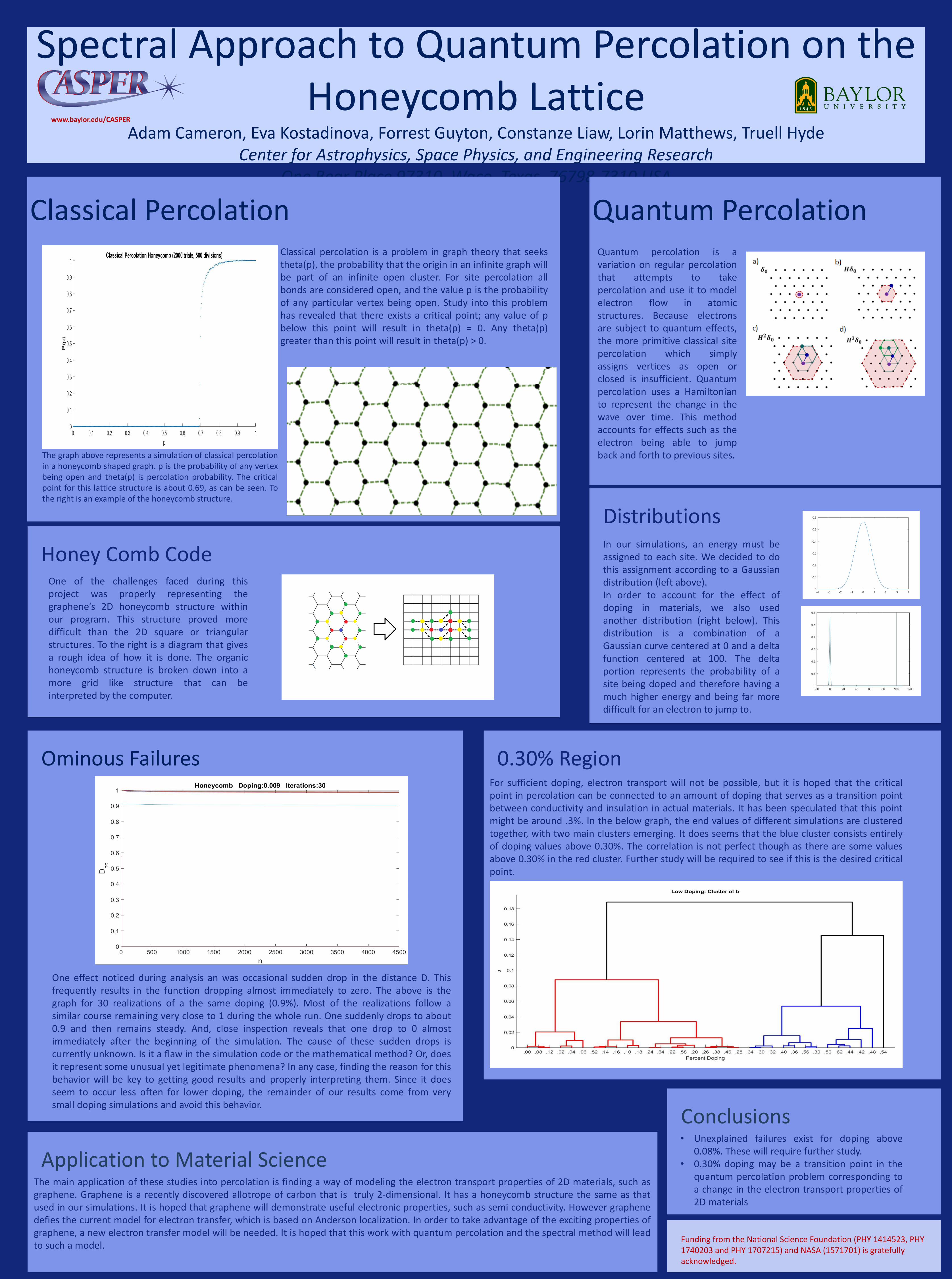
Classical PercolationClassical percolation is a problem in graph theory that seekstheta(p), the probability that the origin in an infinite graph willbe part of an infinite open cluster. For site percolation allbonds are considered open, and the value p is the probabilityof any particular vertex being open. Study into this problemhas revealed that there exists a critical point; any value of pbelow this point will result in theta(p) = 0. Any theta(p)greater than this point will result in theta(p) > 0.
The graph above represents a simulation of classical percolationin a honeycomb shaped graph. p is the probability of any vertexbeing open and theta(p) is percolation probability. The criticalpoint for this lattice structure is about 0.69, as can be seen. Tothe right is an example of the honeycomb structure.
Quantum percolation is avariation on regular percolationthat attempts to takepercolation and use it to modelelectron flow in atomicstructures. Because electronsare subject to quantum effects,the more primitive classical sitepercolation which simplyassigns vertices as open orclosed is insufficient. Quantumpercolation uses a Hamiltonianto represent the change in thewave over time. This methodaccounts for effects such as theelectron being able to jumpback and forth to previous sites.
One effect noticed during analysis an was occasional sudden drop in the distance D. Thisfrequently results in the function dropping almost immediately to zero. The above is thegraph for 30 realizations of a the same doping (0.9%). Most of the realizations follow asimilar course remaining very close to 1 during the whole run. One suddenly drops to about0.9 and then remains steady. And, close inspection reveals that one drop to 0 almostimmediately after the beginning of the simulation. The cause of these sudden drops iscurrently unknown. Is it a flaw in the simulation code or the mathematical method? Or, doesit represent some unusual yet legitimate phenomena? In any case, finding the reason for thisbehavior will be key to getting good results and properly interpreting them. Since it doesseem to occur less often for lower doping, the remainder of our results come from verysmall doping simulations and avoid this behavior.
One of the challenges faced during thisproject was properly representing thegraphene’s 2D honeycomb structure withinour program. This structure proved moredifficult than the 2D square or triangularstructures. To the right is a diagram that givesa rough idea of how it is done. The organichoneycomb structure is broken down into amore grid like structure that can beinterpreted by the computer.
In our simulations, an energy must beassigned to each site. We decided to dothis assignment according to a Gaussiandistribution (left above).In order to account for the effect ofdoping in materials, we also usedanother distribution (right below). Thisdistribution is a combination of aGaussian curve centered at 0 and a deltafunction centered at 100. The deltaportion represents the probability of asite being doped and therefore having amuch higher energy and being far moredifficult for an electron to jump to.
For sufficient doping, electron transport will not be possible, but it is hoped that the criticalpoint in percolation can be connected to an amount of doping that serves as a transition pointbetween conductivity and insulation in actual materials. It has been speculated that this pointmight be around .3%. In the below graph, the end values of different simulations are clusteredtogether, with two main clusters emerging. It does seems that the blue cluster consists entirelyof doping values above 0.30%. The correlation is not perfect though as there are some valuesabove 0.30% in the red cluster. Further study will be required to see if this is the desired criticalpoint.
The main application of these studies into percolation is finding a way of modeling the electron transport properties of 2D materials, such asgraphene. Graphene is a recently discovered allotrope of carbon that is truly 2-dimensional. It has a honeycomb structure the same as thatused in our simulations. It is hoped that graphene will demonstrate useful electronic properties, such as semi conductivity. However graphenedefies the current model for electron transfer, which is based on Anderson localization. In order to take advantage of the exciting properties ofgraphene, a new electron transfer model will be needed. It is hoped that this work with quantum percolation and the spectral method will leadto such a model.
Funding from the National Science Foundation (PHY 1414523, PHY 1740203 and PHY 1707215) and NASA (1571701) is gratefully acknowledged.
Conclusions• Unexplained failures exist for doping above
0.08%. These will require further study.• 0.30% doping may be a transition point in the
quantum percolation problem corresponding toa change in the electron transport properties of2D materials

www.baylor.edu/CASPER
Spectral Approach to Quantum
Percolation on the Honeycomb Lattice
Adam Cameron, Eva Kostadinova, Forrest Guyton, Constanze
Liaw, Lorin Matthews, Truell Hyde

www.baylor.edu/CASPEROverview
Background – Graphene, Classical Percolation, Quantum
Percolation
Method – New Honey Comb Code, Distributions,
Spectral Analysis
Results – .3% Region, Failures
Conclusions

www.baylor.edu/CASPERBackground – Graphene
Graphene is an exciting, newly
discovered 2D material.
Electrical properties defy
expectations from the current
model.
Anderson localization
New model will be required.
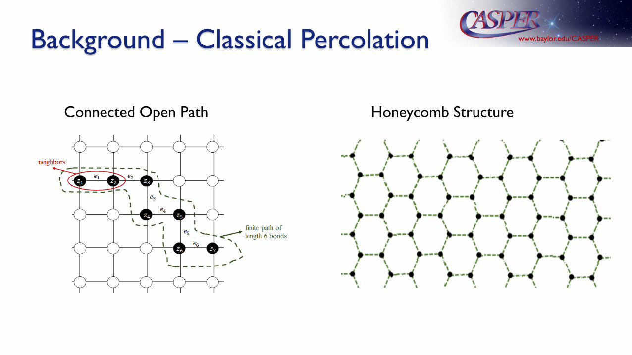
www.baylor.edu/CASPERBackground – Classical Percolation
Connected Open Path Honeycomb Structure

www.baylor.edu/CASPERBackground – Classical Percolation
Behavior of Percolation
◦ theta(0) = 0
◦ theta(1) = 1
Interest in critical point
◦ Below theta(p) = 0
◦ Above theta(p) > 0

www.baylor.edu/CASPERBackground – Quantum Percolation
Similar to classical percolation
but accounts for quantum
effects.
Uses Hamiltonian to preform
jumps.
Can jump to previous locations.

www.baylor.edu/CASPERMethod – Honeycomb Code
Hoped to improve honeycomb lattice code to run at
same speed as square and triangle lattice code
Replaced conditionals with carefully aligned vector
arithmetic. (Using Matlab’s double colon notation)
Square Triangular Honeycomb

www.baylor.edu/CASPERMethod – Honeycomb Code
Honeycomb represented
in grid form.
Dashed lines in grid
represent connections
Grid then transferred to
1D array

www.baylor.edu/CASPERMethod – Old Distributions
The old distribution used
was uniform
Gaussian would be much
more realistic

www.baylor.edu/CASPERMethod – New Distribution
Gaussian curve representing
energy variation
Delta function representing
doped particles
Doped particles are difficult to
jump to

www.baylor.edu/CASPERResults – Failures
Occasional sudden drops
Some go straight to 0
Make analysis difficult
May be caused by classical
blocks
Will require further study

www.baylor.edu/CASPERResults – 0.3% Region
Blue cluster consists
only of doping 0.3%+
Red cluster also
contains some
May be affected by
partial failures
Possibly exciting, but
requires another look

www.baylor.edu/CASPERConclusions
• Unexplained failures exist for doping above 0.08%. These
will require further study.
• 0.30% doping may be a transition point in the quantum
percolation problem corresponding to a change in the
electron transport properties of 2D materials.

www.baylor.edu/CASPERAcknowledgments
Funding from the National Science Foundation (PHY
1414523, PHY 1740203 and PHY 1707215) and NASA
(1571701) is gratefully acknowledged.