Spectral Analysis of Storm Waves using the SLEX algorithm

and the Hilbert-Huang Transform

Jose B. Hernandez Ch. ∗ J. Ortega † George H. Smith ‡

Abstract

In this work we perform a comparative study of storm wave spectra using the Hilbert-HuangTransform and the Smooth Localized complex EXponencial (SLEX) algorithm. This last algorithmdivides the data set into approximately stationary sections by detecting changes in their spectra.We compare the spectra produced by both algorithms and also look at the behaviour of theHilbert spectrum around the change points detected by SLEX. Finally, we look at large waves(higher than 6.5 m.) and their relation with the Hilbert spectrum. The data analyzed come froma North Sea storm. The results show that both methods can improve the information availablefor the understanding of time varying wave fields. The ability to produce stable, high resolutionspectra for storm conditions is of considerable interest in the design of floating offshore structures,particularly wave energy converters, which may require tuning to provide greater efficiency of waveenergy conversion.

Key words: SLEX, HHT, Hilbert spectrum, marginal Hilbert spectrum, Segmentation.

1 Introduction

Wave characteristics can change abruptly during a storm and also exhibit considerable non-lineareffects, so a first approximation for building random wave models is to assume that the sea surfaceheight, measured at a fixed point is a piecewise stationary processes, i.e. there exist instants at whichthe ’state’ of the waves changes, but between two consecutive change-points sea surface height followsa stationary process. An advantage of this approach is that classical spectral analysis can be used foreach stationary interval with the usual interpretation for the spectrum as the energy distribution ina range of frequencies. To implement this approach a method for detecting changes in the ’state’ ofthe process is required and since the spectral characteristics and covariance structure of the processwill change from one state to the next, it is reasonable to search for methods based on changes in thespectrum.

In this work we will use the SLEX (Smooth Localized complex EXponential) algorithm proposedby Ombao et al. [8] to detect changes in a storm data set that will be described in the next section.We will also use the Hilbert-Huang transform (HHT) [7] to analyze this data set and to obtain boththe Hilbert and marginal Hilbert spectra for the intervals obtained with the SLEX procedure. Thefirst method was originally employed for the analysis of non-stationary time series and the detectionof their change points while the second method is useful for the analysis of non-linear signals, using adecomposition into a series of components of different frequencies for which the Hilbert transform isused to obtain he spectrum associated to the original series. Since sea waves are often non-stationary,non-linear time series we will use both algorithms. SLEX will be used for change-point detection andboth algorithms will be used for the spectral analysis of the intervals obtained, so as to compare theresults. These algorithms are independent of each other.

∗Universidad Central de Venezuela, Caracas, Venezuela; email: jbhernandez@cantv.net†Centro de Investigacion en Matematicas (CIMAT, A.C.), Guanajuato, Gto, Mexico; email: jortega@cimat.mx‡Exeter University, Cornwall Campus, UK; email: G.H.Smith@exeter.ac.uk

1

This work is structured as follows: In section 2 we describe the data considered in this work; insection 3 a brief description of the SLEX algorithm is given. In section 4 the Hilbert-Huang transformis described, introducing first the empirical mode decomposition (EMD) and then the Hilbert spectralanalysis. Section 5 is devoted to the analysis of the storm data set using first the Slex algorithm toobtain a segmentation of the storm and then both the SLEX and HHT algorithms for the spectralanalysis. Afterwards an analysis of important events (Waves higher than 6.5 m.) is carried out. Finallythe conclusions from this work are presented.

2 Data

Data was recorded from the North Alwyn platform situated in the northern North Sea, about 100 mileseast of the Shetland Islands (60o48.5’ North and 1o44.17’ East) in a water depth of approximately 130metres. There are three Thorn EMI Infra-red wave height meters mounted on the platform and theirheights are between 25 and 35 metres above the water. The data are recorded continuously andsimultaneously at 5Hz and then divided into 20 minute records for which the summary statistics ofHs, Tp and the spectral moments are calculated. For data with Hs > 3m all the surface elevationrecords are kept. Further details are available in [11]. Only data from the North East altimeter areused here.

The present data consists of a series of records of 20 minutes duration, sampled by the altimeterat a rate of 5 Hz., The measurements were recorded between midnight on December 23rd and 9.00a.m. on December 26th 1999 and consisted of 244, 20 minute, records. Figure 1 shows the evolutionof significant wave height and peak period during the storm. This data starts at a high level with asignificant wave height of between 6.5 and 7 m and then drops down to about 3.5 m before increasingback up to around 7 m for around 20 hours. It then reduces again, before increasing to about 6.5 m,dropping to about 5 and then increasing again to around 5.5 m before finally dropping to less than3.5 m at the end of the dataset. As such this data includes two relative large increases in Hs and asection in which two peaks occur within a relatively short time period.

Figure 1: Significant wave height during the storm.

Since there were some short intervals missing in the data, it was divided into five sets that coverthe storm. In Table 1 we give a list of the five sets along with some basic characteristics of the waverecords: Significant wave height Hs, mean wave period Tm01, spectral peak period Tp and spectralbandwidth parameter ν.

3 The SLEX Algorithm

The auto-SLEX algorithm is a statistical procedure that automatically divides time series in segmentsthat are approximately stationary and automatically chooses a smoothing parameter for the estimation

2

Duration Hm Tm01 Tp νStorm1999a 8h. 40m 5.34 9.31 11.87 0.509Storm1999b 6h 3.72 8.48 11.22 0.514Storm1999c 18h 5.07 8.25 10.50 0.510Storm1999d 24h 5.87 8.99 11.70 0.492Storm1999e 24h 5.10 8.75 11.70 0.506

Table 1: Basic characteristics of the 5 data intervals.

of the spectrum that changes with time. The method is based on the SLEX (Smooth Localized complexEXponential) transform, which uses the SLEX vectors which are closely related to the classical Fouriertransform. The method is presented in [8] and we follow here their presentation. The algorithms havebeen implemented in Matlab and are available in the web-page www.stat.uiuc.edu/∼ombao.

As is well-known, Fourier functions are adequate for representing stationary random processes, sincethey are localized in frequency and the spectral properties of stationary processes are time-invariant,but they cannot represent, accurately, processes with time-evolving spectral properties. To tackle thetime localization problem, smooth compactly supported windows have been applied, but the functionsresulting are no longer orthogonal. It is well-known that there does not exist a smooth window suchthat the windowed Fourier basis vectors are both orthogonal and localized in time and frequency. TheSLEX functions avoid this problem using a projection operator, instead of a window, on the complexexponentials. The action of the projection operator on a periodic function is equivalent to applyingtwo especially constructed smooth windows to the Fourier basis functions.

The functions on the SLEX basis φω(u) are of the form

φω(u) = Ψ+(u) exp(i2πωu) + Ψ−(u) exp(−i2πωu), (1)

where ω ∈ [− 12 , 1

2

]and Ψ+(u), Ψ−(u) are specific smooth real valued functions that will be defined

later. The SLEX basis functions have support on [−δ, 1+ δ], where 0 < δ < 0.5. Thus SLEX functionsat different dyadic blocks overlap but they remain orthogonal (see figure 2 top).

The SLEX basis functions generalize directly to an orthogonal SLEX basis vectors for representingtime series. Let a0 < a1 be two integer time points, |S| = a1 − a0 and the overlap ε = [δ|S|], where [·]denotes the integer part. The support S of SLEX vectors on block S consists of time points definedon S and the overlap: S = {a0 − ε, · · · , a0, · · · , a1 − 1, a1 − 1 + ε}. A SLEX basis vector defined onblock S has elements {φS,ωk(t)} with

φS,ωk(t) = φωk

((t− a0)/|S|)= ΨS,+((t− a0)/|S|) exp{i2πωk(t− a0)} (2)

+ ΨS,−((t− a0)/|S|) exp{−i2πωk(t− a0)}

where ωk = k|S| , k = − |S|

2 + 1, · · · , |S|2 . The windows can be represented in terms of a rising cut-offfunction r:

ΨS,+(t) = r2

(t− a0

ε

)r2

(a1 − t

ε

)(3)

ΨS,−(t) = r

(t− a0

ε

)r

(a0 − t

ε

)− r

(t− a1

ε

)r

(a1 − t

ε

)(4)

In the specific implementation we use r is

r(u) = sen(π

4(1 + u)) (5)

where u ∈ [−1, 1].

3

Auto-SLEX also uses the Best Basis Algorithm (BBA) of Coifman and Wickerhauser [2] to choosethe best segmentation using a cost function defined in terms of logarithms of the SLEX periodograms.The cost of a given configuration is determined using a complexity penalized Kullback-Leibler criteria

Cost(j, b) =

Mj2∑

k=−Mj2 +1

log det (Ij,b,k) + β(j, b)√

Mj (6)

where Mj is the block length at level j, Mj = T/2j , T is the data vector length and b is the blockindex b = 0, 1, . . . , 2j − 1.

First, the spectrum using the SLEX basis for the whole set is calculated, then the set is divided intwo and the SLEX spectrum calculated for each half. The cost of each configuration is calculated andthe algorithm chooses the lower cost configuration. This procedure goes on until one arrives at thebest configuration in terms of lower cost or the minimum size for the intervals is reached. The SLEXspectrum is calculated using the FFT algorithm and the set of data must have length a power of 2.Since the subintervals are obtained by successive divisions in two of the initial set, the length of allintervals obtained is also a power of 2, and their endpoints are sums of powers of 2. Since there is aminimum size for the intervals, related to the smallest set of data required to have a good estimationof the spectra, there is a limit to the precision with which the algorithm can detect the change-pointsof a time series. This is a shortcoming of the SLEX algorithm. More details can be seen in Ombao etal. (2002).

Figure 2 (bottom) shows a subdivision of an interval for j = 2, where the light-colored blocks havelower cost and the dark ones are not kept in the final configuration.

Figure 2: Top: SLEX functions. Bottom: Division of the data in blocks.

4 HHT Analysis

The Hilbert-Huang transform (HHT) was proposed by Huang et al. [7, 5, 6] as an adequate methodfor the spectral analysis of non-stationary, non-linear processes. We give a brief description of HHT.A detailed presentation can be found in the original articles of Huang et al. [7, 5] as well as in Huang[4, 3].

The Hilbert Huang Transform is based on an empirical algorithm called the Empirical Mode De-composition (EMD), used to decompose a time series into individual characteristic oscillations knownas the Intrinsic Mode Functions (IMF). This technique is based on the assumption that any signalconsists of different modes of oscillation based on different time scales, so that each IMF representsone of these embedded oscillatory modes. Each IMF has to satisfy two criteria: 1) The number of local

4

extreme points and of zero-crossings must either be equal or differ at most by one, 2) At any instant,the mean of the envelope defined by the local maxima and the envelope corresponding to the localminima must be zero. These two conditions are required to avoid inconsistencies in the definition ofthe instantaneous frequency.

An Intrinsic Mode Function represents a simple oscillatory mode analogous to a simple harmonicfunction, but more general: whereas the latter has fixed amplitude and frequency, an IMF can havetime-dependent amplitude and frequency.

Once the signal is decomposed, the Hilbert Transform is applied to each IMF. The Hilbert transformy(t) of a function x(t) is defined as (1/π) times the convolution of x(t) with the function 1/t.

y(t) =1π

∫ ∞

−∞

1t− s

x(s) ds (7)

where the integral is taken as the Cauchy principal value. Then, if z(t) is the analytical signal associatedto x(t), we have for all t,

z(t) = x(t) + iy(t) = A(t) exp(iθ(t)) (8)

with A(t) =√

x2(t) + y2(t) and θ(t) = arctan(y(t)/x(t)). The instantaneous frequency is defined nowas the derivative of the phase function of the analytical signal z(t):

ω(t) =dθ(t)dt

(9)

Once the signal has been decomposed into IMFs and the Hilbert transform for each has beenobtained, the signal x(t) can be represented as

x(t) = Re[ n∑

j=1

Aj(t) exp(

i

∫ωj(t)dt

) ](10)

where Re denotes the real part, which is a generalized form of the Fourier expansion for x(t) in whichboth amplitude and frequency are functions of time.

The time-frequency distribution of the amplitude or the amplitude squared is defined as the Hilbertamplitude spectrum or the Hilbert energy spectrum, respectively. For these spectra the time resolutioncan be as precise as the sampling rate of the data (Huang et al. [9]). The lowest frequency that canbe obtained is 1/T , where T is the duration of the record, and the highest is 1/n∆t, where n is theminimal number of data points needed to obtain the frequency accurately (usually n = 5) and ∆t isthe sampling rate (Huang et al. [1]). The corresponding marginal Hilbert spectrum is defined as

h(ω) =∫ T

0

H(ω, t)dt. (11)

5 Data Analysis

5.1 Change-point detection using SLEX

The SLEX algorithm was used on each data set to determine the change points for the SLEX spectra.Several parameter values, starting with the values set by default and based on previous experiencewith the algorithm, were used until the best segmentation was obtained for each data set. The valuesconsidered for the penalization parameter were 2; 1.5; 1; 0.5; 0.25; 0.125; 0.1; 0.05 and 0.025 andfor the smoothing parameter 0.1; 0.02; 0.015; 0.01; 0.005 and 0. The values finally chosen were 0.25and 0, respectively, since they gave the division that seemed most adequate in terms of the numberof segments and their mean length. The intervals obtained had a mean duration between 16 and 20minutes, as can be seen in Table 3, while for other test values the number of intervals resulted toolarge, with a mean duration of around 3.5 min. which was deemed too small even for a storm.

5

Since the SLEX algorithm works with data sets with length a power of 2, two situations wereconsidered: 1) Each data set was truncated to the largest power of two less than or equal to the totaldata length and 2) each data set was completed with enough 0’s at the end to reach the smallest powerof two that is larger than the total data length. In Table 2 the lengths of both data sets are given aswell as the powers of two corresponding to the truncated and completed data sets.

Set Duration Length Truncated Completed(Nr. points) Set Set

storm1999a 8h.40m 156000 217 = 131072 218 = 262144storm1999b 6h 108000 216 = 65536 217 = 131072storm1999c 18h 324000 218 = 262144 219 = 524288storm1999d 24h 432000 218 = 262144 219 = 524288storm1999e 24h 432000 218 = 262144 219 = 524288

Table 2: Length of data sets.

After using both alternatives it was observed that in the intersection of both sets the change-pointscoincide. Figure 3 shows the change points obtained with SLEX; the upper half shows the change-points for the completed set while the lower part corresponds to the truncated set for the data inStorm1999c. Since the truncated sets cover only part of the data we always use the results for thecompleted sets.

The maximum number of dyadic divisions for the different data sets was 7 for storm1999a andstorm1999b and 9 for the other three. The reason for this is that higher values produce intervals withless than 1024 data points, for which the spectral estimation is very imprecise.

Figure 3: SLEX change-points for Storm1999c.

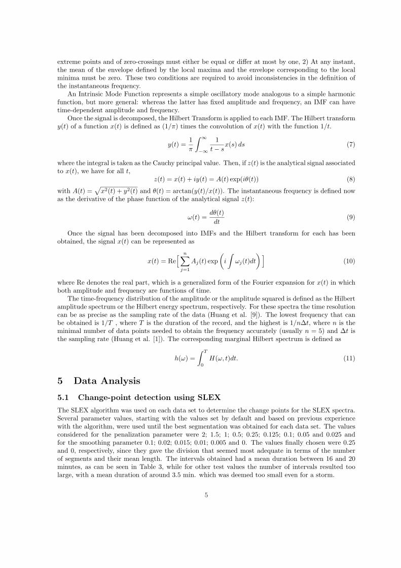
At the end of the original data set, where the completion with 0’s begins, SLEX produces spuriouschange-points that reflect the change from data to a constant, as can be seen in Figure 4, hence thelast change-point considered is the one previous to the end of the data set.

For the first data set Storm1999a 30 change-points were obtained; for the second Storm1999b, 24;for the third Storm1999c, 60, for the fourth Storm1999d and the fifth Storm1999e, 72 for each. Table3gives some basic statistics for the length of the intervals obtained for each data set.

Figure 5 shows boxplots for interval length for each data set.

6

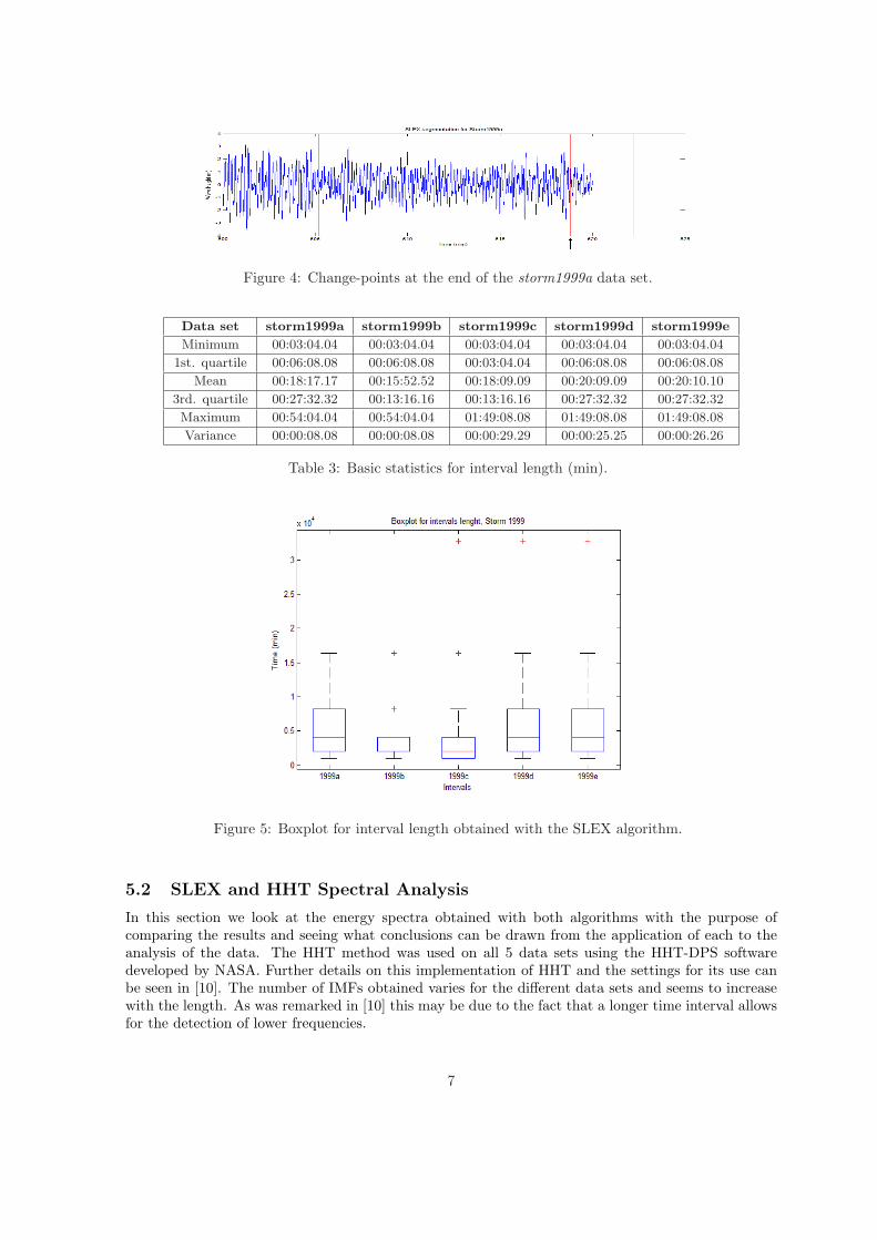
Figure 4: Change-points at the end of the storm1999a data set.

Data set storm1999a storm1999b storm1999c storm1999d storm1999e

Minimum 00:03:04.04 00:03:04.04 00:03:04.04 00:03:04.04 00:03:04.04

1st. quartile 00:06:08.08 00:06:08.08 00:03:04.04 00:06:08.08 00:06:08.08

Mean 00:18:17.17 00:15:52.52 00:18:09.09 00:20:09.09 00:20:10.10

3rd. quartile 00:27:32.32 00:13:16.16 00:13:16.16 00:27:32.32 00:27:32.32

Maximum 00:54:04.04 00:54:04.04 01:49:08.08 01:49:08.08 01:49:08.08

Variance 00:00:08.08 00:00:08.08 00:00:29.29 00:00:25.25 00:00:26.26

Table 3: Basic statistics for interval length (min).

Figure 5: Boxplot for interval length obtained with the SLEX algorithm.

5.2 SLEX and HHT Spectral Analysis

In this section we look at the energy spectra obtained with both algorithms with the purpose ofcomparing the results and seeing what conclusions can be drawn from the application of each to theanalysis of the data. The HHT method was used on all 5 data sets using the HHT-DPS softwaredeveloped by NASA. Further details on this implementation of HHT and the settings for its use canbe seen in [10]. The number of IMFs obtained varies for the different data sets and seems to increasewith the length. As was remarked in [10] this may be due to the fact that a longer time interval allowsfor the detection of lower frequencies.

7

Data set Duration Num. IMF’sStorm1999a 8h. 40m. 17Storm1999b 6h. 15Storm1999c 18h. 19Storm1999d 24h. 21Storm1999e 24h. 20

Table 4: Number of IMFs for each data set.

For each of the five data sets the marginal Hilbert spectrum was calculated. Further, for eachsegment obtained with the SLEX algorithm, both the SLEX spectrum and the classical Fourier spec-trum were calculated. The Fourier spectra were obtained using the WAFO software. Figure 7 showsthe SLEX spectrogram for the Storm1999a data set and figure 6 gives the boxplots for the energymaxima obtained with the HHT algorithm for each SLEX segment. The SLEX spectrogram has asimilar interpretation to the usual Fourier spectrogram.

Figure 6: Boxplots for maximal HHT energy in each segment for the five data sets.

We look now at the behaviour of the Hilbert spectrum around the change points detected usingthe SLEX algorithm. We looked both at the Hilbert spectrum and the marginal Hilbert spectrum ina neighbourhood of the change points, taking 300 data points (equivalent to 60 secs.) on each sideof the change-point, for a total time of 2 min. We comment, using the results for the first data setStorm1999a. For most change-points there are noticeable changes in the energy. For 20 of the 28change-points the changes are pronounced; in 8 of them the energy increases and in the remaining 12it decreases. Figures 8 and 9 shows examples of both situations. For the other 8 change-points thechange is not as pronounced, although changes in the total energy can be observed. An example ofthis is given in Figure 10

5.3 An analysis of results for ’Large’ Waves

In this section we analyze the energy spectra and their evolution for large waves, i.e. for waveshigher than 6.5 m. Table 5 gives the location of these events, their height and the total energy in aneighbourhood of the event comprising 150 data points, corresponding to 30 seconds, with the maximalpoint at the centre. The mean wave period is about 11 s.

8

Figure 7: SLEX Spectrogram for the Storm1999a data set.

Figure 8: Hilbert and marginal Hilbert spectra for a neighbourhood of change-point 6 for theStorm1999a data set

Figure 9: Hilbert and marginal Hilbert spectra for a neighbourhood of change-point 9 for theStorm1999a data set

Figures 11 to 15 give the Hilbert and marginal Hilbert spectra for some large waves. Figure 11(top) corresponds to the Hilbert spectrum for the seventh SLEX interval of Storm1999a, which showsthe energy evolution for the interval. One can see large amounts of energy near the endpoints ofthe interval located approximately at 82 and 95 min. and with energy reaching 0.6m2s/rad and0.75m2s/rad, respectively. These two events correspond to large waves 1 and 2 and are singled-out

9

Figure 10: Hilbert and marginal Hilbert spectra for a neighbourhood of change-point 4 for theStorm1999a data set

Data set Data point Time (min) Height (m) Energy (HHT)1999a Wave 1 24705 82.3 6.93 45.36

Wave 2 28562 95.2 6.61 33.581999c Wave 1 260365 867.9 6.62 43.75

Wave 2 273146 910.5 6.57 29.54Wave 3 279587 932.0 6.94 57.64Wave 4 316510 1055.0 7.66 44.28

1999d Wave 1 22885 76.3 6.91 17.73Wave 2 23765 79.2 6.88 33.54Wave 3 24653 82.2 7.27 24.44Wave 4 70298 234.3 6.69 36.37Wave 5 74329 247.8 7.26 33.15Wave 6 77015 256.7 8.59 49.71Wave 7 89891 299.6 6.89 33.43Wave 8 92022 306.7 6.99 39.11Wave 9 171602 572.0 6.72 29.76

1999e Wave 1 51695 172.3 6.69 38.86

Table 5: Large waves

in the bottom graphs. The total energy accumulated in a 30 second neighbourhood of large wave 1 is45.39 m2s/rad while for large wave 2 it is 33.58m2s/rad.

Figure 12 shows a colour-coded contour graph for the Hilbert spectra for large waves 1 and 2 ofStorm1999a at the top and the actual waves at the bottom with the same time scale. The figure forlarge wave 1 shows that there is a large amount of energy around this event. In contrast, the graphfor large wave 2 shows a large amount of energy after the wave, in the time interval between 5720 and5725 secs.

Figure 13 (top) shows the Hilbert spectrum for the second SLEX interval for Storm1999d and(bottom) the corresponding spectra for large waves 1 and 2 of that interval. The top graph givesthe evolution of the energy during the whole interval, which includes large waves 1 and 2 roughly at76 and 79 minutes, towards the right-hand end of the interval. The bottom graphs show the energyaround these events. The total energy accumulated in a 30 second neighbourhood of large wave 1 is17.7316m2s/rad while for large wave 2 it is 33.54m2s/rad.

Figure 14 shows a contour graph for the Hilbert spectrum (top) for interval 2 of the SLEX seg-mentation of Storm1999d, covering a total of 27.3 min. On the bottom there is a graph of wave heightfor the same interval using the same time scale. There are two large waves in this interval, the first

10

Figure 11: (top) Hilbert spectrum for interval 7 of Storm1999a. (bot.) Hilbert spectra for large waves1 and 2.

Figure 12: Contour graph for the Hilbert spectra for large waves 1 and 2 of Storm1999a. The actualwaves are shown below.

one around 76.3 min. and the second around 79.2 min. For the first wave frequencies are distributedbetween 0.05 and 0.2 Hz. in a 30 second neighbourhood of the maxima. For the second the energyis more concentrated around 0.05 Hz. and for the 30 second neighbourhood of this wave the energyvaries between 0.05 and 0.3 Hz. Both waves are the result of the superposition of several Intrinsic ModeFunctions, none of which has a large amount of energy associated (see Figure 15). This phenomenonwas also observed and commented in [9].

6 Conclusions

We have used the SLEX and HHT algorithms for the segmentation and spectral analysis of wave datarecorded during a storm that took place in the North Sea in 1999. The data was divided into 5 setslasting between 6 and 24 hours, as shown in Table 1. Each data set was segmented into stationaryintervals using SLEX and the corresponding SLEX spectra were calculated. Using the software HHT-

11

Figure 13: (top) Hilbert spectrum for interval 2 of Storm1999d. (bot.) Hilbert spectra for large waves1 and 2.

Figure 14: Contour graph for the Hilbert spectra for interval 2 of Storm1999d. Wave heights for thewhole interval are shown below.

DPS each data set was decomposed into Intrinsic Mode Functions and the corresponding Hilbertspectra were obtained. For each interval obtained in the SLEX segmentation the marginal Hilbertspectra were calculated.

The SLEX algorithm is very useful for finding change points of a large set of data, as in this work,looking at changes in the spectral distribution of energy. SLEX divides the data set into segments thatare approximately stationary. One disadvantage of this method is that the length of the data set mustbe a power of two (L = 2N ). However, this can solved either by completing the data set with zeros upto the next power of two or truncating the data set at the largest power of two less than the lengthof the data set. Both methods were used in this work and common data subset the change pointscoincided, so that the first method, which covers the whole data set, was preferred. It is importantto observe that the completion with zeros may produce false change points near the end of the dataset. Another limitation of SLEX is that, since it needs to calculate the spectra of subsets of the dataset in order to compare the energy distribution in each one, the subsets must have enough data points

12

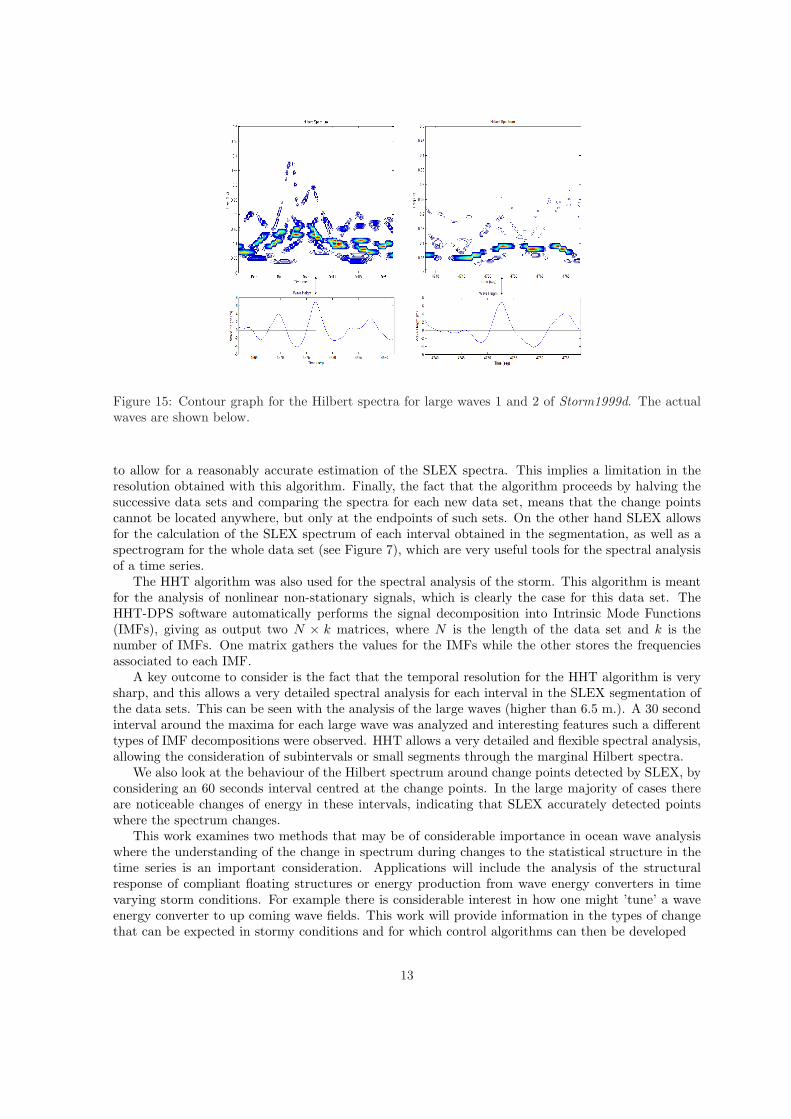
Figure 15: Contour graph for the Hilbert spectra for large waves 1 and 2 of Storm1999d. The actualwaves are shown below.

to allow for a reasonably accurate estimation of the SLEX spectra. This implies a limitation in theresolution obtained with this algorithm. Finally, the fact that the algorithm proceeds by halving thesuccessive data sets and comparing the spectra for each new data set, means that the change pointscannot be located anywhere, but only at the endpoints of such sets. On the other hand SLEX allowsfor the calculation of the SLEX spectrum of each interval obtained in the segmentation, as well as aspectrogram for the whole data set (see Figure 7), which are very useful tools for the spectral analysisof a time series.

The HHT algorithm was also used for the spectral analysis of the storm. This algorithm is meantfor the analysis of nonlinear non-stationary signals, which is clearly the case for this data set. TheHHT-DPS software automatically performs the signal decomposition into Intrinsic Mode Functions(IMFs), giving as output two N × k matrices, where N is the length of the data set and k is thenumber of IMFs. One matrix gathers the values for the IMFs while the other stores the frequenciesassociated to each IMF.

A key outcome to consider is the fact that the temporal resolution for the HHT algorithm is verysharp, and this allows a very detailed spectral analysis for each interval in the SLEX segmentation ofthe data sets. This can be seen with the analysis of the large waves (higher than 6.5 m.). A 30 secondinterval around the maxima for each large wave was analyzed and interesting features such a differenttypes of IMF decompositions were observed. HHT allows a very detailed and flexible spectral analysis,allowing the consideration of subintervals or small segments through the marginal Hilbert spectra.

We also look at the behaviour of the Hilbert spectrum around change points detected by SLEX, byconsidering an 60 seconds interval centred at the change points. In the large majority of cases thereare noticeable changes of energy in these intervals, indicating that SLEX accurately detected pointswhere the spectrum changes.

This work examines two methods that may be of considerable importance in ocean wave analysiswhere the understanding of the change in spectrum during changes to the statistical structure in thetime series is an important consideration. Applications will include the analysis of the structuralresponse of compliant floating structures or energy production from wave energy converters in timevarying storm conditions. For example there is considerable interest in how one might ’tune’ a waveenergy converter to up coming wave fields. This work will provide information in the types of changethat can be expected in stormy conditions and for which control algorithms can then be developed

13

7 Acknowledgements

The authors would like to thank Total E&P UK for the wave data from the Alwyn North platform.The Hilbert-Huang transform Data Processing System whose copyright is with the United States Gov-ernment as represented by the Administrator of the National Aeronautics and Space Administration,was used with permission. The software WAFO [1] developed by the Wafo group at Lund Univer-sity of Technology, Sweden was used for the calculation of all Fourier spectra and associated spectralcharacteristics. This software is available at http://www.maths.lth.se/matstat/wafo. This work waspartially supported by CONACYT, Mexico, Proyecto Analisis Estadıstico de Olas Marinas. This workwas partially done while the first author visited CIMAT. The support of CIMAT and the UniversidadCentral de Venezuela are gratefully acknowledge. George Smith would like to gratefully acknowledgethe support offered by Scottish and Southern Energy PLC.

References

[1] P.A. Brodtkorb, P. Johannesson, G. Lindgren, I. Rychlik, E. Ryden, and E. Sjo. Wafo - a matlabtoolbox for analysis of random waves and loads. In Proc. 10th Int. Offshore and Polar Eng. Conf.,volume III, pages 343–350, Seattle, USA, 2000. ISOPE, ISOPE.

[2] R. Coifman and M. Wickerhauser. Entropy based algorithms for best basis selection. IEEE Trans.on Information Theory, 32:712–718, 1992.

[3] N.E. Huang. Hilbert-Huang Transform and Its Applications., chapter Introduction to Hilbert-Huang Transform and its related mathematical problems, pages 1–26. World Scientific, 2005.

[4] N.E. Huang. The Hilbert-Huang transform in Engineering, chapter Introduction to Hilbert-HuangTransform and some recent developments, pages 1–23. CRC Press, 2005.

[5] N.E. Huang, Z. Shen, and S.R. Long. A new view of nonlinear water waves: the hilbert spectrum.Ann Rev Fluid Mech, 31:417–57, 1999.

[6] N.E. Huang, M.L. Wu, S.R. Long, S.P. Shen, W.Q. Per, P. Gloersen, and K.L. Fan. A confidencelimit for the empirical mode decomposition and hilbert spectral analysis. Proceedings of the RoyalSociety of London, 459:2317–45, 2003.

[7] N.E.Huang, Z. Shen, S.R. Long, M.C. Wu, H.S. Shin, Q. Zheng, Y. Yuen, C.C. Tung, and H.H.Liu. The empirical mode decomposition and hilbert spectrum for nonlinear and non-stationarytime series analysis. Proceedings of the Royal Society of London, 454:903–995, 1998.

[8] H. Ombao, J. Raz, R. Von Sachs, and W. Guo. The slex model of a non-stationary randomprocess. Ann. Inst. Statist. Math., 52(1):1–18, 2002.

[9] J. Ortega and George H. Smith. Spectral analysis of storm waves using the hilbert-huang trans-form. In Proceedings of the Seventeenth International Offshore and Polar Engineering Conference.,pages 1830–1835. ISOPE, 2007.

[10] J. Ortega and George H. Smith. Hilbert-huang transform analysis of storm waves. Applied OceanRes., 31:212–219, 2009.

[11] J. Wolfram, G. Feld, and J. Allen. A new approach to estimating environmental loading usingjoint probabilities. In 7th Int. Conf. on Behaviour of Offshore Structures, pages 701–713, Boston,1994. Pergamon.

14