Spectral Algorithms II - Computer...
42
Applications Spectral Algorithms II Applications Slides based on “Spectral Mesh Processing” Siggraph 2010 course
Transcript of Spectral Algorithms II - Computer...

Applications
Spectral Algorithms IIApplications
Slides based on “Spectral Mesh Processing” Siggraph 2010 course
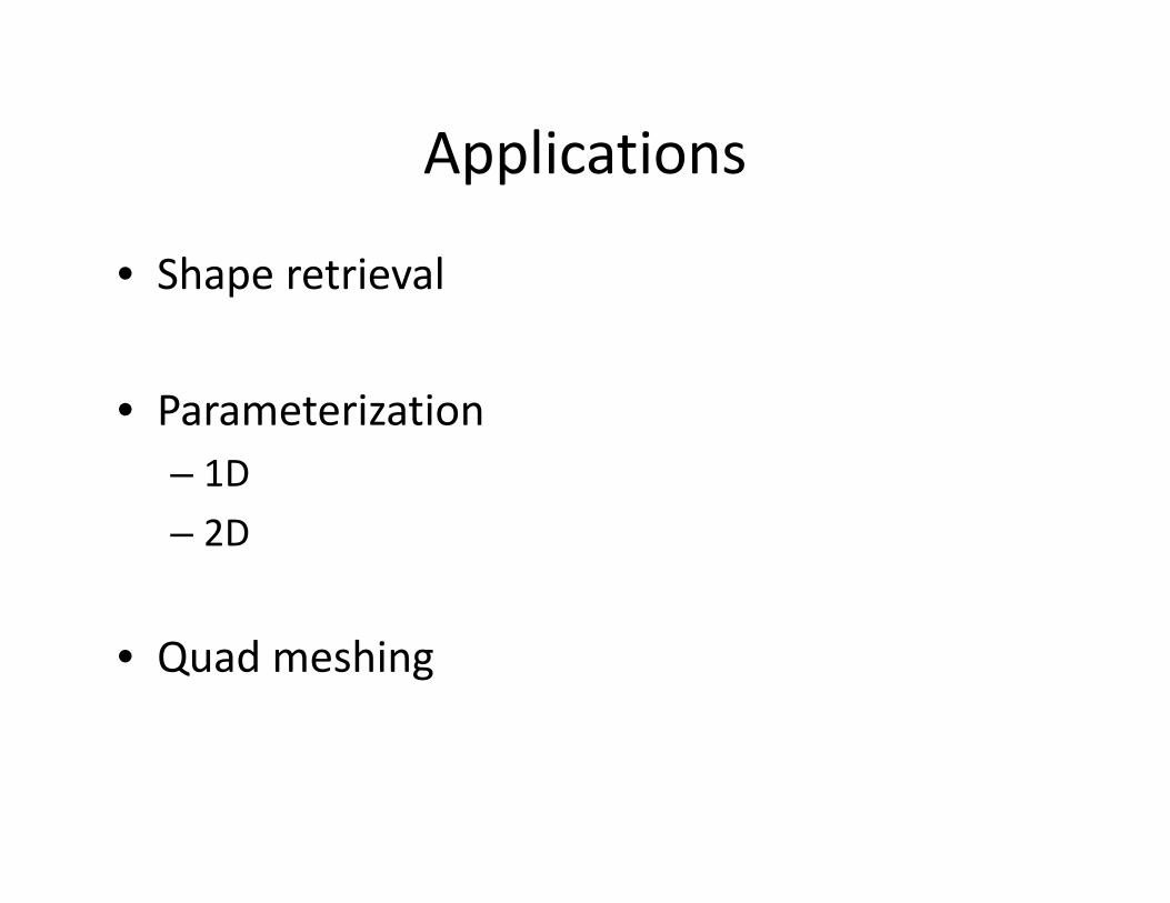
ApplicationsApplications
• Shape retrievalShape retrieval
i i• Parameterization– 1D
– 2D
• Quad meshing

Shape RetrievalShape Retrieval
3D R it Q M h3D Repository Query Matches

Descriptor based shape retrievalDescriptor based shape retrieval
3D R it d i t Q d i t Cl t t h3D Repository descriptors Query descriptor Closest matches

Pose Invariant Shape Descriptorp p
“Similar” descriptors for shape in different poses
Cat Same cat Still the same cat
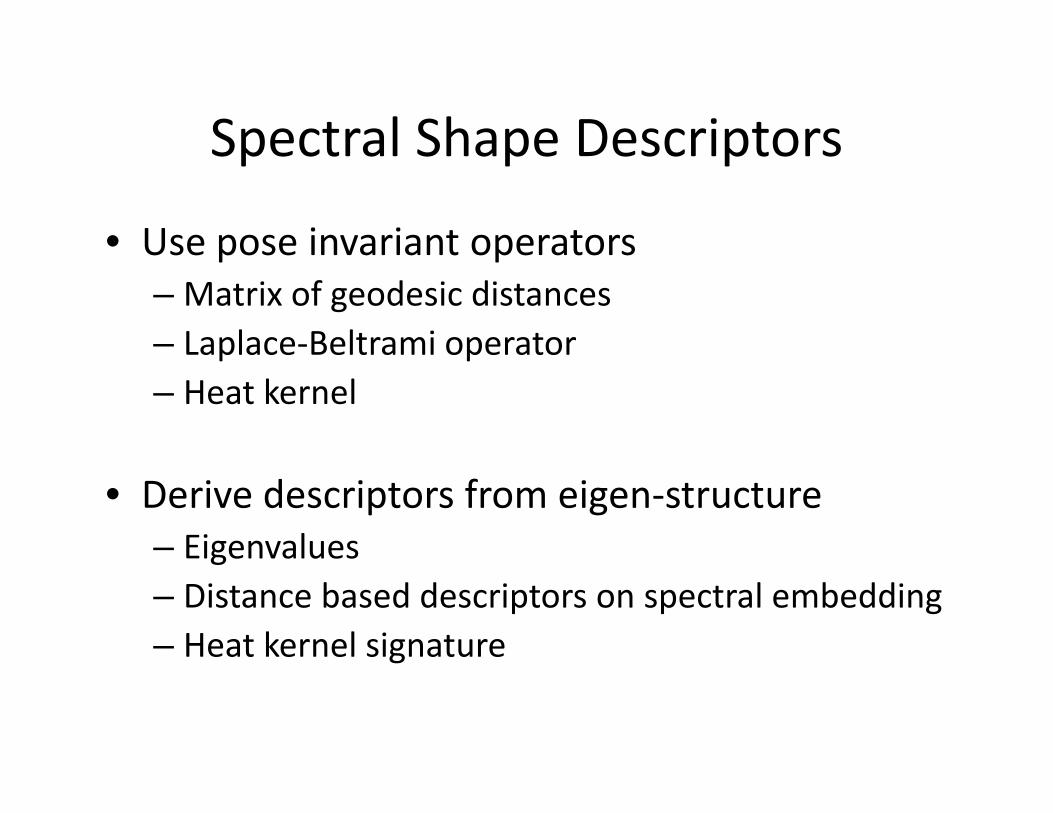
Spectral Shape DescriptorsSpectral Shape Descriptors
• Use pose invariant operatorsUse pose invariant operators– Matrix of geodesic distances– Laplace‐Beltrami operatorp p– Heat kernel
• Derive descriptors from eigen‐structure– Eigenvaluesg– Distance based descriptors on spectral embedding– Heat kernel signatureg
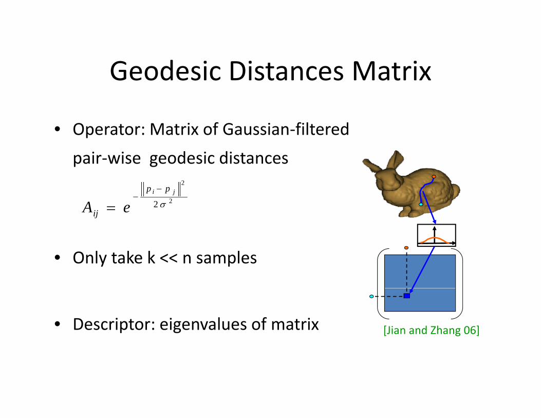
Geodesic Distances MatrixGeodesic Distances Matrix
• Operator: Matrix of Gaussian‐filtered• Operator: Matrix of Gaussian‐filtered
pair‐wise geodesic distances 2
2
2
2σji pp
ij eA−
−=
• Only take k << n samples
• Descriptor: eigenvalues of matrix [Jian and Zhang 06]
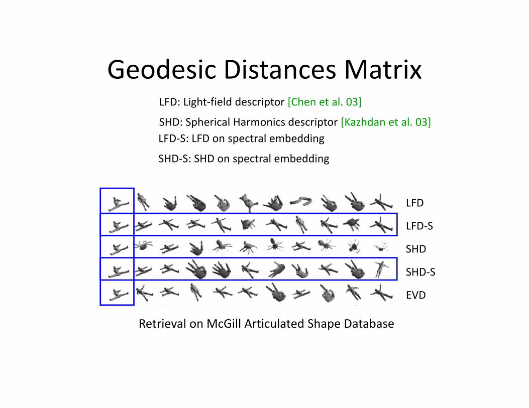
Geodesic Distances MatrixGeodesic Distances MatrixLFD: Light‐field descriptor [Chen et al. 03]
SHD: Spherical Harmonics descriptor [Kazhdan et al. 03]p p [ ]LFD‐S: LFD on spectral embedding
SHD‐S: SHD on spectral embedding
LFD
LFD‐S
SHD
SHD‐S
Retrieval on McGill Articulated Shape Database
EVD
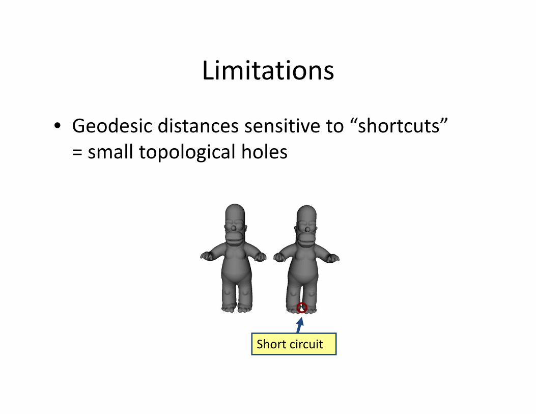
LimitationsLimitations
• Geodesic distances sensitive to “shortcuts”Geodesic distances sensitive to shortcuts= small topological holes
Short circuit

Global Point Signatures [Rustamov 07]Global Point Signatures [Rustamov 07]
Given a point p on the surface, define
– φi(p) value of the eigenfunction φi at the point p
– λi’s are the Laplace‐Beltrami eigenvalues
– Euclidean distance in GPS space =
commute time distance on the surface

GPS-based shape retrievalGPS based shape retrieval
• Use histogram of distances in• Use histogram of distances in
the GPS embeddings
– Invariance properties reflected
in GPS embeddings
– Less sensitive to topology– Less sensitive to topology
changes by using only low‐
frequency eigenfunctions Short circuitfrequency eigenfunctions
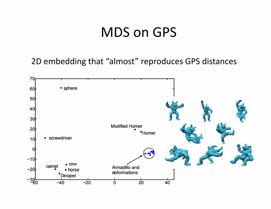
MDS on GPS
2D embedding that “almost” reproduces GPS distancesg p

Use for shape matching?Use for shape matching?
• Nope. Embedding sensitive to eigenvectorNope. Embedding sensitive to eigenvector “switching”
• Eigenvectors are not uniqueOnly defined up to sign– Only defined up to sign
– If repeating eigenvalues – any vector in subspace is eigenvectoris eigenvector

Heat Equation on a ManifoldHeat Equation on a Manifold
Heat kernel
: amount of heat transferred from to in time .
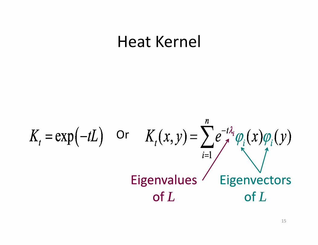
Heat KernelHeat Kernel
OrOr
Eigenvalues Eigenvalues ofof LL
EigenvectorsEigenvectorsofof LL
15
of of LL of of LL
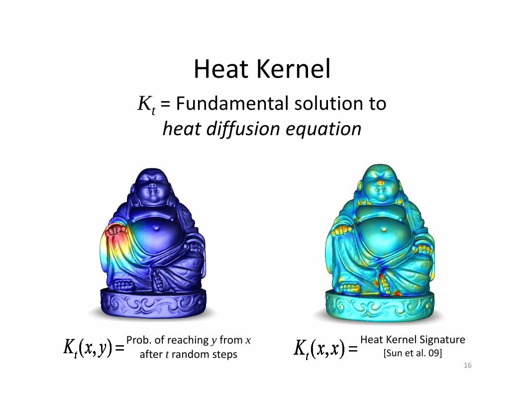
Heat KernelKt = Fundamental solution to
heat diffusion equation
Heat Kernel
heat diffusion equation
Prob. of reaching y from xafter t random steps
Heat Kernel Signature[Sun et al. 09]
16

Heat Kernel SignatureHeat Kernel Signature
HKS(p) = : amount of heat left at p at time t.p pSignature of a point is a function of one variable.
Invariant to isometric deformations. Moreover complete:
Any continuous map between shapes that preserves HKS must y p p ppreserve all distances.
A Concise and Provably Informative …,Sun et al., SGP 2009
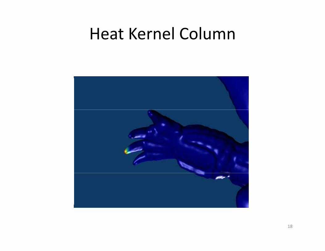
Heat Kernel Column
18

Heat Kernel Signature
19

Heat Kernel Applied
• Diffusion wavelets
Heat Kernel Applied
[Coifman and Maggioni ‘06]
• Segmentation [deGoes et al ‘08][deGoes et al. 08]
• Heat kernel signature [Sun et al. ‘09][ ]
• Heat kernel matching [Ovsjanikov et al. ’10]
20

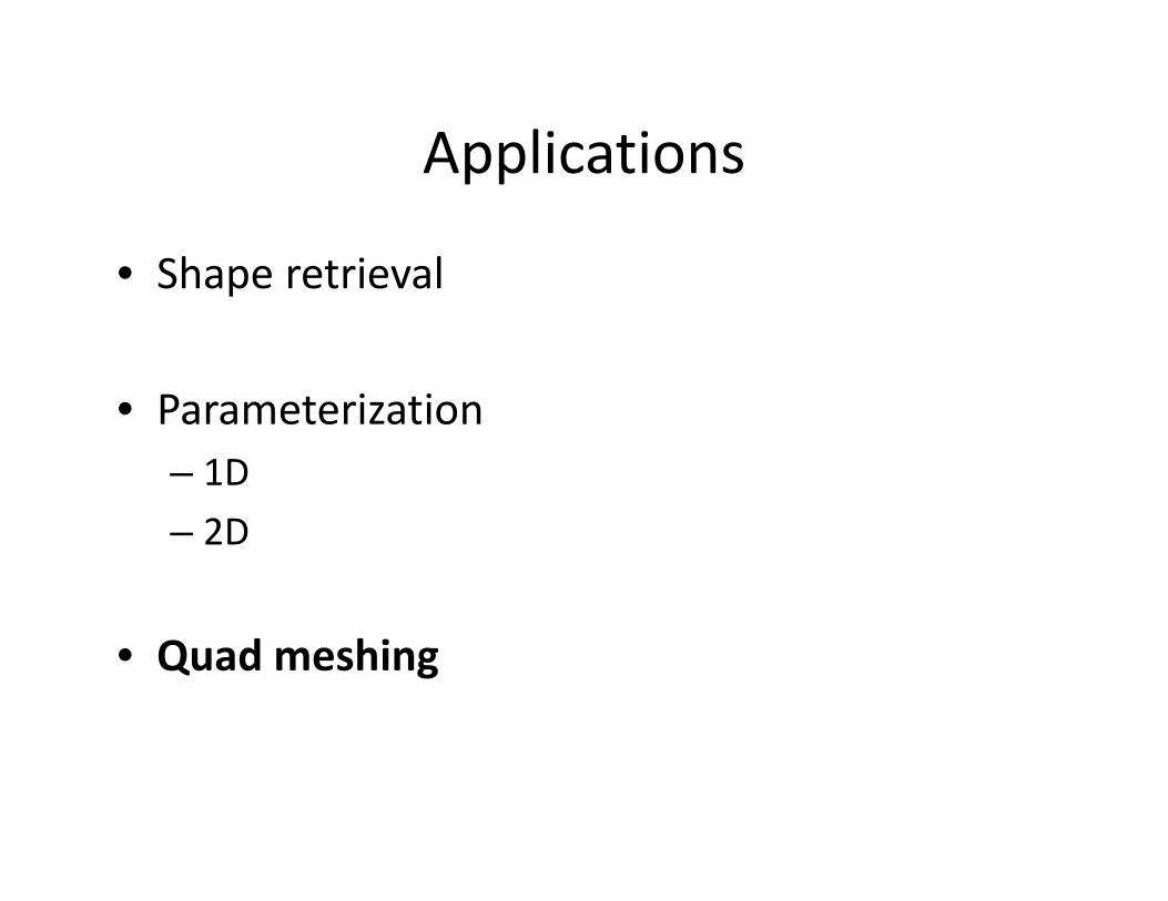
ApplicationsApplications
• Shape retrievalShape retrieval
i i• Parameterization– 1D
– 2D
• Quad meshing

1D surface parameterizationGraph Laplacian
ai,j = wi,j > 0 if (i,j) is an edge
a = Σ aai,i = ‐Σ ai,j
(1,1 … 1) is an eigenvector assoc. with 0(1,1 … 1) is an eigenvector assoc. with 0
The second eigenvector is interresting[Fiedler 73, 75]

1D surface parameterizationFiedler vector
FEM i R d i hFEM matrix,Non‐zero entries
Reorder withFiedler vector

1D surface parameterizationFiedler vector
Streaming meshes [Isenburg & Lindstrom][Isenburg & Lindstrom]

1D surface parameterizationFiedler vector
Streaming meshes [Isenburg & Lindstrom][Isenburg & Lindstrom]

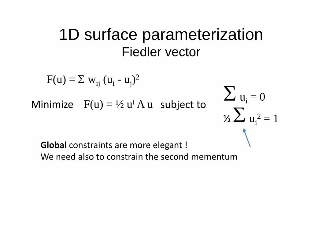
1D surface parameterizationFiedler vector
F( ) Σ ( )2
F(u) = ½ ut A uMinimize
F(u) = Σ wij (ui - uj)2
( )

1D surface parameterizationFiedler vector
F( ) Σ ( )2
F(u) = ½ ut A uMinimize
F(u) = Σ wij (ui - uj)2
( )
How to avoid trivial solution ?Constrained vertices ?

1D surface parameterizationFiedler vector
F( ) Σ ( )2
Σ ui = 0F(u) = ½ ut A uMinimize subject to
F(u) = Σ wij (ui - uj)2
( ) j
Global constraints are more elegant !
1D surface parameterizationFiedler vector
F( ) Σ ( )2
Σ ui = 0
ΣF(u) = ½ ut A uMinimize subject to
F(u) = Σ wij (ui - uj)2
½ Σ ui2 = 1
( ) j
Global constraints are more elegant !We need also to constrain the second mementum

1D surface parameterizationFiedler vector
F( ) Σ ( )2
Σ ui = 0
ΣF(u) = ½ ut A uMinimize subject to
F(u) = Σ wij (ui - uj)2
½ Σ ui2 = 1
( ) j
L(u) = ½ ut A u - λ1 ut 1 - λ2 ½ (utu - 1)( ) 1 2 ( )
∇u L = A u - λ1 1 - λ2 u u = eigenvector of A∇λ1L = ut 1∇λ2L = ½(ut u – 1)
λ1 = 0λ2 = eigenvalue

1D surface parameterizationFiedler vector
Rem: Fiedler vector is also a minimizer of the Rayleigh quotient
R(A,x) =
xt x
xt A x
The other eigenvectors xi are the solutions of :
minimize R(A,xi) subject to xit xj = 0 for j < i ( , i) j i j j

Surface parameterization
Minimize
22∂∂ uu∂∂ yy--
∂∂ vv∂∂ xxΣΣ Discrete conformal mapping:
Minimize∂∂ uu∂∂ xx
∂∂ vv∂∂ yy
yy--ΣΣ
TT [L, Petitjean, Ray, Maillot 2002][Desbrun, Alliez 2002]

Surface parameterization
Discrete conformal mapping:Minimize
22∂∂ uu∂∂ yy--
∂∂ vv∂∂ xxΣΣ
[L, Petitjean, Ray, Maillot 2002][Desbrun, Alliez 2002]
Minimize∂∂ uu∂∂ xx
∂∂ vv∂∂ yy
yy--ΣΣ
TT
Usespinned points.

Sensitive to Pinned VerticesSensitive to Pinned Vertices

Surface parameterization
[Muellen, Tong, Alliez, Desbrun 2008]
Use Fiedler vector,i.e. the minimizer of R(A,x) = xt A x / xt x that is orthogonal to the trivial constant solutionthat is orthogonal to the trivial constant solution
Implementation: (1) assemble the matrix of the discrete conformal parameterization( ) d h h f l(2) compute its eigenvector associated with the first non‐zero eigenvalue
See http://alice.loria.fr/WIKI/ Graphite tutorials – Manifold Harmonics
ApplicationsApplications
• Shape retrievalShape retrieval
i i• Parameterization– 1D
– 2D
• Quad meshing

Chladni PatternsChladni Patterns
Nodal sets of eigenfunctions of LaplacianNodal sets of eigenfunctions of Laplacian

Chladni PatternsChladni Patterns

Quad RemeshinggNodal sets are sets of curves intersecting at constant anglesNodal sets are sets of curves intersecting at constant angles
The NThe N th eigenfunction has at most N eigendomainsth eigenfunction has at most N eigendomainsThe NThe N--th eigenfunction has at most N eigendomainsth eigenfunction has at most N eigendomains

Surface quadrangulationg
One eigenfunction Morse complex Filtered morse complexOne eigenfunction Morse complex Filtered morse complex
[Dong and Garland 2006]

Surface quadrangulationg
Reparameterization of the quads

Surface quadrangulationg
Improvement in [Huang, Zhang, Ma, Liu, Kobbelt and Bao 2008], takes a guidance vector field into account.