Spectral Aanalysis and Quantitation in MALDI-MS …Tina Memo No. 2015-016 PhD Thesis. Spectral...
109
Tina Memo No. 2015-016 PhD Thesis. Spectral Aanalysis and Quantitation in MALDI-MS Imaging. Somrudeee Deepaisarn. Last updated 8 /10 / 2018 Imaging Science and Biomedical Engineering Division, Medical School, University of Manchester, Stopford Building, Oxford Road, Manchester, M13 9PT.
Transcript of Spectral Aanalysis and Quantitation in MALDI-MS …Tina Memo No. 2015-016 PhD Thesis. Spectral...

Tina Memo No. 2015-016
PhD Thesis.
Spectral Aanalysis and Quantitation in MALDI-MSImaging.
Somrudeee Deepaisarn.
Last updated8 /10 / 2018
Imaging Science and Biomedical Engineering Division,Medical School, University of Manchester,
Stopford Building, Oxford Road,Manchester, M13 9PT.

SPECTRAL ANALYSIS AND QUANTITATION
IN MALDI-MS IMAGING
FIRST YEAR CONTINUATION REPORT
SOMRUDEE DEEPAISARN
INSTITUTE OF POPULATION HEALTH
SCHOOL OF MEDICINE, THE UNIVERSITY OF MANCHESTER
2015
SUPERVISORS
DR. ADAM MCMAHON
DR. NEIL THACKER

2
Preface I have been studying at the University of Manchester since 2010. In 2013, I
completed a BSc in Physics from the School of Physics and Astronomy. Then, I attended an
MSc Medical Imaging programme in the School of Medicine (2013-2014). From the MSc
course, I met Dr. Adam McMahon and Dr. Neil Thacker who became my supervisors of my
PhD project named “Spectral analysis and quantitation in MALDI-MS imaging”. The PhD
course is imaging plan, in Institute of Population Health (IPH), School of Medicine.
This PhD programme provides me an opportunity to work in real research
environment in a laboratory based in the Wolfson Molecular Imaging Centre (WMIC)
building, surrounded with people from various imaging areas. During the first year of my
PhD course, I learnt a lot of new analytical techniques. Beginning with no mass spectrometry
experience, I developed skills using MALDI-MS, including practice how to prepare good
samples, understand the instrumentation, and generate MS data on which I have done
some quantitative tests. Moreover, I have practiced tandem MS technique which will take
part in next year experiments. Also, MS images were successfully generated from the
acquired MSI data. I used some higher performance instruments at KRATOS analytical
laboratory, Manchester a couple of times this year and will be used more in the following
years.
This first year continuation report will follow the Master thesis style. It is an
appropriate way of presenting my project at this stage as it will show relevant background
covering from basic knowledge to reviews of literature in the project area, following by clear
description of methodology, results and discussion, and summary of future work.
List of conferences and courses attended
Speed PhD course, University of Manchester
Meetings and Showcases by IPH and School of Medicine, University of Manchester
Royal Society of Chemistry Analytical Awards Symposium, University of Manchester
British Mass Spectrometry Society annual meeting 2015 and a course on
introduction to mass spectrometry, University of Birmingham
NanoSIMS International Workshop 2015, University of Manchester

3
Abstract Mass spectrometry (MS) is an analytical technique that can determine the mass-to-
charge ratio (m/z) of analytes. Matrix-assisted laser desorption/ionisation (MALDI) is a soft
ionisation technique for MS, beneficial in ionising large (biological) molecules which have
low volatility. It is usually combined with a time-of-flight mass analyser measuring of ion
current signal versus m/z which is represented as a mass spectrum. To perform MS imaging,
mass spectral data are acquired across a sample area. Then, a 2-dimensional image can be
constructed out of mass spectral information at an array of known spatial locations. Analyte
structural determination is also possible via tandem MS yielding a spectrum of fragment
ions from the precursor ion of specific m/z, aiding identification of analyte molecules.
This project is a study of spectral analysis and quantitation in MALDI-MS imaging. It
aims to develop quantitative methods of analysis for lipid molecules in tissue using MALDI-
MS imaging to identify markers for some diseases. The primary target tissue to be studied is
the brain, which is known to be lipid-rich. Lipids are present in all tissues, not only to form
their structures but also play important part in metabolism and signalling activities.
Investigating the presence of a particular lipid quantitatively at specific regions of body’s
tissue can potentially distinguish normal and abnormal characteristics. The initial
experiments have used lipid extracts from cow’s and goat’s milk samples as readily available
examples of complex lipid mixtures. An AXIMA Performance MALDI-TOF2-MS instrument
(Kratos, Shimadzu group) was used. Mass spectra were found to be significantly influenced
by preparation protocols and instrumental settings. Laser power is an important factor,
which varies laser fluence at the sample-matrix crystal causing the initial ionization event
that generates ion signals. The laser power was adjusted to achieve appropriate signal-to-
noise ratios and kept constant throughout an experimental session. The current
quantification approach used the ratios of integrated area under specific m/z peaks to
estimate the relative concentration of 2 different analytes in a sample. Using analysis of
variance, it was observed that repeatability of peak area ratios (760.5 vs 734.5 m/z) was
improved when the sample and 2,5-dihydroxybenzoic acid (DHB) matrix solutions were
mixed in solution before deposition. A TLC spraying technique was used to apply sample-
matrix mixes onto both metal and indium tin oxide (ITO) coated glass surface, for varied
concentrations of cow’s and goat’s milk mixtures. These showed a consistent linear
correlation in area ratio of particular peaks (760.5 vs 706.5 m/z). Three approaches for
matrix application on typical glass slides were compared as coating matrix on top of tissue
on ITO glass slide would be required in preparing MALDI-MS imaging samples. The TLC
sprayer apparatus was adjusted to achieve similar deposition conditions as used by the
SunCollect (SunChrom) matrix applicator. An alternative matrix application system using an
ultrasonic nebuliser was also assessed but found to be a highly matrix-consuming;
therefore, prohibitively expensive method. Good examples of MS images of rat brain tissue
section were generated when 10 mg/ml DHB matrix was deposited using the SunCollect and
MS data were acquired using the 7090 model MALDI-TOF2-MS (Kratos). The images show
clear variation in particular m/z peaks at different brain regions.

4
Contents Preface ....................................................................................................................................... 2
Abstract ...................................................................................................................................... 3
1. Introduction ......................................................................................................................... 15
2. Background .......................................................................................................................... 17
2.1 Mass Spectrometry ........................................................................................................ 17
2.1.1 General Background ................................................................................................ 17
2.1.2 Types of Mass Analysers .......................................................................................... 19
2.1.3 Ionisation Techniques .............................................................................................. 21
2.2 MALDI-TOF Mass Spectrometry ..................................................................................... 24
2.2.1 Invention .................................................................................................................. 24
2.2.2 The MALDI Ionisation .............................................................................................. 26
2.2.3 Ion Acceleration ....................................................................................................... 29
2.2.4 The Time-of-flight Mass Analyser ............................................................................ 30
2.2.5 Detector ................................................................................................................... 33
2.2.6 Mass Resolution ...................................................................................................... 34
2.2.7 MALDI Matrices ....................................................................................................... 35
2.2.8 Sample Preparation (Sample-matrix Depositions) .................................................. 36
2.2.9 Tandem Mass Spectrometry ................................................................................... 37
2.2.10 MALDI-MS Imaging ................................................................................................ 38
2.3 MALDI-MS for Lipid Applications ................................................................................... 39
2.3.1 Lipid Extraction Techniques ..................................................................................... 40
2.3.2 Spectral Analysis (in Lipid Classification) ................................................................. 41
2.3.3 Limitations and Challenges ...................................................................................... 44
2.3.4 Lipids in the Brain .................................................................................................... 45
2.3.5 Mass Spectrometry Imaging of Lipids ..................................................................... 46
2.4 Overview of Quantitative Spectral Analysis ................................................................... 49
2.4.1 Supporting Software for Mass Spectrometry .......................................................... 49
2.4.2 Quantitative MALDI-MS Analysis ............................................................................ 50
3. Materials and Methods ........................................................................................................ 59
3.1 Materials......................................................................................................................... 59
3.1.1 Chemicals ................................................................................................................. 59

5
3.1.2 Equipment ............................................................................................................... 59
3.1.3 Other Materials Descriptions .................................................................................. 60
3.2 Sample Preparations ...................................................................................................... 60
3.2.1 Preparation of Milk Samples ................................................................................... 60
3.2.2 Preparation of Matrix Solution ................................................................................ 61
3.2.3 Sample-Matrix Deposition Method for MS Analysis of Milk Samples .................... 61
3.2.4 Preparation of Rat Brain Tissue Samples ................................................................. 62
3.2.5 Matrix Deposition Method for Imaging Rat Brain Tissue Samples ......................... 62
3.2.6 Calibration Standard ................................................................................................ 63
3.3 MALDI-MS Apparatus Settings and Acquisition Parameters ......................................... 63
3.4 Experiments .................................................................................................................... 64
3.4.1 Initial Tests of Instrumental and Technical Performance ....................................... 64
3.4.2 Mass Spectra from Milk Samples ............................................................................ 64
3.4.3 Mass Spectrometry Imaging .................................................................................... 66
3.5 Pre-processing Analysis of Mass Spectra ....................................................................... 66
4. Results and Disscussion ....................................................................................................... 69
4.1 Initial Tests of Instrumental and Technical Performance .............................................. 69
4.1.1 Thickness of Sample-matrix Materials .................................................................... 69
4.1.2 Laser Power ............................................................................................................. 70
4.1.3 Calibration ............................................................................................................... 74
4.1.4 Discussion ................................................................................................................ 76
4.2 Mass Spectra from Milk Samples ................................................................................... 78
4.2.1 Repeatability Tests of MS Spectra from Milk Samples ............................................ 78
4.2.2 Measure of Milks’ Concentrations .......................................................................... 80
4.2.3 Characterisation of Milk Spectra (MS/MS) .............................................................. 81
4.2.4 Discussion ................................................................................................................ 84
4.3 Mass Spectrometry Imaging........................................................................................... 85
4.3.1 Comparison of Matrix Coating Techniques ............................................................. 85
4.3.2 Mass Spectrometry Imaging of Rat Brain Tissues ................................................... 87
4.3.3 Discussion ................................................................................................................ 89
5. Conclusions .......................................................................................................................... 90
6. Summary of Future Work .................................................................................................... 91

6
References ............................................................................................................................... 94
Appendix: MATLAB Codes...................................................................................................... 102

7
List of Tables
Table 2. 1 Main features for different types of optimised mass analysers ............................ 19
Table 2. 2 Laser sources for MALDI-MS .................................................................................. 27
Table 2. 3 Classification methods for mass spectrometry image analysis ............................. 55
Table 3. 1 List of chemicals used in experiments.................................................................... 59
Table 4. 1 Summary of ANOVA for peak area ratios (760.5 vs 734.5 m/z) resulted from
different sample-matrix deposition methods ......................................................................... 79
Table 4. 2 Estimated DHB matrix quantity deposited on glass slide using different
application methods ................................................................................................................ 86
Table 6. 1 A second year plan of the research project ........................................................... 92
8
List of Figures
Figure 2. 1 Desorption/ionisation process (diagram from: Lewis et al. (2006)) ..................... 28
Figure 2. 2 A simple diagram for orthogonal acceleration time-of-flight mass spectrometer
.................................................................................................................................................. 31
Figure 2. 3 Tandem TOF/TOF mass spectrometer combining linear and curved field
reflectron TOF mass analysers (Picture from : Cornish and Cotter (1993) ) .......................... 38
Figure 2. 4 (a) A ω-3 fatty acid where n in the Figure indicate a number of repeated CH2
(with single bond C-C) (Adapted from : Berg et al. (2002)) (b) cis and trans structures ........ 39
Figure 2. 5 MALDI-MS spectra of milk sample with an expanded view appearing brominated
C(36:1) and C(38:1) (Picture from : Picariello et al. (2007)) .................................................... 42
Figure 2. 6 MALDI-MS spectra for triacylglecerol (12:0/14:0/14:0) using positive ion mode
(Picture from : Al-saad et al. (2003)) ....................................................................................... 43
Figure 2. 7 MALDI-MS spectra of phospholipids samples (a) 1-palmitoyl-2-oleoyl-sn-
phosphatidylglycerol, (b) 1-palmitoyl-2-oleoyl-sn-phosphatidylethanoamine, (c) 1-palmitoyl-
2-oleoyl-sn-phosphatidylcholine, and (d) mixture of equal fractions of this 3 lipids with DHB
matrix, acquired using positive ion mode (picture from : Fuchs et al. (2009)) ....................... 44
Figure 2. 8 Transverse section of Human vs rat brains (pictures from: Davis (1913) and
Bennett et al. (1964), respectively) ......................................................................................... 46
Figure 2. 9 Mass spectrometry imaging steps (Diagram from: Murphy and Merrill (2011)) 47
Figure 2. 10 A mass spectrometry image indicating potassiated PC(16:0a/16:0) distributions
for sagittal slice of mouse brain with labels of brain parts ..................................................... 48
Figure 2. 11 Main components of a mass spectrum (Picture from : Müller et al. (2001)) ..... 51
Figure 2. 12 Calibration curve for insulin where the internal standard is des-pentapeptide
insulin (Picture from: Wilkinson et al (1997)) .......................................................................... 53
9
Figure 2. 13 (a) Decision tree characteristics where f1 and f2 are feature values of 2
different features at each node used as classification threshold (b) Plots of data with
decision boundaries being the feature values in the corresponding trees ............................. 57
Figure 2. 14 Principal component plot showing clusters of human serum examination using
mass spectrometry where red and green spots represent data from healthy and gastric
cancer training sets, respectively, and the blue spots represent data from testing sets (all
from gastric cancer patients) (Adapted from : Shao et al. (2012)) .......................................... 58
Figure 3. 1 Diagram for ultrasonic nebulizing apparatus for matrix application where the
ultrasonic nebuliser was used for atomization of matrix solution, creating fine mist travelled
through the red arrow path and the matrix material coated onto a glass slide ..................... 62
Figure 3. 2 Baseline correction for mass spectrum : Blue line indicates a mass spectrum
where blue circles are raw data points in the spectrum, and red line indicates an estimated
baseline with the red crosses being minimum points in each of the 30 data point intervals 68
Figure 3. 3 Plot of peak m/z 760.5 vs 734.5 with MS measurements from different cow’s-to-
goat’s milk concentrations ....................................................................................................... 69
Figure 4. 1 Matrix top applications of cow’s milk samples with different numbers of sample-
matrix application layers (all at the same magnification) ....................................................... 69
Figure 4. 2 S/N, Signal intensity (top) and mass resolution (bottom) for MALDI peak 760.5
m/z of milk sample from matrix top spotting technique on metal plate at varied laser power.
The dash line indicates optimum laser power for the technique............................................ 71
Figure 4. 3 S/N, Signal intensity (top) and mass resolution (bottom) for MALDI peak 760.5
m/z of milk sample from TLC spraying technique on metal plate at varied laser power. The
dash line indicates optimum laser power for the technique .................................................. 72
Figure 4. 4 S/N, Signal intensity (top) and mass resolution (bottom) for MALDI peak 760.5
m/z of milk sample from TLC spraying technique on glass slide at varied laser power. The
dash line indicates optimum laser power for the technique .................................................. 73
Figure 4. 5 Calibration spectra with peaks 609.7, 1046.5 and 1533.9 m/z ............................ 74

10
Figure 4. 6 Metal plate diagram indication well positions (black colour) for deposited
calibrating standard for the dimensional variation test .......................................................... 75
Figure 4. 7 Plots of m/z values for 609.7, 1046.5 and 1533.9 peaks against horizontal
position (left) and vertical position (right) on the plate .......................................................... 75
Figure 4. 8 DHB matrix mass spectra ...................................................................................... 76
Figure 4. 9 Calibration spot in metal target’s well .................................................................. 77
Figure 4. 10 Microscopic views of sample-matrix depositions with different techniques (all
at the same magnification) ...................................................................................................... 78
Figure 4. 11 Plot of peak area ratio between 760.5 and 706.5 m/z peaks against cow’s milk
concentration (% by volume) using TLC spraying method of deposition on metal plate (blue)
and glass slide (red) where error bars were determined by standard deviations from the
mean of peak area ratios at each concentration from 4 repeated MS measurements from
same sample deposited in 4 different wells-i.e. 1 measurement per well ............................. 80
Figure 4. 12 Plot of peak area ratio between 760.5 and 734.5 m/z peaks against cow’s milk
concentration (% by volume) using TLC spraying method of deposition on metal plate (blue)
and glass slide (red) where error bars were determined by standard deviations from the
mean of peak area ratios at each concentration from 4 repeated MS measurements from
same sample deposited in 4 different wells- i.e. 1 measurement per well ............................ 81
Figure 4. 13 MS/MS spectra of cow’s milk for a.) 734.5, b.) 760.5, c.) 782.5 and d.) 786.5 m/z
.................................................................................................................................................. 82
Figure 4. 14 MS/MS spectra of goat’s milk for a.) 734.5, b.) 760.5, c.) 782.5 and d.) 786.5
m/z ........................................................................................................................................... 83
Figure 4. 15 Microscopic views with same magnification of matrix coated onto glass slide via
(a.) TLC Sprayer, (b) SunCollect and (c) Ultrasonic nebuliser systems .................................... 85
Figure 4. 16 Calibration curve for measuring DHB concentrations : A plot of area under DHB
peak at detected spectroscopy wavelength 254 nm against DHB concentration .................. 86
11
Figure 4. 17 Mass spectrometry image (at m/z 760.5) of a brain tissue section with varied
DHB matrix (recrystallised) concentration, 10 mg/ml (left half) and 20 mg/ml (right half)
applied using the TLC sprayer, acquired using the AXIMA instrument. The image was
obtained using Biomap software with the colour scale indicating normalised signal intensity.
.................................................................................................................................................. 87
Figure 4. 18 Mass spectrometry images (788.9 vs 734.5 m/z) of brain tissue sections with
DHB matrix (recrystallised and non-recrystallised) concentration of 10 mg/ml SunCollect
sprayer, acquired using the 7090 instrument. The image was obtained using Biomap
software with the colour scale indicating normalised signal intensity. .................................. 88

12
List of Abbreviations
AD Alzheimer’s disease
CFR Curved field reflectron
CHCA α-cyano-4-hydroxycinnamic acid
CI Chemical ionisation
CID Collision induced dissociation
CLASS Comprehensive lipidomics analysis by separation simplification
DHA Docosahexaenoic acid
DHB Dihydroxybenzoic acid
DI Desorption ionisation
EI Electron (impact) ionisation
ESI Electrospray ionisation
FAB Fast atom bombardment
FT Fourier transform
FWHM Full-width half maximum
GUI Graphics user interface
HPLC High performance liquid chromatography
ICA Independent Component Analysis
iCAT Isotope-coded affinity tags
ICD Ion conversion detector
ICR Ion cyclotron resonance
ITO Indium tin oxide

13
iTRAQ Isobaric tag for relative and absolute quantification
LD Laser desorption
LSIMS Liquid secondary ion mass spectrometry
MALDI Matrix-assisted laser desorption/ionisation
MCP Microchannel plate
MS Mass spectrometry
MSI Mass spectrometry imaging
MS/MS, MS2,MSn Tandem mass spectrometry
m/z Mass-to-charge Ratio
PC Phosphatidylcholine
PCA Principal component analysis
PCoA Principal coordinate analysis
PD Plasma desorption
PE Phosphatidylethanolamine
PG Phosphatidylglycerol
pLSA Probabilistic latent semantic analysis
PNA Para-nitroaniline
RF Radiofrequency
SA Sinapinic acid
SALDI Surface-assisted laser desorption ionization mass spectrometry
SI International system of units
SILAC Stable isotope labelling of amino acids in cell culture

14
S/N Signal-to-noise ratio
SRM Selected reaction monitoring
SSIMS Static secondary ion mass spectrometry
STJ Superconducting tunnel junction
SVM Support vector machine
TAG Triacylglycerol
TFA Trifluoroacetic acid
TLC Thin layer chromatography
TOF Time-of-flight
YAG Yttrium aluminium garnet

15
1. Introduction Mass spectrometry is an instrumental analytical method for identifying and
quantifying a range of types of analyte. Mass spectrometry (MS), involves the separation of
charged molecules on the basis of their mass-to-charge ratios. These data are presented as
mass spectra, a plot of ions signal intensity against mass-to-charge ratio.
The reviews literatures by Karl Wien (1999) and Münzenburg (2013) provide history
of mass spectrometry development in the early dates with clear explanations of those
previous experiments. The principles of mass spectrometry have developed from the work
of Eugen Goldstein (1886), a German Physicist in late 19th century who observed (positively
charged) “anode rays” in a gas discharge tube made from glass containing low-pressured
gas. The rays were accelerated along the direction of the applied electric field. Wien (1897)
investigated the deflection of anode rays when projected through either electric or
magnetic fields. He found that the degree of bending varied when different types of gas
were present. One of Wien’s experiment that use parallel electric and magnetic fields in a
discharge tube, work which led towards the first mass spectrometer constructed by J.J.
Thomson (1907) and improved by Aston that could record mass-to-charge information in a
mass photograph. J.J. Thomson reduced pressure in an observation tube so that it reduced
scattering of the beam of charged particle before reaching the detecting wall. Also, he
improved sensitivity by using Zn2SO4 detector that could emit relatively intense radiation
onto a photograph compared to normal glass fluorescence (Münzenburg, 2013). This set-up
produced the mass spectrograph with the expected parabolic paths for a beam of ionised
hydrogen atoms (H+) and ionised hydrogen gas molecules (H2+) that were deflected in
electromagnetic fields according to their mass-to-charge ratios (Münzenburg, 2013). His
invention of the mass spectrometer with the assistance of Aston led to Thomson’s discovery
of neon isotopes in 1913. Later, Aston (1919) found that separate regions of electric and
magnetic fields aligned at 90° is a preferred design and managed to build the first
quantitative mass spectrograph.
Being an excellent tool for the study of isotopes is not the only advantage of mass
spectrometry. It plays an important role in analytical chemistry these days with applications
in many branches of science such as biology, nuclear physics, pharmacokinetics, forensic
science, medical imaging, etc. Mass spectrometry techniques continue to be developed

16
since its invention. Many types of mass spectrometer have been produced for research and
also for commercial purposes. Most mass spectrometry is performed by the co-operation of
4 main parts, an ion generator, an ion accelerator, a mass analyser, and a detector. The
mass analyser is a core part of the mass spectrometer where ions with different mass can be
separated. The main methods of mass analysis which have been explored from past to
present are electric/magnetic sectors, transmission quadrupole, time-of-flight, and various
types of ion trap.
Time-of-flight (TOF) mass analyser has several benefits over other types of
instrument in term of availability and capability that allows development of various
protocols to perform wide range of analytical tasks of different classes and conditions of
analytes. The time-of-flight principle is to determine mass-to-charge ratio of ions by
measuring times the ions take to complete the flight within mass spectrometer. This flight-
time is based on the mass-to-charge dependent velocity as a result of accelerating electric
potential. Its instrumental design is relatively simple and also provides fast mass analysis
and unlimited mass range, in theory. However, current technology for time-of-flight
instruments are still limited by the detector’s sensitivity and ionisation capability. Linear
time-of-flight mass analysers have been modified by adding linear and curved field
reflectrons to correct for kinetic energy distributions and detection focal points, hence,
optimised mass resolution, due to a narrower mass spectra distribution resulting in
enhanced sensitivity. More importantly, time-of-flight instruments allow for pulse ion
generation; therefore, can be combined with matrix-assisted laser desorption/ionisation
(MALDI) method of ionisation which activates ions by pulse laser source.
MALDI has proved to be useful in ionising non-volatile molecules. As it is classified as
a soft ionisation technique, it allows large biological molecules to be ionised. Prior successful
application of MALDI-MS in proteomics and metabolomics studies lead to an interest in
applying this modality to lipidomics. Lipids are main composition in structuring membrane
of living cells and they play an important role in metabolic and signaling activities. Also,
there are a lots of lipid types in brain tissues. Therefore, changes of level of some lipids
might be biomarkers for some brain diseases. Mass spectrometry imaging (MSI) can indicate
concentration of analyte of interest with respect to spatial position of tissue samples.
Availability of tandem mass spectrometry and chromatography techniques could support

17
analysis of complex structure lipids. Challenges in overcoming imperfection of spectral
analysis could improve quantitation study of MALDI-MS imaging. This can also be developed
along with approaches for quantitation using internal standard which would allow
relative/absolute quantification of analytes, at the same time calibrating more accurately
the m/z.
As part of my PhD project, in the first year, I have learnt the design and practice how
to use the MALDI instrument and prepare good MALDI samples. In this first year
continuation report, broad overviews of mass spectrometry in general, and specific to
MALDI-MS and its application to lipids and related research are provided as the background.
Current approach of methodology and experimental results are expressed and discussed
with the statements of future plan towards the objective of my PhD project that is to
quantitatively analyse mass spectra from MALDI-MS imaging technique focusing on lipid
characteristics in tissue, to identify markers for some diseases particularly in the brain.
2. Background
2.1 Mass Spectrometry Mass Spectrometry (MS) is a technique for structural and quantitative mass analysis
of molecules by measuring mass-to-charge ratios of the ionised molecules of interest. The
mass spectrometer is generally divided into 4 main parts including ion generator, ion
accelerator, mass analyser and ion detector. The results are stored in the form of mass
spectra for further analysis. There are various details of instrumentations valid for each type
of mass spectrometer that could suit requirements for a specific analysis. In this section,
broad discussions about mass spectrometry are provided, including general background of
mass spectrometry, types of mass analysers and ionisation techniques. Where the MALDI-
MS and its mostly used mass analyser TOF will be discussed later in Section 2.2.
2.1.1 General Background
The mass-to-charge ratios in mass spectrometry are typically represented by the
symbol m/z which assumes a dimensionless quantity indicating a mass number per net

18
charge number of an ion. A unit mass number takes value of a mass for an atomic nucleon
that is equivalent to 1 dalton (Da) or 1.66×10⁻²⁷ kg in SI unit.
The term ionisation describes a method to turn atoms or molecules into ion state
where they carry net positive or negative charge(s). In mass spectrometry, molecules
require enough energy to excite them into gas-phase and to be ionised which is then ready
to be accelerated through electric field region. Ion generator and accelerator parts together
could be considered as ion source where ions are prepared before entering the mass
analyser. Choice of ionisation method should match the requirements for selected mass
analyser. Selection of mass analyser should suit the applications and analyte types taking
into account right level of sensitivity and selectivity needed. The ions are separated in
proportion to their mass-to-charge ratios and therefore passed to the ion detector at
separate point in space or time. The ability to distinguish the ion signals from different
mass-to-charge ratios can be determined in terms of mass resolution. For each type of mass
analyser, the calculation of mass resolution depends on the parameters being measured.
Where the value for mass resolution is affected by many factors like ionisation method, ion
energy distribution, detection system. All types of mass analysers have their strong and
weak points relative to one another.
Hard and soft ionisation method refers to the strength of energy to which molecules
of analyte are exposed to enable ionisation. Hard ionisation means that energy beyond the
ionisation threshold energy level is given to analyte where the excess energy will be
released to break the bonds within an ion causing ion fragmentation (Sun, 2009). An ideal
hard ionization technique is the electron ionisation method. Whereas soft ionisation is a
more gentle method that results in higher yield of molecular ions including spray ionisation
methods and those with matrix responsible for desorption/ionisation processes. Use of
matrix means that ionization is not limited to volatile analytes. In general, ion adducts are
attached to the molecules to make non-fragmented ions possible, allows for molecular
weight determinations rather than structural details. Chemical structure can be studied by
giving particular dissociation energy for ions of selected m/z and operating in tandem mass
spectrometry mode. Scanning mass analysers detect a filtered m/z one at a time. They are
suitable for continuous ion sources. In contrast, pulsed mass analysers must detect pulses of

19
ions. However, ion trap devices can store ions and enable pulsed mass analysis from a
continuous ion (Dolnikowski et al., 1988).
2.1.2 Types of Mass Analysers
Mass analyser must be appropriate to the ionisation type, nature of ions and the
purpose of an analysis. Table 2.1 below provides a summary of some features of sector,
quadrupole, orbitrap, fourier transform ion cyclotron resonance, and time-of-flight mass
analysers. The overviews of principles of these different instruments are given in the
following parts of this section.
Table 2. 1 Main features for different types of optimised mass analysers
Mass analyser Detection
mode
Physical quantity
for ion separation
Upper mass
range (m/z)
Mass
accuracy
Sector Continuous Momentum/
kinetic energy
4,000 Sub-ppm
Quadrupole Continuous Path stability 10,000 20 ppm
Orbitrap Pulsed Axial frequency 6,000 2-5 ppm
Fourier transform ion
cyclotron resonance
Pulsed Orbital frequency Varies with
trap size and
field strengths
Sub-ppm
Time-of-flight Pulsed Velocity Unlimited 2-5 ppm
(Information from : Standford (2013) ; Marshall et al. (1998) ; Pedder et al. (1999) ; Hu et al.
(2005))
Electric/Magnetic Sectors
Sector instruments are types of scanning mass analysers. In a magnetic sector
instrument, a magnetic field is applied perpendicular to the plane of ion motion so that the
ions experience centripetal force leading to circular motion. The 180° magnetic sector design
by Dempster (1918) is the simplest example. At a certain magnetic field strength, the ion
accelerating voltage is altered in order to scan through different values of m/z (Pacey,
1976). This way, it is possible to adjust ion velocities which determine flight path. In an

20
electric sector instrument, ions with different kinetic energies are dispersed in circular paths
when experiencing a centripetal force due to the static electric field in a cylindrically
symmetric electrode (Herbert and Johnstone, 2002). Ions with the same energy are focused.
Much greater resolution is achieved using this electric sector design to filter the energy of
an ion beam. Various combinations of electric and magnetic sectors are possible.
Transmission Quadrupole
This is another type of scanned mass analyser. Instead of using a magnetic field to
diverse ion beam according to mass-to-charge ratios of ions, ions are allowed to pass
through a quadrupole field (Paul and Steinwedel, 1953; 1960). Quadrupole mass analysers
are composed of 4 parallel rods at varying electrical potentials. Opposite pairs of rods at
sides have the same polarity and differing from the other pair. In each rod, components of
direct current voltage and radiofrequency (RF) alternating current voltage are applied. This
results in oscillating electric field which would only let ions with an appropriate mass-to-
charge ratio to pass all the way through the length within the gap between parallel rods.
Quadrupole instrument can apply ion trapping to temporally store ions at a mass-to-charge
ratio with use of appropriate Mathieu’s equation parameters (March et al., 1989; March,
1997).
Orbitrap
The orbitrap is a modified Kingdon trap. The Kingdon trap is a cylindrical capacitor
which has a tungsten cathode wire, aligned on the central axis of the anode tube made of
molybdenum (Kingdon, 1923). Dynamic Kingdon trap uses alternating voltage in the
capacitor to prevent ions with no angular momentum along the wire direction from being
easily discharged (Blümel, 1995). Knight (1981) adapted the shell of the electrodes to be
spindle-like where direct current voltage is applied such that the centripetal force due to
electrostatic energy balances the centrifugal force due to ion’s kinetic energy (Perry et al.,
2008). This induces ion orbits around the wire axis and harmonic oscillation in the
longitudinal direction. Ions are trapped nicely and mass spectrometry can then be
performed based upon the axial oscillation frequency at each m/z (Perry et al., 2008).

21
Fourier Transform Ion Cyclotron Resonance
Fourier transform ion cyclotron resonance (FT-ICR) can achieve the highest mass
resolution of all available types of mass analyser. The FT-ICR technique is suitable for almost
all ionisation methods. A cyclotron frequency is defined as the angular frequency at which
an ion orbits in a constant magnetic field. This quantity is a function of magnetic field
strength and ion mass-to-charge ratio. Kinetic energy distribution does not influence the
cyclotron frequencies. Therefore, high precision and high resolution can be achieved
without any efforts for energy focusing (Marshall and Hendrickson, 2002). The ion cyclotron
resonance is then excited by an RF voltage pulse causing the charge particles in the detector
to oscillate at the resonance frequency. Ion image currents detected in the time domain can
be converted into the frequency domain spectra by a Fourier transform operation. Mass
resolution of FT-ICR spectra is mass-to-charge dependent. Exceptional resolution is achieved
using the multi-electrode ICR cell (Nagornov et al., 2014). However, FT-ICR MS is quite time
consuming and might be expensive as a superconducting device is required to produce such
a strong magnetic field. Also, the sensitivity is limited since its measurements rely on image
currents, not with a multiplier detector.
2.1.3 Ionisation Techniques
There are number of ionisation techniques available for use with mass spectrometry.
Each specific technique has its own characteristics and suits appropriate applications. The
principle and uses of some of the major ionisation techniques, including, electron ionisation,
chemical ionisation, fast atom bombardment and electrospray ionisation are discussed in
this section.
Electron Ionisation
Electron (impact) ionisation (EI) was the earliest technique used to ionise molecules.
It is classified as a hard ionisation method. A high energy (70 eV) electron beam from a
heated filament collides with gas-phase analyte molecules. The collision allows energy
transfer from the moving electron to a valance electron of an analyte molecule. Given that
the energy is greater than the first ionisation energy, an electron of the analyte molecule
can be removed and the molecule is ionised with a net positive charge. Multiply charged

22
ions are also possible but less common. The physical process is straightforward and its
characteristics are simple and almost fully-understood. Mass spectra generated from an EI
source are usually better for structural determination of the analyte using the typical 70 eV
electron beam rather than for molecular weight determination using about 20 eV electron
beam (Dagan and Amirav, 1995). Many databases are available for EI spectra as it has been
widely used in research. However, it is quite limit to ionising closed shell molecules which
result in radical cation ions (Gross and Roepstorff, 2011). Charge-induced type of ionisation
using, for example, MALDI, electrospray method might be used for large polymers with
neutrally radical cations (Li, 2009).
Chemical Ionisation
Tal’roze and Ljubimova (1952) introduced a softer method of ionisation called
chemical ionisation (CI) as seen in the republished paper (Tal’roze and Ljubimova, 1998).
Detailed MS analysis of hydrocarbon compounds can be obtained by either positive or
negative ionisation modes which is particularly useful in studying biological materials
(Harrison, 1980; 1992). This is classified as a soft ionisation method in which a proton is
transferred to the analyte molecule via a reagent gas, leading to less fragmentation than
using a direct EI process. Where typical energies transferred in EI is greater than 10 eV and
in CI is less than 5 eV (Chapman, 1995). CI process primarily includes electron impact
ionisation of reagent gas. Examples of such reagent gases are methane, ammonia,
isobutane, acetone benzene, etc. (Gross, 2004). Then, secondary reactions between gaseous
reagent ions and molecules create more ion species. Analyte molecules subsequently
participate in a chemical reaction with these reagent gas ions to form analyte ions. Positive
ions are produced by proton transfer, electrophilic addition, anion abstraction or charge
exchange, whereas negative ions can be created via electron capture or proton abstraction
(Gross, 2004). Field and Munson (1965) used the fact that collision rate increases with
source pressure and a combination of sufficiently high pressures, and ion source residence
time is required to give sufficient number of chemical reactions (Griffith and Gellene, 1993).

23
Fast Atom Bombardment
Fast atom bombardment (FAB) is a soft ionisation technique developed at the
University of Manchester by Barber and coworkers in 1981 to operate thermolabile and
involatile biological molecule in mass spectrometry. A neutral particle beam, normally a
noble gas such as Ar, is directed onto the sample surface at the rate of about 1010-1011
atoms∙s-1∙cm-2 (Barber et al., 1981). The sample is usually dispersed in a glycerol matrix. The
matrix is a host material which prevents instant transfer of high energy from fast atoms to
the analyte that could cause unnecessary degradation. During ionisation, the ion chamber is
under high vacuum. This ionisation method does not require sample volatilization, allowing
the analysis of non-volatile samples by mass spectrometry. The characteristics of the analyte
ions are defined by nature of analyte and any added chemicals, such as the matrix
components. The technique is useful for molecular mass determination and possibly
structural analysis of high mass organic and inorganic molecules of up to 5.7 kDa and 25.8
kDa, respectively (Rinehart, 1982). However, high chemical background is a main problem to
be avoided. The development of FAB ionisation paved the way for the very similar, more
sensitive and widely applicable, matrix-assisted laser desorption/ionisation method which
will be discussed in section 2.2.2, to the point that FAB-MS is little used.
Electrospray Ionisation
Electrospray ionisation (ESI) is another soft ionisation technique whose mechanism
differs considerably from others. In 1914, Zeleny carried out an experiment by applying
positive electrical potential to ethanol in a glass capillary tube and negative potential at a
small distance from the tube. He observed positively charged ethanol droplets released
from the tube towards the negative electrode. Electric field strength, sample flow rate,
length of tube’s diameter and pressure are important factors which affect the elongation of
the charged sample being pulled from an end of the tube and which therefore influences
the size of the droplets (Taylor, 1964). The fluid droplets evaporate during their flight to the
opposite electrode, until the Coulombic repulsion forces overcome the cohesive surface
tension of the liquid as expected from Rayleigh’s limit estimation (Rayleigh, 1882). The
droplets are then further broken down to yield the ions of interest at atmospheric pressure.
This ionisation method produces a low chemical background. This lets the application of
electrospray as an ionisation process in mass spectrometry invented by Yamashita and Fenn

24
(1984) which is widely used until these days. However, it is difficult to control the charge
state of the ions formed. Also, the modality requires many steps and is selective towards
high-polarity analytes. Sample is often introduced to the electrospray mass spectrometer via
liquid chromatography.
2.2 MALDI-TOF Mass Spectrometry This section aims to give an overview of MALDI mass spectrometry which was
developed to allow the ionization of very large biological molecules. Understanding MALDI-
TOF MS instrumentation is critical to understanding the nature of mass spectra generated.
The mass spectra not only contain useful information associated to analytes, but also carry
complex characteristics from ions’ behaviours which can be understood on the basis of the
instrumental design. Also, obtaining appropriate laboratory methods/conditions are key to
every analysis, especially in quantitation task, where reproducible results are necessary. In
what follows, the invention, instrumental design, mass resolution, matrices, sample
preparation and imaging aspects of MALDI-MS will be reviewed.
2.2.1 Invention
Matrix-assisted laser desorption ionisation is one of the techniques in the desorption
ionisation family. Desorption ionisation (DI) techniques are classified as soft ionization
techniques and include spray methods as well as laser desorption. The processes involve
quick transfer of energy to the sample by interactions between incoming particles (charged
or uncharged) or photons, and analyte molecules in the sample, influencing molecular
excitations and ionization state (Busch, 1995). Excitation, evaporation and ionisation are
almost simultaneous. The desorption ionisation techniques are developed specifically to
enable vaporization and ionisation of molecules with low volatility that is not possible using
EI or CI methods. Also, typical methods that bring about sample volatilisation to initiate
ionisation might introduce too much internal energy to the analyte molecules causing
unnecessary fragmentation and/or rearrangement. In mass spectrometry applications, the
softer DI techniques tend to improve the ability to ionise large polymers especially biological
molecules.

25
FAB as discussed in Section 2.1.3, is a type of desorption ionisation technique which
has fast-moving atoms as an energetic incident beam. Similar sorts of ionisation processes
are involved, as for liquid secondary ion mass spectrometry (LSIMS) (Ross and Colton, 1983)
that was inspired by the previously-developed static secondary ion mass spectrometry
(SSIMS) (Benninghoven, 1969), except that incident ions are used instead of neutral
particles. In contrast, plasma desorption (PD) activates sample ionisation using high energy
ions derived from nuclear fission of the 252Cf isotope (MacFarlane and Torgerson, 1976). A
time-of-flight mass analyser measures the mass-to-charge ratios of the produced sample
ions. Typical PD energy is of the order of MeV whereas FAB, SIMS and LSIMS use keV
energies (Busch, 1995). Moreover, primary collision events of the beam on the sample
molecule could trigger secondary impulses in neighbouring molecules, thus increase ionising
capability and variety. Note that, these ionisation methods except PD are compatible with
all mass analyser types. In FAB and LSIMS, a matrix material can be added or dissolved in the
sample solution. Sample-matrix clusters could leave the area exposed to the incident beam
together. Matrix molecules help to absorb incident energy and impart the right amount of
energy to the sample solution such that the analyte molecules would be ionised and
separated from the rest of the solvent without significant fragmentation.
Laser desorption (LD) is a slightly distinct approach relative to other desorption
ionisation techniques where energy exchange is brought about by a beam of photons rather
than of particles. LD energy is adjustable and is controlled by choosing the corresponding
wavelength and fluence of the laser pulses. This method is generally used with time-of-flight
mass analysers. In mass spectrometry analysis of very large biological molecules, a matrix is
usually provided so as to mitigate degradation problems. The two best-known techniques
are Matrix-Assisted Laser Desorption Ionisation (MALDI) and surface-assisted laser
desorption ionization mass spectrometry (SALDI). However, the matrix-free approach is
available for light molecules of ideally less than 1 kDa (Peterson, 2007).
MALDI became an ionisation method for mass spectrometry analysis of larger
molecules, introduced in late 1980s following the interesting work of Japanese (Tanaka et
al., 1988) and also German (Karas and Hillenkamp, 1988) groups. They added matrix
substrate into the analyte in such a way that they would form a solution. Suitable solvents
were added as required. The selected matrix must form a co-crystallisation structure with

26
the analytes after solvents are evaporated. Tanaka et al. (1988) developed the “ultra fine
metal plus liquid matrix method”, where a mixture of fine cobalt powder and glycerol is
selected as a matrix in this experiment, which has improved capability in producing ions of
up to 25 kDa. Whereas Karas and Hillenkamp (1988) reported the use of nicotinic acid
solution as a matrix that enabled 67 kDa bovine albumin to be measured. Nitrogen and
Neodimium-doped yttrium aluminium garnet (Nd:YAG) ultraviolet lasers of wavelengths 337
nm and 266 nm were used in Tanaka’s and Hillenkamp’s experiments, respectively. The
concept is that instead of giving a direct dose of laser energy to ionise the analyte, the laser
will increase the energy of the matrix substance which can then be dissipated to the
surrounding analytes in solution. Firstly, an energetic fragment of sample-matrix crystal is
removed from the sample surface. Then the matrix desorbs, causing itself to evaporate and
induce electron-proton transfers in the analyte molecules. This indirect absorption of laser
energy by the analyte reduces the damage caused to the molecular structure of analytes,
and hence, increases the number of useful ions and their stability. However, the mechanism
behind the MALDI ionisation process is not yet totally interpretable. Typical MALDI-TOF
machine have a mass resolution of more or less 10,000 (Köfeler et al., 2012). It also tends to
have limitations due to sensitivity of ion detection system (see Section 3.2.4) and the
complex desorption ionisation characteristics of sample-matrix crystals. Therefore,
fundamental MALDI research focuses on understanding and enhancing its mechanism and
performance.
2.2.2 The MALDI Ionisation
An energy source for ion generation in MALDI is laser photons. Types of laser source
alter the wavelength of beam hitting the sample target which can range from ultraviolet to
infrared regions of electromagnetic radiation. Photon energy is determined by Planck’s
equation. Examples of laser sources and their characteristics are provided in Table 2.2.

27
Table 2. 2 Laser sources for MALDI-MS
Laser type Nitrogen
(gas laser)
Neodymium:YAG (solid-state laser) Erbium:YAG
(solid-state
laser) Fundamental Frequency-
tripled
Frequency-
quadrupled
Wavelength 337 nm 1.06 µm 353 nm 266 nm 2.94 µm
Pulse width Few ns Few ns Few tens ps
(Information from : O’Connor and Hillenkamp (2007) ; Menzel et al. (2002) ; Soltwisch and
Dreisewerd, (2011) )
The fact that energy propagation for MALDI has to be completed within a period
greatly shorter than the sample’s thermal diffusion time to prevent ions from neutralisation
(Knochenmuss, 2013) contributes the design of pulsed laser emission which would result in
pulsed ions. This makes the energy per pulse a more important consideration than that of
an individual photon. Therefore, not only laser wavelength but also pulse width (duration of
a pulse) and fluence are taken into account to evaluate the energy per laser pulse.
The beam passes through focusing optics in order to achieve nearly Gaussian or
rectangular waveform to filter out hot spot or manipulates spot size of the beam on the
sample. From equation (2.1), the beam diameter, 𝛿 at a focal point can be calculated.
𝛿 = 𝜃 ∙ 𝑓 (2.1)
Where 𝑓 the focal length of an optical lens and 𝜃 is a divergent angle of the laser beam.
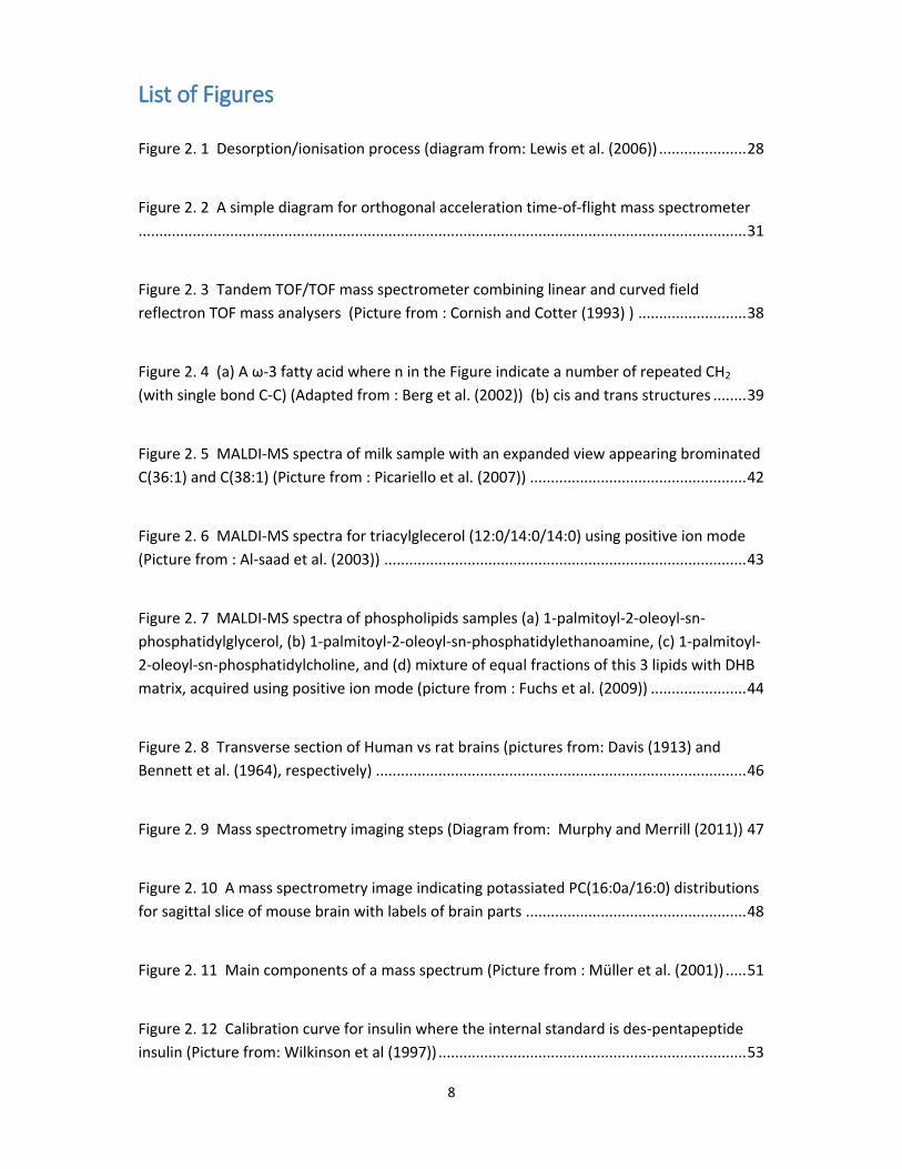
The process of desorption/ionisation is illustrated in Figure 2.1. When a laser beam
hits the sample-matrix substance deposited on a target, some fraction of energy is absorbed
by the matrix and corresponding sample molecules. The absorbed energy, 𝐸𝑎 into affected
sample volume, 𝑉 (determined by spot size and penetration depth of beam into the
sample), can be expressed in term of laser fluence as follows.
𝐸𝑎
𝑉 = 𝛼𝐻 (2.2)

28
Where laser fluence, 𝐻 which is defined as energy per unit area at depth, 𝑧 from sample
surface decays exponentially as a function of 𝑧 as shown in equation (2.3) (Hillenkamp et al.,
2013) .
𝐻 = 𝐻0𝑒−𝛼𝑧 (2.3)
With 𝐻0 being the fluence at 𝑧 = 0 and 𝛼 being absorption coefficient of sample-matrix at a
specific laser wavelength (Hillenkamp et al., 2013). Therefore, by integrating equation (2.3),
equation (2.2) is obtained.
Figure 2. 1 Desorption/ionisation process (diagram from: Lewis et al. (2006))
As a co-crystallised structure is formed between molecules of the matrix and the
sample, energy absorbed by matrix molecules is released to sample molecules via thermal
desorption (Hillenkamp et al., 2013). Whilst escaping the sample surface, the matrix
molecules evaporate from sample-matrix clusters and hence ionisation of some sample
molecules as seen in Figure 2.1. However, the majority of energetic sample molecules are
non-ionised and leave the sample source as neutrals. An Einzel lens brings a divergent ion
beam into focus. The ion beam experiences electric field as passing through a series of
component lenses, causing the ion beam to diverge and re-focus (Sise et al., 2005).
Few kV
Sample-matrix plume
Ions
Sample
-matrix
crystals Laser pulse

29
2.2.3 Ion Acceleration
The very first ion accelerator for TOF-MS applications dates back to a simple two-
plate capacitor (Stephens, 1946; Cameron and Eggers, 1948; Wolff and Stephens, 1953).
Where voltage is applied between the two parallel plates resulting in acceleration of ions
produced between the plates is built up. The ion potential energy changes when and electric
field is applied. The sum of the potential energy and the initial energy obtained from
ionisation procedure (left hand side of equation (2.4)) will be fully turned into kinetic energy
(right hand side of equation (2.4)) after leaving an exit grid of the accelerator into the mass
analyser, following the law of conservation of energy.
𝑞𝑉 + 𝑈0 = 1
2𝑚𝑣2 (2.4)
Where 𝑞 is ion charge, 𝑉 is electric potential different at the ion source (typically 20 kV), 𝑚
is ion mass, 𝑣 is speed of ion when leaving electric field and 𝑈0 is an initial energy after
ionisation (translational energy).
However, individual molecules with identical mass-to-charge ratio are rarely ionised
at exactly the same time or distance, nor do they carry the same momenta. There exists
some shift in flight-time measurements from ion to ion even though their masses are equal.
Spatial differences at which the ions are formed, transforms to a kinetic energy distribution
of ions in the mass analyser (drift) region which expands the flight-time distribution (see
more details in Section 2.2.4). Applying the Newton’s second law of motion, equation (2.5)
determines a value for acceleration in the accelerating region.
𝒂 = 𝑞𝑬
𝑚 (2.5)
Where 𝒂 is acceleration in the electric field direction and 𝑬 is electric field.
Accordingly, the time an ion takes to leave the acceleration region, 𝑡𝑎′ is given by
equation (2.6) (Guilhaus, 1995). Assuming that sample molecules are ionised in the same
plane relative to the electric field direction.
𝑡𝑎′ = −
√2𝑚𝑈0
𝐸𝑞 ±
√2𝑚(𝑈0+𝐸𝑞𝑠)
𝐸𝑞 (2.6)

30
Where 𝑠 is a displacement of ion while being accelerated (only the displacement along the
axis of accelerating field is important). Given that the direction of acceleration is positive.
Hence, the sign of 𝑡𝑎′ indicates whether the direction of ion’s initial velocity is the same as
that of acceleration. In other words, positive valued 𝑡𝑎′ s refer to ions that continue to travel
in the same direction as their initial velocity. On the other hand, those with negative values
mean that their initial velocities oppose the accelerating field. So they undergo deceleration
prior to acceleration which results in change in trajectory direction and would take some
extra time over the ones with same initial energy but initially travel downstream. In reality,
the time an ion spends in acceleration region, 𝑡𝑎 = |𝑡𝑎′ |. Where two times the first term of
equation (2.6) is known as the turn-around time an opposing ion needs to catch up its
original position that often occurs in ionisation events (Guilhaus, 1995).
Space focus is arranged such that ions with different kinetic energies are spreading
over smallest possible displacement along acceleration field. This removes the spatial and
energy shifts up to some extend which leads to improvement of the overall flight-time
resolution. Furthermore, the even better temporal resolutions can be achieved via
additional energy correction steps (see Section 2.2.6).
2.2.4 The Time-of-flight Mass Analyser
MALDI-MS is usually coupled with a time-of-flight mass analyser. Other types of
mass analysers such as quadrupole, ion cyclotron resonance are also available but are less
commonly built for commercial purposes. The reasons that have made time-of-flight
instrument a major mass analyser for MALDI-MS is that it is designed to detect pulsed ions
with ideally no limit in mass range. Also, TOF with a subsequent mass analyser of same or
other types can be constructed to perform multiple MS analysis. Therefore, in this
instrumental design part, only the MALDI-TOF-MS instrument as the main type of MALDI-
MS is focused.
In time-of-flight instruments, flight-time is a parameter to be quantified and
converted into mass information. The total flight-time can be expressed as overall times
spent in acceleration region, 𝑡𝑎, drift region, 𝑡𝐷 and also any delayed time during ionisation
and detection processes.

31
The time-of-flight mass analyser is a simple yet effective tool for determining ion
masses. Charged particles from the ion source are accelerated through an appropriated
path inside the mass spectrometer. The time taken to reach the detector called “time-of-
flight” or “flight-time” is the only main parameter to be measured. Suitable detectors can
measure the flight-time of ion packets with different masses. This information is then
passed for computer processing to obtain mass spectra (intensity vs. m/z).
Linear Time-of-flight Mass Spectrometer
An ion enters the drift region of length, 𝐷 with a final velocity from the accelerator
that can be worked out from equation (2.4) of conservation of energy. The ion exerts no
force in the vacuum drift region. It therefore travels with the constant velocity throughout
the drift region. The time it takes to pass the drift region, 𝑡𝐷 is derived in equation (2.7).
𝑡𝐷 = 𝐷
2√
2𝑚
(𝑈0+𝑞𝐸𝑠) (2.7)
From equations (2.6) and (2.7), the total flight-time, 𝑡 is directly proportional to the square
root of mass (𝑡 ∝ 𝑚1
2). Finally, the ion beam hits a detector device which generates a signal
from which the distribution of time-of-flight times of the different mass ion in the beam is
calculated. A diagram for this type of mass spectrometer is shown in Figure 2.2.
Figure 2. 2 A simple diagram for orthogonal acceleration time-of-flight mass spectrometer (Picture from : Fjeldsted (2003))
Accelerating region Flight path distance (D)
Drift region Ion
optics
Ion source
Detector

32
In this simplest time-of-flight mass spectrometer, there is a limitation due to the fact
that ions are created in slightly different locations in space as mentioned earlier in Section
2.2.3. The spatial variation of ions in the direction of electric field affects velocities and
therefore the flight-time of ions of the same mass-to-charge ratio leaving the exit plate of
the capacitor. Each ion with the same mass and carrying equal charge is accelerated at the
same rate in the static electric field between the capacitor plates, as described in equation
(2.5). The potential difference in static electric field varies as a function of distance to be
accelerated. Thus, the final velocity of same ion varies as a function of distance being
accelerated within the capacitor as a result of differences in kinetic energy. These cause
time-of-flight mass peaks in spectra to broaden influencing the mass resolution (see Section
2.2.6 for the definition of mass resolution). The uses of linear and curved field reflectrons
are approaches to overcome this distribution of flight times.
Reflectron Time-of-flight Mass Spectrometer
The reflectron also known as the ion mirror, reflects the incoming ions causing them
to travel the opposite direction to the initial direction. It makes use of electrostatic lens
components which create a retarding electric field gradient.
Ions with identical mass-to-charge ratio in the drift region have a small kinetic
energy distribution caused mostly by initial energy when ions are formed. The longer the
flight path, the more significant shift in flight-time of these same ions would be observed as
a result of their variation in velocity. Higher velocity ions have a relatively short flight-time in
the drift region compared to lower velocity ions. To reduce the flight-time shift, these ions
must be introduced into a reflectron (Cornish and Cotter, 1993). The reflectron’s electric
field decelerates the ions when they are travelling inbound until they stop, then
reaccelerates them in the outbound direction (Cornish and Cotter, 1993). Faster ions spend
more time in the reflectron region as they penetrate slightly deeper than slower ones, this
corrects for different time spent in the drift region. Also, a focus is made at the point where
the ion packet is most compressed (in time). The results indicate far better mass resolving
power than linear instruments with same drift length. It therefore gives high performance
without the need to build larger mass spectrometers.

33
Curved Field Reflectron Mass Spectrometer
Curved Field Reflectron (CFR) is a subsequent generation of reflectron developed by
Cotter and Cornish (1993). This aims specifically to remove imperfections in MS/MS Time-of-
flight mass analysis. When ions are fragmented via collision induced dissociation (CID), the
kinetic energy of product ions depend solely on their mass, leading to separations of focal
points associated with the depth travelled by ions into a linear reflectron as from SIMION
trajectory simulations (Cornish and Cotter, 1993). In contrast, a curved field reflectron
incrementally reduces the strength of the electric field as it goes deeper into the reflectron.
In other words, the potential used to create the field goes down at a constant rate with the
form of “the arc of a circle” to satisfy conditions determined by SIMION simulations (Cornish
and Cotter, 1993). Thus, the focal points of different products (and their parent) ions are
brought focused more tightly than with the linear reflectron.
2.2.5 Detector
The detection system includes the ion detector, signal amplifier and signal
acquisition electronics. The output of ion signal vs. mass-dependent flight-time variations of
ions is recorded and turned into a mass spectrum. A microchannel plate (MCP) detector is
often used as an ion detector in MALDI-TOF-MS instruments. An incident ion collides with
the detection surface and activates secondary electrons in parallel electron multiplier tubes
of few micrometers diameter in order to amplify signals.
At a certain kinetic energy, ions with higher masses will travel with lower velocities
which might not be sufficient for secondary electron emission to occur and can result in a
decay of MCP detection sensitivity. For example, the detection of immunoglobulin G (IgG)
dimer and whose mass is about 300 kDa can be more than 10% less sensitive than the
detection of the 1 kDa angiotensin ion (Liu et al., 2014). If ions are accelerated with higher
voltage, the kinetic energy and therefore velocity of all ions increase and the sensitivity is
then improved. On the other hand, detection of fast moving, high incident energy ions
might be limited by the saturation of the detector which can give rise to a poorer resolution.
Temporal resolution can currently be detected down to the order of nanosecond or less (Li
and Whittal, 2009). In addition to the conventional approach, Ion conversion detector (ICD)
and superconducting tunnel junction (STJ) are attempts to overcome this sensitivity

34
limitations as velocity-dependence no longer applies (Wenzel et al., 2006). Also, high
sensitivity can be attained by increasing detector voltage, however, would raise the level of
electrical background noise at the detector and lead to a corresponding reduction of signal-
to-noise (Wetzel et al., 2006).
2.2.6 Mass Resolution
The mass resolution is defined by equation (2.8).
𝑚𝑎𝑠𝑠 𝑟𝑒𝑠𝑜𝑙𝑢𝑡𝑖𝑜𝑛 = 𝑚
∆𝑚 (2.8)
Where ∆𝑚 is width of the mass peak for mass, 𝑚 in the spectra (sometimes width values at
full width half maximum or at 10% of the peak height is used). ∆𝑚 represents how much the
mass measurements are distributed for that peak. And the mass resolution represents an
ability to tell apart different peaks in a mass spectrum.
Mass resolution can be calculated from the resolution of flight-time which is a direct
measurement of time-of-flight instruments as the 𝑡 ∝ 𝑚1
2 relation is known. Flight-time is
approximately equal to drift time providing that accelerating time is much smaller than drift
time (𝑡𝑎 ≪ 𝑡𝐷). Therefore, mass resolution can also be derived using equation (2.7) and its
derivative with respect to 𝑈0. In addition, potential energy caused by accelerating an ion
through the electric field dominates the initial translational energy (𝑈0 ≪ 𝑞𝑉) such that 𝑈0
can be ignore. Therefore, the mass resolution for time-of-flight mass spectrometer is
estimated as in equation (2.9) in terms of flight-time and internal energy, respectively.
𝑚
∆𝑚=
𝑡
2∆𝑡=
𝑈0+𝑞𝑉
∆𝑈0 ≈
𝑞𝑉
∆𝑈0 (2.9)
Note that the electric field is in fact not perfectly uniform.
Further improvements of space focus in the acceleration region, include placing
another electric field next to the initial space focus field following an instrument designed
by Wiley and McLaren (1955), taking into account appropriate ratios of the two electric field
strengths and acceleration distances (Weinkauf et al., 1989; Karas, 1997). These designs
eliminate up to the first and the second terms of equation (2.10) of Taylor’s expansion
which express the inverse flight-time resolution as a function of kinetic energy distribution,

35
respectively (Weickhardt et al., 1996). The results predict a much better mass resolution
compared to the single field design (see Section 2.2.3) without having to extend too far the
space focus distance.
∆𝑡
𝑡= 𝑎
∆𝑈
𝑈+ 𝑏 (
∆𝑈
𝑈)
2+ 𝑐 (
∆𝑈
𝑈)
3+ ⋯ (2.10)
Where 𝑡 is the overall flight-time, 𝑈 is the ion’s kinetic energy and 𝑎, 𝑏, 𝑐 are constants.
The arrangements of linear and curved field reflectrons as discussed in Section 2.2.4
that lead to better flight-time focus would offer similar improvements in temporal
resolution.
2.2.7 MALDI Matrices
The matrix is the core to the process of MALDI as described in Section 2.2.1. A matrix
is selected such that sample-matrix crystals are formed properly and suits an experiment.
Standard matrices for MALDI-MS of biological molecules include α-cyano-4-hydroxycinnamic
acid (CHCA), dihydroxybenzoic acid (DHB) and sinapinic acid (SA). They are able to absorb
energy from ultraviolet frequency lasers. The structure of the ions created from samples
with the use of DHB matrix are more preserved compared to ones with CHCA matrix which
normally causes significant degradation (Hazama et al., 2008). Therefore, CHCA matrix is
well-suited for analytes of lower mass range whereas DHB as well as SA can be used with
higher mass range to avoid fragmentations.
The more acidic a matrix is, the better positive ion yields are obtained (Schiller et al.,
2007; Dashtiev et al., 2007). Additional trifluoroacetic acid (TFA) could enhance signal-to-
noise ratios of mass spectra (Damnjanovic et al., 2011). DHB is used as a matrix to prepare
most lipid samples, especially the 2,5-DHB type which gives the best quality mass spectra of
all the isomers, as a result of relatively high positive ion yield and small crystal size relative
to other available types, i.e. 2,3-DHB, 2,4-DHB, 2,6-DHB, 3,4-DHB and 3,5-DHB (Schiller et
al., 2007).
It is possible to make up a matrix compound of more than one component. For
example, DHB/CHCA as reported in Laugesen and Roepstorff (2003) could combine the
advantages of reproducibility from CHCA and tolerance to contaminations from DHB.

36
2.2.8 Sample Preparation (Sample-matrix Depositions)
Appropriate matrix type and sample preparation methods are selected for each
analyte and objective of analysis. Where optimal mass accuracy, resolution and
reproducibility with appropriate signal intensity are desired in each MALDI-MS experiment.
In general, a sample should be prepared in suitable conditions to form significant numbers
of analyte-containing matrix crystals. Such crystals should distribute homogeneously
throughout its drop on a sample target with uniform shape and alignment. Also, the target
supporting the sample must be cleaned properly to minimise impurities. Optional
purification methods of hydration/recrystallisation or sublimation/recrystallisation (Yang
and Caprioli, 2011) can be used. Contaminants that are highly soluble in water will be
dissolved and can be removed, and the remaining, purer crystals stick on the target plate.
Solvents are added to turn crystals back to the original sample-matrix solution in order to
allow reconstruction of crystals.
The original dried-droplet sample preparation method is achieved by spotting matrix
solution on top of wet sample solution spotted earlier on a metal target, then let dry.
Another approach can be making a mixture of saturated matrix and sample solutions, then a
small droplet of this is spotted onto a metal target. The dried-droplet technique results in
large crystal sizes which can be found quite separate to contaminants at some specific
points on the target. Therefore, useful spectra can be repeatedly gained from those large
crystals at selected spatial locations. MALDI targets are usually designed to hold several
sample droplets that can be conveniently analysed in the same session.
The homogeneity of the MALDI sample surface depends on size of the crystals being
formed which is affected by type of matrix, analyte concentrations and could be improved
by selecting a solvent with high evaporation rate. A matrix solution is deposited and dried
on the target plate before finishing the above layer with a sample solution. Crystals formed
by this method are relatively small in size. Better homogeneity of the preparation is
achieved this way but limited spectra per crystal are produced. To minimise this
disadvantage, the dried-droplet can be applied on top of this preparation to accrete the size
of the existing crystals.

37
2.2.9 Tandem Mass Spectrometry
A tandem mass spectrometry system refers to the use of two or more mass
analysers each subsequently perform mass spectrometry analysis. Usually 2 mass analysers
are used, call this method MS/MS or MS2. Between 2 consecutive analysers, there is a
collision chamber containing neutral gas, usually helium, argon and nitrogen. Collision with
neutral gas molecules can fragment a parent ion (Wells and McLuckey, 2005). The process is
called collision induced dissociation (CID). More fragmentations were found when target gas
of heavier molecular weight was used, providing high centre-of-mass collision energy
(Bordas-nagy et al., 1992). The purpose of tandem MS is to extract structural information
from the analyte. First of all, analytes’ m/z(s) in the mixture (within a defined mass range)
need to be identified in order to make a selection on the interested one. This can be done
using the ion mass spectra resulted from the first mass analyser by gating narrower mass
range that covers appropriate mass peak of a particular m/z. Only ions with the selected
mass range called precursor ions undergo decomposition into product ions and suffer
neutral losses. These product ions then go on to the second mass analyser for further mass
analysis. The mass spectra of product ions illustrate the masses of components within the
precursor (parent) ions. Alternatively, MS/MS spectra of the whole mass range can be
scanned to observe a specific product ions resulting from CID and metastable decays which
could indicate the possible precursor of that class. For increased selectivity and sensitivity,
selected reaction monitoring (SRM) is performed at specific precursor’s and product’s m/z
values (Lange et al., 2008). The other method called neutral loss scan is also applicable by
observing for a specific interval between mass peaks, then all possible products of a
precursor can be determined and vice versa.
An early tandem MS instrument is a magnetic/electric sector. Ions pass 90o magnetic
sector component (constant field) followed by scanning electric field in the 90o electrostatic
sector where the mass of product ions are determined based on their kinetic energy
(Beynon et al., 1973). This paved the way for generations of MS/MS instruments. Accurate
measurements can be achieved with triple quadrupole (Yost and Enke, 1979) and FT-ICR
instruments, both select precursor ions precisely using coherent RF waves. Not only space
separated tandem mass spectrometry using multiple mass analysers, but also time
separated tandem mass spectrometry using ion traps can be performed (Payne and Glish,
2005). Tandem mass spectrometry based on TOF/TOF instrument is another fast improving

38
method due to its simplicity, robustness and wide mass range. The correction for the
varying focal length of different mass ions was solved by Cornish and Cotter (1993) who
developed the curved field reflectron as discussed in section 2.1.4. A diagram for this design
of tandem reflectron TOF MS/MS is illustrated in Figure 2.3.
Figure 2. 3 Tandem TOF/TOF mass spectrometer combining linear and curved field reflectron TOF mass analysers (Picture from : Cornish and Cotter (1993) )
Note that hybrid systems that combine different types of analysers are also available such as
sector/quadrupole, sector/TOF and the commercially most abundant quadrupole/TOF (Glish
and Burinsky, 2008).
2.2.10 MALDI-MS Imaging
Mass spectrometry imaging (MSI) allows MS information to be represented as an
image, mapping distribution of analytes in each of its pixels in correspondence to the spatial
positions on the actual sample. Hence, applications can be in structural observations of
biological molecule distributions in tissues and their change due to pathological conditions.
A simple microprobe MSI controls the trajectory of laser beam relative to spatial
coordinates of the plane of sample being acquired either by moving the laser beam across
the sample area, or vice versa. Series of mass spectra at each known point in space are
recorded. The size of the focusing beam influences the spatial precision (McDonnell and
Heeren, 2007). In contrast, microscope type MSI collects both MS and spatial coordinates
data at a position-sensitive detector. This allows measurement without the need to
determine the location at which each MS spectrum is acquired in the initial stage. The
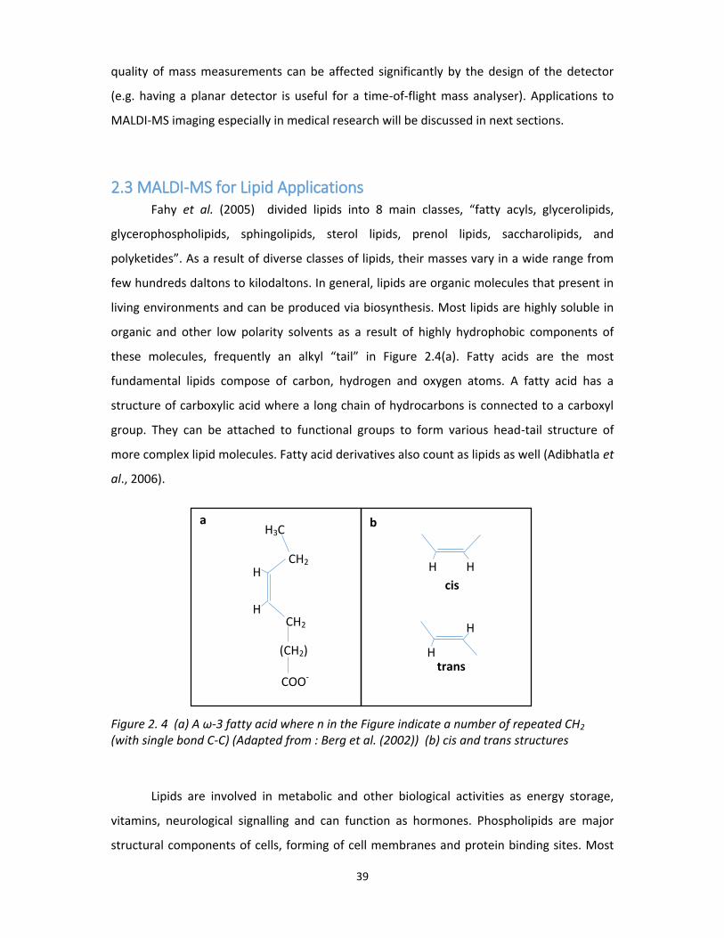
39
quality of mass measurements can be affected significantly by the design of the detector
(e.g. having a planar detector is useful for a time-of-flight mass analyser). Applications to
MALDI-MS imaging especially in medical research will be discussed in next sections.
2.3 MALDI-MS for Lipid Applications Fahy et al. (2005) divided lipids into 8 main classes, “fatty acyls, glycerolipids,
glycerophospholipids, sphingolipids, sterol lipids, prenol lipids, saccharolipids, and
polyketides”. As a result of diverse classes of lipids, their masses vary in a wide range from
few hundreds daltons to kilodaltons. In general, lipids are organic molecules that present in
living environments and can be produced via biosynthesis. Most lipids are highly soluble in
organic and other low polarity solvents as a result of highly hydrophobic components of
these molecules, frequently an alkyl “tail” in Figure 2.4(a). Fatty acids are the most
fundamental lipids compose of carbon, hydrogen and oxygen atoms. A fatty acid has a
structure of carboxylic acid where a long chain of hydrocarbons is connected to a carboxyl
group. They can be attached to functional groups to form various head-tail structure of
more complex lipid molecules. Fatty acid derivatives also count as lipids as well (Adibhatla et
al., 2006).
Figure 2. 4 (a) A ω-3 fatty acid where n in the Figure indicate a number of repeated CH2 (with single bond C-C) (Adapted from : Berg et al. (2002)) (b) cis and trans structures
Lipids are involved in metabolic and other biological activities as energy storage,
vitamins, neurological signalling and can function as hormones. Phospholipids are major
structural components of cells, forming of cell membranes and protein binding sites. Most
H3C
CH2 H
H CH2
(CH2)
n COO-
a
H H
cis
b
H
H
trans
s

40
biological cell membranes largely consist of phosphatidylcholine (PC). Normal cells have
different lipid components and distributions at specific organelles and cell types (van Meer
et al., 2008). Hence, abnormal changes of lipid distributions might be good indicators for
some pathological disorders. There are attempts to produce quantitative studies of lipids to
possibly trace lipid metabolism in cancer tissues that could identify cellular activities stated
as hallmarks of cancers (Hanahan and Weinberg, 2000; 2011; Santos and Schulze, 2012). As
brain tissues are lipid-rich, observing for the correlations between lipid concentrations and
brain diseases, disorders and damage has become an interesting topic of research
(Adibhatla et al., 2006).
2.3.1 Lipid Extraction Techniques
An extraction method using chloroform and methanol has been used in several
applications due to its simplicity and robustness. Chloroform, methanol and deionised water
in an appropriate ratio can be added to a biological compound to allow lipid extraction with
no need to heat or evaporate the sample (Bligh and Dyer, 1959). Chloroform and lipids form
a solution that sets itself apart from water, methanol and other polar substances in the
compound which is seen as a separated top layer. This extraction method requires only a
small supply of sample. In comparison with the previous extraction method, rapidity of the
procedure is maintained but the yield and purity of lipid extracts are significantly improved.
Chloroform could be added, followed by adding water to the lipid extracts to repeat
extractions until a satisfactory level of purification is achieved. In tissue sample applications,
the tissue sample could be blended to allow this extraction process or thin slices of tissues
could be acquired using imaging mass spectrometry.
Thin layer chromatography (TLC) is a technique to separate components in the lipid
extracts based on their mass and polarity properties. Lipids move different distances on a
chromatography plate. Note that silica gel is often used as a stationary phase and the
chloroform-methanol mixture is a mobile phase solvent. Furthermore, liquid-solid extraction
can be applied by dissolving sample compound in different solvents of varying polarity and
pH. This allows filtering out the undissolved parts at each step, and hence separation for
different compound classes before introducing into analysis system.

41
2.3.2 Spectral Analysis (in Lipid Classification)
Mass spectrometry is widely used in proteomic studies, but can also be used for
lipidomics. In particular, MALDI is one of the soft ionisation methods that was shown to
generate useful ions for quantitative analysis of a wide mass range of biological molecules.
MALDI-TOF-MS analysis of phospholipids and triacylglycerols by Emerson et al. (2010)
requires as tiny portion as 1 µl of extracted lipids from beef and egg yolk samples. Mass
determination together with structural information can be obtained by performing MS/MS
(MS-MS) or MSn which is very useful to deal with complex lipid molecules.
Lipidomics covers the structural and functional study of lipids in living cells, and their
role in supporting metabolic processes, including interactions between lipids and other
fundamental biomolecules – i.e. generic and protein molecules contained in the cells. There
are 2 main aspects for lipid mass spectrometry analysis. The classical one is when lipid
extracts are separated through appropriate gas or liquid chromatography before being
introduced to a mass spectrometer. This is so-called “comprehensive lipidomics analysis by
separation simplification” (CLASS) allows selected classes of lipids to be analysed by the
mass spectrometer, one at a time (Harkewicz and Dennis, 2011) . Whereas another method
called “shotgun lipidomics” applies ESI mass spectrometry to the lipid extracts directly (Han
and Gross, 2005).
The common shorthand notation for fatty acid (carboxylic acid) isomers can be
written as 𝐶 ∶ 𝐷 representing number of carbon atoms : number double bonds connecting
carbon molecules contained within the structure of the fatty acid molecule. This reduces the
complexity of writing the lipid structure as a standard chemical formula. Molecular
information of complex lipids can be described by quoting each of its fatty acid fraction
along with its head group. For adding clarity if D is non-zero in a fatty acid isomer, the
symbol n-x or 𝜔x is used with the x being the numerical order of the first double carbon-to-
carbon bond as count from its methyl side (Harwood and Scrimgeour, 2007). e.g. an
essential fatty acid, Docosahexaenoic acid (DHA) can be expressed as 22:6 (n-3) means that
it has 22 carbon atoms with 6 double bonds in the carbon chain, the first double bond is at
𝜔3 position. If there is a double bond in the molecule, the fatty acid is said to be non-
saturated; otherwise, it is saturated. Metabolism rates in the organic tissue are thought to
be increased with the degree of phospholipid unsaturation in membrane (Hulbert and Else,

42
1999). The conformation at each double bond could be either “trans” or “cis” as illustrated
in Figure 2.4(b) which are reflected in the properties of lipid molecules such as polarity,
thermal stability. However, current mass spectrometers might not provide enough
information to distinguish between these two.
Typical lipids are saturated and have even number of carbons shown in the mass
spectra in Figure 2.5 of lipid derivatives from a milk sample.
Figure 2. 5 MALDI-MS spectra of milk sample with an expanded view appearing brominated C(36:1) and C(38:1) (Picture from : Picariello et al. (2007))
If the sample is treated with bromine, a brominated lipid would show up in a mass spectrum
as a shift in peak with an additional mass per double bond equal to molecular mass of Br2 of
approximately 160 Da and displaying a bromine isotope pattern (Picariello et al., 2007).
From Figure 2.5, peaks for brominated C(36:1) and C(38:1) are well illustrated. A
determination of double bonds can be done by observing degrees of oxygenation as in a
study of unsaturated oils using MALDI-MS (van den Berg et al., 2004) .

43
Figure 2. 6 MALDI-MS spectra for triacylglecerol (12:0/14:0/14:0) using positive ion mode (Picture from : Al-saad et al. (2003))
Loss of different carboxylate groups in a triacylglycerol (TAG) are equally likely as the
ratio between the positive ion peaks at masses of remaining fragments agrees with the yield
of these carboxylate groups in the lipid – i.e. intensity of the remaining fragment from loss
of C(14:0) is twice as much than loss of C(12:0) following Figure 2.6. Therefore, the relative
intensities of the fragments could determine the relative abundance of each carboxylate
group contained in a molecule (Al-saad et al., 2003).
No MS signals appear at the mass of carboxylate loss might indicate that they are
hydrogenated or salted immediately. Thus, only masses of remaining fragments form
molecular or sodiated ions of molecule, M could present on mass spectra. The only mass
peaks of these remaining fragments are of masses equal to [MH-RCOOH]+ or [MNa-
RCOONa]+ which cannot be distinguished. In case a lipid molecule undergoes sodiation,
there should be possibilities for its carboxylate fragments to be both hydrogenated and
sodiated but there was no evidence of remaining fragment from hydrogenated ones [MNa-
RCOOH]+ shows up on mass spectra (Al-saad et al., 2003). This means prompt
fragmentations from sodiated TAGs are minor compared to the protonated version of same
TAGs.
Phospholipids have a phosphate head group attached to more than one carboxylate
tail. The phosphate groups are the polar part of phospholipids. Again, the prompt

44
fragmentations of polar heads occur with the hydrogenated phospholipids rather than the
greater fraction salted phospholipids.
2.3.3 Limitations and Challenges
In phospholipids, the head group
of phosphatidylcholine (PC) type can
cause severe signal suppression to
fragment ion signals of other head
groups, especially in phosphatidyl-
ethanolamine (PE) which is also
commonly present in biological
compounds (Emerson et al., 2010). Figure
2.7(d) shows suppression effect PC acts
onto PE and phosphatidylglycerol (PG)
fragment ions compared to each
individual spectra in Figure 2.7(a), (b) and
(c) when positive ion mode of MALDI-MS
was used. The negative molecular ions of
PC are not possible to be detected using
MALDI-MS (Al-saad et al., 2003). The
negative ion mode is then favoured for a
detection of PE and PG which is normally
suppressed by the PC in positive mode
arrangements. Para-nitroaniline (PNA) as
a matrix substance would give non-acidic
environment that enhance the detection
of the negative molecular PE ions (Fuchs et al., 2009).
Matrix and analyte suppression effects occur in the presence of significant amounts
of salts as they also catch positive charges (Lou et al., 2009). In MALDI-MS experiments,
alkali metal salts of proteins were washed after depositing samples onto a target in order to
minimise the chemical background noises they caused (Smirnov et al., 2004). This might be
applicable to remove lipid salts as well.
a
b
c
d
Figure 2. 7 MALDI-MS spectra of phospholipids samples (a) 1-palmitoyl-2-oleoyl-sn-
phosphatidylglycerol, (b) 1-palmitoyl-2-oleoyl-sn-phosphatidylethanoamine, (c) 1-palmitoyl-2-oleoyl-sn-phosphatidylcholine, and (d) mixture
of equal fractions of this 3 lipids with DHB matrix, acquired using positive ion mode
(picture from : Fuchs et al. (2009))

45
Nowadays, interest in lipodomics seems to be growing as lipid metabolism can
diagnose cellular dysfunctions. However, due to the complexity of lipid analyses, there is
relatively little research leading to a lower availability of lipidomic databases compared to
that of proteomics. There are many classes of lipid which occupy a wide mass range and the
MS analysis is particularly limited at high masses. However, mass spectrometry technology
is continuously evolving. MS/MS analysis of lipids with a mass resolution of greater than
30,000 can be achieved using a quadrupole mass analyser to select lipids at an increment of
1 Da to pass to a CID system and then proceed through a time-of-flight mass analyser for
final mass analysis (Simons et al., 2011). The “Lipidomic Gateway” website
(http://www.lipidmaps.org/) is a good resource for lipid identification whose information is
based on lipid classification studies as updated in 2009 by Fahy and coworkers which
provides a database of lipid structures and MS peaks of all lipid classes. This has been
reviewed every year. Nevertheless, numerous subclasses of hydrocarbon chains and
bonding could cause a lot of confusion to mass spectral analysis of large lipids (Fahy et al.,
2005). Therefore, careful TLC or gas chromatography separation methods is needed for full
resolution.
2.3.4 Lipids in the Brain
As discussed earlier, a variety of lipids are found in biological cells as structural and
functional components. Brain tissues in general have very high lipid concentrations. Lipid
types and distributions should be consistent in normal brains as required to perform proper
activities. Therefore, unusually distributed lipids in some parts of the brain may link strongly
to diseases, disorders and damage. Quantitative imaging is therefore a powerful tool to
investigate this kind of anatomical pathology giving biochemical composition as well as
anatomical information. MALDI imaging is particularly useful in detecting intact large
molecules like lipids at precisely determined spatial locations.
There are similarities between human and rat brains that make a rat brain a
reasonable model for the study of brain disorders relevant to humans. In the 1960s (Bayer
et al., 1993) confirmed that human and rat brains show very close correlation in processes
of central nervous system (brain and spinal cord) development since their embryonic stages.
Where same developmental stage occurs in the same order but at different time scales.
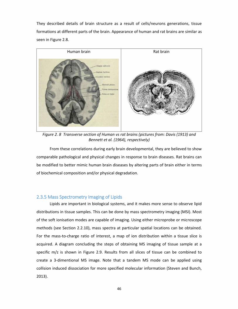
46
They described details of brain structure as a result of cells/neurons generations, tissue
formations at different parts of the brain. Appearance of human and rat brains are similar as
seen in Figure 2.8.
Human brain Rat brain
Figure 2. 8 Transverse section of Human vs rat brains (pictures from: Davis (1913) and Bennett et al. (1964), respectively)
From these correlations during early brain developmental, they are believed to show
comparable pathological and physical changes in response to brain diseases. Rat brains can
be modified to better mimic human brain diseases by altering parts of brain either in terms
of biochemical composition and/or physical degradation.
2.3.5 Mass Spectrometry Imaging of Lipids
Lipids are important in biological systems, and it makes more sense to observe lipid
distributions in tissue samples. This can be done by mass spectrometry imaging (MSI). Most
of the soft ionisation modes are capable of imaging. Using either microprobe or microscope
methods (see Section 2.2.10), mass spectra at particular spatial locations can be obtained.
For the mass-to-charge ratio of interest, a map of ion distribution within a tissue slice is
acquired. A diagram concluding the steps of obtaining MS imaging of tissue sample at a
specific m/z is shown in Figure 2.9. Results from all slices of tissue can be combined to
create a 3-dimentional MS image. Note that a tandem MS mode can be applied using
collision induced dissociation for more specified molecular information (Steven and Bunch,
2013).

47
Figure 2. 9 Mass spectrometry imaging steps (Diagram from: Murphy and Merrill (2011))
Matrix must be carefully deposited such that the matrix would spread out evenly over the
sample either using TLC sprayers, inkjet printers, airbrushes, oscillating capillary nebulisers
or sublimation methods (Zaima et al., 2010), or other, purpose designed instrumentation.
A MSI study of rat’s spinal cord by desorption electrospray ionization MS/MS shows
the expected shape of gray and white matter and the relative local concentrations of lipids
and free fatty acids with spatial resolution of <200 µm (Girod et al., 2010). Mouse’s brain
contains significant lipid concentrations with the main types being phospholipids,
sphingolipids and glycerolipids (Murphy et al., 2009). Murphy et al. (2009) observed
concentrations of potassiated PC(16:0a/16:0) to vary from pixel to pixel over the tissue
section. The quantitative representation of the PC distribution by relative intensity level of
each pixel in the MSI image at m/z 772.5 is seen in Figure 2.10.

48
Figure 2. 10 A mass spectrometry image indicating potassiated PC(16:0a/16:0) distributions for sagittal slice of mouse brain with labels of brain parts
(picture from : Murphy et al. (2009))
Deterioration of the brain can lead to various diseases which decrease capabilities to
carry out usual lipid metabolism at specific brain regions (Adibhatla et al., 2006). Lipid MSI
analysis can be performed at a target brain region to trace for the abnormalities.
Alzheimer’s disease (AD) is a common brain diseases in the elderly which can cause serious
neurodegeneration. It induces abnormal lipid metabolism in the central nervous system at
which quite a lot of lipids in tissues are involved in neurotransmission. Neurotransmission
pathways could yield better understanding of the physiology and pathology with respect to
the anatomical structure. However, the accuracy of the spatial mapping is subject to
resolution. Veloso et al. (2011) carried out research on real human brain samples and
studied particularly the lipid distributions of the central nervous system. The hippocampus is
a part in the central nervous system (located at the prosencephalon of the brain) one of the
primary sites attacked by Alzheimer’s (Mu and Gage, 2011). For hippocampus MSI, to 100
µm imaging resolution was required due to the complexity of the structure (Veloso et al.,
2011). The spatial resolution required determines the number of scans per dimension.
49
2.4 Overview of Quantitative Spectral Analysis
2.4.1 Supporting Software for Mass Spectrometry
The MALDI-TOF-MS instrument used at the Wolfson Molecular Imaging Centre
(WMIC), the University of Manchester is an Axima CFR2+ ToF2 model from Kratos (a
Shimadzu group company) this instrument has been upgraded to have a 1 kHZ laser,
effectively making it equivalent to the more recent “Axima Performance” instrument.
Therefore, in this report this instrument will be called the “Axima Performance MALDI- ToF2-
MS” or “AXIMA” for short. The manufacturer’s “Launchpad” software allows selection of
positive-negative ion, linear-reflectron, MS-MS/MS, MSI modes with ranges of parameter
adjustments, including laser properties, mass range, data processing properties, etc. These
primary set-ups allow the users to perform a variety of experiments and to acquire the
optimised data with the selected sample-matrix types. However, the results can be
optimised in both experimental and data analysis processes with support of other related
software. Furthermore, semi-automated corrections of mass spectra is possible with the
aids of coding.
SIMION is software developed for ion optics simulating with its main applications in
mass spectrometry. It allows calculation of ion trajectory associated with electric field in 3-
dimentional definition. Thus, the nature of incoming ions and electrical devices are
important parameters. Don McGilvery was a pioneer for establishing SIMION as mentioned
in Dahl (2000). He wrote the first version of this as a Fortran-based software in 1973 to solve
for ion behaviour throughout optical devices that could answer the problems he came
across when constructing a double quadrupole mass spectrometer (Dahl, 2000). In 1985,
David Dahl was successful in publishing a personal computer version of this software which
leads to development of subsequence versions with graphics user interface (GUI) (Dahl,
2000). In time-of-flight mass spectrometry applications, SIMION as mentioned in Section
2.1.4 is used to compute voltage increments in the ion mirror in curved field reflectron TOF-
MS. It is used as well to simulate ion trajectory parameters following voltage alterations of
electrodes in the ion source where ion optics are great part in ion focusing and accelerating
systems. Current versions of the software enable collision induced dissociation and taking
into account the repulsion forces between ions (Dahl, 2000; http://simion.com/). Hence,
SIMION is a powerful tool in obtaining accurate calculations for flight-time, flight path
50
coordinates, visualising and keeping records of simulated graphics and data. The increase in
understanding of instruments provided by simulation should improve the resolution and
signal-to-noise when suitable alterations of the apparatus are applied.
MATLAB is a widely used software for statistical and data analysis. As a high-level
programming language, it allows simple coding. Also, it is convenient and easy to handling
and access data. It can be designed to suit personal demands with the ability to create GUI
format programs. Moreover, MATLAB has special sets of built-in algorithms called the
“bioinformatics toolbox” which provides several useful functions to improve spectral
analysis such as baseline subtraction, peak detection, etc., and the “image analysis toolbox”
which can be applied for MS imaging (http://uk.mathworks.com/products/bioinfo/;
White et al., 2005). In mass spectrometry imaging applications, mass spectral data match
spatial voxels to form graphical images of signal distribution throughout the sample (Parry
et al., 2013).
2.4.2 Quantitative MALDI-MS Analysis
Quantitative analyses using MALDI-MS are difficult due to high variability of ion
currents which causes uncertainties in measuring abundance of mass-to-charge information
in mass spectra. The variabilities are subject to the availability of ions in individual
acquisitions which vary between different sample depositions under what are apparently
the same conditions. Ion currents also vary between spatial locations within same sample
deposition well as a result of the non-uniform spread of sample-matrix crystals, and even
shot-to-shot changes at exactly the same position as ablation occurs when the laser is fired
(Duncan et al., 2008). Huge differences are of course contributed by different sample/matrix
preparation and deposition methods, as discussed in Sections 2.2.7 and 2.2.8. These are the
significant influences that limit repeatability in MALDI-MS experiments. Mass
spectrometrists have been seeking methods which could provide more meaningful
quantitation in MALDI-MS analysis. Approaches that yield significant improvement in
MALDI-MS quantitation include those that compensate for both physical and chemical
variabilities of the processes and should overcome some of the systematic and random
errors. Techniques are being investigated based on approaches to sample preparation,

51
instrumentation, calibration using internal and external standards, and mathematical
approaches to data processing and analysis.
An effective temperature of the plume in an early stage of ionisation is one of the
parameters which influences ion yield during an ionisation event (Bae et al., 2013). Where
the ratio of the fraction of protonated analyte yield to the fraction of protonated matrix
yield, is known to correspond only to an early effective temperature of the plume. This is
because the positive charges from the protonated matrix is transferred in order to ionise
the neighbouring analyte molecule during the desorption/ionisation process. Moreover, Bae
et al. (2013) appear to find that by keeping the plume temperature constant during the
desorption/ionisation process, they should improve the consistency of ion abundance.
The heterogeneities of crystal formation also influence the variance of signal
intensity. This causes lower signal-to-noise values in regions where there are fewer crystals.
In contrast, the optimum signal intensity obtained from a crystalline region might result in
saturation of the mass spectra. An automated system can be used to select only the spectra
with appropriate quality- i.e. a spectrum acquired from a single laser shot which has a
satisfied level of signal-to-noise yet saturated (Duncan et al., 2008). A collection of these
mass spectra that pass predefined thresholds are allowed to proceed into the average or
accumulative forms.
Figure 2. 11 Main components of a mass spectrum (Picture from : Müller et al. (2001))
Figure 2.11 illustrates the main components of a mass spectrum. The peaks represent the
associated m/z values of each composition of the experimental sample that has been

52
detected. The peak’s height or relative signal intensity is determined from the ion current.
Noise is always generated along with every acquisition, possibly due to chemical and/or
instrumental, background fluctuations. This can cause random interference to useful signals
which affect the ability to quantify. Müller et al.(2001) defined the signal-to-noise ratio to
be
Signal/noise = 2.5 ×𝑆𝐻−0.5𝑁𝑝𝑝
𝑁𝑝𝑝 (2.11)
Where 𝑆𝐻 is the height of central intensity of a peak measured from the lower boundary of
noise and 𝑁𝑝𝑝 is peak-to-peak amplitude of noise as illustrated in the expanding view of the
Figure 2.11 mass spectrum measured from the lowest to the highest levels of noise.
An internal standard is a selected substance of known concentration added to and
uniformly distributed in the sample under analysis in order to improve quantitative accuracy
of an analyte of interest. A good internal standard should have properties as close to the
analyte as possible, allowing them to behave like the original molecules and participate in
same desorption/ionisation events to the analyte but would represent different mass-to-
charge peak in the mass spectrum. This is most often achieved using isotopically labelled
analyte molecules, where available. A linear relationship is expected between the signal
intensity of analyte to internal standard and the analyte concentration, seen as the
calibration curve in Figure 2.12, given that other experimental conditions are fixed. Hence,
yielding predictive values of analyte concentration when the analyte/internal standard peak
intensity ratio is measured. The signal-to-noise was observed to increase with an analyte
concentration (Wilkinson et al., 1997). According to Wilkinson et al. (1997), two main
choices of method can be applied for spectral intensity measurements: 1) linearly average
the noise intensity selected from the main informative part of the mass spectrum, eliminate
the averaged noise, and obtain peak intensity via integration, and 2) use the least squares
method to fit a local package of spectral peaks at each molecular mass including the
protonated molecular ions, dehydrated molecular ions, and might include metastable decay
products and salted molecular ions.

53
Figure 2. 12 Calibration curve for insulin where the internal standard is des-pentapeptide insulin (Picture from: Wilkinson et al (1997))
The use of isotopic labelling for internal standards works efficiently on lighter
molecules (<500 Da) where ideally labels of ≥3 Da are used (Duncan et al., 1993). This
should generate a distinctive peak outside the distribution of natural isotopes of the original
molecules. Available techniques such as isotope-coded affinity tags (iCAT), stable isotope
labelling of amino acids in cell culture (SILAC) and isobaric tag for relative and absolute
quantification (iTRAQ) are currently in use in quantitative proteomic mass spectrometry
research. The techniques could be used as biomarkers for diagnosing and staging of
diseases(Hultin-Rosenberg et al., 2013). For example, iTRAQ is a technique to label the
amino acid lysine by attaching an “isobaric tag” to its amine functional group (Hultin-
Rosenberg et al., 2013). The isobaric tags of almost same mass are added to different
samples to label same peptide, causing apparently same MS characteristics shown as an
outstanding main peak for mixed sample (Unwin, 2010). During MS/MS, an isotope
“reporter” is fragmented from a labelled molecule of each isobaric species, resulting in
separate signals presented in MS/MS spectra that allow for relative quantification of same
peptide in each sample following the analysis by Thompson et al. (2003) and the absolute
approach as explained in Ross et al. (2004).

54
Mass spectrometry imaging collects m/z information acquired at defined locations all
over a tissue sample. A classification algorithm is used to segment regions of the tissue
section based on a specific analyte, in this case, biological molecules of interest. Spatial
distributions of different m/z molecules are contained in same set of data; therefore,
several analyses could be performed, combined, and compared, from the same acquisition
session. In medical images, biological structure and its chemical components are usually a
known distribution. Problems to be solved often relate to pathological conditions that lead
to changes in the tissue sample under examination. Using suitable mathematical methods, it
is possible to train a classifying machine to perform automate diagnoses. As medical images
in classes of interest usually have regular patterns that might be recognised as class
identification, this can be determined by human; therefore, constrain the training by the
previous experience, and hence, this is called supervised learning machine. Another aspect
is said to be unsupervised where the learning machine is computed barely by software
analysis (without being guided) is a useful tool for a complex data analysis. Some supervised
and unsupervised algorithms that have been used for classification are listed in Table 2.3
providing brief introduction to the uses of some computational techniques in mass
spectrometry images applications.

55
Ta
ble
2. 3
Cla
ssif
icat
ion
met
ho
ds
for
mas
s sp
ectr
om
etry
imag
e an
alys
is
Ex
amp
le
Ap
plic
atio
n
Cla
ssif
yin
g se
rum
sam
ple
s fr
om
gas
tric
can
cer
pat
ien
ts a
nd
hea
lth
y co
ntr
ols
Sect
ion
ing
and
pro
vid
ing
rep
rese
nta
tive
sp
ectr
a
for
tum
ou
r ce
lls a
nd
oth
er c
ell t
ypes
Dif
fere
nti
atin
g ty
pes
of
bac
teri
a
clas
sifi
cati
on
of
bre
ast
can
cer
tiss
ues
an
d
dif
fere
nt
tum
ou
rs
Co
mp
arin
g an
d
det
erm
inin
g
bio
mar
kers
fo
r b
reas
t
can
cer
bas
ed o
n
pro
teo
me
Re
fere
nce
Shao
et
al.
(20
12
)
Dei
nin
ger
et
al.
(20
12
)
AlM
aso
ud
et
al.
(20
14
)
Han
selm
ann
et a
l. (2
00
9)
San
de
rs e
t a
l.
(20
08
)
Pri
nci
ple
Re
du
ce d
imen
sio
nal
ity
of
pri
nci
pal
com
po
nen
ts, f
ind
sp
ectr
al p
eaks
of
op
tim
al
dif
fere
nce
bet
wee
n g
rou
ps
Dis
trib
uti
on
s o
f d
iffe
ren
t ta
rget
bio
logi
cal
cells
are
exp
ress
ed b
y p
LSA
sco
res
wh
ich
wo
uld
th
en d
ete
rmin
e m
ass
spec
tra
of
com
po
nen
ts o
f se
lect
ed c
ell
typ
es.
Bo
ots
trap
pin
g re
sam
plin
g m
eth
od
is u
sed
fo
r
trai
nin
g an
d t
esti
ng
the
SVM
wh
ere
th
e
mo
del
is c
reat
ed f
rom
th
e le
ast
cro
ss-
valid
atio
n e
rro
r tr
ain
ing
dat
a se
t.
Cla
ssif
ier
incl
ud
es s
erie
s o
f tr
ee b
ran
che
s
wit
h d
iffe
ren
t ra
nd
om
m/z
fea
ture
s
The
Eucl
idea
n d
ista
nce
is m
easu
red
bet
we
en
the
feat
ure
s o
f a
test
ing
spec
tru
m a
nd
eve
ry
trai
nin
g sp
ectr
um
to
det
erm
ine
the
nea
rest
dis
tan
ce in
eac
h c
om
par
iso
n a
nd
vo
te f
or
the
corr
ect
clas
s.
Sup
ervi
sed
/
Un
sup
ervi
sed
Sup
erv
ised
Sup
erv
ised
Un
sup
ervi
sed
Un
sup
ervi
sed
Un
sup
ervi
sed
Cla
ssif
icat
ion
met
ho
d
Pri
nci
pal
com
po
nen
t
anal
ysis
(P
CA
)
Pro
bab
ilist
ic la
ten
t
sem
anti
c an
alys
is
(pLS
A)
Sup
po
rt v
ecto
r
mac
hin
e (S
VM
)
Ran
do
m f
ore
st
k-n
eare
st
nei
ghb
ou
rs

56
In the supervised approach, a dataset is collected by annotating data points onto
relative pixels in each of the sample images which presumably contain the corresponding
target tissue components. Feature information contained in the data points is stored for the
purpose of training so that a classification model can be built across series of sample images
via various algorithms such as the random forest. In the work by Hanselmann and other
(2009), the random forest classifier was generated for classification of breast cancer tissue
data using mass spectrometry images. This gave a true positive rate of as high as about 90%
which was considered as having a good performance. MSI data points (characterised by
mass spectra) amongst training samples of known classes are used to build binary decision
trees based on hierarchy of randomly selected features. Spectral information contained
within each interval of the full spectra is responsible for these features used to categorise
samples into 2 classes. The classifications are trained sequentially, in a tree using different
features until final decision paths are obtained that end up distinguishing the sample
between 2 different classes. The structure of trees in Figure 2.13(a) describes this algorithm.
Where a tree’s node represents a feature (member of a randomly selected subset of the
whole set of features) that optimises the separation of the classes with a feature value (e.g.
ion counts in a mass spectra interval) determining the class separating threshold
(Hanselmann et al., 2009) (See also Figure 2.13(b) for graphical boundaries separating data
into 2 distinct classes). The tree is grown by splitting each node into 2 branches
(representing the classes) starting from the root node. For every child node, it undergoes
the same procedure until satisfied at leaf nodes where final class decision is made. Then, a
random forest classifier is formed accordingly by combining series of these trees that have
been trained randomly and independently in order to achieve good generalisation (Criminisi
and Shotton, 2013). In testing, a same data point is let classified through every individual
decision trees in the forest. In each tree, a decision is made at each node (starting from the
root), follows an appropriate path until it reaches a leaf node, and finally, votes for the
preferred class. The testing data are then classified as the class of maximum votes with
expression of the corresponding class probability. Here, the classifier’s sensitivity can be
derived from the comparison of the resulting and true class of the testing data. Note that
the wavelet transform is widely used to extract useful features with fewer dimensions and
more efficient use of data, thus giving better and faster classifying performance (Liyen et al.,
2013).

57
Figure 2. 13 (a) Decision tree characteristics where f1 and f2 are feature values of 2 different features at each node used as classification threshold (b) Plots of data with decision
boundaries being the feature values in the corresponding trees (Adapted from : Hanselmann et al. (2009))
Multivariate analysis allows many measured variables to be analysed simultaneously.
Data of high dimensionality are handled using matrix algebra for the convenience of
interpretations and computations of the multivariate data (Miller and Miller, 2010).
Unsupervised techniques for quantitative classifications of mass spectrometry images are
powerful in terms of dealing with variabilities in signal and noise, and regardless spatial
resolutions. For example, principal component analysis (PCA) is a statistical method of
handling and simplifying large data sets for further analysis where only the main
components of data variance are considered. A principal component plot is a plot of data
points on a coordinate space with the first principal component axis indicating most the
variant direction of data. The complexity gets reduced by rejecting last principal component
(least variant) until left with 3 or 2 dimensions of principal component data plot where data
points from specific class are distributed within certain deviations and could be told apart
from other classes. Note that all principal component axes are orthogonal as a result of their
common factor decompositions. In mass spectrometry imaging, data points are represented
by mass peaks in a set of MS spectra. The PCA algorithm was applied to semi-quantitatively
Root node
Leaf node
a
b

58
classify MALDI-MS data from different types of bacteria using their relative mass peak
intensities (AlMasoud et al., 2014). The satisfied accuracy of 90% was quoted for this
specific data undergone PCA, followed by further classification using ‘support vector
machines with a linear kernel’ (AlMasoud et al., 2014). They also introduced an alternative
qualitative approach using principal coordinate analysis (PCoA) where only a m/z signal of
above three times the baseline level are considered as a peak (AlMasoud et al., 2014).
Classification of MALDI-MS proteomic data from serum of (gastric) cancerous and normal
tissue samples in human was successfully performed by Shao et al. (2012) with use of the
PCA method. Smaller MS data sets were selected by the most useful proteomic peaks
derived from PCA, plotted as in Figure 2.14 with the accuracy in classifying samples the
patient group determined by distribution to be 94.5% (Shao et al., 2012).
Figure 2. 14 Principal component plot showing clusters of human serum examination using mass spectrometry where red and green spots represent data from healthy and gastric
cancer training sets, respectively, and the blue spots represent data from testing sets (all from gastric cancer patients) (Adapted from : Shao et al. (2012))
Principal component 1
Principal component 2
Pri
nci
pal
co
mp
on
en
t 3

59
3. Materials and Methods
3.1 Materials
3.1.1 Chemicals
Table 3. 1 List of chemicals used in experiments
Chemical Molecular
Formula Description Manufacturer
2,5-Dihydroxybenzoic
acid (DHB)
C7H6OH Matrix (recrystallised) LASER Biolabs
Matrix (non-
recrystallised)
Sigma-Aldrich
Acetonitrile CH3CN Solvent Sigma-Aldrich
Trifluoroacetic acid
(TFA)
CF3CO2H Strong acid Sigma-Aldrich
Methanol CH3OH Solvent Sigma-Aldrich
Chloroform CHCl3 Solvent Sigma-Aldrich
Ammonium acetate NH4C2H3O2 For washing brain tissue Sigma-Aldrich
Water H2O Solvent, deionised
water
PURELAB Ultra ELGA
Reserpine C33H40N2O9 Calibration standard Sigma-Aldrich
Angiotensin C50H72N13O12 Calibration standard Sigma-Aldrich
ProteoMass™ P14R MALDI-
MS Standard (P14R)
C76H112N18O16 Calibration standard Sigma-Aldrich
All chemicals are stored as recommended by manufacturers.
3.1.2 Equipment
Indium Tin Oxide (ITO) coated glass slide from Sigma-Aldrish (dimensions 25×75×1.0
mm)
Normal glass slide from Menzel:GlÄser Superfrost Plus (dimensions 25×75×1.0 mm)
Metal target (Fleximass target made of stainless steel, model: TO-483R00) from
Shimadzu Kratos Analytical
60
3.1.3 Other Materials Descriptions
Milk samples are complex lipid mixtures from an easy to reach source. Hence, it is
used here to perform experiments as a basis approach for pre-processing spectral
analysis where specific identifications are not of particular interest.
Rat brain tissue samples are the purpose of future study to acquire mass
spectrometry imaging for quantitative measures and determinations of lipids in brain
regions.
3.2 Sample Preparations
3.2.1 Preparation of Milk Samples
Fresh cow’s milk (Sainsbury's British Whole Milk) and fresh goat’s milk (St Helen's
Whole Goats Milk) purchased from a local Sainsbury’s superstore were used in all milk
experiments. Milk samples were kept in -80ºC freezer for storage, to be used within 30 days
from the date of purchase.
Fresh milk samples were ready to be prepared, or freeze milk samples were allowed
to defrost at room temperature for approximately 2 hours before preparation. The same
preparation steps for both milk types are as follows.
1.) A milk sample (250 ml) was put together with methanol:chloroform (2:1) (935 ml)
and chloroform (620 ml) in a 2 ml Eppendorf tube. Use the same for every milk sample
needed to be prepared.
2.) Vortex each tube containing milk sample for 15 seconds until the sample and
solvents were visually mixed
3.) Centrifuge all the tubes of milk sample with frequency 13 round per second, at
temperature 20ºC, for 2 minutes. Note that all these tubes were placed symmetrically.
4.) For every milk sample, remove unwanted liquid separated to the top layer and by
ignoring a thin solid layer, carefully collect the lipid extract solution present at the bottom
layer and transfer into another tube.
5.) Purify every lipid extract by adding 500 ml of water into it and follow step 2 to 4
6.) Repeat step 5 for another time
Lipid extract solutions from individual milk samples are then obtained.

61
3.2.2 Preparation of Matrix Solution
DHB matrix solution of concentration 10 mg/ml was made using acetonitrile:water
(1:1) as a solvent with addition of 0.1% TFA. Usually a portion of 1 ml was made per
experimental session. The DHB matrix concentration would be 10 mg/ml unless stated
otherwise.
3.2.3 Sample-Matrix Deposition Method for MS Analysis of Milk Samples
A small quantities of sample and matrix solutions were deposited in a well on a
metal target plate and let dry before putting into the MALDI-MS instrument. The metal
target used has 48 wells in it as shown in Figure 4.6 (see Chapter 4, Section 4.1.3), which
allows measurements of multiple samples and/or repeat at same session. 3 droplet spotting
approaches, including matrix top, sample top and pre-mixed methods are defined as
follows.
Matrix top :
DHB matrix solution (1 µl) is spotted on top of lipid extract solution (1 µl) in a well.
Sample top :
Lipid extract solution (1 µl) is spotted on top of DHB matrix solution (1 µl) in a well.
Pre-mixed :
Lipid extract solution, DHB matrix solution and methanol were mixed at equal volume. (2
layers ×1.5 µl of this pre-mixed solution is deposited in a well for equal sample-matrix
deposited materials to the 2 above methods.)
Note that extra-layer applications were possible to make after a previous layer was
completely dry, until satisfied.
In addition, an alternative approach was tried using automatic TLC sprayer to apply
more homogeneous sample-matrix materials onto the metal plate and an indium tin oxide
(ITO) coated glass slide, where sample and matrix were mixed beforehand (Lipid extract
solution, DHB matrix solution and methanol of ratio 1:1:1.5). The spray build up thin layers
of the sample-matrix solution, until same amounts of materials are deposited according to
the above methods. See also Section 3.2.5 for the TLC sprayer apparatus details.
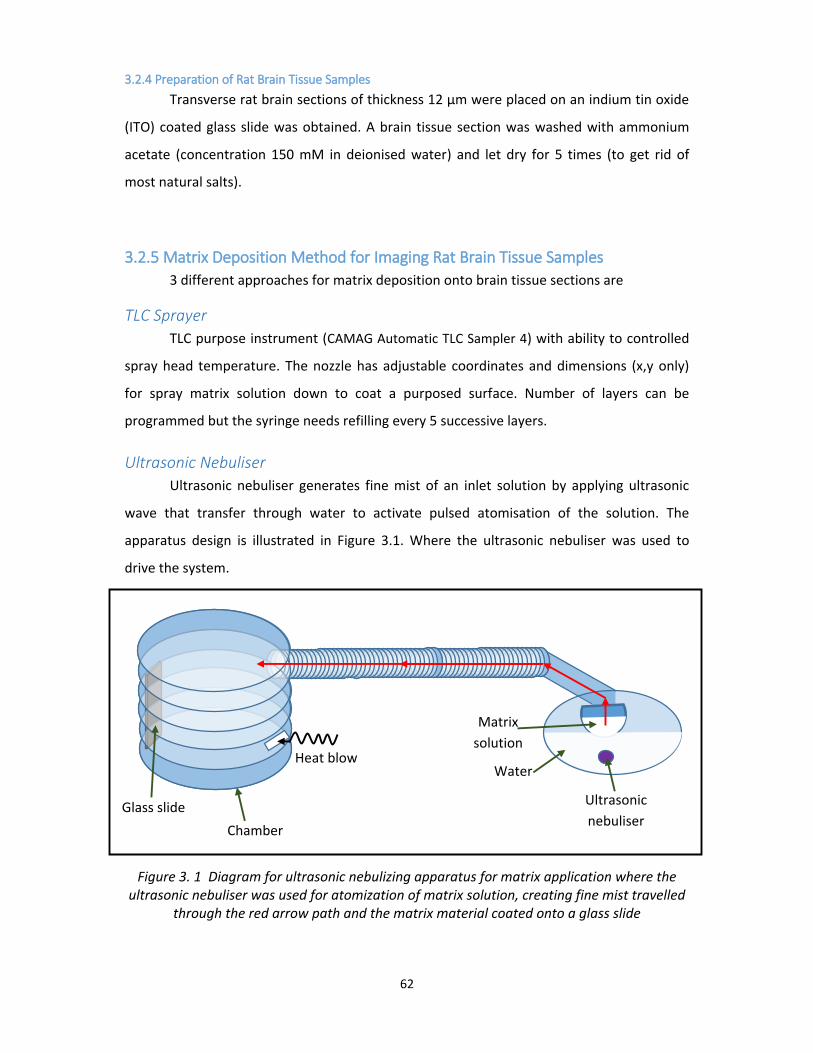
62
3.2.4 Preparation of Rat Brain Tissue Samples
Transverse rat brain sections of thickness 12 µm were placed on an indium tin oxide
(ITO) coated glass slide was obtained. A brain tissue section was washed with ammonium
acetate (concentration 150 mM in deionised water) and let dry for 5 times (to get rid of
most natural salts).
3.2.5 Matrix Deposition Method for Imaging Rat Brain Tissue Samples
3 different approaches for matrix deposition onto brain tissue sections are
TLC Sprayer
TLC purpose instrument (CAMAG Automatic TLC Sampler 4) with ability to controlled
spray head temperature. The nozzle has adjustable coordinates and dimensions (x,y only)
for spray matrix solution down to coat a purposed surface. Number of layers can be
programmed but the syringe needs refilling every 5 successive layers.
Ultrasonic Nebuliser
Ultrasonic nebuliser generates fine mist of an inlet solution by applying ultrasonic
wave that transfer through water to activate pulsed atomisation of the solution. The
apparatus design is illustrated in Figure 3.1. Where the ultrasonic nebuliser was used to
drive the system.
Figure 3. 1 Diagram for ultrasonic nebulizing apparatus for matrix application where the ultrasonic nebuliser was used for atomization of matrix solution, creating fine mist travelled
through the red arrow path and the matrix material coated onto a glass slide
Glass slide
Chamber
Heat blow
Ultrasonic
nebuliser
Water
Matrix
solution

63
SunCollect
The SunCollect (SunChrom, Germany) generate jet of spray using pneumatic
nebulising method. The nozzle has adjustable coordinates and dimensions (x,y,z) for spray
matrix solution down to coat a purposed surface. Number of layers can be programmed and
run continuously.
3.2.6 Calibration Standard
A standard for calibration of mass spectrometry measurement was made from mixed
solution of 3 peptides, including reserpine, angiotensin and ProteoMass™ P14R MALDI-MS
Standard (P14R), as recommended by manufacturer.
3.3 MALDI-MS Apparatus Settings and Acquisition Parameters The MALDI-TOF-MS instrument used at the Wolfson Molecular Imaging Centre
(WMIC), the University of Manchester is MALDI-MS instrument from Kratos (a Shimadzu
group company) which had been upgraded to be effectively equivalent to the “Axima
Performance MALDI- ToF2-MS” instrument as mentioned in Section 2.4.1. This was the main
instrument to perform experimental works in this report (without stating otherwise, this is
the one used). It has a 1 kHZ laser with beam diameter about 100 µm. The type of laser is
frequency-tripled Nd:YAG UV laser of wavelength 353 nm. In each experiment, Laser power
was adjusted such that the signal to noise is optimised, and would be kept constant
throughout the experimental session.
In lipid MS acquisition, mass range 1-1500 Da was selected and pulse extraction was
optimised at molecular mass of 750 Da. (mass range 1-2500 Da, and pulse extraction
optimised at 1250 Da for calibration) Collision induced dissociation (CID) is operated with
helium gas for acquisition in MS/MS mode. Ions with masses fall within the ion gate at a
selected mass peak, with a mass resolution down to 200.
The 7090 model of MALDI-TOF2-MS instrument available at the Kratos Analytical
Laboratory in Manchester were used to perform part of MS imaging experiment in Section
3.4.3. It has a 2 kHZ laser pulse of type (solid state UV laser, frequency tripled Nd:YAG),

64
wavelength 353 nm. It has tuneable laser beam diameter which was set to be 50 µm when
acquire data in the experiment.
3.4 Experiments
3.4.1 Initial Tests of Instrumental and Technical Performance
This experiment was carried out using the extract lipid from cow’s milk sample and
the recrystallised DHB matrix (see Section 3.2.1 and 3.2.2 for preparing instructions). In each
MS measurement, 200 profiles of MS spectra were acquired with 5 laser shots per profiles,
and recorded accumulatively. Where laser was moved randomly within the region of
interest.
First of all, the standard method of sample-matrix deposition which is “matrix top”
method as refer to Section 3.2.3 was used to test for an appropriate thickness of sample-
matrix depositions onto the metal surface, determined by varying number of application
layers. With a selected thickness, laser power was varied to observe signal-to-noise ratio
(S/N), signal intensity and mass resolution of a specific peak, 760.5 m/z, providing that the
scale for laser power in the instrument is in an arbitrary unit. For the laser power that gave
the most appropriate results, it was selected to be used throughout the repeatability tests in
the following experimental Section 3.4.2. This test was performed on each of the matrix-
sample application techniques, spotting (matrix top) and TLC spraying on a metal plate and
an ITO glass slide (see Section 3.2.3 for application methods)
Mass spectra were acquired from calibration spots at varied locations on the same
target plate to test for systematic errors in mass measurement due to laser fired at different
spatial locations. Blank matrix mass spectra were also obtained only for reference.
3.4.2 Mass Spectra from Milk Samples
Repeatability Tests of MS Spectra from Milk Samples
In this experiment, the extract lipid from cow’s milk sample and the recrystallised
DHB matrix were used. A MS measurement was acquired in the same way as in
experimental Section 3.4.1 (200 profiles of MS spectra, 5 laser shots per profiles). Sample-
matrix deposition method in every sample-matrix deposition methods mentioned in Section

65
3.2.3 are compared. The following 2 sets of MS measurements were considered for every
sample-matrix deposition methods.
1.) Between-well repeatability : A single MS measurement was acquired from each of
the 3 repeat depositions of same sample in separate wells. For every MS
measurement, laser was fired at random within a corresponding well.
2.) Within-well repeatability : 5 repeat MS measurements were acquired from the same
deposition of sample in a well. Laser was fired at random.
When the TLC sprayer approach was repeat to apply sample-matrix onto an ITO glass slide,
the repeatability tests were conducted onto relatively same defined well regions as in the
metal plate.
*Please see Section 3.5 for pre-processing of data and the result Section 4.2.1 for variance
analysis.
Measure of Milks’ Concentrations
Cow’s and goat’s milk samples were mixed at various concentrations before solvent
extraction at ratios 100:0, 75:25, 50:50, 25:75 and 0:100 (cow’s milk : goat’s milk, by
volume). A suitable sample-matrix application method to be used here was selected from
the previous section as will be discussed in the result Section 4.2.2. Peak area ratios from
each milk concentration were calculated to find out correlations with relative concentration.
Characterisation of Milk Spectra (MS/MS)
MS/MS spectra were acquired for 4 selected peaks, 734.5, 760.5, 782.5 and 786.5
m/z. The characteristics of these MS/MS spectra were observed when the ‘matrix top’
application method was used. Acquisition and laser parameters were kept the same as in
their MS mode apart from the added ion gates selected at mass resolution ≤200 for a
specific MS peak to undergo fragmentation via CID and obtain second stage MS
measurement (see Section 3.3 for other parameter settings)

66
3.4.3 Mass Spectrometry Imaging
Comparison of Matrix Coating Techniques
The appearance of matrix coated onto normal glass slides as a result of different
coating techniques: TLC sprayer, SunCollect, and ultrasonic nebuliser (see Section 3.2.5),
were observed under a microscope. Determination of amounts of matrix coated onto a glass
slide area were measured by high performance liquid chromatography (HPLC) part of a
Shimadzu instrument with an absorption detector (wavelength range 200-800 nm). The LC
column used was an ACE 3C18-HL, dimension 150×4.6 mm with a reversed phase method.
First, the calibration curve was generated from known concentrations of non-recrystallised
DHB (Sigma-Aldrich product) which varied between 0.05 mg/ml and 1.0 mg/ml. Matrix
deposited on glass slide was re-dissolved in acetonitrile:water (1:1). A known proportion of
this was taken for identification. Evaporation and re-dissolution again in known (smaller)
volume of the solvent was sometimes required in case low concentration of matrix was
being measured.
Mass Spectrometry Imaging of Rat Brain Tissues
Number of layers of successive matrix applications (using TLC sprayer and SunCollect
machine) and concentrations of DHB matrix were varied to try to optimise preparation
method. For an image acquisition, spatial resolution can be varied. One profile was acquired
at a spatial location where 50 laser shots per profile was used across acquisition region.
MS images from the sample acquisitions were viewed in Biomap software using the
identical m/z peaks, 734.5, 760.5, and 788.5 to create a map of intensity of the selected m/z
peak at every spatial pixel of the acquired sample area. The Biomap software was developed
by Rausch and Stoeckli (Novartis) (available from: http://www.maldi-msi.org/index.php?
option=com_content&view=article&id=14&Itemid=32).
3.5 Pre-processing Analysis of Mass Spectra For further spectral analysis, mass spectra were recorded as the accumulated signals
from all profiles recorded. With baseline correction, the mass spectra of all sample-matrix
deposition methods from Section 3.4.2, either the raw data or processed data using spline
interpolation, were compared to determine the variance of ratios between peak areas of 2

67
selected ion peaks (see the result in Section 4.2.1). Where the peak 760.5 vs 734.5 m/z were
selected from cow’s milk spectra because they were observed as major peaks in every
acquisition and also in MSI spectra of rat brain tissue. These peak appears in phospholipid
mass range as stated in Veloso et al. (2011) in a study of lipid distribution in human brain. A
simple approach for baseline correction was performed, where a baseline was estimated by
linear interpolation of minimum points in each of the 30 data point intervals, respectively,
throughout the full range of spectrum as demonstrated in Figure 3.2. Then, the original
spectrum was subtracted by the estimated baseline. This was coded in Matlab (see
Appendix). Note that the same approach for baseline correction was also used in the
experiment observing for change in some peak area ratios with the relative milk
concentration. Integrating over a full-width half maximum region of peak at a specific m/z in
a mass spectrum is an approach to determine a peak area to calculate peak area ratios in
both the repeatability and concentration tests. Figure 3.3 demonstrates the plots of 2
different peaks from multiple MS measurements. The Matlab codes for obtaining values for
peak area ratio are also shown in Appendix.
If spectral alignment was necessary, SpecAlign software (free software developed by
Dr Jason Wong, the University of Oxford, available from: http://ptcl.chem.ox.ac.uk/~jwong/
specalign) has options to align all mass spectra against their averaged mass spectrum (Wong
et al., 2005).

68
Figure 3. 2 Baseline correction for mass spectrum : Blue line indicates a mass spectrum where blue circles are raw data points in the spectrum, and red line indicates an estimated baseline with the red crosses being minimum points in each of the 30 data point intervals

69
Figure 3. 3 Plot of peak m/z 760.5 vs 734.5 with MS measurements from different cow’s-to-goat’s milk concentrations
4. Results and Disscussion
4.1 Initial Tests of Instrumental and Technical Performance
4.1.1 Thickness of Sample-matrix Materials
Figure 4.1 shows microscopic appearance of how sample-matrix crystals were
formed in wells using the “matrix top” method of application with 1, 2 and 3 layers applied.
a.) 1 layer b.) 2 layers c.) 3 layers
Figure 4. 1 Matrix top applications of cow’s milk samples with different numbers of sample-matrix application layers (all at the same magnification)
1mm

70
Higher energy was needed to generate a similar ion current when there were thicker
materials coated on the metal surface of the target plate. 1-layer application formed a thin
layer of material onto the metal surface, hence starting to obtain mass spectra at the lowest
threshold laser power. The mass spectra produced under these conditions were relatively
noisy, which may relate to the fact that not enough analyte was deposited in the well.
Figure 4.1(a) shows also that the crystal size for the 1-layer one was relatively large and
distributed unevenly. In comparison, Figure 4.1(b) indicating the 2-layer application shows a
more homogeneous distribution through the well with more analyte present. 3-layer
deposition not only increases the chances of spilling of material outside the well, but also
generates higher background noise level compared to the 2-layer method. This will be
discussed Section 4.1.4. Thus, the 2-layer application method was selected for use in further
experiments.
4.1.2 Laser Power
For the “matrix top” spotting technique on metal plates, with the TLC spraying
technique on metal plates and on ITO glass slides, MS measurements were acquired across
a range of laser powers from 90-180 (arbitrary units). Figures 4.2, 4.3 and 4.4 show S/N,
signal intensity (top) and mass resolution (bottom) as a function of laser power for MALDI
peak 760.5 m/z of milk sample from these 3 different deposition methods, respectively.
Note that all mass resolutions quoted here use the full-width half maximum (FWHM)
definition (see the definition for mass resolution in Section 2.2.6).
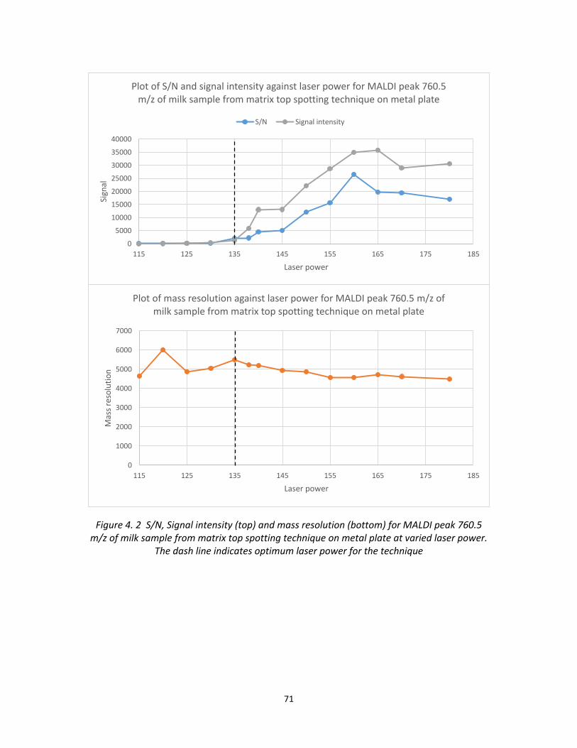
71
Figure 4. 2 S/N, Signal intensity (top) and mass resolution (bottom) for MALDI peak 760.5 m/z of milk sample from matrix top spotting technique on metal plate at varied laser power.
The dash line indicates optimum laser power for the technique
0
5000
10000
15000
20000
25000
30000
35000
40000
115 125 135 145 155 165 175 185
Sign
al
Laser power
Plot of S/N and signal intensity against laser power for MALDI peak 760.5 m/z of milk sample from matrix top spotting technique on metal plate
S/N Signal intensity
0
1000
2000
3000
4000
5000
6000
7000
115 125 135 145 155 165 175 185
Mas
s re
solu
tio
n
Laser power
Plot of mass resolution against laser power for MALDI peak 760.5 m/z of milk sample from matrix top spotting technique on metal plate

72
Figure 4. 3 S/N, Signal intensity (top) and mass resolution (bottom) for MALDI peak 760.5 m/z of milk sample from TLC spraying technique on metal plate at varied laser power. The
dash line indicates optimum laser power for the technique
0
5000
10000
15000
20000
25000
30000
35000
40000
115 125 135 145 155 165 175 185
Sign
al
Laser power
Plot of S/N and signal intensity against laser power for MALDI peak 760.5 m/z of milk sample from TLC spraying technique on metal plate
S/N (metal) Signal intensity (metal)
0
1000
2000
3000
4000
5000
6000
7000
115 125 135 145 155 165 175 185
Mas
s re
solu
tio
n
Laser power
Plot of mass resolution against laser power for MALDI peak 760.5 m/z of milk sample from TLC spraying technique on metal plate

73
Figure 4. 4 S/N, Signal intensity (top) and mass resolution (bottom) for MALDI peak 760.5 m/z of milk sample from TLC spraying technique on glass slide at varied laser power. The
dash line indicates optimum laser power for the technique
For all sample-matrix application methods, the measured signal intensity and S/N at
a specific peak (760.5) increased with increasing laser power with a plateau at higher laser
powers. In contrast, mass resolution decreased as a function of laser power. This usually
starts to be obvious approximately at the laser power where S/N >200. Below this point the
mass resolution was found randomly fluctuated, as shown in the bottom graphs of Figure
4.2, 4.3 and 4.4 usually at laser regions below the dash lines. Since, the detection limit of
0
5000
10000
15000
20000
25000
30000
35000
40000
115 125 135 145 155 165 175 185
Sign
al
Laser power
Plot of S/N and signal intensity against laser power for MALDI peak 760.5 m/z of milk sample from TLC spraying technique on ITO glass slide
S/N Signal intensity
0
1000
2000
3000
4000
5000
6000
7000
115 125 135 145 155 165 175 185
Mas
s re
solu
tio
n
Laser power
Plot of mass resolution against laser power for MALDI peak 760.5 m/z of milk sample from TLC spraying technique on ITO glass slide

74
saturation was another factor to be concerned. Then, an appropriate laser power was
selected such that the detection voltage would not exceed 100 mV and still generate good
results (S/N) for quantitation. The selected laser power of 135 for “matrix top” methods are
also used for all other spotting methods. Whereas those TLC spraying method on both
applying surface used 137 laser power.
4.1.3 Calibration
Calibration standard showed expected mass spectra as a result of MALDI-TOF-MS
measurement, allowing 500 mDa tolerance for peak adjustment, as seen in Figure 4.5. This
original calibration spectra was acquired at well position A1. Where Figure 4.6 is a diagram
of the slide showing the positions of the calibration standards deposited on the metal
target.
Figure 4. 5 Calibration spectra with peaks 609.7, 1046.5 and 1533.9 m/z
Variations in the measured m/z of mass peaks were observed to be a function of horizontal
spatial location at which the laser was fired on the metal target plate as summarised in
Figure 4.7 (left). Whereas no obvious trends observed from position in the vertical direction
as seen in Figure 4.7 (right).
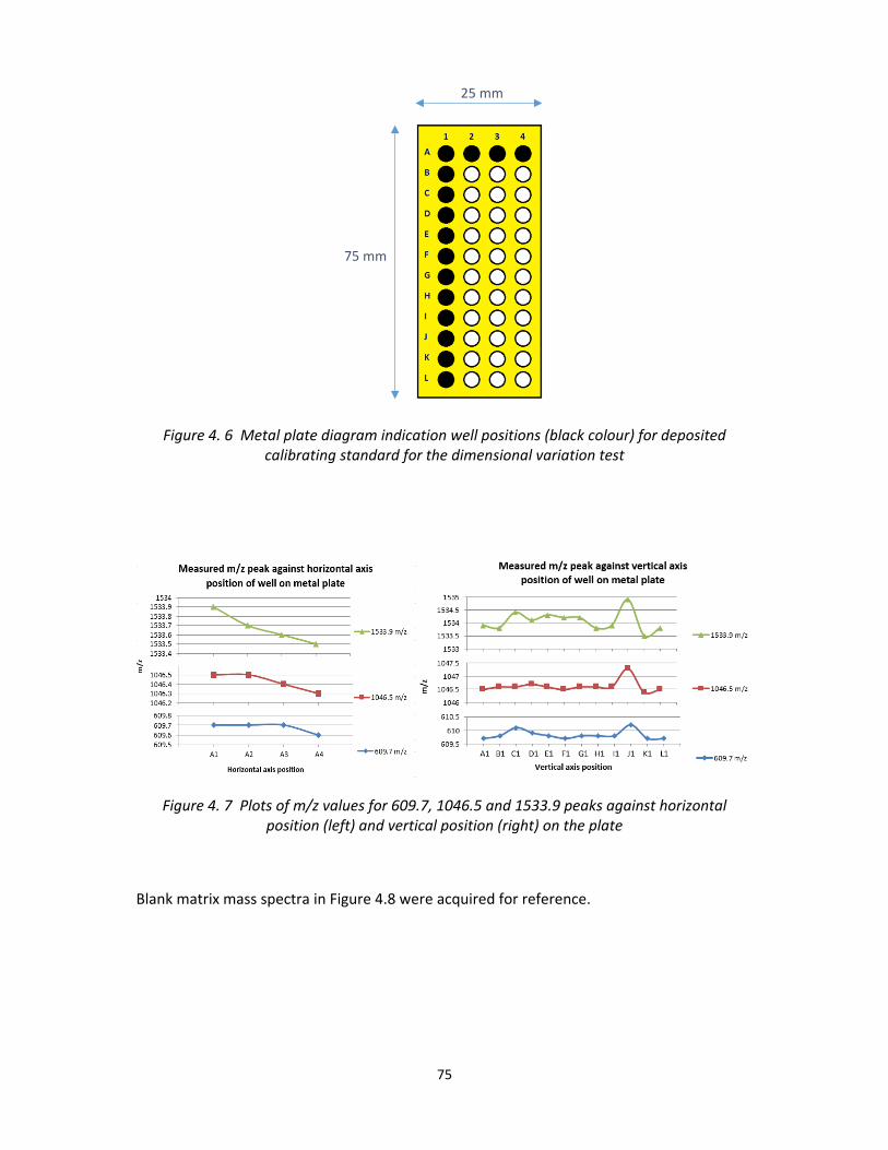
75
Figure 4. 6 Metal plate diagram indication well positions (black colour) for deposited calibrating standard for the dimensional variation test
Figure 4. 7 Plots of m/z values for 609.7, 1046.5 and 1533.9 peaks against horizontal position (left) and vertical position (right) on the plate
Blank matrix mass spectra in Figure 4.8 were acquired for reference.
25 mm
75 mm
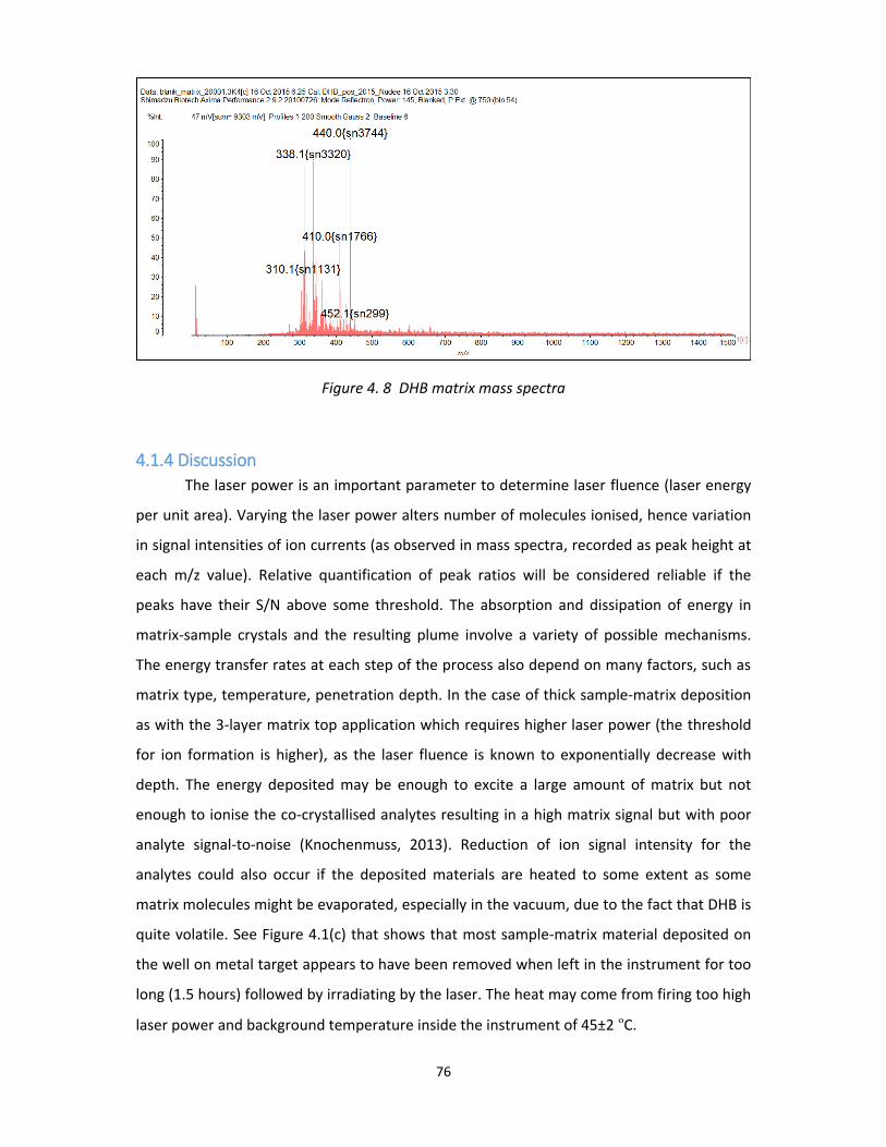
76
Figure 4. 8 DHB matrix mass spectra
4.1.4 Discussion
The laser power is an important parameter to determine laser fluence (laser energy
per unit area). Varying the laser power alters number of molecules ionised, hence variation
in signal intensities of ion currents (as observed in mass spectra, recorded as peak height at
each m/z value). Relative quantification of peak ratios will be considered reliable if the
peaks have their S/N above some threshold. The absorption and dissipation of energy in
matrix-sample crystals and the resulting plume involve a variety of possible mechanisms.
The energy transfer rates at each step of the process also depend on many factors, such as
matrix type, temperature, penetration depth. In the case of thick sample-matrix deposition
as with the 3-layer matrix top application which requires higher laser power (the threshold
for ion formation is higher), as the laser fluence is known to exponentially decrease with
depth. The energy deposited may be enough to excite a large amount of matrix but not
enough to ionise the co-crystallised analytes resulting in a high matrix signal but with poor
analyte signal-to-noise (Knochenmuss, 2013). Reduction of ion signal intensity for the
analytes could also occur if the deposited materials are heated to some extent as some
matrix molecules might be evaporated, especially in the vacuum, due to the fact that DHB is
quite volatile. See Figure 4.1(c) that shows that most sample-matrix material deposited on
the well on metal target appears to have been removed when left in the instrument for too
long (1.5 hours) followed by irradiating by the laser. The heat may come from firing too high
laser power and background temperature inside the instrument of 45±2 ºC.

77
We can assume that laser power was approximately in the order of 108 W/cm2 at the
threshold for signal detection of most organic molecules crystallised with DHB
(corresponding to an instrumental measure of laser power of about 135) as this is usually
the threshold for completion of desorption and ionisation processes (Morrical et al., 1998).
Figures 4.2, 4.3 and 4.4 (top graphs) shows that the signal intensity increases with the laser
power, then levels off possibly because of a saturation effect.
Most of the peaks from the calibration standard spectra at different plate locations
varied in mass within ±0.5 Da from the accepted m/z values as shown in Figure 4.7 which
was expected from the tolerance limit of the instrument. Rare cases with greater
uncertainty could come from other influences on mass accuracy. One could be
inhomogeneity of deposited surface thickness (see Figure 4.9) that was not taken into
account but can alter flight-time measurements of identical analytes. Another one could be
that measuring and detecting very low concentrations of standard at specific points might
give poor quality spectra, especially with the uneven spread of the isotopomer of the major
calibration peaks that may be more concentrated in some deposited region can lead to a
wrong peak being picked as an expected calibration peak.
Figure 4. 9 Calibration spot in metal target’s well
1mm
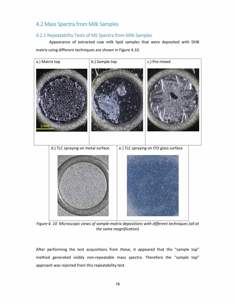
78
4.2 Mass Spectra from Milk Samples
4.2.1 Repeatability Tests of MS Spectra from Milk Samples
Appearance of extracted cow milk lipid samples that were deposited with DHB
matrix using different techniques are shown in Figure 4.10.
a.) Matrix top b.) Sample top c.) Pre-mixed
d.) TLC spraying on metal surface e.) TLC spraying on ITO glass surface
Figure 4. 10 Microscopic views of sample-matrix depositions with different techniques (all at the same magnification)
After performing the test acquisitions from these, it appeared that the “sample top”
method generated visibly non-repeatable mass spectra. Therefore the “sample top”
approach was rejected from this repeatability test.
1mm

79
All other deposition methods were included in a within-well and the between-well
repeatability assessment. From the recorded spectra, the ratio between 760.5 and 734.5
m/z peak areas (FWHM), calculated using Matlab code, are used for data analysis. These
were done by the analysis of variance (ANOVA) calculation. The results are summarised in
Table 4.1.
Table 4. 1 Summary of ANOVA for peak area ratios (760.5 vs 734.5 m/z) resulted from different sample-matrix deposition methods
Method
Raw data Interpolated data
Source of
variation
Degrees
of
freedom
Mean
square
deviation
F-
statistic
value
Source of
variation
Degrees
of
freedom
Mean
square
deviation
F-
statistic
value
Matrix top Between-well 2 0.0514 6.94 Between-well 2 0.0497 7.00
Within-well 12 0.0074 Within-well 12 0.0071
Total 14 0.0439 Total 14 0.0421
Pre-mixed Between-well 2 0.0066 0.54 Between-well 2 0.0064 0.53
Within-well 12 0.0122 Within-well 12 0.0120
Total 14 0.0443 Total 14 0.0436
TLC spraying
(metal
plate)
Between-well 2 0.0099 0.64 Between-well 2 0.0086 0.54
Within-well 12 0.0153 Within-well 12 0.0158
Total 14 0.0561 Total 14 0.0572
TLC spraying
(ITO glass
slide)
Between-well 2 0.0083 0.60 Between-well 2 0.0094 0.67
Within-well 12 0.0137 Within-well 12 0.0141
Total 14 0.0499 Total 14 0.0517
The F-statistic values were determined by dividing between-well and within-well
variances. To test the null hypothesis that all wells are identical, the critical value for F with
variances’ degrees of freedom of 2 and 12 in the first and second sources of variation is
given 3.885 (P=0.05) (Miller and Miller, 2010). Only the “matrix top” method exceeds this
value and leads to rejection of the null hypothesis. Whereas all other method gave much

80
lower F-value than the critical value which represents low variations of MS measurements
between wells compared to inside the wells.
4.2.2 Measure of Milks’ Concentrations
TLC spraying deposition method on metal and glass surface which has been proved
in the previous section as one of the between-well repeatable methods, were selected for
using in this experiment as interesting because the method will also be used to perform
matrix application onto tissue samples. Best Linear fits of peak area ratios (760.5 vs 706.5
m/z) against the cow’s milk concentration in cow’s and goat’s milk mixtures are as follows,
with the plots illustrated in Figure 4.11.
For using TLC spraying method on the metal plate,
𝑦 = (−0.036 ± 0.004)x + (5.439 ± 0.267)
For using TLC spraying method on the ITO glass slide,
𝑦 = (−0.042 ± 0.006)𝑥 + (6.069 ± 0.373)
Figure 4. 11 Plot of peak area ratio between 760.5 and 706.5 m/z peaks against cow’s milk concentration (% by volume) using TLC spraying method of deposition on metal plate (blue)
and glass slide (red) where error bars were determined by standard deviations from the mean of peak area ratios at each concentration from 4 repeated MS measurements from
same sample deposited in 4 different wells-i.e. 1 measurement per well
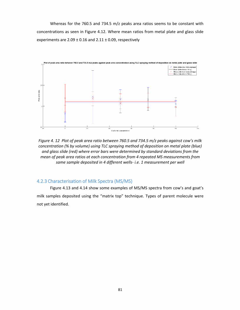
81
Whereas for the 760.5 and 734.5 m/z peaks area ratios seems to be constant with
concentrations as seen in Figure 4.12. Where mean ratios from metal plate and glass slide
experiments are 2.09 ± 0.16 and 2.11 ± 0.09, respectively
Figure 4. 12 Plot of peak area ratio between 760.5 and 734.5 m/z peaks against cow’s milk concentration (% by volume) using TLC spraying method of deposition on metal plate (blue)
and glass slide (red) where error bars were determined by standard deviations from the mean of peak area ratios at each concentration from 4 repeated MS measurements from
same sample deposited in 4 different wells- i.e. 1 measurement per well
4.2.3 Characterisation of Milk Spectra (MS/MS)
Figure 4.13 and 4.14 show some examples of MS/MS spectra from cow’s and goat’s
milk samples deposited using the “matrix top” technique. Types of parent molecule were
not yet identified.

82
a
b
c
d
Figure 4. 13 MS/MS spectra of cow’s milk for a.) 734.5, b.) 760.5, c.) 782.5 and d.) 786.5 m/z

83
a
b
c
d
Figure 4. 14 MS/MS spectra of goat’s milk for a.) 734.5, b.) 760.5, c.) 782.5 and d.) 786.5 m/z
84
4.2.4 Discussion
It can be suggested that the “matrix top” approach produces quite a uniform spread
of sample with a large excess of solvent evaporated (chloroform and methanol) before the
application of matrix, making the sample and matrix mix and interact reasonably well in the
first sample-matrix application layer. Then, the second layer of sample-matrix application
may re-dissolve part of the first layer deposition, and hence re-crystallisation more
uniformly with slower interaction processes. Different sample-matrix deposition methods
led to significantly different surface appearance as seen in Figure 4.10. The best data
appear to come from well mixed (co-crystallised) sample and matrix. The solvent allows this
mixing to happen but only once both sample and matrix are on the slide. Mixing was very
poor for “sample top” approach (i.e. matrix-analyte crystals were formed only in some
places in the well and the acquired mass spectra were not so repeatable), better for the
widely used “matrix top”, but significantly better for the other approaches (including pre-
mixed spotting and spraying methods). From analysis of variance of mass spectra acquisition
for the specific peak ratios 760.5 vs 734.5 m/z, the raw data acquired form sample
deposited by the pre-mixed spotting methods and the spraying method on metal and glass
surfaces have their F-values equal to 5.4, 6.4 and 6.0, respectively, which conclude that the
MS measurements were not differ from deposition to deposition of same method (P=0.05).
Also, the spline interpolation method did not make significant changes in the F-values,
hence, only the raw data were used for analysing the milk concentration experiment in this
report.
The methods of greatest interest were the TLC spraying deposition method on metal
and glass surface since the TLC spray was also used to perform matrix application task onto
tissue samples. Furthermore, it was successfully used to compare the results from 2
different types of targets (metal plate and glass slide) with exactly the same conditions, i.e.
same sample-matrix deposition method, same sample and matrix solution were used. This
provided very good results in obtaining linear correlation of the peak area ratios (760.5 vs
706.5 m/z) as described in Section 4.2.2. Thus, the analysis method can be improved with a
more advanced algorithms using more spectral information towards relative or even
absolute quantitation tasks. Together with tandem mass spectrometry (MS/MS), substances
that give rise to the important spectral peaks can be identified. Similarly, this approach will
be assessed in the quantitative mass spectrometry imaging.

85
4.3 Mass Spectrometry Imaging
4.3.1 Comparison of Matrix Coating Techniques
Matrix Surface Appearance on Glass Slide
The 3 different coating techniques: TLC Sprayer, SunCollect, ultrasonic nebuliser
systems, showed different DHB crystal appearance on glass slide surface under microscope
as illustrated in Figure 4.15.
a.) TLC sprayer b.) SunCollect c.) Ultrasonic Nebuliser
Figure 4. 15 Microscopic views with same magnification of matrix coated onto glass slide via (a.) TLC Sprayer, (b) SunCollect and (c) Ultrasonic nebuliser systems
Quantity of Matrix Coated onto Glass Slide Figure 4.16 shows a calibration curve for the DHB matrix concentrations from HPLC
measurements. The Sigma-Aldrich DHB product was used. The quantity of matrix that was
deposited onto each of the glass slide using the different methods can then be determined
by washing off the slide followed by HPLC analysis. The results are given in Table 4.2 where
the expected values was determined from the instrumental parameter settings, measured
values are calculated from the HPLC analysis results, and the uncertainties were determined
by the difference of the measured value from its corresponding expected value.
100 µm

86
Figure 4. 16 Calibration curve for measuring DHB concentrations : A plot of area under DHB peak at detected spectroscopy wavelength 254 nm against DHB concentration
The following parameters were set for measurements.
TLC Sprayer standard : 10 mg/ml, 2 µl per layer, application area 15x15 mm
SunCollect : Flow rate 20ml/min, medium nozzle speed, application area 25x75 mm
Ultrasonic nebuliser : 10 mg/ml, 100 ml total volume used, application area 25x75 mm
Table 4. 2 Estimated DHB matrix quantity deposited on glass slide using different application methods
Matrix application
method
Number of DHB molecules per mm2 per layer
(×1014) Uncertainty (%)
Expected value Measured value
TLC sprayer 3.47 3.58 3.17
SunCollect 5.43 4.09 24.7
Ultrasonic nebuliser - 4.88 -
y = 3E+06x + 73650 R² = 0.9998
0
500000
1000000
1500000
2000000
2500000
3000000
3500000
4000000
0 0.2 0.4 0.6 0.8 1 1.2
Pea
k ar
ea
DHB concentration
Plot of peak area for absorbtion wavelength 254 nm against DHB concentration
254 nm
Linear (254 nm)

87
4.3.2 Mass Spectrometry Imaging of Rat Brain Tissues
This section introduces some successfully acquired mass spectrometry images as a
result of current approach of sample preparation procedures, and MSI instruments and
acquisition parameters.
The Image of a rat brain tissue section in Figure 4.17 showed the distribution plot of
mass peak m/z 760.5. The image used the TLC spraying techniques to apply DHB matrix
(recrystallised product from LASER Biolabs) onto the brain tissue samples. It was applied
with 2µl × 15 layers of 10 mg/ml and 20 mg/ml DHB concentrations on either half
(application area 15 × 15 mm) and were acquired using the AXIMA instrument. It has spatial
resolution about 100 µm.
Figure 4. 17 Mass spectrometry image (at m/z 760.5) of a brain tissue section with varied DHB matrix (recrystallised) concentration, 10 mg/ml (left half) and 20 mg/ml (right half)
applied using the TLC sprayer, acquired using the AXIMA instrument. The image was obtained using Biomap software with the colour scale indicating normalised signal intensity.
It should be that the amount of matrix applied when 10 mg/ml of DHB concentration were
used was enough to see some anatomical brain structure as seen in the left half of the MSI
in Figure 4.17.
Higher spatial resolution images were acquired with the 7090 model of MALDI
instrument with use of the SunCollect for matrixes application. Total number of matrix
application layers were 20 layers. The matrix application flow rates for the first and second
%int
100
0

88
layers of matrix application were 10 and 15 ml/min, respectively, as spray base layer to
retain localisation of analytes in a brain tissue section (not to over-wet the tissue). Then a
constant flow rate of 20 ml/min was used for all remaining 18 layers. Rate at which the
spray head move was set to medium. 2 types of DHB matrix of same concentration (10
mg/ml) were applied onto 2 brain tissue sections and the MS images in Figure 4.18 obtained
using the recrystallised (Laser Biolabs) and non-recrystallised DHB (Sigma-Aldrich) products
were acquired with spatial resolutions of 70 µm and 100 µm, respectively.
%int Recrystallised DHB Non-recrystallised DHB
100
788.9 m/z 788.9 m/z
0 734.5 m/z 734.5 m/z
Figure 4. 18 Mass spectrometry images (788.9 vs 734.5 m/z) of brain tissue sections with DHB matrix (recrystallised and non-recrystallised) concentration of 10 mg/ml SunCollect
sprayer, acquired using the 7090 instrument. The image was obtained using Biomap software with the colour scale indicating normalised signal intensity.
Figure 4.18 shows distinct MS characteristics in the region of their corpus callosum, septal
nuclei and anterior commissure. Where 788.9 m/z appears to be more concentrated than
the 734.5 m/z in these regions. This was observed in both MSIs acquired from the 7090
instrument.

89
4.3.3 Discussion
The TLC sprayer is currently a primary method of matrix applcation available at the
WMIC. Its intended purpose is for spraying TLC samples onto TLC plates, unlike the
SunCollect instrument which has built specifically for MALDI matrix application. The
SunCollect apparatus has been shown to create small matrix crystal size of diameter less
than 50 µm and lead to very homogeneous matrix deposited onto tissue surface (Römpp
and Spengler, 2013). To make the TLC sprayer perform similarly to SunCollect system was
managed (see Table 4.2 in Section 4.3.1 in terms of the number of molecules applied per
unit area per layer). This was also achieved with the ultrasonic nebuliser approach, apart
from the problem that this technique consumed about 1,000 times the amount of matrix
material and is not therefore economically useful. The interesting finding about this is that
this technique can, in theory, be optimised to achieve few µm of droplet size. It was also
shown in Figure 4.15(c) that the ultrasonic nebuliser generated an obviously different matrix
distribution from the other 2 spraying methods.
In imaging experiments, results are based on adjusting matrix deposition methods to
optimise the quality of mass spectrometry images. The apparent spatial resolution is not
only limited to the space between acquisition points (pixel size) and/or laser beam size the
but also the delocalisation of analytes in the tissue during sample preparation and matrix
application. For example, too wet a matrix solution application can make most of the lipid to
spread beyond the tissue. This can be prevented by having spray base-i.e. spray sheer layers
of matrix solution onto bare tissue section, then followed by larger volume of the matrix
solution in next applying layers as done to produce MSIs in Figure 4.18. The SunCollect has
the ability for the nozzle distance from the tissue surface to be adjusted. The matrix solution
would distribute more evenly with height and the pressure of application would be altered.
The AXIMA instrument have very long acquisition times, as it is limited by the data
transfer rates to a sampling rate of about 100 Hz. Anatomical information of the transverse
rat brain section were obtained at higher spatial resolution with the 7090 instrument
compared to the AXIMA. Also, mass spectra from the 7090 had much better mass accuracy
and the mass resolution (up to 10,000 FHWM), due to the longer flight path and
improvement in pulse extraction design. This is immediately clear in Figure 4.18 the brain
section images, showing the signal intensity difference between peaks (788.5 vs 734.5 m/z)

90
in corpus callosum, septal nuclei and anterior commissure regions of the brain. Further
analysis of the mass spectra in the regions of interest of the MS image will be needed to
express these signals quantitatively. Careful pre-processing data analysis such as spectra
alignment should improve the image quality to make better apparent resolution and
eliminate blurring.
5. Conclusions The capabilities of the Kratos Axima Performance MALDI- ToF2-MS instrument was
studied by observing the characteristics of mass spectra generated. Laser powers that led to
optimised signal-to-noise ratios were determined, given ion detection signals of ≤100 mV, to
achieve reasonable quantitative data analysis. The instrument was calibrated to an accuracy
of ±0.5 Da. Repeatability tests for each deposition method for the cow’s milk lipid extract
samples with DHB matrix were compared by variance analysis. The methods where sample
and matrix solutions were pre-mixed showed similar repeatability regardless the application
techniques-i.e. spotting or TLC spraying and were much more repeatable than the separate
spotting of matrix on top of the sample which is the widely used “dried droplet” approach. A
linear relationship between the ratio of integrated areas of two selected peaks and the
concentration of mixture of the two milk types was observed for mass spectral data
acquired on both metal and ITO glass surface using TLC spraying technique.
In imaging experiments, the SunCollect matrix applicator and the 7090 model of
MALDI-MS were found to be the best combination to generate good quality mass
spectrometry images in term of spatial resolution. Measurement of specific peak areas leads
to some distinctions between some regions of interest (parts of rat brain tissue) but it is not
yet clear to what extent these measurements are quantitative.
91
6. Summary of Future Work The project will focus on quantitative analysis of mass spectrometry imaging (MSI)
data. Independent component analysis (ICA) will be an approach to be used where the
dimensionality of the spectral data can be reduced to optimally represent entire spectrum
with minimal number of independent component spectra. ICA algorithms assume Poisson
statistics in determination of variances as should be expected in MS signal noise. In-house
software will be used to analyse mass spectrometry imaging data using an ICA algorithm. By
training the whole set of mass spectral data in the acquired MSI, an ICA model will be
generated. Where a mass spectrum is composed of component spectra, each with a
coefficient related to its quantity-i.e. the linear fraction of each component. The coefficient
value for each component spectrum will vary across pixels of the MSI acquisition, hence a
component image can be constructed from the plot of this quantity. Combination of
component spectra that globally best describe a particular MSI dataset would form an ICA
model specifically for that dataset.
In real biological tissue applications, MSI data should contain mass spectra that
characterise biological molecules contained within the tissue sample. Taking into account
useful component images which hold more or less the information from original spectra via
some multi-spectral analysis, mass spectra at each spatial location can then be classified
based on their tissue types. This should give more meaningful results describing distribution
of each tissue type, in contrast to the current approach to generate an MS image using the
specific m/z peak area which refers to a specific molecule.
Experimental work to this point has used an internal standard approach, measuring
the relative concentrations determined from the ratio of integrated peak areas has
demonstrated an ability to quantify. This approach could, with an appropriate internal
standard (perhaps delivered with the matrix) also be applicable to brain tissue samples.
Whereas the ICA approach will target tissue types which should return results of different
distributions of particular tissue in normal and diseased tissues. The two approaches could
be compared by looking at their signal-to-noise values across the images. Furthermore,
using an ICA model with a Monte-Carlo system should confirm that the real data have the
anticipated noise characteristics.

92
Collecting more useful MSI data from brain tissue sections will be an ongoing process
in the short term. Mainly, the 7090 MALDI-MS will be used with SunCollect matrix
application method as this is known to produce good quality images. MS Images taken from
the AXIMA instrument with other matrix application methods will also be improved and
compared. Also, an ICA model will be trained for some other sources of tissue, for example,
brain tissue with known brain disease and tissue with added internal standards. Tandem
mass spectrometry will also be an important tool to identify type of molecules of interest
and therefore describe tissue compositions. Please see Table 6.1 for a future work plan to
be undertaken in the second year of the PhD programme.
Table 6. 1 A second year plan of the research project
Month
Plan
1 2 3 4 5 6 7 8 9 10 11 12
Learn the in-house software for
ICA analysis and learn the basic of
how to programme in C language
(be able to load MS data and use
it in specific software)
Generate more MSI data from rat
brain tissue samples using the
7090 MALDI-MS instrument
Find suitable parameters and pre-
paration technique to optimise
the AXIMA MALDI-MS perfor-
mance on acquiring MSI data /
Find out about the order of
magnitude of instrumental di-
mension that affect variation in
calibration at varied location in
space
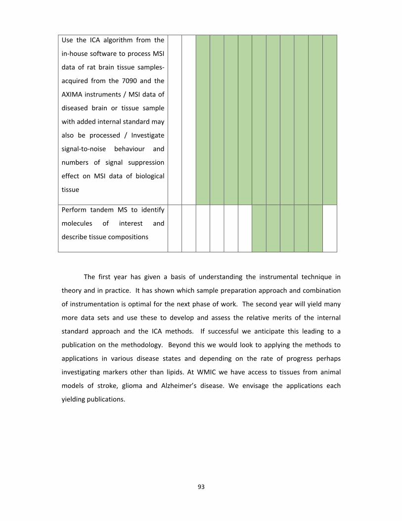
93
Use the ICA algorithm from the
in-house software to process MSI
data of rat brain tissue samples-
acquired from the 7090 and the
AXIMA instruments / MSI data of
diseased brain or tissue sample
with added internal standard may
also be processed / Investigate
signal-to-noise behaviour and
numbers of signal suppression
effect on MSI data of biological
tissue
Perform tandem MS to identify
molecules of interest and
describe tissue compositions
The first year has given a basis of understanding the instrumental technique in
theory and in practice. It has shown which sample preparation approach and combination
of instrumentation is optimal for the next phase of work. The second year will yield many
more data sets and use these to develop and assess the relative merits of the internal
standard approach and the ICA methods. If successful we anticipate this leading to a
publication on the methodology. Beyond this we would look to applying the methods to
applications in various disease states and depending on the rate of progress perhaps
investigating markers other than lipids. At WMIC we have access to tissues from animal
models of stroke, glioma and Alzheimer’s disease. We envisage the applications each
yielding publications.

94
References Adibhatla, Rao Muralikrishna, J. F. Hatcher, and R. J. Dempsey. "Lipids and Lipidomics in
Brain Injury and Diseases." The AAPS Journal 8, no. 2 (2006): E314-E21. Al-Saad, Khalid A., Vladimir Zabrouskov, William F. Siems, N. Richard Knowles, Richard M.
Hannan, and Herbert H. Hill. "Matrix-Assisted Laser Desorption/Ionization Time-of-Flight Mass Spectrometry of Lipids: Ionization and Prompt Fragmentation Patterns." Rapid Communications in Mass Spectrometry 17, no. 1 (2003): 87-96.
AlMasoud, N., Y. Xu, N. Nicolaou, and R. Goodacre. "Optimization of Matrix Assisted Desorption/Ionization Time of Flight Mass Spectrometry (Maldi-Tof-Ms) for the Characterization of Bacillus and Brevibacillus Species." [In English]. Analytica Chimica Acta 840 (Aug 20 2014): 49-57.
Bae, Y. J., J. C. Choe, J. H. Moon, and M. S. Kim. "Why Do the Abundances of Ions Generated by Maldi Look Thermally Determined?" [In English]. Journal of the American Society for Mass Spectrometry 24, no. 11 (Nov 2013): 1807-15.
Barber, M., R. S. Bordoli, R. D. Sedgwick, and A. N. Tyler. "Fast Atom Bombardment of Solids as an Ion Source in Mass Spectrometry." Nature 293, no. 5830 (09/24/print 1981): 270-75.
Bayer, S. A., J. Altman, R. J. Russo, and X. Zhang. "Timetables of Neurogenesis in the Human Brain Based on Experimentally Determined Patterns in the Rat." [In eng]. Neurotoxicology 14, no. 1 (Spring 1993): 83-144.
Bennett, Edward L., Marian C. Diamond, David Krech, and Mark R. Rosenzweig. "Chemical and Anatomical Plasticity of Brain." Science 146, no. 3644 (1964): 610-19.
Benningh.A. "Analysis of Submonolayers on Silver by Negative Secondary Ion Emission." [In English]. Physica Status Solidi 34, no. 2 (1969): K169-&.
Berg, J.M., J.L. Tymoczko, and L. Stryer. "Fatty Acids Are Key Constituents of Lipids." Chap. 12.2 In Biochemistry. New York: W. H. Freeman and Company, 2002.
Beynon, J. H., R. G. Cooks, J. W. Amy, Baitinge.We, and T. Y. Ridley. "Design and Performance of a Mass Analyzed Ion Kinetic-Energy (Mike) Spectrometer." [In English]. Analytical Chemistry 45, no. 12 (1973): 1023-&.
"Bioinformatics Toolbox." The MathWorks, Inc., http://uk.mathworks.com/products/bioinfo/.
"Biomap." Novartis, http://www.maldi-msi.org/index.php?option=com_content&view=article&id=14&Itemid=32.
Bligh, E. G., and W. J. Dyer. "A Rapid Method of Total Lipid Extraction and Purification." Can J Biochem Physiol 37, no. 8 (Aug 1959): 911-7.
Blumel, R. "The Dynamic Kingdon Trap - a Novel Design for the Storage and Crystallization of Laser-Cooled Ions." [In English]. Applied Physics B-Lasers and Optics 60, no. 2-3 (Feb-Mar 1995): 119-22.
Bordas-Nagy, Jozsef, Dominique Despeyroux, Keith R. Jennings, and Simon J. Gaskell. "Experimental Aspects of the Collision-Induced Decomposition of Ions in a Four-Sector Tandem Mass Spectrometer." Organic Mass Spectrometry 27, no. 4 (1992): 406-15.
Busch, K. L. "Desorption Ionization Mass-Spectrometry." [In English]. Journal of Mass Spectrometry 30, no. 2 (Feb 1995): 233-40.
Cameron, A. E., and D. F. Eggers. "An Ion Velocitron." [In English]. Review of Scientific Instruments 19, no. 9 (1948): 605-07.

95
Chapman, J. R. Practical Organic Mass Spectrometry: A Guide for Chemical and Biochemical Analysis. Wiley, 1995.
Cornish, T. J., and R. J. Cotter. "A Curved-Field Reflectron for Improved Energy Focusing of Product Ions in Time-of-Flight Mass Spectrometry." Rapid Commun Mass Spectrom 7, no. 11 (Nov 1993): 1037-40.
Criminisi, A., and J. Shotton. "Introduction: The Abstract Forest Model." Chap. 3 In Decision Forests for Computer Vision and Medical Image Analysis, edited by A. Criminisi and J. Shotton. Advances in Computer Vision and Pattern Recognition, 7-23: Springer London, 2013.
Dagan, S., and A. Amirav. "Electron-Impact Mass-Spectrometry of Alkanes in Supersonic Molecular-Beams." [In English]. Journal of the American Society for Mass Spectrometry 6, no. 2 (Feb 1995): 120-31.
Dahl, David A. "Simion for the Personal Computer in Reflection." International Journal of Mass Spectrometry 200, no. 1–3 (12/25/ 2000): 3-25.
Damnjanovic, B., B. Petrovic, J. Dimitric-Markovic, and M. Petkovic. "Comparison of Maldi-Tof Mass Spectra of [Pdcl(Dien)]Cl and [Ru(En)(2)Cl-2]Cl Acquired with Different Matrices." [In English]. Journal of the Serbian Chemical Society 76, no. 12 (2011): 1687-701.
Dashtiev, M., E. Wafler, U. Rohling, M. Gorshkov, F. Hillenkamp, and R. Zenobi. "Positive and Negative Analyte Ion Yield in Matrix-Assisted Laser Desorption/Ionization." [In English]. International Journal of Mass Spectrometry 268, no. 2-3 (Dec 1 2007): 122-30.
Davis, Gwilym G. . Applied Anatomy: The Construction of the Human Body. 2nd ed. Philadelphia&London: J. B. Lippincott Company, 1913.
Deininger, S., K. Meyer, and A. Walch. "Concise Interpretation of Maldi Imaging Data by Probabilistic Latent Semantic Analysis (Plsa)." (2012).
Dempster, A. J. "A New Method of Positive Ray Analysis." Physical Review 11, no. 4 (04/01/ 1918): 316-25.
Dolnikowski, G. G., M. J. Kristo, C. G. Enke, and J. T. Watson. "Ion-Trapping Technique for Ion Molecule Reaction Studies in the Center Quadrupole of a Triple Quadrupole Mass-Spectrometer." [In English]. International Journal of Mass Spectrometry and Ion Processes 82, no. 1-2 (Jan 20 1988): 1-15.
Duncan, M. W., H. Roder, and S. W. Hunsucker. "Quantitative Matrix-Assisted Laser Desorption/Ionization Mass Spectrometry." Brief Funct Genomic Proteomic 7, no. 5 (Sep 2008): 355-70.
Duncan, Mark W., Gabrijela Matanovic, and Anne Cerpa-Poljak. "Quantitative Analysis of Low Molecular Weight Compounds of Biological Interest by Matrix-Assisted Laser Desorption Ionization." Rapid Communications in Mass Spectrometry 7, no. 12 (1993): 1090-94.
Emerson, Beth, Jennifer Gidden, Jackson O. Lay, and Bill Durham. "A Rapid Separation Technique for Overcoming Suppression of Triacylglycerols by Phosphatidylcholine Using Maldi-Tof Ms." Journal of Lipid Research 51, no. 8 (2010): 2428-34.
Fahy, Eoin, Shankar Subramaniam, H. Alex Brown, Christopher K. Glass, Alfred H. Merrill, Robert C. Murphy, Christian R. H. Raetz, et al. "A Comprehensive Classification System for Lipids." European Journal of Lipid Science and Technology 107, no. 5 (2005): 337-64.
Fahy, Eoin, Shankar Subramaniam, Robert C. Murphy, Masahiro Nishijima, Christian R. H. Raetz, Takao Shimizu, Friedrich Spener, et al. "Update of the Lipid Maps

96
Comprehensive Classification System for Lipids." Journal of Lipid Research 50, no. Suppl (2009): S9-S14.
Field, F. H., and M. S. B. Munson. "Reactions of Gaseous Ions .14. Mass Spectrometric Studies of Methane at Pressures to 2 Torr." [In English]. Journal of the American Chemical Society 87, no. 15 (1965): 3289-&.
Fjeldsted, J. "Time-of-Flight Mass Spectrometry: Technical Overview." Agilent Technologies (2003).
Fuchs, Beate, Ariane Nimptsch, Rosmarie Süß, and Jürgen Schiller. "Capabilities and Drawbacks of Phospholipid Analysis by Maldi-Tof Mass Spectrometry." Chap. 6 In Lipidomics, edited by Donald Armstrong. Methods in Molecular Biology, 103-25: Humana Press, 2009.
Girod, Marion, Yunzhou Shi, Ji-Xin Cheng, and R. Graham Cooks. "Desorption Electrospray Ionization Imaging Mass Spectrometry of Lipids in Rat Spinal Cord." Journal of the American Society for Mass Spectrometry 21, no. 7 (7// 2010): 1177-89.
Glish, G. L., and D. J. Burinsky. "Hybrid Mass Spectrometers for Tandem Mass Spectrometry." [In English]. Journal of the American Society for Mass Spectrometry 19, no. 2 (Feb 2008): 161-72.
Griffith, K. S., and G. I. Gellene. "Experimental and Theoretical Evidence for a New Metastable Valence State of O2." [In English]. Journal of Physical Chemistry 97, no. 39 (Sep 30 1993): 9882-89.
Gross, J. H. Mass Spectrometry: A Textbook. Springer, 2004. Gross, J. H., and P. Roepstorff. Mass Spectrometry: A Textbook. Springer, 2011. Guilhaus, M. "Principles and Instrumentation in Time-of-Flight Mass-Spectrometry - Physical
and Instrumental Concepts." [In English]. Journal of Mass Spectrometry 30, no. 11 (Nov 1995): 1519-32.
Han, Xianlin, and Richard W. Gross. "Shotgun Lipidomics: Electrospray Ionization Mass Spectrometric Analysis and Quantitation of Cellular Lipidomes Directly from Crude Extracts of Biological Samples." Mass Spectrometry Reviews 24, no. 3 (2005): 367-412.
Hanahan, Douglas, and Robert A. Weinberg. "The Hallmarks of Cancer." Cell 100, no. 1 (2000): 57-70.
Hanahan, Douglas, and Robert A Weinberg. "Hallmarks of Cancer: The Next Generation." Cell 144, no. 5 (2011): 646-74.
Hanselmann, Michael, Ullrich Köthe, Marc Kirchner, Bernhard Y. Renard, Erika R. Amstalden, Kristine Glunde, Ron M. A. Heeren, and Fred A. Hamprecht. "Toward Digital Staining Using Imaging Mass Spectrometry and Random Forests." Journal of Proteome Research 8, no. 7 (2009/07/06 2009): 3558-67.
Harkewicz, Richard, and Edward A. Dennis. "Applications of Mass Spectrometry to Lipids and Membranes." Annual review of biochemistry 80 (2011): 301-25.
Harrison, A. G. Chemical Ionization Mass Spectrometry, Second Edition. Taylor & Francis, 1992.
Harrison, AlexG. "Chemical Ionization Mass Spectrometry of Hydrocarbons and Halohydrocarbons." Chap. 20 In Hydrocarbons and Halogenated Hydrocarbons in the Aquatic Environment, edited by B. K. Afghan, D. Mackay, H. E. Braun, A. S. Y. Chau, J. Lawrence, D. R. S. Lean, O. Meresz, et al. Environmental Science Research, 265-83: Springer US, 1980.
Harwood, J. L., and C. M. Scrimgeour. "Fatty Acid and Lipid Structure." In The Lipid Handbook with Cd-Rom, Third Edition, 1-36: CRC Press, 2007.

97
Hazama, Hisanao, Hirofumi Nagao, Ren Suzuki, Michisato Toyoda, Katsuyoshi Masuda, Yasuhide Naito, and Kunio Awazu. "Comparison of Mass Spectra of Peptides in Different Matrices Using Matrix-Assisted Laser Desorption/Ionization and a Multi-Turn Time-of-Flight Mass Spectrometer, Multum-Img." Rapid Communications in Mass Spectrometry 22, no. 10 (2008): 1461-66.
Herbert, C.G., and R.A.W. Johnstone. Mass Spectrometry Basics. CRC Press, 2002. Hillenkamp, Franz, Thorsten W. Jaskolla, and Michael Karas. "The Maldi Process and
Method." In Maldi Ms, 1-40: Wiley-VCH Verlag GmbH & Co. KGaA, 2013. Hu, Q., R. J. Noll, H. Li, A. Makarov, M. Hardman, and R. Graham Cooks. "The Orbitrap: A
New Mass Spectrometer." J Mass Spectrom 40, no. 4 (Apr 2005): 430-43. Hulbert, A. J., and Paul Lewis Else. "Membranes as Possible Pacemakers of Metabolism."
Journal of Theoretical Biology 199, no. 3 (8/7/ 1999): 257-74. Hultin-Rosenberg, L., J. Forshed, R. M. M. Branca, J. Lehtio, and H. J. Johansson. "Defining,
Comparing, and Improving Itraq Quantification in Mass Spectrometry Proteomics Data." [In English]. Molecular & Cellular Proteomics 12, no. 7 (Jul 2013): 2021-31.
K. Tanaka, H. Waki, Y. Ido, S. Akita, Y. Yoshida and T. Yoshida. "Protein and Polymer Analyses up to M/Z 100 000 by Laser Ionization Time-of-Flight Mass Spectrometry." In Rapid Communications in Mass Spectrometry, 3, 1988.
Karas, M. "Time-of-Flight Mass Spectrometer with Improved Resolution." [In English]. Journal of Mass Spectrometry 32, no. 1 (Jan 1997): 1-3.
Karas, M., and F. Hillenkamp. "Laser Desorption Ionization of Proteins with Molecular Masses Exceeding 10,000 Daltons." Anal Chem 60, no. 20 (Oct 15 1988): 2299-301.
Kingdon, K. H. "A Method for the Neutralization of Electron Space Charge by Positive Ionization at Very Low Gas Pressures." [In English]. Physical Review 21, no. 4 (Apr 1923): 408-18.
Knight, R. D. "Storage of Ions from Laser-Produced Plasmas." [In English]. Applied Physics Letters 38, no. 4 (1981): 221-23.
Knochenmuss, R. "Maldi and Related Methods: A Solved Problem or Still a Mystery?". Mass Spectrom (Tokyo) 2, no. Spec Iss (2013): S0006.
Kofeler, H. C., A. Fauland, G. N. Rechberger, and M. Trotzmuller. "Mass Spectrometry Based Lipidomics: An Overview of Technological Platforms." Metabolites 2, no. 1 (2012): 19-38.
Lange, V., P. Picotti, B. Domon, and R. Aebersold. "Selected Reaction Monitoring for Quantitative Proteomics: A Tutorial." [In English]. Molecular Systems Biology 4 (Oct 2008).
Laugesen, S., and P. Roepstorff. "Combination of Two Matrices Results in Improved Performance of Maldi Ms for Peptide Mass Mapping and Protein Analysis." J Am Soc Mass Spectrom 14, no. 9 (Sep 2003): 992-1002.
Li, L. Maldi Mass Spectrometry for Synthetic Polymer Analysis. Chemical Analysis: A Series of Monographs on Analytical Chemistry and Its Applications. Wiley, 2009.
Li, Liang, and Randy M. Whittal. "Time-of-Flight Mass Spectrometry for Polymer Characterization." In Maldi Mass Spectrometry for Synthetic Polymer Analysis, 27-52: John Wiley & Sons, Inc., 2009.
"Lipidomics Gateway." LIPID Metabolites And Pathways Strategy (LIPID MAPS), http://www.lipidmaps.org/.
Liu, R., Q. Li, and L. M. Smith. "Detection of Large Ions in Time-of-Flight Mass Spectrometry: Effects of Ion Mass and Acceleration Voltage on Microchannel Plate Detector Response." J Am Soc Mass Spectrom 25, no. 8 (Aug 2014): 1374-83.

98
Liyen, Wong, MaybinK Muyeba, JohnA Keane, Zhiguo Gong, and Valerie Edwards-Jones. "Classifying Mass Spectral Data Using Svm and Wavelet-Based Feature Extraction." Chap. 44 In Active Media Technology, edited by Tetsuya Yoshida, Gang Kou, Andrzej Skowron, Jiannong Cao, Hakim Hacid and Ning Zhong. Lecture Notes in Computer Science, 413-22: Springer International Publishing, 2013.
Lou, Xianwen, Joost L. J. van Dongen, Jef A. J. M. Vekemans, and E. W. Meijer. "Matrix Suppression and Analyte Suppression Effects of Quaternary Ammonium Salts in Matrix-Assisted Laser Desorption/Ionization Time-of-Flight Mass Spectrometry: An Investigation of Suppression Mechanism." Rapid Communications in Mass Spectrometry 23, no. 19 (2009): 3077-82.
Macfarlane, R. D., and D. F. Torgerson. "Californium-252 Plasma Desorption Mass-Spectroscopy." [In English]. Science 191, no. 4230 (1976): 920-25.
March, R. E. "An Introduction to Quadrupole Ion Trap Mass Spectrometry." [In English]. Journal of Mass Spectrometry 32, no. 4 (Apr 1997): 351-69.
March, R. E., R. J. Hughes, and J. F. J. Todd. Quadrupole Storage Mass Spectrometry. A Wiley-Interscience Publication. Wiley, 1989.
Marshall, A. G., and C. L. Hendrickson. "Fourier Transform Ion Cyclotron Resonance Detection: Principles and Experimental Configurations." [In English]. International Journal of Mass Spectrometry 215, no. 1-3 (Apr 1 2002): 59-75.
Marshall, A. G., C. L. Hendrickson, and G. S. Jackson. "Fourier Transform Ion Cyclotron Resonance Mass Spectrometry: A Primer." [In English]. Mass Spectrometry Reviews 17, no. 1 (Jan-Feb 1998): 1-35.
McDonnell, L. A., and R. M. Heeren. "Imaging Mass Spectrometry." Mass Spectrom Rev 26, no. 4 (Jul-Aug 2007): 606-43.
Menzel, C., K. Dreisewerd, S. Berkenkamp, and F. Hillenkamp. "The Role of the Laser Pulse Duration in Infrared Matrix-Assisted Laser Desorption/Ionization Mass Spectrometry." [In English]. Journal of the American Society for Mass Spectrometry 13, no. 8 (Aug 2002): 975-84.
Miller, J.N., and J.C. Miller. Statistics and Chemometrics for Analitical Chemistry. 6th ed.: Pearson, 2010.
Morrical, B. D., D. P. Fergenson, and K. A. Prather. "Coupling Two-Step Laser Desorption/Ionization with Aerosol Time-of-Flight Mass Spectrometry for the Analysis of Individual Organic Particles." [In English]. Journal of the American Society for Mass Spectrometry 9, no. 10 (Oct 1998): 1068-73.
Mu, Yangling, and Fred H. Gage. "Adult Hippocampal Neurogenesis and Its Role in Alzheimer's Disease." Molecular Neurodegeneration 6 (2011): 85-85.
Müller, Matthias, Jürgen Schiller, Marijana Petković, Wolf Oehrl, Regina Heinze, Reinhard Wetzker, Klaus Arnold, and Jürgen Arnhold. "Limits for the Detection of (Poly-)Phosphoinositides by Matrix-Assisted Laser Desorption and Ionization Time-of-Flight Mass Spectrometry (Maldi-Tof Ms)." Chemistry and Physics of Lipids 110, no. 2 (4// 2001): 151-64.
Munzenberg, G. "Development of Mass Spectrometers from Thomson and Aston to Present." [In English]. International Journal of Mass Spectrometry 349 (Sep 1 2013): 9-18.
Murphy, R. C., J. A. Hankin, and R. M. Barkley. "Imaging of Lipid Species by Maldi Mass Spectrometry." J Lipid Res 50 Suppl (Apr 2009): S317-22.
Nagornov, K. O., M. V. Gorshkov, A. N. Kozhinov, and Y. O. Tsybin. "High-Resolution Fourier Transform Ion Cyclotron Resonance Mass Spectrometry with Increased Throughput

99
for Biomolecular Analysis." [In English]. Analytical Chemistry 86, no. 18 (Sep 16 2014): 9020-28.
O'Connor, Peter B., and Franz Hillenkamp. "Maldi Mass Spectrometry Instrumentation." In Maldi Ms, 29-82: Wiley-VCH Verlag GmbH & Co. KGaA, 2007.
Pacey, D.J. "A Simple Linear Scanning System for Sector Field Mass Spectrometers." Journal of Physics E: Scientific Instruments 9, no. 12 (1976): 1050-51.
Parry, R. Mitchell, AsiriS Galhena, ChamindaM Gamage, RachelV Bennett, MayD Wang, and FacundoM Fernández. "Omnispect: An Open Matlab-Based Tool for Visualization and Analysis of Matrix-Assisted Laser Desorption/Ionization and Desorption Electrospray Ionization Mass Spectrometry Images." [In English]. Journal of The American Society for Mass Spectrometry 24, no. 4 (2013/04/01 2013): 646-49.
Paul, W., and H. Steinwedel. "Apparatus for Separating Charged Particles of Different Specific Charges." German patent 944, no. 900 (1960): 19-56.
———. "A New Mass Spectrometer without a Magnetic Field." Zeitschrift fuer Naturforschung (West Germany) Divided into Z. Nautrforsch., A, and Z. Naturforsch., B: Anorg. Chem., Org. Chem., Biochem., Biophys. 8 (1953).
Payne, A. H., and G. L. Glish. "Tandem Mass Spectrometry in Quadrupole Ion Trap and Ion Cyclotron Resonance Mass Spectrometers." Methods Enzymol 402 (2005): 109-48.
Pedder, Randall E., Dennis Lynch, and Jian Wei. "Optimizing Quadrupole Transmission for Wide Mass Range to 10,000 Amu." Extrel CMS (1999).
Perry, R. H., R. G. Cooks, and R. J. Noll. "Orbitrap Mass Spectrometry: Instrumentation, Ion Motion and Applications." [In English]. Mass Spectrometry Reviews 27, no. 6 (Nov-Dec 2008): 661-99.
Peterson, D. S. "Matrix-Free Methods for Laser Desorption/Ionization Mass Spectrometry." Mass Spectrom Rev 26, no. 1 (Jan-Feb 2007): 19-34.
Picariello, Gianluca, Raffaele Sacchi, and Francesco Addeo. "One-Step Characterization of Triacylglycerols from Animal Fat by Maldi-Tof Ms." European Journal of Lipid Science and Technology 109, no. 5 (2007): 511-24.
Rayleigh, Lord. "Xx. On the Equilibrium of Liquid Conducting Masses Charged with Electricity." Philosophical Magazine Series 5 14, no. 87 (1882/09/01 1882): 184-86.
Rinehart, K. L. "Fast Atom Bombardment Mass-Spectrometry." [In English]. Science 218, no. 4569 (1982): 254-60.
Rompp, A., and B. Spengler. "Mass Spectrometry Imaging with High Resolution in Mass and Space." [In English]. Histochemistry and Cell Biology 139, no. 6 (Jun 2013): 759-83.
Ross, M. M., and R. J. Colton. "Carbon as a Sample Substrate in Secondary Ion Mass-Spectrometry." [In English]. Analytical Chemistry 55, no. 1 (1983): 150-53.
Ross, P. L., Y. L. N. Huang, J. N. Marchese, B. Williamson, K. Parker, S. Hattan, N. Khainovski, et al. "Multiplexed Protein Quantitation in Saccharomyces Cerevisiae Using Amine-Reactive Isobaric Tagging Reagents." [In English]. Molecular & Cellular Proteomics 3, no. 12 (Dec 2004): 1154-69.
Sanders, M. E., E. C. Dias, B. J. Xu, J. A. Mobley, D. Billheimer, H. Roder, J. Grigorieva, et al. "Differentiating Proteomic Biomarkers in Breast Cancer by Laser Capture Microdissection and Maldi Ms." J Proteome Res 7, no. 4 (Apr 2008): 1500-7.
Santos, Claudio R., and Almut Schulze. "Lipid Metabolism in Cancer." FEBS Journal 279, no. 15 (2012): 2610-23.
Schiller, J., R. Suss, B. Fuchs, M. Muller, M. Petkovic, O. Zschornig, and H. Waschipky. "The Suitability of Different Dhb Isomers as Matrices for the Maldi-Tof Ms Analysis of

100
Phospholipids: Which Isomer for What Purpose?". Eur Biophys J 36, no. 4-5 (Apr 2007): 517-27.
Shao, Changli, Yaping Tian, Zhennan Dong, Jing Gao, Yanhong Gao, Xingwang Jia, Guanghong Guo, et al. "The Use of Principal Component Analysis in Maldi-Tof Ms: A Powerful Tool for Establishing a Mini-Optimized Proteomic Profile." American journal of biomedical sciences 4, no. 1 (2012): 85-101.
"Simion." Scientific Instrument Services, Inc., http://simion.com/. Simons, Brigitte, Eva Duchoslav, Lyle Burton, and Ron Bonner. "Molecular Characterization
and Quantitation of Lipids with High Resolution Accurate Mass Tandem Ms Techniques." AB SCIEX, Framingham, MA (2011).
Sise, O., M. Ulu, and M. Dogan. "Multi-Element Cylindrical Electrostatic Lens Systems for Focusing and Controlling Charged Particles." [In English]. Nuclear Instruments & Methods in Physics Research Section a-Accelerators Spectrometers Detectors and Associated Equipment 554, no. 1-3 (Dec 1 2005): 114-31.
Smirnov, I. P., X. Zhu, T. Taylor, Y. Huang, P. Ross, I. A. Papayanopoulos, S. A. Martin, and D. J. Pappin. "Suppression of Α-Cyano-4-Hydroxycinnamic Acid Matrix Clusters and Reduction of Chemical Noise in Maldi-Tof Mass Spectrometry." Analytical Chemistry 76, no. 10 (2004/05/01 2004): 2958-65.
Soltwisch, J., and K. Dreisewerd. "An Ultraviolet/Infrared Matrix-Assisted Laser Desorption Ionization Sample Stage Integrating Scanning Knife-Edge and Slit Devices for Laser Beam Analysis." [In English]. Rapid Communications in Mass Spectrometry 25, no. 9 (May 15 2011): 1266-70.
Standford, Michael F. "Mass Analyzers and Ms/Ms Methods." Chap. 2 In Identifying Microbes by Mass Spectrometry Proteomics, edited by Charles H. Wick, 11-38: CRC Press, 2013.
Stephens, W. E. "A Pulsed Mass Spectrometer with Time Dispersion." [In English]. Physical Review 69, no. 11-1 (1946): 691-91.
Steven, RoryT, and Josephine Bunch. "Repeat Maldi Ms Imaging of a Single Tissue Section Using Multiple Matrices and Tissue Washes." [In English]. Analytical and Bioanalytical Chemistry 405, no. 14 (2013/05/01 2013): 4719-28.
Sun, Y. Field Detection Technologies for Explosives. ILM Publications, 2009. Tal'roze, V. L., and A. K. Ljubimova. "Secondary Processes in the Ion Source of a Mass
Spectrometer (Presented by Academician N.N. Semenov 27 Viii 1952) (Reprinted from Report of the Soviet Academy of Sciences, Vol 86, 1952)." [In English]. Journal of Mass Spectrometry 33, no. 6 (Jun 1998): 502-04.
Taylor, Geoffrey. "Disintegration of Water Drops in an Electric Field." Proceedings of the Royal Society of London A: Mathematical, Physical and Engineering Sciences 280, no. 1382 (1964): 383-97.
Thompson, Andrew, Jürgen Schäfer, Karsten Kuhn, Stefan Kienle, Josef Schwarz, Günter Schmidt, Thomas Neumann, and Christian Hamon. "Tandem Mass Tags: A Novel Quantification Strategy for Comparative Analysis of Complex Protein Mixtures by Ms/Ms." Analytical Chemistry 75, no. 8 (2003/04/01 2003): 1895-904.
Unwin, R. D. "Quantification of Proteins by Itraq." Methods Mol Biol 658 (2010): 205-15. van den Berg, Jorrit D. J., Nicoletta D. Vermist, Leslie Carlyle, Michal Holčapek, and Jaap J.
Boon. "Effects of Traditional Processing Methods of Linseed Oil on the Composition of Its Triacylglycerols." Journal of Separation Science 27, no. 3 (2004): 181-99.

101
van Meer, Gerrit, Dennis R. Voelker, and Gerald W. Feigenson. "Membrane Lipids: Where They Are and How They Behave." Nature reviews. Molecular cell biology 9, no. 2 (2008): 112-24.
Veloso, Antonio, Roberto Fernández, Egoitz Astigarraga, Gabriel Barreda-Gómez, Iván Manuel, M. Teresa Giralt, Isidro Ferrer, et al. "Distribution of Lipids in Human Brain." [In English]. Analytical and Bioanalytical Chemistry 401, no. 1 (2011/07/01 2011): 89-101.
Weickhardt, Christian, Friedrich Moritz, and Jürgen Grotemeyer. "Time-of-Flight Mass Spectrometry: State-of the-Art in Chemical Analysis and Molecular Science." Mass Spectrometry Reviews 15, no. 3 (1996): 139-62.
Weinkauf, R., K. Walter, C. Weickhardt, U. Boesl, and E. W. Schlag. "Laser Tandem Mass-Spectrometry in a Time of Flight Instrument." [In English]. Zeitschrift Fur Naturforschung Section a-a Journal of Physical Sciences 44, no. 12 (Dec 1989): 1219-25.
Wells, J. M., and S. A. McLuckey. "Collision-Induced Dissociation (Cid) of Peptides and Proteins." Methods Enzymol 402 (2005): 148-85.
Wenzel, Ryan J., A. Nazabal, and Renato Zenobi. "Comparison of Sensitivity and Saturation of Maldi-Tof Detectors for High-Mass Ions." 2006.
Wetzel, S. J., C. M. Guttman, K. M. Flynn, and J. J. Filliben. "Significant Parameters in the Optimization of Maldi-Tof-Ms for Synthetic Polymers." J Am Soc Mass Spectrom 17, no. 2 (Feb 2006): 246-52.
White, A. M., D. S. Daly, A. R. Willse, M. Protic, and D. P. Chandler. "Automated Microarray Image Analysis Toolbox for Matlab." [In English]. Bioinformatics 21, no. 17 (Sep 1 2005): 3578-79.
Wien, K. "100 Years of Ion Beams: Willy Wien's Canal Rays." [In English]. Brazilian Journal of Physics 29, no. 3 (1999): 401-14.
Wilkinson, W. R., A. I. Gusev, A. Proctor, M. Houalla, and D. M. Hercules. "Selection of Internal Standards for Quantitative Analysis by Matrix Assisted Laser Desorption Ionization (Maldi) Time-of-Flight Mass Spectrometry." [In English]. Fresenius Journal of Analytical Chemistry 357, no. 3 (Feb 1997): 241-48.
Wolff, M. M., and W. E. Stephens. "A Pulsed Mass Spectrometer with Time Dispersion." [In English]. Review of Scientific Instruments 24, no. 8 (1953): 616-17.
Wong, J. W., G. Cagney, and H. M. Cartwright. "Specalign--Processing and Alignment of Mass Spectra Datasets." [In eng]. Bioinformatics 21, no. 9 (May 1 2005): 2088-90.
Yamashita, M., and J. B. Fenn. "Electrospray Ion-Source - Another Variation on the Free-Jet Theme." [In English]. Journal of Physical Chemistry 88, no. 20 (1984): 4451-59.
Yang, J. H., and R. M. Caprioli. "Matrix Sublimation/Recrystallization for Imaging Proteins by Mass Spectrometry at High Spatial Resolution." [In English]. Analytical Chemistry 83, no. 14 (Jul 15 2011): 5728-34.
Yost, R. A., and C. G. Enke. "Triple Quadrupole Mass-Spectrometry for Direct Mixture Analysis and Structure Elucidation." [In English]. Analytical Chemistry 51, no. 12 (1979): 1251-&.
Zaima, Nobuhiro, Takahiro Hayasaka, Naoko Goto-Inoue, and Mitsutoshi Setou. "Matrix-Assisted Laser Desorption/Ionization Imaging Mass Spectrometry." International Journal of Molecular Sciences 11, no. 12 (2010): 5040-55.
Zeleny, John. "The Electrical Discharge from Liquid Points, and a Hydrostatic Method of Measuring the Electric Intensity at Their Surfaces." Physical Review 3, no. 2 (02/01/ 1914): 69-91.

102
Appendix: MATLAB Codes This appendix contains Matlab codes used in pre-processing data analysis and
calculations of peak area ratios as referred to in Section 3.5 as a simple approach for
quantitation of the mass spectra from the experiments.
The main programme (peak_area_ratio_5data) is provided here as an example of
application to look at 5 different mass spectral datasets at the same time, starting with
baseline corrections on original mass spectra (4 times were satisfied), followed by selecting
2 specific m/z peak of interest. The data points in the cut spectra were plotted, determine
FWHM integrated peak areas for both raw and interpolated data, then peak area ratio of
the 2 specific peak is calculated corresponding to each spectra. The input data are in text
form Cow_100.txt, Cow_75.txt, etc, where mass spectral data are expressed as matrix (m/z
and signal intensity values are contained in the first and second column, respectively). The
output for this are 1.) 5 full mass spectra plotted on the same axis, 2.) plot of 2 selected
peaks on the same figure (each peak with data from the 5 mass spectra on same axis) which
can be useful to visually compare 2 different peaks as seen in Figure 3.3 (see Section 3.5),
and 3.) peak area ratios of selected peaks from each of these 5 mass spectra. The codes
include functions for baseline corrections (baseline_corrected), repeated baseline correction
(baseline_corection_iter), selection of data point range covering only the m/z peak of
interest (select_range), spline interpolation of selected peaks (spline_inter), and calculation
of integrated peak area at FWHM (peak_area)
The main programme and all functions are as follows.
Main programme (peak_area_ratio_5data)
function [] = peak_area_ratio_5data() %Function to find ratio of peak areas
of selected peaks for 5 mass spectra datasets %read in full original spectra S1_original = load ('Cow_100.txt'); S2_original = load ('Cow_75.txt'); S3_original = load ('Cow_50.txt'); S4_original = load ('Cow_25.txt'); S5_original = load ('Cow_0.txt');
%Baseline corrected spectra (4 iteration was selected as found to be
optimised) [S1] = baseline_corection_iter (S1_original,4); [S2] = baseline_corection_iter (S2_original,4); [S3] = baseline_corection_iter (S3_original,4); [S4] = baseline_corection_iter (S4_original,4); [S5] = baseline_corection_iter (S5_original,4);

103
%%%%%%%%%%%%%%Plot baseline corrected (full) spectra on same
figure%%%%%%%%%%%%%%%%%% figure; hold on; %plot all graphs in same figure plot(S1(:,1), S1(:,2),'b-'); plot(S2(:,1), S2(:,2),'r-'); plot(S3(:,1), S3(:,2),'g-'); plot(S4(:,1), S4(:,2),'k-'); plot(S5(:,1), S5(:,2),'y-'); hold off;
%%%%%%%%%%%%%%Select 2 peaks of interest and plot on same
figure%%%%%%%%%%%%%%%%%% figure; %figure for the 2 selected peak of interest hold on; %------------------------ peak 1 (RAW data)--------------------------------
--- %select data range cover only peak 1 from each of the full spectra [sp1_1] = select_range (S1, 760, 761); [sp1_2] = select_range (S2, 760, 761); [sp1_3] = select_range (S3, 760, 761); [sp1_4] = select_range (S4, 760, 761); [sp1_5] = select_range (S5, 760, 761);
%find intergrated peak area determined at full-width half maximum of peak 1 [areap1_1] = peak_area (sp1_1); [areap1_2] = peak_area (sp1_2); [areap1_3] = peak_area (sp1_3); [areap1_4] = peak_area (sp1_4); [areap1_5] = peak_area (sp1_5);
%------------------------ peak 2 (RAW data)--------------------------------
--- %select data range cover only peak 2 from each of the full spectra [sp2_1] = select_range (S1, 734, 735); [sp2_2] = select_range (S2, 734, 735); [sp2_3] = select_range (S3, 734, 735); [sp2_4] = select_range (S4, 734, 735); [sp2_5] = select_range (S5, 734, 735);
%find intergrated peak area determined at full-width half maximum of peak 2 [areap2_1] = peak_area (sp2_1); [areap2_2] = peak_area (sp2_2); [areap2_3] = peak_area (sp2_3); [areap2_4] = peak_area (sp2_4); [areap2_5] = peak_area (sp2_5);
%-------------------------------------------------------------------
%get spline INTERPOLATION of cut spectra of both peaks 1 and 2 [sip1_1, sip2_1] = spline_inter(sp1_1, sp2_1); [sip1_2, sip2_2] = spline_inter(sp1_2, sp2_2); [sip1_3, sip2_3] = spline_inter(sp1_3, sp2_3); [sip1_4, sip2_4] = spline_inter(sp1_4, sp2_4); [sip1_5, sip2_5] = spline_inter(sp1_5, sp2_5);
%calculate areas (FWHM) of both peaks from spline INTERPOLATION of cut
spectra [areaip1_1] = peak_area (sip1_1); [areaip1_2] = peak_area (sip1_2);

104
[areaip1_3] = peak_area (sip1_3); [areaip1_4] = peak_area (sip1_4); [areaip1_5] = peak_area (sip1_5);
[areaip2_1] = peak_area (sip2_1); [areaip2_2] = peak_area (sip2_2); [areaip2_3] = peak_area (sip2_3); [areaip2_4] = peak_area (sip2_4); [areaip2_5] = peak_area (sip2_5);
%make sure the y axis of the figure is suitable to plot both peaks on max_y_axis = 1.10*max([max(sip1_1(:,2)) max(sip1_2(:,2)) max(sip1_3(:,2))
max(sip1_4(:,2)) max(sip1_5(:,2)) max(sip2_1(:,2)) max(sip2_2(:,2))
max(sip2_3(:,2)) max(sip2_4(:,2)) max(sip2_5(:,2))]);
subplot(1,2,1); %plot the peak 1 on the left (circles indicate raw data
points, peak lines are line connecting interpolated data points) plot(sp1_1(:,1), sp1_1(:,2),'bo', sp1_2(:,1), sp1_2(:,2),'ro', sp1_3(:,1),
sp1_3(:,2),'go', sp1_4(:,1), sp1_4(:,2),'ko', sp1_5(:,1), sp1_5(:,2),'yo',
sip1_1(:,1), sip1_1(:,2),'b-', sip1_2(:,1), sip1_2(:,2),'r-', sip1_3(:,1),
sip1_3(:,2),'g-', sip1_4(:,1), sip1_4(:,2),'k-', sip1_5(:,1),
sip1_5(:,2),'y-'), xlabel('m/z'),ylabel('intensity'), title('Peak 760.5
m/z'), axis([760 761 0 max_y_axis]);
subplot(1,2,2); %plot the peak 2 on the right (circles indicate raw data
points, peak lines are line connecting interpolated data points) plot(sp2_1(:,1), sp2_1(:,2),'bo', sp2_2(:,1), sp2_2(:,2),'ro', sp2_3(:,1),
sp2_3(:,2),'go', sp2_4(:,1), sp2_4(:,2),'ko', sp2_5(:,1), sp2_5(:,2),'yo',
sip2_1(:,1), sip2_1(:,2),'b-', sip2_2(:,1), sip2_2(:,2),'r-', sip2_3(:,1),
sip2_3(:,2),'g-', sip2_4(:,1), sip2_4(:,2),'k-', sip2_5(:,1),
sip2_5(:,2),'y-'), xlabel('m/z'),ylabel('intensity'), title('Peak 734.5
m/z'), axis([734 735 0 max_y_axis]);
hold off;
%-----find peak area ratio for RAW data (area peak1 : area peak2)----- peak_area_ratio = [areap1_1/areap2_1; areap1_2/areap2_2; areap1_3/areap2_3;
areap1_4/areap2_4; areap1_5/areap2_5]
%-----find peak area ratio for INTERPOLATED data (area peak1 : area peak2)-
---- peak_area_ratio_i = [areaip1_1/areaip2_1; areaip1_2/areaip2_2;
areaip1_3/areaip2_3; areaip1_4/areaip2_4; areaip1_5/areaip2_5] chi_sq_i(:,1) = sum(((peak_area_ratio_i(:,1)-
mean(peak_area_ratio_i)).^2)./mean(peak_area_ratio_i))
end % end of function peak_area_ratio_5data

105
Baseline corrections (baseline_corrected)
function [BC] = baseline_corrected (S) %function for baseline correction on
a spectrum %input: a original spectrum %output: a baseline corrected spectrum index=0; i=20; while i<=size(S,1) %throughout the input spectrum
index=index+1;
if (i+30)<=size(S,1); [s] = select_range (S, S(i,1), S(i+30,1)) ; %spectrum is divided
into intervals of 30 data points throughout the spectrum [y_min, I_min]= min(s(:,2)); %For each interval, minimum point
along y-axis is determined. y_min_s(index,1)=s(I_min,2); x_min_s(index,1)=s(I_min,1); i=i+30; elseif i+30>size(S(1)); j = size(S,1)-i; [s] = select_range (S, S(i,1),
S(i+j,1)); [y_min, I_min]= min(s(:,2)); y_min_s(index,1) = s(I_min,2);
x_min_s(index,1)=s(I_min,1); i=size(S,1)+1; end end
%want to interpolate the baseline for every x of data points in raw spectra x = S(:,1);
%linear interpolation between minimum points y=interp1(x_min_s, y_min_s,x); %lead to the linearly interpolated baseline (B_line) B_line=[x y];
%Get the baseline corrected spectrum from substracting baseline from
original spectrum BC(:,1) = x; BC(:,2) = S(:,2)-B_line(:,2);
end %end of function baseline_corrected
Repeated baseline correction (baseline_corection_iter)
function [BC] = baseline_corection_iter (S,iter_num) %function to repeat
baseline correction=number of iteration times for the input spectra
[BC] = baseline_corrected(S); for i=2:iter_num [BC] = baseline_corrected(BC); end
end %end of function baseline_corection_iter

106
Selection of data point range covering only the m/z peak of interest (select_range)
function [s] = select_range (S, lower_limitx, upper_limitx) %Function to
select range of a specific peak from the full spectrum %inputs are original spectra, lower and uper limits of the m/z wanted to
cover the selected peak %output is the cut spectrum representing only the selected peak
i=1; %index of the first data point q=0; r=0; sizeS=size(S,1);
while i<sizeS; %iterate through every points in the spectrum
if S(i,1)<lower_limitx; q=i+1; %i=i+1; %q counts for the first index
within the selected range elseif S(i,1)>=lower_limitx; if S(i,1)<=upper_limitx; r=i-1; %i=i+1; elseif S(i,1)>upper_limitx; i=sizeS; %r counts for the last index
within the selected range end end i=i+1;
end
%create a new matrix containing only data points of a specific peak n=r-q; for j=0:n; s(j+1,1)=S(q+j,1); s(j+1,2)=S(q+j,2); end
end %end of function select_range
Spline interpolation of selected peaks (spline_inter)
function [i_p1, i_p2] = spline_inter(sp1, sp2) %Function to get spline
interpolation of cut spectra (outputs) from raw data for peak1 and peak2
(input) at the same time
%%%%%%%%%%%%%Peak 1%%%%%%%%%%%%%%%% Xi_p1 = (min(sp1(:,1)):0.001:max(sp1(:,1))); %interpolate every 0.001 m/z xi_p1(:,1) = Xi_p1 (1,:); yi_p1=interp1(sp1(:,1),sp1(:,2),xi_p1, 'spline');
i_p1=[xi_p1 yi_p1];
%%%%%%%%%%%%%Peak 2%%%%%%%%%%%%%%%% Xi_p2 = (min(sp2(:,1)):0.001:max(sp2(:,1))); %interpolate every 0.001 m/z xi_p2(:,1) = Xi_p2 (1,:); yi_p2=interp1(sp2(:,1),sp2(:,2),xi_p2, 'spline');
i_p2=[xi_p2 yi_p2];

107
end % end of function spline_inter
Calculation of integrated peak area at FWHM (peak_area)
function [area] = peak_area (s) %Function to find peak area by integrating
between the peak's FWHM ends %input: the cut spectrum for a specific peak %output: peak area (FWHM)
%Find value(M) and index (I) of the peak's maximum point [M_s,I]=max(s(:,2));
%identify the half-maximum value of the peak hM_s = (M_s)/2;
%find peak area by integrating over its full-width half maximum %first of all, find the coordinates at both ends of peak's FWHM
step = 1; %iterate by 1 index (along x-axis) from the peak maximum %%%%%%%to the LEFT%%%%%%% It = I-step; while s(It,2)>hM_s; It = It-step; end %stop when a data point with <= the half-maximum value is found xval_UL = s(It+step,1); % upper x value (corresponds to upper y value) yval_UL = s(It+step,2); % upper y value (relative to the half-max point) xval_LL = s(It,1); % lower x value (corresponds to lower y value) yval_LL = s(It,2); % lower y value (relative to the half-max point)
%Knowing y value is at half-max, from y=mx+c, x-coordinate at the left end
of FWHM is linearly estimated. mval_L = (yval_UL-yval_LL)/(xval_UL-xval_LL); cval_L = yval_UL-(mval_L*xval_UL); hM_xval_L = (hM_s-cval_L)/mval_L; s(It,1) = hM_xval_L; %estimated half-max x value s(It,2) = hM_s; %estimated half-max y value
%%%%%%to the RIGHT%%%%%%% %work the same way as to the left side but with the opposit gradient
direction it = I+step; while s(it,2)>hM_s; it = it+step; end xval_UR = s(it-step,1); yval_UR = s(it-step,2); xval_LR = s(it,1); yval_LR = s(it,2);
%Knowing y value is at half-max, from y=mx+c, x-coordinate at the right end
of FWHM is linearly estimated. mval_R = (yval_UR-yval_LR)/(xval_UR-xval_LR); cval_R = yval_UR-(mval_R*xval_UR); hM_xval_R = (hM_s-cval_R)/mval_R; s(it,1) = hM_xval_R; %estimated half-max x value s(it,2) = hM_s; %estimated half-max y value

108
%obtaining the integrated area over the FWHM region of the peak area=0; k = it-It; for j=1:k; area=area+(0.5*(s(It+j,1)-s(It+j-1,1))*(s(It+j,2)+s(It+j-1,2))); end
end %end of function peak_area