Spectra of Hyperbolic Surfaces - Mathweb.math.princeton.edu/sarnak/baltimore.pdf · Spectra of...

Spectra of Hyperbolic Surfaces

by

Peter Sarnak1

Notes for Baltimore Lectures - January, 2003

These notes attempt to describe some aspects of the spectral theory of modular surfaces. Theyare by no means a complete survey.

Contents:

1. Introduction.

2. Existence.

3. Low-energy Spectrum.

4. High-energy Spectrum.

§1. Introduction

Harmonic analysis on R/Z that is to say the spectral theory of the translation invariant operator

D = ddx

on periodic functions, is an important first step in understanding the Riemann ZetaFunction. In more detail, the Poisson Summation formula asserts that if f ∈ S(R) (that is a smooth

function which together with its derivatives is rapidly decreasing) and f(ξ) =

∫ ∞

−∞f(x)e(−ξx)dx,

e(z) := e2πiz, then∑

n∈ f(n) =

∑

m∈ f(m) . (1)

This is proven by expanding the periodic function

F (x) =∑

n∈ f(n+ x) (2)

in a Fourier series.

Recall that the zeta function ζ(s) is defined for <(s) > 1 by

ζ(s) =

∞∑

n=1

n−s =∏

p

(1 − p−s)−1 . (3)

1Courant Institute of Math. Sciences and Department of Mathematics, Princeton University.

Peter Sarnak - January 2003 2

The product being over the prime numbers and the identity being equivalent to unique factorizationof integers into primes.

Applying Poisson summation to∑

n∈ f(nx) with f even and f(0) = f(0) = 0, in the relation

1

2

∫ ∞

0

(

∑

n∈ f(nx)

)

xsdx

x= ζ(s)

∫ ∞

0

f(x)xsdx

x

leads to Riemann’s analytic continuation and functional equation for ζ(s) (see [Bo] for a recent

historical account). The functional equation is the identity

Λ(s) := π−s/2 Γ(s

2

)

ζ(s) = Λ(1 − s) (4)

where

Γ(s) =

∫ ∞

0

e−xxsdx

x. (5)

The modern theory of automorphic forms is concerned in part with spectral problems associated

with quotients of more general (nonabelian) groups, their homogeneous and symmetric spaces andthe formation of related zeta functions.

In these lectures we will only discuss the case of the upper-half plane. This case is plentyinteresting and challenging and still offers quite striking applications. However, it will become

clear that to fully understand even this special case more general groups are needed and are used.Let H = z = x + iy|y > 0 be the upper half-plane. It comes with a complex as well as a

Riemannian structure. The line element being

ds =|dz|y

. (6)

The group G = SL(2,R) of 2 × 2 real matrices of determinant equal to 1, acts on H by linearfractional transformations. For

g =

[

abcd

]

, z −→ gz =az + b

cz + d. (7)

This action preserves both the complex and Riemannian structures on H. With ds, H has curvature

K ≡ −1 and is a hyperbolic surface (the universal such surface which is simply connected). Inthese coordinates the area element for (H, ds) takes the form

dA(z) =dxdy

y2(8)


and the Laplacian 4 := div grad, is given by

4 = y2

(

∂2

∂x2+

∂2

∂y2

)

. (9)

4 commutes with the action of G, that is if Rgf(z) = f(gz) then

Rg4 = 4Rg, for g ∈ G . (10)

Next, we need a discrete subgroup Γ of G. For us the most important subgroups are the

modular group

SL(2,Z) =

(

abcd

)

∈ G |a, b, c, d ∈ Z

(11)

and its congruence subgroups. For N ≥ 1 the principal congruence subgroup of level N is

Γ(N) = γ ∈ SL(2,Z)|γ ≡ I (mod N) .

A congruence subgroup Γ of Γ(1) is a subgroup for which there is M such that Γ ⊃ Γ(M).

The modular surface X(N) is defined as the quotient Γ(N)\H. It is a finite area, non-compact,hyperbolic surface. Of course with its complex structure X(N) is a Riemann surface (or a curve as

an algebraic geometer would call it) whose genus is roughly N 3 when N gets large. X(N) is alsoa parameter space (moduli space) of elliptic curves with suitable structures. All these realizations

of X(N) are important.

As a quotient space the modular surface X(1) = Γ(1)\H looks like

Figure 1.

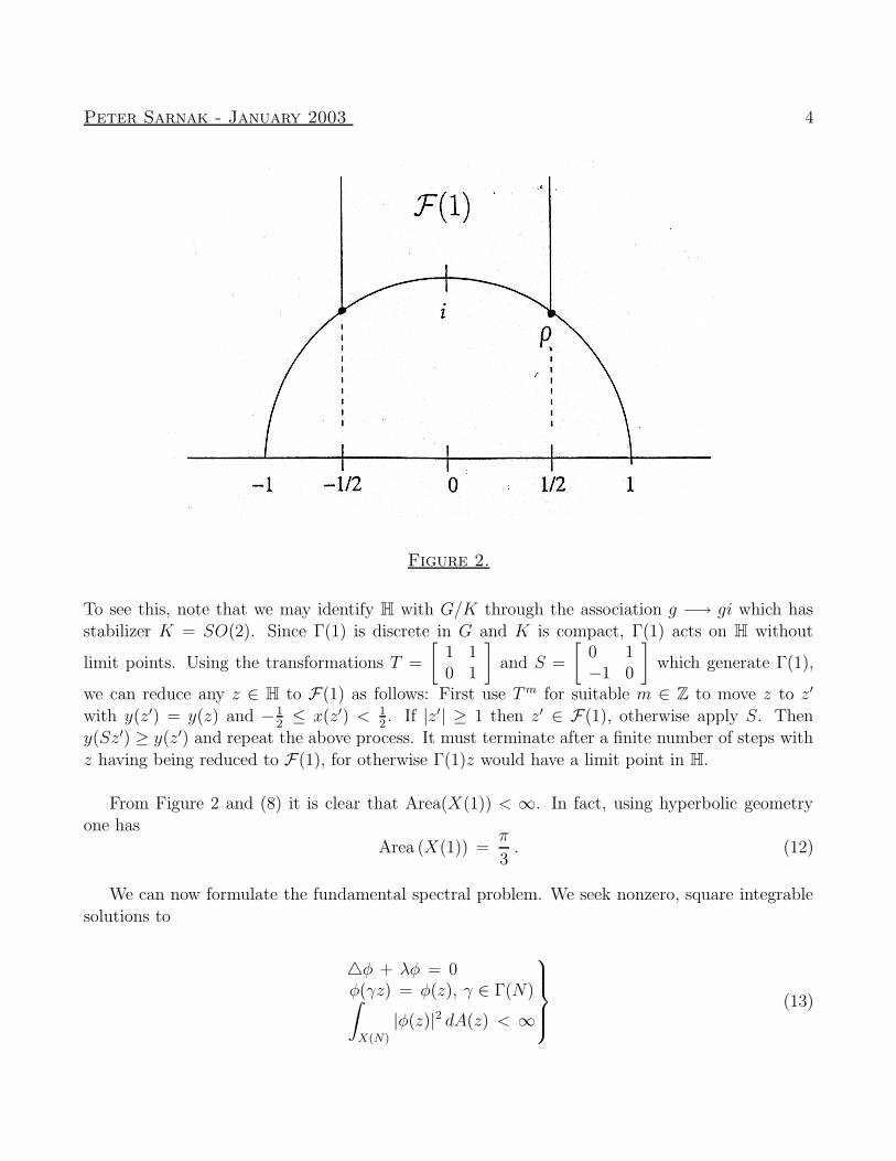
This can be seen from the standard fundamental domain F(1) for the action of Γ(1).


Figure 2.

To see this, note that we may identify H with G/K through the association g −→ gi which hasstabilizer K = SO(2). Since Γ(1) is discrete in G and K is compact, Γ(1) acts on H without

limit points. Using the transformations T =

[

1 10 1

]

and S =

[

0 1−1 0

]

which generate Γ(1),

we can reduce any z ∈ H to F(1) as follows: First use Tm for suitable m ∈ Z to move z to z′

with y(z′) = y(z) and − 12≤ x(z′) < 1

2. If |z′| ≥ 1 then z′ ∈ F(1), otherwise apply S. Then

y(Sz′) ≥ y(z′) and repeat the above process. It must terminate after a finite number of steps with

z having being reduced to F(1), for otherwise Γ(1)z would have a limit point in H.

From Figure 2 and (8) it is clear that Area(X(1)) < ∞. In fact, using hyperbolic geometryone has

Area (X(1)) =π

3. (12)

We can now formulate the fundamental spectral problem. We seek nonzero, square integrable

solutions to

4φ + λφ = 0φ(γz) = φ(z), γ ∈ Γ(N)∫

X(N)

|φ(z)|2 dA(z) < ∞

(13)


The numbers2 0 = λ0 < λ1 ≤ λ2 ≤ . . . for which (13) has a solution turn out to be discrete andform the (discrete) spectrum of X(N). The corresponding eigenfunctions φλ(z) are also of much

interest. The only obvious eigenfunction is the constant function for which λ = λ0 = 0. We calla solution to (13) a Maass form after Maass who first introduced them3. Their existence is by no

means obvious - see Section 2.

Intensive numerical investigations[He1] [St] have determined the first 10,000 eigenvalues for

X(1). The first few being: 0, 91.14. . ., 148.43. . ., 190.13. . ., 206.16. . . . They are respectively even,

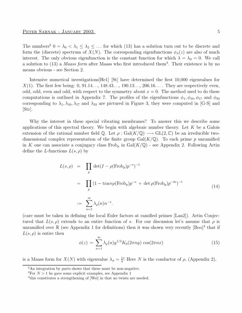
odd, odd, even and odd, with respect to the symmetry about x = 0. The method used to do thesecomputations is outlined in Appendix 7. The profiles of the eigenfunctions φ1, φ10, φ17 and φ33

corresponding to λ1, λ10, λ17 and λ33 are pictured in Figure 3, they were computed in [G-S] and[Str].

Why the interest in these special vibrating membranes? To answer this we describe some

applications of this spectral theory. We begin with algebraic number theory. Let K be a Galoisextension of the rational number field Q. Let ρ : Gal(K/Q) −→ GL(2,C) be an irreducible two-

dimensional complex representation of the finite group Gal(K/Q). To each prime p unramifiedin K one can associate a conjugacy class Frobp in Gal(K/Q) - see Appendix 2. Following Artin

define the L-functions L(s, ρ) by

L(s, ρ) =∏

p

det(I − ρ(Frobp)p−s)−1

=∏

p

(1 − traceρ(Frobp)p−s + det ρ(Frobp)p

−2s)−1

:=

∞∑

n=1

λρ(n)n−s.

(14)

(care must be taken in defining the local Euler factors at ramified primes [Lan2]). Artin Conjec-

tured that L(s, ρ) extends to an entire function of s. For our discussion let’s assume that ρ isunramified over R (see Appendix 1 for definitions) then it was shown very recently [Boo]4 that if

L(s, ρ) is entire then

φ(z) =∞∑

n=1

λρ(n)y1/2K0(2πny) cos(2πnx) (15)

is a Maass form for X(N) with eigenvalue λφ = 14! Here N is the conductor of ρ, (Appendix 2),

2An integration by parts shows that these must be non-negative.3For N > 1 he gave some explicit examples, see Appendix 14this constitutes a strengthening of [Wei] in that no twists are needed.


λ1 = 91.12 . . .

λ10 = 379.90 . . .

λ17 = 541.27 . . .

λ33 = 916.52 . . .

Figure 3

The 1st, 10th, 17th and 33rd eigenfunctions for the modular group. They are all odd with respect

to the symmetry z −→ −z.

and K0(y) is the Bessel function. The latter may be defined by

Kν(y) =

∫ ∞

0

e−y cosh t cosh(νt) dt (16)


and it satisfies

K ′′ν +

1

yK ′ν +

(

1 − ν2

y2

)

Kν = 0 . (17)

Observe that if

ψ(z) =∞∑

n=1

a(n) y1/2Kit (2πny) cos(2πnx) (18)

for any coefficients a(n), then

4ψ +

(

1

4+ t2

)

ψ(z) = 0. (19)

The important feature in (15) is the Γ(N) invariance.

Thus, according to Artin’s Conjecture even Galois representations (Appendix 2) give rise to

Maass forms with eigenvalue 14. Similarly, odd ones give rise to holomorphic forms of weight 1,

see [Se]. If the image of ρ in PGL(2,C) (which being finite must according to Klein [Kl] be one

of the following; dihedral, tetrahedral,octahedral or icosahedral) is not icosahedral, then the ArtinConjecture is true. The most difficult cases being the tetrahedral and octahedral ones which were

established in [La1] and [Tu].5 The proof makes crucial use of the spectral theory via use of thetrace formula (Appendix 3) to establish cyclic base change. The latter gives a precise relation

between the automorphic (in particular Maass) spectrum over a number field L and that of acyclic extension K of L.

It is believed that conversely any Maass form φ with eigenvalue λφ = 14

must correspond to aneven Galois representation as above. In [Sa1] it is shown that if φ(z) is a Maass form for some

X(N) and has integer coefficients in its Fourier expansion (18) then in fact λφ = 14

and φ comesfrom a Galois representation of dihedral or tetrahedral type. The proof of this result relies on

recent advances [K-S] on the functorial lifts sym3 : GL(2) −→ GL(4), see Appendix 1.

We turn to some applications of this spectral theory to problems in analytic number theory.

In these it is the entire spectrum that usually enters. For example, let λρ(n) be the coefficients in(14) or for that matter the coefficients of any holomorphic or Maass form. For integers ν1, ν2, h ≥ 1

consider the Dirichlet series

5For recent progress for ρ odd and icosahedral (see [B-D-S-T]).


D(s, ν1, ν2, h) =∑

ν1n−ν2m=h

λρ(n)λρ(m) (ν1n + ν2m)−s (20)

The series converges absolutely for <(s) > 1. As was first noted in [Sel2] and is explained inAppendix 6, D has an analytic continuation to <(s) ≥ 1

2with possible poles at s = 1

2+ itφ where

0 6= λφ = 14

+ t2φ is an eigenvalue of 4 on X(ν1ν2N). Notice that if λφ ≥ 14

(see Section 3) thenin fact D(s, ν1, ν2, h) is analytic in <(s) > 1

2. The latter represents a substantial (“square root”)

cancellation in the following smooth sums: If ψ ∈ C∞0 (0,∞) and ε > 0 there is Cε,ψ such that

∣

∣

∣

∣

∣

∑

ν1n−ν2m=h

ψ

(

ν1n+ ν2m

Y

)

λρ(n)λρ(m)

∣

∣

∣

∣

∣

≤ Cε,ψY12+ε , as Y −→ ∞. (21)

Cancellation in such and related arithmetical sums is at the heart of many of the applications of

the Maass form spectral theory. We mention a couple.

1. Equidistribution of roots:

Let f(x) ∈ Z[x] be an irreducible polynomial over Q. If K is the splitting field for f then

Frobp and (14) are concerned with how f(x) factors mod p, for different primes p. Let0 ≤ xj(p) ≤ p − 1, j = 1, 2, . . . , νp, νp ≤ deg f be the roots of f(x) ≡ 0(p) if there are any.

Numerical experiments suggest that xj(p)/p, j = 1, . . . , νp, p ≤ X become equidistributedin [0, 1] as X −→ ∞. In [D-F-I] and [To] it is shown that this is indeed the case when f is

of degree 2. That is for 0 ≤ α ≤ ß ≤ 1,

#p ≤ X, j ≤ νp| xj(p)

p∈ [α, ß]

#p ≤ X, j ≤ νp−→ ß − α, asX −→ ∞ . (22)

2. Hilbert’s eleventh problem:

This asks about the representations of integers in a number field K (respectively of elements

in K) by an integral (respectively K rational) quadratic form F (x1, x2, . . . xn) in n-variables.For the case of representability of members of K by a form F with coefficients in K this

was resolved by Hasse [Ha]. He showed that F (x) = n has a solution x ∈ Kn, m ∈ Kiff F (x) = m has a solution over Kv for every completion Kv of K. This is called a local

to global principle. The case of integral representations is apparently more difficult. Afterworks of Minkowski, Siegel and others, an appropriate local to global principle for intergral

forms in 4 or more variables was established in [Kne]. In the most interesting case thatthe form is definite then the local to global principle applies when m is large. For two

variables there is in general no such local to global principle. The case of 3 variables was

resolved recently in [Co-PS-S] where a local to global principle is proven. There is an added


caveat of the result being ineffective and that for 3 variables there may be a finite numberof quadratic exceptional sequences [D -SP], [SP]. An interesting application of the above is

the determination of which integers m in K are a sum of 3 squares of integers of K. Animportant ingredient in [Co-PS-S] is the analysis of the Maass form spectrum and especially

the low energy eigenvalues for Hilbert modular manifolds (for an example of these see theend of Section 4), which are the natural generalizations of the X(N)’s for K.

We hope that the above examples convince you of the central role that the spectrum of X(N)plays in number theory. In the analytic aspects it is the low energy spectrum that is critical. In

Section 3 we discuss this aspect of the spectrum. The study of the large eigenvalues for a given Xis also of interest, especially as a problem in mathematical physics. The limit λ −→ ∞ is the so

called semi-classical limit. In our case of a hyperbolic surface X, we are dealing with a quantizationof a classically chaotic Hamiltonian and for these (unlike the case of a completely integrable

Hamiltonian) the relation in the semi-classical limit between the classical and quantum mechanicsis not well understood. We discuss these issues as well as some recent decisive breakthroughs for

the surfaces X(N), in Section 4.

§2. Existence

We first recall a fundamental result of Weyl. Let Ω ⊂ R2 be a compact planar Euclidian domainwith smooth boundary ∂Ω. The eigenvalue problem for the usual Laplacian 4 = ∂2

∂x2 + ∂2

∂y2on Ω

with Dirichlet boundary conditions is

4φ(z) + λφ(z) = 0 for z ∈ Ω

φ∣

∣

∂Ω= 0 .

Let NΩ(R) be the number of such eigenvalues λ counted with multiplicity, with λ ≤ R. Weyl’sresult, known as Weyl’s law asserts that

NΩ(R) ∼ Area(Ω)

4πR, as R −→ ∞ .

The result has been generalized to Riemannian manifolds of any dimension. For many, the favored

modern means of proving this law is by analyzing the small time asymptotics of the heat kernel onR × Ω [Mc-Si]. The sharpest forms of the remainder terms for such Weyl asymptotics are gotten

by analyzing the propogation of singularities for the wave kernel [Du-Gu].

We return to our setting of finite area hyperbolic surfaces. Since the spaces X(N) are notcompact it is not at all clear that there are any solutions to (13) with λ > 0. The discrete

spectrum that we seek lies embedded in the continuous spectrum making these eigenvalues very

difficult to isolate analytically. The theory of Eisenstein series and their analytic continuation


developed in [Sel1] for a general hyperbolic surface XΓ = Γ\H, furnishes the continuous spectrum.The latter consists of the interval [ 1

4,∞) with multiplicity the number of cusps of XΓ. The constant

term in the Fourier expansion of the Eisenstein series (see (43)), φΓ(s) (called the determinant ofthe scattering matrix in [L-P] or the intertwining operator in [Sh]) is meromorphic in C. Its only

poles in <(s) ≥ 12

are in (12, 1] and the residues at these poles furnish solutions to (13) called the

residual spectrum of X. The poles of φΓ(s) in <(s) < 12

yield resonances for the problem (13).

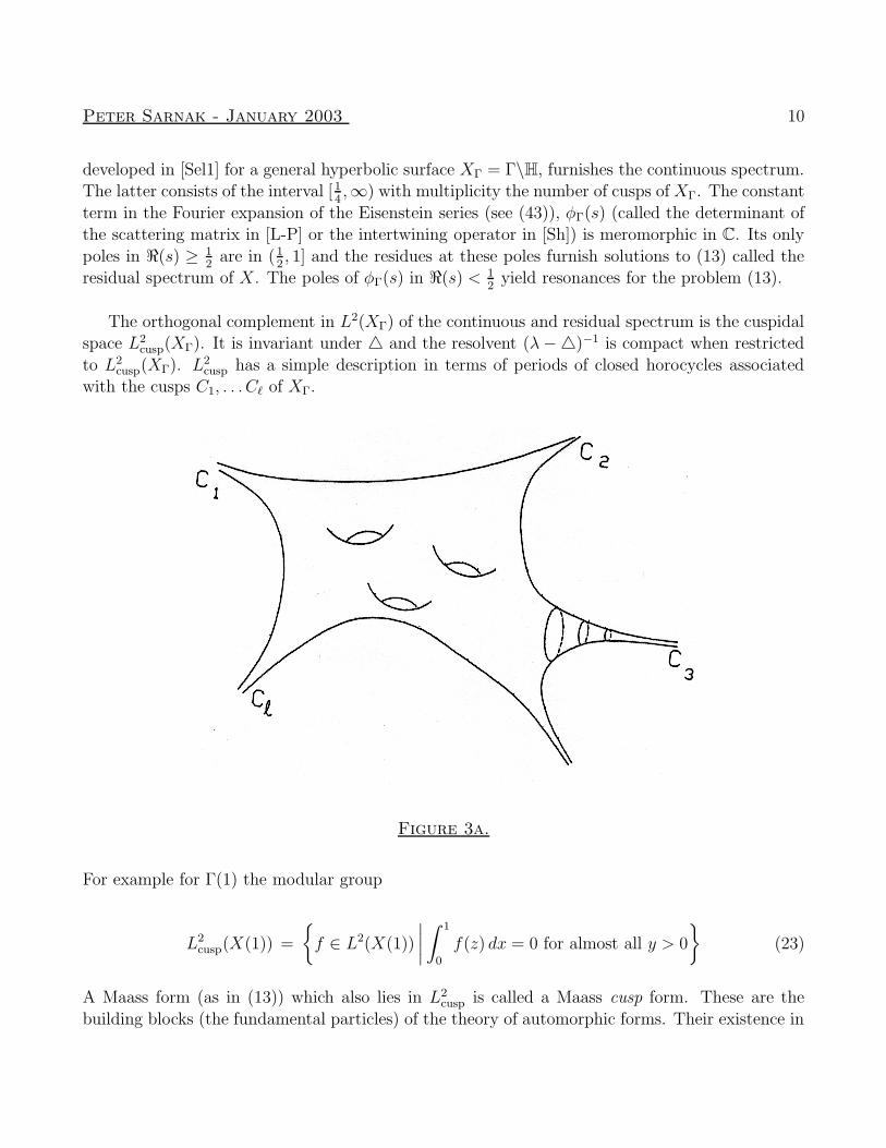
The orthogonal complement in L2(XΓ) of the continuous and residual spectrum is the cuspidalspace L2

cusp(XΓ). It is invariant under 4 and the resolvent (λ−4)−1 is compact when restricted

to L2cusp(XΓ). L2

cusp has a simple description in terms of periods of closed horocycles associatedwith the cusps C1, . . . C` of XΓ.

Figure 3a.

For example for Γ(1) the modular group

L2cusp(X(1)) =

f ∈ L2(X(1))

∣

∣

∣

∣

∫ 1

0

f(z) dx = 0 for almost all y > 0

(23)

A Maass form (as in (13)) which also lies in L2cusp is called a Maass cusp form. These are the

building blocks (the fundamental particles) of the theory of automorphic forms. Their existence in


this setting is tied to the size of L2cusp(X(1)). Whether L2

cusp(X) 6= 0 for a general hyperbolic Xis by no means obvious. An interesting discussion in terms of integral geometry is given in [Lax].

One of the early triumphs of the trace formula (Appendix 3) developed in [Sel1] was the proof

that the modular surfaces X(N) carry an abundance of Maass cusp forms. For these surfaces thefunctions φΓ(N)(s) may be expressed in terms of Dirichlet L-functions (Appendix 1). For example

for Γ(1)

φΓ(1)(s) =Λ(2s− 1)

Λ(2s)(24)

with Λ(s) as in ( 4 ). In particular, φΓ(N)(s) has no poles in(

12, 1)

so that in these cases there isno residual spectrum (besides λ = 0) and any solution of (13) with λ > 0 is automatically a cusp

form. For the general XΓ, the trace formula provides a Weyl like law for counting asymptoticallythe sum of the cuspidal spectrum and the continuous spectrum - the latter through the winding

of the unitary quantity φΓ(s) for <(s) = 12

(Appendix 3). In the case of a modular surface theexpression of φΓ(N)(s) in terms of L-functions allows one to show that the contribution of the

continuous spectrum to this Weyl law is negligible. That is, for X(N) it is shown in [Sel1](seeAppendix 3) that

N cuspΓ(N) (λ) :=

∑

0<λj≤λ1 ∼ Area X(N)

4πλ, as λ −→ ∞ . (25)

Thus, solutions to (13) exist and in abundance! We call a surface X essentially cuspidal if (25)

holds.

It is interesting6 from many points of view to understand when solutions to (13) exist, forthe more general hyperbolic surface X. Contrary to early beliefs it appears now that essential

cuspidality is limited to special arithmetic surfaces! We review briefly these developments. In thepapers [P-S1],[P-S2],[P-S3], the behavior of the discrete spectrum is studied when Γ undergoes a

deformation. Fix N and let T (Γ(N)) be the deformation space (Teichmuller space) of continuousdeformations of Γ(N) as a discrete subgroup of cofinite area in SL(2,R), that is as a hyperbolic

surface. The cotangent space to T (Γ(N)) at Γ(N) may be naturally identified with the space ofholomorphic quadratic differentials on X(N) (here the analytic structure of X(N) is exploited)

with suitable behavior at the punctures [Be]. Using the uniformization X(N) = Γ(N)\H thiscotangent space can be realized as the space of holomorphic cusp forms Q of weight 4 for Γ(N).

That is:6This is especially relevant in higher dimensions where the only understanding of φΓ(s) comes from spectral

theory [La3].


• Q(z) is holomorphic in H

• Q(

az+bcz+d

)

= (cz + d)4Q(z) for

[

a bc d

]

∈ Γ(N)

• Q vanishes at the cusps.

(26)

Unlike the issue of Maass cusp forms, the dimension of the space of holomorphic cusp forms ofweight 4 on any surface X, is determined purely in terms of the topology of X via the Riemann-

Roch formula.

Let Xt be a real analytic curve in T (Γ(N)) with X0 = X(N) and with tangent vector at t = 0

given by Q(z) as above. In order to investigate the behavior of the spectrum under deformationdefine the singular set σ(X), to be the numbers 1

2+ itj (with multiplicities) if λj = 1

4+ t2j is an

eigenvalue of 4 on XΓ, together with the poles ρj (again with order) of φΓ(s) in <(s) < 12. The

multiplicity of the point s = 12

as a member of σ(X) requires a special definition [P-S3]. Note that

σ(X)∩ s|<(s) ≥ 12 consists of points located in <(s) = 1

2 ∪ (1/2, 1]. In [P-S3] it is shown that

σ(Xt) is an algebroid function of t. That is, branches ρj(t) may be chosen so as to be analytic int or at worst to have algebraic singularities locally. Now, suppose that 1

2+ itj, tj > 0 is a simple

point in σ(X(N)) corresponding to a Maass form φj. Let ρj(t) be its corresponding deformation.Either <(ρj(t)) ≡ 1

2or ρj(t) moves into <(s) < 1

2. In the latter case the cusp form φj is dissolved

under the deformation into a pole of φΓt(s). In [P-S3] the following “Fermi Golden rule”7 is proven:

d2

dt2<(ρj(t))

∣

∣

∣

∣

t=0

= −c(tj)∣

∣

∣

∣

L

(

1

2+ itj, Q× φj

) ∣

∣

∣

∣

2

. (27)

Here c(tj) > 0 and L(s,Q × φj) is the Rankin-Selberg L-function of Q and φj (see Appendix 1

for a definition). The proof of (27) relies in a crucial way on the scattering theory (specificallythe semi-group Z(t)) developed in [L-P]. A similar formula for the movement of sj = 1

2(ie tj = 0

above), when movement to the right is also possible, is developed in [Pe].

The dissolving condition (27) boils down to a vanishing question about a special value of a zeta

function. Note that the special value is on the critical line for this function so that the vanishingdoes not violate the corresponding Riemann Hypothesis (Appendix 1). Starting with [D-I] there

have been a series of results concerning the non-vanishing of these numbers L( 12

+ itj, Q × φj),|tj| ≤ T . In [Lu] it is shown that a positive proportion of these numbers are not zero, as T −→ ∞.

Note that once a Maass form φj is dissolved then it is a pole (or resonance) for all but countably

7See [Si] for a discussion of this terminology in the context of Helium-like atoms.


many values of t. Thus generically in T (Γ(N)) it is dissolved into a pole. There is a technicaldifficulty in this analysis in the case that 1

2+ itj is a multiple eigenvalue. Specifically degenerate

perturbation theory leads to a much less tractable (in terms of L-functions) formula for the GoldenRule. This leads us to the issue of the possible multiplicities of the eigenvalues of X(N). This has

proven to be an embarrassingly difficult problem - see Section 4. It is believed that the multiplicitym(λ) of an eigenvalue λ of X(N) should be uniformly bounded (here N is fixed). Assuming this

then the above analysis leads to the conclusion that for the generic Γ ∈ T (Γ(N)), XΓ is not

essentially cuspidal. The dissolving condition (27) led to the following Conjectures [Sa2]:

Conjecture 1:

(a) The generic Γ in a given Teichmuller space of finite area hyperbolic surfaces is not essentially

cuspidal.

(b) Except for the Teichmuller space of the once punctured torus, the generic Γ has only a finitenumber of discrete eigenvalues.

The reason for omitting the once punctured torus is that this Teichmuller space has a persistentsymmetry of order 2 which leaves the continuous spectrum invariant. The functions which are odd

with respect to this symmetry constitute half of L2(XΓ) and these functions are all cuspidal. Inthe context of deforming XΓ in the infinite dimensional space of all Riemannian metrics which are

conformal to XΓ, part (b) is known and was established in [Co2].

Remarkable further progress on the above Conjecture was made in the series of papers [Wo1][Wo2].

Instead of considering regular deformations in T (Γ) he follows special deformations Γt to the bound-ary of T (Γ). This is a formidable task, being an analysis of eigenvalues embedded in the continuum

for a very singular perturbation. The payoff of going to the boundary is well worth it. The pointbeing that the key dissolving condition (27) takes a similar form with L

(

12

+ itj, Q× φj)

being

replaced by L(

12

+ itj, E4 × φj)

, where E4 is the Eisenstein series:

E4(z) =∑

γ∈Γ∞\Γ(N)

(cz + d)−4

Γ∞ =

(

1 Nm0 1

) ∣

∣

∣

∣

m ∈ Z

.

(28)

This holomorphic weight 4 Eisenstein series generates a singular deformation at the boundaryof T . The theory of such singular deformations (of infinite energy) was developed in [W]. The

advantage of E4 over Q is that the degree 4 L-function L(s, E4 × φj) factors into the two degree


2 L-functions (Appendix 1) L(s + 1, φj) L(s − 1, φj). Thus evaluation at s = 12

+ itj ensuresthe non-vanishing of this product since L-functions can only vanish in 0 < <(s) < 1 or at the

trivial zeroes! Unfortunately, there is still the caveat of the multiplicity issue. In fact, the analysisneeded to handle this very singular perturbation requires the strongest multiplicity Conjecture

(see Section 4).

Theorem 1 [Wo2]:

Assume that the cuspidal Maass spectrum (of new and old forms) for X(2) is simple, then part

(a) of Conjecture 1 is true.

One may ask if there is a characterization of those Γ which have many Maass cusp forms?In [Sa2] the question of the relation to arithmeticity is raised. The simplest case to explain this

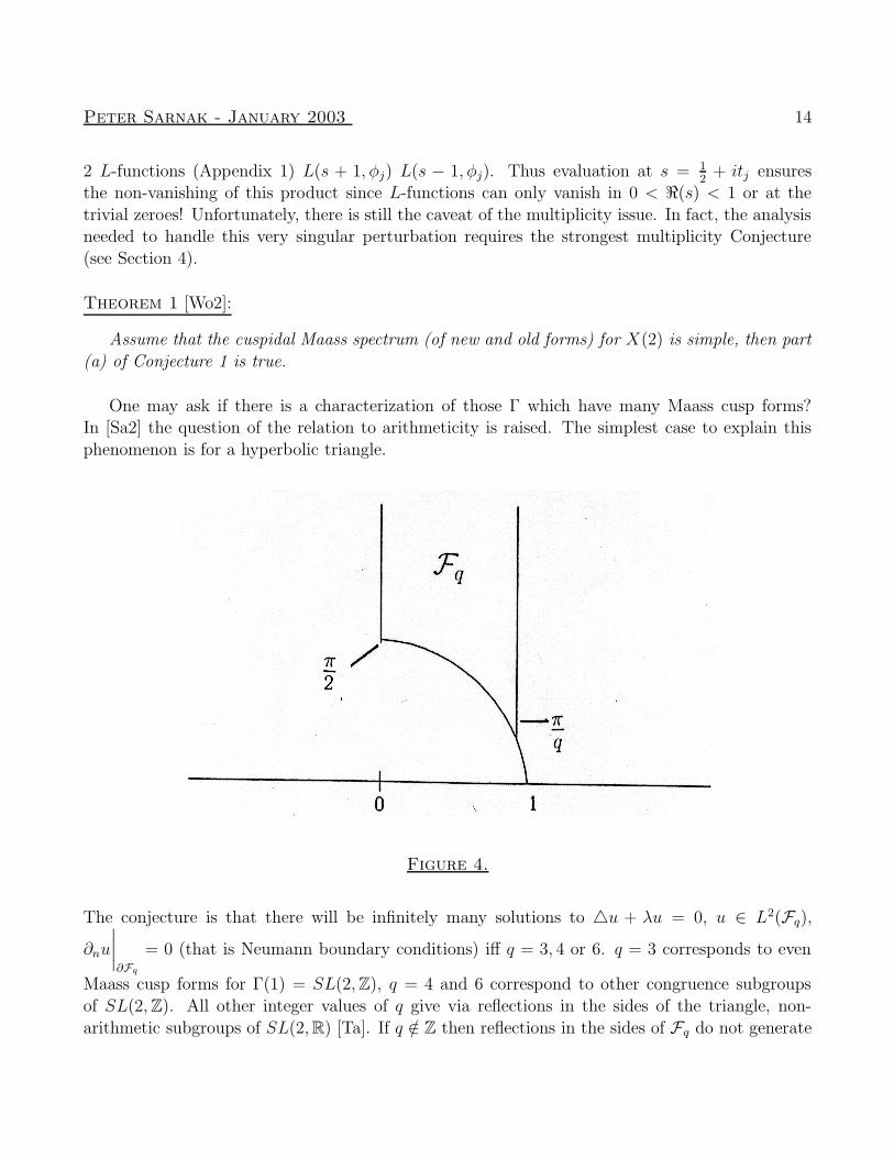
phenomenon is for a hyperbolic triangle.

Figure 4.

The conjecture is that there will be infinitely many solutions to 4u + λu = 0, u ∈ L2(Fq),

∂nu

∣

∣

∣

∣

∂Fq

= 0 (that is Neumann boundary conditions) iff q = 3, 4 or 6. q = 3 corresponds to even

Maass cusp forms for Γ(1) = SL(2,Z), q = 4 and 6 correspond to other congruence subgroups

of SL(2,Z). All other integer values of q give via reflections in the sides of the triangle, non-

arithmetic subgroups of SL(2,R) [Ta]. If q /∈ Z then reflections in the sides of Fq do not generate


a discrete subgroup of SL(2,R) but the above eigenvalue problem for the triangle makes sense.This conjecture about these triangles has been checked numerically in [He2]. For example for

q = 5, 7 and 8 no eigenvalues were found for 0 < λ < 3600. In [Ju] the dissolving condition (26)at “q = ∞” is developed using a similar singular perturbation method to [Wo1]. He shows that

subject to the same hypothesis as in Theorem 1, Fq has only a finite number of eigenvalues for allbut a countable set of q.

By looking at more general surfaces XΓ we have learned something about the Maass forms φ for

X(N). They are very fragile and special objects and even their existence is tied to the arithmeticof Γ(N). We end this Section by pointing out that some higher rank cases of essential cuspidality

have been established recently. For X = SL(3,Z)\SL(3,R)/SO(3) in [Mi] and for the generalcongruence quotient of SL(n,R)/SO(n) in [Mu].

§3. Low Energy Spectrum

We mentioned in Section 1 in connection with Galois representations the importance of the

eigenvalue λ = 14

forX(N). It was also noted that in analytic applications an eigenvalue 0 < λφ <14

would have a drastic impact on the cancellations in the sums (21). The question of the smallestnon-zero eigenvalue for these surfaces is one of the major problems in the subject. Let λ1(X)

denote the next to smallest (the smallest is λ0 = 0) eigenvalue of 4 on L2(X).

Conjecture 2 [Sel1]: For N ≥ 1, λ1(X(N)) ≥ 14.

We call this the Selberg-Ramanujan Conjecture since it was first formulated in [Sel1] but todaywe understand it as part of the general Ramanujan Conjectures [La2].

Comments:

1. As noted in Section 2 there is no residual spectrum for X(N) so we could take for λ1(X(N))

the smallest eigenvalue of a Maass cusp form for X(N). The continuous spectrum is the

interval [14,∞), so we may also formulate the conjecture variationally as follows:

For any f ∈ C∞0 (X(N)), that is smooth and compactly supported and for which

∫

X(N)

f(z) dA(z) = 0

we have

∫

X(N)

|OHf(z)|2 dA(z) ≥ 1

4

∫

X(N)

|f(z)|2 dA(z). (29)


2. Another reason for the relevance of the number 14

is that the spectrum of 4 on the universalcovering L2(H) is [1

4,∞). To see that λ0(H) ≥ 1

4let f ∈ C∞

0 (H). Following [Mc] we have

12

∫ ∞

0

f 2(z)dy

y2=

∫ ∞

0

fy(z) f(z)dy

y

≤(∫ ∞

0

(fy(z))2 dy

)1/2 (∫ ∞

0

f 2(z)dy

y2

)1/2

.

Hence

1

4

∫ ∞

0

f 2(z)dy

y2≤∫ ∞

0

| fy(z)|2 dy ≤∫ ∞

0

|Of |2 dy.

Integrating with respect to x yields

1

4

∫

f2(z) dA(z) ≤

∫

|Of |2 dxdy =

∫

|OHf |2 dA(z).

3. It is not difficult to show that the cuspidal spectrum of 4 becomes dense in [ 14,∞) as

N −→ ∞. Thus Conjecture 2 if true is sharp.

4. Conjecture 2 is somewhat surprising. After all the surfaces X(N) have their area and genus

going to infinity with N . This might lead one to expect that the low “overtone” λ1(X(N))should go to zero. That this is not the case is combinatorially very powerful. The optimally

highly connected but sparse, Ramanujan Graphs [L-P-S] and [M], are constructed via similarcongruence quotients of the p-adic groups PGL(2,Qp).

5. The assumption that Γ is a congruence subgroup of SL(2,Z) cannot be dropped. In [Sel1]

it is shown that given ε > 0 there is a cyclic cover XΓ′ of X(2) for which λ1(XΓ′) < ε. Inview of the results below towards Conjecture 2 it follows that for ε small Γ′ cannot contain

Γ(M) for any M . These Γ′ are finite index subgroups of SL(2,Z) which are not congruencesubgroups.

6. Conjecture 2 is known for N ≤ 17 [Hu]. The combinational topological method used therewhen successful establishes that λcusp

1 (X(N)) > 14. In view of the presence of Galois repre-

sentations this method breaks down for large N .

In [Sel2] the bound λ1(X(N)) ≥ 316

was established. It is already very useful in many applica-

tions. By a completely different method[Ge-Ja] showed that λ1(X(N)) > 316

. Their approach isbased on the symmetric square sym2 : GL(2) −→ GL(3) functorial lift (see Appendix 1). They then


invoke local representation theoretic bounds concerning generic representations of GL(3,R), [Ja-Sh]. In [L-R-S] global bounds towards the general Ramanujan Conjectures on GL(m,A ) m ≥ 2,

are established using families of L-functions. Combining this for the case of GL(3) together withsym2 as above leads to λ1(X(N)) ≥ 21

100. Recently, the functorial lifts sym3 : GL(2) −→ GL(4)

and sym4 : GL(2) −→ GL(5) were established [K-S][K]. Combining these with the methods fromfamilies of L-functions one obtains

Theorem 2 [Ki-Sa]: λ1(X(N)) ≥ 9754096

= 0.238 . . .

This is getting close to 14

but it is also close to the limit of these methods. The functorial lifts

sym3 and sym4 are based on the continuous spectrum (Eisenstein series) on exceptional groupsincluding E8. What can be done this way terminates with the finite list of exceptional groups. We

see clearly here that other groups and symmetric spaces play a central role in understanding GL(2)(that is essentially the upper half-plane). We note that if the general Functoriality Conjectures

concerning the automorphic lifts symk : GL(2) −→ GL(k+1), k ≥ 1 are valid then so is Conjecture2 [La2].

Conjecture 2 is concerned with the bottom of the spectrum of the Laplacian 4 on L2cusp(X(N)),

that is the spectrum at the “archimedean” place. There is a similar conjecture for each prime p for

the corresponding Hecke operator Tp. The surfaces X(N) carry algebraic correspondences whichgive rise to the family of Hecke operators. For (n,N) = 1 define Tn by

Tn f(z) =1√n

∑

ad=nb mod d

f

(

az + b

d

)

. (30)

These are closely related to the cosets of the finite index subgroups

(

n 00 1

)

Γ(N)

(

n 00 1

)−1

∩ Γ(N)

of Γ(N). The linear transformation Tn maps L2(X(N)) −→ L2(X(N)).

The Tn’s are normal, they commute with each other and with 4 and leave L2cusp(X(N))

invariant. (31).


The Ramanujan Conjectures for these Tp’s asserts the following

∥

∥

∥

∥

Tp

∣

∣

∣

∣

L2cusp(X(N))

∥

∥

∥

∥

≤ 2. (32)

One can show that the above norm is at least 2 so that (32) is equivalent ‖ Tp|L2cusp(X(N)) ‖= 2.

The trivial bound (from (29)) for ‖ Tp ‖ is

‖ Tp ‖≤ p12 + p−

12 . (33)

The functorial techniques [K] apply to these finite places as well and if one combines them with

the L-function techniques of [Du-Iw] one obtains the following very useful bounds [Ki-Sa]

‖ Tp|L2cusp(X(N)) ‖≤ p

764 + p−

764 . (34)

A unification and clarification of the theory of the spectrum of 4 and of Tp is provided by therepresentation theoretic description of the subject. That is the spectral decomposition of the right

regular action of GL(2,A ) on GL(2,Q)\GL(2,A ) where A is the adele group of Q [Ge]. Thislanguage is indispensable for many purposes. We have avoided it in order to keep our discussion

as self-contained and elementary as possible. A recent discussion of these adelic spectral problemsfor more general groups can be found in [Cl].

§4. High Energy Spectrum

In this Section we examine the solutions (13) for λ large. For this limit the case of X(1) already

contains the key features so for the most part we will concentrate on X(1). Probably the simplestand most basic question concerning the eigenvalues of X(1) was raised in [Ca] where the first

attempts to numerically compute the eigenvalues were carried out.

Conjecture 3 [Ca]: The (cuspidal) spectrum of 4 on X(1) is simple.

The main evidence for this are the numerical computations [St] which confirm the Conjecturefor the first 10,000 eigenvalues. Let mX(1)(λ) be the multiplicity of the eigenvalue λ. The best

known bounds for m(λ) are rather poor. They are derived from the trace formula by analyzing theremainder term in the Weyl asymptotics (25). The difficulty in all questions involving the large

λ limit is that when localizing a test function in the trace formula (Appendix 3) near λ one isfaced on the dual side (via Fourier Transform) with an exponential in λ number of terms involving

closed geodesics. It is then very problematic to establish suitable cancellations in these sums over


the closed geodesics. All that seems possible is to treat these sums trivially and after optimizingthe choice of test functions one obtains a bound for mX(λ) for the general hyperbolic surface X.

limλ−→∞

mX(λ) log λ√λ

≤ Area(X)

2. (35)

For X(1) one can obtain square root cancellation in the relevant sums by using the relative trace

formula [Ku] which involves Kloosterman sums instead of closed geodesics. This leads to a modestimprovement over (35) for X(1) [Sa3];

limλ−→∞

mX(1)(λ) logλ√λ

≤ Area(X(1))

4=

π

12. (36)

It is an important problem to improve this bound (36). In my youth I would have been impressed

with the bound mX(1)(λ) = 0(λ12−δ) for some δ > 0. Today mX(1)(λ) = o

(√λ / logλ

)

looks good.

An interesting phenomenological fact about the spectrum of X(1) was noted in [St]. Consider

the numbers λj = λj/12 where λj are the eigenvalues of X(1). According to (25) the mean spacings

between the numbers λj is 1. The numerical experiments in [St] suggest that the consecutivespacings and for that matter any local spacing statistic behaves like random numbers would, or

as is often said - the local spacings statistics are “Poissonian”. More precisely, the consecutivespacings apparently obey the following law: For 0 ≤ α < ß <∞,

As N −→ ∞,#j ≤ N |λj+1 − λj ∈ [α, ß]

N−→

∫ ß

α

e−xdx . (37?)

This random behavior of the eigenvalues of X(1) is unexpected. To explain why so we recallthe interest that the spectrum of a hyperbolic surface has generated in mathematical physics.

Given x ∈ X and ξ ∈ Tx(X) a unit tangent vector and t ∈ R let (x(t), ξ(t)), ξ(t) ∈ Tx(t)(X),be the position and tangent vector after flowing for arc-length t from x in the direction ξ along

the corresponding geodesic. This flow Gt : S(X) −→ S(X) on the unit circle bundle to X is thegeodesic flow. It is a Hamilton flow. In terms of the uniformization X = Γ\H we can identify

S(X) with Γ\G, G = PSL(2,R) and Gt takes the form

ΓgGt−→ Γg

(

et/2 00 e−t/2

)

. (38)

Gt clearly preserves the Haar measure dg.


It is well known that the geodesic flow of a manifold of negative curvature is ergodic,8 Anosov,has positive Lyapunov exponents . . . . In short, it is a “chaotic” Hamiltonian. Now the eigenvalue

problem for 4 on XΓ corresponds to a quantization of this classically chaotic dynamics. The largeλ limit for this quantization is the same as the semi-classical limit ( −→ 0) of the quantum system.

Unlike the case of the quantization of a completely integrable Hamiltonian where the impact ofclassical invariant torri on the spectrum in the semi-classical limit is well understood [Laz], very

little can be said analytically in the chaotic case. The study of the semi-classical limit, specifically

the relation between the classical and quantum mechanics of a classically chaotic Hamiltonian goesby the name of Quantum Chaos.

One of the interesting suggestions that has emerged from many numerical investigations is that

the local spacing statistics of the eigenvalues of the quantization of a classically chaotic Hamiltonian

are modeled by the local spacing laws of the eigenvalues of a random matrix in a suitable matrixensemble. These laws are very different from the Poissonian laws that the spectrum of X(1)

exhibits. This then is the sense in which the spectrum of X(1) has unexpected statistics. No doubtthe reason for this anomaly is that 4 commutes with the geometrically defined Hecke operators

Tn in (30) (see also [Sa4]). Indeed, for the spectrum for the Dirichlet problem (which has discretespectrum only) for the triangles Fq in Figure 4, it is found numerically that for q 6= 3, 4, 6 (in

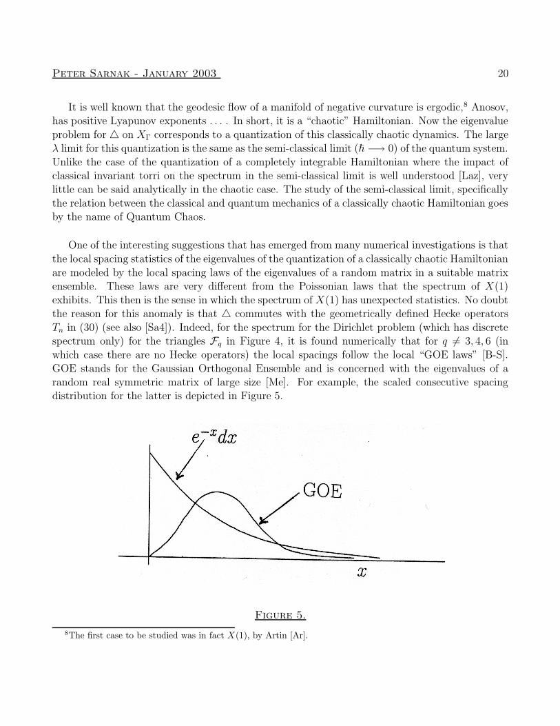
which case there are no Hecke operators) the local spacings follow the local “GOE laws” [B-S].GOE stands for the Gaussian Orthogonal Ensemble and is concerned with the eigenvalues of a

random real symmetric matrix of large size [Me]. For example, the scaled consecutive spacingdistribution for the latter is depicted in Figure 5.

Figure 5.

8The first case to be studied was in fact X(1), by Artin [Ar].


The density of the GOE consecutive spacing law vanishes to first order at x = 0 indicating thatthe eigenvalues of a random matrix repel each other and that the corresponding spectrum is rigid.

In contrast there are near degeneracies in the Poissonian laws. This phenomenology about thespectrum of X(1) is fascinating but very little can be proven.

We turn to the behavior of the eigenfunctions φλ for X(1) for which much is now known.

The basic issue is whether as λ −→ ∞ these eigenstates can localize or do they spread outevenly? For reasons similar to those mentioned above in connection the question of multiplicities,

it is very difficult to analyze the high energy eigenstates of the quantization of a classically chaoticHamiltonian. We next state the basic Conjectures asserting the non-localization of φλ for a general

hyperbolic X (possibly compact) as λ −→ ∞.

Conjecture 4: [I-S1]:

Fix X, K ⊂ X a compact (nice set) 9, 2 < p ≤ ∞ and ε > 0. There is c = c(p,K, ε) such that

(∫

K

|φλ(z)|p dA(z)

)1p

≤ cλε(∫

K

|φλ(z)|2 dA(z)

)12

.

Remarks:

1. This Conjecture asserts that the Lp norm on a nice compact set K ⊂ X (if X is compact

then take K = X) grow slower than any power of λ times the L2 norm. It quantifies thelack of localization of φλ. For the case of p = ∞ this Conjecture, if true, is quite deep since

it implies the classical Lindelof Hypothesis for the Riemann Zeta Function (Appendix 1).Also, for p = ∞ it implies that mX(λ) = Oε(λ

ε).

2. The λε factor is necessary when p = ∞ since in [I-S1] it is shown that ‖ φλ ‖∞ is not

uniformly bounded for certain compact X. Here (and henceforth) we will normalize φλ sothat ‖ φλ ‖2= 1.

There are some general interpolation bounds for the Lp norms of eigenfunctions φλ on a (fixed)general compact Riemannian surface X. In [So] it is shown that

‖ φλ ‖p λδ(p) , (39)

where δ(p) = 14− 1

p, for 6 ≤ p ≤ ∞ and δ(p) = 1

8− 1

4p, for 2 ≤ p ≤ 6. The proof of (39) uses

a construction of a parametrix for the wave equation via Fourier Integral Operators, combined

9for example K could be the closure of a nonempty geodesic ball.


with ideas from restriction theorems in Fourier Analysis [Ste]. The bound (39) is local in that itis derived on pieces of X directly. The global aspects of the geodesic motion do not enter. As a

local bound (39) cannot be improved since it is sharp on S2 with the round metric [So].

Another means to analyze the localization question is to examine the probability measures

µφ = |φλ(z)|2 dA(z) . (40)

Quantum mechanically this gives the probability distribution on X associated to being in the stateφλ. One can form a probability measure νφ on Γ\G, the micro-local lift of µφ to S(X), (Appendix

4) which projects to µφ and measures how φλ is distributed in phase space. For a ∈ C∞(Γ\G)νφ(a) measures the quantum observable Op(a) (see Appendix 4) when in the state φ.

Conjecture 5: [R-S] Quantum Unique Ergodicity

The measures νφ become equidistributed with respect to dg as λ −→ ∞. Precisely, if f ∈ C0(Γ\G)then

limλ−→∞

∫

Γ\Gf(g) dνφ(g) =

∫

Γ\Gf(g) dg := f

where dg is Haar measure on G normalized so that Vol(Γ\G) = 1.

Comments:

1. While this Conjecture seems reasonable enough, we point out that it contradicts some sug-

gestions that eigenstates in chaotic quantizations might concentrate on unstable periodicorbits, a phenomenon called scarring [Hel].

2. The name quantum unique ergodicity stems from there being in this context an analogueat the quantum level of ergodicity. Let φj be any orthonormal basis of L2(X) (if X is not

compact then we assume that X = X(N) and that φj is an orthonormal basis of L2cusp(X)).

In [Sh][Co][Ze] it is shown that if f ∈ C∞0 (Γ\SL(2,R)) then as λ −→ ∞

∑

λj≤λ|νφj

(f) − f |2 = o

∑

λj≤λ1

. (41)

In particular it follows that almost all, in the sense of density of the number of eigenvalues, ofthe νφ’s become equidistributed as λj −→ ∞. Recall that Gt being ergodic means that almost

all orbits of the flow become equidistributed as t −→ ∞. Thus the above is the quantum

analogue of the geodesic flow Gt being ergodic. For Gt however there are many singular


invariant measures (the most singular being arclength on an unstable periodic orbit). Thus,Conjecture 5 asserts that at the quantum level things are quite different in that all eigenstates

become equidistributed (a flow for which all orbits become equidistributed is called uniquelyergodic).

3. We call any weak limit of the measures νφλ, a quantum limit. Using some standard results

about propagation of singularities in the theory of Fourier Integral Operators one can show

that any quantum limit is Gt invariant - see Appendix 4. Conjecture 5 is equivalent to the

statement that the only quantum limit is dg.

For the general hyperbolic surface X little has been proven towards Conjectures 4 and 5. Howeverfor X(1) or more generally X(N) there has been some decisive progress. We restrict our discussion

to X(1). In view of (30) we can simultaneously diagonalize 4 and the operators Tn, n ≥ 1.

Henceforth we assume that our φλ is also a Hecke eigenform:

Tnφλ = λφ(n)φλ . (42)

Note that if Conjecture 3 is true then (42) is automatic. In any case it is the Maass-Hecke eigenform

that is of interest.

All these questions about the φλ’s for X(1) make sense for the continuous spectrum as well.

Explicitly the Eisenstein series E(z, s) for X(1) is defined as

E(z, s) =∑

γ∈Γ∞\Γ(1)

(y(γz))s for <(s) > 1 . (43)

E(z, s) extends meromorphically to C and is analytic on <(s) = 12. The continuous spectrum for

X(1) is furnished by the generalized eigenfunctions E(z, 12

+ it), t ≥ 0.

4E(

z,1

2+ it

)

+

(

1

4+ t2

)

E

(

z,1

2+ it

)

= 0 (44)

and of courseE(γz, s) = E(z, s) for γ ∈ Γ(1) .

Concerning Conjecture 4 for the case p = ∞ a sub-convex (or sub-interpolation) bound forX(1) is established in [I-S1]


‖ φλ ‖∞ λ5/24 . (45)

A similar bound for E(z, 12

+ it) is also proven.

In [L-S1] and [Ja] Conjecture 5 is proven for the continuous spectrum of X(1). Precisely, let µt be

the corresponding measure (of infinite mass)

µt = |E(

z,1

2+ it

) ∣

∣

∣

∣

2

dA(z) . (46)

Let νt be its micro-local lift to Γ(1)\G. Then for K1 and K2 (nice) compact subsets of Γ(1)\G wehave that

limt−→∞

νt(K2)

νt(K2)=

Voldg(K1)

Voldg(K2). (47)

For the measures νφ, Conjecture 5 has proven to be much more difficult to attack via the methodsof [L-S1]. In [R-S] it is shown that any quantum limit ν on Γ(1)\G cannot be supported on a finite

union of closed geodesics. In particular this strong form of scarring is not possible for X(1). In[B-L] a significant extension of this is given. They show that if ν is a quantum limit then it must

have positive entropy for the geodesic flow Gt.

An identity is derived in [Wa] which allows one to unify and make explicit the relation betweentriple products and special values of L-functions [H-K], [L-S1]. This allows one to convert some

of these questions concerning eigenfunctions to ones concerning the size of L-functions at specialpoints on their critical lines. The precise identity is as follows:

Let φ1, φ2, φ3 be three Maass (Hecke) eigenforms on X(1) normalized as before so that

‖ φj ‖2= 1. Then [Wa];

216 ·∣

∣

∣

∣

∫

X(1)

φ1(z)φ2(z)φ3(z) dA(z)

∣

∣

∣

∣

2

=π4 · Λ

(

12, φ1 × φ2 × φ3

)

Λ(1, sym2φ1) Λ (1, sym2φ2) Λ (1, sym2φ3)(48)

Here Λ(s, φ1×φ2 ×φ3) is the (completed) degree 8 L-function associated with φ1, φ2, φ3 and s = 12

is its central value [Appendix 1]. Λ(s, sym2φ) is the degree 3 L-function (Appendix 1) and s = 1is at the edge of the critical strip.

Using (48) one can reformulate Conjecture 5 in terms of estimates for L-functions. For example

the Lindelof Hypothesis (see [I-S2] and Appendix 1), which is a consequence of the Generalized


Riemann Hypothesis for these degree 8 L-functions, implies the following strong form of Conjecture5: For a fixed f ∈ C∞

0 (Γ(1)\G) and ε > 0

|νφλ(f) − f |

ε,fλ−1/4+ε . (49)

In fact, a “sub-convex” (Appendix 1) estimate for these L-functions would already establish Conjec-

ture 5. While there has been much progress on the general sub-convexity problem for L-functions,the general case at hand remains out of reach at the present time. We also note that the Lindelof

Hypothesis for these degree 8 L-functions implies Conjecture 4 with p = 4.

Recently, there have been a series of breakthroughs which lead to the solution of parts of the

Conjectures 4 and 5. These results are still being written up so that they should be regarded withappropriate caution until they have been independently confirmed.

Theorem 3 ([Sa-Wa], [Sp]):]

Fix ε > 0, then

(a) 10 ‖ φλ ‖4 ελε.

(b) For K ⊂ X(1) compact

(

∫

K

∣

∣

∣

∣

E

(

z,1

2+ it

) ∣

∣

∣

∣

4

dA(z)

)1/4

ε,K

(1 + |t|)ε(

∫

K

∣

∣

∣

∣

E

(

z,1

2+ it

) ∣

∣

∣

∣

2

dA(z)

)1/2

.

These establish Conjecture 4 for X(1) for 2 < p ≤ 4, for both the discrete and continuous

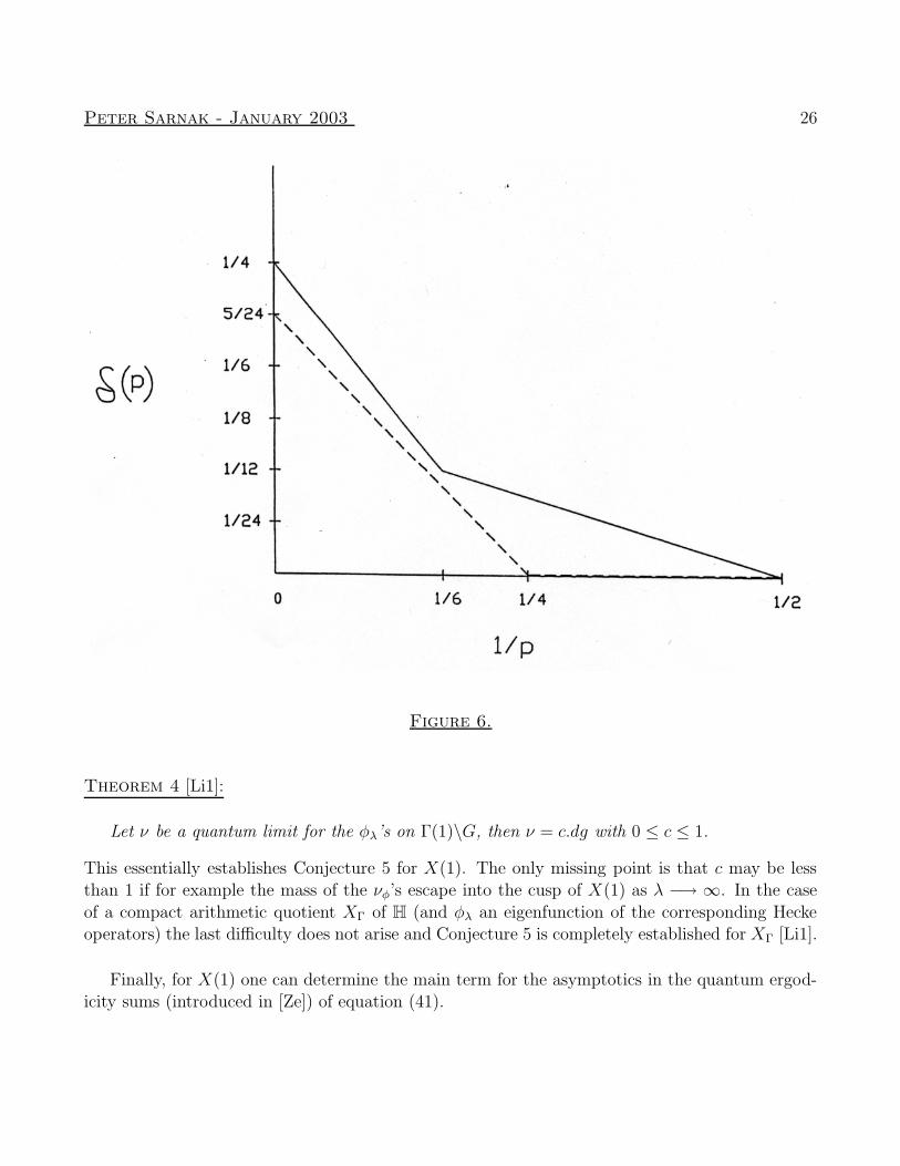
spectrum. Combining these sharp Lp bounds with (45) and interpolating yields subconvex boundsfor all 2 ≤ p ≤ ∞. In Figure 6 the exponent δ(p) of λ in these bounds is graphed against 1/p. The

solid lines corresponds to the convex bound (39) and the dashed lines to the subconvex bounds. Arandom wave model for the eigenfunctions of the quantization of a classically chaotic Hamiltonian

is put forth in [Be]. In [H-R] this is tested numerically for X(1) as far as the behavior of thevalue distribution of φλ(z) and E(z, 1

2+ it) as the energy goes to infinity. In particular they find

a Gaussian behavior. Thus we expect that the odd moments of φλ and E to go to zero and theeven moments (at least in the form (b)) to remain bounded. For special φλ’s (the dihedral ones)

on X(N) one can prove this uniform boundedness of the L4 norms. Moreover, (48) applied to thecase φ1 = φ2 = φ3 = φλ together with known sub-convexity bounds for degree 2 L-functions [Iw1]

show that the third moment

∫

X(1)

φ3λ dA, goes to zero as λ −→ ∞ [Wa].

10At present the proof of (a) which is involved uses Conjecture 2 and (32) freely. We expect in the end to getaround this.


Figure 6.

Theorem 4 [Li1]:

Let ν be a quantum limit for the φλ’s on Γ(1)\G, then ν = c.dg with 0 ≤ c ≤ 1.

This essentially establishes Conjecture 5 for X(1). The only missing point is that c may be lessthan 1 if for example the mass of the νφ’s escape into the cusp of X(1) as λ −→ ∞. In the case

of a compact arithmetic quotient XΓ of H (and φλ an eigenfunction of the corresponding Heckeoperators) the last difficulty does not arise and Conjecture 5 is completely established for XΓ [Li1].

Finally, for X(1) one can determine the main term for the asymptotics in the quantum ergod-icity sums (introduced in [Ze]) of equation (41).


Theorem 5 [L - S2]:

There is quadratic form B(f) on C∞0 (Γ(1)\H) such that

(a)∑

λj≤λ|µφj

(f) − f |2 = B(f)√λ + o

(√λ)

as λ −→ ∞.

(b) The polarization of B satisfies

B(f1,4f2) = B(4f1, f2)

(c) Defining the operator A by

〈Af1, f2〉 = B(f1, f2) .

A extends to a non-negative self-adjoint operator which commutes with 4 and is diagonalized

by the E(z, 12+ it) and φλ’s. Moreover, the eigenvalue of A corresponding to φλ is essentially

L(12, φλ), where L(s, φ) is the standard L-function associated with φ (Appendix 1).

Thus the form B provides a non-negative self-adjoint operator on a Hilbert space whose eigen-

values are special values of a family of L-functions! In particular, L( 12, φ) ≥ 0 a fact that was

known by other means, (see [L-R] for the most general such non-negativity result). Since it is

known that many of the values L( 12, φ) are non-zero it follows that for most f , B(f) > 0. In

particular, this shows that the decay rate for Conjecture 1 predicted by the Lindelof Hypothesis

in (49) is sharp (at least up to the exponent ε). In Appendix 5 we give a comparison of (a) withthe variation of f along the geodesic flow. The discrepancy between the classical and quantum

fluctuations is given by the arithmetic factor L(

12, φ)

!

We make some brief comments about the methods used to prove these recent results. Theorem

3 is approached by using Parseval’s identity to express ‖ φλ ‖44 as follows:

‖ φλ ‖44 =

∑

j

∣

∣〈φ2λ, φj〉

∣

∣

2+ similar term from continuous spectrum . (50)

Now apply (48) to the terms 〈φ2λ, φj〉 which converts the j sum to a sum of degree 8 L-functions.

The recent advances in the theory of families of L-functions (see [I-S2]) and especially the methodsfor averaging over such families using various trace formulae can be applied. However being of

degree 8, there are a number of new difficulties that need to be overcome. One useful technicaldevice that we mention and which is used, is the recent GL(3) Voronoi Summation Formula [M-S].

In any case, suffice it to say that the key techniques used to prove Theorems 3 and 5 are those

from the theory of L-functions.


The approach in [Li1] to Theorem 4 is very different. We know that ν is Gt invariant but thatthis is far from sufficient to identify ν. The idea is to try use that the φλ’s are also eigenfunctions

of the Hecke operators Tp. Rather than describe the case of X(1) consider a higher dimensionalcase which is conceptually simpler. Let Γ ≤ G×G be an irreducible lattice such as SL(2,Z[

√2])

embedded diagonally in G × G via γ −→ (γ, γ ′), γ′ being the Galois conjugate of γ. There is asimilar theory of Maass cusp forms φλ1,λ2

(z1, z2) on the Hilbert modular manifold X = Γ\H × H.

Such a form is an eigenfunction of 4zjwith eigenvalue λj, j = 1, 2. The Laplacian on X is

4z1 + 4z2. One can construct a micro-local lift νφ on Γ\G×G, of |φ(z1, z2)|2 dv(z1, z2), see [Li2].Being an eigenfunction of both 4z, and 4z2 (which commute) one can show that a quantum limit,

that is a weak limit of the νφ’s, is invariant under the two parameter Cartan action on Γ\G×G;

Γg −→ Γg

((

et1/2 00 e−t1/2

)

,

(

et2/2 00 e−t2/2

))

. (51)

Unlike the case of the geodesic flow Gt there are much fewer measures invariant under such two

(or higher parameter) actions. This is the so-called measure rigidity phenomenon that has seenmany advances recently[Ru], [Ka-Sp], [E-K]. The flow (51) does not fall into the setting of these

works and in [Li1] a substitute theory is developed. One point worth noting is that progress onthese measure rigidity questions has only been possible assuming that such an ergodic invariant

measure has positive entropy. As mentioned earlier for X(1) any quantum limit has been shownto have positive entropy.

It is interesting that the problems discussed in these notes can be approached by such differentpoints of view. Moreover, having recast the problem in different terms (for example the Hilbert

problem on page 11 as a sub-convexity problem for automorphic L-functions see [I-S2], or Conjec-ture 5 as a measure rigidity problem) one finds that solution demands a significant advance in the

corresponding theory. Thus both sides are enriched.

To end, we point the reader to books [Ve], [He2] and [Iw2] which treat the basic material

concerning hyperbolic surfaces, the trace formula and Eisenstein series. Also, the books [Lan1]and [Bor] give introductions to the approach via representation theory of SL(2,R) and [L-P], via

scattering theory for the corresponding wave equation. An earlier review article of some of thematerial discussed in the lectures can be found in [Sa4].


Appendices

These appendices are meant to give brief descriptions and definitions of various objects that

were mentioned in the text. Detailed treatments can be found in the references.

Appendix 1: L-Functions

The analytic continuation and functional equation for the Riemann Zeta Function was men-

tioned in (3) and (4). The key tool used there, that is Poisson Summation, can also be usedto analytically continue Dirichlet’s L functions L(s, χ) and their generalizations to number fields

Hecke’s L-functions, L(s, λ). A Dirichlet character χ is a function from Z into C which is periodicof (minimal) period q ≥ 1 and which satisfies χ(mn) = χ(m)χ(n), χ(1) = 1 and χ(m) = 0 if

(m, q) > 1. The corresponding L-function is defined to be

L(s, χ) =

∞∑

n=1

χ(n)n−s = Πp

(1 − χ(p)p−s)−1 . (1)

The completed L-function Λ(s, χ) is defined by:

Λ(s, χ) = π−(s+aχ)/2 Γ

(

s+ aχ2

)

L(s, χ), (2)

where aχ = 1−χ(−1)2

. Λ(s, χ) is entire (if χ 6= 1) and satisfies the functional equation [Da]

Λ(s, χ) =τ(χ)

ia(χ)q1/2q

12−s Λ(1 − s, χ) (3)

where τ(χ) is the Gauss sum. q is called the conductor of χ.

The Hecke L-functions are defined in a similar way [Hec1];

L(s, λ) =∑

A6=0

λ(A)N(A)−s = ΠP

(1 − λ(P )N(P )−s)−1 (4)

where λ is a suitable character on the ideals of a number field K, A ranges over the non-zerointegral ideals, P over the prime ideals and N(A) is the norm of A. For us an interesting example

is K = Q(√

2) = α = a + b√

2 |a, b ∈ Q. The ring of integers of K, OK is simply equal toa + b

√2 |a, b ∈ Z. The units in Ok are generated by ε0 = 1 +

√2. For α ∈ K let α′ denote


its Galois conjugate. OK happens to have class number one, that is every ideal is principal. For0 6= m ∈ Z set

λm(α) =∣

∣

∣

α

α′

∣

∣

∣

iπmlog ε0 (5)

Clearly, λm(εα) = λm(α) for any unit ε. So λ is a character on the ideals of OK. It is an example

of a “Grossencharakter” of Hecke in that the values assumed by λ as α varies are dense in thecircle. Maass [Mas] showed how these may be used to construct Maass forms. If

φm(z) =∑

A6=0

λm(A)y1/2Kitm (2πN(A)y) cos(2πN(A)x) (6)

with tm = πmlog ε0

, then φm satisfied (13) for γ ∈ Γ(4) and with eigenvalue λm = 14+t2m. In particular,

X(4) has this explicit subsequence of eigenvalues (no explicit eigenvalues are known or expected

for X(1)).

The Dirichlet L-functions are Euler products of degree 1 (over Q) while the Hecke L-functions

L(s, λ) are Euler products of degree 1 over K. Euler products of higher degree are constructedfrom modular forms, with modularity replacing Poisson Summation in the proof of the analytic

continuation. To illustrate this, let φ be a Maass-Hecke eigenform as described in (30) and (13),for X(1). That is, φ ∈ L2

cusp(X(1)) and

4φ +(

14

+ t2φ)

φ = 0

Tnφ = λφ(n)φ

(7)

(note we changed to a more convenient parameter tφ where λφ = 14+t2φ). The (standard) L-function

associated to φ is denoted by L(s, φ) and is defined for <(s) large by

L(s, φ) =∞∑

n=1

λφ(n)n−s = Πp

(1 − λφ(p)p−s + p−2s)−1 . (8)

The sum to product formula follows from a similar relation that is satisfied by the Tn’s [Hec2]. It

is convenient to introduce the roots α(1)φ (p) and α

(2)φ (p) which are determined by

α(1)φ (p)α

(2)φ (p) = 1, α

(1)φ (p) + α

(2)φ (p) = λφ(p) . (9)


Thus (8) is the degree 2 Euler product

L(s, φ) = Πp

[

(1 − α(1)φ (p) p−s) (1 − α

(2)φ p−s)

]−1

(10)

The modularity of φ(z) is equivalent to L(s, φ) extending to an entire function and satisfying the

functional equation

Λ(s, φ) := π−s Γ(

s+itφ2

)

Γ(

s−itφ2

)

L(s, φ)

= Λ(1 − s, φ)

(11)

(we have assumed here that φ is unramified at ∞ that is that φ is even with respect to the isometryof X(1), z −→ −z).

Thus these Maass forms give Euler products of degree 2 over Q. Note that L(s, φm) = L(s, λm)in (4) (5) and (6) above, that is, the degree 1 Euler product over the quadratic extension K of Q is

a degree 2 Euler product over Q and corresponds to a modular form. In general, any automorphicform π on GL2(AK) gives an Euler product of degree 2 over K which has an analytic continuation

and functional equation relating s to 1−s and π to its contragredient π ([Go-Ja]). More generally,if π is automorphic and cuspidal on GLn(AK) its standard L-function L(s, π) is of degree n and

is entire [Go-Ja]. In fact, one of the main interests in these automorphic cusp forms π is that it is

believed that all L-functions (for example Hasse-Weil L-functions, Artin L-functions . . .) can beexpressed as finite products and quotients of such standard L-functions.

Next we discuss the formation of tensor power L-functions from these π’s. For these much less

is known. We restrict to the φ’s in (7). Let φ1, . . . φ` be ` such Maass forms. Define the degree 2`

tensor power function, L(s, φ1 × φ2 × · · ·φ`) by

L(s, φ1 × φ2 × · · ·φ`) = ΠpLp(s, φ1 × φ2 · · · × φ`) (12)

where

Lp(s, φ1 × · · · × φ`) =∏

εj∈1,2

j=1,··· ,`

(

1 − α(ε1)φ1

(p)α(ε2)φ2

(p) · · · α(ε`)φ`

(p) p−s)−1

(13)


The completed L-function Λ(s, φ1×φ2 · · ·×φ`) is defined as usual by tacking on the correspondingproduct of 2` Gamma factors as in (11). It is believed that these Λ(s, φ1×φ2 · · ·×φ`) have analytic

continuations (except for possible poles at s = 0 and 1) and functional equations. This is knownto be valid for ` = 2 and 3. The case ` = 2 is known as the Rankin-Selberg L-function and its

value for s on the critical line (that is <(s) = 12) arose in (27) (though in (27) one of the forms

is holomorphic rather than a Maass form but the theory is the same). The analytic continuation

and functional equation for ` = 3 is due to [Ga] and [PS-R]. The special value at s = 12

of these

L-functions is at the heart of the identity (48).

If φ1 = φ2 = · · · = φ` one is led to form the symmetric tensor power L-functions. Define thedegree `+ 1, L-function L(s, φ, sym`), as follows:

L(s, φ, sym`) = ΠpLp(s, φ, sym`) (14)

where

Lp(s, φ, sym`) = Π`k=0 (1 − (α

(1)φ (p))j (α

(2)φ (p))`−j p−s)−1 . (15)

As before, one forms the corresponding completed function, Λ(s, φ, sym`). Again, it is conjectured

that these have analytic continuations and functional equations. The meromorphic continuationand functional equation is known for these for ` ≤ 9 [Sh]. The recent developments [K] and [K-S]

mentioned in Sections 1 and 2, establish that Λ(s, φ, sym`) is entire (except perhaps for poles ats = 0 and 1) for ` = 3 and 4 (the case ` = 2 is due to [Shi].) Moreover, they show in these

cases that there is an automorphic form π` on GL`+1(A ) whose L-function, L(s, π`) is equal toL(s, π, sym`). This correspondence (π, sym`) −→ π` is the sym` : GL(2) −→ GL(` + 1) functorial

lift. It is a special, but quite striking and useful instance of the general functoriality conjecture[La2].

It is the analytic properties of the L-functions such as their size on <(s) = 12

that is of most

use to us. In this connection the Grand Riemann Hypothesis GRH, is decisive. It asserts thatthe zeroes of any of the functions Λ(s, π) mentioned above (here we are thinking of π being an

automorphic form on GLn) are on the line <(s) = 12. A particular consequence of GRH is the

Grand Lindelof Hypothesis GLH, which asserts that for π of fixed degree n say and ε > 0

L

(

1

2+ it, π

)

ε,n

(C(π, t))ε , (16)

where C(π, t) is the “analytic conductor” defined in [I-S]. For example, for our Maass forms φ on


X(1) with eigenvalue λφ = 14+ t2φ, C(φ, 0) = λφ. For a Dirichlet L-function L(s, χ), C(χ, t) = (|t|+

1)(q+1) while for the L-functions L(s, φλ×φλ×φ) with φ fixed and λ −→ ∞, C(φλ×φλ×φ, 0) = λ2φ.

If the Ramanujan Conjectures (32) and their generalizations are true then for δ > 0, L(s, π)uniformly bounded for <(s) ≥ 1 + δ. This will not continue to hold even on <(s) = 1, however

the GLH asserts that it is almost true up to <(s) = 12. That is, all L-functions are bounded by an

arbitrary small power of their conductor in <(s) ≥ 12. It is this technical looking feature that is

very useful in the study of the eigenfunctions. In general, the only bound we have is the convexity

bound (see [Har])

L

(

1

2+ it, π

)

ε

[C(π, t)]14+ε . (17)

A number of the problems discussed in these notes are resolved by establishing subconvex estimates

for a suitable family of π’s. That is, a δ > 0 is produced so that

L

(

1

2, π

)

(C(π, 0))14−δ, (18)

for π in the family. See [F], [I-S2] for recent reviews.

Appendix 2: Frobenius Automorphisms

We review the definition of the Frobenius element. Details can be found in standard books

on algebraic number theory, for example [Lan2] and [C-F]. Let K be a finite Galois extension ofQ and G the corresponding Galois group. The ring of integers of K denoted OK, is a Dedekind

domain. Let p be a rational prime. The principal ideal (p) factors into a product of prime ideals(p) = (ß1ß2 . . . ßr)

e. The integer e is the ramification index of p and is equal to 1 for all primes

p not dividing the discriminant of K. We restrict attention to such unramified primes. If ß|pand σ ∈ G then σ(ß)|p and in fact G acts transitively on the primes ß dividing p. For such ß

the decomposition group Gß is the corresponding stabilizer of ß, that is σ ∈ G|σ(ß) = ß. Thedifferent decomposition groups for ß|p are conjugate in G. Now Gß acts in the obvious way as

automorphisms of the finite field OK/ß all of which fix the subfield Z/pZ. Denote the degree of

the field extension (OK/ß)/(Z/pZ) by f . Since we are assuming that e = 1, fr = deg(K/Q) = n.Also, since e = 1, Gß is isomorphic to Gal((OK/ß)/(Z/pZ)). By the theory of finite fields the

latter is cyclic of order f and is generated by the Frobenius automorphism x −→ xp. We callthe corresponding element of Gß, Frobß. It satisfies the relation Frobß(α) ≡ αp mod ß, for all

α ∈ OK. The different elements Frobß ∈ G for ß|p are conjugate in G. In this way we obtainfor each unramified prime p a conjugacy class Frobp in G. If p is ramified in K we can still


define Frobenuis elements Frobß in Gß but they are only determined up to the subgroup of inertia;ker : Gß −→ Gal((OK/ß)/(Z/pZ)).

Frobp tells us how (p) factors in OK. For example, if Frobp = 1 in G then (p) = ß1ß2 . . . ßnand OK/ßj ∼= Z/pZ, that is p splits completely. If K is the splitting field of f(x) ∈ Z[x] then inthis case f splits into linear factors over Z/pZ.

Using Brauer’s theorem on characters of finite groups [Br] together with class field theory

one can show (Artin) that the Artin L-function defined in (14) can be expressed as a ratio ofproducts of the Hecke L-functions L(s, λ), for suitable finite order characters λ on suitable field

extensions. In particular, this yields the meromorphicity and exact functional equation for L(s, ρ)after completing it with an appropriate archimedian factor. The possible archimedian factors in

this 2-dimensional case are (2π)−sΓ(s), (π−s/2Γ(s/2))2 or (π−(s+1)/2Γ( s+12

))2. In the first case ρ iscalled odd while in the second and third cases it is called even. The cases odd or even can be

characterized by whether det ρ(c) is −1 or 1 where c is a complex conjugation in Gal(Q/Q). Itis the even ρ which give rise to Maass forms with eigenvalue 1

4. The fully unramified archimedian

factor is the second case above and it corresponds to a cosine series in (15). The integer appearingin the functional equation of L(s, ρ) (in the same way as q appears in (3) of Appendix 1 for L(s, χ))

is called the conductor of ρ and it can be computed in terms of local ramification [C-F].

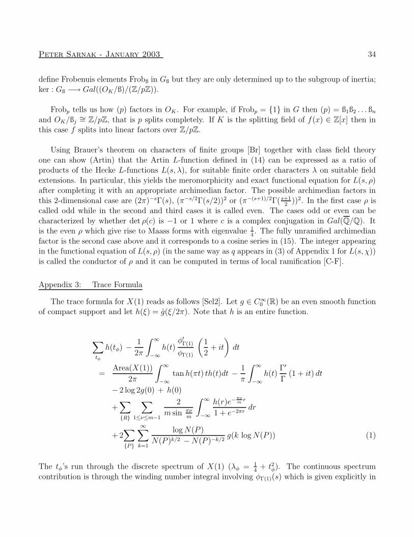
Appendix 3: Trace Formula

The trace formula for X(1) reads as follows [Sel2]. Let g ∈ C∞0 (R) be an even smooth function

of compact support and let h(ξ) = g(ξ/2π). Note that h is an entire function.

∑

tφ

h(tφ) − 1

2π

∫ ∞

−∞h(t)

φ′Γ(1)

φΓ(1)

(

1

2+ it

)

dt

=Area(X(1))

2π

∫ ∞

−∞tan h(πt) th(t)dt − 1

π

∫ ∞

−∞h(t)

Γ′

Γ(1 + it) dt

− 2 log 2g(0) + h(0)

+∑

R

∑

1≤ν≤m−1

2

m sin πνm

∫ ∞

−∞

h(r)e−πνmr

1 + e−2πrdr

+ 2∑

P

∞∑

k=1

logN(P )

N(P )k/2 −N(P )−k/2g(k logN(P )) (1)

The tφ’s run through the discrete spectrum of X(1) (λφ = 14

+ t2φ). The continuous spectrum

contribution is through the winding number integral involving φΓ(1)(s) which is given explicitly in


(24). The sum P is over primitive hyperbolic conjugacy classes of Γ(1). γ ∈ Γ is primitive ifγ 6= γν1 for any γ1 ∈ Γ and |ν| ≥ 2. γ is hyperbolic if |trace(γ)| > 2. A hyperbolic γ ∈ SL(2,R)

can be conjugated (in SL(2,R)) into the form ±(

(N(γ))1/2 00 N(γ)−1/2

)

with N(γ) > 1. γ fixes a

unique geodesic ` in H and ` modulo γ has length logN(γ). In this way the set P correspondsto the set of primitive closed geodesic on X(1). The sum R is over elliptic conjugacy classes of

which there are two, one of order m = 2 (in PSL(2,Z)) and the other of order m = 3.

The left-hand side of (1) is the spectral side of the trace formula being a sum over the discrete

and continuous spectrum. The right-hand side being over the closed geodesics is called the geomet-ric side (or the orbital integral side since in the derivation of the formula these terms arise as orbital

integrals). The geometric side which in the most general setting [A] can be very complicated isnevertheless quite explicit. For the case at hand, the lengths of the primitive closed geodesics are

precisely the numbers 2 log εd, where 0 < d ≡ 0 or 1 mod (4) is square-free and εd is the funda-

mental solution t0+√du0

2to the Pell equation t2 − du2 = 4, with multiplicity the class number h(d)

of integral binary quadratic forms of discriminant d. The fact that the geometric side is explicit is

at the heart of many modern applications of the general trace formula. One strategy being thatone computes explicitly the geometric sides for quotients Γ\G and Γ′\G′ of different (adele) groups

G and G′. In some special but striking cases one can match the corresponding geometric sides.This leads to correspondences between the spectral sides which then typically establishes a form

of a functorial correspondence [La4]. The cyclic base change theorem for GL2 mentioned in the

introduction is proved this way using a Galois twisted version of the trace formula.

Returning to the case of X(1), we apply (1) with hT (t) = H(

tT

)

for a fixed H and let T −→ ∞.For T large enough the contribution to the hyperbolic conjugacy classes is zero and hence for any

such H we have

∑

φ

H

(

tφT

)

− 1

2π

∫ ∞

−∞H

(

t

T

)

φ′Γ(1)

φΓ(1)

(

1

2+ it

)

dt

∼ Area(X(1))

2π

∫ ∞

−∞H

(

t

T

)

tan h(πt) tdt

By an approximation argument this leads to

∑

|tφ|≤T1 − 1

2π

∫ T

−T

φ′Γ(1)

φΓ(1)

(

1

2+ it

)

dt ∼ Area(X(1))

2πT 2 . (2)


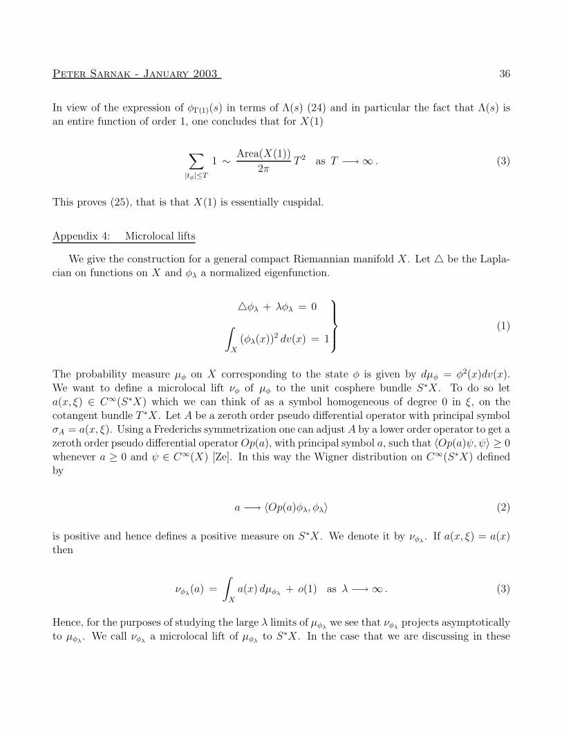
In view of the expression of φΓ(1)(s) in terms of Λ(s) (24) and in particular the fact that Λ(s) isan entire function of order 1, one concludes that for X(1)

∑

|tφ|≤T1 ∼ Area(X(1))

2πT 2 as T −→ ∞ . (3)

This proves (25), that is that X(1) is essentially cuspidal.

Appendix 4: Microlocal lifts

We give the construction for a general compact Riemannian manifold X. Let 4 be the Lapla-cian on functions on X and φλ a normalized eigenfunction.

4φλ + λφλ = 0

∫

X

(φλ(x))2 dv(x) = 1

(1)

The probability measure µφ on X corresponding to the state φ is given by dµφ = φ2(x)dv(x).

We want to define a microlocal lift νφ of µφ to the unit cosphere bundle S∗X. To do so let

a(x, ξ) ∈ C∞(S∗X) which we can think of as a symbol homogeneous of degree 0 in ξ, on thecotangent bundle T ∗X. Let A be a zeroth order pseudo differential operator with principal symbol

σA = a(x, ξ). Using a Frederichs symmetrization one can adjust A by a lower order operator to get azeroth order pseudo differential operatorOp(a), with principal symbol a, such that 〈Op(a)ψ, ψ〉 ≥ 0

whenever a ≥ 0 and ψ ∈ C∞(X) [Ze]. In this way the Wigner distribution on C∞(S∗X) definedby

a −→ 〈Op(a)φλ, φλ〉 (2)

is positive and hence defines a positive measure on S∗X. We denote it by νφλ. If a(x, ξ) = a(x)

then

νφλ(a) =

∫

X

a(x) dµφλ+ o(1) as λ −→ ∞ . (3)

Hence, for the purposes of studying the large λ limits of µφλwe see that νφλ

projects asymptotically

to µφλ. We call νφλ

a microlocal lift of µφλto S∗X. In the case that we are discussing in these


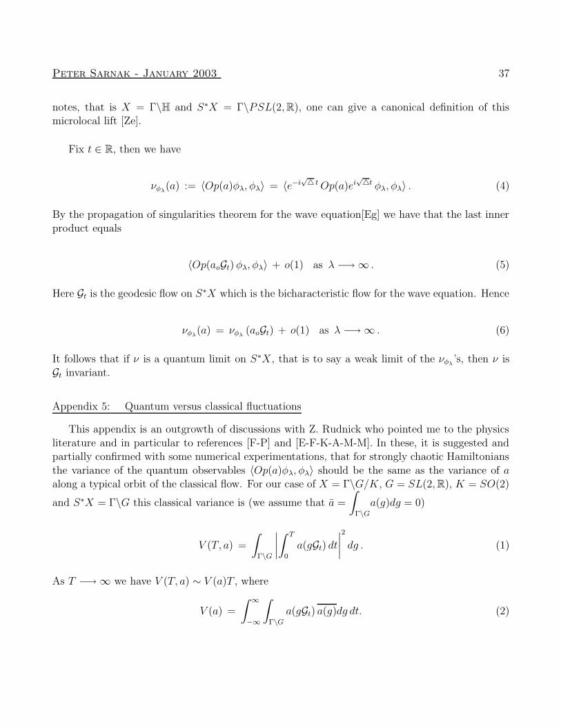
notes, that is X = Γ\H and S∗X = Γ\PSL(2,R), one can give a canonical definition of thismicrolocal lift [Ze].

Fix t ∈ R, then we have

νφλ(a) := 〈Op(a)φλ, φλ〉 = 〈e−i

√4 tOp(a)ei

√4t φλ, φλ〉 . (4)

By the propagation of singularities theorem for the wave equation[Eg] we have that the last inner

product equals

〈Op(aoGt)φλ, φλ〉 + o(1) as λ −→ ∞ . (5)

Here Gt is the geodesic flow on S∗X which is the bicharacteristic flow for the wave equation. Hence

νφλ(a) = νφλ

(aoGt) + o(1) as λ −→ ∞ . (6)

It follows that if ν is a quantum limit on S∗X, that is to say a weak limit of the νφλ’s, then ν is

Gt invariant.

Appendix 5: Quantum versus classical fluctuations

This appendix is an outgrowth of discussions with Z. Rudnick who pointed me to the physics

literature and in particular to references [F-P] and [E-F-K-A-M-M]. In these, it is suggested andpartially confirmed with some numerical experimentations, that for strongly chaotic Hamiltonians

the variance of the quantum observables 〈Op(a)φλ, φλ〉 should be the same as the variance of aalong a typical orbit of the classical flow. For our case of X = Γ\G/K, G = SL(2,R), K = SO(2)

and S∗X = Γ\G this classical variance is (we assume that a =

∫

Γ\Ga(g)dg = 0)

V (T, a) =

∫

Γ\G

∣

∣

∣

∣

∫ T

0

a(gGt) dt∣

∣

∣

∣

2

dg . (1)

As T −→ ∞ we have V (T, a) ∼ V (a)T , where

V (a) =

∫ ∞

−∞

∫

Γ\Ga(gGt) a(g)dg dt. (2)


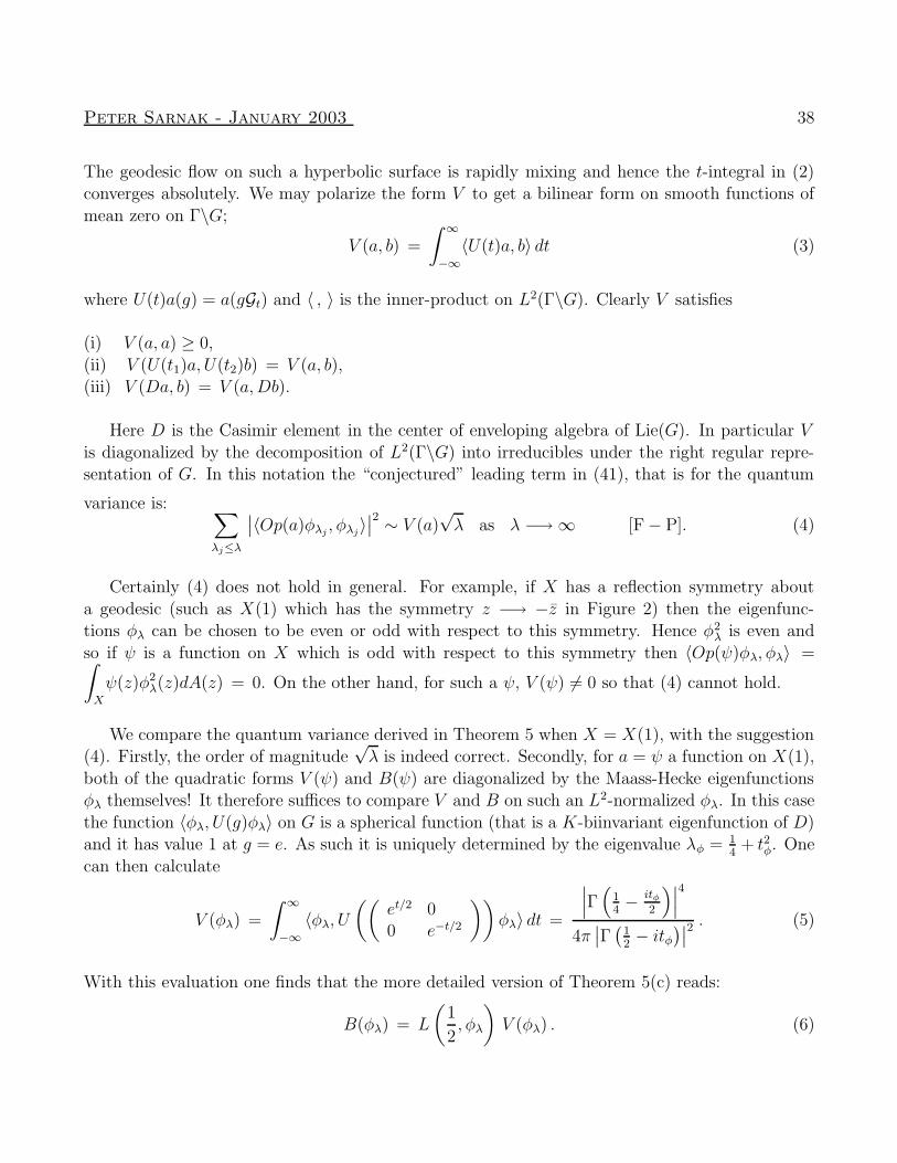
The geodesic flow on such a hyperbolic surface is rapidly mixing and hence the t-integral in (2)converges absolutely. We may polarize the form V to get a bilinear form on smooth functions of

mean zero on Γ\G;

V (a, b) =

∫ ∞

−∞〈U(t)a, b〉 dt (3)

where U(t)a(g) = a(gGt) and 〈 , 〉 is the inner-product on L2(Γ\G). Clearly V satisfies

(i) V (a, a) ≥ 0,

(ii) V (U(t1)a, U(t2)b) = V (a, b),(iii) V (Da, b) = V (a,Db).

Here D is the Casimir element in the center of enveloping algebra of Lie(G). In particular V

is diagonalized by the decomposition of L2(Γ\G) into irreducibles under the right regular repre-sentation of G. In this notation the “conjectured” leading term in (41), that is for the quantum

variance is:∑

λj≤λ

∣

∣〈Op(a)φλj, φλj

〉∣

∣

2 ∼ V (a)√λ as λ −→ ∞ [F − P]. (4)

Certainly (4) does not hold in general. For example, if X has a reflection symmetry about

a geodesic (such as X(1) which has the symmetry z −→ −z in Figure 2) then the eigenfunc-tions φλ can be chosen to be even or odd with respect to this symmetry. Hence φ2

λ is even and

so if ψ is a function on X which is odd with respect to this symmetry then 〈Op(ψ)φλ, φλ〉 =∫

X

ψ(z)φ2λ(z)dA(z) = 0. On the other hand, for such a ψ, V (ψ) 6= 0 so that (4) cannot hold.

We compare the quantum variance derived in Theorem 5 when X = X(1), with the suggestion(4). Firstly, the order of magnitude

√λ is indeed correct. Secondly, for a = ψ a function on X(1),

both of the quadratic forms V (ψ) and B(ψ) are diagonalized by the Maass-Hecke eigenfunctionsφλ themselves! It therefore suffices to compare V and B on such an L2-normalized φλ. In this case

the function 〈φλ, U(g)φλ〉 on G is a spherical function (that is a K-biinvariant eigenfunction of D)and it has value 1 at g = e. As such it is uniquely determined by the eigenvalue λφ = 1

4+ t2φ. One

can then calculate

V (φλ) =

∫ ∞

−∞〈φλ, U

((

et/2 00 e−t/2

))

φλ〉 dt =

∣

∣

∣Γ(

14− itφ

2

)∣

∣

∣

4

4π∣

∣Γ(

12− itφ

)∣

∣

2 . (5)

With this evaluation one finds that the more detailed version of Theorem 5(c) reads:

B(φλ) = L

(

1

2, φλ

)

V (φλ) . (6)


Thus by inserting the arithmetical factor L(

12, φ)

as a correction to the classical variance we obtainthe correct quantum variance! Note that if φ is odd with respect to the symmetry z −→ −z then

Λ(s, φ) is odd under s −→ 1 − s, so that L(

12, φ)

= 0 and hence B(φ) = 0, as it must be. Thepleasing relation (6) between the quantum and classical variances when X is arithmetic, suggest

that perhaps (4) is true for the generic hyperbolic surface in Teichmuller space. It would beinteresting to check this numerically.

The same physics papers above go on to conjecture that after normalization by the variancethe observables 〈Op(a)φλ, φλ〉 becomes Gaussian as λ −→ ∞ (the numerics for this are quite

convincing). For the classical motion such a central limit theorem is valid [Ra]. However, forX(1) such a Gaussian behavior for the quantum observables is unlikely to be true. At least such a

behavior would violate certain conjectures. Consider again the case that Op(a) is a multiplication

operator by a fixed even Hecke-Maass form φ on X(1), for which L(

12, φ)

6= 0 (which is expected tobe the case for all such φ). Then according to (48) the distribution question is essentially one about

the distribution of L(

12, sym2φλ × φ

)

as λ −→ ∞. Now the set of L-functions L(s, sym2φλ × φ),λj ≤ λ is a family of L-functions in the sense of [Ka-Sa]. It has a SO(even) symmetry (one

can check this by examining the 1-level density of low-lying zeros which follow WSO(even) density[Ka-Sa], at least for a restricted set of test functions). Now if we invoke the Conjectures [Ke-

Sn] concerning the moments of the special value at s = 12

for this family, then we conclude thatdistribution of L

(

12, sym2φλ × φ

)

cannot be Gaussian. The point is that L(

12, sym2φλ × φ

)

is

large too often rendering the moments to be infinite. On the other hand, by analogy with thedistribution of log

∣

∣ζ(

12

+ it)∣

∣ as t −→ ∞ [Sel3] and random matrix considerations [Ke-Sn] for this

family one might expect that for X(1)

log(

|〈φ2λ, φ〉|λ1/4

)

(log logλ)1/2

becomes Gaussian about a drifting mean as λ −→ ∞.

Appendix 6: Cancellation in shifted sums

We describe the connection between the sums (21) and the spectrum of X(N). For definiteness

we consider the congruence surfacesX0(N) = Γ0(N)\H where Γ0(N) =

γ =

(

a bc d

)

∈ Γ(1) : N |c

.

For this group the subgroup stabilizing ∞ is Γ∞ =

±(

1 m0 1

)

|m ∈ Z

. Let f be a fixed holo-

morphic cusp form of even integral weight k for Γ0(N). The definition of such forms being as in(26) except that the weight 4 is allowed to be any positive even integer k and Γ(N) is replaced by


Γ0(N). We may expand f in a Fourier series

f(z) =

∞∑

n=1

af (n)e(nz) . (1)

Letλf(n) := af(n)n(1−k)/2 . (2)

With this normalization the classical Ramanujan Conjecture (which is equivalent to the bound

(33) for the Hecke operators in this setting) which was proved in [De], asserts that for any ε > 0

λf(n) = Oε(nε) . (3)

Fix ν1, ν2, h positive integers and set

Df (s, ν1, ν2, h) =∑

ν1m−ν2n=h

λf (m)λf(n)

( √mnν1ν2

mν1 + nν2

)k−1

(mν1 + nν2)−s (4)

In view of (3) this converges absolutely for <(s) > 1. In order to investigate the analytic propertiesof D(s) define the Poincare series Uh(z, s) as follows

Uh(z, s) =∑

γ∈Γ∞\Γ0(ν1ν2N)

y(γz)s e(−hx(γz)) . (5)

The series (5) converges absolutely for <(s) > 1 and since yse(−hx) is invariant under Γ∞ itfollows that Uh(γz, s) = Uh(z, s) for γ ∈ Γ0(Nν1ν2). Moreover, a direct calculation shows that

4 (yse(−hx)) + s(1 − s) (yse(−hx)) = −4π2h2ys+2 e(−hx) . (6)

Hence

4Uh(z, s) + s(1 − s)Uh(z, s) = −4π2h2Uh(z, s + 2) . (7)

Inverting this relation using the resolvent gives

Uh(z, s) = (4 + s(1 − s))−1 Uh(z, s+ 2) (8)

(There is a technical issue that Uh(·, s) is not in L2(X0(Nν1ν2)) but this difficulty can easily be

overcome in what follows). From (8) we see that since the series Uh(z, s + 2) is holomorphic in<(s) > 0, Uh(z, s) is meromorphic in <(s) > 1

2with possible poles at s(1 − s) = λφ where λφ

is an eigenvalue of 4 on X0(ν1ν2N). For <(s) > 12

only eigenvalues λφ <14

are relevant. Theeigenvalue λφ = 0 does not contribute a pole since 〈Uh(z, s), 1)〉 = 0 (at least formally). Thus

the main conjecture about the low energy spectrum, that is Conjecture 2 implies that Uh(z, s) is

analytic in <(s) > 12. Theorem 2 ensures that in any case Uh(z, s) is analytic in <(s) > 39

64.


To connect this with Df(s) let V (z) = f(ν1z)f(ν2z)yk. V is Γ0(Nν1ν2) invariant and is rapidly

decreasing as z approaches the cusps of X0(ν1ν2N). Consider

I = 〈Uh, V 〉 =

∫

X0(Nν1ν2)

Uh(z, s)V (z)dA(z) . (9)

Unfolding this integral according to the definition of Uh and the invariance of V yields

I =

∫ ∞

0

∫ 1

0

V (z)ys e(−hx) dxdyy2

. (10)

Now do the x-integral first and use (1) and then do the y-integral to get

I = (2π)−(s+k−1) Γ(s+ k − 1) (ν1ν2)1−k2 Df (s, ν1, ν2, h) . (11)

That is

Df(s, ν1, ν2, h) =(2π)s+k−1 (ν1ν2)

k−12

Γ(s+ k − 1)〈Uh(·, s), V 〉 . (12)

From this and the previous discussion we may deduce that Df(s) is meromorphic in <(s) > 12

and

if Conjecture 2 is true that Df(s) is analytic in <(s) > 12. With quite a bit more effort [Sa5] one

can establish polynomial bounds for the growth of Df(s) in <(s) > 12

when |=(s)| −→ ∞. With

this one can use Mellin inversion and standard contour shifts to deduce the cancellations claimedin (21), see [Sa5].

Appendix 7: Numerical Methods

The first attempts at the numerical computation of the spectrum of X(1) were carried out in[C]. Their method yields the first few odd eigenfunctions but it was not successful in picking up the

elusive even eigenfunctions. There followed computations by others and in one such computationthe zeros of the Riemann Zeta Function appeared among the number 1

2+ itφ (where as usual

λφ = 14

+ t2φ)! Eventually the reason for this was discovered in [He2]. The numerical methodwas faulty in that it allowed the eigenfunctions to have logarithmic singularities. These fake

eigenfunctions were the ones that gave rise to eigenvalues which correspond to the zeros of ζ(s).

The method developed in [He1] to compute the spectrum is known as “collocation.” The

eigenfunctions φ (cusp forms) in question have Fourier developments as in (18)

φ+(z) =

∞∑

n=1

ρφ(n)y1/2Kitφ(2πny) cos(2πnx) ,

φ−(z) =

∞∑

n=1

ρφ(n)y1/2Kitφ (2πny) sin(2πnx) .

(1)


Here φ+(z) is even and φ−(z) is odd. The numbers tφ and ρφ(n) are what we want to compute.Note that the Bessel function Kitφ(y) is exponentially decreasing for y |tφ|, so that the series

(1) is approximated to an accuracy of O(e−2πM) for y ≥√

32

, when truncating the series at n ≤M

(here we are thinking of tφ being of moderate size). What is lacking to ensure that φ(z) is a cuspform is the relation φ(−1/z) = φ(z).

The first method which is good to get eigenvalues of X(1) with λφ ≤ 250000 is as follows.Truncate (1) at n ≤ M and choose points z1, . . . , zM ∈ H which are evenly distributed in F(1).

The equations for the truncated series φ(M)(z);

φ(M)(zj) = φM)(−1/zj) (2)

yield a homogeneous linear system of M equations with M unknowns. They are of the form

M∑

n=1

ρ(n) In(zj, t) = 0 (3)

whereIn(z, t) =

√y∗Kit(2πny

∗) cos(2πnx∗) −√y Kit(2πny) cos(2πnx) (4)

and z∗ = −1/z.

One way to proceed at this point is to seek solutions t ≤ T of

det(In(zj, t))n = 1, . . .Mj = 1, . . .M

= 0 . (5)

However, it is more expedient to choose a second set of points w2, . . . , wM and to solve the linear

equations (by ellimination and setting ρ(1) = 1)

−I1(zj, t) =

M∑

n=2

ρ(z)(n) In(zj, t)

−I1(wj, t) =M∑

n=2

ρ(w)(n)In(wj, t)

(6)

for j = 2, . . .M .

For a genuine eigenvalue t = tφ we will have

ρ(z)(n) = ρ(w)(n), n = 2, . . .M . (7)


So one determines the t’s for which (7) is valid (actually one minimizes a related functional). Thisworks well for T ≈ 500. For larger T the system of linear equations becomes ill conditioned.

In order to deal with larger values of t, a somewhat different approach (inspired by [Sta]) istaken. The series (1) is truncated at say M ≈ 5T (with t ≈ T ) and yields a good approximation

of φ for z ∈ F(1). On other hand, for y small

ρ(n)y1/2Kit(2πny) =

∫ 1

0

φ+(x+ iy) cos(2πnx) dx . (8)

Replacing the integral by a sum (with Q large), we have

ρ(n)y1/2 Kit(2πny) ∼=1

Q

Q∑

j=1

φ+

(

j

Q+ iy

)

cos

(

2πn

Q

)

. (9)

By transforming the points jQ

+ iy into F(1) we can evaluate the right hand side of (9) with our Mterm truncation. This yields (for a given y) a system of linear equations for ρ(n), n ≤M (and once

these are determined many more coefficients can be computed from (8)). Proceeding as beforewith this linear system, set ρ(1) = 1 and solve for the coefficients with y and y ′. Then choose the

t’s so as to minimize |ρ(y)(n)− ρ(y′)(n)|. These linear equations turn out to be well conditioned forT as large as 11000 [He3]. To carry this out one also needs a fast routine to compute Kit(y) with

t large.

An excellent test as to whether the tφ’s and ρφ(n)’s are accurate is that if the spectrum is

simple then the coefficients must inherit the relations satisfied by the Hecke operators (30). That

is ρφ(n)ρφ(m) =∑

d|(n,m)

ρφ

(nm

d2

)

must hold. Since these relations were not imposed, their truth is

convincing evidence that genuine cusp forms are being picked up. By examining average deviationsin the Weyl count |j|λj ≤ λ| (see [St] for example) one can be convinced that no tφ’s were omitted

in the above calculations. The approach described above works equally well for computing thespectra of nonarithmetic triangle groups [He2].

The method used in [G-S] to obtain the plots in Figure 3 is quite different. They use thetrace formula in Appendix 3 together with the explicit knowledge of the length spectrum for X(1).

While this method only gives the first few eigenvalues it can be applied quite easily to X(N) with(N moderate) as well.

Acknowledgements:

I thank E. Lindenstrauss, Y. Petridis, J.P. Serre, F. Spinu and A. Strombergsson for their

comments on a preliminary version of this paper. Also, thanks to G. Pecht for her excellent jobin typing the manuscript.


References

[A] J. Arthur, In “Number Theory, Trace Formulas and Discrete Groups,” AcademicPress (1988), 11-29.

[Ar] E. Artin, Abh. Math. Sem., Hamburg (1924), 170-175.

[Be] L. Bers, ICM Proceedings (Edin. 1958), 349-361.

[Ber] M. Berry, J. Phys. A10 (1977), 2083-2091.

[Bo] E. Bombieri, Lectures on the zeta function (Italy, 2002).

[Bor] A. Borel, Camb. Tracts in Math., 130, (1977).

[Boo] A. Booker, “Poles of Artin L-functions and the strong Artin Conjecture,”preprint (2002).

[B-D-S-T] K. Buzzard, M. Dickinson, N. Shepherd-Barron and R. Taylor, D.M.J., Vol. 109(2001), 283-317.

[B-S] E. Bogomolny and C. Schmit, “Nonlinearity,” 6 (1993), 523-547.

[Br] R. Brauer, Annals of Math., Vol. 48, 2 (1947), 502-551.

[B-L] J. Bourgain and E. Lindenstrauss, “Entropy of quantum limits,” (to appear),CMP.

[Ca] P. Cartier, In computers in Number Theory (1969), 37-48, ed Atkin-Birch.

[C-F] J. Cassels and A. Frohlich, “Algebraic Number Theory,” A.P. (1967).

[Cl] L. Clozel, “Spectral theory of automorphic forms,” Lectures, Park City (2002).

[Co-PS-S] J. Cogdell, I. Piatetsky-Shapiro and P. Sarnak, “Estimates for Hilbert modularL-functions and applications,” (in preparation).

[Co] Y. Colin de Verdiere, Comm. Math. Phys. , 102 (1985), 497-502.

[Co2] Y. Colin de Verdiere, Ann Inst. Fourier, 32, (1983), 275-286 and 33, (1983),87-113.

[Da] H. Davenport, G.T.M., Vol. 74, Springer (1980).

[De] P. Deligne, Lecture Notes in Math., Vol. 179, Springer (1971), 139-172.

[D-I] J. Deshoulliers and H. Iwaniec, Comtemp. Math., 53 (1986), 51-97.

[D-F-I] W. Duke, J. Friedlander and H. Iwaniec, Annals of Math., 141 (1995), 423-441.

[D-SP] W. Duke and R. Schulze-Pillot, Invent. Math., 90 (1990), 49-57.

[Du-Iw] W. Duke and H. Iwaniec, Amer. Jnl. Math., 116 (1994), 207-217.


[Du-Gu] H. Duistermaat and V. Guillemin, Invent. Math., 29 (1975), 39-79.

[E-F-K-A-M-M] B. Eckhardt, S. Fishman, J. Keating, O. Agam, J. Main, K. Muller, Phys. Rev.E, Vol. 52, No. 6, (1995), 5893-5903.

[Eg] Y. Egorov, Uspehi. Mat. Nauk, 24 (1969), 5 (149), 235-236.

[E-K] M. Einsiedler and A. Katok, “Invariant measures on G/Γ for split simple LieGroups G”, preprint (2002).

[F] J. Friedlander, Proc. ICM, (Zurich 1994), 363-373.

[F-P] M. Feingold and A. Peres, Phys. Rev. A, Vol. 34, No. 1, (1986), 591-595.

[Ga] P. Garrett, Annals of Math., 125 (1987), 209-235.

[Ge] S. Gelbart, Ann. Math. Studies, 83 (1975).

[Ge-Ja] S. Gelbart and H. Jacquet, Ann. Sci. Ecole Norm. Sup., 11 (1978), 471-552.

[Go-Ja] R. Godement and H. Jacquet, L.N.M., 260, Springer (1972).

[G-S] V. Golovshanski and N. Smotrov, preprint Inst. App. Math. Khabarovsk (1982).

[Har] G. Harcos, IMRN (2002), 18, 923-932.

[Ha] H. Hasse, J. reine angew Math., 153 (1924) 113-130.

[Hec1] E. Hecke, Math. Zeit, Vol. 1 (1918), 357-376.

[Hec2] E. Hecke, Math. Ann., Vol. 114 (1937), 1-28.

[He1] D. Hejhal, Memiors of the AMS, 469 (1992).

[He2] D. Hejhal, S.L. Notes, Vol. 548 (1976) and Vol. 1001 (1980).

[He3] D. Hejhal in “Emerging Applications of Number Theory,” IMA Series 109,Springer, (1999), 291-315.

[H-R] D. Hejhal and Rackner, Exp. Math., 1 (1992), 275-305.

[Hel] R. Heller, Phys. Lett. Review, 53 (1984), 1515-1518.

[Hu] M. Huxley, in Banach Center Publ., 17 (1982), 217-306.

[Iw1] H. Iwaniec, J. reine angew Math., 428 (1992), 139-159.

[Iw2] H. Iwaniec, “Introduction to the spectral theory of automorphic forms,” RevistaMat. Iber. (1995).

[I-S1] H. Iwaniec and P. Sarnak, Annals of Math., 141 (1995), 301-320.

[I-S2] H. Iwaniec and P. Sarnak, GAFA (2000), 705-741.


[Ja-Sh] H. Jacquet and J. Shalika, Amer. Jnl. Math., 103 (1981), 499-558.

[Ju] C. Judge, JAMS 8 (1995), 715-759.

[Ja] D. Jakobson, Ann de l’Inst. Fourier, 44 (1994), 1477-1504.

[Ka-Sa] N. Katz and P. Sarnak, BAMS, Vol. 36, 1, (1999), 1-26.

[Ke-Sn] J. Keating and N. Snaith, CMP, 214, No. 1, (2000), 91-111.

[K] H. Kim, “Functoriality of the exterior square of GL4 and the symmetric fourthpower of GL2,” JAMS, Vol. 16, 1, (2002), 139-183.

[Kne] M. Kneser, “Quadratische formen,” Lecture Notes, Gottiugen (1974).

[K-S] H. Kim and F. Shahidi, Annals of Math., 155 (2002), 837-893.

[Kl] F. Klein, “Lectures on the Icosahedron,” Paul French Frubner Co. (1913).

[H-K] M. Harris and S. Kudla, Ann. of Math., 133 (1991), 605-672.

[Ku] N. Kuznietzov, Mat. SB. (NS) , 39 (1981), 299-342.

[Ki-Sa] H. Kim and P. Sarnak, Appendix to [K] (to appear), JAMS (2003).

[Ka-Sp] A. Katok and R. Spatzier, Erg. and Dyn. Systems, 16 (1996), 751-778.

[Lan1] S. Lang, “SL2(R),” Addison-Wesley (1975).

[Lan2] S. Lang, “Algebraic Number Theory,” Adison Wesley (1970).

[Lax] P. Lax, J. Evol. Equ., 1 (2001), 311-323.

[Laz] V.F. Lazutkin, “KAM Theory and Semi Classical Approximation to Eigenfunc-tions,” Ergeb. Math., Vol. 24, (1993).

[Li1] E. Lindenstrauss, “A proof of the quantum unique ergodicity conjecture,” (inpreparation).

[Li2] E. Lindenstrauss, IMRN, 17 (2001), 913-933.

[L-R] E. Lapid and S. Rallis, Annals of Math., 157 (2003), 1-26.

[L-R-S] W. Luo, Z. Rudnick and P. Sarnak, GAFA, 5 (1995), 387-401.

[L-P] P. Lax and R. Phillips, Annals of Math. Studies, Vol. 87, (1976).

[Lu] W. Luo, Annals of Math., 154 (2001), 477-502.

[La1] R. Langlands, Annals of Math. Studies, 96 (1980).

[La2] R. Langlands, S.L. Notes, Vol. 170 (1970), 18-61.

[La3] R. Langlands, S.L. Notes, Vol 544 (1976).


[La4] R. Langlands, In “Number Theory, Trace Formulas and Discrete Groups,” Aca-demic Press (1988), 125-257.

[L-P-S] A. Lubotzky, R. Phillips and P. Sarnak, Combinatorica, Vol 8, 3 (1988), 261-277.

[L-S1] W. Luo and P. Sarnak, Proc. Publ. IHES, 81 (1995), 207-237.

[L-S2] W. Luo and P. Sarnak, “Quantum ergodicity of eigenfunctions on SL2(Z)\H II”(in preparation).

[Mc] H. Mckean, J.D.G., 4 (1970) 359-366.

[Mi] S.D. Miller, J. reine agnew. Math., 533 (2001), 127-169.

[Mu] W. Muller, (2002), (in preparation).

[M-S] S.D. Miller and W. Schmid, “Automorphic Distributions, L-functions andVoronoi Summation for GL(3),” (2002), preprint.

[M] G. Margulis, J. Prob. Inf. Transmission, 24 (1988), 39-46.

[Mas] H. Maass, Math. Ann., 121 (1949), 141-183.

[Me] M. Mehta, “Random Matrices,” Acamedic Press, (1980).

[Mc-Si] H. Mckean and I. Singer, Jnl. of Diff. Geom., 1 (1967), 43-69.

[P-S1] R. Phillips and P. Sarnak, Invent. Math., 80 (1985), 339-364.

[P-S2] R. Phillips and P. Sarnak, Comm. Pure and Appl. Math, 38 (1985), 853-866.

[P-S3] R. Phillips and P. Sarnak, JAMS 5(2), No 1 (1992), 1-32.

[Pe] Y. Petridis, J. Funct. Anal., 124 (1944), 1, 61-94.

[PS-R] I. Piatetsky-Shapiro and S. Rallis, Compositio Math., 64 (1987), 31-115.

[Ra] M. Ratner, Israel Jnl. of Math., Vol. 16, (1973), 181-197.

[R-S] Z. Rudnick and P. Sarnak, CMP, 161 (1994), 195-213.

[Ru] D. Rudolph, Erg. th. and Dyn. Systems, 10 (1990), 395-406.

[Sa1] P. Sarnak, In “A panorama of number theory,” ed. Wustholz Cambridge(2002),121-127.

[Sa2] P. Sarnak, AMS Contemp. Math., 53 (1986).

[Sa3] P. Sarnak, Letter to Z. Rudnick, August, 2002.

[Sa4] P. Sarnak, “Arithmetic Quantum Chaos,” Israel Math. Conf. Proc., Vol. 8,Ramat Gan (1995), 183-236.

[Sa5] P. Sarnak, J. Funct. Anal., 184 (2001), 419-453.


[Sa-Wa] P. Sarnak and T. Watson, (in preparation).

[Sel3] A. Selberg, Collected Works, Springer, (1988), 341-355.

[Se] J. P. Serre, In “Algebraic Number Fields,” ed. Frohlich, Academic Press, (1977),193-268.

[Sel1] A. Selberg, Collected Works (Springer) (1989), 626-674.

[Sel2] A. Selberg, Proc. Symp. Pure Math., VIII (1965), 1-15.

[Si] B. Simon, Ann. of Math., 97 (1973), 247-274.

[So] C. Sogge, J. Func. Anal., 77 (1988), 123-138.

[Sta] H. Stark, in “Modular Forms,” Ellis Howard, (1984), editor R.Rankin, 263-268.

[St] G. Steil, Diplom. Math. Univ. Hamburg (1992).

[Ste] E. Stein, In “Lectures in Harmonic Analysis,” Princeton University Press (1986),307-356.

[Shi] G. Shimura, Proc. London Math. Soc., 31 (1975), 79-98.

[Shn] A. Shnirelman, Uspenski Math. Nauk, 29/6 (1974), 181-182.

[Sh] F. Shahidi, “Perspectives in Math.,” Vol. 10, A.P. (1990), 415-437.

[SP] R. Schulze-Pillot, D.M.J., 102 (2000), 351-357.

[Sp] F. Spinu, Thesis, Princeton University (2003).

[Str] A. Strombergsson (2003).

[Ta] K. Takeuchi, Math. Soc. Japan 29, 4 (1975), 600-662.

[Tu] J. Tunnel, B.A.M.S., 5 (1981), 173-175.

[To] A. Toth, IMRN, (2000), No. 14, 719-739.

[Ve] A. Venkov, Proc. of the Steklov Inst. of Math., Vol. 153, (1981), (AMS transla-tions Issue 4, (1982)).

[Wa] T. Watson, Thesis, Princeton University, (2002).

[Wol1] S. Wolpert, Invent. Math., Vol. 108, (1992), 67-89, 91-129.

[Wol2] S. Wolpert, Annals of Math., 139 (1994), 239-291.

[W] M. Wolf, J.D.G., 33 (1991), 487-539.

[Wei] A. Weil, Springer Lect. Notes, Vol 189 (1971).

[Ze] S. Zelditch, Duke Math. Jnl., 55 (1987), 919-941.

February 25, 2003

Spectra of Hyperbolic Surfaces - Mathweb.math.princeton.edu/sarnak/baltimore.pdf · Spectra of...

Documents

Transcript of Spectra of Hyperbolic Surfaces - Mathweb.math.princeton.edu/sarnak/baltimore.pdf · Spectra of...