HAL Id: hal-01402045https://hal.inria.fr/hal-01402045

Submitted on 24 Nov 2016

HAL is a multi-disciplinary open accessarchive for the deposit and dissemination of sci-entific research documents, whether they are pub-lished or not. The documents may come fromteaching and research institutions in France orabroad, or from public or private research centers.

L’archive ouverte pluridisciplinaire HAL, estdestinée au dépôt et à la diffusion de documentsscientifiques de niveau recherche, publiés ou non,émanant des établissements d’enseignement et derecherche français ou étrangers, des laboratoirespublics ou privés.

Distributed under a Creative Commons Attribution| 4.0 International License

Specifying and Verifying Properties of SpaceVincenzo Ciancia, Diego Latella, Michele Loreti, Mieke Massink

To cite this version:Vincenzo Ciancia, Diego Latella, Michele Loreti, Mieke Massink. Specifying and Verifying Propertiesof Space. 8th IFIP International Conference on Theoretical Computer Science (TCS), Sep 2014, Rome,Italy. pp.222-235, �10.1007/978-3-662-44602-7_18�. �hal-01402045�

Specifying and Verifying Properties of Space?

Vincenzo Ciancia1, Diego Latella1, Michele Loreti2, and Mieke Massink1

1 Istituto di Scienza e Tecnologie dell’Informazione ‘A. Faedo’, CNR, Italy2 Universita di Firenze, Italy

Abstract. The interplay between process behaviour and spatial aspectsof computation has become more and more relevant in Computer Sci-ence, especially in the field of collective adaptive systems, but also, moregenerally, when dealing with systems distributed in physical space. Tra-ditional verification techniques are well suited to analyse the temporalevolution of programs; properties of space are typically not explicitlytaken into account. We propose a methodology to verify properties de-pending upon physical space. We define an appropriate logic, stemmingfrom the tradition of topological interpretations of modal logics, datingback to earlier logicians such as Tarski, where modalities describe neigh-bourhood. We lift the topological definitions to a more general setting,also encompassing discrete, graph-based structures. We further extendthe framework with a spatial until operator, and define an efficient modelchecking procedure, implemented in a proof-of-concept tool.

1 Introduction

Much attention has been devoted in Computer Science to formal verifica-tion of process behaviour. Several techniques, such as run-time monitoringand model-checking, are based on a formal understanding of system re-quirements through modal logics. Such logics typically have a temporalflavour, describing the flow of events along time, and are interpreted invarious kinds of transition structures.

Recently, aspects of computation related to the distribution of systemsin physical space have become more relevant. An example is provided byso called collective adaptive systems3, typically composed of a large num-ber of interacting objects. Their global behaviour critically depends oninteractions which are often local in nature. Locality immediately posesissues of spatial distribution of objects. Abstraction from spatial distribu-tion may sometimes provide insights in the system behaviour, but this isnot always the case. For example, consider a bike (or car) sharing system

? Research partially funded by EU ASCENS (nr. 257414), EU QUANTICOL (nr.600708), IT MIUR CINA and PAR FAS 2007-2013 Regione Toscana TRACE-IT.

3 See e.g. the web site of the QUANTICOL project: http://www.quanticol.eu

having several parking stations, and featuring twice as many parking slotsas there are vehicles in the system. Ignoring the spatial dimension, on av-erage, the probability to find completely full or empty parking stationsat an arbitrary station is very low; however, this kind of analysis maybe misleading, as in practice some stations are much more popular thanothers, often depending on nearby points of interest. This leads to quitedifferent probabilities to find stations completely full or empty, depend-ing on the spatial properties of the examined location. In such situations,it is important to be able to predicate over spatial aspects, and eventu-ally find methods to certify that a given formal model of space satisfiesspecific requirements in this respect. In Logics, there is quite an amountof literature focused on so called spatial logics, that is, a spatial inter-pretation of modal logics. Dating back to early logicians such as Tarski,modalities may be interpreted using the concept of neighbourhood in atopological space. The field of spatial logics is well developed in termsof descriptive languages and computability/complexity aspects. However,the frontier of current research does not yet address verification problems,and in particular, discrete models are still a relatively unexplored field.

In this paper, we extend the topological semantics of modal logics toclosure spaces. As we shall discuss in the paper, this choice is motivatedby the need to use non-idempotent closure operators. A closure space(also called Cech closure space or preclosure space in the literature), isa generalisation of a standard topological space, where idempotence ofclosure is not required. By this, graphs and topological spaces are treateduniformly, letting the topological and graph-theoretical notions of neigh-bourhood coincide. We also provide a spatial interpretation of the untiloperator, which is fundamental in the classical temporal setting, arrivingat the definition of a logic which is able to describe unbounded areas ofspace. Intuitively, the spatial until operator describes a situation in whichit is not possible to “escape” an area of points satisfying a certain prop-erty, unless by passing through at least one point that satisfies anothergiven formula. To formalise this intuition, we provide a characterisingtheorem that relates infinite paths in a closure space and until formulas.We introduce a model-checking procedure that is linear in the size of theconsidered space. A prototype implementation of a spatial model-checkerhas been made available; the tool is able to interpret spatial logics on digi-tal images, providing graphical understanding of the meaning of formulas,and an immediate form of counterexample visualisation.4

4 Due to lack of space all the proofs are omitted and can be found in [10].

Related work. We use the terminology spatial logics in the “topological”sense; the reader should be warned that in Computer Science literature,spatial logics typically describe situations in which modal operators areinterpreted syntactically, against the structure of agents in a process cal-culus (see [8,6] for some classical examples). The object of discussion inthis research line are operators that quantify e.g., over the parallel sub-components of a system, or the hidden resources of an agent. Furthermore,logics for graphs have been studied in the context of databases and pro-cess calculi (see [7,15], and references), even though the relationship withphysical space is often not made explicit, if considered at all. The influ-ence of space on agents interaction is also considered in the literature onprocess calculi using named locations [11].

Variants of spatial logics have also been proposed for the symbolic rep-resentation of the contents of images, and, combined with temporal logics,for sequences of images [12]. The approach is based on a discretisation ofthe space of the images in rectangular regions and the orthogonal projec-tion of objects and regions onto Cartesian coordinate axes such that theirpossible intersections can be analysed from different perspectives. It in-volves two spatial until operators defined on such projections consideringspatial shifts of regions along the positive, respectively negative, directionof the coordinate axes and it is very different from the topological spatiallogic approach.

A successful attempt to bring topology and digital imaging together isrepresented by the field of digital topology [22,25]. In spite of its name, thisarea studies digital images using models inspired by topological spaces,but neither generalising nor specialising these structures. Rather recently,closure spaces have been proposed as an alternative foundation of digi-tal imaging by various authors, especially Smyth and Webster [23] andGalton [17]; we continue that research line, enhancing it with a logical per-spective. Kovalevsky [19] studied alternative axioms for topological spacesin order to recover well-behaved notions of neighbourhood. In the termi-nology of closure spaces, the outcome is that one may impose closure op-erators on top of a topology, that do not coincide with topological closure.The idea of interpreting the until operator in a topological space is brieflydiscussed in the work by Aiello and van Benthem [1,24]. We start fromtheir definition, discuss its limitations, and provide a more fine-grainedoperator, which is interpreted in closure spaces, and has therefore also aninterpretation in topological spaces. In the specific setting of complex andcollective adaptive systems, techniques for efficient approximation havebeen developed in the form of mean-field / fluid-flow analysis (see [5] for

a tutorial introduction). Recently (see e.g., [9]), the importance of spatialaspects has been recognised and studied in this context. In this work, weaim at paving the way for the inclusion of spatial logics, and their verifi-cation procedures, in the framework of mean-field and fluid-flow analysisof collective adaptive systems.

2 Closure spaces

In this work, we use closure spaces to define basic concepts of space.Below, we recall several definitions, most of which are explained in [17].

Definition 1. A closure space is a pair (X, C) where X is a set, and theclosure operator C : 2X → 2X assigns to each subset of X its closure,obeying to the following laws, for all A,B ⊆ X:

1. C(∅) = ∅;2. A ⊆ C(A);3. C(A ∪B) = C(A) ∪ C(B).

As a matter of notation, in the following, for (X, C) a closure space, andA ⊆ X, we let A = X \A be the complement of A in X.

Definition 2. Let (X, C) be a closure space, for each A ⊆ X:

1. the interior I(A) of A is the set C(A);2. A is a neighbourhood of x ∈ X if and only if x ∈ I(A);3. A is closed if A = C(A) while it is open if A = I(A).

Lemma 1. Let (X, C) be a closure space, the following properties hold:

1. A ⊆ X is open if and only if A is closed;2. closure and interior are monotone operators over the inclusion order,

that is: A ⊆ B =⇒ C(A) ⊆ C(B) and I(A) ⊆ I(B)3. Finite intersections and arbitrary unions of open sets are open.

Closure spaces are a generalisation of topological spaces. The axiomsdefining a closure space are also part of the definition of a Kuratowski clo-sure space, which is one of the possible alternative definitions of a topolog-ical space. More precisely, a closure space is Kuratowski, therefore a topo-logical space, whenever closure is idempotent, that is, C(C(A)) = C(A).We omit the details for space reasons (see e.g., [17] for more information).

Next, we introduce the topological notion of boundary, which alsoapplies to closure spaces, and two of its variants, namely the interior andclosure boundary (the latter is sometimes called frontier).

Definition 3. In a closure space (X, C), the boundary of A ⊆ X is de-fined as B(A) = C(A)\I(A). The interior boundary is B−(A) = A\I(A),and the closure boundary is B+(A) = C(A) \A.

Proposition 1. The following equations hold in a closure space:

B(A) = B+(A) ∪ B−(A) (1)

B+(A) ∩ B−(A) = ∅ (2)

B(A) = B(A) (3)

B+(A) = B−(A) (4)

B+(A) = B(A) ∩A (5)

B−(A) = B(A) ∩A (6)

B(A) = C(A) ∩ C(A) (7)

3 Quasi-discrete closure spaces

In this section we see how a closure space may be derived starting froma binary relation, that is, a graph. The following comes from [17].

Definition 4. Consider a set X and a relation R ⊆ X × X. A closureoperator is obtained from R as CR(A) = A∪{x ∈ X | ∃a ∈ A.(a, x) ∈ R}.

Remark 1. One could also change Definition 4 so that CR(A) = A∪ {x ∈X | ∃a ∈ A.(x, a) ∈ R}, which actually is the definition of [17]. This doesnot affect the theory presented in the paper. Indeed, one obtains the sameresults by replacing R with R−1 in statements of theorems that explicitlyuse R, and are not invariant under such change. By our choice, closurerepresents the “least possible enlargement” of a set of nodes.

Proposition 2. The pair (X, CR) is a closure space.

Closure operators obtained by Definition 4 are not necessarily idem-potent. Lemma 11 in [17] provides a necessary and sufficient condition,that we rephrase below. We let R= denote the reflexive closure of R (thatis, the least relation that includes R and is reflexive).

Lemma 2. CR is idempotent if and only if R= is transitive.

Note that, when R is transitive, so is R=, thus CR is idempotent. Thevice-versa is not true, e.g., when (x, y) ∈ R, (y, x) ∈ R, but (x, x) /∈ R.

Y Y R

Y Y R B B

R R B G G B

B G G B

B B

Fig. 1. A graph inducing a quasi-discrete closure space

Remark 2. In topology, open sets play a fundamental role. However, thesituation is different in closure spaces derived from a relation R. For ex-ample, in the case of a closure space derived from a connected symmetricrelation, the only open sets are the whole space, and the empty set.

Proposition 3. Given R ⊆ X ×X, in the space (X, CR), we have:

I(A) = {x ∈ A | ¬∃a ∈ A.(a, x) ∈ R} (8)

B−(A) = {x ∈ A | ∃a ∈ A.(a, x) ∈ R} (9)

B+(A) = {x ∈ A | ∃a ∈ A.(a, x) ∈ R} (10)

We note in passing that [16] provides an alternative definition ofboundaries for closure spaces obtained from Definition 4, and provesthat it coincides with the topological definition (our Definition 3). Clo-sure spaces derived from a relation can be characterised as quasi-discretespaces (see also Lemma 9 of [17] and the subsequent statements).

Definition 5. A closure space is quasi-discrete if and only if one of thefollowing equivalent conditions holds: i) each x ∈ X has a minimal neigh-bourhood5 Nx; ii) for each A ⊆ X, C(A) =

⋃a∈A C({a}).

Theorem 1. (Theorem 1 in [17]) A closure space (X, C) is quasi-discreteif and only if there is a relation R ⊆ X ×X such that C = CR.

Example 1. Every graph induces a quasi-discrete closure space. For in-stance, we can consider the (undirected) graph depicted in Figure 1. LetR be the (symmetric) binary relation induced by the graph edges, and let

5 A minimal neighbourhood of x is a set that is a neighbourhood of x (Definition 2 (2))and is included in all other neighbourhoods of x.

Y and G denote the set of yellow and green nodes, respectively. The clo-sure CR(Y ) consists of all yellow and red nodes, while the closure CR(G)contains all green and blue nodes. The interior I(Y ) of Y contains a singlenode, i.e. the one located at the bottom-left in Figure 1. On the contrary,the interior I(G) of G is empty. Indeed, we have that B(G) = C(G), whileB−(G) = G and B+(G) consists of the blue nodes.

4 A Spatial Logic for Closure Spaces

In this section we present a spatial logic that can be used to express prop-erties of closure spaces. The logic features two spatial operators: a “onestep” modality, turning closure into a logical operator, and a binary untiloperator, which is interpreted spatially. Before introducing the completeframework, we first discuss the design of an until operator φUψ.

The spatial logical operator U is interpreted on points of a closurespace. The basic idea is that point x satisfies φUψ whenever it is includedin an area A satisfying φ, and there is “no way out” from A unless passingthrough an area B that satisfies ψ. For instance, if we consider the modelof Figure 1, yellow nodes satisfy yellow U red while green nodes satisfygreen U blue. To turn this intuition into a mathematical definition, oneshould clarify the meaning of the words area, included, passing, in thecontext of closure spaces.

In order to formally define our logic, and the until operator in partic-ular, we first need to introduce the notion of model, providing a contextof evaluation for the satisfaction relation, as in M, x |= φUψ. From nowon, fix a (finite or countable) set P of proposition letters.

Definition 6. A closure model is a pair M = ((X, C),V) consisting ofa closure space (X, C) and a valuation V : P → 2X , assigning to eachproposition letter the set of points where the proposition holds.

When (X, C) is a topological space (that is, C is idempotent), we callM a topological model, in line with [24], and [1], where the topologicaluntil operator is presented. We recall it below.

Definition 7. The topological until operator UT is interpreted in a topo-logical modelM asM, x |= φUTψ ⇐⇒ ∃A open .x ∈ A∧∀y ∈ A.M, y |=φ ∧ ∀z ∈ B(A).M, z |= ψ.

The intuition behind this definition is that one seeks for an area A(which, topologically speaking, could sensibly be an open set) where φ

holds, and that is completely surrounded by points where ψ holds. Un-fortunately, Definition 7 cannot be translated directly to closure spaces,even if all the used topological notions have a counterpart in the moregeneral setting of closure spaces. Open sets in closure spaces are often toocoarse (see Remark 2). For this reason, we can modify Definition 7 by notrequiring A to be an open set. However, the usage of B in Definition 7 isnot satisfactory either. By Proposition 1 we have B(A) = B+(A)∪B−(A),where B−(A) is included in A while B+(A) is in A. For instance, whenB is used in Definition 7, we have that the green nodes in Figure 1 donot satisfy green UT blue. Indeed, as we remarked in Example 1, theboundary of the set G of green nodes coincide with the closure of G thatcontains both green and blue nodes.

A more satisfactory definition can be obtained by letting B+ play thesame role as B in Definition 7 and not requiring A to be an open set.We shall in fact require that φ is satisfied by all the points of A, andthat in B+(A), ψ holds. This allows us to ensure that there are no “gaps”between the region satisfying φ and that satisfying ψ.

4.1 Syntax and Semantics of SLCS

We can now define SLCS: a Spatial Logic for Closure Spaces. The logicfeatures boolean operators, a “one step” modality, turning closure into alogical operator, and a spatially interpreted until operator. More precisely,as we shall see, the SLCS formula φUψ requires φ to hold at least onone point. The operator is similar to a weak until in temporal logicsterminology, as there may be no point satisfying ψ, if φ holds everywhere.

Definition 8. The syntax of SLCS is defined by the following grammar,where p ranges over P :

Φ ::= p | > | ¬Φ | Φ ∧ Φ | ♦Φ | ΦUΦ

Here, > denotes true, ¬ is negation, ∧ is conjunction, ♦ is the closureoperator, and U is the until operator. Closure (and interior, see Figure 2)operators come from the tradition of topological spatial logics [24].

Definition 9. Satisfaction M, x |= φ of formula φ at point x in modelM = ((X, C),V) is defined, by induction on terms, as follows:

M, x |= p ⇐⇒ x ∈ V(p)M, x |= > ⇐⇒ trueM, x |= ¬φ ⇐⇒ M, x 6|= φM, x |= φ ∧ ψ ⇐⇒ M, x |= φ andM, x |= ψM, x |= ♦φ ⇐⇒ x ∈ C({y ∈ X|M, y |= φ})M, x |= φUψ ⇐⇒ ∃A ⊆ X.x ∈ A ∧ ∀y ∈ A.M, y |= φ∧

∧∀z ∈ B+(A).M, z |= ψ

⊥ , ¬> φ ∨ ψ , ¬(¬φ ∧ ¬ψ) �φ , ¬(♦¬φ)

∂φ , (♦φ) ∧ (¬�φ) ∂−φ , φ ∧ (¬�φ) ∂+φ , (♦φ) ∧ (¬φ)

φRψ , ¬((¬ψ)U(¬φ)) Gφ , φU⊥ Fφ , ¬G(¬φ)

Fig. 2. SLCS derivable operators

In Figure 2, we present some derived operators. Besides standard log-ical connectives, the logic can express the interior (�φ), the boundary(∂φ), the interior boundary (∂−φ) and the closure boundary (∂+φ) of theset of points satisfying formula φ. Moreover, by appropriately using theuntil operator, operators concerning reachability (φRψ), global satisfac-tion (Gφ) and possible satisfaction (Fφ) can be derived.

To clarify the expressive power of U and operators derived from it weprovide Theorem 2 and Theorem 3, giving a formal meaning to the ideaof “way out” of φ, and providing an interpretation of U in terms of paths.

Definition 10. A closure-continuous function f : (X1, C1)→ (X2, C2) isa function f : X1 → X2 such that, for all A ⊆ X1, f(C1(A)) ⊆ C2(f(A)).

Definition 11. Consider a closure space (X, C), and the quasi-discretespace (N, CSucc), where (n,m) ∈ Succ ⇐⇒ m = n+1. A (countable) pathin (X, C) is a closure-continuous function p : (N, CSucc)→ (X, C). We callp a path from x, and write p : x ∞, when p(0) = x. We write y ∈ p

whenever there is l ∈ N such that p(l) = y. We write p : xA y∞ when p

is a path from x, and there is l with p(l) = y and for all l′ ≤ l.p(l′) ∈ A.

Theorem 2. If M, x |= φUψ, then for each p : x ∞ and l, if

M, p(l) |= ¬φ, there is k ∈ {1, . . . , l} such that M, p(k) |= ψ.

Theorem 2 can be strengthened to a necessary and sufficient condition inthe case of models based on quasi-discrete spaces. First, we establish thatpaths in a quasi-discrete space are also paths in its underlying graph.

Lemma 3. Given path p in a quasi-discrete space (X, CR), for all i ∈ Nwith p(i) 6= p(i+ 1), we have (p(i), p(i+ 1)) ∈ R, i.e., the image of p is a(graph theoretical, infinite) path in the graph of R. Conversely, each pathin the graph of R uniquely determines a path in the sense of Definition 11.

Theorem 3. In a quasi-discrete closure model M, M, x |= φUψ if andonly if M, x |= φ, and for each path p : x ∞ and l ∈ N, if M, p(l) |=¬φ, there is k ∈ {1, . . . , l} such that M, p(k) |= ψ.

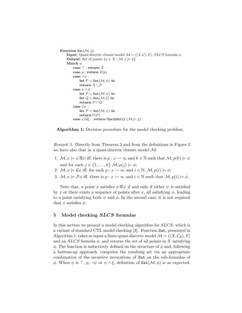
Function Sat(M, φ)Input: Quasi-discrete closure model M = ((X, C),V), SLCS formula φOutput: Set of points {x ∈ X | M, x |= φ}Match φ

case > : return Xcase p : return V(p)case ¬ψ :

let P = Sat(M, ψ) inreturn X \ P

case ψ ∧ ξ :let P = Sat(M, ψ) inlet Q = Sat(M, ξ) inreturn P ∩Q

case ♦ψ :let P = Sat(M, ψ) inreturn C(P )

case ψ Uξ : return CheckUntil (M,ψ, ξ)

Algorithm 1: Decision procedure for the model checking problem.

Remark 3. Directly from Theorem 3 and from the definitions in Figure 2we have also that in a quasi-discrete closure model M:

1. M, x |= φRψ iff. there is p : x ∞ and k ∈ N such thatM, p(k) |= ψ

and for each j ∈ {1, . . . , k} M, p(j) |= φ;2. M, x |= Gφ iff. for each p : x ∞ and i ∈ N, M, p(i) |= φ;

3. M, x |= Fφ iff. there is p : x ∞ and i ∈ N such that M, p(i) |= φ.

Note that, a point x satisfies φRψ if and only if either ψ is satisfiedby x or there exists a sequence of points after x, all satisfying φ, leadingto a point satisfying both ψ and φ. In the second case, it is not requiredthat x satisfies φ.

5 Model checking SLCS formulas

In this section we present a model checking algorithm for SLCS, which isa variant of standard CTL model checking [3]. Function Sat, presented inAlgorithm 1, takes as input a finite quasi-discrete modelM = ((X, CR),V)and an SLCS formula φ, and returns the set of all points in X satisfyingφ. The function is inductively defined on the structure of φ and, followinga bottom-up approach, computes the resulting set via an appropriatecombination of the recursive invocations of Sat on the sub-formulas ofφ. When φ is >, p, ¬ψ or ψ ∧ ξ, definition of Sat(M, φ) is as expected.

Function CheckUntil (M,ψ, ξ)let V = Sat(M, ψ) inlet Q = Sat(M, ξ) invar T := B+(V ∪Q)while T 6= ∅ do

T ′ := ∅for x ∈ T do

N := pre(x) ∩ VV := V \NT ′ := T ′ ∪ (N \Q)

T := T ′;return V

Algorithm 2: Checking until formulas in a quasi-discrete closure space.

To compute the set of points satisfying ♦ψ, the closure operator C of thespace is applied to the set of points satisfying ψ.

When φ is of the form ψ Uξ, function Sat relies on the functionCheckUntil defined in Algorithm 2. This function takes as parametersa model M and two SLCS formulas ψ and ξ and computes the set ofpoints in M satisfying ψ Uξ by removing from V = Sat(M, ψ) all thebad points. A point is bad if there exists a path passing through it, thatleads to a point satisfying ¬ψ without passing through a point satisfyingξ. Let Q = Sat(M, ξ) be the set of points in M satisfying ξ. To identifythe bad points in V the function CheckUntil performs a backward searchfrom T = B+(V ∪ Q). Note that any path exiting from V ∪ Q has topass through points in T . Moreover, the latter only contains points thatsatisfy neither ψ nor ξ. Until T is empty, function CheckUntil first picksan element x in T and then removes from V the set of (bad) points Nthat can reach x in one step. To compute the set N we use the functionpre(x) = {y ∈ X | (y, x) ∈ R}.6 At the end of each iteration the set T isupdated by considering the set of new discovered bad points.

Lemma 4. Let X a finite set and R ⊆ X × X. For any finite quasi-discrete model M = ((X, CR),V) and SLCS formula φ with k operators,Sat terminates in O(k · (|X|+ |R|)) steps.

Theorem 4. For any finite quasi-discrete closure modelM = ((X, C),V)and SLCS formula φ, x ∈ Sat(M, φ) if and only if M, x |= φ.

6 Function pre can be pre-computed when the relation R is loaded from the input.

���� ����

����

����

����������

Fig. 3. A maze.

���� ���

����������

����������

����

���

����������

Fig. 4. Model checker output.

6 A model checker for spatial logics

The algorithm described in Section 5 is available as a proof-of-concepttool7. The tool, implemented using the functional language OCaml, con-tains a generic implementation of a global model-checker using closurespaces, parametrised by the type of models.

An example of the tool usage is to approximately identify regionsof interest on a digital picture (e.g., a map, or a medical image), usingspatial formulas. In this case, digital pictures are treated as quasi-discretemodels in the plane Z × Z. The language of propositions is extended tosimple formulas dealing with colour ranges, in order to cope with imageswhere there are different shades of certain colours.

In Figure 3 we show a digital picture of a maze. The green area is theexit. The blue areas are start points. The input of the tool is shown inFigure 5, where the Paint command is used to invoke the global modelchecker and colour points satisfying a given formula. Three formulas,making use of the until operator, are used to identify interesting areas.The output of the tool is in Figure 4. The colour red denotes start pointsfrom which the exit can be reached. Orange and yellow indicate the tworegions through which the exit can be reached, including and excludinga start point, respectively.

In Figure 6 we show a digital image8 depicting a portion of the mapof Pisa, featuring a red circle which denotes a train station. Streets ofdifferent importance are painted with different colors in the map. Themodel checker is used to identify the area surrounding the station which

7 Web site: http://www.github.com/vincenzoml/slcs.8 c©OpenStreetMap contributors – http://www.openstreetmap.org/copyright.

Let reach(a,b) = !( (!b) U (!a) );

Let reachThrough(a,b) = a & reach((a|b),b);

Let toExit = reachThrough(["white"],["green"]);

Let fromStartToExit = toExit & reachThrough(["white"],["blue"]);

Let startCanExit = reachThrough(["blue"],fromStartToExit);

Paint "yellow" toExit;

Paint "orange" fromStartToExit;

Paint "red" startCanExit;

Fig. 5. Input to the model checker.

Fig. 6. Input: the map of a town. Fig. 7. Output of the tool.

is delimited by main streets, and the delimiting main streets. The outputof the tool is shown in Figure 7, where the station area is coloured inorange, the surrounding main streets are red, and other main streets arein green. We omit the source code of the model checking session for spacereasons (see the source code of the tool). As a mere hint on how practicalit is to use a model checker for image analysis, the execution time onour test image, consisting of about 250000 pixels, is in the order of tenseconds on a standard laptop equipped with a 2Ghz processor.

7 Conclusions and Future Work

In this paper, we have presented a methodology to verify properties thatdepend upon space. We have defined an appropriate logic, stemming fromthe tradition of topological interpretations of modal logics, dating back toearlier logicians such as Tarski, where modalities describe neighbourhood.The topological definitions have been lifted to a more general setting, alsoencompassing discrete, graph-based structures. The proposed framework

has been extended with a spatial variant of the until operator, and we havealso defined an efficient model checking procedure, which is implementedin a proof-of-concept tool.

As future work, we first of all plan to merge the results presented inthis paper with temporal reasoning. This integration can be done in morethan one way. It is not difficult to consider “snapshot” models consistingof a temporal model (e.g., a Kripke frame) where each state is in turna closure model, and atomic formulas of the temporal fragment are re-placed by spatial formulas. The various possible combinations of temporaland spatial operators, in linear and branching time, are examined for thecase of topological models and basic modal formulas in [18]. Snapshotmodels may be susceptible to state-space explosion problems as spatialformulas could need to be recomputed at every state. On the other hand,one might be able to exploit the fact that changes of space over time areincremental and local in nature. Promising ideas are presented both in[17], where principles of “continuous change” are proposed in the settingof closure spaces, and in [20] where spatio-temporal models are gener-ated by locally-scoped update functions, in order to describe dynamicsystems. In the setting of collective adaptive systems, it will be certainlyneeded to extend the basic framework we presented with metric aspects(e.g., distance-bounded variants of the until operator), and probabilis-tic aspects, using atomic formulas that are probability distributions. Athorough investigation of these issues will be the object of future research.

A challenge in spatial and spatio-temporal reasoning is posed by re-cursive spatial formulas, a la µ-calculus, especially on infinite structureswith relatively straightforward generating functions (think of fractals, orfluid flow analysis of continuous structures). Such infinite structures couldbe described by topologically enhanced variants of ω-automata. Classesof automata exist living in specific topological structures; an example isgiven by nominal automata (see e.g., [4,14,21]), that can be defined usingpresheaf toposes [13]. This standpoint could be enhanced with notions ofneighbourhood coming from closure spaces, with the aim of developing aunifying theory of languages and automata describing space, graphs, andprocess calculi with resources.

References

1. M. Aiello. Spatial Reasoning: Theory and Practice. PhD thesis, Institute of Logic,Language and Computation, University of Amsterdam, 2002.

2. M. Aiello, I. Pratt-Hartmann, and J. van Benthem, editors. Handbook of SpatialLogics. Springer, 2007.

3. C. Baier and J.P. Katoen. Principles of model checking. MIT Press, 2008.4. M. Bojanczyk, B. Klin, and S. Lasota. Automata with group actions. In LICS,

pages 355–364. IEEE Computer Society, 2011.5. L. Bortolussi, J. Hillston, D. Latella, and M. Massink. Continuous approximation

of collective system behaviour: A tutorial. Perform. Eval., 70(5):317 – 349, 2013.6. L. Caires and L. Cardelli. A spatial logic for concurrency (part I). Information

and Computation, 186(2):194–235, 2003.7. L. Cardelli, P. Gardner, and G. Ghelli. A spatial logic for querying graphs. In

ICALP, volume 2380 of LNCS, pages 597–610. Springer, 2002.8. L. Cardelli and A.D. Gordon. Anytime, anywhere: Modal logics for mobile ambi-

ents. In POPL, pages 365–377. ACM, 2000.9. A. Chaintreau, J. Le Boudec, and N. Ristanovic. The age of gossip: Spatial mean

field regime. SIGMETRICS, pages 109–120, New York, NY, USA, 2009. ACM.10. Vincenzo Ciancia, Diego Latella, Michele Loreti, and Mieke Massink. Specifying

and verifying properties of space - extended version. CoRR, abs/1406.6393, 2014.11. R. De Nicola, G.L. Ferrari, and R. Pugliese. Klaim: A kernel language for agents

interaction and mobility. IEEE Trans. Software Eng., 24(5):315–330, 1998.12. A. Del Bimbo, E. Vicario, and D. Zingoni. Symbolic description and visual querying

of image sequences using spatio-temporal logic. IEEE Trans. Knowl. Data Eng.,7(4):609–622, 1995.

13. M.P. Fiore and S. Staton. Comparing operational models of name-passing processcalculi. Information and Computation, 204(4):524–560, 2006.

14. M.J. Gabbay and V. Ciancia. Freshness and name-restriction in sets of traces withnames. In FOSSACS, volume 6604 of LNCS, pages 365–380. Springer, 2011.

15. F. Gadducci and A. Lluch-Lafuente. Graphical encoding of a spatial logic for thepi -calculus. In CALCO, volume 4624 of LNCS, pages 209–225. Springer, 2007.

16. A. Galton. The mereotopology of discrete space. In COSIT, volume 1661 of LNCS,pages 251–266. Springer, 1999.

17. A. Galton. A generalized topological view of motion in discrete space. TheoreticalComputer Science, 305(1–3):111 – 134, 2003.

18. R. Kontchakov, A. Kurucz, F. Wolter, and M. Zakharyaschev. Spatial logic +temporal logic = ? In Aiello et al. [2], pages 497–564.

19. V.A. Kovalevsky. Geometry of Locally Finite Spaces: Computer Agreeable Topologyand Algorithms for Computer Imagery. House Dr. Baerbel Kovalevski, 2008.

20. P. Kremer and G. Mints. Dynamic topological logic. In Aiello et al. [2], pages565–606.

21. A. Kurz, T. Suzuki, and E. Tuosto. On nominal regular languages with binders.In FoSSaCS, volume 7213 of LNCS, pages 255–269. Springer, 2012.

22. A. Rosenfeld. Digital topology. The American Mathematical Monthly, 86(8):621–630, 1979.

23. M.B. Smyth and J. Webster. Discrete spatial models. In Aiello et al. [2], pages713–798.

24. J. van Benthem and G. Bezhanishvili. Modal logics of space. In Handbook ofSpatial Logics, pages 217–298. 2007.

25. T. Yung Kong and A. Rosenfeld. Digital topology: Introduction and survey. Com-puter Vision, Graphics, and Image Processing, 48(3):357–393, 1989.