Stephen F. Austin State University Stephen F. Austin State University

SFA ScholarWorks SFA ScholarWorks

Electronic Theses and Dissertations

Winter 12-15-2020

Species Distribution Modeling for Arid Adapted Habitat Species Distribution Modeling for Arid Adapted Habitat

Specialists in Zion National Park Specialists in Zion National Park

Sam Driver Stephen F Austin State University, driversm@jacks.sfasu.edu

Chris M. Schalk Stephen F Austin State University, schalkc@sfasu.edu

Daniel Unger Stephen F Austin State University, unger@sfasu.edu

David Kulhavy Stephen F Austin State University, dkulhavy@sfasu.edu

Follow this and additional works at: https://scholarworks.sfasu.edu/etds

Part of the Desert Ecology Commons, Environmental Studies Commons, Geomorphology Commons,

Natural Resources and Conservation Commons, and the Other Earth Sciences Commons

Tell us how this article helped you.

Repository Citation Repository Citation Driver, Sam; Schalk, Chris M.; Unger, Daniel; and Kulhavy, David, "Species Distribution Modeling for Arid Adapted Habitat Specialists in Zion National Park" (2020). Electronic Theses and Dissertations. 354. https://scholarworks.sfasu.edu/etds/354

This Thesis is brought to you for free and open access by SFA ScholarWorks. It has been accepted for inclusion in Electronic Theses and Dissertations by an authorized administrator of SFA ScholarWorks. For more information, please contact cdsscholarworks@sfasu.edu.

Species Distribution Modeling for Arid Adapted Habitat Specialists in Zion Species Distribution Modeling for Arid Adapted Habitat Specialists in Zion National Park National Park

This thesis is available at SFA ScholarWorks: https://scholarworks.sfasu.edu/etds/354

SPECIES DISTRIBUTION MODELING FOR ARID ADAPTED

HABITAT SPECIALISTS IN ZION NATIONAL PARK

by

Samuel Macon Driver, B.S.

Presented to the Faculty of the Graduate School of

Stephen F. Austin State University

In Partial Fulfillment

of the Requirements

For the Degree of

Master of Science

Stephen F. Austin State University

December 2020

SPECIES DISTRIBUTION MODELING FOR ARID ADAPTED

HABITAT SPECIALISTS IN ZION NATIONAL PARK

by

Samuel Macon Driver, B.S.

APPROVED:

__________________________________________

Dr. Daniel R. Unger, Committee Chair

__________________________________________

Dr. David L. Kulhavy, Committee Member

__________________________________________

Dr. Christopher M. Schalk, Committee Member

__________________________________

Pauline M. Sampson, Ph.D.

Dean of Research and Graduate Studies

i

ABSTRACT

The Arizona toad (Anaxyrus microscaphus) and Jones’ waxy dogbane

(Cycladenia humilis var. jonesii) are habitat specialists with historical ranges in the desert

southwest and specifically, Zion National Park (ZION). The machine learning method,

MaxEnt, constructed species distribution models (SDMs) in ZION for the two study

species at 30 m and 900 m spatial resolutions using climate, topographic, and remotely

sensed data. Additionally, 900 m forecasting models were constructed to observe the

shifts in suitable habitat for the years 2050 and 2070, based off two representative

concentration pathway scenarios. Results indicate promising predictive power for both

high resolution models (30m) for C. humilis var. jonesii and A. microscaphus with area

under curve (AUC) test analysis of 0.715 and 0.810, respectively. Forecasting models

displayed decreasing suitability for A. microscaphus with both climate scenarios applied

to the model. However, C. humilis var. jonesii habitat increased with future scenarios

applied to the MaxEnt models.

ii

ACKNOWLEDGEMENTS

I’d first like to express my gratitude to Stephen F. Austin State University for

allowing me to develop, pursue, and achieve my academic goals. To all my professors in

the environmental and spatial science divisions at the SFA Forestry Department, I am

beyond grateful for all that you’ve helped me accomplish. To my thesis advisor, Dr.

Daniel Unger, thank you for equipping me with the tools to succeed in my future career

field. Thank you to my thesis committee member, Dr. David Kulhavy, for your guidance

and steadfast belief in me. To my graduate representative, Dr. Yanli Zhang, your intro

GIS class was the first I attended at SFA and your advanced GIS class happened to be my

last at SFA; thank you for keeping my intellectual curiosity up from beginning to end.

And how could I forget my thesis committee member, Dr. Christopher Schalk, thank you

for continuously checking in on my progress and staying on me to learn the ecology

behind species modeling. “Bonesaw is ready!!!”

Special thank you to Dr. Kenneth Farrish and Mary Ramos. Thank you, Shauna,

Adam, and Aven for taking me in for the summer in beautiful Zion National Park while

also planting the seed for this research project. I’ll cherish our adventures for a lifetime

and can’t wait to make more.

Above all, I will never be able to thank my family enough. You constantly believe

in my dreams and have supported me through all my life endeavors. To my brother,

iii

Daniel, thank you for cookin’ up gumbos, smoking briskets, and playing that squeezebox

till them roosters’ crow, and above all, always providing the brightest of outlooks when

the odds seemed stacked up against me. Laissez les bons temps rouler! To my mother and

father, Margaret and Paul, thank you for allowing your adult son to park and live in an

ugly RV for two years in your front yard. On a serious note, words don’t do justice for

how grateful I am to have two amazing role models to always look up to, thank you for

everything.

“The only way to get there son is one mile at a time. This road’s crooked

steep and rocky as she winds.”

– Uncle Steve Hartz

iv

TABLE OF CONTENTS

ABSTRACT ......................................................................................................................... i

ACKNOWLEDGEMENTS ................................................................................................ ii

TABLE OF CONTENTS ................................................................................................... iv

LIST OF FIGURES .......................................................................................................... vii

LIST OF TABLES ........................................................................................................... xiii

INTRODUCTION ...............................................................................................................1

OBJECTIVES ......................................................................................................................7

LITERATURE REVIEW ....................................................................................................8

Zion National Park .......................................................................................................... 8

Arizona Toad (Anaxyrus microscaphus) ....................................................................... 10

Jones’ waxy dogbane (Cycladenia humilis var. jonesii) ............................................... 12

Species Distribution Models ......................................................................................... 15

Niche Concepts ............................................................................................................. 16

Maximum Entropy (MaxEnt) ........................................................................................ 17

Sample Size ................................................................................................................ 19

v

Variable Selection ..................................................................................................... 19

Spatial Scale .............................................................................................................. 20

Spatial Resolution ...................................................................................................... 21

Thresholds ................................................................................................................. 23

Sampling Bias ............................................................................................................ 26

Forecasting ................................................................................................................ 27

METHODS ........................................................................................................................30

Study Area ..................................................................................................................... 30

Occurrence Data ............................................................................................................ 32

Data Acquisition ............................................................................................................ 32

Digital Elevation Model Acquisition ......................................................................... 32

Remote Sensing Acquisition ...................................................................................... 33

Climatic Data Acquisition ......................................................................................... 33

Environmental Variable Justification ............................................................................ 35

Variable Selection ......................................................................................................... 45

Model Parameters .......................................................................................................... 46

Spatial Scale .............................................................................................................. 46

vi

Spatial Resolution ...................................................................................................... 49

MaxEnt Calibration ................................................................................................... 49

Model Performance ....................................................................................................... 51

30-m and 900-m Current Models .............................................................................. 51

Model Forecasting..................................................................................................... 51

RESULTS ..........................................................................................................................53

Model Performance ....................................................................................................... 53

Resolution Comparison ................................................................................................. 62

Future Climate Trends ................................................................................................... 68

DISCUSSION & CONCLUSIONS ...................................................................................77

LITERATURE CITED ......................................................................................................86

VITA ................................................................................................................................104

vii

LIST OF FIGURES

Figure 1. ZION is in southwestern Utah and includes habitat for many threatened and

endangered species, including habitat for C. humilis var. jonesii and the A. microscaphus.

..............................................................................................................................................9

Figure 2. Location of the habitat range generated by the USGS for the Arizona toad

(Anaxyrus microscaphus) in the states of California, Nevada, Utah, New Mexico, and

Arizona. A portion of the habitat range is located inside of ZION (orange). The top-right

inset displays an adult Arizona toad. .................................................................................11

Figure 3. Location of the habitat range generated by the Fish and Wildlife Service for

Jones’ cycladenia (Cycladenia humilis var. jonesii) scattered throughout southeastern

Utah and northern Arizona. Habitat for C. humilis var. jonesii is fragmented and is known

to occur in only southeast Utah and far northern Arizona. The top-left inset displays a

flowering C. humilis var. jonesii........................................................................................13

Figure 4. A demonstration of a representative concentration pathway depicting the four

climate scenarios of (2.6, 4.5, 6.0, and 8.5). RCPs begin to differ from 2025-2030 and are

extrapolated to the year 2100. RCP 2.6 is considered the best-case scenario while RCP

8.5 is the worst-case climate scenario (). ...........................................................................29

viii

Figure 5. ZION is the study area for the SDMs created for A. microscaphus and C.

humilis var. jonesii. The inset in the top right displays the five national parks found

within Utah.........................................................................................................................30

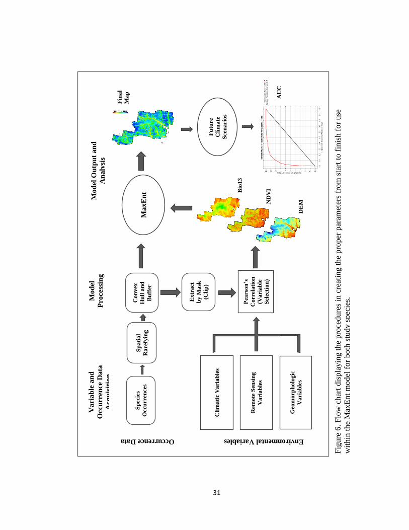
Figure 6. Flow chart displaying the procedures in creating the proper parameters from

start to finish for use within the MaxEnt model for both study species. ...........................31

Figure 7. Digital elevation model for ZION at 30 m resolution. .......................................36

Figure 8. Slope derived from the original DEM for ZION at 30 m resolution. .................37

Figure 9. Aspect derived from the original DEM for ZION at 30 m resolution. ...............39

Figure 10. Terrain ruggedness index derived from the original DEM for ZION at 30 m

resolution............................................................................................................................40

Figure 11. Topographic position index derived from the original DEM for ZION at 30 m

resolution. This variable describes the valley bottom flatness in green and higher

elevation peaks in the red. ..................................................................................................42

Figure 12. Normalized difference vegetation index derived from Landsat 5 satellite

imagery for ZION at 30 m resolution. Green represents vegetation in this map and red

represents lack of vegetation. .............................................................................................43

Figure 13. Bare soil index derived from Landsat 5 satellite imagery for ZION at 30 m

resolution............................................................................................................................44

Figure 14. The model training for A. microscaphus was determined by constructing a 50

km buffer around the occurrence points obtained from GBIF.org. Of the 327 occurrence

points, 87 points remained after spatial rarefying which were used to train the MaxEnt

ix

model. Occurrence localities used inside and outside of ZION were used to train the

SDMs. ................................................................................................................................47

Figure 15. The model training extent was determined by constructing a 50 km buffer

around the occurrence points obtained from GBIF.org. Spatial rarefying was not

conducted on the occurrence points for C. humilis var. jonesii due to the low volume of

occurrence localities...........................................................................................................48

Figure 16. A. The average receiver operating curve (AUC) for A. microscaphus with the

five replicates run in MaxEnt. The red line representing the fit of the model to the

training data. The blue line represents the fit of the model to the 25% testing data. AUC

over 0.7 assumes positive predictive power for the model. B. Represents the test omission

rate and predicted area as a function of the cumulative threshold. ....................................54

Figure 17. A. The average receiver operating curve (AUC) for C. humilis var. jonesii with

the five replicates run in MaxEnt. The red line representing the fit of the model to the

training data. The blue line represents the fit of the model to the 25% testing data. AUC

over 0.7 assumes positive predictive power for the model. B. Represents the test omission

rate and predicted area as a function of the cumulative threshold. ....................................55

Figure 18. Partial dependence plots displaying the marginal response of the 12

environmental variables selected for A. microscaphus in the MaxEnt model. Each

response curve demonstrates the range of suitability for each environmental variable if

each variable were used to create a MaxEnt model independent of other variables. ........57

x

Figure 19. Partial dependence plots displaying the marginal response of the 13

environmental variable selected for Cycladenia humilis var. jonesii in the MaxEnt model.

Each response curve demonstrates the range of suitability for each environmental

variable if each variable were used to create a MaxEnt model independent of other

variables. ............................................................................................................................59

Figure 20. MaxEnt model output for 30 m resolution habitat suitability maps for A.

microscaphus in ZION. Suitability classes describe the ranking of habitat preference for

the species being modeled. Models were created using MaxEnt.......................................60

Figure 21. MaxEnt model output for 30 m resolution habitat suitability maps for C.

humilis var. jonesii in ZION. Suitability classes describe the ranking of habitat preference

for the species being modeled. Models were created using ArcMap and MaxEnt. ...........61

Figure 22. MaxEnt habitat suitability outputs for A. microscaphus with differing

resolution sizes to compare low to high suitability habitat for ZION. Highest suitability

habitat increased within the park with the higher resolution. All environmental variables

(topographic, remotely-sensed, and climate) were applied to these two outputs. .............66

Figure 23. MaxEnt habitat suitability outputs for C. humilis var. jonesii with differing

resolution sizes to compare low to high suitability habitat for ZION. Highest suitability

habitat decreased within the park with the higher resolution. All environmental variables

(topographic, remotely-sensed, and climate) were applied to these two maps. .................67

Figure 24. Forecasting SDM of A. microscaphus contrasting the suitable habitat for future

climate scenarios for representative concentration pathways that describe greenhouse gas

xi

concentration of 2.6 W/m2 and 8.5 W/m2 for the year 2050. The SDM covers the

complete training extent of the toad to better understand changes in suitable habitat (see

Figure 14). The ‘10 percentile training presence’ threshold was used to delineate suitable

habitat in this analysis. .......................................................................................................69

Figure 25. Forecasting SDM of A. microscaphus contrasting the suitable habitat for

climate scenarios for representative concentration pathways, which describe greenhouse

gas concentration of 2.6 W/m2 and 8.5 W/m2 for the year 2070 (see Figure 14). The SDM

covers the complete training extent of the toad to better understand changes in suitable

future habitat. The ‘10 percentile training presence’ calculated by the MaxEnt output was

used as the threshold to delineate suitable habitat. ............................................................70

Figure 26. Forecasting SDM of A. microscaphus for the current year (2020) and 2050

using binary distribution of suitable versus not suitable habitat. The ‘10 percentile

training presence’ threshold was calculated by MaxEnt to delineate suitable habitat in this

analysis. ..............................................................................................................................71

Figure 27. Forecasting SDM of A. microscaphus for the current year (2020) and 2070

using binary distribution of suitable versus not suitable habitat. The ‘10 percentile

training presence’ threshold was calculated by MaxEnt to delineate suitable habitat in this

analysis. ..............................................................................................................................72

Figure 28. Forecasting SDM of C. humilis var. jonesii contrasting the suitable habitat for

future climate scenarios for representative concentration pathways that describe

greenhouse gas concentration of 2.6 W/m2 and 8.5 W/m2 for the year 2050. The SDM

xii

covers the complete training extent of the plant to better understand changes in suitable

future habitat (see Figure 15). The ‘10 percentile training presence’ calculated by the

MaxEnt output was used to delineate suitable habitat in this analysis. .............................73

Figure 29. Forecasting SDM of C. humilis var. jonesii contrasting the suitable habitat for

future climate scenarios for with representative concentration pathways that describe

greenhouse gas concentration of 2.6 W/m2 and 8.5 W/m2 for the year 2070. The SDM

covers the complete training extent of the plant to better understand changes in suitable

habitat (see Figure 15). The ‘10 percentile training presence’ calculated by the MaxEnt

output was used to delineate suitable habitat in this analysis. ...........................................74

Figure 30. Forecasting SDM of C. humilis var. jonesii in ZION for the current year

(2020) and 2050 using binary distribution of suitable versus not suitable habitat. The ‘10

percentile training presence’ threshold was calculated by MaxEnt to delineate suitable

habitat in this analysis. .......................................................................................................75

Figure 31. Forecasting SDM of C. humilis var. jonesii in ZION for the current year

(2020) and 2070 using binary distribution of suitable versus not suitable habitat. The ‘10

percentile training presence’ threshold was calculated by MaxEnt to delineate suitable

habitat in this analysis. .......................................................................................................76

xiii

LIST OF TABLES

Table 1. List of the 19 bioclimatic variables taken from the WorldClim database and used

for analysis within the target species’ SDMs. Pearson’s correlation test was first used to

eliminate highly correlated variables with topographic and remotely sensed variables. ...34

Table 2. Results from Pearson’s correlation coefficient used to quantify correlation

among environmental variables. Resulting variables were used to train the model within

MaxEnt. ..............................................................................................................................45

Table 3. The MACHISPLIN package results for the climate variables downscaled to 30

m resolution and the r2 values associated with each layer. Results are based off an

ensemble approach using six algorithms. Independent variables used in the approach

include elevation, slope, aspect, and topographic wetness index. .....................................50

Table 4. Permutation importance values for each bioclimatic variable within the MaxEnt

model for the 30 m A. microscaphus SDM. The permutation value is determined by

randomly permuting the values of each independent variables against the training points.

Values are then normalized to provide percentages; higher values suggest greater

influence on the model. ......................................................................................................56

Table 5. Permutation importance values for each WorldClim variable for the MaxEnt

model for the 30 m C. humilis var. jonesii SDM. The permutation value is determined by

xiv

randomly permuting the values of each independent variables against the training points.

Values are then normalized to provide percentages; higher values suggest greater

influence on the model. ......................................................................................................58

Table 6. Differing MaxEnt outputs for both study species comparing the contrast ..........63

between 30 m and 900 m resolution. .................................................................................63

Table 7. The percent change between 30 m and 900 m SDM outputs for the study species

within five habitat suitability classes. ................................................................................64

Table 8. Permutation importance values for each bioclimatic variable within the MaxEnt

model for the 900 m A. microscaphus and C. humilis var. jonesii SDMs. The permutation

value is determined by randomly permuting the values of each independent variables

against the training points. Values are then normalized to provide percentages; higher

values suggest greater influence on the model. .................................................................65

Table 9. Area of suitable habitat for A. microscaphus within the training extent for future

climate scenarios for 2050 and 2070 with differing RCPs of 2.6 and 8.5 W/m2. ..............70

Table 10. Area of suitable habitat for A. microscaphus within ZION for current and future

climate scenarios of 2050 and 2070 with differing RCPs of 2.6 and 8.5 W/m2. ...............72

Table 11. Area of suitable habitat for C. humilis var. jonesii within the training extent for

future climate scenarios of 2050 and 2070 with differing RCPs of 2.6 and 8.5 W/m2. .....74

Table 12. Area of suitable habitat for C. humilis var. jonesii within ZION for future

climate scenarios of 2050 and 2070 with differing RCPs of 2.6 and 8.5 W/m2. ...............76

1

INTRODUCTION

Since the incorporation of new statistical methods and GIS tools, the development

of predictive species distribution models (SDMs) has expanded in the field of ecology,

biogeography, and conservation biology (Raes, 2012). SDMs describe how climatic and

environmental factors relate to species occurrences in geographic space, in order to

delineate suitable habitat over local, regional, and global scales. Common applications for

SDMs include projecting species distribution for current, past, and future climates,

studying relationships between environmental parameters and species richness, mapping

invasive species habitat range, and conservation planning (Melo-Merino et al., 2020).

Of notable interest from a conservation and management standpoint, is the

construction of SDMs to understand the current and future distribution of available

habitat for species, particularly habitat specialist. Habitat specialists display a narrow

range of environmental factors and have relatively limited geographic requirements, often

constricting the species to a defined range of suitable habitats for which they are well-

adapted (Hernandez et al., 2006; Büchi and Vuilleumier, 2014). In their optimal habitat, it

is believed that specialists perform better than generalists, with a trade-off to generalists

on performance and fitness in suboptimal habitats (Levins, 1968; Lawlor and Smith

1976; Marvier et al. 2004; Jasmin and Kassen 2007). However, alterations to resource

1

gradients can lead to unfavorable impacts on specialists. Specialist species are susceptible

to anthropogenic factors, such as climate change and urbanization (McKinney and

Lockwood, 1999). Interspecific competition also contributes to specialization within a

species (Biedma et al. 2019). Generalists can alter ecosystems by outcompeting

specialists, homogenizing ecosystems, and reducing biodiversity at the community level

(Büchi and Vuilleumier, 2013). These reductions in availability and resources can

fragment the available habitat, resulting in demographic isolation, population decline,

species extirpation, and ultimately leading to biodiversity loss (Vrba, 1987; Ricketts,

2001; Büchi and Vuilleumier, 2013). Monitoring the loss of biodiversity, especially

within specialist species is important to understand the identity, abundance, and shifts in

their habitat range (Díaz et al., 2006).

Due to the effects of climate change and other factors on desert landscapes,

understanding the available habitat to specialist species is of particular importance (IPCC,

2014). Globally, desert climates are changing faster than other non-polar terrestrial

ecosystems due to climate change (IPCC, 2014). Increased effects of climate change are

projected across the desert southwest in the 21st century with increases in aridity and

temperatures, along with longer drought durations (Cayan et al., 2010; Dominguez et al.,

2010; Seager and Vecchi, 2010). Arid environments, such as the desert southwest of the

United States, provide an array of ecosystems and microclimates conducive to examine

the current and projected availability of habitats for specialist species. Across regions of

the southwest, seasonal precipitation is erratic and prolonged droughts are common,

2

leading to adverse effects on landscape and ecosystems (Notaro et al., 2011). These

abiotic factors have shifted species to become better adapted to their xeric landscape.

Plants have become drought tolerant by growing deeper tap roots, inducing seed

dormancy, or utilizing paraheliotropism to minimize sun exposure (Canadell et al., 1996;

Chávez et al., 2016). Desert anurans have adapted to diminishing water resources by

becoming fossorial, utilizing explosive breeding behaviors, accelerating metamorphosis,

and becoming restricted geographically to stable water sources (Kulkarni et al., 2011;

Schalk et al., 2015).

To better understand species habitat requirements and the effects of future climate

change scenarios on species, researchers use SDMs such as the maximum entropy

modeling method (MaxEnt) to analyze these changes (Elith et al., 2010). MaxEnt is a

machine-learning technique used in modeling the distribution of a species’ habitat using

presence-only occurrence records (Phillips et al., 2006). The maximum entropy algorithm

attempts to estimate a probability distribution of species occurrence that is closest to

uniform while maintaining its environmental constraints (Elith et al., 2010). MaxEnt has

become a popular platform for species distribution modelling because of an ease of use

interface, implementation of presence-only data, low occurrence data requirements,

future forecasting ability, and its use of environmental data from across the study area

rather than a discriminative approach (Phillips and Elith, 2013). MaxEnt is also capable

of projecting one set of environmental layers to other locations using similarly formatted

environmental layers. Projecting is often used to map species in areas of changing

3

climate, observing potential habitat for invasive species, or building models in unknown

areas for target species evaluation (Phillips, 2017). MaxEnt is capable of handling both

continuous and categorical (discrete) environmental variables within its algorithm

(Phillips and Dudík, 2008). Using both continuous and categorical environmental data,

occurrence locations of the target species are then included into the MaxEnt algorithm to

build a model that projects a species habitat range across a geographic landscape to

identify other potential locations of suitable habitat.

With changing climates and diminishing habitats for many species, forecasting

SDMs has become a powerful tool for conservation practitioners and resource managers

as changing climates impact ecological systems (Guisan et al. 2013). MaxEnt can

construct SDMs to predict the changes in the geographic distribution of a species under

different climate change scenarios. These climate change scenarios are represented by

representative concentration pathways (RCPs), which are the developments of scenario

sets containing emissions, concentrations, and land-use trajectories (Vuuren et al., 2011).

RCPs project a potential future scenario and allow SDMs, such as MaxEnt, to capture the

shifts in suitable habitat for a species. This provides an invaluable tool for proactively

monitoring and planning conservation efforts for specialist species who are at risk of

extirpation and declining habitat due to changing climates.

One of the most diverse protected landscapes in the desert southwest, Zion

National Park (ZION) provides refuge to various protected species within its boundaries.

ZION was chosen as the study area due to its diverse landscape characterized by high

4

plateaus and deep sandstone canyons carved out by the Virgin River and additional

tributaries which support many microclimates. The southern section of the park is

characterized by desert habitat while the norther portion of the park is covered with high

plateau forests (US DOI, 2013a). An abundance of specialist species inhabit the park,

including the Arizona toad (Anaxyrus microscaphus), desert tortoise (Gopherus

agassizii), Gila monster (Heloderma suspectum), and Mexican spotted owl (Strix

occidentalis lucida) (US DOI, 2009; US DOI, 2013a). These and many other species are

sensitive to environmental alterations occurring such as habitat degradation, invasive

species encroachment, changes in hydrologic regimes, and rising temperatures due to

climate change (Ryan et al., 2014). To protect sensitive habitat within the park from the

changes in habitat, ZION complies with the National Environmental Policy Act in

addition to other environmental regulations, including the Endangered Species Act and

the National Historic Preservation Act (US DOI, 2013a).

This study concentrates on the habitat range of two arid adapted habitat specialists

within ZION, the Arizona toad (Anaxyrus microscaphus) and Jones’ waxy dogbane

(Cycladenia humilis var. jonesii) (Tilley et al., 2010; Ryan et al., 2015). Both species are

endemic to the desert southwest and display morphological traits typically found in

regions of prolonged drought and extreme temperatures. Anaxyrus microscaphus is a

habitat specialist that requires slow moving streams, sandy floodplains for burrowing,

and a narrow temperatures range for breeding (Sullivan, 1992; Ryan et al., 2017). Their

habitat is currently threatened by changes in the hydrological cycle, habitat

5

modifications, forest fires, hybridization, and introduced pathogens (Sullivan and Lamb,

1988; Ryan et al., 2014). Reports have shown that on a regional scale, toads are

declining, but locally have more stable populations based upon habitat conditions

(Sullivan, 1993; Bradford et al., 2005; Ryan et al., 2017). The habitat for C. humilis var.

jonesii is highly specialized, requiring gypsiferous and saline soils that are primarily

fragmented rock surfaces with soils at least 50 cm in depth (Welsh et al., 1987; USFWS,

2008). Main threats to C. humilis var. jonesii habitat arise from shifts in climate and land

use practice (Tilley et al., 2010). Populations for C. humilis var. jonesii are currently

geographically disjunct across southeastern Utah, little is known about the taxon’s

historic range (Sipes et al., 1994; Sipes and Wolf, 1997).Suitable habitat currently

remains for both study species inside of ZION, with common sightings of A.

microscaphus along riparian zones and other ephemeral water sources (Dalh et al., 2000).

Unfortunately, there have been no official sightings of C. humilis var. jonesii within the

park. Nearest populations are to the east in Garfield County, Utah and Mohave County,

Arizona (Welsh et al., 1987; Sipes et al. 1994).

Habitat specialists are known to have restricted spatial distribution patterns which

typically leads to limited occurrences localities (Kattan, 1992; Segurado and Araújo,

2004; Elith et al., 2006). Furthermore, SDMs for habitat specialists are known to have

narrow geographic ranges but have higher SDM accuracy than those of generalist species

(Luoto et al., 2005; Elith et al., 2006). Within this study, MaxEnt is used to capture the

distribution of A. microscaphus and C. humilis var. jonesii, with differing spatial

6

resolutions providing detail into the estimation of suitable habitat for higher resolution

models. Forecasting models with MaxEnt also observed the long-term habitat shifts due

to abiotic factors within the region and ZION.

7

OBJECTIVES

The goal of this study is to develop a SDM for arid adapted habitat specialist

species within ZION using the maximum entropy modelling methods (MaxEnt).

Generating reliable SDMs will benefit environmental managers in mapping valuable

species habitat to help establish a firm ecological background to assist in understanding

complex management issues. Below are the following objectives for the study:

1. Create a species distribution model for both the Arizona toad (Anaxyrus

microscaphus) and Jones’ Waxy Dogbane (Cycladenia humilis var. jonesii) to

delineate suitable habitat range within the ZION boundaries using the MaxEnt

software to construct ecologically relevant climate, topographic, and remotely

sensed variables to maximize effectiveness of model strength;

2. Construct SDMs for the target species at 30 m and 900 m spatial resolutions

within ZION, for comparison of model strength between the two resolutions; and

3. Utilize forecasting techniques to project each species’ distribution for the years

2050 and 2070 to understand the effect of climate change on habitat suitability for

the target species based on 2.6 and 8.5 W/m2 RCP scenarios. Future habitat

scenarios will be estimated by representative concentration pathways that predict

the measurement of greenhouse gas concentration for alternative future climates.

8

LITERATURE REVIEW

Zion National Park

ZION is in southwestern Utah (Figure 1) within Washington, Iron, and Kane

counties. ZION entered the national park system in 1919 under the signing of President

Woodrow Wilson. The park has an area of 601.9 km2, with 84% designated as wilderness

(US DOI, 2013a). The park is located at the juncture of the Colorado Plateau, Mojave

Desert, and Great Basin ecoregions. The elevation ranges from 2,660 m at its highest

point (Horse Ranch Mountain) to 1,117 meters (Coal Pits Wash) at its lowest point (US

DOI, 2013a). More than 1,000 plant species inhabit ZION with approximately 78 species

of mammals, 30 reptile species, 7 amphibians, 8 fish, and 291 species of birds (NPS,

2018). The last known stable population studied in ZION was located along the Virgin

River and Oak Creek riparian zones from 1998-1999 (Dahl et al., 2000). They are

believed to still inhabit the park, though no recent studies can support this claim. There is

no known literature of C. humilis var. jonesii populations occurring inside of ZION, only

potential suitable habitat remains within the park boundaries for the plant (US DOI,

2013b).

9

Figure 1. ZION is in southwestern Utah and includes habitat for many

threatened and endangered species, including habitat for C. humilis

var. jonesii and the A. microscaphus.

10

Arizona Toad (Anaxyrus microscaphus)

Anaxyrus microscaphus was originally described by Cope (1867) as Bufo

microscaphus. The toads’ habitat range expands primarily along the Mogollon Plateau in

western New Mexico, expanding through Arizona into far southwestern Utah and eastern

Nevada along the Virgin and Colorado River basins and its tributaries (Figure 2) (Dodd,

2013; Blais et al., 2016). Aside from the Virgin and Colorado River locations, historical

occurrences for the toad have been found in the Agua Fria, Salt, Verde, Bill Williams,

and Hassayampa Rivers in Arizona and the Gila, Mimbres, and San Francisco Rivers in

New Mexico (Sullivan and Lamb, 1988; Ryan et al., 2015). In New Mexico, roughly

70% of historical sites monitored for A. microscaphus recorded no observations in past

decades, implying a decline in New Mexico populations over that time span (Ryan et al,

2017). Monitoring of A. microscaphus populations by Ryan et al. (2017) between 2013

and 2016 along the Gila and San Francisco River showed that toad populations were

stable within those years, although local populations were vulnerable to local extirpation,

mainly due to random weather events. Currently, A. microscaphus is considered a

Species of Greatest Conservation Need in New Mexico and a state ‘sensitive’ species in

Arizona, Nevada, and Utah (New Mexico DGF, 2006; Dodd, 2013).

The toad is found at elevations of 365-2700 m and typically occupies marginal

zones or terraces, preferring mixtures of dense willow clumps and open flats or flood

channels (Sweet, 1992). Toads are typically observed from February to September where

they enter torpor for winter months (Schwaner and Sullivan, 2009). During the breeding

11

Fig

ure

2. L

oca

tion o

f th

e hab

itat

ran

ge

gen

erat

ed b

y t

he

US

GS

for

the

Ari

zona

toad

(Anaxy

rus

mic

rosc

aphus)

in t

he

stat

es o

f C

alif

orn

ia, N

evad

a, U

tah, N

ew M

exic

o, an

d

Ari

zona.

A p

ort

ion o

f th

e hab

itat

ran

ge

is l

oca

ted i

nsi

de

of

ZIO

N (

ora

ng

e).

The

top

-rig

ht

inse

t dis

pla

ys

an a

dult

Ari

zona

toad

.

12

season, males begin their calling when air temperatures range anywhere from 8 to 18°C

(Sullivan, 1992). Arizona toads remain close to flowing water sources during warmer

months and seldom migrate further than 200 m, typically remaining within floodplain

habitat (Schwaner and Sullivan, 2005). Clutch size average is around 4,500 eggs per

clutch and eggs are deposited in riparian areas of streams, shallows, backwashes, and

side-pools, where they hatch anywhere from 3-6 days (Blair, 1955; Schwaner and

Sullivan, 2005). Under normal conditions, tadpoles require relatively shallow, slow

flowing streams, and avoid faster moving water (Ryan et al, 2017).

Jones’ waxy dogbane (Cycladenia humilis var. jonesii)

Jones’ waxy dogbane is found in southern Utah counties (Emery, Grand, Garfield,

and Kane Counties) and Northern Arizona (Figure 3), occurring at a narrow range of

latitudes between 36° and 39° north (USFWS, 2008). Cycladenia humilis var. jonesii can

be found at elevations ranging from 1,300-1,800 meters on side slopes or at the base of

mesas, and typically within plant communities of mixed desert scrub, juniper, or wild

buckwheat-Mormon tea receiving 6 to 9 inches of mean annual precipitation (Tilley et

al., 2010). Cycladenia humilis var. jonesii is a long-lived herbaceous perennial in the

Dogbane family and grows 10-15 cm in height (USFWS, 2008). Flowering of the plant

takes place typically in April through June and produces a pink or rose-colored, trumpet

shaped flower. Soil requirements are edaphic and most if not all plants are found in

gypsiferous and saline soils of the Cutler, Summerville, and Chinle formations (USFWS,

2008). Often, habitat has been found on (80 to 100%) rock fragments, with shallow soils

13

Fig

ure

3. L

oca

tion o

f th

e hab

itat

ran

ge

gen

erat

ed b

y t

he

Fis

h a

nd W

ildli

fe S

ervic

e fo

r

Jones

’ cy

clad

enia

(C

ycla

den

ia h

um

ilis

var

. jo

nes

ii)

scat

tere

d t

hro

ug

ho

ut

south

east

ern

Uta

h a

nd n

ort

her

n A

rizo

na.

Hab

itat

for

C. hum

ilis

var

. jo

nes

ii i

s fr

agm

ente

d a

nd i

s know

n

to o

ccur

in o

nly

south

east

Uta

h a

nd f

ar n

ort

her

n A

rizo

na.

The

top

-lef

t in

set

dis

pla

ys

a

flow

erin

g C

. hum

ilis

var.

jones

ii.

14

less than 50 cm deep (Welsh et al., 1987). Cycladenia humilis replicates mainly by the

spreading of its rhizomes rather than by sexual reproduction, according to a study by

Sipes et al. (1994), supporting the theory of a lack of active primary pollinators to the

flower. It overwinters as a subterranean rhizome and is considered rhizomatous, meaning

it contains a long underground stem system not viewable from the ground surface.

Because C. humilis var. jonesii is a rhizomatous plant species it is made up of ramets,

which is an underground system of genetically identical individuals, the colony of ramets

makes up a genet (Sipes and Tepedino, 1996; USFWS, 2008).

Cycladenia humilis is a genus with three varieties currently recognized within the

species: C. humilis var. humilis, C. humilis var. venusta, and C. humilis var. jonesii.

Cycladenia humilis var. humilis is endemic to northern California while C. humilis var.

venusta is endemic to southern California (Hickman, 1993). Results from a study by

Brabazon (2015) supports the variation of jonesii indicates significant genetic structure,

supporting a possible delineation of jonesii as its own distinct species apart from the two

California variations. Cycladenia humilis var. jonesii was listed as a threatened species in

June of 1986 with an estimated total of 7,500 known individuals in the habitat range

during that time. As of 2008, there is believed to only be 1,100 individuals (Sipes and

Tepedino, 1996). Threats to C. humilis var. jonesii habitat are anthropogenic in nature

with disturbances including off-highway vehicle (OHV), oil and gas exploration,

livestock grazing, and the threat of rising temperatures due to climate change (Welsh et

al., 1987; Sipes et al., 1994). According to the recovery plan documented by FWS,

15

further monitoring and implementing of management plans for conservation of habitat is

currently being conducted (USFWS, 2008).

Species Distribution Models

SDM or environmental niche model (ENM) is an algorithmic method for the

modeling of a species habitat range based on the correlation between known occurrences

and the environmental conditions of occurrence localities (Elith and Leathwick, 2009). In

a Grinnellian sense, habitat modelling of an organism is adapted to tolerance zones or

niches, which are considered abiotic requirements in which a species is capable of

surviving within (Lorini and Vail, 2015). The utilization of species modelling has become

ubiquitous in many fields, especially those of analytical biology and can be used

extensively in conservation, natural resource management, ecology, evolution, and

invasive-species management (McShea, 2014; Pollock et al., 2014).

Among many types of models used in mapping species range habitat, some of the

more prevalently known statistical models fall under regression-based techniques, such

as: generalized linear model (GLM), generalized additive models (GAM), and

multivariate adaptive regression splines (Guisan et al., 2002; Elith and Leathwick, 2007).

The advancement of these particular analyses pioneered the development and growth of

innovative statistical methods and led to a renaissance of mechanistic models and

machine learning approaches. Between the years of 1992 and 2010 the increase in

published SDM related articles in ecological literature has increased from ten articles in

1992 up to 350 articles per year in 2010 (Brotons, 2014). As of 2019, the increase on

16

mendely.com has risen to 2,769 published articles on species distribution modelling.

Increasing in popularity, with the aid of highly effective computer system machine

learning techniques like those of MaxEnt, artificial neural networks (ANN), Genetic

algorithm for rule set production (GARP), boosted regression trees (BRT), random forest

(RF), support vector machines (SVM), and also ensemble models (Pearson et al., 2002;

Phillips et al., 2006; Elith et al., 2008; Evans et al., 2011; Grenouillet et al., 2011). Many

factors have contributed to the quick growth in the usage of species distribution

modelling such as the expanding accessibility in occurrence databases like that of

websites like International Union for Conservation of Nature (IUCN), iNaturalist, Global

Biodiversity Information Facility (GBIF), Biodiversity Heritage Library, Birdlife

International, or FishBase. These species occurrence databases are typically open source

websites that accumulate data by use of citizen scientists, uploading species sightings to

the website with exact coordinate location and additional detailed locality data.

Digitization of historical museum specimens has also contributed to the expanding

database collection for species occurrences.

Niche Concepts

Arauijo and Guisan (2006) proposed that one of the biggest challenges and most

overlooked elements of modelling species distribution is understanding and clarifying the

niche concept. Recognizing the differences between a fundamental niche and realized

niche is vital in comprehending the fluidity of the ever-shifting interactions with

interspecific interactions (i.e. predation, competition, mutualism). A Hutchinsonian

17

definition of a fundamental niche is the set of all conditions that allow for a species long-

term survival in the absence of competition, whereas a realized niche is a subset of the

fundamental niche that the species currently occupies with the presence of competition.

Chase and Leibold (2003) proposed a contrarian approach to defining a niche by

excluding the idea of a fundamental niche and realized niche altogether, they stated a

niche is limited by environmental factors that allows a population to reproduce at a rate

that is higher than the rate of mortality. Ambiguity on what a model represents often

results in misleading or inaccurate models. Soberón and Peterson (2005) supported the

idea that niche models provide an approximation of the species’ fundamental niche.

Conversely, other researchers have supported that models are spatial representations of

the realized niche (Guisan and Zimmerman, 2000; Pearson et al., 2002). Whether or not a

model represents a fundamental niche or a realized niche, the condition is dependent on

the parameters, variables, and algorithm representing the range in which a species

occupies.

Maximum Entropy (MaxEnt)

The principle of maximum entropy was presented by Edwin Thompson Jaynes in

1957, and since has helped expand disciplines such as thermodynamics, economics,

forensics, and ecology. MaxEnt software became available in 2004 and is a general-

purpose statistical machine-learning algorithm for making predictions from incomplete

datasets using presence-only data. MaxEnt contrasts presence data against background

samples, which are often called pseudo-absences (Phillips et al., 2009). Entropy is a

18

concept in information theory that measures the amount of information lost when the

value of a random variable is not known (Shannon, 1948). Lowering this amount of

entropy is key in developing a strong model. The more background information that we

have available the more entropy is lowered and the more uncertainty is reduced.

Increasing the data that indicates a species is present within an environment of ecological

conditions is information that will theoretically reduce the entropy within the model.

Within the MaxEnt model, entropy is measured on a grid cell (raster), the grid cell is

made up of pixels and within each pixel an occurrence point is either present or absent.

Any pixel that contains an occurrence point would be expected to demonstrate a

relatively low amount of entropy, while a pixel absent of an occurrence point would be

expected to have a high level of entropy (Phillips and Dudík, 2008). Occurrence points

are any coordinates denoting localities of where a particular species has been previously

recorded, typically using latitude and longitude. Many of these occurrence points are

derived from historical museum records or citizen science websites.

After each completion of a model, MaxEnt computes the area under the receiver

operating characteristic curve (AUC) as a tool for evaluating the predicted distribution of

species in a model. AUC was first developed for radar signal detection before being used

in medical research field and later accepted as the standard for assessing accuracy of

SDMs (Pepe, 2000; Jiménez-Valverde, 2012). Li and He (2018) proposed an approximate

guide for classifying the accuracy of AUC on scale ranging from 0-1: 0.90–1.00 =

excellent, 0.80–0.90 = good, 0.70–0.80 = fair, 0.60–0.70 = poor, and 0.50–0.60 = fail.

19

AUC values characterize the model’s ability to distinguish presence records from

background data.

Sample Size

Sample size in a species distribution model refers to the quantity of occurrence

point data collected for a species. The effects of sample size on a model are often weakly

considered in SDMs but can greatly influence the success rate of predicting suitable

species habitat (Stockwell and Peterson, 2002). Depending on the rarity of the species,

there is often a limit on occurrence data and exceptions must be implemented in

situations dealing with low occurrence records. Model performance is known to decrease

with samples sizes smaller than 15 and decrease dramatically for sample sizes smaller

than five (Pearson et al., 2006; Papeş and Gaubert, 2007). With small sample sizes,

outliers carry more weight in analyses, whereas more occurrence points help balance

outlier effects (Wisz et al., 2008). Also, uncertainty related to parameter estimates (e.g.

means, modes, medians) decrease with an increase in sample size (Crawley, 2002).

Though many model techniques are available, Hernandez et al. (2006) concluded in a

study that MaxEnt is the most capable in producing useful model results with smaller

sample sizes.

Variable Selection

Selection of environmental variables for SDMs should correspond with a deep

ideology and understanding of the species biogeography, ecology, population dynamics

and human disturbance. Careful selection of environmental variables is important in

20

producing a high quality, low bias model (Araújo and Guisan, 2006). MaxEnt, along with

many other machine learning models can use topographic, climatic, soil, and remotely

sensed variables. Yiwen et al. (2016) presents two methods for selecting environmental

variables in MaxEnt. The first method consists of selecting environmental variables based

from a priori or pre-selected ecological and biological knowledge. The second approach

utilizes a reiterative process of a stepwise removal of least contributing variables, both

approaches reduce overfitting and increase model accuracy.

In an article produced by Brown (2014) he outlines the use of a computer program

called “SDM Toolbox”, intended to work as a platform connecting both Python and

AcrGIS 10.1 (or higher). The toolbox consists of 59 scripts for use in macroecology,

landscape genetics, landscape ecology, and evolutionary studies. Among the many scripts

in the toolbox is the jackknifing tool, which measures variable importance and

systematically excludes one environmental variable at a time when running the model.

This process informs the user of variable contribution within the model while also

identifying highly correlated variables.

Spatial Scale

Spatial scale, commonly referred to as spatial extent or training range, is simply

the overall size of the study area in an SDM (Turner et. al, 1989). A common challenge

when constructing a species model is determining the appropriate extent of the study

area. Many study areas are determined by geographical or political borders, resulting in

poor model calibration leading to an incomplete range of environmental conditions. This

21

issue can lead to errors when extrapolating beyond the training range or when using

forecasting techniques for future modelling (El-Gabbas and Dormann, 2018).

A study by Williams et al. (2009) implemented a spatial scale design by

producing a 50-km buffer around occurrence points using a convex hull. Likewise,

Brown (2014) implements a convex hull buffer solution by buffering a set distance

around the occurrence points, in most cases 50-km. This helps eliminate overfitting by

reducing the spatial extent range and allows the model to select background points at only

feasible areas of dispersion (Brown, 2014).

Spatial Resolution

Spatial resolution, or grain size, is the minimum unit of a pixel or cell size within

a spatial grid. Studies suggest that consideration of pixel size and study extent can greatly

influence SDM performance (Martes and Jetz, 2018; Morgan and Guénard, 2019).

Natural environments are made up of geologic, climatic, topographic, and biological

processes with varying characteristics and spatial scales. Within each of these

environmental factors, species respond differently as spatial scales range from small

(local) to large (global) (Morgan and Guénard, 2019).

As computing power and high spatial resolution imagery become more powerful,

model performance and increasing model accuracy has proceeded. As is common with

SDMs, higher computational power for finer grain size resolution is often unnecessary

when modeling at larger extents. Coarser scaled models require less computational power

but can pose issues with overestimation of species models when mapping out species

22

distribution for local scaled habitats. Understanding and considering overestimation of

SDMs is important because a species’ actual distribution and geographic range may be

distorted at coarser scales (Jetz et al., 2007).

Advantages arise when modelling for local scale with higher grain resolution

rather than coarse-resolution models. Finer grain size enhances the details of the

landscape by sharpening the features and making the landscape more prominent and

distinguishable (Gottschalk et al., 2011). Spatial resolutions ranging from 10-100 m can

capture species distributions of features not visible at lower resolutions (1,000-10,000 m)

(Morgan and Guénard, 2019). In a study conducted by Nezer et al. (2017) on the grain

size effects of species distribution models of the Asiatic wild ass (Equus hemionus), high

resolution mapping allowed for detection of four habitat components essential to the wild

ass: potential movement corridors, isolated habitat patches, important topographic

features, and anthropogenic effect on distribution. The study demonstrated that

environmental variables such as slope and vegetation were nearly meaningless when

approaching 1 km resolution and that consideration must be considered for environmental

variables selection with respect to study extent (Nezer et al., 2017). In summary, fine-

scale distribution models are preferred for management and conservation planning when

modeling species at local scales (Hess et al., 2006).

Downscaling approaches for climate grids have only recently been introduced and

accepted in climate grid construction (Wang et al., 2011; Meineri and Hylander, 2017;

Morgan and Guénard, 2019). There are two known forms of downscaling: statistical and

23

dynamical. Dynamical downscaling utilizes regional climate models to extrapolate global

climate models to a regional or local resolution (Tang et al., 2016). Statistical

downscaling uses statistical relationships to predict regional or local climate grids from

low resolution variables (Benestat, 2004). The Worldclim climate grids, for example, is a

very well-known statistically downscaled database for climate surfaces that implements

thin-plate splines with covariates that include elevation, distance to the coast, minimum

and maximum land surface temperature, and cloud cover (Fick and Hijmans, 2017).

A study by Meineri and Hylander (2017) challenged the viewpoint that climate

station data are inadequate for producing downscaled climate data with justifiable results.

The study used data from climate stations, rather than weather data loggers, to build high

resolution climate grids over a large extent. Linear models regressing the temperature

against topographic variables were constructed, with thin-plate spline interpolation on the

regression residuals. Topographic variables of 30 m resolution were used which included

latitude, altitude, solar radiation, aspect, relative elevation, distance to sea and water

body, and topographic wetness index.

Thresholds

Primarily, the output for a typical SDM is a raster that displays the probability of

a species occurring in an area based on an algorithm with input data including both

environmental variables and species location datasets. This representation transforms

continuous results into a binary format and displays classes such as suitable, unsuitable,

or marginally suitable. Binary model results are often required when assessing ecological

24

issues such as climate change impacts, invasive species impacts, reintroduction sites

identification, and conservation planning. Selection of the threshold parameters greatly

influence model outcome and thoughtful consideration should be given in determining

the preferred requirements. Mismanagement of threshold selection can lead to overfitting

or underfitting of a model. Overfitting occurs when a model fits the calibration data too

closely in environmental or geographic space, whereas an underfit model fails to provide

adequate discrimination. Both overfitting and underfitting models lead to complications

when transferring the model to another region due to a lack of generality, this is known as

transferability (Radosavljevic and Anderson, 2014).

The simplest technique for displaying habitat suitability was presented by Phillips

and Dudík (2008); in order for an area to be considered suitable, the pixel value

encompassing areas of suitability must contain a probability greater than 0.5 as ‘present’

and all areas below 0.5 as ‘absent’. This leads to a clear distinction in determining the

rate of sensitivity and specificity, where sensitivity is the percent of ‘true’ presences

correctly classified as present in the model and specificity is the percent of ‘true’

absences labeled absent. Although this approach seems straight forward, it has been

drawn into question based on the ratio of presences to absences in that models are seldom

equal, providing bias when selecting arbitrary values such as 0.5 (Liu et al., 2005)

The lowest presence threshold was used by Philips et al. (2006), which

implements the minimum predicted value for the training sites as the threshold. This

technique of threshold selection is extremely sensitive to low sample sizes and should

25

only be used when using presence-only data. Once the threshold has been applied, model

performance can be evaluated using the extrinsic omission rate, which is a percentage of

test localities that fall into a pixel not predicted as suitable, and the proportional predicted

area, which is a percentage of the pixels that are predicted as suitable for the species

(Phillips et al., 2006) . Low omission rates are typically preferred for an above average

model (Anderson et al., 2003)

Liu et al. (2005) produced one of the most well-known threshold selection

methods for presence/absence data, referred to as maximizing the sum of sensitivity and

specificity (maxSSS). This method is supported as valid in use with presence-only data

when pseudo-absences are used instead of true absence data. This form of threshold

selection considers three criteria (objectivity, equality, and discriminability). Liu et al.

(2005) mathematically determined that maxSSS produced higher sensitivity, higher true

skill statistic, and higher kappa while also supporting that maxSSS produces the same

threshold using either presence/absence or presence-only data. Among other threshold

selection methods tested against maxSSS include: 1) training data prevalence (trainPrev),

2) mean predicted value (meanPred), 3) mid-point between the average predicted values

(midpoint), 4) maximizing kappa (max kappa), 5) maximizing overall accuracy (max

OA), 6) maximizing the F measure (max F), 7) minimizing the difference between

sensitivity and specificity (min DSS), 8) receiver operating characteristics (ROC), 9)

minimizing the distance between the precision-recall curve and the point (min D11) and

12) the predicted and observed prevalence equalization (equalPrev) (Liu et al., 2013). As

26

is the case with calculating sensitivity and specificity in a four-cell confusion matrix, the

same technique is used when applying to SDMs. Presence-only data uses computer

generated random points (pseudo-absences) rather than surveyed absence data. True

presences and false absences are calculated the same as with presence/absences data, and

the ‘true absences’ and ‘false absences’ are calculated using pseudo-absences (Liu et al.,

2015). MaxSSS is capable of being produced in both MaxEnt and open-source R

software.

Sampling Bias

Accuracy and validity of any species model is dependent upon the quality of the

input data. Sampling bias artificially increases spatial autocorrelation of the localities and

can lead to a model overfitting locality data in geographic space. Yackulic et al. (2013)

found that 87% of MaxEnt models used occurrence data likely influenced by sample

selection bias. MaxEnt models are commonly constructed on occurrence data that are

spatially biased towards easily accessed or better-surveyed areas, such as roads,

populated areas, or common water features (Reddy and Dávalos, 2003; Phillips et al.,

2009; Ruiz-Gutierrez and Zipkin, 2011). Consequently, it is of utmost importance to be

aware of inaccurate data due to the ramifications of incorrect models that in turn lead to

inappropriate management decisions (Phillips et al., 2009). Beck et al. (2014) detailed

that reducing spatial bias, at the loss of reduced input data, increases the predictive

species models to a degree. Fortunately, sampling bias can be reduced by spatially

filtering the occurrence dataset to reduce the degree of overfitting in a model. This

27

process considers the clustering of occurrence points within a particular radius and

randomly removes the localities, reducing the overall occurrences but in return,

improving model accuracy (Boria et al., 2014).

Forecasting

Forecasting has become a powerful tool for conservation practitioners and

resource managers as climate change impacts ecological systems. Resource managers

must constantly adapt to species shifting their distribution ranges in response to changing

temperature and precipitation. Deciphering how a species will respond to patterns of

land-use change allows land managers to design landscapes to better accommodate both

human and non-human resource needs. Many species respond to rising temperatures by

moving upward in elevation or poleward in latitude (Parmesan et al., 1999; Lenoir et al.,

2008). Over the past century, global average temperatures have risen 0.6 °C with

projections to rise between 1.1 and 6.4 °C in the next 100 years (IPCC 2014). Climate

change has become an extremely impactful ecological manipulator as it drives alterations

in hydrology, fire regimes, pathogen distribution, and distribution and cultures of human

populations (Lawler et al., 2011).

Often referred to as climate-envelope models, these forecasting models can

provide insight into future climate scenarios by projecting habitat suitability based on

potential changes in environmental conditions. These environmental conditions are

commonly composed of measured habitat attributes such as the structure of vegetation,

landscape patterns, soil type, and topography (Lawler et al., 2011). A study developed by

28

Hijmans et al. (2005) produced 1 km2 spatially interpolated climate data using thin-plate

smoothing spline algorithm to compile monthly averages using weather data from the

years (1950-2000). The data included in the forecast models include latitude, longitude,

and elevation variables to construct climate surfaces for monthly minimum, maximum,

and average temperature and precipitation. These climate surfaces are regularly used in

forecasting for species distribution and are available for download at

http://www.worldclim.org.

Future climate models are based on global climate model (GCMs), which use

representative concentration pathways (RCPs), an RCP is a call to the scientific

community to the request by the Intergovernmental Panel on Climate Change (IPCC) to

develop a set of scenarios to facilitate the future of climate change (IPCC, 2007). An

RCP is based on simulations from a set of integrated assessment models that provide

scenarios on concentrations and emissions of greenhouse gases, emissions of aerosols,

and associated land cover change scenarios (Arora et al., 2011). Based on Moss et al.

(2008) process on RCP design criteria, the following must be contained in the design: 1)

the RCP should be based on literature and contain an internally consistent description of

the future; 2) the RCP should provide information on all components of radiative forcing

in a geographically explicit way; 3) the RCP should have smooth transition between

analyses of historical and future periods; and 4) the RCPs should cover the time period up

to 2100. RCPs are based off four emission scenarios (Figure 4), a very low forcing level

(RCP 2.6), two medium stabilization scenarios (RCP 4.5 and 6), and (RCP 8.5). RCP

29

measures of units are based on watts per square meter (W/m2), that is, the sum of all

contributing emission sources (Vuuren et al., 2011).

A common RCP chosen for forecasting models is the Community Climate System

Model (CCSM4). This RCP was made available to public use in April 2010 and is a used

by a community of scientists, national laboratories, universities, and other institutions.

CCSM4 is a general circulation model consisting of atmosphere, land, ocean, and sea

components that are linked by state information and fluxes between components (Gent et

al., 2011). CCSM4 bioclimatic layers can be retrieved from the WorldClim website for

the years 2050 and 2070 with the RCPs of (2.6, 4.5, 6.0, and 8.5).

Figure 4. A demonstration of a representative concentration pathway

depicting the four climate scenarios of (2.6, 4.5, 6.0, and 8.5). RCPs

begin to differ from 2025-2030 and are extrapolated to the year 2100.

RCP 2.6 is considered the best-case scenario while RCP 8.5 is the worst-

case climate scenario.

30

METHODS

Study Area

The primary study area was focused in Zion National Park, located in

southwestern Utah. ZION has an area of 601.81 km2 within the boundaries of the park

(Figure 5). All proceeding MaxEnt models, excluding the forecasting models, were used

to project SDMs into the ZION boundary. A workflow for data collection was

constructed to display the steps taken before model execution and analysis (Figure 6).

Figure 5. ZION is the study area for the

SDMs created for A. microscaphus and C.

humilis var. jonesii. The inset in the top right

displays the five national parks found within

Utah.

31

Va

ria

ble

an

d

Occ

urr

ence

Da

ta

Acq

uis

itio

n

Mod

el

Pro

cess

ing

Mod

el O

utp

ut

an

d

An

aly

sis

Rem

ote

Sen

sin

g

Va

ria

ble

s

Cli

ma

tic

Va

ria

ble

s

Geo

mo

rph

olo

gic

Va

ria

ble

s

Pea

rso

n’s

Co

rrel

ati

on

(Va

ria

ble

Sel

ecti

on

)

Sp

ecie

s

Occ

urr

ence

s S

pa

tia

l

Ra

refy

ing

Co

nv

ex

Hu

ll a

nd

Bu

ffer

Bio

13

ND

VI

DE

M

MaxE

nt

Environmental Variables

Fin

al

Ma

p

Occurrence Data

AU

C

Fu

ture

Cli

ma

te

Sce

na

rio

s

Ex

tra

ct

by

Ma

sk

(Cli

p)

Fig

ure

6.

Flo

w c

har

t dis

pla

yin

g t

he

pro

cedu

res

in c

reat

ing t

he

pro

per

par

amet

ers

from

sta

rt t

o f

inis

h f

or

use

wit

hin

the

Max

Ent

model

for

both

stu

dy

spec

ies.

32

Occurrence Data

Occurrence data were obtained using the Global Biodiversity Information Facility

(GBIF) (https://www.gbif.org/), the largest online open source provider of distribution

records. To prepare the coordinate data for the model, the occurrence points were

downloaded to an Excel sheet and were subjected to data cleaning (i.e. duplicate removal

and extreme outlier removal). After acquiring occurrence data for A. microscaphus, a

spatial filtering process was executed to reduce spatial autocorrelation. Filtering was not

done for A. humilis due to the limited amount of occurrence points available for

modeling, a total of 16 localities (Pearson et al., 2006; Papeş and Gaubert, 2007). Spatial

filter was completed by removing localities within a 30 km radius of one another. The

spatial filtering step was performed using the SDMtoolbox with the tool ‘Spatially Rarefy

Occurrence Data’ (Brown, 2014). Of the 327 occurrence points for A. microscaphus, 87

rarified occurrence localities were used in analyses.

Data Acquisition

Digital Elevation Model Acquisition

Digital elevation model (DEM) rasters were obtained from the NASA Earthdata

website (https://earthdata.nasa.gov/) and mosaiced together using ESRI ArcMap 10.6.1 to

form a master DEM. The master DEM was responsible for creating topographic

environmental variables for the model. North America Albers Equal Area Conic was

chosen as the projected coordinate system for creating environmental variables for both

study species, due to the regional scale of the model training area extent.

33

Remote Sensing Acquisition

Data acquisition for the remote sensing aspect of the environmental variables

were acquired using the USGS website (https://earthexplorer.usgs.gov/). The scenes

collected were atmospherically corrected by ordering the level two Landsat satellite

imagery. Landsat scenes were chosen and date back to a time frame that correlates with

average temperature, which coincides positively during breeding seasons for A.

microscaphus and flowering months for C. humilis var. jonesii. Imagery for A.

microscaphus used Landsat 7 imagery with <5% cloud cover with dates ranging in May

2002. Remote sensing covariates for both target species used normalized difference

vegetation index (NDVI), for characterizing various aspects of vegetation growth, and

bare soil index (BSI), to characterize areas of bare soil. C. humilis var. jonesii used

Landsat 5 imagery with <5% cloud cover and included scenes taken from May of 2009.

Climatic Data Acquisition

Climate data rasters were downloaded from the WorldClim website

https://www.worldclim.org/data/index.html at a 30 second resolution, roughly 1 km2 at

the equator, but varying resolution in the desert southwest at ~ 800 km2. WorldClim

climate data were extracted from global weather stations ranging from (1970-2000). The

19 variables (Table 1) represent annual trends and included the following: annual mean

temperature (BIO1), mean diurnal range (BIO2), isothermality (BIO3), temperature

seasonality (BIO4), max temperature of warmest month (BIO5), min temperature of

coldest month (BIO6), temperature annual range (BIO7), mean temperature of wettest

34

quarter (BIO8), mean temperature of driest quarter (BIO9), mean temperature of warmest

quarter (BIO10), mean temperature of coldest quarter (BIO11), annual precipitation

(BIO12), precipitation of wettest month (BIO13), precipitation of driest month (BIO14),

precipitation seasonality (BIO15), precipitation of wettest quarter (BIO16), precipitation

of driest quarter (BIO18), and precipitation of coldest quarter (BIO19).

Table 1. List of the 19 bioclimatic variables taken from the WorldClim database and used

for analysis within the target species’ SDMs. Pearson’s correlation test was first used to

eliminate highly correlated variables with topographic and remotely sensed variables.

BIO1 Annual Mean Temperature

BIO2 Mean Diurnal Range

BIO3 Isothermality

BIO4 Temperature Seasonality

BIO5 Max Temperature of Warmest Month

BIO6 Min Temperature of Coldest Month

BIO7 Temperature Annual Range

BIO8 Mean Temperature of Wettest Quarter

BIO9 Mean Temperature of Driest Quarter

BIO10 Mean Temperature of Warmest Quarter

BIO11 Mean Temperature of Coldest Quarter

BIO12 Annual Precipitation

BIO13 Precipitation of Wettest Month

BIO14 Precipitation of Driest Month

BIO15 Precipitation Seasonality

BIO16 Precipitation of Wettest Quarter

BIO17 Precipitation of Driest Quarter

BIO18 Precipitation of Warmest Quarter

BIO19 Precipitation of Coldest Quarter

35

Environmental Variable Justification

Digital Elevation Model

The digital elevation model was chosen to represent the elevation for each species

preferred habitat (Figure 7). All proceeding variables were created using ArcMap 10.6.1.

Slope

The slope and steepness of a region significantly influences runoff, especially in

mountainous areas like ZION. Cycaldenia humilis var. jonesii is known to reside on

barren gypsiferous clay hills that form sides and lower slopes (USFWS, 1986).

Alternatively, A. microscaphus is commonly found in areas with little to no slope,

although the toad prefers breeding and egg deposition in lightly flowing water (Ryan et

al., 2017). Slope (Figure 8) was constructed using the master DEM by calculating the

maximum rate of change from the target cell and the eight surrounding neighbors in the

raster.

36

Figure 7. Digital elevation model for ZION at 30 m resolution.

37

Figure 8. Slope derived from the original DEM for ZION at 30 m resolution.

38

Aspect

Anaxyrus microscaphus prefers habitat in valley bottom or areas with high canyon

walls surrounding streams and rivers. This habitat could be influenced by solar exposure

and a more southern facing valley could present preferred habitat for the toad. C. humilis

var. jonesii prefers areas with moderate slopes, although there is no literature on preferred

directional facing slopes. Surface temperatures between north- and south-facing slopes

can vary by 20°C, which is equivalent to 2000 km change in latitude (Scherrer and

Körner, 2010). Aspect (Figure 9) measures the direction the downhill slope faces and was

constructed using the master DEM as the input data.

Terrain Ruggedness Index

Terrain Ruggedness Index (TRI) expresses the difference in elevation from the

center cell and the eight cells directly surrounding it. The differences are then squared

and averaged, the square root of this average results in the TRI for that cell (Riley et al.,

1999). TRI was calculated and built (Figure 10) using the Vector Ruggedness Measure

tool developed by Sappington et al. (2007).

39

Figure 9. Aspect derived from the original DEM for ZION at 30 m

resolution.

40

Figure 10. Terrain ruggedness index derived from the original DEM for ZION

at 30 m resolution.

41

Topographic Position Index

Topographic position index was chosen for A. microscaphus to represent valley

bottoms which typically display a high probability of habitat suitability due to the

likelihood of alluvial accumulation and stream presence. TPI was calculated by the using

difference between a cell elevation value and the average elevation of the surrounding

neighborhood of the cell. TPI variables were created (Figure 11) using the Land Facet

Corridor Analysis version 1.2.605 toolbox (Jenness, 2006).

Normalized Difference Vegetation Index

NDVI was chosen because it quantifies vegetation along riparian areas where A.

microscaphus spends the majority of their life cycle near (Sweet, 1992). Additionally, C.

humilis var. jonesii has been observed in various plant communities (Tilley et al., 2010).).

NDVI (Figure 12) was calculated by obtaining temporally relevant Landsat imagery and

using the near-infrared and red color bands to generate an image displaying vegetation

abudnance.

Bare Soil Index

Bare soil index (BSI) was selected to quantify the localities inhabiting terrain

displaying a lack of vegetation. BSI relies on the short-wave infrared and red spectral

bands to quantify soil mineral composition while the blue and near infrared bands display

vegetative density. BSI environmental variables (Figure 13) were created using the

‘Raster Calculator’.

42

Figure 11. Topographic position index derived from the original DEM for

ZION at 30 m resolution. This variable describes the valley bottom flatness in

green and higher elevation peaks in the red.

43

Figure 12. Normalized difference vegetation index derived from Landsat 5

satellite imagery for ZION at 30 m resolution. Green represents vegetation in

this map and red represents lack of vegetation.

44

Figure 13. Bare soil index derived from Landsat 5 satellite imagery for

ZION at 30 m resolution.

45

Variable Selection

Environmental variables for both A. microscaphus and C. humilis var. jonesii

were constructed using the a priori process followed by removal of highly correlated

variables using Pearson’s correlation coefficient. To adjust for multicollinearity,

covariates displaying a high correlation above 0.9 were excluded from the model (Table

2). Within SDM Toolbox v2.4 in ArcMap, all the topographic, remotely sensed, and

climate layers were inserted into the ‘Remove Highly Correlated Variables’ in ASCII file

format. To reduce computational issues, the rasters were first resampled to a coarser

scale.

Table 2. Results from Pearson’s correlation coefficient used to quantify correlation

among environmental variables. Resulting variables were used to train the model within

MaxEnt.

Anaxyrus microscaphus Cycladenia humilis var. jonesii

BIO1 Annual Mean Temperature BIO1 Annual Mean Temperature

BIO2 Mean Diurnal Range BIO4 Temperature Seasonality

BIO3 Isothermality BIO6 Min Temperature of Coldest Month

BIO15 Precipitation Seasonality BIO9 Mean Temperature of Driest Quarter

BIO19 Precipitation of Coldest Quarter BIO13 Precipitation of Wettest Month

Digital Elevation Model BIO15 Precipitation Seasonality

Slope BIO17 Precipitation of Driest Quarter

Aspect Digital Elevation Model

Topographic Position Index Slope

Normalized Difference Vegetation Index Aspect

Bare Soil Index Normalized Difference Vegetation Index

Bare Soil Index

46

Model Parameters

Spatial Scale

The training extent for both species was determined by constructing a convex hull

fitted to the spatially filtered occurrence points followed by a 50 km buffer around the

hull. The hull is a perimeter that is fitted around the most outside group of points. The

convex hull was generated in ArcMap 10.6.1 using the ‘convex hull’ tool followed by a

buffer around the hull. The 50 km buffer allowed adequate background data to be

sampled outside the known habitat of each species (Figures 14 & 15). The hull was then

used to clip proceeding environmental variable rasters using the same extent, coordinate

system, pixel count, and resolution. Although the training extent is outside of ZION, it

was still used to train the model, in which case MaxEnt then projected the species

distribution for both species into ZION using the training extent.

47

Fig

ure

14. T

he

model

tra

inin

g f

or

A. m

icro

scaphu

s w

as d

eter

min

ed b

y c

on

stru

ctin

g a

50 k

m b

uff

er a

round

the

occ

urr

ence

poin

ts o

bta

ined

fro

m G

BIF

.org

. O

f th

e 327 o

ccurr

ence

poin

ts, 87 p

oin

ts r

emai

ned

aft

er

spat

ial

rare

fyin

g w

hic

h w

ere

use

d t

o t

rain

the

Max

En

t m

odel

. O

ccurr

ence

loca

liti

es u

sed i

nsi

de

and o

uts

ide

of

ZIO

N w

ere

use

d t

o t

rain

the

SD

Ms.

48

Fig

ure

15. T

he

model

tra

inin

g e

xte

nt

was

det

erm

ined

by c

onst

ruct

ing a

50 k

m b

uff

er a

round t

he

occ

urr

ence

poin

ts o

bta

ined

fro

m G

BIF

.org

. S

pat

ial

rare

fyin

g w

as n

ot

cond

uct

ed o

n t

he

occ

urr

ence

poin

ts f

or

C. hum

ilis

var

. jo

nes

ii d

ue

to t

he

low

volu

me

of

occ

urr

ence

loca

liti

es.

49

Spatial Resolution

The resolution for the environmental variable rasters were constructed using both

30 m and 900- m spatial resolutions. Topographic and remotely sensed covariates had a

predetermined spatial resolution of 30 m grain size and do not need further modifications

to meet grain size requirements. To create the 900 m topographic and remotely sensed

environmental variables, the 30 m resolution environmental variables were upscaled in

ArcMap to 900 m using cubic convolution.

In order to downscale climate data, the ‘R’ package MACHISPLIN was used to

interpolate Worldclim climate grids to 30 m spatial resolution through a machine learning

ensemble approach that used six algorithms: boosted regression trees, neural networks,

generalized additive model, multivariate adaptive regression splines, support vector

machines, and random forests (Hutchinson and Xu, 2013). The ensemble model

approach applied climate-forcing covariates of DEM, slope, aspect, and topographic

wetness index. Thin plate spline geographic interpolation was then used with the

residuals for smoothing of the climate rasters. Final r2 values and weighted model

algorithms used in the ensemble model were then displayed as an output from the

MACHISPLIN package (Table 3).

MaxEnt Calibration

Preconditioned settings were applied to MaxEnt to ‘cross-validate’ all replicates

for C. humilis var. jonesii, meaning the 16 occurrence points were divided into

subsections and each iteration used different occurrence points per iteration to avoid

50

duplicates (Phillips, 2017). The ‘bootstrap’ method was chosen for A. microscaphus to

account for larger sample size. MaxEnt used 25% of localities for testing (Phillips, 2017).

MaxEnt used cloglog to provide output species maps that ranged from zero to one, with

zero being least suitable and one being most suitable. A total of five iterations were used

to build each model, with the average of the five iterations being the final output.

Variable 01 02 03 04 05

Best Model br b b mrv b

Weight 76.3:23.7 100 100 25.3:60.2:14.5 100

R2 0.996 0.888 0.870 0.986 0.992

Variable 06 07 08 09 10

Best Model b b br bmrv br

Weight 100 100 69.4:30.6 52.4:17.8:168.8:13.1 80:20

R2 0.966 0.920 0.926 0.996 0.888

Variable 11 12 13 14 15

Best Model br mrv b bmr b

Weight 80.5:19.5 33.5:42.9:23.6 100 61.3:21.5:17.2 100

R2 0.870 0.986 0.992 0.966 0.920

Variable 16 17 18 19

Best Model b bv bm b

Weight 100 88.4:11.6 79.4:20.6 100

R2 0.926 0.996 0.888 0.870

Table 3. The MACHISPLIN package results for the climate variables downscaled to

30 m resolution and the r2 values associated with each layer. Results are based off an

ensemble approach using six algorithms. Independent variables used in the approach

include elevation, slope, aspect, and topographic wetness index.

*Letters depict the model algorithms: b = boosted regression trees, g = generalized additive

model, m = multivariate adaptive regression splines, v = support vector machines, r =

random forests, n = neural networks

51

Model Performance

30-m and 900-m Current Models

Habitat suitability rasters were divided into 5 classes by reclassifying the pixel

values in ArcMap and then assigning each pixel group to its suitability class. Suitability

classes ranged from 0-100%, with 0-20% being the least likely habitat suitability and 80-

100% being the most likely suitable habitat. Output rasters for the 30 m suitability maps

calculated the area of ZION at 601.81 km2 while 900 m maps calculated at 604.26 km2.

The shapefile used to extract the boundaries of ZION had an area of 601.81 km2 so no

discrepancies should have resulted due to inadequacies in measurement tools. Differing

cell resolution in rasters will result in both outputs being slightly dissimilar due to the clip

of the raster not having similar spatial extent and cell size. Many of the occurrence points

occur outside of ZION, therefore, the projection feature in MaxEnt interface was used to

map the habitat distribution for the target species within the park boundaries. Response

curves and percent permutation for each variable were also chosen as an output in the

MaxEnt settings to display model analyses. MaxEnt outputs for both A. microscaphus

and C. humilis var. jonesii were calculated statistically by using the area under the

receiver operating characteristic curve (AUC) to quantify strength of model.

Model Forecasting

Future climate scenario SDMs were based on representative concentration

pathways (RPCs) involving two emission scenarios, 2.6 W/m2 and 8.5 W/m2, for the

years 2050 and 2070. The Community Climate System Model version 4 (CCSM4) is the

52

climate model used for forecasting, it is composed of four models simultaneously

simulating the earth’s atmosphere, ocean, land surface, and sea-ice. The forecasting

models used the same environmental variables as previously mentioned (See Table 2) but

removed remotely sensed variables (NDVI and BSI). Remotely sensed variables were

excluded from both models due to uncertainty in vegetation and bare soil abundance for

future climates. Spatial resolution for the future climate data will be 30 second (900 m2)

spatial resolution, the finest resolution available within the WorldClim database. ZION

and the MaxEnt training extent (see Figures 14 & 15) were modeled for both species to

observe larger shifts in habitat suitability. The extent for A. microscaphus has a training

extent of 233,078 km2. Cycladenia humilis var. jonesii has a training extent area of

35,923 km2. In addition, ZION boundary forecasting models were also created for future

SDMs. To keep analysis consistent, the ‘10 percentile training presence’ was used as the

threshold to delimit suitable habitat against unsuitable habitat for each model (Escalante

et al., 2013). This threshold excludes all regions with habitat suitability lower than the

suitability values for the lowest 10% or occurrence records MaxEnt was used to compare

the differences between current day suitable habitat and the 2.6 and 8.5 W/m2 scenarios.

53

RESULTS

Model Performance

Anaxyrus microscaphus was recorded at 0.853 for training data AUC and 0.810

for test data AUC (Figure 16). Cycladenia humilis var. jonesii returned an AUC value of

0.796 for training data and 0.715 for testing data (Figure 17). Both models displayed

good predictive power with AUC for test data ranging above the 0.7 threshold and much

higher than 0.5, which represents a model that is no better than random. Percent

contribution to the model, based on permutation importance, showed that annual mean

temperature, elevation, and isothermality were the most contributing environmental

variables for A. microscaphus (Table 4 & Figure 18). Precipitation seasonality, NDVI,

and isothermality were the leading contributing environmental variables for C. humilis

var. jonesii (Table 5 & Figure 19). Maps displaying low against high habitat suitability

were created for both target species within ZION (Figures 20 & 21).

54

Figure 16. A. The average receiver operating curve (AUC) for A. microscaphus

with the five replicates run in MaxEnt. The red line representing the fit of the

model to the training data. The blue line represents the fit of the model to the

25% testing data. AUC over 0.7 assumes positive predictive power for the model.

B. Represents the test omission rate and predicted area as a function of the

cumulative threshold.

A.

B.

55

B.

A.

Figure 17. A. The average receiver operating curve (AUC) for C. humilis

var. jonesii with the five replicates run in MaxEnt. The red line representing

the fit of the model to the training data. The blue line represents the fit of the

model to the 25% testing data. AUC over 0.7 assumes positive predictive

power for the model. B. Represents the test omission rate and predicted area

as a function of the cumulative threshold.

56

Table 4. Permutation importance values for each bioclimatic variable within the MaxEnt

model for the 30 m A. microscaphus SDM. The permutation value is determined by

randomly permuting the values of each independent variables against the training points.

Values are then normalized to provide percentages; higher values suggest greater

influence on the model.

Variable Permutation Importance (%)

Annual Mean Temperature 22.9

Elevation 22.7

Isothermality 11.5

Normalized Difference Vegetation Index 11.1

Mean Diurnal Range 11

Precipitation Seasonality 5.7

Topographic Position Index 3.5

Slope 3.2

Precipitation of Coldest Quarter 2.7

Ruggedness 2.4

Aspect 2.1

Bare Soil Index 1.2

57

Figure 18. Partial dependence plots displaying the marginal response of the 12

environmental variables selected for A. microscaphus in the MaxEnt model. Each

response curve demonstrates the range of suitability for each environmental variable

if each variable were used to create a MaxEnt model independent of other variables.

58

Table 5. Permutation importance values for each WorldClim variable for the MaxEnt

model for the 30 m C. humilis var. jonesii SDM. The permutation value is determined by

randomly permuting the values of each independent variables against the training points.

Values are then normalized to provide percentages; higher values suggest greater

influence on the model.

Variable Permutation Importance (%)

Precipitation Seasonality 47.2

Normalized Difference Vegetation Index 34.2

Minimum Temp of Coldest Quarter 8.9

Elevation 8.5

Slope .4

Ruggedness .3

Temperature Seasonality 0

Mean Temperature of Driest Quarter 0

Precipitation of Wettest Month 0

Aspect 0

Bare Soil Index 0

Precipitation of Driest Quarter 0

Annual Mean Temperature 0

59

Figure 19. Partial dependence plots displaying the marginal response of the 13

environmental variable selected for Cycladenia humilis var. jonesii in the MaxEnt

model. Each response curve demonstrates the range of suitability for each

environmental variable if each variable were used to create a MaxEnt model

independent of other variables.

60

Fig

ure

20. M

axE

nt

model

outp

ut

for

30 m

res

olu

tion h

abit

at s

uit

abil

ity

map

s fo

r A

.

mic

rosc

aphus

in Z

ION

. S

uit

abil

ity c

lass

es d

escr

ibe

the

rankin

g o

f h

abit

at p

refe

rence

for

the

spec

ies

bei

ng m

odel

ed. M

odel

s w

ere

crea

ted u

sing M

axE

nt.

61

Fig

ure

21. M

axE

nt

model

outp

ut

for

30 m

res

olu

tion h

abit

at s

uit

abil

ity m

aps

for

C.

hum

ilis

var

. jo

nes

ii i

n Z

ION

. S

uit

abil

ity c

lass

es d

escr

ibe

the

ran

kin

g o

f h

abit

at

pre

fere

nce

for

the

spec

ies

bei

ng m

odel

ed. M

odel

s w

ere

crea

ted u

sing A

rcM

ap a

nd

Max

Ent.

62

Resolution Comparison

The test AUC for A. microscaphus recorded an output of 0.815, while C. humilis

var. jonesii recorded an output of 0.760. Both AUC outputs for the 900 m SDMs

provided higher model prediction power than the 30 m SDMs (Table 6). Most suitable

habitat increased from 900 m to 30 m for A. microscaphus, while the habitat decreased

from 900 m to 30 m spatial resolution for C. humilis var. jonesii. The percent change for

A. microscaphus was a 102% increase in the most suitable habitat range from 900 m to

30 m resolution. Percent change for C. humilis var. jonesii decreased by 68.7% for the

most suitable habitat range (Table 7). Leading variable contribution for the 900 m A.

microscaphus SDM was mean diurnal range, isothermality, and topographic position

index. The most contributing variables for C. humilis var. jonesii were NDVI,

precipitation seasonality, and aspect (Table 8). Maps displaying varying resolution sizes

for both target species were created within ZION (Figures 22 & 23).

63

Table 6. Differing MaxEnt outputs for both study species comparing the contrast

between 30 m and 900 m resolution.

Species Resolution Test

AUC

Suitability

Class

(km2) Hectare Percent

Anaxyrus

microscaphus

30m

.810

1-20% 174.28 17,428 28.96

20.1-40% 144.90 14,489 24.08

40.1-60% 123.21 12,321 20.47

60.1-80% 98.88 9,888 16.43

80.1-100% 60.54 6,054 10.06

900m

.815

1-20% 283.5 28,350 46.92

20.1-40% 127.17 12,717 21.05

40.1-60% 97.2 9,720 16.09

60.1-80% 66.42 6,642 10.99

80.1-100% 29.97 2,997 4.96

Cycladenia

humilis var.

jonesii

30m

.715

1-20% 343.62 34,362 57.10

20.1-40% 137.15 13,715 22.79

40.1-60% 76.88 7,688 12.77

60.1-80% 42.13 4,213 7.00

80.1-100% 2.03 203 .33

900m

.760

1-20% 469 46,899 77.61

20.1-40% 65.61 6,561 10.86

40.1-60% 36.45 3,645 6.03

60.1-80% 26.73 2,673 4.42

80.1-100% 6.48 648 1.07

.

64

Tab

le 7

. T

he

per

cent

chan

ge

bet

wee

n 3

0 m

and 9

00 m

SD

M o

utp

uts

for

the

study

spec

ies

wit

hin

fiv

e

hab

itat

suit

abil

ity c

lass

es.

Sp

ecie

s R

esolu

tion

S

uit

ab

ilit

y C

lass

Anaxy

rus

mic

rosc

aphus

1-2

0%

20.1

-40%

40

.1-6

0%

60.1

-80%

80.1

-100%

90

0m

283.5

127.1

7

97.2

66.4

2

29.9

7

30m

174.2

8

144.9

0

123.2

1

98.8

8

60.5

4

%

Chan

ge

-38.8

+

13.9

+

26.8

+

48.9

+

102.0

Cyc

laden

ia h

um

ilis

var

. jo

nes

ii

90

0m

469

65.6

1

36.4

5

26.7

3

6.4

8

30m

343.6

2

137.1

5

76.8

8

42.1

3

2.0

3

%

Chan

ge

-26.7

+

109.0

3

+110

.92

+57.6

-6

8.7

65

Table 8. Permutation importance values for each bioclimatic variable within the MaxEnt

model for the 900 m A. microscaphus and C. humilis var. jonesii SDMs. The permutation

value is determined by randomly permuting the values of each independent variables

against the training points. Values are then normalized to provide percentages; higher

values suggest greater influence on the model.

Anaxyrus microscaphus Variables Permutation Importance (%)

Mean Diurnal Range 22.1

Isothermality 17.2

Topographic Position Index 15.9

Normalized Difference Vegetation Index 10.6

Elevation 10.5

Annual Mean Temperature 6.6

Ruggedness 4.8

Aspect 3.6

Precipitation Seasonality 2.8

Bare Soil Index 2.4

Precipitation of Coldest Quarter 2.4

Slope 1.1

Cycladenia humilis var. jonesii Variables Permutation Importance (%)

Normalized Difference Vegetation Index 35.7

Precipitation Seasonality 25.1

Aspect 15.5

Slope 10.3

Minimum Temp of Coldest Month 7.7

Elevation 2.7

Ruggedness 1.9

Annual Mean Temperature 0.6

Precipitation of Wettest Month 0.3

Bare Soil Index 0.1

Temperature Seasonality 0.0

Mean Temperature of Driest Quarter 0.0

Precipitation of Driest Quarter 0.0

66

Fig

ure

22. M

axE

nt

hab

itat

suit

abil

ity o

utp

uts

for

A. m

icro

sca

phus

wit

h d

iffe

ring

reso

luti

on s

izes

to c

om

par

e lo

w t

o h

igh s

uit

abil

ity h

abit

at f

or

ZIO

N. H

ighes

t

suit

abil

ity h

abit

at i

ncr

ease

d w

ithin

the

par

k w

ith t

he

hig

her

res

olu

tion. A

ll

envir

onm

enta

l var

iable

s (t

opogra

phic

, re

mote

ly-s

ense

d, an

d c

lim

ate)

wer

e ap

pli

ed t

o

thes

e tw

o o

utp

uts

.

67

Fig

ure

23. M

axE

nt

hab

itat

suit

abil

ity o

utp

uts

for

C. hum

ilis

var

. jo

nes

ii w

ith d

iffe

ring

reso

luti

on s

izes

to c

om

par

e lo

w t

o h

igh s

uit

abil

ity h

abit

at f

or

ZIO

N. H

ighes

t su

itab

ilit

y

hab

itat

dec

reas

ed w

ithin

the

par

k w

ith t

he

hig

her

res

olu

tion. A

ll e

nvir

onm

enta

l var

iable

s

(topogra

phic

, re

mote

ly-s

ense

d, an

d c

lim

ate)

wer

e ap

pli

ed t

o t

hes

e tw

o m

aps.

68

Future Climate Trends

Based on the forecasting models for A. microscaphus, habitat suitability for the

training extent maps diminish as projections into the future for both 2.6 and 8.5 W/m2

scenarios. The 2070 8.5 W/m2 scenario projects a 5.14% suitable habitat compared to the

current day projection of 42.63% (Figures 24 & 25) (Table 9). Additionally, the

forecasting maps for ZION also display a reduction of suitable habitat within the park for

future climate scenarios (Figures 26 & 27) (Table 10). Conversely, the training extent

forecasting models for C. humilis var. jonesii projects minimal shifts in suitability for

both RCPs in the years 2050 and 2070 compared to the 2020 SDMs (Figures 28 & 29)

(Table 11). The C. humilis var. jonesii forecasting maps for ZION produced suitability

maps that showed an increase in potential habitat for the 2050 2.6 W/m2 RCP but a

decrease for the 2050 8.5 W/m2 RCP (Figure 30). Both 2070 RCPs displayed an increase

in similar suitable habitat for 2.6 and 8.5 W/m2 scenarios (Figures 31) (Table 12).

69

Figure 24. Forecasting SDM of A. microscaphus contrasting the suitable

habitat for future climate scenarios for representative concentration pathways

that describe greenhouse gas concentration of 2.6 W/m2 and 8.5 W/m2 for the

year 2050. The SDM covers the complete training extent of the toad to better

understand changes in suitable habitat (see Figure 14). The ‘10 percentile

training presence’ threshold was used to delineate suitable habitat in this

analysis.

70

Table 9. Area of suitable habitat for A. microscaphus within the training extent for future

climate scenarios for 2050 and 2070 with differing RCPs of 2.6 and 8.5 W/m2.

Species Year RCP (km2) suitability % suitability

Anaxyrus

microscaphus

Current (2020) Current 99,370 42.63%

2050 2.6 W/m2 15,125 6.48%

8.5 W/m2 17,702 7.59%

2070 2.6 W/m2 17,942 7.70%

8.5 W/m2 11,976 5.14%

Figure 25. Forecasting SDM of A. microscaphus contrasting the suitable

habitat for climate scenarios for representative concentration pathways,

which describe greenhouse gas concentration of 2.6 W/m2 and 8.5 W/m2 for

the year 2070 (see Figure 14). The SDM covers the complete training

extent of the toad to better understand changes in suitable future habitat.

The ‘10 percentile training presence’ calculated by the MaxEnt output was

used as the threshold to delineate suitable habitat.

71

Figure 26. Forecasting SDM of A. microscaphus for the current year (2020) and

2050 using binary distribution of suitable versus not suitable habitat. The ‘10

percentile training presence’ threshold was calculated by MaxEnt to delineate

suitable habitat in this analysis.

72

Table 10. Area of suitable habitat for A. microscaphus within ZION for current and future

climate scenarios of 2050 and 2070 with differing RCPs of 2.6 and 8.5 W/m2.

Species Year RCP (km2) suitability % suitability

Anaxyrus

microscaphus

Current (2020) Current 343.4 57.22

2050 2.6 W/m2 11.34 1.8

8.5 W/m2 21.06 3.50

2070 2.6 W/m2 32.4 5.4

8.5 W/m2 2.43 0.4

Figure 27. Forecasting SDM of A. microscaphus for the current year (2020) and

2070 using binary distribution of suitable versus not suitable habitat. The ‘10

percentile training presence’ threshold was calculated by MaxEnt to delineate

suitable habitat in this analysis.

73

Figure 28. Forecasting SDM of C. humilis var. jonesii contrasting the suitable

habitat for future climate scenarios for representative concentration pathways

that describe greenhouse gas concentration of 2.6 W/m2 and 8.5 W/m2 for the

year 2050. The SDM covers the complete training extent of the plant to better

understand changes in suitable future habitat (see Figure 15). The ‘10 percentile

training presence’ calculated by the MaxEnt output was used to delineate

suitable habitat in this analysis.

74

Table 11. Area of suitable habitat for C. humilis var. jonesii within the training extent for

future climate scenarios of 2050 and 2070 with differing RCPs of 2.6 and 8.5 W/m2.

Species Year RCP (km2) suitability % suitability

Cycladenia

humilis var.

jonesii

Current (2020) Current 20,516 57.10%

2050 2.6 W/m2 25,347 70.55%

8.5 W/m2 31,371 87.32%

2070 2.6 W/m2 19,947 55.52%

8.5 W/m2 21,565 60.02%

Figure 29. Forecasting SDM of C. humilis var. jonesii contrasting the suitable

habitat for future climate scenarios for with representative concentration pathways

that describe greenhouse gas concentration of 2.6 W/m2 and 8.5 W/m2 for the year

2070. The SDM covers the complete training extent of the plant to better understand

changes in suitable habitat (see Figure 15). The ‘10 percentile training presence’

calculated by the MaxEnt output was used to delineate suitable habitat in this

analysis.

75

Figure 30. Forecasting SDM of C. humilis var. jonesii in ZION for the current

year (2020) and 2050 using binary distribution of suitable versus not suitable

habitat. The ‘10 percentile training presence’ threshold was calculated by

MaxEnt to delineate suitable habitat in this analysis.

76

Table 12. Area of suitable habitat for C. humilis var. jonesii within ZION for future

climate scenarios of 2050 and 2070 with differing RCPs of 2.6 and 8.5 W/m2.

Species Year RCP (km2) suitability % suitability

Cycladenia

humilis var.

jonesii

Current (2020) Current 220.32 36.46

2050 2.6 W/m2 546.75 90.48

8.5 W/m2 42.12 6.97

2070 2.6 W/m2 557.28 92.22

8.5 W/m2 490.86 81.23

Figure 31. Forecasting SDM of C. humilis var. jonesii in ZION for the current

year (2020) and 2070 using binary distribution of suitable versus not suitable

habitat. The ‘10 percentile training presence’ threshold was calculated by

MaxEnt to delineate suitable habitat in this analysis.

77

DISCUSSION & CONCLUSIONS

Results from this study displayed promising predictive power for the 30 m SDMs

for A. microscaphus and C. humilis var. jonesii. The most contributing variables for both

models varied across all three classes (topographic, remotely sensed, and climatic) and

displayed little preference to one variable class type over the other. For the second

objective, I observed comparable results for model performance based on AUC and

contrasting results with respect to habitat suitability within ZION for the high versus low

spatial resolutions. The SDM showed higher habitat suitability for A. microscaphus at

finer spatial resolution, while the SDM displayed lower habitat suitability for C. humilis

var. jonesii at finer spatial resolution. Forecasting for the third objective showed

decreasing suitable habitat for A. microscaphus for future climate scenarios but an

increase in suitable habitat for C. humilis var. jonesii in future climate scenarios.

The results from the 30 m SDM models display similar findings with other studies

regarding acceptable predictive power for high spatial resolution modeling of specialist

species. Prior studies have displayed results that support higher predictive accuracy when

modeling for specialist species opposed to generalist species, even when using fewer

occurrence localities (Hernandez et al., 2006; Evangelista et al., 2008). Connor et al.

(2017) found that SDMs for species in heterogenous landscapes perform better compared

to homogenous landscapes. This likely occurs due to the SDMs ability to differentiate

78

extreme shifts in the heterogeneous landscape, allowing the model to delineate areas of

high versus low suitability. This corresponds positively with A. microscaphus habitat,

which often is in ravines and streams adjacent to steep cliffs hundreds of meters high.

Similarly, C. humilis var. jonesii habitat is fragmented in areas that are dispersed in

densely clustered colonies of ramets (US FWS 2008). These ramets are dispersed in

microhabitats, or microrefugia, which are climatically unique pockets of suitable habitat.

These microrefugia can often go undetected by SDMs when using low resolution

environmental variables (Dobrowski, 2010). Furthermore, this study demonstrates that

downscaling existing lower spatial resolution climate data can produce meaningful SDMs

that display local scale species habitat distribution. This supports the studies that

proposed downscaling climate data as a reliable method for mapping species distribution

at a local scale (Franklin et al., 2013; Slavish et al., 2014; Meineri and Hylander, 2017).

Environmental variable contributions produced by MaxEnt can be an integral

component to understanding the ecology that allows a species to persist within a set of

abiotic conditions. NDVI displayed high variable contribution, likely due to the toad’s

habitat preference of relatively higher vegetated riparian habitat in arid environments

where water and vegetation are sometimes scarce (Sweet, 1992). I also found that the

contributing variables for A. microscaphus support the inferred distributional patterns

which suggests that temperature sets the range limit for several amphibians (Schall and

Pianka 1978; Duellman and Sweet 1999). Three of the top five contributing variables for

the A. microscaphus SDM were derived from temperature. Annual mean temperature was

79

the most contributing environmental variable, along with isothermality the third most

contributing variable, and mean diurnal range the fifth most contributing variable (Table

4). Moreover, Préau et al. (2018) reported that minimum temperature was the top two

most contributing variable for three different European toads. Within that study, two

different modeling approaches were used with high spatial resolution climate and

topographic variables. Two SDM methods resulted in differing habitat suitability for each

study species, thus leading to the recommendation of producing two or more modeling

methods for local scale amphibians.

I observed increased variable contribution from both precipitation and NDVI for

C. humilis var. jonesii. NDVI likely demonstrated high variable contribution due to the

plants habitat preference to exist in communities of desert scrub and juniper (Tilley et al.,

2010). The use of NDVI in this SDM allowed the model to capture the vegetation within

areas and delineate high habitat suitability versus low habitat suitability. Likewise,

precipitation was a main variable contributor in the plant SDM. Precipitation is a strong

environmental indicator in many SDM plant studies; however, the absence of soil

variables likely reduced the model performance for the plant (Woodward and Williams,

1987; Syfert et al., 2013; Yang et al., 2013). A study by Hageer et al. (2017) suggests that

predictive power of SDMs perform better when models are calibrated with both climate

and soil data. Soil data was limited within ZION for my study, therefore, I completely

excluded soil from the SDM. The bare soil index variable was used as a proxy for soil,

80

but the remotely sensed data could not replicate the chemical and physical properties

within soil needed to create a highly contributing environmental variable.

The AUC for both SDMs increased with increasing grain size. This finding

contradicts previous studies which suggest, depending on the species, AUC will increase

as the grain size becomes finer (Gottschalk et al. 2011; Scales et al. 2017; Connor et al.,

2018). Guisan et al. (2007) found that an increase in grain size of the environmental

variables reduced the predictive power of some SDMs for certain species but improved

the SDMs for others. Additionally, Pradervand et al. (2014) conducted a study to

compare the predictive power of 239 mountainous plant species at six different spatial

resolutions (2, 5, 10, 25, 50, and 100 m) with three different types of SDMs. The study

found that variations in predictive accuracy of the models AUCs displayed little change

between the six spatial resolutions. Notably, I found that the AUC for both species

increased slightly from 30 m to 900 m spatial resolution (Table 6). These observations in

model performance are likely due to environmental variable contribution at different

scales. This supports findings that environmental variables can have different meanings

and respond to different resolutions when analyzing SDM predictive power (Lassueur et

al. 2006; Guisan et al, 2007; Pradervand et al. 2014). For C. humilis var. jonesii, the

highest suitable habitat increased as the grain size increased. This partially could be due

to the plant habitat being found at higher elevations within the park where the landscape

has increased homogeneity. Additionally, it could be due to the habitat features of the

plant being less distinguishable. Unlike the toad which has contrasting habitat features

81

(i.e. elevation, vegetation, temperature), the plant has fewer distinct features, possibly

making it difficult for high spatial resolution SDMs to capture the geographic landscape.

After analyzing two spatial resolutions (30 m and 900 m), further model evaluation with

multiple resolution types is recommended to produce higher accuracy models, especially

when species modeling for conservation and land management purposes.

Understanding and expanding existing methods for mapping habitat distribution

of microhabitat and microrefugia is imperative in understanding how species populations

shift during periods of unfavorable climate. Typically, populations migrate in latitude or

altitude during warming or cooling climates (Jump et al., 2009; Hampe and Jump 2011).

In topographically heterogeneous landscapes, species are also capable of persisting in

microrefugia, which may allow the species to persist until conditions outside

microrefugia allow establishment (Scherrer and Körner, 2010; Auffret et al., 2015).

However, amphibians often lack the mobility and dispersal ability needed to adapt to

local climate stresses (Halpin, 1997). Amphibian abundance within the environment is

linked to the interactions between temperature, precipitation, and vegetation. Where

vegetation produces microhabitat that can mitigate climate impacts (Seebacher and

Alford, 2002). These climatic factors greatly influence the distribution of amphibians

through changes in their phenology. A study by Blaustein et al. (2001) observed

fluctuations in temperature on a global scale, which altered the timing of breeding,

hibernation periods, and the ability to find food for some species. Over a 17-year period,

a gradual increase (0.11-0.24°C per year) in average maximum temperature between

82

March and April led to earlier breeding in two anurans and three salamanders. In the last

five years of the study, the anurans were breeding 2-3 weeks earlier than the first five

years of the study and 5-7 weeks earlier for the salamanders compared to the first five

years. However, other amphibian species breeding activity within the study remained

constant, despite rising temperatures over this timespan. I observed a reduction in

available suitable habitat distribution in future climate scenarios for A. microscaphus.

Contributing response curves for climate variables of the toad (Figure 18) show that as

the annual mean temperature increases above 10°C habitat sustainability begins to

decrease. Mean diurnal range, the difference between daily maximum and minimum

temperature, begins to decrease rapidly below 17°C for toad suitability. The same can be

said for precipitation seasonality, which begins to reduce rapidly in suitability below 30

mm. The future global climate model used in this study, CCSM4, demonstrates RCPs that

predict future temperature increases and future precipitation decreases up to the year

2100 for 3 climate scenarios (4.5, 6.0. 8.5 W/m2) and a stabilization for RCP 2.6 W/m2

globally (Meehl et al., 2012). Likewise, the International Panel on Climate Change

projects the earth’s surface in the Southwest to rise close to 1.7°C until 2100, with lower

precipitation in the southern portion of the Southwest region and little change or a slight

increase in precipitation in the northern portion (Garfin et al., 2013). Additionally,

snowpack will decrease from February to May up to the year 2100 in addition to

reductions in runoff and streamflow from the middle to the end of the twenty-first century

(Garfin et al., 2013; IPCC, 2014).

83

Plant population response to changing climates varies from species to species,

although two patterns appear consistent, particularly amongst arid species. First,

precipitation is positively correlated with plant reproduction; and second, drought years

often result in complete reproductive failure (Fox et al. 2006; Evans et al. 2007; Levine et

al., 2008). With C. humilis var. jonesii forecasting models, I was able to observe

significant increase in suitable habitat distribution for future climate scenarios of 2050

and 2070 for both the training extent and ZION maps. However, a decrease in suitable

habitat occurred for the 2050 8.5 W/m2 forecasting model. Response curves of the plant

(Figure 19) show that increasing temperature seasonality favors plant suitability.

Temperature seasonality is the measure of temperature change over the year, implying

that C. humilis var. jonesii thrives in areas of higher temperature variation over the course

of the year (USGS, 2012). Precipitation seasonality displays a decrease in suitability for

the plant as it increases, indicating future habitat scenarios project a decrease in this

variable based on the ubiquity of this species for both 2070 scenarios and the 2050 2.6

W/m2 scenarios. Precipitation seasonality is the measure of variation in monthly

precipitation totals over the course of a year (USGS, 2012). This finding is not consistent

when observing IPCC projections that detail seasonally erratic and localized precipitation

behavior for the desert southwest region for future years. In essence, the CCSM4 global

climate model used in the forecasting SDMs displays C. humilis var. jonesii flourishing

in most future scenarios. However, other climate models display high variability for

future years, especially when observing precipitation, which could potentially display no

84

change or reduction of suitable habitat for the plant (Garfin et al., 2013). Understanding

monthly climate variables opposed to yearly climate variables is especially important to

plants because of their adaptability to erratic precipitation events in arid environments.

These finding correspond with species modeling for plants and trees, in particular

forecasting models, where a study has shown monthly climate variables rather than

yearly variables improved SDM predictions of tree species (Zimmerman et al, 2009).

For higher performing SDM outputs, considerations to modify environmental

variables and model calibration are suggested. First, the incorporation of soil data into the

model would likely improve model predictive power. Incorporating Gridded National

Soil Survey Geographic Database (GNATSGO) data, a consolidation of STATSGO2,

SSURGO, and raster soil survey data would provide chemical and physical soil

properties for model construction. The database is integrated with ArcGIS and a

comprehensive effort created in 2019 to provide soil data up to 10 m in spatial resolution

for more than 90 percent of the United States and island territories. Unfortunately, most

likely due to the extreme changes in geography in ZION, an incomplete soil map remains

for that area, making species modeling inadequate. Secondly, forecasting models within

this study used a single global climate model, providing limited insight into future habitat

changes for the study species. Inclusion of multiple GCMs and pathways using ensemble

modeling will lead to a better understanding of future habitat based on an assortment of

scenarios. Use of an ensemble platform, such as BIOMOD, will allow modelers to

incorporate multiple model algorithms, GCMs, and RCPs to discover the optimum

85

grouping of variables and produce higher predictive models. BIOMOD is open source

and implemented in R and allows assessing of species temporal turnover, response

curves, and tests species interactions with environmental variables (Thuiller et al., 2009).

Thirdly, expanding on the science and production of downscaling climate data will

reduce downscaling inaccuracies and provide higher precision detection of microhabitats.

Only recently have methods and procedures used to downscale climate data begun to

expand the literature (Wang et al., 2011; Meineri and Hylander, 2017; Morgan and

Guénard, 2019). Lastly, SDM construction and analysis is only the first step to properly

map the habitat distribution for species. Further analysis by ground truthing and long-

term species monitoring will strengthen model reliability and allow SDM construction to

expand the ecological knowledge of study species (Rebelo and Jones, 2010).

Given the findings from the SDMs in this study, MaxEnt is a capable algorithm

and platform for mapping the distribution of species using topographical, remotely

sensed, and climate data. MaxEnt was capable of identifying suitable habitat for both

study species within ZION. The use of presence-only data, along with downscaling of

climate data to a finer resolution allows a better understanding of the ecological

interaction with species and their abiotic environment. With the use of SDMs,

conservation practitioners and land managers can work collaboratively to build and

interpret model results, leading to better conservational efforts for current and future

species distribution mapping.

86

LITERATURE CITED

Anderson, R. P., D. Lew, and A. T. Peterson. 2003. Evaluating Predictive Models of

Species’ Distributions: Criteria for Selecting Optimal Models. Ecological

Modelling. 162(3): 211–32. https://doi.org/10.1016/S0304-3800(02)00349-6.

Araújo, M. B. and A. Guisan. 2006. Five (or so) Challenges for Species Distribution

Modelling. Journal of Biogeography. 33(10): 1677–1688.

https://www.jstor.org/stable/pdf/3838509.pdf.

Arora, V. K., J. F. Scinocca, G. J. Boer, J. R. Christian, K. L. Denman, G. M. Flato, V. V.

Kharin, W. G. Lee, and W. J. Merryfield. 2011. Carbon Emission Limits Required

to Satisfy Future Representative Concentration Pathways of Greenhouse Gases.

Geophysical Research Letters. 38(5): 1-6. https://doi.org/10.1029/2010GL046270.

Auffret, A. G., J. Plue, and S. A. O. Cousins. 2015. The Spatial and Temporal

Components of Functional Connectivity in Fragmented Landscapes. AMBIO.

44(Suppl. 1): S51–S59. DOI 10.1007/s13280-014-0588-6.

Beck, J., M. Böller, A. Erhardt, and W. Schwanghart. 2014. Spatial Bias in the GBIF

Database and its Effect on Modeling Species’ Geographic Distributions.

Ecological Informatics. 19: 10–15. https://doi.org/10.1016/j.ecoinf.2013.11.002.

Benestad, R. E. 2004. Empirical-Statistical Downscaling in Climate Modeling. Eos,

Transactions American Geophysical Union. 85(42): 417–22.

https://doi.org/10.1029/2004EO420002.

Biedma, L., J. Calzada, J. A. Godoy, and J. Román. 2019. Local Habitat Specialization as

an Evolutionary Response to Interspecific Competition between Two

Sympatric Shrews. Journal of Mammalogy. 101(1): 80–91.

doi.org/10.1093/jmammal/gyz203.

Blais, B., M. J. Ryan, G. Gustafson, and J.T. Giermakowski. 2016. Natural History

Notes. Herpetological Review. 47(3): 436-438.

https://ssarherps.org/herpetological-review-pdfs/.

87

Blair, A. P. 1955. Distribution, Variation, and Hybridization in a Relict Toad (Bufo

microscaphus) in Southwestern Utah. American Museum Novitates. 1722: 1-38.

Blaustein, A. R., L. K. Belden, D. H. Olson, D. M. Green, T. L. Root, and J. M.

Kiesecker. 2001. Amphibian Breeding and Climate Change. Conservation

Biology. 15(6): 1804–1809. https://doi.org/10.1046/j.1523-1739.2001.00307.x

Boria, R. A., L. E. Olson, S. M. Goodman, and R. P. Anderson. 2014. Spatial Filtering to

Reduce Sampling Bias can Improve the Performance of Ecological Niche Models.

Ecological Modelling. 275: 73–77. https://doi.org/10.1016/j.ecolmodel.2013.12.

012.Brabazon, H. K. 2015. Delimiting Species and Varieties of Cycladenia

humilis (Apocynaceae). All Student Publications. pp. 172.

https://scholarsarchive.byu.edu/cgi/viewcontent.cgi?article=1178&context=

studentpub.

Brabazon, H. K. 2015. Delimiting Species and Varieties of Cycladenia Humilis

(Apocynaceae). All Student Publications. 172. https://scholarsarchive

.byu.edu/cgi/viewcontent.cgi?article=1178&context=studentpub.

Bradford, D. F., J. R. Jaeger, and S. A. Shanahan. 2005. Distributional Changes and

Population Status of Amphibians in the Eastern Mojave Desert. Western North

American Naturalist. 65(4): 462-472. https://scholarsarchive.byu.edu/cgi/

viewcontent.cgi?article=1828&context=wnan.

Brotons, L. 2014. Species Distribution Models and Impact Factor Growth in

Environmental Journals: Methodological Fashion or the Attraction of Global

Change Science. PLOS ONE. 9(11). doi:10.1371/journal.pone.0111996.

Brown, J. L. 2014. SDMtoolbox: A Python-based GIS Toolkit for Landscape Genetic,

Biogeographic, and Species Distribution Model Analyses. Methods in Ecology

and Evolution. 5(7): 694–700. https://doi.org/10.1111/2041-210X.12200.

Büchi, L and S. Vuilleumier, 2014. Coexistence of Specialist and Generalist Species is

Shaped by Dispersal and Environmental Factors. The American Naturalist.

183(5): 612-624. https://www.jstor.org/stable/pdf/10.1086/675756.pdf.

Canadell, J., R. B. Jackson, J. R. Ehleringer, H. A. Mooney, O. E. Sala, and E. D.

Schulze. 1996. Maximum Rooting Depth of Vegetation Types at the Global Scale.

Oecologia. 108(4): 583–595. https://www.jstor.org/stable/pdf/4221458.pdf.

88

Cayan, D. R., T. Das, D. W. Pierce, T. P. Barnett, M. Tyree, and A. Gershunov. 2010.

Future Dryness in the Southwest US and the Hydrology of the Early 21st Century

Drought. Proceedings of the National Academy of Sciences USA. 107: 21271–

21276. https://www.pnas.org/content/107/50/21271.

Chase, J. M., M. A. Leibold. 2003. Ecological Niches. The University of Chicago Press.

Chávez, R. O., J.G.P.W. Clevers, M. Decuyper, S. De Bruin, and M. Herold. 2016. 50

years of Groundwater Extraction in the Pampa del Tamarugal Basin: Can

Prosopis Tamarugo Trees Survive in the Hyper-arid Atacama Desert (Northern

Chile)? Journal of Arid Environments. 124: 293-303.

Crawley, M. 2002. Statistical Computing: An Introduction to Data Analysis Using S-

plus. Chichester, U.K: John Wiley & Sons.

Connor, T., V. Hull, A. Viña, A. Shortridge, Y. Tang, J. Zhang, F. Wang, and J. Liu.

2018. Effects of Grain Size and Niche Breadth on Species Distribution Modeling.

Ecography 41(8): 1270–82. https://doi.org/10.1111/ecog.03416.

Cope, E. D. 1867 “1866”. On the Reptilia and Batrachia of the Sonoran Province of the

Nearctic Region. Proceedings of the Academy of Natural Sciences of

Philadelphia. 18: 300–314.

Dahl, A., M. P. Donovan, and T. D. Schwaner. 2000. Egg Mass Deposition by Arizona

Toads, Bufo microscaphus, Along a Narrow Canyon Stream. Western North

American Naturalist. 60: 456-458.https://scholarsarchive.byu.edu/cgi/viewcontent

.cgi?article=1226&context=wnan.

Díaz, S., J. Fargione, F. S. Chapin III, and D. Tilman. (2006). Biodiversity Loss

Threatens Human Well-Being. PLOS Biology, 4(8), e277.

https://doi.org/10.1371/journal.pbio.0040277.

Dobrowski, S. Z. 2011. A Climatic Basis for Microrefugia: The Influence of Terrain on

Climate: A Climatic Basis for Microrefugia. Global Change Biology 17(2): 1022–

35. https://doi.org/10.1111/j.1365-2486.2010.02263.x.

Dodd, C. K. 2013. Frogs of the United States and Canada. John Hopkins University

Press. 127-132. https://ebookcentral.proquest.com/lib/sfasu-

ebooks/reader.action?docID=3318708#.

89

Dominguez, F., J. Cañon, and J. Valdes. 2010. IPCC-AR4 Climate Simulations for the

Southwestern US: The Importance of Future ENSO Projections. Climatic Change

99: 499– 514. DOI 10.1007/s10584-009-9672-5.

Drake, J. M., C. Randin, and A. Guisan. 2006. Modelling Ecological Niches with Support

Vector Machines. Journal of Applied Ecology. 43(3): 424–432.

https://doi.org/10.1111/j.1365-2664.2006.01141.x.

Duellman, W.E. and Sweet, S.S. 1999. Distribution Patterns of Amphibians in the

Nearctic Region of North America. Patterns of Distribution of Amphibians: A

Global Perspective. pp. 31–10. Johns Hopkins University Press, Baltimore, MD.

El‐Gabbas, A. and C. F. Dormann. 2018. Wrong, but Useful: Regional Species

Distribution Models may not be Improved by Range‐wide Data Under Biased

Sampling. Ecology and Evolution. 8(4): 2196–2206.

https://doi.org/10.1002/ece3.3834.

Elith, J., C. H. Graham, R. P. Anderson, M. Dudík, S. Ferrier, A. Guisan, R. J. Hijmans,

F. Huettmann, J. R. Leathwick, A. Lehmann, J. Li, L. G. Lohmann, B. A.

Loiselle, G. Manion, C. Moritz, M. Nakamura, Y. Nakazawa, J. M. Overton, A.

T. Peterson, S. J. Phillips, K. Richardson, R. Scachetti-pereira, R. E. Schapire, J.

Soberón, S. Williams, M. S. Wisz, and N. E. Zimmermann. 2006. Novel Methods

Improve Prediction of Species’ Distributions from Occurrence Data. Ecography.

29: 129–151. https://onlinelibrary.wiley.com/doi/pdf/10.1111/j.2006.0906-

7590.04596.x.

Elith, J. and J. Leathwick. 2007. Predicting Species Distributions from Museum and

Herbarium Records Using Multiresponse Models Fitted with Multivariate

Adaptive Regression Splines. Diversity and Distributions. 13(3): 265–275.

https://doi.org/10.1111/j.1472-4642.2007.00340.x.

Elith, J., J. R. Leathwick, and T. Hastie. 2008. A Working Guide to Boosted Regression

Trees. Journal of Animal Ecology. 77(4): 802–813.

https://besjournals.onlinelibrary.wiley.com/doi/pdf/10.1111/j.1365-

2656.2008.01390.x.

Elith J. and J. R. Leathwick. 2009. Species Distribution Models: Ecological Explanation

and Prediction Across Space and Time. Annual Review Ecology, Evolution, and

Systematics. 40: 667-697. https://www.annualreviews.org/doi/pdf/10.1146/

annurev.ecolsys.110308.120159.

90

Elith, J., S. J. Phillips, T. Hastie, M. Dudík, Y. E. Chee, and C. J. Yates. 2010. A

Statistical Explanation of MaxEnt for Ecologists. Diversity and Distributions.

17(1): 43–57. https://doi.org/10.1111/j.1472-4642.2010.00725.x.

Escalante, T., G. Rodríguez-Tapia, M. Linaje, P. Illoldi-Rangel, and R. González-López.

2013. Identification of Areas of Endemism from Species Distribution Models:

Threshold Selection and Nearctic Mammals. Revista Especializada en Ciencias

Químico-Biológicas. 16(1):5-17. https://www.medigraphic.com/pdfs/revespcie

quibio/cqb-2013/cqb131a.pdf.

Evangelista, P. H., S. Kumar, T. J. Stohlgren, C. S. Jarnevich, A. W. Crall, J. B. Norman

III, and D.T. Barnett. 2008. Modelling Invasion for a Habitat Generalist and a

Specialist Plant Species. Diversity and Distributions. 14(5): 808–17.

https://doi.org/10.1111/j.1472-4642.2008.00486.x.

Evans, J. S., M. A. Murphy, Z. A. Holden, and S. A. Cushman. 2011. Modeling Species

Distribution and Change Using Random Forest. Predictive Species and Habitat

Modeling in Landscape Ecology. 139–159. https://doi.org/10.1007/978-1-4419-

7390-0_8.

Evans, M. E. K., R. Ferriere, M. J. Kane, and D. L. Venable. 2007. Bet Hedging via Seed

Banking in Desert Evening Primproses (Oenothera, Onagraceae): Demographic

Evidence from Natural Populations. American Naturalist. 169(2): 184–194.

doi:10.1086/510599.

Fick, S. E. and R. J. Hijmans. 2017. WorldClim 2: New 1km Spatial Resolution Climate

Surfaces for Global Land Areas. International Journal of Climatology. 37(12):

4302-4315. https://www.worldclim.org/data/worldclim21.html.

Fox, L. R., H. N. Steele, K. D. Holl, and M. H. Fusari. 2006. Contrasting Demographies

and Persistence of Rare Annual Plants in Highly variable Environments. Plant

Ecology. 183: 157 –170. doi:10.1007/s11258-005-9014-2.

Franklin, J., F. W. Davis, M. Ikegami, A. D. Syphard, L. E. Flint, A. L. Flint, and L.

Hannah. 2013. Modeling Plant Species Distributions under Future Climates: How

Fine Scale Do Climate Projections Need to Be? Global Change Biology. 19(2):

473–83. https://doi.org/10.1111/gcb.12051.

91

Garfin, G., A. Jardine, R. Merideth, M. Black, and S. LeRoy. 2013. Assessment of

Climate Change in the Southwest United States: A Report Prepared for the

National Climate Assessment. A report by the Southwest Climate Alliance.

Washington, DC: Island Press.

Gent, P., G. Danabasoglu, L. Donner, M. Holland, E. Hunke, S. Jayne, and D. Lawrence.

2011. The Community Climate System Model Version 4. Journal of Climate.

(24): 4973–91. https://doi.org/10.1175/2011JCLI4083.1.

Gottschalk, T. K., B. Aue, S. Hotes, and K. Ekschmitt. 2011. Influence of Grain Size on

Species–habitat Models. Ecological Modelling. 222(18): 3403–3412.

https://doi.org/10.1016/j.ecolmodel.2011.07.008.

Grenouillet, G., L. Buisson, N. Casajus, and S. Lek. 2011. Ensemble Modelling of

Species Distribution: The Effects of Geographical and Environmental Ranges.

Ecography. 34(1): 9–17. https://doi.org/10.1111/j.1600-0587.2010.06152.x.

Guisan, A. and N. E. Zimmermann. 2000. Predictive Habitat Distribution Models in

Ecology.Ecological Modelling. 135(2–3): 147–186.

https://doi.org/10.1016/S0304-3800(00)00354-9.

Guisan, A., T. C. Edwards, and T. Hastie. 2002. Generalized Linear and Generalized

Additive Models in Studies of Species Distributions: Setting the Scene.

Ecological Modelling. 157: 89-100. https://www.sciencedirect.com/science/

article/pii/S0304380002002041.

Guisan, A., C. H. Graham, J. Elith, F. Huettmann. 2007. Sensitivity of Predictive Species

Distribution Models to Change in Grain Size. Diversity and Distributions. 13(3).

https://doi.org/10.1111/j.1472-4642.2007.00342.x

Guisan, A., R. Tingley, J. B. Baumgartner, I. Naujokaitis‐Lewis, P. R. Sutcliffe, A. I. T.

Tulloch, T. J. Regan, L. Brotons, E. McDonald‐Madden, C. Mantyka‐Pringle, T.

G. Martin, J. R. Rhodes, R. Maggini, S. A. Setterfield, J. Elith, M. W. Schwartz,

B. A. Wintle, O. Broennimann, M. Austin, and Y. M. Buckley. 2013. Predicting

Species Distributions for Conservation Decisions. Ecology Letters. 16(12): 1424–

1435. https://doi.org/10.1111/ele.12189.

Hageer, Y. M. Esperón-Rodríguez, J. B. Baumgartner, and L. J. Beaumont. 2017.

Climate, Soil or Both? Which Variables are Better Predictors of the Distributions

of Australian Shrub Species? PeerJ. DOI 10.7717/peerj.3446.

92

Halpin, P. N. 1997. Global Climate Change and Natural Area Protection: Management

Responses and Research Directions. Ecological Applications. 7: 828-843.

doi.org/10.1890/1051-0761(1997)007[0828:GCCANA]2.0.CO;2.

Hernandez, P. A., C. H. Graham, L. L. Master, and D. L. Albert. 2006. The Effect of

Sample Size and Species Characteristics on Performance of Different Species

Distribution Modeling Methods. Ecography. 29(5): 773–85.

https://doi.org/10.1111/j.0906-7590.2006.04700.x.

Hess, G. R., R. A. Bartel, A. K. Leidner, K. M. Rosenfeld, M. J. Rubino, S. B. Snider,

and T. H. Ricketts. 2006. Effectiveness of Biodiversity Indicators Varies with

Extent, Grain, and Region. Biological Conservation. 132: 448–457.

https://www.sciencedirect.com/science/article/pii/S0006320706001960.

Hickman, J. C. 1993. The Jepson Manual Higher Plants of California. University of

California Press. pp. 1424.

Hijmans, R. J., S. E. Cameron, J. L. Parra, P. G. Jones, and A. Jarvis. 2005. Very High-

Resolution Interpolated Climate Surfaces for Global Land Areas. International

Journal of Climatology. 25(15): 1965–1978. https://doi.org/10.1002/joc.1276.

Hutchinson, M. F. and T. Xu. 2013. ANUSPLIN Version 4.4 User Guide. Fenner School

of Environment and Society. Australian National University.

http://fennerschool.anu.edu.au/files/anusplin44.pdf.

Intergovernmental Panel on Climate Change (IPCC). 2007. Report of the 26th Session of

the IPCC. Bangkok. April 30–May 4 2007. Intergovernmental Panel on Climate

Change, Geneva, Switzerland.

Intergovernmental Panel on Climate Change (IPCC). 2014. Climate Change 2014:

Impacts, Adaptation, and Vulnerability. Part B: Regional Aspects. Contribution of

Working Group II to the Fifth Assessment Report of the Intergovernmental Panel

on Climate Change. Cambridge University Press, New York, New York, USA.

Jasmin, J. N., and R. Kassen. 2007. On the Experimental Evolution of Specialization and

Diversity in Heterogeneous Environments. Ecology Letters. 10: 272–281.

https://doi.org/10.1111/j.1461-0248.2007.01021.x

Jenness, J. 2006. Topographic Position Index Extension for ArcView 3.x. Jenness

Enterprises. http://www.jennessent.com/arcview/tpi.html.

93

Jetz, W., C. H. Sekercioglu, and J. E. M. Watson. 2007. Ecological Correlates and

Conservation Implications of Overestimating Species Geographic Ranges.

Conservation Biology. 22(1): 110–19. https://doi.org/10.1111/j.1523-

1739.2007.00847.x.

Jiménez‐Valverde, A. 2012. Insights into the Area under the Receiver Operating

Characteristic Curve (AUC) as a Discrimination Measure in Species Distribution

Modelling. Global Ecology and Biogeography. 21(4): 498–507.

https://doi.org/10.1111/j.1466-8238.2011.00683.x.

Kattan, G. H. 1992. Rarity and Vulnerability: The Birds of the Cordillera Central of

Colombia. Conservation Biology. 6(1): 64-70.

https://www.jstor.org/stable/pdf/2385851.pdf.

Kulkarni, S. S., I. Gomez‐Mestre, C. L. Moskalik, B. L. Storz, and D. R. Buchholz. 2011.

Evolutionary Reduction of Developmental Plasticity in Desert Spadefoot Toads.

Journal of Evolutionary Biology. 24(11): 2445–2455.

https://doi.org/10.1111/j.1420-9101.2011.02370.x.

Lassueur T., J. S, C. F. Randin. 2006. Very High-Resolution Digital Elevation Models:

Do they Improve Models of Plant Species Distribution? Ecological Modelling.

198(1–2): 139–153.

https://www.sciencedirect.com/science/article/abs/pii/S0304380006001712.

Lawlor, L. R., and J. M. Smith. 1976. Co-evolution and Stability of Competing Species.

American Naturalist. 110(971): 79–99.

https://www.jstor.org/stable/pdf/2459878.pdf.

Lawler, J. J., Y. F. Wiersma, and F. Huettmann. 2011. Using Species Distribution Models

for Conservation Planning and Ecological Forecasting. Predictive Species and

Habitat Modeling in Landscape Ecology. Springer New York. pp. 271–290.

https://doi.org/10.1007/978-1-4419-7390-0_14.

Lenoir, J., J. C. Gegout, P. A. Marquet, P. de Ruffray, and H. Brisse. 2008. A Significant

Upward Shift in Plant Species Optimum Elevation During the 20th Century.

Science.320: 1768-1771. https://science.sciencemag.org/content/320/5884/1768.

Levine, J. M., A. K. McEachern, and C. Cowan. 2008. Rainfall Effects on Rare Annual

Plants. Journal of Ecology. 96: 795–806. doi:10.1111/j.1365-2745.2008.01375x.

94

Levins, R. 1968. Evolution in Changing Environments. Princeton University Press.

Princeton, NJ.

Li, F. and H. He. 2018. Assessing the Accuracy of Diagnostic Tests. Shanghai Archives

of Psychiatry. 30(3): 207–12. https://doi.org/10.11919/j.issn.1002-0829.218052.

Liu, C., P. M. Berry, T. P. Dawson, and R. G. Pearson. 2005. Selecting Thresholds of

Occurrence in the Prediction of Species Distributions. Ecography 28(3): 385–93.

https://doi.org/10.1111/j.0906-7590.2005.03957.x.

Liu, C., M. White, and G. Newell. 2013. Selecting Thresholds for the Prediction of

Species Occurrence with Presence-only Data. Journal of Biogeography. 40(4):

778–789. https://www.jstor.org/stable/pdf/23463638.pdf.

Liu, C., G. Newell, and M. White. 2015. On the Selection of Thresholds for Predicting

Species Occurrence with Presence‐only Data. Ecology and Evolution. 6(1): 337–

48. https://doi.org/10.1002/ece3.1878.

Lorini, M. L. and M. M. Vale. 2015. Publication Trends in Species Distribution Modeling

and the Pioneer Contribution of Dr. Rui Cerqueira to Ecological Biogeography

and Distribution Modeling in Brazil. Oecologia Australis. 19(01): 16–31.

https://doi.org/10.4257/oeco.2015.1901.02.

Luoto, M., J. Pöyry, R. K. Heikkinen and K. Saarinen. 2005. Uncertainty of Bioclimate

Envelope Models Based on the Geographical Distribution of Species. Global

Ecology and Biogeography. 14(6): 575-584.

https://www.jstor.org/stable/pdf/3697674.pdf.

Martes, K. and W. Jetz. 2018. Disentangling Scale Dependencies in Species

Environmental Niches and Distributions. Ecography. 41: 1604–1615.

https://onlinelibrary.wiley.com/doi/pdf/10.1111/ecog.02871.

Marvier, M., P. Kareiva, and M. G. Neubert. 2004. Habitat Destruction, Fragmentation,

and Disturbance Promote Invasion by Habitat Generalists in a Multispecies

Metapopulation. Risk Analysis 24(4): 869– 878.

https://onlinelibrary.wiley.com/doi/abs/10.1111/j.0272-4332.2004.00485.x

McKinney, M. L., and L. J. Lockwood. 1999. Biotic Homogenization: A Few Winners

Replacing Many Losers in the Next Mass Extinction. Trends in Ecology &

Evolution. 14(11): 450–453. https://doi.org/10.1016/S0169-5347(99)01679-1.

95

McShea, W. 2014. What are the Roles of Species Distribution Modeling in Conservation

Planning? Environmental Conservation. 41(2): 93-96.

https://www.researchgate.net/publication/278188304_What_are_the_roles_of_spe

cies_di stribution_models_in_conservation_planning.

Meehl, G. A., W. M. Washington, J. M. Arblaster, A. Hu, H. Teng, C. Tebaldi, B. N.

Sanderson. 2012. Climate System Response to External Forcings and Climate

Change Projections in CCSM4. Journal of Climate 25(11): 3661–3683.

https://doi.org/10.1175/JCLI-D-11-00240.1.

Meineri, E. and K. Hylander. 2017. Fine-grain, Large-domain Climate Models Based on

Climate Station and Comprehensive Topographic Information Improve

Microrefugia Detection. Ecography. 40 (8): 1003–1013.

https://doi.org/10.1111/ecog.02494.

Melo-Merino, S. M., H. Reyes-Bonilla, and A. Lira-Noriega. 2020. Ecological Niche

Models and Species Distribution Models in Marine Environments: A Literature

Review and Spatial Analysis of Evidence. Ecological Modelling. 415.

https://doi.org/10.1016/j.ecolmodel.2019.108837.

Morgan, B. and B Guénard. 2019. New 30 m Resolution Hong Kong Climate,

Vegetation, and Topography Rasters Indicate Greater Spatial Variation than

Global Grids within an Urban Mosaic. Earth System Science Data. 11(3): 1083–

1098. https://doi.org/10.5194/essd-11-1083-2019.

Moss, R., M. Babiker, S. Brinkman, E. Cal NPS o, T. Carter, J. Edmonds, I. Elgizouli, S.

Emori, and K. A. Hibbard. 2008. Towards new scenarios for analysis of

emissions, climate change, impacts, and response strategies. IPCC Expert

Meeting Report on New Scenarios. Intergovernmental Panel on Climate Change,

Noordwijkerhout.

National Park Service (NPS). 2013. Foundation Document: Zion National Park.

https://www.nps.gov/zion/learn/management/upload/ZION_Foundation_Docume

nt_SP- 2.pdf.

National Park Service (NPS). 2018. Nezer & Science. https://www.nps.gov/zion/learn/

nature/index.htm.

New Mexico Department of Game and Fish. 2006. Comprehensive Wildlife Conservation

Strategy for New Mexico. New Mexico Department of Game and Fish. Santa Fe,

New Mexico. pg. 526.

96

Nezer, O., S. Bar-David, T. Gueta, and Y. Carmel. 2017. High-resolution Species-

distribution Model Based on Systematic Sampling and Indirect Observations.

Biodiversity and Conservation. 26(2): 421–437. https://doi.org/10.1007/s10531-

016-1251-2.

Notaro, M. and A. Zarrin. 2011. Sensitivity of the North American Monsoon to

Antecedent Rocky Mountain Snowpack. Geophysical Research Letters. 38:

L17403. https://agupubs.onlinelibrary.wiley.com/doi/pdf/10.1029/2011GL048803

Papeş, M. and P. Gaubert. 2007. Modelling Ecological Niches from Low Numbers of

Occurrences: Assessment of the Conservation Status of Poorly Known Viverrids

(Mammalia, Carnivora) Across Two Continents. Diversity and Distributions.

13(6): 890–902. https://doi.org/10.1111/j.1472-4642.2007.00392.x.

Parmesan C., N. Ryrholm, C. Stefanescu, J. K. Hill, C. D. Thomas, H. Descimon, B.

Huntley, L. Kaila, J. Kullberg, T. Tammaru, W. J. Tennent, J. A. Thomas, and M.

Warren. 1999. Poleward Shifts in Geographical Ranges of Butterfly Species

Associated with Regional Warming. Nature. 399: 579-583.

https://www.nature.com/articles/21181.

Pearson, R. G., T. P. Dawson, P. M. Berry, and P. A. Harrison. 2002. SPECIES: A

Spatial Evaluation of Climate Impact on the Envelope of Species. Ecological

Modelling. 154(3): 289–300. https://doi.org/10.1016/S0304-3800(02)00056-X.

Pearson, R. G., C. J. Raxworthy, M. Nakamura, and P. A. Townsend. 2006. Predicting

Species Distributions from Small Numbers of Occurrence Records: A Test Case

Using Cryptic Geckos in Madagascar. Journal of Biogeography. 34(1): 102–117.

https://doi.org/10.1111/j.1365-2699.2006.01594.x.

Pepe, M.S. 2000. Receiver Operating Characteristic Methodology. Journal of the

American Statistical Association. 95(449): 308–11.

https://doi.org/10.1080/01621459.2000.10473930.

Phillips, S. J., R. P. Anderson, and R. E. Schapire. 2006. Maximum Entropy Modeling of

Species Geographic Distributions. Ecological Modelling, 190(3): 231–259.

https://doi.org/10.1016/j.ecolmodel.2005.03.026.

Phillips, S.J. and M. Dudik. 2008. Modeling of Species Distributions with MaxEnt: New

Extensions and a Comprehensive Evaluation. Ecography. 31(2): 161–75.

https://doi.org/10.1111/j.0906-7590.2008.5203.x.

97

Phillips, S. J., M. Dudík, J. Elith, C. H. Graham, A. Lehmann, J. Leathwick, and S.

Ferrier. 2009. Sample Selection Bias and Presence-only Distribution Models:

Implications for Background and Pseudo-absence Data. Ecological Applications.

19(1): 181–97. https://doi.org/10.1890/07-2153.1.

Phillips, J. S. and J. Elith. 2013. On Estimating Probability of Presence from Use-

availability or Presence-background Data. Ecology. 94(6): 1409-1419.

https://pubmed.ncbi.nlm.nih.gov/23923504/.

Phillips, S. J. 2017. A Brief Tutorial on MaxEnt. https://biodiversityinformatics.amnh.org

/open_source/maxent/Maxent_tutorial2017.pdf.

Pollock, L. J., R. Tingley, W. K. Morris, N. Golding, R. B. O’Hara, K. M. Parris, P.

A.Vesk, and M. A. McCarthy. 2014. Understanding Co-occurrence by Modelling

Species Simultaneously with a Joint Species Distribution Model (JSDM).

Methods in Ecology and Evolution. 5(5): 397–406. https://doi.org/10.1111/2041-

210X.12180.

Préau, C., A. Troche, R. Bertrand., and F. Isselin-Nondedeu. 2018. Modeling Potential

Distributions of Three European Amphibian Species Comparing ENFA and

MaxEnt. Herpetological Conservation and Biology. 13(1):91–104. LINK.

Radosavljevic, A. and R.P. Anderson. 2014. Making Better MaxEnt Models of Species

Distributions: Complexity, Overfitting and Evaluation. Journal of Biogeography.

41(4): 629–643. https://onlinelibrary.wiley.com/doi/abs/10.1111/jbi.12227.

Raes, N. 2012. Partial Versus Full Species Distribution Models. Natureza &

Conservação. 10(2): 127–38. https://doi.org/10.4322/natcon.2012.020.

Rebelo, H. and G. Jones. 2010. Ground Validation of Presence-only Modelling with Rare

Species: A case study on Barbastelles Barbastella barbastellus (Chiroptera:

Vespertilionidae). Journal of Applied Ecology. 47: 410-420. doi: 10.1111/j.1365-

2664.2009.01765.x.

Reddy. S. and L. M. Dávalos. 2003. Geographical Sampling Bias and its Implications for

Conservation Priorities in Africa. Journal of Biogeography. 30(11): 1719-1727.

https://onlinelibrary.wiley.com/doi/10.1046/j.1365-2699.2003.00946.x.

Ricketts, T. H. 2001. The Matrix Matters: Effective Isolation in Fragmented Landscapes.

American Naturalist. 1(158): 87-99.

https://www.jstor.org/stable/pdf/10.1086/320863.pdf.

98

Riley, S. J., S. D. DeGloria, and R. Ellis. 1999. A Terrain Ruggedness Index that

Quantifies Topographic Heterogeneity. Intermountain Journal of Sciences. 5(1-4):

23-27. http://download.osgeo.org/qgis/doc/reference-

docs/Terrain_Ruggedness_Index.pdf.

Ruiz-Gutiérrez, V. and E. F. Zipkin. 2011. Detection Biases Yield Misleading Patterns of

Species Persistence and Colonization in Fragmented Landscapes. Ecosphere. 2(5):

1-14. https://esajournals.onlinelibrary.wiley.com/doi/full/10.1890/ES10-00207.1.

Ryan, M. J., I. M., Latella, and J. T. Giermakowski. 2014. Final Report: Current Status

of the Arizona Toad (Anaxyrus microscaphus) in New Mexico: Identification and

Evaluation of Potential Threats to its Persistence. New Mexico Department of

Game and Fish.

Ryan, M. J., I. M. Latella, J. T. Giermakowski, and H. L. Snell. 2015. Final Report:

Status of the Arizona Toad (Anaxyrus microscaphus) in New Mexico.

https://doi.org/10.25844/PRK4-NR28.

Ryan, M. J., J. T. Giermakowski, I. M. Latella, and H. L. Snell. 2017. Final Report:

Status of the Arizona Toad (Anaxyrus microscaphus) in New Mexico. Submitted

to New Mexico Department of Game and Fish. Available at the University of

New Mexico’s Digital Repository, https://digitalrepository.unm.edu/.

Sappington, J. M., K. M. Longshore, and D. B. Thompson. 2007. Quantifying Landscape

Ruggedness for Animal Habitat Analysis: A Case Study Using Bighorn Sheep in

the Mojave Desert. Journal of Wildlife Management. 71(5): 1419–26.

https://doi.org/10.2193/2005-723.

Scales, K. L., E. L. Hazen, M. G. Jacox, C. A. Edwards, A. M. Boustany, M. J. Oliver,

and S. J. Bograd. 2016. Scale of Inference: On the Sensitivity of Habitat Models

for Wide‐ranging Marine Predators to the Resolution of Environmental Data.

Ecography. 40(1). https://doi.org/10.1111/ecog.02272.

Schalk, C. M., C. G. Moñtana, L. Springer. 2015. Morphological Diversity and

Community Organization of Desert Anurans. Journal of Arid Environments. 122:

132-140. https://www.sciencedirect.com/science/article/abs/pii/S01401963

15300069?via%3Dihub.

Schall, J.J. and Pianka, E.R. 1978. Geographic Trends in Number of Species. Science.

201(4357): 679–686. https://science.sciencemag.org/content/201/4357/679

99

Scherrer, D. and C. Körner. 2010. Infra-red Thermometry of Alpine Landscapes

Challenges Climatic Warming Projections. Global Change Biology. 16: 2602-

2613. https://onlinelibrary.wiley.com/doi/abs/10.1111/j.1365-2486.2009.02122.x.

Schwaner, T. D., and B.K. Sullivan. 2005. Bufo microscaphus Cope, 1867 “1866”:

Arizona Toad. Pp. 422–424 In Amphibian Declines: The Conservation Status of

United States Species. University of California Press, Berkeley, California, USA.

Schwaner, T. D. and B. K. Sullivan. 2009. Fifty Years of Hybridization: Introgression

Between the Arizona Toad (Bufo microscaphus) and Woodhouse’s Toad (B.

Woodhousii) Along Beaver Dam Wash in Utah. Herpetological Conservation and

Biology. 9. http://www.herpconbio.org/Volume_4/Issue_2/ Schwaner

Sullivan_2009.pdf.

Seager, R. and G. A. Vecchi. 2010. Greenhouse Warming and the 21st Century

Hydroclimate of Southwestern North America. Proceedings of the National

Academy of Sciences USA . 107: 21277–21282.

https://www.pnas.org/content/107/50/21277.

Seebacher, F. and R. Alford. 2002. Shelter Microhabitats Determine Body Temperature

and Dehydration Rates of a Terrestrial Amphibian (Bufo Marinus). Journal of

Herpetology. 36: 69–75. https://doi.org/10.1670/00221511(2002)036[0069:

smdbta]2.0.co;2.

Segurado. P. and M. B. Araújo. 2004. An Evaluation of Methods for Modelling Species

Distribution. Journal of Biogeography. 31(10): 1555-1568.

https://www.jstor.org/stable/pdf/3554758.pdf.

Shannon, C. 1948. A Mathematical Theory of Communication. The Bell System

Technical Journal. 27(3): 379-423. https://pure.mpg.de/rest/items/item_23831

62_7/component/file_2456978/content.

Sipes, S. D., P. G. Wolf, V. J. Tepedino, and J. Boettinger. 1994. Population Genetics and

Ecology of Jones cycladenia. Bureau of Land Management Cost Share Program.

Utah State Office.

Sipes, S. D. and V. J. Tepedino. 1996. Pollinator Lost? Reproduction by the Enigmatic

Jones cycladenia, Cycladenia humilis var. jonesii (Apocynaceae) in Southwestern

Rare and Endangered Plants. Flagstaff, Arizona. Gen. Tech. Rep. RM-GTR-283.

p. 328.

100

Sipes, S. D. and P. G. Wolf. 1997. Clonal Structure and Patterns of Allozyme Diversity in

the Rare Endemic Cycladenia humilis var. jonesii (apocynaceae). American

Journal of Botany. 84(3): 401-409.

https://bsapubs.onlinelibrary.wiley.com/doi/pdf/10.2307/2446013.

Slavich, E., D. I. Warton, M. B. Ashcroft, J. R. Gollan, and D. Ramp. 2014. Topoclimate

versus Macroclimate: How Does Climate Mapping Methodology Affect Species

Distribution Models and Climate Change Projections? Diversity and Distributions

20(8): 952–63. https://doi.org/10.1111/ddi.12216.

Soberón, J. and A. T. Peterson. 2005. Interpretation of Models of Fundamental

Ecological Niches and Species’ Distributional Areas. Biodiversity Informatics. 2:

1-10. https://www.researchgate.net/publication/26539066.

Stockwell, D. R. B. and A. T. Peterson. 2002. Effects of Sample Size on Accuracy of

Species Distribution Models. Ecological Modelling. 148(1): 1–13.

https://doi.org/10.1016/S0304-3800(01)00388-X.

Sullivan, B. K. and T. Lamb. 1988. Hybridization Between the Toads Bufo microscaphus

and Bufo woodhousii in Arizona: Variation in Release Calls and Allozymes.

Herpetologica. 44(3): 325–333. https://www.jstor.org/stable/3892347.

Sullivan, B. K. 1992. Calling Behavior of Southwestern Toad (Bufo microscaphus).

Herpetologica. 48(4): 383-389. https://www.jstor.org/stable/pdf/3892856.pdf

Sullivan, B. K. 1993. Distribution of the Southwestern Toad (Bufo microscaphus) in

Arizona. Great Basin Naturalist. 53(4): 402-406.

https://scholarsarchive.byu.edu/cgi/viewcontent.cgi?article=2794&context=gbn.

Sweet, S. S. 1992. Initial Report on the Ecology and Status of the Arroyo Toad (Anaxyrus

Microscaphus Californicus) on the Los Padres National Forest of Southern

California, with Management Recommendations. Contract Report to USDA,

Forest Service, Los Padres National Forest, Goleta, California. pp. 198.

Syfert, M. M., M. J. Smith, and D. A. Coomes. 2013. The Effects of Sampling Bias and

Model Complexity on the Predictive Performance of MaxEnt Species Distribution

Models. PLOS ONE 8. 2: e55158. https://doi.org/10.1371/journal.pone.0055158.

101

Tang, J., X., Niu, S., Wang, H., Gao, X., Wang, and J. Wu. 2016. Statistical Downscaling

and Dynamical Downscaling of Regional Climate in China: Present Climate

Evaluations and Future Climate Projections. Journal of Geophysical Research:

Atmospheres. 121(5): 2110–29. https://doi.org/10.1002/2015JD023977.

Tilley, D., L. St. John, and D. Ogle. 2010. Plant Guide for Jones’ Waxy Dogbane

(Cycladenia humilis var. jonesii). USDA-Natural Resources Conservation

Service. https://plants.usda.gov/plantguide/pdf/pg_cyhuj.pdf.

Turner, M. G., R. V. O. R. H. Gardner, R. V. O’Neill, R. H. Gardner, and B. T. Milne.

1989. Effects of Changing Spatial Scale on the Analysis of Landscape Pattern.

Landscape Ecology. 3: 153-162. https://link.springer.com/article/10.1007

/BF00131534.

US Department of the Interior (US DOI). National Park Service (NPS). 2001. Zion

National Park: General Management Plan.

https://www.nps.gov/zion/learn/management/upload/zion_gmp.pdf

US Department of the Interior (US DOI). National Park Service (NPS). 2009. Zion

National Park. Reptiles and Amphibians.

https://www.nps.gov/zion/learn/nature/upload/Reptiles&Amph2009.pdf

US Department of the Interior (US DOI). National Park Service (NPS). 2013a.

Foundation Document. Zion National Park. Utah.

http://npshistory.com/publications/foundation-documents/zion-fd-2013.pdf.

US Department of the Interior (US DOI). National Park Service (NPS). 2013b. Virgin

River Comprehensive Management Plan/Environmental Assessment. Zion

National Park and Bureau of Land Management.

https://www.rivers.gov/documents/plans/virgin-plan.pdf

US Department of the Interior (US DOI). National Park Service (NPS). 2014. The Basics

of Compliance with the National Environmental Policy Act and Section 106 of

the National Historic Preservation Act: Instructional Manual, Version 1. Denver,

Colorado: NPS Intermountain Region.

US Fish and Wildlife Service (US FWS). 1986. Rule to Determine Cycladenia

humilis var. jonesii (Jones’ cycladenia) to be a Threatened Species. Federal

Register 51(86): 16526-16530.

102

US Fish and Wildlife Service (US FWS). 2008. Recovery Outline for the Jones’

cycladenia (Cycladenia humilis var. jonesii). https://www.fws.gov/mountain-

prairie/es/species/plants/jonescycladenia/RecoveryOutlineDecember2008.pdf.

Vuuren, D. P. V, J. Edmonds, M. Kainuma, K. Riahi, A. Thomson, K. Hibbard, and G. C.

Hurtt. 2011. The Representative Concentration Pathways: An Overview. Climatic

Change. 109(1). https://doi.org/10.1007/s10584-011-0148-z.

Vrba, E. S. 1987. Ecology in Relation to Speciation Rates: Some Case Histories of

Miocene-Recent Mammal Clades. Evolutionary Ecology. 1: 283–300.

https://link.springer.com/content/pdf/10.1007/BF02071554.pdf.

Wang. T., A. Hamann, D. L. Spittlehouse, T. Q. Murdock. 2011. ClimateWNA—High-

Resolution Spatial Climate Data for Western North America. Journal of Applied

Meteorology and Climatology. 51: 16-29. DOI: 10.1175/JAMC-D-11-043.1.

Welsh, S. L., N. D. Atwood, L. C. Higgins, and S. Goodrich. 1987. A Utah Flora. Great

Basin Naturalist Memoirs No. 9. Brigham Young University. Provo, UT.

Williams, J. N., C. Seo, J. Thorne, J. K. Nelson, S. Erwin, J. M. O’Brien, and M. W.

Schwartz. 2009. Using Species Distribution Models to Predict New Occurrences

for Rare Plants. Diversity and Distributions. 15(4): 565–576.

https://doi.org/10.1111/j.1472-4642.2009.00567.x.

Wisz, M. S., R.J. Hijmans, J. Li, A.T. Peterson, C. H. Graham, and A. Guisan. 2008.

Effects of Sample Size on the Performance of Species Distribution Models.

Diversity and Distributions. 14(5): 763–773. https://doi.org/10.1111/j.1472-

4642.2008.00482.x.

Woodward, F. I. and B. G. Williams. 1987. Theory and Models in Vegetation Science.

Vegetatio. 69(1&3): 189-197. https://www.jstor.org/stable/20038116.

Yang, X., S. Kushwaha, S. Saran, J. Xu, and P. Roy. 2013. MaxEnt Modeling for

Predicting the Potential Distribution of Medicinal Plant, Justicia Adhatoda L. in

Lesser Himalayan Foothills. Ecological Engineering 5: 83–87.

https://doi.org/10.1016/j.ecoleng.2012.12.004.

Yackulic, C. B., R. Chandler, E. F. Zipkin, J. A. Royle, J. D. Nichols, E. H. C. Grant, and

S. Veran. 2013. Presence-only Modelling Using MaxEnt: When can we Trust

the Inferences? Methods in Ecology and Evolution. 4(3): 236–243.

https://doi.org/10.1111/2041-210x.12004.

103

Yiwen, Z., L. B. Wei, and D. C. J. Yeo. 2016. Novel Methods to Select Environmental

Variables in MaxEnt: A Case Study Using Invasive Crayfish. Ecological

Modelling. 341: 5–13. https://doi.org/10.1016/j.ecolmodel.2016.09.019.

Zimmerman, N. E., N. G. Yoccoz, T. C. Edwards, E. S. Meier, W. Thuiller, A. Guisan,

D. R. Schmatz, and P. B. Pearman. 2009. Climatic Extremes Improve Predictions

of Tree Species. PNAS. 106(2): 19726-19728.

https://www.pnas.org/content/pnas/106/Supplement_2/19723.full.pdf

104

VITA

Sam Driver attended Woden High School, Woden Texas from 2004 to 2007. In

the fall of 2007, he began his undergraduate degree at Texas State University in San

Marcos, Texas, finishing the degree of Bachelor of Science in Biology with a minor in

Chemistry in 2012. In January 2018, he entered the Graduate School of Stephen F. Austin

State University. During the summer of 2019, the U.S. National Park Service at Zion

National Park employed him as an intern working under the Environmental Protection

Specialist. During the spring of 2020 he was employed as the GIS intern for Conservation

Equity Partners in Nacogdoches, Texas. He completed his graduate studies from Stephen

F Austin in the fall of 2020 with the degree of Master of Science in Environmental

Science with a minor in Spatial Science.

This thesis was typed by Samuel M. Driver