Species abundance distribution of benthic chironomids and ... · PDF fileSpecies abundance...
14
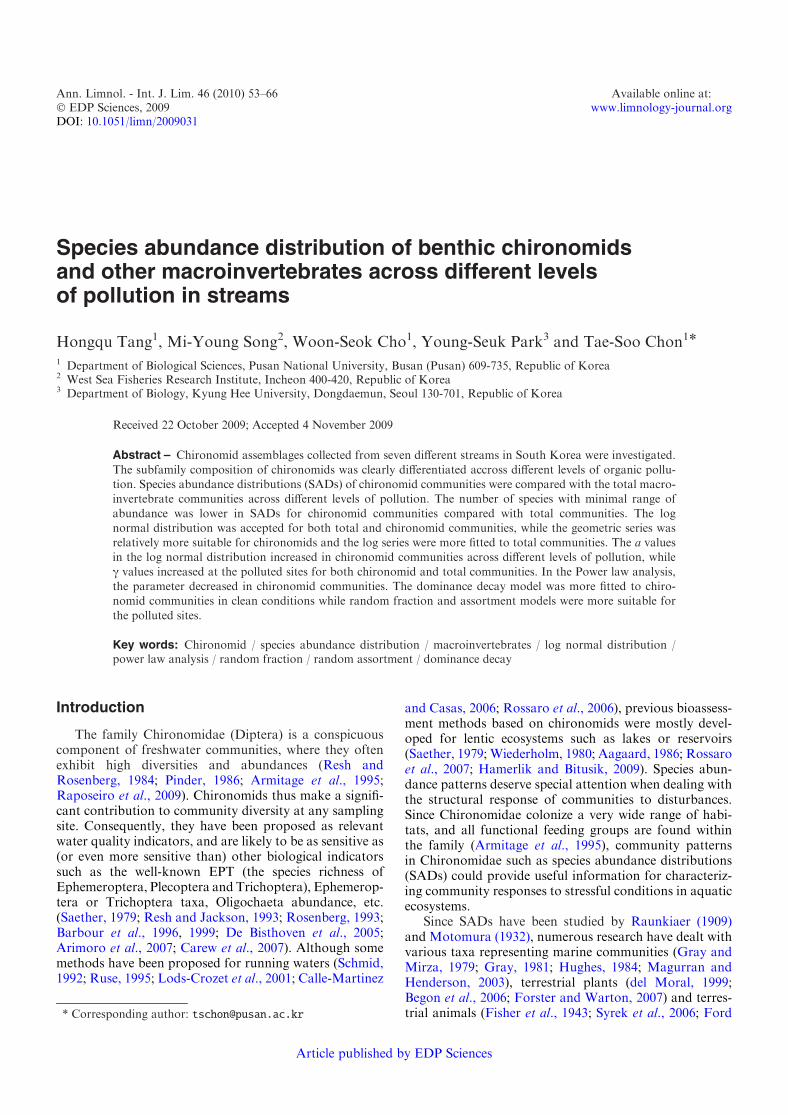
Species abundance distribution of benthic chironomids and other macroinvertebrates across different levels of pollution in streams Hongqu Tang 1 , Mi-Young Song 2 , Woon-Seok Cho 1 , Young-Seuk Park 3 and Tae-Soo Chon 1 * 1 Department of Biological Sciences, Pusan National University, Busan (Pusan) 609-735, Republic of Korea 2 West Sea Fisheries Research Institute, Incheon 400-420, Republic of Korea 3 Department of Biology, Kyung Hee University, Dongdaemun, Seoul 130-701, Republic of Korea Received 22 October 2009; Accepted 4 November 2009 Abstract – Chironomid assemblages collected from seven different streams in South Korea were investigated. The subfamily composition of chironomids was clearly differentiated accross different levels of organic pollu- tion. Species abundance distributions (SADs) of chironomid communities were compared with the total macro- invertebrate communities across different levels of pollution. The number of species with minimal range of abundance was lower in SADs for chironomid communities compared with total communities. The log normal distribution was accepted for both total and chironomid communities, while the geometric series was relatively more suitable for chironomids and the log series were more fitted to total communities. The a values in the log normal distribution increased in chironomid communities across different levels of pollution, while c values increased at the polluted sites for both chironomid and total communities. In the Power law analysis, the parameter decreased in chironomid communities. The dominance decay model was more fitted to chiro- nomid communities in clean conditions while random fraction and assortment models were more suitable for the polluted sites. Key words: Chironomid / species abundance distribution / macroinvertebrates / log normal distribution / power law analysis / random fraction / random assortment / dominance decay Introduction The family Chironomidae (Diptera) is a conspicuous component of freshwater communities, where they often exhibit high diversities and abundances (Resh and Rosenberg, 1984; Pinder, 1986; Armitage et al., 1995; Raposeiro et al., 2009). Chironomids thus make a signifi- cant contribution to community diversity at any sampling site. Consequently, they have been proposed as relevant water quality indicators, and are likely to be as sensitive as (or even more sensitive than) other biological indicators such as the well-known EPT (the species richness of Ephemeroptera, Plecoptera and Trichoptera), Ephemerop- tera or Trichoptera taxa, Oligochaeta abundance, etc. (Saether, 1979; Resh and Jackson, 1993; Rosenberg, 1993; Barbour et al., 1996, 1999; De Bisthoven et al., 2005; Arimoro et al., 2007; Carew et al., 2007). Although some methods have been proposed for running waters (Schmid, 1992; Ruse, 1995; Lods-Crozet et al., 2001; Calle-Martinez and Casas, 2006; Rossaro et al., 2006), previous bioassess- ment methods based on chironomids were mostly devel- oped for lentic ecosystems such as lakes or reservoirs (Saether, 1979; Wiederholm, 1980; Aagaard, 1986; Rossaro et al., 2007; Hamerlik and Bitusik, 2009). Species abun- dance patterns deserve special attention when dealing with the structural response of communities to disturbances. Since Chironomidae colonize a very wide range of habi- tats, and all functional feeding groups are found within the family (Armitage et al., 1995), community patterns in Chironomidae such as species abundance distributions (SADs) could provide useful information for characteriz- ing community responses to stressful conditions in aquatic ecosystems. Since SADs have been studied by Raunkiaer (1909) and Motomura (1932), numerous research have dealt with various taxa representing marine communities (Gray and Mirza, 1979; Gray, 1981; Hughes, 1984; Magurran and Henderson, 2003), terrestrial plants (del Moral, 1999; Begon et al., 2006; Forster and Warton, 2007) and terres- trial animals (Fisher et al., 1943; Syrek et al., 2006; Ford * Corresponding author: [email protected] Article published by EDP Sciences Ann. Limnol. - Int. J. Lim. 46 (2010) 53–66 Available online at: Ó EDP Sciences, 2009 www.limnology-journal.org DOI: 10.1051/limn/2009031
Transcript of Species abundance distribution of benthic chironomids and ... · PDF fileSpecies abundance...
Species abundance distribution of benthic chironomidsand other macroinvertebrates across different levelsof pollution in streams
Hongqu Tang1, Mi-Young Song2, Woon-Seok Cho1, Young-Seuk Park3 and Tae-Soo Chon1*
1 Department of Biological Sciences, Pusan National University, Busan (Pusan) 609-735, Republic of Korea2 West Sea Fisheries Research Institute, Incheon 400-420, Republic of Korea3 Department of Biology, Kyung Hee University, Dongdaemun, Seoul 130-701, Republic of Korea
Received 22 October 2009; Accepted 4 November 2009
Abstract – Chironomid assemblages collected from seven different streams in South Korea were investigated.
The subfamily composition of chironomids was clearly differentiated accross different levels of organic pollu-tion. Species abundance distributions (SADs) of chironomid communities were compared with the total macro-invertebrate communities across different levels of pollution. The number of species with minimal range of
abundance was lower in SADs for chironomid communities compared with total communities. The lognormal distribution was accepted for both total and chironomid communities, while the geometric series wasrelatively more suitable for chironomids and the log series were more fitted to total communities. The a valuesin the log normal distribution increased in chironomid communities across different levels of pollution, while
c values increased at the polluted sites for both chironomid and total communities. In the Power law analysis,the parameter decreased in chironomid communities. The dominance decay model was more fitted to chiro-nomid communities in clean conditions while random fraction and assortment models were more suitable for
the polluted sites.
Key words: Chironomid / species abundance distribution / macroinvertebrates / log normal distribution /power law analysis / random fraction / random assortment / dominance decay
Introduction
The family Chironomidae (Diptera) is a conspicuouscomponent of freshwater communities, where they oftenexhibit high diversities and abundances (Resh andRosenberg, 1984; Pinder, 1986; Armitage et al., 1995;Raposeiro et al., 2009). Chironomids thus make a signifi-cant contribution to community diversity at any samplingsite. Consequently, they have been proposed as relevantwater quality indicators, and are likely to be as sensitive as(or even more sensitive than) other biological indicatorssuch as the well-known EPT (the species richness ofEphemeroptera, Plecoptera and Trichoptera), Ephemerop-tera or Trichoptera taxa, Oligochaeta abundance, etc.(Saether, 1979; Resh and Jackson, 1993; Rosenberg, 1993;Barbour et al., 1996, 1999; De Bisthoven et al., 2005;Arimoro et al., 2007; Carew et al., 2007). Although somemethods have been proposed for running waters (Schmid,1992; Ruse, 1995; Lods-Crozet et al., 2001; Calle-Martinez
and Casas, 2006; Rossaro et al., 2006), previous bioassess-ment methods based on chironomids were mostly devel-oped for lentic ecosystems such as lakes or reservoirs(Saether, 1979; Wiederholm, 1980; Aagaard, 1986; Rossaroet al., 2007; Hamerlik and Bitusik, 2009). Species abun-dance patterns deserve special attention when dealing withthe structural response of communities to disturbances.Since Chironomidae colonize a very wide range of habi-tats, and all functional feeding groups are found withinthe family (Armitage et al., 1995), community patternsin Chironomidae such as species abundance distributions(SADs) could provide useful information for characteriz-ing community responses to stressful conditions in aquaticecosystems.
Since SADs have been studied by Raunkiaer (1909)and Motomura (1932), numerous research have dealt withvarious taxa representing marine communities (Gray andMirza, 1979; Gray, 1981; Hughes, 1984; Magurran andHenderson, 2003), terrestrial plants (del Moral, 1999;Begon et al., 2006; Forster and Warton, 2007) and terres-trial animals (Fisher et al., 1943; Syrek et al., 2006; Ford* Corresponding author: [email protected]
Article published by EDP Sciences
Ann. Limnol. - Int. J. Lim. 46 (2010) 53–66 Available online at:� EDP Sciences, 2009 www.limnology-journal.orgDOI: 10.1051/limn/2009031

and Lancaster, 2007). Extensive reviews can also be foundin May (1975), Tokeshi (1993), Magurran (2004), Mayet al. (2007), and McGill et al. (2007).
Regarding chironomid communities, various SADmodels have been proposed by Tokeshi (1990, 1993,1995, 1999), who reported that the random fraction andassortment models were successfully fitted to the chirono-mid communities based on individual data (Tokeshi,1990). Using chironomids collected from a large river,Fesl (2002) reported that the observed communities didnot fit the various niche-oriented models including thegeometric series, whereas the distribution of functionalfeeding groups in chironomids fitted the random fractionmodel. In contrast, Ruse (1995) found that the abundancepatterns of larval and pupal chironomids from a chalkstream were best described by a log series model. Alterna-tively, Dimitriadis and Cranston (2007) studied estuarialsystems, where abundance patterns of chironomid com-munities fitted geometric series. SADs were also checkedfor different life stages. Boerger (1981) collected emergingchironomids from a muskeg stream and reported therewere more rare species than expected from Preston’s log-normal distribution, while the community pattern, exclud-ing the rare species, did not differ significantly from the lognormal model.
Earlier studies on SADs in chironomids have con-sidered the impact of different stream types, coveringunpolluted (Schmid, 1992; Ruse, 1995), muskeg (Boerger,1981) and estuarial (Dimitriadis and Cranston, 2007)ecosystems. Previous research has been also carried outat sites under stressful conditions subjected to organicpollution (Calle-Martinez and Casas, 2006), or sedimentclogging (Carew et al., 2007) and river regulation (Penczaket al., 2006). However, these studies mostly aimed atdefining indicator groups for a selected range of distur-bances (Saether, 1975, 1979; Wiederholm, 1980; Rossaroet al., 2006). No extensive analysis has examined the SADsof chironomids in response to organic pollution, in com-parison with total benthic macroinvertebrates. Dimitriadisand Cranston (2007) recently checked the SADs ofChironomidae exposed to a salinity gradient, and reportedan overall satisfactory fit was achieved with the geometricseries. Recently, the SADs of total benthic macroinverte-brates in polluted streams were evaluated by Qu et al.(2008), who found that the SADs were useful for depictingthe ecological status of the sampling sites. As a continu-ation of this study, we investigated the SADs in chirono-mid communities and compared them with the structuralproperties of the total communities across different levelsof pollution.
Materials and methods
Study area
Data sets were built upon benthic macroinvertebratescollected at the 14 sampling sites in six streams (Mainchannel in the Nakdong River Basin, and streams of
Baenae, Daechon, Onchon, Hakjang, and Kumsan), in-cluding one large (Nakdong) and two short (Suyong andKumsan) river basins in Korea from 2004 to 2008 (Fig. 1,Table 1). The sampling sites represented different levelsof pollution (Table 1). An unpolluted site (B; BCN) wasselected from the Baenae Stream, a tributary located in themiddle course of the Nakdong River Basin. The Baenaestream is located in a mountainous area (Fig. 1) and isrelatively unpolluted (see Table 1). However, due to anincrease in summer tourism since the 1990’s there has beena corollary increase in the level of disturbance (Oh andChon, 1991a, 1991b, 1993).
The Keumsan stream (three successive sites; S1(KBK),S2(KMI), S3(KUP)) also located in a mountainous areawas additionally selected to represent unpolluted con-ditions (Fig. 1). The Onchon stream originates in a moun-tainous area and passes through a residential area (Kwaket al., 2002), thus presenting a range of unpolluted (O1;OCU) to polluted sites (O2; ONS) (Table 1). Since theearly 2000s, a recovery project has been conducted by thelocal government in this stream.
The Daechon Stream was selected to reflect the impactof different levels of organic pollution. It is a tributary ofNakdong River Basin that passes through a mountainousarea. The middle section of the stream has been heavilypolluted by the many restaurants in the area. Two sites(D2 (DDK) and D3 (DKS)) were polluted by domesticsewage (Song et al., 2005; Qu et al., 2008), while D1(DUK) was unpolluted in the upstream area. The site D4(DAG), located further downstream from D2 and D3(Fig. 1), showed a recovering status (see Table 1).
Two streams were selected to represent polluted andseverely polluted sites. Four sampling sites (N1 (NSJ), N2(NKJ), N3 (NJP), and N4 (NMK)) located in the mainstream of the Nakdong River Basin represented thepolluted state (Table 1). The sampling sites were locatedin the lower river basin in suburban area. Along with thesampling site in the Baenae Stream, the sample sites in themain channel of the Nakdong River have been surveyedfor the national LTER (Long-Term Ecological ResearchProject in Korea) since 2005.
The Hakjang Stream in the Nakdong River Basin is atributary of the Nakdong River Basin within Busan cityand was selected to represent severe pollution. The site K(HJD) in the Hakjang Stream has been heavily affected bydomestic and industrial pollution (see BOD and BMWPvalues in Table 1). The sampling procedure details weresummarized in Table 2. Seasonal samplings were carriedout from winter 2004 to spring 2007 in the Daechon andOnchon Streams, while monthly samplings were con-ducted at sites B, N1 and N2 from March 2005 to August2008. In total, 176 samples were analysed.
Community data
Benthic macroinvertebrates including chironomidswere collected using a Surber net (sampling area=30r30 cm2, mesh size=100 mm). Three collections mainly
H. Tang et al.: Ann. Limnol. - Int. J. Lim. 46 (2010) 53–6654

covering riffle zones were conducted as replicates at eachsite. Chironomid samples were sorted from the benthicmacroinvertebrates and preserved in 85% alcohol in thelaboratory. The larvae were further hand sorted under astereo-microscope and counted separately. For coarseidentification, sorted individuals were classified into sev-eral possible species groups based on similar morphologi-cal characters; such as body seta, body color, body shape,the location of eye, etc. Subsequently, at least 1–5 indi-viduals from each possible species groups were picked outand dissected into head and body to mount into slides byCMC-10 solution (Master Company, Inc., Illinois). Fineclassification was conducted under the compound micro-
scope by checking the mounted slides. In most cases thespecimens were identified to species or to the lowest pos-sible taxonomical level following the keys of Sasa (1979,1984), Ree and Kim (1981), Cranston (1982), Wiederholm(1983, 1986), Sasa and Kikuchi (1995), Epler (2001), Klinkand Moller Pillot (2003), Langton and Visser (2003),Wilson and Ruse (2005), Nittsuma and Yamamoto (2005)and Tang (2006). Part of the adult samples collected bysweep net or reared in the lab and the pupal samplescollected at the same place were further used to confirmthe larval status.
As many researchers have mentioned, classification ofall collected larvae is practically impossible (Kawai et al.,
Table 1. Environmental factors, Biological Monitoring Working Party (BMWP), and pollution states at the sample sites.
Streams Sites BOD (mg.Lx1) Turbidity (NTU) Conductivity (mS.cmx1) BMWP* Pollution levelBaenae B 1.15¡0.80 0.84¡0.95 23.86¡6.66 121 (68–157) LowKeumsan S1 2.23¡0.25 0.65¡0.39 31.79¡14.69 111 (87–131) Low
S2 3.41¡1.60 0.69¡0.70 48.06¡29.76 121 (96–162) LowS3 3.17¡0.51 1.11¡1.60 33.00¡20.37 111 (93–130) Low
Daechon D1 2.02¡2.34 5.54¡8.54 41.36¡7.66 110 (61–180) LowD2 6.88¡5.68 4.16¡3.97 176.76¡73.21 37 (17–52) IntermediateD3 4.52¡3.36 2.87¡2.31 211.90¡97.31 43 (15–76) IntermediateD4 2.56¡1.63 0.96¡0.78 161.03¡75.16 76 (44–116) Intermediate
Onchon O1 2.75¡1.70 2.43¡1.31 72.82¡43.29 128 (95–162) LowO2 3.78¡2.68 7.72¡10.41 237.51¡147.3 41 (24–54) Intermediate
Nakdong N1 9.84¡4.75 12.01¡10.28 311.95¡56.21 52 (20–75) HighN2 8.70¡5.49 10.90¡12.01 316.25¡64.73 40 (35–50) HighN3 7.38¡6.81 10.03¡6.21 452.25¡107.17 53 (30–82) HighN4 8.89¡6.64 17.61¡26.42 329.29¡120.78 26 (7–50) High
Hakjang K 31.80¡23.86 12.92¡9.03 480.44¡189.20 19 (9–36) Extreme
* Number in parenthesis is range.
Fig. 1. Location of sample sites in different streams in Korea.
H. Tang et al.: Ann. Limnol. - Int. J. Lim. 46 (2010) 53–66 55

1989; Rabeni and Wang, 2001), since there are numerousspecimens with small-sized individuals. Subsampling wasconducted if the number of individuals of some samplesexceeded 300, according to Barbour et al. (1999). In eachsubsample, 100–300 individuals were identified for thisstudy.
A biological index, the revised BMWP (Hawkes, 1997),was used to characterize the sites according to theidentified communities. Environmental variables were alsomeasured at each sampling time during the collection ofcommunities. Water temperature ( xC), dissolved oxygen(DO, mg.Lx1), conductivity (mS.cmx1), turbidity andother environmental factors were measured in situ withmultifunction probes. BOD5 was checked according toStandard Methods (APHA, AWWA and WPCF, 1985).
Data analysis – Species abundance distribution (SAD)
Considering that not all small chironomid larvae canbe identified, we chose models that are robust when deal-ing with missing rare species. In this regard the log normaldistribution (Preston, 1948; May, 1975) and the power law(Pueyo, 2006b) were used for analysis. The truncated lognormal distribution assumes that rare species are not fullysurveyed during the sampling, and the model would showa truncated pattern in the lower side of octaves in abun-dance (Preston, 1948; May, 1975; Magurran, 2004). Con-sequently, this model could be applicable when small andrare species are not extensively collected.
The log normal distribution (Preston, 1948; May, 1975)presents frequency of species arranged on the logarithmscale of species abundance in the normal distribution:
SðRÞ ¼ S0 expð�a2R2Þ ð3Þwhere S(R) is the number of species in the Rth octave (i.e.class) in abundance to the right and left of the symmetricalcurve and S0 is the number of species in the modal octave.Parameter a indicates the inverse width of the distribution:a= (2s2)x1/2 where s is the standard deviation of the
observed values after taking the logarithm (Preston, 1948;May, 1975). In this study, the truncated log normaldistribution was used to fit the community data based onMagurran (2004). After estimation of the parameters, theKolmogorov-Smirnov test (Sokal and Rohlf, 1995) wasused to check fitness of field data in the benthic inverte-brate communities (Qu et al., 2008).
The universality residing in the power law has beendemonstrated to reveal structural properties in thesampled communities. In the power law analysis, theslopes between species and log abundance could be rep-resented by excluding the maximal or minimal ranges inabundance (Pueyo, 2006b). The power law is based on thefollowing relationship (Pueyo, 2006a, 2006b):
pðnÞ/ n�b ð4Þwhere p(n) is the probability density of n individuals incommunities, and b is a constant. According to Pueyo(2006b), p(n) is replaced with f(n) as a continuum of prob-ability densities, and the value in each bin j was estimatedin our study as:
fðnjÞ ¼1
2jsjS
ð5Þ
where sj is the number of species in bin j for the abundanceclass (in this case, interval=2), 2j indicates the width ofbin j, and S is the total number of species. For eachbin j the (logarithmically) central value is nj ¼ 2jþ
12. The
maximum likelihood estimation was used to estimate theb values. The detailed method can be found in Pueyo(2006b) and Qu et al. (2008).
Two other traditional models widely used in analyzingSADs are the geometric and log series. We also checkedthe models for comparative purposes. In the geometricseries species abundance, ranked from most to leastabundant, is expressed as (Motomura, 1932; May, 1975;Magurran, 1988, 2004):
ni ¼ NCkð1� kÞi�1 ð1Þwhere ni is the number of individuals in the ith species, k isthe proportion of the available resource that each species
Table 2. Sampling methods and description of the sample areas.
Streams Sites Sampling frequency Sampling periods No. of samples AreaBaenae B Monthly May., 05–Aug., 08 31 MountainKeumsan S1 Seasonal Spr., 07–Aug., 08 7 Mountain
S2 Seasonal 7 MountainS3 Seasonal 7 Mountain
Daechon D1 Seasonal Win., 04–Spr., 07 11 Residence/MountainD2 Seasonal 11 Residence/MountainD3 Seasonal 11 Residence/MountainD4 Seasonal 11 Residence/Mountain
Onchon O1 Seasonal Win., 04–Spr., 07 11 MountainO2 Seasonal 11 Residence
Nakdong N1 Monthly Mar., 05–Aug.,08 14 SuburbanN2 Seasonal Spr., 05–Spr., 06 4 SuburbanN3 Seasonal Spr., 05–Spr., 06 4 SuburbanN4 Monthly Mar., 05–Mar., 08 25 Suburban
Hakjang K Seasonal Win., 04–Spr., 07 11 Industry
H. Tang et al.: Ann. Limnol. - Int. J. Lim. 46 (2010) 53–6656
utilizes, N is the total number of individuals, and Ck is aconstant ensuring
Pni ¼ N (see Magurran, 2004).
The log series originally proposed by Fisher et al.(1943) is presented as:
ax;ax2
2;ax3
3; . . . ;
axn
nð2Þ
where a is the index of diversity, n is species sequencefrom the minimum to the maximum, and x is estimatedfrom the iterative solution of S/N=(1xx)/x[x ln(1xx)](S, the total number of species, and N, the total number ofindividuals).
The SADmodels proposed for Chironomidae (Tokeshiand Townsend, 1987; Tokeshi, 1990) were also tested usingthe chironomids sampled in this study. The random frac-tion (RF) model was the basic concept for this type ofmodel, and various models were subsequently created toaccommodate diverse situations in niche preemption. Inthe RF model all species in an assemblage have the sameprobability of being selected for subsequent niche divisionby other invading species. The niche is first divided atrandom into two fractions, one of which is randomlychosen and divided at random into further two fractions.This type of fractioning continues to produce morefractions until niche space for the species with the lowestrank is formed (Tokeshi, 1990). The random assortmentmodel (RF) refers to a situation where abundances ofdifferent species are not mutually related. Niche space isrestricted in size only by its immediate, larger neighbor onthe niche-rank axis. This relationship can be expressed as:
Ni ¼ 1
Ni ¼ riNi�1 ði; integer greater than 1Þwhere Ni is the niche size (abundance) of rank i and riis an independent uniform random variable between 0and 1 (Tokeshi, 1990).
The dominance decay (DD) model refers to a situationwhere new species always take a portion of niche spacealready occupied by the most dominant species (Fesl,2002). Consequently the model is conducted toward thenegation of dominance and converges towards equitableabundances of constituent species (Tokeshi, 1990).
The RF, RA and DD models were applied to the fielddata. For fitting the models to the field data, 10 000 as-semblages were simulated in accordance with the numberof species collected in the field. The 95% confidence limits
were obtained from the simulation models and were usedfor checking the field data. The detailed method canbe found in Tokeshi (1990), Fesl (2002) and Magurran(2004).
Results
Composition of chironomid communities
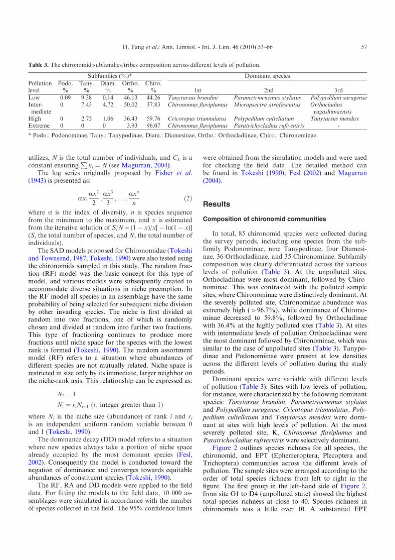
In total, 85 chironomid species were collected duringthe survey periods, including one species from the sub-family Podonominae, nine Tanypodinae, four Diamesi-nae, 36 Orthocladiinae, and 35 Chironominae. Subfamilycomposition was clearly differentiated across the variouslevels of pollution (Table 3). At the unpolluted sites,Orthocladiinae were most dominant, followed by Chiro-nominae. This was contrasted with the polluted samplesites, where Chironominae were distinctively dominant. Atthe severely polluted site, Chironominae abundance wasextremely high (>96.7%), while dominance of Chirono-minae decreased to 59.8%, followed by Orthocladinaewith 36.4% at the highly polluted sites (Table 3). At siteswith intermediate levels of pollution Orthocladiinae werethe most dominant followed by Chironominae, which wassimilar to the case of unpolluted sites (Table 3). Tanypo-dinae and Podonomiinae were present at low densitiesacross the different levels of pollution during the studyperiods.
Dominant species were variable with different levelsof pollution (Table 3). Sites with low levels of pollution,for instance, were characterized by the following dominantspecies: Tanytarsus brundini, Parametriocnemus stylatusand Polypedilum surugense. Cricotopus triannulatus, Poly-pedilum cultellatum and Tanytarsus mendax were domi-nant at sites with high levels of pollution. At the mostseverely polluted site, K, Chironomus flaviplumus andParatrichocladius rufiverntris were selectively dominant.
Figure 2 outlines species richness for all species, thechironomid, and EPT (Ephemeroptera, Plecoptera andTrichoptera) communities across the different levels ofpollution. The sample sites were arranged according to theorder of total species richness from left to right in thefigure. The first group in the left-hand side of Figure 2,from site O1 to D4 (unpolluted state) showed the highesttotal species richness at close to 40. Species richness inchironomids was a little over 10. A substantial EPT
Table 3. The chironomid subfamilies/tribes composition across different levels of pollution.
Pollutionlevel
Subfamilies (%)* Dominant species
Podo.%
Tany.%
Diam.%
Ortho.%
Chiro.% 1st 2nd 3rd
Low 0.09 9.38 0.14 46.13 44.26 Tanytarsus brundini Parametriocnemus stylatus Polypedilum surugenseInter-mediate
0 7.43 4.72 50.02 37.83 Chironomus flaviplumus Micropsectra atrofasciatus Orthocladiusyugashimaensis
High 0 2.75 1.06 36.43 59.76 Cricotopus triannulatus Polypedilum cultellatum Tanytarsus mendaxExtreme 0 0 0 3.93 96.07 Chironomus flaviplumus Paratrichocladius rufiventris -
* Podo.: Podonominae, Tany.: Tanypodinae, Diam.: Diamesinae, Ortho.: Orthocladiinae, Chiro.: Chironominae.
H. Tang et al.: Ann. Limnol. - Int. J. Lim. 46 (2010) 53–66 57
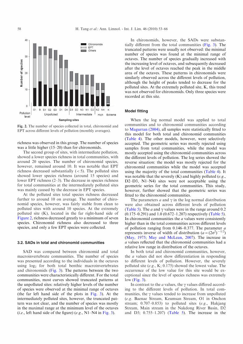
richness was observed in this group. The number of specieswas a little higher (15–20) than for chironomids.
The second group of sites, with intermediate pollution,showed a lower species richness in total communities, witharound 20 species. The number of chironomid species,however, remained around 10. It was notable that EPTrichness decreased substantially (<5). The polluted sitesshowed lower species richness (around 15 species) andlower EPT richness (2–3). The decrease in species richnessfor total communities at the intermediately polluted siteswas mainly caused by the decrease in EPT species.
At the polluted sites total species richness decreasedfurther to around 10 on average. The number of chiro-nomid species, however, was fairly stable from clean topolluted sites with around 10 species. At the extremelypolluted site (K), located in the far right-hand side ofFigure 2, richness decreased greatly to a minimum of sevenspecies. Chironomid richness also decreased to threespecies, and only a few EPT species were collected.
3.2. SADs in total and chironomid communities
SAD was compared between chironomid and totalmacroinvertebrate communities. The number of specieswas presented according to the individuals in the octavesusing log2 for both total benthic macroinvertebratesand chironomids (Fig. 3). The patterns between the twocommunities were characteristically different. For the totalcommunities, most curves showed truncated patterns atthe unpolluted sites: relatively higher levels of the numberof species were observed at the minimal range of octaves(the far left hand side of the plots in Fig. 3). At theintermediately polluted sites, however, the truncated pat-tern was not clear, and the number of species was mostlyin the maximal range at the minimum level of the octaves(i.e., left hand side of the figure) (e.g., N1–N4 in Fig. 3).
In chironomids, however, the SADs were substan-tially different from the total communities (Fig. 3). Thetruncated patterns were usually not observed: the minimalnumber of species was found at the minimal range ofoctaves. The number of species gradually increased withthe increasing level of octaves, and subsequently decreasedafter the level of octaves reached the peak in the middlearea of the octaves. These patterns in chironomids weresimilarly observed across the different levels of pollution,although the height of peaks tended to decrease for thepolluted sites. At the extremely polluted site, K, this trendwas not observed for chironomids. Only three species wererecorded at this site.
Model fitting
When the log normal model was applied to totalcommunities and to chironomid communities accordingto Magurran (2004), all samples were statistically fitted tothis model for both total and chironomid communities(Table 4). The other models, however, were selectivelyaccepted. The geometric series was mostly rejected usingsamples from total communities, while the model wasmostly accepted using the chironomid communities acrossthe different levels of pollution. The log series showed thereverse situation: the model was mostly rejected for thechironomid communities while the model was acceptedusing the majority of the total communities (Table 4). Itwas notable that the severely (K) and highly polluted (e.g.,D2–D3, N1–N4) sites were not acceptable using thegeometric series for the total communities. This study,however, further showed that the geometric series wasfitted to the chironomid communities.
The parameters a and c in the log normal distributionwere also obtained across different levels of pollution(Table 5). The a and c values were in the range around 0.2(0.175–0.291) and 1.0 (0.672–1.207) respectively (Table 5).In chironomid communities the a values were consistentlyhigher than in the total communities across different levelsof pollution ranging from 0.146–0.377. The parameter arepresents inverse of width of distribution (a= (2s2)x1/2)(May, 1975; May and McLean, 2007). The increase ina values reflected that the chironomid communities had arelative low range in distribution of the octaves.
In both total and chironomid communities, however,the a values did not show differentiation in respondingto different levels of pollution. However, the severelypolluted site (e.g., K; 0.175) showed the lowest value. Theoccurrence of the low value for this site would be ex-ceptional since the level of species richness was extremelylow (Fig. 3).
In contrast to the a values, the c values differed accord-ing to the different levels of pollution. In total com-munities, the c values tended to increase from unpolluted(e.g. Baenae Stream, Keumsan Stream, O1 in Onchonstream; 0.707–0.853) to polluted sites (e.g., HakjangStream, Main stream in the Nakdong River Basin, D2and D3; 0.755–1.207) (Table 5). The increase in the
Fig. 2. The number of species collected in total, chironomid and
EPT across different levels of pollution (monthly averages).
H. Tang et al.: Ann. Limnol. - Int. J. Lim. 46 (2010) 53–6658
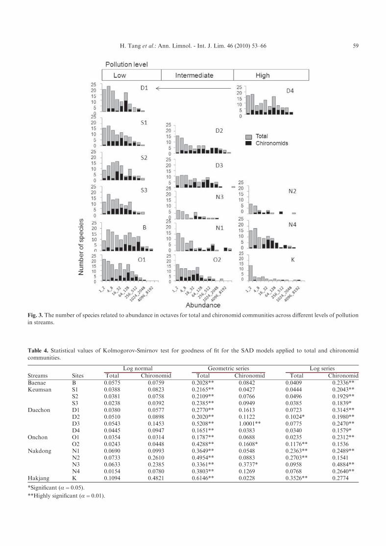
Fig. 3. The number of species related to abundance in octaves for total and chironomid communities across different levels of pollutionin streams.
Table 4. Statistical values of Kolmogorov-Smirnov test for goodness of fit for the SAD models applied to total and chironomidcommunities.
Streams Sites
Log normal Geometric series Log series
Total Chironomid Total Chironomid Total ChironomidBaenae B 0.0575 0.0759 0.2028** 0.0842 0.0409 0.2336**Keumsan S1 0.0388 0.0823 0.2165** 0.0427 0.0444 0.2043**
S2 0.0381 0.0758 0.2109** 0.0766 0.0496 0.1929**S3 0.0238 0.0392 0.2385** 0.0949 0.0385 0.1839*
Daechon D1 0.0380 0.0577 0.2770** 0.1613 0.0723 0.3145**D2 0.0510 0.0898 0.2020** 0.1122 0.1024* 0.1980**D3 0.0543 0.1453 0.5208** 1.0001** 0.0775 0.2470**D4 0.0445 0.0947 0.1651** 0.0383 0.0340 0.1579*
Onchon O1 0.0354 0.0314 0.1787** 0.0688 0.0235 0.2312**O2 0.0243 0.0448 0.4288** 0.1608* 0.1176** 0.1536
Nakdong N1 0.0690 0.0993 0.3649** 0.0548 0.2363** 0.2489**N2 0.0733 0.2610 0.4954** 0.0883 0.2703** 0.1541N3 0.0633 0.2385 0.3361** 0.3737* 0.0958 0.4884**N4 0.0154 0.0780 0.3803** 0.1269 0.0768 0.2640**
Hakjang K 0.1094 0.4821 0.6146** 0.0228 0.3526** 0.2774
*Significant (a=0.05).
**Highly significant (a=0.01).
H. Tang et al.: Ann. Limnol. - Int. J. Lim. 46 (2010) 53–66 59
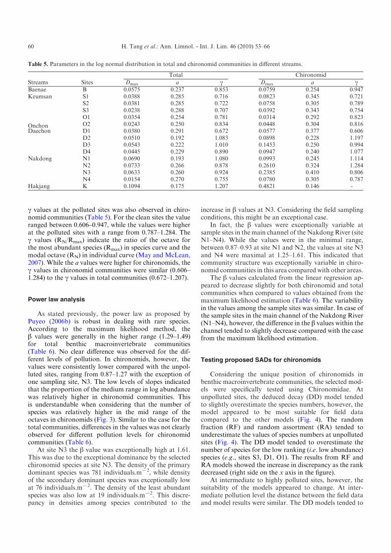
c values at the polluted sites was also observed in chiro-nomid communities (Table 5). For the clean sites the valueranged between 0.606–0.947, while the values were higherat the polluted sites with a range from 0.787–1.284. Thec values (RN/Rmax) indicate the ratio of the octave forthe most abundant species (Rmax) in species curve and themodal octave (RN) in individual curve (May and McLean,2007). While the a values were higher for chironomids, thec values in chironomid communities were similar (0.606–1.284) to the c values in total communities (0.672–1.207).
Power law analysis
As stated previously, the power law as proposed byPuyeo (2006b) is robust in dealing with rare species.According to the maximum likelihood method, theb values were generally in the higher range (1.29–1.49)for total benthic macroinvertebrate communities(Table 6). No clear difference was observed for the dif-ferent levels of pollution. In chironomids, however, thevalues were consistently lower compared with the unpol-luted sites, ranging from 0.87–1.27 with the exception ofone sampling site, N3. The low levels of slopes indicatedthat the proportion of the medium range in log abundancewas relatively higher in chironomid communities. Thisis understandable when considering that the number ofspecies was relatively higher in the mid range of theoctaves in chironomids (Fig. 3). Similar to the case for thetotal communities, differences in the values was not clearlyobserved for different pollution levels for chironomidcommunities (Table 6).
At site N3 the b value was exceptionally high at 1.61.This was due to the exceptional dominance by the selectedchironomid species at site N3. The density of the primarydominant species was 781 individuals.mx2, while densityof the secondary dominant species was exceptionally lowat 76 individuals.mx2. The density of the least abundantspecies was also low at 19 individuals.mx2. This discre-pancy in densities among species contributed to the
increase in b values at N3. Considering the field samplingconditions, this might be an exceptional case.
In fact, the b values were exceptionally variable atsample sites in the main channel of the Nakdong River (siteN1–N4). While the values were in the minimal range,between 0.87–0.93 at site N1 and N2, the values at site N3and N4 were maximal at 1.25–1.61. This indicated thatcommunity structure was exceptionally variable in chiro-nomid communities in this area compared with other areas.
The b values calculated from the linear regression ap-peared to decrease slightly for both chironomid and totalcommunities when compared to values obtained from themaximum likelihood estimation (Table 6). The variabilityin the values among the sample sites was similar. In case ofthe sample sites in the main channel of the Nakdong River(N1–N4), however, the difference in the b values within thechannel tended to slightly decrease compared with the casefrom the maximum likelihood estimation.
Testing proposed SADs for chironomids
Considering the unique position of chironomids inbenthic macroinvertebrate communities, the selected mod-els were specifically tested using Chironomidae. Atunpolluted sites, the deduced decay (DD) model tendedto slightly overestimate the species numbers, however, themodel appeared to be most suitable for field datacompared to the other models (Fig. 4). The randomfraction (RF) and random assortment (RA) tended tounderestimate the values of species numbers at unpollutedsites (Fig. 4). The DD model tended to overestimate thenumber of species for the low ranking (i.e. low abundance)species (e.g., sites S3, D1, O1). The results from RF andRA models showed the increase in discrepancy as the rankdecreased (right side on the x axis in the figure).
At intermediate to highly polluted sites, however, thesuitability of the models appeared to change. At inter-mediate pollution level the distance between the field dataand model results were similar. The DD models tended to
Table 5. Parameters in the log normal distribution in total and chironomid communities in different streams.
Streams Sites
Total Chironomid
Dmax a c Dmax a cBaenae B 0.0575 0.237 0.853 0.0759 0.254 0.947Keumsan S1 0.0388 0.285 0.716 0.0823 0.345 0.721
S2 0.0381 0.285 0.722 0.0758 0.305 0.789S3 0.0238 0.288 0.707 0.0392 0.343 0.754
Onchon
O1 0.0354 0.254 0.781 0.0314 0.292 0.823O2 0.0243 0.250 0.834 0.0448 0.304 0.816
Daechon D1 0.0380 0.291 0.672 0.0577 0.377 0.606D2 0.0510 0.192 1.083 0.0898 0.228 1.197D3 0.0543 0.222 1.010 0.1453 0.250 0.994D4 0.0445 0.229 0.890 0.0947 0.240 1.077
Nakdong N1 0.0690 0.193 1.080 0.0993 0.245 1.114N2 0.0733 0.266 0.878 0.2610 0.324 1.284N3 0.0633 0.260 0.924 0.2385 0.410 0.806N4 0.0154 0.270 0.755 0.0780 0.305 0.787
Hakjang K 0.1094 0.175 1.207 0.4821 0.146 -
H. Tang et al.: Ann. Limnol. - Int. J. Lim. 46 (2010) 53–6660

overestimate the species numbers, while the RF and RAmodels underestimated the value similar to what is shownin the DD model results. For the RF and RA models,however, one case matched well to field data (i.e., site O2),while the DD model still overestimated at this sample site(Fig. 4).
At highly polluted sites, the RF and RA modelsappeared to be more suitable for the field data than theDD model. While the DD model still overestimated thenumber of species at most sample sites, the RF and RAmodels were closer to the field data as shown at site N2(Fig. 4). At site N4, however, results from all models didnot agree with the field data. At the severely polluted site,K, the three models were similar with each slightly over-estimating the number of individuals of the secondarydominant species. The number of species was exception-ally low in this case, and results may need confirmationfrom more sample sites in similar conditions (Fig. 4). Therelative abundance obtained from the RF and RA modelswere similar across the different levels of pollution.
Discussion
Our results demonstrated that SADs as applied to bothtotal macroinvertebrates and chironomids could efficientlyreveal structural changes in communities in responseto disturbance. The distinctive appearance of dominantspecies (Table 3) was in accordance with previous studiesdefining the indicator groups as they relate to the differenthabitat conditions (Saether, 1979; Wiederholm, 1980;Hellawell, 1986; Calle-Martinez and Casas, 2006;Penczak et al., 2006; Rossaro et al., 2006; Carew et al.,2007). For both total and chironomid communities the lognormal model appeared most suitable. Although thismodel would not identify the dynamic processes in com-munity development, the model was confirmed again tobe widely fitted to field data (Diserud and Engen, 1999;Magurran, 2004; May et al., 2007).
In the study of chironomids, identification of all speci-mens is a problematic issue. The collection of chironomidsrequired a dense mesh 100–200 mm in size and numeroussmall-sized individuals are frequently collected, while miss-ing some small individuals is unavoidable (Storey andPinder, 1985; Tokeshi, 1995). Although chironomid larvaeplay an important role in the benthic fauna, taxonomicdifficulty often forces the investigators to treat them athigher levels, most often covering the (sub)-family or tribe(Armitage and Blackburn, 1985; Hilsenhoff, 1988), genus(Balloch et al., 1976; Warwick, 1993), or uncertain classi-fied species (Kwon and Chon, 1991; Youn and Chon,1999).
Since application of the truncated log normal dis-tribution assumes insufficient sampling of rare species, themodel was suitable for checking the SADs in chironomids.Overall fitting to log normal distribution in total com-munities and the selected acceptance with the geometricand log series were generally in accordance with resultsfrom Qu et al. (2008).T
able6.Statisticsofpower
lawanalysisapplied
toSAD
modelsin
totalandchironomid
communitiesin
differentstreams.
Streams
Sites
Total
Chironomids
ExcludingChironomids
NS
Maxim
um
likelihood
estimation
Linear
regression
NS
Maxim
um
likelihood
estimation
Linear
regression
NS
Maxim
um
likelihood
estimation
Linear
regression
b95%
C.I.*
bR2
b95%
C.I.
bR2
b95%
C.I.
bR2
Baenae
B23179
135
1.29
1.17–1.40
1.21
0.98
12437
40
1.09
0.85–1.33
0.95
0.92
10742
95
1.36
1.18–1.53
1.33
0.97
Keumsan
S1
4039
95
1.46
1.35–1.56
1.39
0.98
1413
30
1.23
0.92–1.53
1.05
0.9
2626
65
1.50
1.39–1.60
1.43
0.98
S2
5442
92
1.37
1.22–1.52
1.28
0.97
2082
34
1.17
0.89–1.44
1.01
0.94
3360
58
1.44
1.25–1.63
1.33
0.95
S3
4172
91
1.37
1.23–1.52
1.34
0.98
1500
32
1.23
0.91–1.54
1.04
0.89
2672
59
1.47
1.33–1.62
1.39
0.97
Onchon
O1
9539
130
1.41
1.29–1.52
1.34
0.97
4984
32
1.16
0.89–1.43
0.97
0.90
4555
98
1.42
1.33–1.52
1.36
0.99
O2
10282
88
1.37
1.28–1.47
1.31
0.99
2566
32
1.27
1.02–1.52
1.10
0.93
7716
56
1.40
1.29–1.52
1.33
0.98
Daechon
D1
4231
114
1.49
1.38–1.61
1.43
0.98
1359
26
1.14
0.62–1.66
1.00
0.84
2872
88
1.55
1.45–1.64
1.49
0.99
D2
26504
84
1.30
1.22–1.38
1.23
0.99
13963
36
1.05
0.85–1.25
0.95
0.95
12541
48
1.33
1.23–1.43
1.24
0.97
D3
25252
79
1.32
1.23–1.42
1.26
0.98
6967
33
1.14
0.91–1.37
1.00
0.92
18285
46
1.32
1.24–1.40
1.28
0.99
D4
14092
111
1.30
1.17–1.42
1.21
0.98
7920
36
1.04
0.82–1.25
0.97
0.95
6172
75
1.34
1.17–1.50
1.26
0.99
Nakdong
N1
22886
65
1.33
1.18–1.48
1.23
0.96
15269
18
0.98
0.78–1.18
0.93
0.94
7617
47
1.47
1.31–1.63
1.37
0.97
N2
1488
27
1.39
1.17–1.60
1.28
0.96
353
80.87
0.52–1.23
0.87
0.95
1135
19
1.39
1.07–1.71
1.28
0.95
N3
1830
33
1.44
1.29–1.60
1.33
0.97
994
71.61
0.98–2.24
1.30
0.98
836
26
1.48
1.30–1.65
1.39
0.97
N4
5137
85
1.47
1.37–1.58
1.41
0.98
4234
34
1.25
1.02–1.48
1.10
0.91
903
51
1.56
1.44–1.69
1.49
0.99
Hakjang
K77923
37
1.37
1.25–1.48
1.27
0.98
7197
30.93
0.61–1.25
1.00
1.00
70726
34
1.39
1.24–1.54
1.29
0.98
*95%
confidence
interval.
H. Tang et al.: Ann. Limnol. - Int. J. Lim. 46 (2010) 53–66 61

This study also showed that the parameters in the lognormal distribution would present the structural differ-ences in communities responding to pollution. Thec values in the log normal model tended to increase forpolluted sites in both total and chironomid communities.The increase in c values implied that the tolerant specieswere selectively adapted to polluted conditions and be-came increasingly dominant. Consequently, the tendencyfor dominancy would be stronger at polluted sites as in-crease in the c values suggested.
The structural difference between the total benthicmacroinvertebrates and chironomid communities in therichness-abundance (in octave) relationships may haveoriginated from sample collection issues (Fig. 3). Thespecies numberwas characteristically high for the lowabun-dance in the total communities. In total communities, thereare numerous taxa besides Chironomidae, and there would
be a higher chance of rare species being present. Driftingwould be a source of rare species in streams. Trichoptera,especially Hydropsychidae, were most frequently collectedin small numbers (1–2 individuals) over a broad range atunpolluted sites. Ephemeroptera, including Ephemeridaeand Ephemerellidae, were also often observed at the inter-mediately and highly polluted sites in minimal numbers.Considering that these species in Ephemeroptera andTrichoptera are usually found in unpolluted areas, thespecies may have drifted down from upstream and couldcontribute to the increase in number of species with lownumbers in total communities (Fig. 3). At polluted sites,the species from upstream were also found in low abun-dance including 1–2 rare species from the Ephemeroptera,Diptera and Trichoptera. Besides insect species, species inHirudinea were also widely collected in minimal numbersfrom intermediate to extremely polluted sites.
Fig. 4. Comparison of SAD models applied to abundance (normalized) in relation to the rank of species in chironomid communities
across different levels of pollution in streams. Low, intermediate, and high and severe levels in pollution (vertical bars shown with themodel curves indicating 95% confidence intervals).
H. Tang et al.: Ann. Limnol. - Int. J. Lim. 46 (2010) 53–6662

In this study, b values in the Power analysis were nothighly variable between the different levels of pollution. InQu et al. (2008), the b values increased at recovering sites.The parameters were measured at one site at different timesin this case, reflecting the recovery of water quality. In thisstudy, however, this type of parameter change was notobserved. The b values may be variable depending uponthe diversity of habitat conditions at sample sites. Moreconsideration is needed to check community response andthe scale free structure in communities in the future.
The change in suitability of the DD, RF and RAmodels to different levels of pollution was also noticeable.While the DD model was more fitted to unpolluted sites,the RF and RA models tended to be more suitable forpolluted sites (Fig. 4). This indicated that random effectswould play an important role in disturbing conditions.Tokeshi (1987) also mentioned that random effects wouldcontribute greatly in determining species abundance ofchironomids. At site site N4 (also highly polluted),however, all the models did not fit the field data (Fig. 4).Communities collected at N4 were exceptional. Somespecies with the lower modal octave in individual curveswere more frequently collected and consequently theoctave for RN was lower than the octave for Rmax: abouteight species with lower octave (17–32 individuals.mx2)including Chironomus flaviplumus, Cryptochironomus ros-tratus and Tanytarsus mendax were abundantly collectedat N4. In this case Rmax usually belonging to the octavewas 33–64 individuals.mx2. This contributed to a decreasein the c values (Table 5), indicating that some speciesranked at low–intermediate levels were abundantly col-lected. This type of species distribution was not suitablefor applying the proposed SAD models for chironomids.
TheDDmodel, however, was useful at unpolluted sites.In this case the degree of niche preemption may be notstrong since the DD model supports negation of domi-nance (Tokeshi, 1990). This indicated that dominancy wasunfavorable and niche division occurred for the mostdominant species. Futher research is required in checkinghow the subdivision pattern of niche will occur in aquaticconditions in this study. In fact, a wide variety of SADmodels have been proposed including random fraction orassortment (Tokeshi, 1990, 1993, 1999; Fesl, 2002), logseries (Ruse, 1995), geometric series (Dimitriadis andCranston, 2007). This indicated that chironomid com-munites would show diverse SAD patterns in adapting tocompetition for resources and for environmental distur-bances at study sites. Our study confirmed a wide variety inSADs, including the DD model adaptable to unpollutedsites. The mechanism of niche sharing among the residingspecies, however, needs to be further considered.
Conclusions
Comparative studies on SADs between total macro-invertebrates and chironomids were useful in revealingstructural properties in communities responding to dis-turbance. The number of rare species was relatively higher
in total communities, while the number of rare species waslow and gradually increased to peak in the middle rangesof octaves in chironomid communities. Both total andchironomid communities were fitted to the log normal dis-tribution, and the change in parameter (c) would be usefulfor community structure in diagnosing polluted sites.When the models proposed for chironomids were tested,the most suitable model was the DD model for clean con-ditions. The suitability changed to RF and RA models forpolluted sites, indicating an increase in randomness ofcommunity establishment in disturbed conditions. Com-parative studies of SADs in chironomids and macroinvert-brates would provide significant insight into changes incommunity structure and ecological assessment of waterquality.
Acknowledgements. This study was financially supported byPusan National University in the program, “Post-Doc. 2008”.
This work was supported by the Korea Research FoundationGrant funded by the Korean Government (MOEHRD) (KRF-2007-313-C00748).
The first author is also indebted to Professor Ole A. Saether,
Bergen Museum, Bergen University, for providing hundredsof chironomids taxonomy references, special thanks to theDr. Les Ruse, the Environment Agency, Reading, UK, for his
encouragements and for providing us with many of his publi-cations. Many thanks to two Japanese colleagues, Dr. HiromiNiitsuma of Shizuoka University and Dr. Tadashi Kobayashi
of Kanagawa Prefecture for confirming several Tanypodinaespecies.
References
Aagaard K., 1986. The chironomid fauna of North Norwegianlakes, with a discussion on methods of community classifica-tion. Holarctic Ecol., 9, 1–12.
APHA, AWWA and WPCF, 1985. Standard methods for theexamination of water and waste, 16th edn., American publichealth association, Washington, 1268 p.
Arimoro F.O., Ikomi R.B. and Iwegbue C.M.A., 2007. Waterquality changes in relation to Diptera community patternsand diversity measured at an organic effluent impactedstream in the Niger Delta, Nigeria. Ecol. Indic., 7, 541–552.
Armitage P.D. and Blackburn J.H., 1985. Chironomidae in aPennine stream system receiving mine drainage and organicenrichment. Hydrobiologia, 121, 165–172.
Armitage P.D., Cranston P.S. and Pinder L.C.V. (eds.), 1995.The Chironomidae. The biology and ecology of non-bitingmidges, Chapman & Hall, London, 572 p.
Balloch D., Davies C.E. and Jones F.H., 1976. Biologicalassessment of water quality in three British rivers: the NorthEsk (Scotland), the Ivel (England) and the Taf (Wales).Water Pollut. Control, 75, 92–114.
Barbour M.T., Gerritsen J., Griffith G.E., Frydenborg R.,McCarron E., White J.S. and Bastian M.L., 1996. A frame-work for biological criteria for Florida streams using benthicmacroinvertebrates. J. N. Amer. Benthol. Soc., 15, 185–211.
BarbourM.T., Gerritsen J., Snyder B.D. and Stribling J.B., 1999.Rapid bioassessment protocols for use in streams and
H. Tang et al.: Ann. Limnol. - Int. J. Lim. 46 (2010) 53–66 63

wadeable rivers: periphyton, benthic macroinvertebrates andfish, 2nd edn., EPA 841-B-99-002, U.S. EnvironmentalProtection Agency, Office of Water, Washington, D.C.
Begon M., Townsend C.R. and Harper J.L., 2006. Ecology:from individuals to ecosystems, 4th edn., Blackwell, Malden,738 p.
Boerger H., 1981. Species composition, abundance and emer-gence phenology of midges in a brown-water stream of West-Central Alberta, Canada. Hydrobiologia, 80, 7–30.
Calle-Martinez D. and Casas J.J., 2006. Chironomid species,stream classification, and water-quality assessment: the caseof 2 Iberian Mediterranean mountain regions. J. N. Am.Benthol. Soc., 25, 465–476.
Carew M.E., Pettigrove V., Cox R.L. and Hoffmann A.A., 2007.The response of Chironomidae to sediment pollutionand other environmental characteristics in urban wetlands.Freshwat. Biol., 52, 2444–2462.
Cranston P.S., 1982. A key to the larvae of the BritishOrthocladiinae (Chironomidae). Scientific Publications ofFBA, 45, 1–152.
De Bisthoven L.J., Gerhardt A. and Soares A.M.V.A., 2005.Chironomid larvae as bioindicators of an acid mine drainagein Portugal. Hydrobiologia, 532, 181–191.
Del Moral R., 1999. Plant succession on pumice at MountSt. Helens, Washington. Am. Mid. Nat., 141, 101–114.
Dimitriadis S. and Cranston P.S., 2007. From the mountains tothe sea: assemblage structure and dynamics in Chironomidae(Insecta: Diptera) in the Clyde River estuary gradient,New South Wales, southeastern Australia. Aust. J. Entomol.,46, 188–197.
Diserud O.H. and Engen S., 1999. A general and dynamic speciesabundance model, embracing the lognormal and the Gammamodels. Am. Nat., 155, 498–511.
Epler J.H., 2001. Identification Manual for the LarvalChironomidae (Diptera) of North and South Carolina –A guide to the taxonomy of the midges of the southeasternUnited States, including Florida, North Carolina Depart-ment of Environment and Natural Resources, Raleigh, NC,and St. Johns River Water Management District, Palatka.
Fesl C., 2002. Niche-oriented species-abundance models: differ-ent approaches of their application to larval chironomid(Diptera) assemblages in a large river. J. Anim. Ecol., 71,1085–1094.
Fisher R.A., Corbet A.S. and Williams C.B., 1943. The relationbetween the number of species and the number of individualsin a random sample of an animal population. J. Anim. Ecol.,12, 42–58.
Ford N.B. and Lancaster D.L., 2007. The species-abundancedistribution of snakes in a bottomland hardwood forest ofthe southern United States. J. Herpetology, 41, 385–393.
Forster M.A. and Warton D.I., 2007. A metacommunity-scalecomparison of species-abundance distribution models forplant communities of eastern Australia. Ecography, 30,449–458.
Gray J.S., 1981. Detecting pollution induced changes in commu-nities using the log-normal distribution of individuals amongspecies. Mar. Pollut. Bull., 25, 48–50.
Gray J.S. and Mirza F.B., 1979. A possible method for thedetection of pollution-induced disturbance on marine benthiccommunities. Mar. Pollut. Bull., 10, 142–146.
Hamerlik L. and Bitusik P., 2009. The distribution of littoralchironomids along an altitudinal gradient in High Tatra
Mountain lakes: could they be used as indicators of climatechange? Ann. Limnol. - Int. J. Lim., 45, 145–156.
Hawkes H.A., 1997. Origin and Development of the BiologicalMonitoring Working Party Score System. Water Res., 32,964–968.
Hellawell J.M., 1986. Biological indicators of freshwater pollu-tion and environmental management, Elsevier, Amsterdam,446 p.
Hilsenhoff W.L., 1988. Rapid field assessment of organicpollution with a family-level biotic index. J. N. Am. Benthol.Soc., 7, 65–68.
Hughes R.G., 1984. A model of the structure and dynamics ofbenthic marine invertebrate communities. Mar. Ecol. Progr.,15, 1–11.
Kawai K., Yamagishi T. and Kubo Y., 1989. Usefulness ofchironomid larvae as indicators of water quality. Jpn. J.Sanitation. Zool., 40, 4, 269–283.
Klink A.G. and Moller Pillot H.K.M., 2003. Chironomidaelarvae – Key to the higher taxa and species of the lowlandsof Northwestern Europe, World Biodiversity DatabaseCD-ROM series, ETI, Amsterdam.
Kwak I.-S., Liu G.C., Park Y.-S., Song M.-Y. and Chon T.-S.,2002. Characterization of benthic macroinvertebrate com-munites and hydraulic factors in small-scale habitats in apolluted stream. Korean J. Limnol., 35, 295–305.
Kwon T.-S. and Chon T.-S., 1991. Ecological studies on benthicmacroinvertebrates in the Suyong River – II. Investigationson distribution and abundance in its main stream and fourtributaries. Korean J. Limnol., 24, 179–198.
Langton P.H. and Visser H., 2003. Chironomidae exuviae –A key to pupal exuviae of the West Palaearctic Region,Biodiversity Center of ETI, Amsterdam, CD-ROM.
Lods-Crozet B., Vencioni V., Olafsson J.S., Snook D.L.,Velle G., Brittain J.E., Castella E. and Rossaro B., 2001.Chironomid (Diptera: Chironomidae) communities in sixEuropean glacier-fed streams. Freshwat. Biol., 46, 1791–1809.
Magurran A.E., 1988. Ecological diversity and its measurement.Chapman & Hall, London, 179 p.
Magurran A.E., 2004. Measuring biological diversity, Blackwell,Oxford, 256 p.
Magurran A.E. and Henderson P.A., 2003. Explaining the excessof rare species in natural species abundance distributions.Nature, 422, 714–716.
May R.M., 1975. Patterns of species abundance and diversity. In:Cody M. and Diamond J.M. (eds.), Ecology of species andcommunities, Harvard University Press, Cambridge, 81–120.
May R.M. and McLean A.R. (eds.), 2007. Theoretical ecology:Principles and applications, Oxford University Press,Oxford, 257 p.
May R.M., Crawley M.J. and Sugihara G., 2007. Communities:patterns. In: May R.M. and McLean A.R. (eds.), Theoreticalecology: principles and applications, Oxford UniversityPress, Oxford, 111–131.
McGill B.J., Etienne R.S., Gray J.S., Alonso D., Anderson M.J.,Benecha H.K., Dornelas M., Enquist B.J., Green J.L., HeF.L., Hurlbert A.H., Magurran A.E., Marquet P.A., MaurerB.A., Ostling A., Soykan C.U., Ugland K.I. and White E.P.,2007. Species abundance distribution: moving beyond singleprediction theories to integration within an ecological frame-work. Ecol. Lett., 10, 995–1015.
Motomura I., 1932. On the statistical treatment of communities.Zool. Manage., Tokyo, 44, 379–383.
H. Tang et al.: Ann. Limnol. - Int. J. Lim. 46 (2010) 53–6664

Niitsuma H. and Yamamoto M., 2005. Chironomidae. In: KwaiT. and Tanida K. (eds.), Aquatic insects of Japan: Manualwith keys and illustrations, Tokai University Press,Kanagawa, 1035–1185.
Oh Y.-N. and Chon T.-S., 1991a. A study on the benthicmacroinvertebrates in the middle reaches of the Paenaestream, a tributary of the Nakdong River, Korea. I.Community analysis and biological assessment of the waterquality. Korean J. Ecol., 14, 345–360.
Oh Y.-N. and Chon T.-S., 1991b. A study on the benthicmacroinvertebrates in the middle reaches of Paenae stream, atributary of the Naktong River, Korea. II. Comparison ofcommunities and environments at the upper and lower sitesof levees. Korean J. Ecol., 14, 399–413.
Oh Y.-N. and Chon T.-S., 1993. A study on the benthicmacroinvertebrates in the middle reaches of Paenae stream,a tributary of the Naktong River, Korea III. Drifting aquaticinsects in four seasons. Korean J. Ecol., 16, 489–499.
Penczak T., Kruk A., Grzybkowska M. and Dukowsaka M.,2006. Patterning of impoundment impact of chironomidassemblages and their environment with use of the self-organizing map (SOM). Acta Oecol., 30, 312–321.
Pinder L.C.V., 1986. Biology of freshwater Chironomidae. Annu.Rev. Entomol., 31, 1–23.
Preston F.W., 1948. The commonness and rarity of species.Ecology, 29, 254–283.
Pueyo S., 2006a. Self-similarity in species-area relationship andin species abundance distribution. Oikos, 112, 156–162.
Pueyo S., 2006b. Diversity: between neutrality and structure.Oikos, 112, 392–405.
Qu X.D., Song M.-Y., Park Y.-S., Oh Y.-N. and Chon T.-S.,2008. Species abundance patterns of benthic macroinverte-brate communities in polluted streams. Ann. Limnol. - Int. J.Lim., 44, 119–133.
Rabeni C. and Wang N., 2001. Bioassessment of streams usingmacroinvertebrates: Are the Chironomidae necessary?Environ. Monit. Assess., 71, 177–185.
Raunkiaer C., 1909. Formationsundersogelse og Formations-statistik. Botanisk Tidskrift, 30, 20–132.
Raposeiro P.M., Hughes S.J. and Costa A.C., 2009. Chirono-midae (Diptera: Insecta) in oceanic islands: New records forthe Azores and biogeographic notes. Ann. Limnol. - Int. J.Lim., 45, 59–67.
Ree H.I. and Kim H.S., 1981. Studies on Chironomidae(Diptera) in Korea. I. Taxonomical study on adults ofChironomidae. Proc. Coll. Nat. Sci., SNU, 6, 123–226.
Resh V.H. and Jackson J.K., 1993. Rapid assessment approachesto biomonitoring using benthic macroinvertebrates. In:Rosenberg D.M. and Resh V.H. (eds.), Freshwater bio-monitoring in benthic macroinvertebrates, Chapman & Hall,New York, 195–233.
Resh V.H. and Rosenberg D.M. (eds.), 1984. The ecology ofaquatic insects, Praeger, New York, 625 p.
Rosenberg D.M., 1993. Freshwater biomonitoring and Chirono-midae. Neth. J. Aquat. Ecol., 26, 101–122.
Rossaro B., Lencioni V., Boggero A. and Marziali L., 2006.Chironomids from Southern Alpine running waters: ecology,biogeography. Hydrobiologia, 562, 231–246.
Rossaro B., Marziali L., Cardoso A.C., Solimini A., Free G. andGiacchini R., 2007. A biotic index using benthic macro-invertebrates from Italian lakes. Ecol. Indic., 7, 412–429.
Ruse L.P., 1995. Chironomid community structure deducedfrom larvae and pupal exuviae of a chalk stream. Hydro-biologia, 315, 135–142.
Saether O.A., 1975. Nearctic chironomids as indicators of laketypology. Verhangen Int. Verein Limnol., 19, 3127–3133.
Saether O.A., 1979. Chironomid communities as water qualityindicators. Holarctic Ecol., 2, 65–74.
Sasa M., 1979. A morphological study of adults and immaturestages of 20 Japanese species of the family Chironomidae(Diptera). Research Report of NIES, 7, 1–148.
Sasa M., 1984. Studies on chironomid midges in lakes of theNikko National Park. Pt. II. Taxonomical and morphologi-cal studies on the chironomid species collected from lakesin the Nikko National Park. Research Report of NIES, 70,16–215.
Sasa M. and Kikuchi M., 1995. Chironomidae (Diptera) fromJapan, University of Tokyo Press, Tokyo, 333 p.
Schmid P.E., 1992. Community structure of larval Chironomidaein a backwater area of the River Danube. Freshw. Biol., 27,151–167.
Sokal R.R. and Rohlf F.J., 1995. Biometry: the principlesand practice of statistics in biological research, 3rd edn.,W.H. Freeman and Company, New York, 887 p.
Song M.-Y., Lee S.-E., Park J.-I., Kim B.-H., Koh S.-C., LeeK.-S., Park Y.-S. and Chon T.-S., 2005. Comparative com-munity analysis of benthic macroinvertebrates and micro-organisms across different levels of organic pollution in astream by using artificial neural networks. WSEAS Trans.Biol. Biomed., 3, 257–268.
Storey A.W. and Pinder L.C.V., 1985. Mesh-size efficiency ofsampling of larval Chironomidae. Hydrobiologia, 124, 193–197.
Syrek D., Weiner W.M., Wojtylak M., Olszowska G.Y. andKwapis Z., 2006. Species abundance distribution of collem-bolan communities in forest soils polluted with heavy metals.Appl. Soil Ecol., 31, 239–250.
Tang H.Q., 2006. Biosystematic study on the chironomid larvaein China (Diptera, Chironomidae), Ph.D. Thesis, NankaiUniversity, 945 p.
Tokeshi M., 1990. Niche apportionment or random assortment:species abundance patterns revisited. J. Anim. Ecol., 59,1129–1146.
Tokeshi M., 1993. Species abundance patterns and communitystructure. Adv. Ecol. Res., 24, 111–186.
Tokeshi M., 1995. Species interactions and community structure.In: Armitage P.D., Cranston P.S. and Pinder L.C.V. (eds.),The Chironomidae: biology and ecology of non-bitingmidges, Chapman & Hall, London, 297–335.
Tokeshi M., 1999. Species Coexistence: Ecological andEvolutionary Perspectives, Blackwell Science, Oxford, 454 p.
Tokeshi M. and Townsend C.R., 1987. Random patch formationand weak competition: coexistence in an epiphytic chirono-mid community. J. Anim. Ecol., 56, 833–845.
Warwick W.F., 1993. The effect of trophic/contaminant inter-actions on Chironomid community structure and succession(Diptera, Chironomidae). Neth. J. Aquat. Ecol., 26, 563–575.
Wiederholm T., 1980. Use of benthos in lake monitoring.J. Water Poll. Control Federation, 52, 537–547.
Wiederholm T. (ed.), 1983. Chironomidae of the Holarcticregion. Keys and Diagnoses. Part 1. Larvae. Entomol.Scand. Suppl., 19, 1–457.
H. Tang et al.: Ann. Limnol. - Int. J. Lim. 46 (2010) 53–66 65

Wiederholm T. (ed.), 1986. Chironomidae of the Holarcticregion. Keys and Diagnoses. Part II. Pupae. Entomol.Scand. Suppl., 28, 1–482.
Wilson R.S. and Ruse L.P., 2005. A guide to the identificationof genera of chironomid pupal exuviae occurring in Britainand Ireland (including common genera from NorthernEurope) and their use in monitoring lotic and lentic
freshwater, Freshwater Biological Association, Special Pub-lication, No. 13, The Ferry House, Far Sawrey, Ambleside,Cumbria.
Youn B.-J. and Chon T.-S., 1999. Effects of the pollution oncommunities of Chironomidae (Diptera) in the SoktaeStream a tributary of the Suyong River. Korean J. Limnol.,32, 24–34.
H. Tang et al.: Ann. Limnol. - Int. J. Lim. 46 (2010) 53–6666