Special Studies for TxDOT Administration in FY...

Technical Report Documentation . Report No.

FHWA/TX-10/0-6581-CT-1 2. Government Accession No.

3. Recipient’s Catalog No.

4. Title and Subtitle Special Studies for TxDOT Administration in FY 2009

5. Report Date October 2009; Revised December 2009

6. Performing Organization Code 7. Author(s)

Khali Persad, Zhanmin Zhang, Michael Murphy, Prakash Singh, Leon Lasdon, John Butler, Rob Harrison

8. Performing Organization Report No. 0-6581-CT-1

9. Performing Organization Name and Address Center for Transportation Research The University of Texas at Austin 3208 Red River, Suite 200 Austin, TX 78705-2650

10. Work Unit No. (TRAIS) 11. Contract or Grant No.

0-6581-CT

12. Sponsoring Agency Name and Address Texas Department of Transportation Research and Technology Implementation Office P.O. Box 5080 Austin, TX 78763-5080

13. Type of Report and Period Covered Technical Report September 2008-August 2009

14. Sponsoring Agency Code

15. Supplementary Notes Project performed in cooperation with the Texas Department of Transportation and the Federal Highway Administration.

16. Abstract This research project was established by TxDOT’s Research and Technology Implementation Office to address special studies required by the department’s Administration during FY 2009. Five short-term, quick turnaround tasks were completed and are documented.

17. Key Words Motorist costs, road condition, consultant costs, in-house engineering costs, bridge replacement.

18. Distribution Statement No restrictions. This document is available to the public through the National Technical Information Service, Springfield, Virginia 22161; www.ntis.gov.

19. Security Classif. (of report) Unclassified

20. Security Classif. (of this page) Unclassified

21. No. of pages 134

22. Price

Form DOT F 1700.7 (8-72) Reproduction of completed page authorized

Special Studies for TxDOT Administration in FY 2009 Khali R. Persad Zhanmin Zhang Michael Murphy Prakash Singh Leon Lasdon John Butler Rob Harrison CTR Technical Report: 0-6581-CT-1 Report Date: October 2009; Revised December 2009 Project: 0-6581-CT Project Title: RTI Special Studies for TxDOT Administration in FY 2009 Sponsoring Agency: Texas Department of Transportation Performing Agency: Center for Transportation Research at The University of Texas at Austin Project performed in cooperation with the Texas Department of Transportation and the Federal Highway Administration.

Center for Transportation Research The University of Texas at Austin 3208 Red River Austin, TX 78705 www.utexas.edu/research/ctr Copyright (c) 2009 Center for Transportation Research The University of Texas at Austin All rights reserved Printed in the United States of America

v

Disclaimers Author's Disclaimer: The contents of this report reflect the views of the authors, who are responsible for the facts and the accuracy of the data presented herein. The contents do not necessarily reflect the official view or policies of the Federal Highway Administration or the Texas Department of Transportation (TxDOT). This report does not constitute a standard, specification, or regulation. Patent Disclaimer: There was no invention or discovery conceived or first actually reduced to practice in the course of or under this contract, including any art, method, process, machine manufacture, design or composition of matter, or any new useful improvement thereof, or any variety of plant, which is or may be patentable under the patent laws of the United States of America or any foreign country. Notice: The United States Government and the State of Texas do not endorse products or manufacturers. If trade or manufacturers' names appear herein, it is solely because they are considered essential to the object of this report.

Engineering Disclaimer NOT INTENDED FOR CONSTRUCTION, BIDDING, OR PERMIT PURPOSES.

Project Engineer: Khali R. Persad

Professional Engineer License State and Number: 74848 P. E. Designation: Research Engineer

vi

Acknowledgments The authors would like to express their thanks to Rick Collins, Director of TxDOT’s Research and Technology Implementation Office and his staff, for developing this innovative research project. John Barton and Mary Meyland of TxDOT’s Administration and Ron Hagquist, TPP, initiated work tasks and provided guidance to ensure quick action. David Casteel provided valuable feedback on the results. The authors would also like to acknowledge the inputs provided by staff from several TxDOT districts and divisions, who responded promptly to requests for data as each work task evolved.

vii

Table of Contents

Chapter 1. Introduction................................................................................................................ 1 1.1 Background ............................................................................................................................1 1.2 Research Tasks ......................................................................................................................2 1.3 Organization of This Report ..................................................................................................3

Chapter 2. Vehicle Operating Costs and Ride Quality ............................................................. 5 2.1 Introduction ............................................................................................................................5 2.2 Results ....................................................................................................................................5

Chapter 3. Analysis of PE and CE Costs .................................................................................... 9 3.1 Introduction ............................................................................................................................9 3.2 Work Order Statement for Task 2 ..........................................................................................9 3.3 Results of Initial Study ..........................................................................................................9 3.4 In-Depth Report ...................................................................................................................14 3.5 Introduction ..........................................................................................................................15 3.6 Data Description and Analysis Methodology ......................................................................16 3.7 Comparison of Costs for In-house and Mixed Projects .......................................................27 3.8 Graphical Lines of Fit ..........................................................................................................31 3.9 Interpretation of Results .......................................................................................................33 3.10 Direct Comparison of In-house and Consultant PE Costs .................................................37 3.11 Quality of In-house and Mixed PE Projects ......................................................................40 3.12 Differences in PE Costs across Districts ............................................................................46 3.13 CE Results ..........................................................................................................................62 3.14 Conclusions ........................................................................................................................79

Chapter 4. Optimization of Emergency Response among TxDOT Maintenance Sections......................................................................................................................................... 83

4.1 Introduction ..........................................................................................................................83 4.2 Work Order Statement for Task 3 ........................................................................................83 4.3 Results ..................................................................................................................................83

Chapter 5. The Needs and Funding Options for Texas Mega-Bridge Replacement Projects ......................................................................................................................................... 95

5.1 Introduction ..........................................................................................................................95 5.2 Work Order Statement for Task 4 ........................................................................................95 5.3 Results ..................................................................................................................................95 5.4 Background Texas Bridges and the Role of Mega-bridges .................................................96 5.5 Texas Mega-Bridges in 2009 ...............................................................................................97 5.6 Mega-Bridge Categories ......................................................................................................98 5.7 Current Mega-Bridges and Estimated Costs ......................................................................103 5.8 Mega-bridges: Frequently Asked Questions ......................................................................104

Chapter 6. Tracking the U.S. Fiscal Stimulus Investments in Texas ................................... 107 6.1 Introduction ........................................................................................................................107

viii

6.2 Work Order Statement for Task 5 ......................................................................................107 6.3 Results ................................................................................................................................108

Appendix A: Regression Results of Function Code PE Cost Analysis ................................. 115

ix

List of Figures Figure 2.1: VMT analysis results by Cambridge Systematics ........................................................ 7

Figure 3.1: Estimated PE Percentage for Projects with Consultant Involvement......................... 11

Figure 3.2: Estimated PE Percentage for Projects without Consultant Involvement ................... 11

Figure 3.3: Total PE Costs for 1371 TxDOT Projects and Fitted Lines: Log-log Plot ................ 31

Figure 3.4: Total PE Costs for 1371 TxDOT Projects and Fitted Lines ....................................... 32

Figure 3.5: Total PE Costs for 1371 TxDOT Projects and Fitted Lines for In-house and Mixed Projects: Zoomed ................................................................................................... 33

Figure 3.6: Estimation of Percentage PE Costs for Mixed and In-house Projects based on 1,371 TxDOT Projects ...................................................................................................... 34

Figure 3.7: Estimation of Percentage PE Costs for Mixed and In-house Projects based on 1,371 TxDOT Projects: Zoomed ....................................................................................... 35

Figure 3.8: Total Change Orders and Fitted Lines: Log-log Plot ................................................. 43

Figure 3.9: Total Change Orders and Fitted Lines: Normal Plot .................................................. 44

Figure 3.10: Total Change Orders and Fitted Lines: Zoomed Plot ............................................... 44

Figure 3.11: Estimated Change Order Percentage by Project Type ............................................. 45

Figure 3.12: Estimated Change Orders by Project Type: Zoomed Plot ....................................... 46

Figure 3.13: PE Cost Differences by District: Log-log Plot ......................................................... 52

Figure 3.14: PE Cost Differences by District: Normal Plot .......................................................... 53

Figure 3.15: PE Cost Differences by District: Zoomed Plot ........................................................ 53

Figure 3.16: Absolute Change Orders by District: Log-log Plot .................................................. 59

Figure 3.17: Absolute Change Orders by District: Normal Plot ................................................... 60

Figure 3.18: Absolute Change Orders by District: Zoomed Plot ................................................. 60

Figure 3.19: Percentage Change Orders by District: All Projects ................................................ 61

Figure 3.20: Percentage Change Orders by District: Projects Less Than $20m. .......................... 61

Figure 3.21: Total CE Costs for 731 TxDOT Projects- Log-log Plot ........................................... 63

Figure 3.22: Total CE Costs for 731 TxDOT Projects: Normal Plot............................................ 64

Figure 3.23: Total CE Costs for 731 TxDOT Projects: Zoomed Plot .......................................... 65

Figure 3.24: Estimation of Percentage CE Costs based on 731 TxDOT Projects: Normal Plot .................................................................................................................................... 66

Figure 3.25: Estimation of Percentage CE Costs based on 731 TxDOT Projects: Zoomed Plot .................................................................................................................................... 66

Figure 3.26: Estimation of District CE Costs based on 731 TxDOT Projects: Log-Log Plot .................................................................................................................................... 71

Figure 3.27: Estimation of District CE Costs based on 731 TxDOT Projects: Normal Plot ........ 71

Figure 3.28: Estimation of District CE Costs based on 731 TxDOT Projects: Zoomed Plot ....... 72

Figure 3.29: Estimation of Percentage District CE Costs based on 731 TxDOT Projects: Normal Plot ....................................................................................................................... 73

x

Figure 3.30: Estimation of Percentage District CE Costs based on 731 TxDOT Projects: Zoomed Plot ...................................................................................................................... 73

Figure 3.31: Estimation of District CE Costs with consultant involvement: Log-Log Plot ......... 75

Figure 3.32: Estimation of District CE Costs with consultant involvement: Normal Plot ........... 76

Figure 3.33: Estimation of District CE Costs with consultant involvement: Zoomed Plot .......... 76

Figure 3.34: Estimation of percentage District CE Costs with consultant involvement .............. 77

Figure 3.35: Estimation of percentage District CE Costs with consultant involvement: Zoomed Plot ...................................................................................................................... 78

Figure 4.1: Example of chart showing total costs with optimum configurations ......................... 86

Figure 4.2: Location model ........................................................................................................... 86

Figure 4.3: Initial worksheet for selecting stages of the model, data entry or running options ............................................................................................................................... 87

Figure 4.4: Initial data entry screen .............................................................................................. 87

Figure 4.5: Distance data entry ..................................................................................................... 89

Figure 4.6: Travel cost data entry ................................................................................................. 90

Figure 4.7: Option selection screen .............................................................................................. 90

Figure 4.8: Output: “Summary” of results worksheet .................................................................. 91

Figure 4.9: Detail of output sheet ................................................................................................. 91

Figure 4.10: Open and closed sections ......................................................................................... 92

Figure 4.11: Cost information ....................................................................................................... 93

Figure 4.12: Data summary ........................................................................................................... 94

Figure 4.13: Explanation of prior screen ...................................................................................... 94

Figure 5.1: Corpus Christi Harbor Bridge .................................................................................... 99

Figure 5.2: Intersection of IH 30 ................................................................................................. 100

Figure 5.3: Ongoing inspection and maintenance of the structure ............................................. 101

Figure 5.4: A view of the US 290/IH 610 interchange in Houston ............................................ 102

xi

List of Tables Table 2.1: Baseline VOC (cents per mile) (Barnes & Langworthy 2004) ...................................... 6

Table 2.2: Analysis results for Scenario 1 (5% VMT growth rate) for the Analysis Period of FY 2009 to FY 2030 ....................................................................................................... 7

Table 2.3: Analysis results for Scenario 2 (Cambridge Systematics VMT forecast) for the Analysis Period of FY 2009 to FY 2030 ............................................................................ 8

Table 3.1: Summary of TxDOT contracts let in FY 06-07 ........................................................... 17

Table 3.2: TxDOT Function Codes for PE Charges ..................................................................... 18

Table 3.3: PE totals for TxDOT construction contracts let in FY 06-07 ...................................... 19

Table 3.4: CE totals for TxDOT construction contracts let in FY 06-07 ..................................... 22

Table 3.5: Projects Classified as Fully In-house or Mixed ........................................................... 25

Table 3.6: Summary of PE Charges by Function Code ................................................................ 26

Table 3.7: SPSS results for stepwise regression ........................................................................... 28

Table 3.8: SPSS results with accompanying variables ................................................................. 30

Table 3.9: Observed Construction Cost And Estimated Percentage PE By Project Type ............ 36

Table 3.10: Functions that were done 100% in-house or 100% consultant .................................. 37

Table 3.11: Weights of Functions ................................................................................................. 38

Table 3.12: Function Code SPSS Results ..................................................................................... 38

Table 3.13: Consultant/In-house Cost Ratios ............................................................................... 39

Table 3.14: Absolute Value of Change Orders by Project Type .................................................. 41

Table 3.15: SPSS results with change order analysis ................................................................... 42

Table 3.16: Summary of District Construction Contracts and PE Costs ...................................... 47

Table 3.17: Summary of District Project Types and Numbers ..................................................... 48

Table 3.18: Data for projects let in FY 06-07 ............................................................................... 49

Table 3.19: SPSS results of simple comparison of districts ......................................................... 50

Table 3.20: SPSS results of district comparisons considering PE provider ................................. 51

Table 3.21: SPSS results with PE provider and project type ........................................................ 55

Table 3.22: Summary of District Change Orders ......................................................................... 57

Table 3.23: SPSS results of change order comparisons ................................................................ 58

Table 3.24: Coefficient table and model summary of SPSS results ............................................. 62

Table 3.25: Summary of number of construction contracts by district, construction totals, and CE costs ...................................................................................................................... 68

Table 3.26: CE spending on In-house and Mixed Projects ........................................................... 69

Table 3.27: SPSS result for the district means .............................................................................. 70

Table 3.28: SPSS analysis results ................................................................................................. 74

Table 5.1: On-System Projects ................................................................................................... 103

Table 5.2: Off-System Projects ................................................................................................... 104

Table 6.1: Breakdown of ARRA USDOT Allotment by Category and Program ....................... 108

1

Chapter 1. Introduction

1.1 Background This research project was established by TxDOT’s Research and Technology Implementation Office (RTI) to evaluate transportation issues as requested by TxDOT’s Administration, and develop findings and/or recommendations. The project was structured as a rapid response contract for two reasons:

1) Transportation research needs are sometimes identified in a manner that necessitates a quick response that does not fit into the normal research program planning cycle, and

2) Individual transportation research needs are not always sufficiently large enough to justify funding as a stand-alone research project, despite the fact that the issue may be an important one.

The Center for Transportation Research contracted with RTI to provide rapid response teams when work requests came from TxDOT’s Administration. Task teams were assembled based on the technical requirements in each case, and worked independently of other task teams. Each team was required to coordinate directly with the Administration member requesting the study, and had to submit a technical memorandum at the conclusion of the task, to provide TxDOT with implementation information in a timely manner. This report combines the various technical memoranda for easy reference.

1.1.1 Innovative Research Project The traditional Texas Department of Transportation (TxDOT) research program planning cycle requires about a year to plan a research project and at least a year to conduct and report the results. With respect to some transportation issues, this type of program is best suited to addressing large, longer-range issues where an implementation decision can wait for two or more years for the research results. In recent years, the need for quick-response to district engineers, TxDOT administration, elected officials, and public concerns has become more pressing, as information regarding ordinances, legislation, revenue forecasting, mobility, traffic control devices, intermodal systems, material performance, safety, and every aspect of transportation has become more critical to decision-making. When these initiatives are initially proposed, TxDOT has a very limited time in which to respond to the concept. While the advantages and disadvantages of a specific initiative may be apparent, there may not be specific data upon which to base the response. Due to the limited available time, such data cannot be developed within the traditional research program planning cycle. As a result of these factors (smaller scope, shorter service life, lower capital costs, and the typical research program planning cycle), some transportation research needs are not addressed in the traditional research program because they do not justify being addressed in a stand-alone project that addresses only one issue. This research project was developed to address these types of research needs. This type of research contract is important because it provides TxDOT with capabilities to accomplish the following:

2

1. Address important issues that are not sufficiently large enough (either funding- or duration-wise) to justify research funding as a stand-alone project.

2. Respond to issues in a timely manner by modifying the research work plan at any time to add or delete activities (subject to standard contract modification procedures).

3. Effectively respond to legislative initiatives.

4. Address numerous issues within the scope of a single project.

5. Address many research needs.

6. Conduct preliminary evaluations of performance issues to determine the need for a full-scale (or stand-alone) research effort.

1.2 Research Tasks The following tasks were completed in the period September 2008 to August 2009: Task 1: Relationships between Vehicle Operating Costs and Ride Quality The objective of this task was to develop information on the costs incurred by drivers due to surface condition of highways. The need for this task arose from analyses that were being conducted by TxDOT on the differences in cost of achieving various levels of ride quality in highway maintenance scenarios. Task 2: Nationwide DOT Per Unit Production Cost Analysis and Comparison The objective of this task was to examine available data on in-house preliminary engineering (PE) and consultant PE costs as well as construction engineering (CE) costs from several state DOTs, and provide a review of TxDOT costs. Task 3: Optimization of Emergency Response Among TxDOT Maintenance Sections The scope of this task was to develop a methodology to determine emergency maintenance personnel needs and locations, given historical demands, office overhead costs, and travel costs. Task 4: The Needs and Funding Options for Texas Mega-Bridge Replacement Projects The objective of this task was to provide the legislature and the general public with the basic facts relating to a foreseen gap between bridge replacement needs and projected funding, its consequences, what projects are defined as “mega-bridge” projects, and a proposed plan to provide for the funding of these projects outside of the current funding process. Task 5: Tracking the U.S. Fiscal Stimulus Investments in Texas Transportation Projects Supervised by TxDOT and Developing New Economic Impact Models for Project Selection The objective of this task was to work closely with Construction Division staff to track the development of TxDOT stimulus inputs to FHWA and build a relational data base to allow estimation of a wider range of economic impacts for Texas. This task is expected to continue into future years under a new research project.

3

1.3 Organization of This Report This chapter presented the background and justification for this research effort, and the research tasks. At the completion of each task the research team submitted a technical memorandum to TxDOT. This report combines the various technical memoranda for easy reference. Chapters 2–6 present the results of Tasks 1–5 respectively. Conclusions and recommendations are contained within each task report.

5

Chapter 2. Vehicle Operating Costs and Ride Quality

2.1 Introduction Task 1: Relationships between Vehicle Operating Costs and Ride Quality The objective of this task was to develop information on the costs incurred by drivers due to surface condition of highways. The need for this task arose from analyses that were being conducted by TxDOT on the differences in cost of achieving various levels of ride quality in highway maintenance scenarios.

2.2 Results The following is the technical memorandum that was submitted by CTR for this task.

Relationships between Vehicle Operating Costs and Ride Quality Authors: Zhanmin Zhang and Mike Murphy

The TxDOT Pavement Management Information System (PMIS) includes measures of pavement distress and ride quality which are combined with posted speed and Average Daily Traffic (ADT) to calculate the PMIS Pavement Condition Score. A basic premise of PMIS is that higher posted speed and/or ADT require higher ride quality to maintain a given Pavement Condition Score. As a road gets rougher for a given posted speed and ADT, the Pavement Condition Score decreases (even if no visual distress is present). It is well documented that decreased Pavement Condition due to lower ride quality results in increased Vehicle Operating Costs (VOC) in terms of maintenance and repairs, tire wear and depreciation of the vehicle [Barnes et al 2004, Sayers et al 1986, and Gillespie 1985]. In this analysis, methods and procedures developed at The University of Texas at Austin will be used to relate increased VOC due to reduced pavement treatment funding or policy changes that result in decreased ride quality on the TxDOT highway network. More specifically, this analysis will show the relationship between VOC and changes in the statewide Pavement Condition Goal for the TxDOT Highway System. The associated VOC will be calculated for three Pavement Condition Goal Scenarios including: 90% “Good” or Better (Target 1) 87% “Good” or Better (Target 2) 80% “Good” or Better (Target 3) The analysis will show the relationships between the cost to achieve and maintain each of the above goals and the corresponding change in VOC. The analysis will be built upon the system that is used to conduct the pavement needs analysis for the 2030 Committee, taking advantage of the approach and information from [Barnes et al 2004] and additional supporting information from published studies on this subject. This technical memorandum presents a discussion of the analysis and documentation of the results.

6

The VOC analysis for years 2008-2030 was based on a methodological process that bears on scientific publications as well as on available data from TxDOT. The VOC calculations were specifically based on the findings of Barnes and Langworthy (2004) and the baseline unit costs for cars/suvs/trucks that were computed in their study. Based on their findings the effect of the road roughness affects the maintenance, tire, repair, and depreciation costs of vehicles. Their research suggests that a baseline present serviceability index (PSI) of 3.5 (equivalent to an IRI of 80in/mile or 1.2m/km) will have no impact on operating costs. Further on, a maximum multiplier of 1.25 for PSI values of 2.0 or worse (IRI of 170in/mile or 2.7m/km) is suggested. For roughness values between these two points, a linearly interpolated multiplier is suggested between 1 and 1.25. Suggested baseline operating unit costs per vehicle category are presented in Table 2.1.

Table 2.1: Baseline VOC (cents per mile) (Barnes & Langworthy 2004) Automobiles Pickup/Van/SUV Commercial Truck Total Marginal Costs 15.3 19.2 43.4

In our study based on the truck VMT provided by TxDOT, the percentage of trucks in overall traffic was determined to be 12.5% and this value was assumed constant for the entire duration of the analysis. The remaining 87.5% of traffic was assumed to be composed of 50% automobiles and 50% pickup/van/SUV vehicles, with an aggregate baseline unit operating cost of 17.25 cents per mile. The final VOC unit costs for every year from 2009 to 2030 were determined by factoring in the effect of the roughness of the various sections. While running the PaveNEST analysis, the number of sections falling into three different roughness categories was determined: Category 1: Ride Score ≤ 2.0 Category 2: 2.0 < Ride Score < 3.5 Category 3: 3.5 ≤ Ride Score For the sections in Category 1, a multiplication factor of 1.25 was assigned; for the sections in category 3, a multiplication factor of 1 was assigned; and finally for the sections in category 2 an interpolated value between 1.25 and 1 was assigned based on the average state Ride Score for that particular year. The combination of the baseline unit costs with the percentages of the different vehicle classes as well as the percentages (and corresponding multiplication factors) of the sections in the different roughness categories, yielded the final operating unit costs for every year of the analysis period. The total annual VOC was estimated by multiplying the annual average unit operating cost (as determined above) with the annual VMT. For the annual VMT an initial VMT value was provided by TxDOT for year 2006 which was 174.76 billion. Based on this initial number, two scenarios were examined.

7

Scenario 1: The initial 2006 VMT was increased every year by a growth factor of 5% Scenario 2: The initial 2006 VMT was increased based on the forecasted total state VMT by Cambridge Systematics. The state-managed VMT was derived from the overall state VMT by using the 2006 percentage which was 74.1%. This percentage was assumed to remain constant throughout the analysis period. The analysis by Cambridge Systematics provided state VMT values in 5 year intervals. Values for years in between were interpolated assuming a linear relationship. The Cambridge Systematics analysis values are shown in Figure 2.1.

Figure 2.1: VMT analysis results by Cambridge Systematics

The results obtained from the analysis of the two scenarios are presented in Tables 2.2 and 2.3. In the tables a relative comparison of the VOC of the three different performance targets (90%, 87% and 80%) for FY 2009 to FY 2030 with the corresponding total M&R savings between these targets is also included.

Table 2.2: Analysis results for Scenario 1 (5% VMT growth rate) for the Analysis Period of FY 2009 to FY 2030

Total VOC VOC Difference M&R SavingsTarget 1: 90% $1,698,950,441,586 $0 $0Target 2: 87% $1,709,257,748,397 $10,307,306,811 $3,992,538,100Target 3: 80% $1,732,754,100,855 $33,803,659,269 $12,816,210,000

100

150

200

250

300

350

400

1995 2000 2005 2010 2015 2020 2025 2030

VMT

(Bill

ions

)

Year

Comparison of Cambridge Systematics & FHWA Statistics Reports - Total State and State System VMT for Texas

Cambridge Systematics 2008 FHWA Statistics Reports FHWA Peer States Statistics

8

Table 2.3: Analysis results for Scenario 2 (Cambridge Systematics VMT forecast) for the Analysis Period of FY 2009 to FY 2030

Total VOC VOC Difference M&R SavingsTarget 1: 90% $1,074,280,506,105 $0 $0Target 2: 87% $1,080,725,637,174 $6,445,131,069 $3,992,538,100Target 3: 80% $1,095,380,811,199 $21,100,305,094 $12,816,210,000

9

Chapter 3. Analysis of PE and CE Costs

3.1 Introduction Task 2: Nationwide DOT per unit Production Cost Analysis and Comparison The objective of this task was to examine available data on in-house preliminary engineering (PE) and consultant PE costs as well as construction engineering (CE) costs from several state DOTs, and provide a review of TxDOT costs..

3.2 Work Order Statement for Task 2 The following is the work order that was provided by TxDOT for this task: Project Scope: Survey nationwide DOT's 2005-2007 production expenditure for preliminary engineering (PE) and construction engineering (CEI) based on project type and estimate or actual construction cost. Determine average percent cost of PE and CE by DOT as produced by in-house or consultant resources. Project type may be as specific as data will support, but as a minimum define common descriptions of rehabilitation, widening, or new capacity/new location. Deliverables: State by state analysis and presentation of available production cost data and summary or ranking based on assessment of efficiency. Requires development of bench mark performance measure equal to the average cost percentage by project type and project producer (in-house or consultant) across all surveyed DOTs. Executive summary supported by PowerPoint presentation of major findings. Time frame: Two months beginning December 12, 2008. Note: After submission of the Executive Summary in February 2009, TxDOT extended the time frame to August 2009 to allow a more in-depth study of TxDOT PE costs. A full task report was submitted in September 2009. The Executive Summary and the full task report are included here.

3.3 Results of Initial Study The following is the Executive Summary that was submitted by CTR for this task in February (in addition, CTR submitted a PowerPoint presentation documenting these results).

10

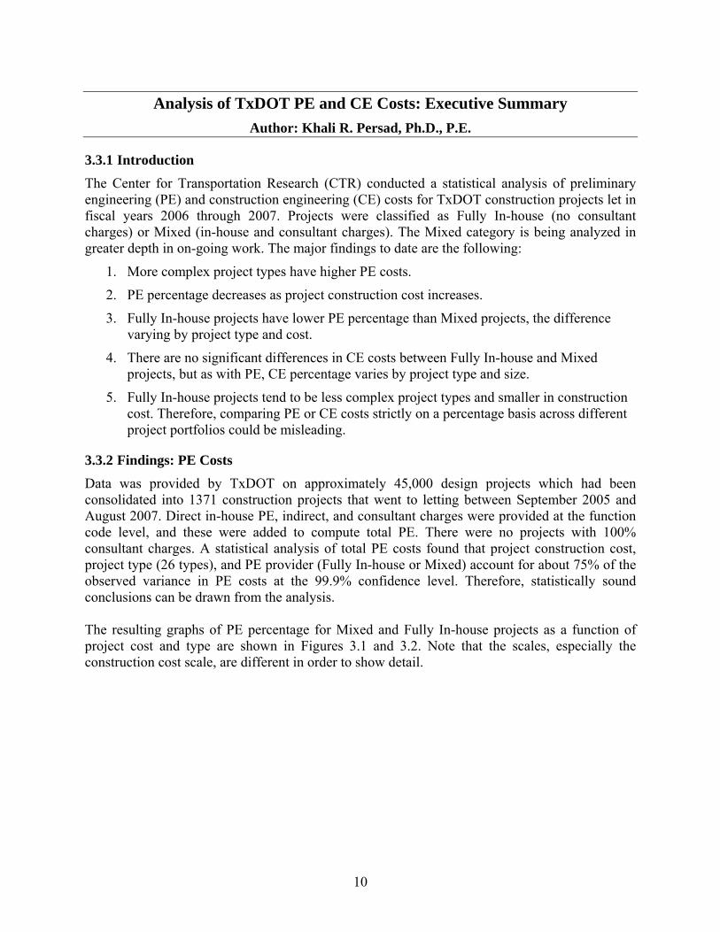
Analysis of TxDOT PE and CE Costs: Executive Summary Author: Khali R. Persad, Ph.D., P.E.

3.3.1 Introduction The Center for Transportation Research (CTR) conducted a statistical analysis of preliminary engineering (PE) and construction engineering (CE) costs for TxDOT construction projects let in fiscal years 2006 through 2007. Projects were classified as Fully In-house (no consultant charges) or Mixed (in-house and consultant charges). The Mixed category is being analyzed in greater depth in on-going work. The major findings to date are the following:

1. More complex project types have higher PE costs.

2. PE percentage decreases as project construction cost increases.

3. Fully In-house projects have lower PE percentage than Mixed projects, the difference varying by project type and cost.

4. There are no significant differences in CE costs between Fully In-house and Mixed projects, but as with PE, CE percentage varies by project type and size.

5. Fully In-house projects tend to be less complex project types and smaller in construction cost. Therefore, comparing PE or CE costs strictly on a percentage basis across different project portfolios could be misleading.

3.3.2 Findings: PE Costs Data was provided by TxDOT on approximately 45,000 design projects which had been consolidated into 1371 construction projects that went to letting between September 2005 and August 2007. Direct in-house PE, indirect, and consultant charges were provided at the function code level, and these were added to compute total PE. There were no projects with 100% consultant charges. A statistical analysis of total PE costs found that project construction cost, project type (26 types), and PE provider (Fully In-house or Mixed) account for about 75% of the observed variance in PE costs at the 99.9% confidence level. Therefore, statistically sound conclusions can be drawn from the analysis. The resulting graphs of PE percentage for Mixed and Fully In-house projects as a function of project cost and type are shown in Figures 3.1 and 3.2. Note that the scales, especially the construction cost scale, are different in order to show detail.

11

Figure 3.1: Estimated PE Percentage for Projects with Consultant Involvement

Figure 3.2: Estimated PE Percentage for Projects without Consultant Involvement

12

For both In-house and Mixed PE projects and for all project types, PE percentage decreases as project construction cost increases. For each project type of a given cost, the In-house PE percentage is estimated to be less than that of a Mixed project, but by a factor that varies. In gross terms, PE percentage for In-house and Mixed projects is 1.29% and 6.20% respectively for the full set of projects studied. Project types were found to rank from most to least costly as follows: 1. WF- Widen Freeway (including NLF-New Location Freeway and CNF Convert Non-Freeway to Freeway), 2. UPG- Upgrade Freeway to Standards, 3. INC- Interchange, 4. BR-Bridge Replacement, 5. BWR- Bridge Widen/Rehab, 6. WNF- Widen Non-Freeway, 7. MSC- Miscellaneous Construction, 8. Other, 9. Landscape, 10. Overlays, and 11. Sealcoats. The “Other” category includes those project types not named. This list can also be interpreted as a ranking of project complexity, and generally, Fully In-house projects are the less complex project types. In-house projects are also typically smaller in construction cost, which may be treated as a proxy for project size or scope. This analysis found that PE costs as recorded by TxDOT depend on project scope and complexity. TxDOT projects with consultant involvement are typically larger in scope and more complex, and are more costly. Therefore, computing a gross percentage PE without considering the scope and complexity of individual projects could give a false picture of relative costs of consultants versus in-house.

3.3.3 Findings: CE Costs In the CE cost analysis, it was found that project construction cost and project type account for about 72% of the variance in CE costs. No statistically significant difference in costs was found between Fully In-House and Mixed CE projects, perhaps because the number of Mixed CE projects is very small. Project types were found to rank as follows, from most to least costly: Traffic Signals, Bridge Replacement, Landscape, Other, Overlays, and Sealcoats. For all project types the percentage CE decreases as project cost increases. In gross terms, CE percentage is 4.03% for the full set of projects studied. As with PE costs, giving a gross percentage CE without considering the scope and complexity of individual projects could give a false picture of relative costs.

3.3.4 Comparison of Texas to Other States According to a 2006 U.S. General Accounting Office (GAO) survey, 15 state Departments of Transportation (DOTs) outsource more than 50% of their PE work. Of the larger DOTs, Florida is out front, planning to outsource 84% of its PE work in the period 2009-2013. In fact, Florida hires consultants to review other consultants’ work. On the projects analyzed for this report, TxDOT spent $471 million on PE, of which about 35% was in-house charges, 5% was indirect costs, and about 60% was consultant charges. However, these reported percentages are of dollars recorded by the DOTs as spent on PE. While DOTs have adequate systems for recording consultant costs, the GAO noted that most states do not have adequate accounting systems to record in-house charges at the project level or to track and allocate charges as projects move from conception to construction. As a result, DOTs may be underreporting in-house costs. Over the years there have been several surveys of DOT percentage PE and CE costs for in-house and consultant work. In the majority of these surveys, reported PE cost in-house is lower. For example, in late 2008, TxDOT conducted such a survey and found that the national in-house PE

13

percentage range is 3.18-10%, with Texas being the lowest. The range of consultant PE percentage is 6-16%, with Texas at 8.65%. However, as was seen in the statistical analysis above, these percentages can be misleading without knowing what size and type of projects are included in each. Another complication is the definition of a consultant project. Many analysts choose an arbitrary divider. For example, if more than 50% of the PE cost went to the consultant then it is a consultant project. Instead, it may be useful to consider the relative outputs and the premium paid. These issues are being explored in continuing work on this research. The 2008 TxDOT survey of CE costs found that the range for in-house work is 3.75-20%, with Texas at 4.5%. The range for consultant CE is 10-15%, with Texas at 10.7%. As with the PE percentages, these numbers can be misleading without knowing what size, type, and number of projects are included.

3.3.5 Outsourcing: Cost Versus Other Considerations Over the last 30 years, DOTs have seen an increasing trend of outsourcing PE and CE work. A number of forces are driving this trend, including these seven:

1. Loss of in-house staff: DOTs have experienced a shortage of skilled staff due to retirements, wage freezes, and attraction to the private sector.

2. Variations in workload: DOTs have seen rapid changes in workload due to fluctuations in state and federal funding. It is not possible to change in-house staff levels so quickly.

3. Specialized skills and equipment: In-house personnel are familiar with typical projects but may need expert help on specialized work. Limited frequency of these projects may not warrant keeping the relevant skills in-house.

4. Schedule constraints: Consultants may be able to “load up” a project and execute it very quickly, whereas in-house staff juggling a large number of projects on a “first-in, first-out” basis generally cannot. When speed is required, consultants are the preferred choice.

5. Legal and policy requirements. Some state legislatures limit the state work force, while some, such as Illinois and Texas, must outsource a certain fraction of their work.

6. Innovations: The private sector is better at innovating, partly because of less stringent rules than the public sector on equipment replacement and authority to use experimental techniques.

7. Cost savings: It is uneconomic for state DOTs to maintain a workforce large enough for peak workload conditions. Instead, work beyond some volume can be more cost-effectively done by consultants.

In 2006 the GAO asked state DOTs to rank the importance of these factors in the outsourcing decision. The rank order turned out to be as listed above, with cost savings being the least consideration. Only three DOTs considered cost savings to be an important factor in the outsourcing decision. In any case, state and federal laws prevent the consideration of cost as a factor in hiring professional services. This finding suggests that focusing on cost misses the

14

bigger picture. DOTs have no choice but to outsource because of workload variations, staff shortages, and schedule demands.

3.3.6 Conclusions Based on data provided by TxDOT, for each project type of a given cost, the In-house PE percentage is estimated to be less than that of a Mixed (in-house and consultant) project. The Mixed category is being analyzed in greater depth in on-going work. However, it appears that the need for specific skills and the ability to perform large projects on demand are important factors in PE costs. Therefore, estimating a percentage PE without considering the scope and complexity of individual projects could give a false picture of relative costs of consultants versus in-house. Instead of debating who is cheaper, DOTs need a rational approach to which projects and what portion of work should be done in-house and what and how much should be outsourced. Such an approach should consider several factors, including:

1. The minimum in-house staff and skills required to maintain competency in managing the construction program and monitoring consultants.

2. The types and sizes of projects that have to be done in-house to train and retain such a cadre of experts for management positions.

3. The premium paid for consultants for unique capabilities and for being “on-call,” and

4. The total cost of the “make or buy decision,” including the cost of delays.

CTR proposes to undertake the development of such an approach as a separate task in this research project, if TxDOT Administration approves. [Note: This recommendation was approved as a separate task to be completed in February 2010].

3.3.7 References Texas Department of Transportation (TxDOT). (Summer 2007). TxDOT: Open for Business. Retrieved

May 15, 2008, from: http://www.txdot.gov/publications/government_and_public_affairs/open_for_business.pdf

TxDOT, 2008: Texas Department of Transportation Website: http://www.dot.state.tx.us/projectselection. Accessed February 2008

TxDOT, Keep Texas Moving: Why We are Doing It. Website: http://www.keeptexasmoving.com/index.php/why_are_we_doing_it

3.4 In-Depth Report Following is the in-depth report that was submitted by CTR for this task in September 2009.

15

An Analysis of TxDOT's In-house and Consultant Preliminary Engineering (PE) and Construction Engineering (CE) Costs

Authors: Khali R. Persad & Prakash Singh

3.5 Introduction This report examines available TxDOT data on in-house preliminary engineering (PE) and consultant PE costs as well as construction engineering (CE) costs, and provides comparisons and findings. This research was conducted between December 2008 and August 2009.

3.5.1 Background There has been a perennial debate over the efficiency of state departments of transportation (DOTs) in performing PE in-house compared to outsourcing the work to consultants. In recent years, that debate has extended to construction management work, as legislators have encouraged DOTs to privatize some of their construction inspection and management operations. The 2008 Sunset Review of the Texas DOT (TxDOT) brought renewed calls for “improvements in efficiency” and simultaneously queried TxDOT’s expenditures for consultants. Complicating the issue further are the facts that, by law TxDOT is required to hire engineering consultants for a certain amount of work, and selection must be based on qualifications and not on cost. In this context, TxDOT’s primary need was an assessment of its costs for delivering projects, both in-house and through consultants. To address this need, TxDOT assembled a group of experienced resource persons, who established contacts with several other state DOTs, collected a significant amount of data, and conducted some analyses of costs. TxDOT then enlisted researchers at the Center for Transportation Research (CTR) to complement the work of the TxDOT resource team in analyzing TxDOT PE and CE costs. Staff at CTR has been researching similar questions for many years. In 1989, Dr. Khali Persad analyzed TxDOT PE costs for projects in the period from 1986-1988 and developed curves of PE as a percentage of construction cost by project type. In 1995-1996, as part of a TxDOT task force headed by former Deputy Executive Director Robert Cuellar, he compared in-house PE costs to consultant costs using FIMS data.

3.5.2 Research Approach

The primary aim of the work documented here was to conduct statistical analyses of TxDOT data. This research was conducted in two phases: a fast turnaround with preliminary results (submitted in February 2009), and a medium-term effort as documented in this report.

1. Fast turnaround analysis: Analyze data that can be collected or accessed quickly, to provide a comparison of TxDOT’s PE and CE costs for in-house and consultant projects.

2. Medium term study: Analyze TxDOT data in-depth and create PE and CE performance measures that would allow intra-agency diagnostics as well as extra-agency comparisons.

Four issues are addressed in this analysis:

16

1. The cost of engineering for projects done with in-house staff compared to using consultant forces.

2. The differences in engineering costs for different project types and across a range of work scopes.

3. The quality of engineering for projects done with in-house staff compared to using consultant forces.

4. The differences in engineering costs across TxDOT districts.

3.5.3 Organization of Report This report is organized in eight sections. This section provided the research background and scope. Section 3.6 describes the data analyzed and the statistical methodology used. Section 3.7 provides a comparison of in-house PE costs to projects with consultant involvement. Section 3.8 goes in-depth into costs at the design function level. Section 3.10 gives an analysis of the costs of change orders for in-house and consultant projects. Section 3.11 contains the results of cross-district comparisons of PE costs. Section 3.12 provides a comparison of in-house CE costs to projects with consultant involvement. Section 3.13 provides conclusions and recommendations.

3.6 Data Description and Analysis Methodology This section provides a description of the data obtained from TxDOT and the methodology used for data analysis. Actual charges for PE and CE for projects let in fiscal years 2006 and 2007 (FY 06-07: September 2005–August 2007) were obtained from TxDOT’s Construction Division and Finance Division.

3.6.1 Data Summary Table 3.1 is a summary of the projects by project type. Construction cost was computed as the sum of contract letting amount plus net change orders.

17

Table 3.1: Summary of TxDOT contracts let in FY 06-07

Project Type Code Project Type Description No of

Projects (Contract Amount + Change Orders)

BCF Border Crossing Facility 1 $4,345,638.04BR Bridge Replacement 236 $608,983,868.40BWR Bridge Widening Or 55 $222,272,397.38CNF Convert Non-Freeway To Freeway 7 $301,692,143.84CTM Corridor Traffic Management 14 $62,471,234.99FBO Ferry Boat 1 $22,512,000.00HES Hazard Elimination & Safety 4 $5,240,528.55INC Interchange (New or 28 $787,298,018.28LSE Landscape and Scenic 83 $41,463,949.04MSC Miscellaneous Construction 349 $818,837,999.76NLF New Location Freeway 1 $67,466,929.41NNF New Location Non-Freeway 12 $193,373,350.63OV Overlay 184 $611,568,634.47RER Rehabilitation of Existing Road 192 $1,013,188,529.29RES Restoration 50 $167,257,222.79ROW Right of Way 2 $146,173,826.42SC Seal Coat 85 $460,855,529.66SFT Safety Project 311 $1,064,450,294.13

SKP SKIP (Exempt from sealing – Transportation Enhancement

6 $8,488,995.93

SRA Safety Rest Area 3 $42,035,563.16TC Tunnel Construction 1 $165,509.87TDP Traffic Protection Devices 4 $8,214,080.41TS Traffic Signal 57 $31,839,098.29UGN Upgrade to Standards Non- 13 $68,956,309.65UPG Upgrade to Standards Freeway 12 $186,878,396.43WF Widen Freeway 14 $825,697,696.07WNF Widen Non-Freeway 70 $1,049,760,200.79Total 1795 $8,821,487,945.68

In terms of frequency of project types, the top ten in order are MSC, SFT, BR, RER, OV, SC, LSE, WNF, TS, and BWR. In terms of dollar volume, the top ten in order are SFT, WNF, RER, WF, MSC, INC, OV, BR, SC, and CNF. The analysis will pay particular attention to these project types. Apart from the above set of 1,795 projects, TxDOT provided another list of 65 contracts that were tagged as Exceptions. Upon review, it was found that 28 of the Exceptions were also included in the first list. After removing the repeats, there was data on 1,832 (1795+65-28=1832) projects.

18

3.6.2 Function Codes TxDOT PE charges are collected at the function code level for each design job (Control Section Job (CSJ)). Table 3.2 lists the function codes used by TxDOT for PE accounting.

Table 3.2: TxDOT Function Codes for PE Charges Function Code Function Description

102 Feasibility Studies 110 Route and Design Studies 120 Social, Economic and Environmental Studies and Public Involvement 126 Donated Items or Services 130 Right -of-Way Data (State or Contract Provided)

145

Managing Contracted or Donated Advance PE Services. Also includes all costs to acquire the consultant contract(s) and services Applicable to advance PE, Function Codes 102 -150. Advance PE are activities in Function Codes 102 through 150.

146 Rework by TxDOT of complete consultant plans on advance PE projects. Advance PE are activities in function codes 102 through 150.

150 Field Surveying and Photogrammetry 160 Roadway Design Controls (Computations and Drafting) 161 Drainage 162 Signing, Pavement Markings, Signalization (Permanent) 163 Miscellaneous (Roadway)

164

Managing Contracted or donated PS & E PE Services. Also includes all costs to acquire the Consultants Contract(s) and Services applicable to PS & E, Function Codes 160 - 190. PS & E PE are activities in function code 160 through 190.

165 Traffic Management Systems (Permanent)

166

Rework By TxDOT Of Completed Consultant Plans on PE & E projects. PS & E PE are activities in function codes 160 through 190. Rework Segment 76 FCs 160-190 for metric conversion. For reworking existing PS&E to metric units on projects already into plan preparation.

169 Donated Items or Services 170 Bridge Design 180 District Design Review and Processing 181 Austin Office Processing (State Prepared P.S. & E.) 182 Austin Office Processing (Consultant Prepared P.S. & E.) 190 Other Pre-letting date Charges, Not Otherwise Classified. 191 Toll Feasibility Studies 192 Comprehensive Development Agreement Procurement 193 Toll Collection Planning

19

3.6.3 PE Charges A TxDOT construction contract (Contract Control Section Job (CCSJ)) includes one or more design jobs (CSJ). TxDOT categorizes PE charges as Consultant PE, Indirect PE, or In-house PE costs. The total PE cost for a construction contract was computed as the sum of all PE charges (functions codes 100-199) in all design CSJs that had been combined into the CCSJ for letting. TxDOT provided a status for each contract, namely, Closed (account finalized), Closing (account not finalized), Inactive (pending resolution), and Open (accounts still being charged). Table 3.3 is a summary of the PE totals for all 1,832 projects.

Table 3.3: PE totals for TxDOT construction contracts let in FY 06-07

Project Type Status Total PE Life-to-Date

Consultant PE Costs

Indirect PE Costs

In-house PE Costs

Bridge Replacement

Closed $10,322,188.38 $6,250,806.64 $598,306.81 $3,473,074.93 Closing $12,759.18 $455.53 $589.94 $11,713.71 Inactive $18,821,527.61 $12,410,483.36 $979,069.73 $5,431,974.52

Open $24,800,985.62 $16,460,358.73 $1,314,432.88 $7,026,194.01 Total $53,957,460.79 $35,122,104.26 $2,892,399.36 $15,942,957.17

Ferry Open $1,708,164.41 $1,649,330.17 $56,294.91 $2,539.33 Total $1,708,164.41 $1,649,330.17 $56,294.91 $2,539.33

Landscape/ Scenic

Enhancement

Closed $554,047.46 $69,779.42 $26,463.52 $457,804.52 Inactive $131,870.80 $0.00 $8,346.06 $123,524.74

Open $554,111.28 $0.00 $23,825.99 $530,285.29 Total $1,240,029.54 $69,779.42 $58,635.57 $1,111,614.55

Border Crossing

Facility

Open $173,263.78 $149,377.13 $10,123.55 $13,763.10

Total $173,263.78 $149,377.13 $10,123.55 $13,763.10

ROW Total 0 0 0 0

Seal Coat

Closed $1,550,173.83 $30,897.64 $76,515.79 $1,442,760.40 Inactive $90,239.55 $51,891.68 $3,521.63 $34,826.24

Open $357,106.90 $7,109.50 $17,089.29 $332,908.11 Total $1,997,520.28 $89,898.82 $97,126.71 $1,810,494.75

Tunnel Construction

Closed $117,895.41 $107,494.68 $3,824.87 $6,575.86 Total $117,895.41 $107,494.68 $3,824.87 $6,575.86

Traffic Protection

Devices

Inactive $302,362.60 $258,756.60 $10,238.99 $33,367.01 Open $124,283.94 $46,281.62 $5,863.08 $72,139.24 Total $426,646.54 $305,038.22 $16,102.07 $105,506.25

Upgrade to Standards

Freeway

Closed $1,941,866.88 $248,420.64 $91,545.40 $1,601,900.84 Inactive $462,046.45 $97,572.41 $25,364.97 $339,109.07

Open $2,327,521.29 $540,632.87 $94,157.29 $1,692,731.13 Total $4,731,434.62 $886,625.92 $211,067.66 $3,633,741.04

Bridge Widening or Rehabilitate

Closed $1,168,951.09 $499,892.61 $64,010.83 $605,047.65 Inactive $4,479,512.77 $2,943,916.78 $230,447.65 $1,305,148.34

Open $8,460,435.81 $5,602,488.28 $411,675.12 $2,446,272.41

20


Consultant PE Costs

Indirect PE Costs

In-house PE Costs

Total $14,108,899.67 $9,046,297.67 $706,133.60 $4,356,468.40

Convert Non-Freeway to

Freeway

Inactive $2,720,716.36 $1,110,662.82 $135,646.52 $1,474,407.02

Open $16,616,384.64 $12,632,079.53 $1,058,817.58 $2,925,487.53 Total $19,337,101.00 $13,742,742.35 $1,194,464.10 $4,399,894.55

Hazard Elimination &

Safety

Inactive $72,864.49 $0.00 $3,153.92 $69,710.57 Open $476,817.92 $359,389.82 $21,420.59 $96,007.51 Total $549,682.41 $359,389.82 $24,574.51 $165,718.08

Interchange (New or

Reconstruct)

Closed $44,215.77 $2,050.00 $1,635.66 $40,530.11 Inactive $372,351.44 $313,569.03 $17,890.23 $40,892.18

Open $40,631,770.11 $24,824,184.80 $2,183,660.95 $13,623,924.36 Total $41,048,337.32 $25,139,803.83 $2,203,186.84 $13,705,346.65

New Location Freeway

Open $13,849,319.31 $11,473,259.35 $678,202.81 $1,697,857.15 Total $13,849,319.31 $11,473,259.35 $678,202.81 $1,697,857.15

New Location Non-Freeway

Inactive $247,336.48 $68,231.45 $11,270.25 $167,834.78 Open $7,498,294.75 $4,309,574.10 $435,445.36 $2,753,275.29 Total $7,745,631.23 $4,377,805.55 $446,715.61 $2,921,110.07

Overlay

Closed $4,195,393.95 $1,156,833.65 $238,627.62 $2,799,932.68 Inactive $2,230,735.86 $259,666.03 $104,886.17 $1,866,183.66

Open $4,478,210.37 $1,026,054.55 $199,302.38 $3,252,853.44 Total $10,904,340.18 $2,442,554.23 $542,816.17 $7,918,969.78

Rehabilitate Existing Roads

Closed $6,824,111.73 $3,588,677.13 $367,113.04 $2,868,321.56 Inactive $14,933,771.11 $7,583,143.32 $864,915.64 $6,485,712.15

Open $33,772,199.74 $23,096,092.75 $1,793,997.20 $8,882,109.79 Total $55,530,082.58 $34,267,913.20 $3,026,025.88 $18,236,143.50

All Safety Bond Program

Closed $16,792,631.71 $9,228,494.07 $832,079.22 $6,732,058.42 Inactive $5,626,212.63 $2,948,471.92 $281,299.91 $2,396,440.80

Open $28,195,286.22 $18,519,345.25 $1,362,250.32 $8,313,690.65 Total $50,614,130.56 $30,696,311.24 $2,475,629.45 $17,442,189.87

Safety Rest Area

Open $3,485,582.31 $1,202,273.24 $204,650.45 $2,078,658.62 Total $3,485,582.31 $1,202,273.24 $204,650.45 $2,078,658.62

Traffic Signal

Closed $863,419.79 $409,229.38 $44,193.11 $409,997.30 Inactive $693,931.12 $300,885.33 $33,819.10 $359,226.69

Open $1,762,387.86 $1,098,558.48 $84,993.49 $578,835.89 Total $3,319,738.77 $1,808,673.19 $163,005.70 $1,348,059.88

Upgrade to Standards Non-

Freeway

Closed $89,962.15 $0.00 $7,327.66 $82,634.49 Inactive $1,436,926.85 $824,652.06 $102,369.70 $509,905.09

Open $5,953,036.71 $2,482,276.20 $379,764.13 $3,090,996.38 Total $7,479,925.71 $3,306,928.26 $489,461.49 $3,683,535.96

Widening Freeway

Closed $26,805.55 $0.00 $1,100.39 $25,705.16 Inactive $47,958.75 $0.00 $2,222.35 $45,736.40

21


Consultant PE Costs

Indirect PE Costs

In-house PE Costs

Open $38,005,017.58 $21,187,580.12 $1,913,864.64 $14,903,572.82 Total $38,079,781.88 $21,187,580.12 $1,917,187.38 $14,975,014.38

Widening Non-Freeway

Closed $1,502,658.65 $739,441.74 $80,767.36 $682,449.55 Inactive $1,670,287.15 $1,159,906.59 $98,296.56 $412,084.00

Open $72,062,639.22 $46,628,380.54 $4,028,239.57 $21,406,019.11 Total $75,235,585.02 $48,527,728.87 $4,207,303.49 $22,500,552.66

Corridor Traffic

Management

Closed $151,455.26 $102,701.80 $7,012.55 $41,740.91 Inactive $74,702.16 $0.00 $2,586.66 $72,115.50

Open $2,043,176.27 $609,676.76 $92,227.01 $1,341,272.50 Total $2,269,333.69 $712,378.56 $101,826.22 $1,455,128.91

Utility Adjustments Total 0 0 0 0

SKIP (Transp. Enh. Program)

Inactive $129,369.22 $91,339.10 $5,546.28 $32,483.84 Total $129,369.22 $91,339.10 $5,546.28 $32,483.84

Restoration

Closed $2,664,983.40 $1,140,746.49 $140,681.42 $1,383,555.49 Closing $108,203.59 $49,839.65 $5,695.74 $52,668.20 Inactive $1,955,687.73 $873,914.30 $96,297.37 $985,476.06

Open $3,012,753.23 $1,514,975.48 $149,452.18 $1,348,325.57 Total $7,741,627.95 $3,579,475.92 $392,126.71 $3,770,025.32

Bridge Preventive Mnt Total 0 0 0 0

Bridge Preventive Mnt

- Sealed

Open $523.49 $0.00 $33.18 $490.31

Total $523.49 $0.00 $33.18 $490.31

Misc Construction

Closed $8,893,208.92 $3,669,638.51 $443,042.28 $4,780,528.13 Closing $127,122.82 $0.00 $5,257.56 $121,865.26 Inactive $5,623,854.53 $2,089,295.54 $263,298.34 $3,271,260.65

Open $40,176,737.92 $23,144,170.17 $1,973,505.99 $15,059,061.76 Total $54,820,924.19 $28,903,104.22 $2,685,104.17 $23,232,715.80

Grand Total $470,602,331.86 $279,245,207.34 $24,809,568.74 $166,547,555.78 Total Closed $57,703,969.93 $27,245,104.40 $3,024,247.53 $27,434,618.00

Total Closing $248,085.59 $50,295.18 $11,543.24 $186,247.17Total Inactive $62,124,265.66 $33,386,358.32 $3,280,488.03 $25,457,419.31

Total Open $350,526,010.68 $218,563,449.44 $18,493,289.94 $113,469,271.30 Out of a total of about $471 million spent on PE for these 1,832 projects, about 60% was consultant charges, 35% was in-house charges, and 5% was indirect costs.

3.6.4 CE Charges

The total CE cost for a project was computed as the sum of consultant, in-house, and indirect charges for that CCSJ. Table 3.4 is a summary of the CE charges for 1,832 projects.

22

Table 3.4: CE totals for TxDOT construction contracts let in FY 06-07

Project Type Status Total CE Life-to-Date

Consultant CE Costs

Indirect CE Costs

In-house CE Costs

Bridge Replacement

Closed $4,745,065.46 $275,317.28 $226,995.46 $4,242,752.72 Closing $36,323.33 $1,685.22 $1,747.96 $32,890.15 Inactive $8,888,027.21 $244,742.38 $440,348.75 $8,202,936.08 Open $12,765,883.37 $395,417.76 $594,139.99 $11,776,325.62 Total $26,435,299.37 $917,162.64 $1,263,232.16 $24,254,904.57

Ferry Open $57,244.41 $0.00 $1,567.87 $55,676.54 Total $57,244.41 $0.00 $1,567.87 $55,676.54

Landscape/Scenic Enhancement

Closed $1,131,479.29 $6,063.25 $56,423.47 $1,068,992.57 Inactive $348,315.33 $1,162.03 $25,113.09 $322,040.21 Open $1,515,993.20 $736.52 $56,727.41 $1,458,529.27 Total $2,995,787.82 $7,961.80 $138,263.97 $2,849,562.05

Border Crossing Fac

Open $37,743.17 $0.00 $1,141.97 $36,601.20 Total $37,743.17 $0.00 $1,141.97 $36,601.20

ROW Open $468,612.53 $75,564.41 $18,197.85 $374,850.27 Total $468,612.53 $75,564.41 $18,197.85 $374,850.27

Seal Coat

Closed $8,037,501.96 $117,968.69 $409,581.38 $7,509,951.89 Inactive $151,034.61 $229.41 $7,302.15 $143,503.05 Open $2,778,337.45 $343,305.81 $142,473.11 $2,292,558.53 Total $10,966,874.02 $461,503.91 $559,356.64 $9,946,013.47

Tunnel Construction

Closed $8,741.45 $0.00 $308.57 $8,432.88 Total $8,741.45 $0.00 $308.57 $8,432.88

Traffic Protection Devices

Inactive $120,394.11 $0.00 $4,561.19 $115,832.92 Open $261,585.20 $0.00 $9,806.03 $251,779.17 Total $381,979.31 $0.00 $14,367.22 $367,612.09

Upgrade to Standards Freeway

Closed $1,010,162.66 $5,318.50 $54,493.10 $950,351.06 Inactive $1,268,516.15 $1,035.00 $70,236.57 $1,197,244.58 Open $2,241,948.53 $40,137.06 $97,857.97 $2,103,953.50 Total $4,520,627.34 $46,490.56 $222,587.64 $4,251,549.14

Bridge Widening or Rehabilitate

Closed $1,169,123.74 $44,854.99 $56,672.65 $1,067,596.10 Inactive $2,712,701.90 $105,924.62 $127,250.00 $2,479,527.28 Open $4,613,620.55 $223,149.71 $209,413.17 $4,181,057.67 Total $8,495,446.19 $373,929.32 $393,335.82 $7,728,181.05

Convert Non-Freeway to Freeway

Inactive $180,796.43 $20,895.95 $6,809.86 $153,090.62 Open $7,174,798.01 $386,528.50 $342,963.47 $6,445,306.04 Total $7,355,594.44 $407,424.45 $349,773.33 $6,598,396.66

Hazard Elimination & Safety

Inactive $80,760.59 $0.00 $3,617.90 $77,142.69 Open $268,088.17 $0.00 $11,371.85 $256,716.32 Total $348,848.76 $0.00 $14,989.75 $333,859.01

Interchange (New or Reconstruct)

Closed $194,476.66 $1,586.00 $9,502.00 $183,388.66 Inactive $255,978.02 $39,439.28 $13,361.01 $203,177.73 Open $20,560,535.20 $2,074,298.14 $842,496.20 $17,643,740.86 Total $21,010,989.88 $2,115,323.42 $865,359.21 $18,030,307.25

New Location Freeway

Open $5,623,182.01 $414,829.32 $262,318.60 $4,946,034.09 Total $5,623,182.01 $414,829.32 $262,318.60 $4,946,034.09

23


Consultant CE Costs

Indirect CE Costs

In-house CE Costs

New Location Non-Freeway

Inactive $203,890.20 $347.00 $8,233.85 $195,309.35 Open $3,807,571.02 $361,501.85 $174,348.53 $3,271,720.64 Total $4,011,461.22 $361,848.85 $182,582.38 $3,467,029.99

Overlay

Closed $9,879,016.40 $931,126.77 $486,782.27 $8,461,107.36 Inactive $6,698,447.10 $251,202.52 $332,630.43 $6,114,614.15 Open $5,472,153.29 $497,338.00 $240,682.83 $4,734,132.46 Total $22,049,616.79 $1,679,667.29 $1,060,095.53 $19,309,853.97

Rehabilitate Existing Roads

Closed $7,600,429.12 $216,679.37 $393,435.93 $6,990,313.82 Inactive $13,084,555.98 $765,758.07 $689,500.38 $11,629,297.53 Open $23,452,632.16 $1,473,596.06 $1,162,767.16 $20,816,268.94 Total $44,137,617.26 $2,456,033.50 $2,245,703.47 $39,435,880.29

All Safety Bond Program

Closed $12,445,244.99 $333,281.41 $597,429.28 $11,514,534.30 Inactive $5,653,161.47 $97,372.32 $267,891.19 $5,287,897.96 Open $17,969,331.52 $608,947.89 $827,432.69 $16,532,950.94 Total $36,067,737.98 $1,039,601.62 $1,692,753.16 $33,335,383.20

Safety Rest Area

Open $1,241,866.30 $15,567.60 $57,997.78 $1,168,300.92 Total $1,241,866.30 $15,567.60 $57,997.78 $1,168,300.92

Traffic Signal

Closed $1,150,624.74 $12,684.16 $55,557.54 $1,082,383.04 Inactive $712,329.22 $1,944.72 $33,255.13 $677,129.37 Open $2,232,291.21 $2,120.32 $96,066.58 $2,134,104.31 Total $4,095,245.17 $16,749.20 $184,879.25 $3,893,616.72

Upgrade to Standards Non-Freeway

Closed $97,497.67 $0.00 $7,287.62 $90,210.05 Inactive $642,475.84 $5,017.00 $42,084.61 $595,374.23 Open $2,752,876.41 $104,734.26 $142,682.12 $2,505,460.03 Total $3,492,849.92 $109,751.26 $192,054.35 $3,191,044.31

Widening Freeway

Closed $312,976.53 $775.54 $10,737.66 $301,463.33 Inactive $509,504.92 $24,373.04 $26,335.23 $458,796.65 Open $15,732,895.63 $1,422,233.59 $613,150.75 $13,697,511.29 Total $16,555,377.08 $1,447,382.17 $650,223.64 $14,457,771.27

Widening Non-Freeway

Closed $933,913.07 $65,762.26 $40,109.57 $828,041.24 Inactive $1,296,815.71 $65,381.63 $57,926.03 $1,173,508.05 Open $31,153,631.20 $2,642,633.10 $1,361,795.73 $27,149,202.37 Total $33,384,359.98 $2,773,776.99 $1,459,831.33 $29,150,751.66

Corridor Traffic Management

Closed $102,023.43 $0.00 $5,198.88 $96,824.55 Inactive $20,153.40 $5,848.23 $663.96 $13,641.21 Open $1,725,314.80 $33,496.69 $61,602.52 $1,630,215.59 Total $1,847,491.63 $39,344.92 $67,465.36 $1,740,681.35

Utility Adjustments

Inactive $26,856.84 $2,995.15 $1,013.82 $22,847.87 Open $534,715.83 $115,077.45 $19,437.30 $400,201.08 Total $561,572.67 $118,072.60 $20,451.12 $423,048.95

SKIP (Exempt from sealing – Transp. Enh. Program

Inactive $416,920.51 $133,631.57 $23,475.08 $259,813.86

Total $416,920.51 $133,631.57 $23,475.08 $259,813.86

Restoration Closed $2,785,642.61 $38,127.25 $127,337.56 $2,620,177.80 Closing $202,937.49 $0.00 $8,850.85 $194,086.64 Inactive $1,935,977.43 $97,077.78 $87,046.35 $1,751,853.30

24


Consultant CE Costs

Indirect CE Costs

In-house CE Costs

Open $3,831,781.81 $134,155.04 $193,736.05 $3,503,890.72 Total $8,756,339.34 $269,360.07 $416,970.81 $8,070,008.46

Bridge Preventive Mnt - Not Sealed

Open $547.24 $0.00 $24.61 $522.63

Total $547.24 $0.00 $24.61 $522.63 Bridge Preventive Mnt - Sealed

Open $127,468.34 $0.00 $6,754.77 $120,713.57

Total $127,468.34 $0.00 $6,754.77 $120,713.57

Misc Construction

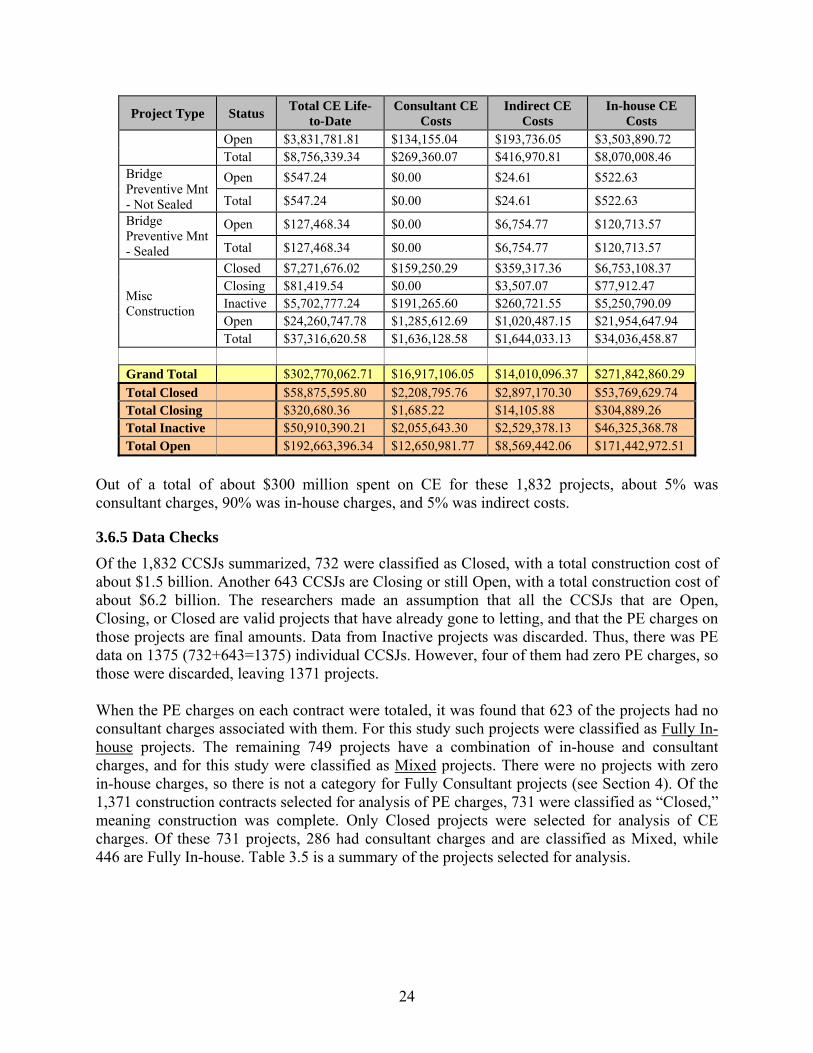
Closed $7,271,676.02 $159,250.29 $359,317.36 $6,753,108.37 Closing $81,419.54 $0.00 $3,507.07 $77,912.47 Inactive $5,702,777.24 $191,265.60 $260,721.55 $5,250,790.09 Open $24,260,747.78 $1,285,612.69 $1,020,487.15 $21,954,647.94 Total $37,316,620.58 $1,636,128.58 $1,644,033.13 $34,036,458.87

Grand Total $302,770,062.71 $16,917,106.05 $14,010,096.37 $271,842,860.29 Total Closed $58,875,595.80 $2,208,795.76 $2,897,170.30 $53,769,629.74 Total Closing $320,680.36 $1,685.22 $14,105.88 $304,889.26 Total Inactive $50,910,390.21 $2,055,643.30 $2,529,378.13 $46,325,368.78 Total Open $192,663,396.34 $12,650,981.77 $8,569,442.06 $171,442,972.51

Out of a total of about $300 million spent on CE for these 1,832 projects, about 5% was consultant charges, 90% was in-house charges, and 5% was indirect costs.

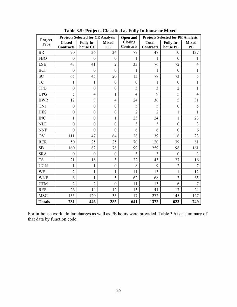
3.6.5 Data Checks Of the 1,832 CCSJs summarized, 732 were classified as Closed, with a total construction cost of about $1.5 billion. Another 643 CCSJs are Closing or still Open, with a total construction cost of about $6.2 billion. The researchers made an assumption that all the CCSJs that are Open, Closing, or Closed are valid projects that have already gone to letting, and that the PE charges on those projects are final amounts. Data from Inactive projects was discarded. Thus, there was PE data on 1375 (732+643=1375) individual CCSJs. However, four of them had zero PE charges, so those were discarded, leaving 1371 projects. When the PE charges on each contract were totaled, it was found that 623 of the projects had no consultant charges associated with them. For this study such projects were classified as Fully In-house projects. The remaining 749 projects have a combination of in-house and consultant charges, and for this study were classified as Mixed projects. There were no projects with zero in-house charges, so there is not a category for Fully Consultant projects (see Section 4). Of the 1,371 construction contracts selected for analysis of PE charges, 731 were classified as “Closed,” meaning construction was complete. Only Closed projects were selected for analysis of CE charges. Of these 731 projects, 286 had consultant charges and are classified as Mixed, while 446 are Fully In-house. Table 3.5 is a summary of the projects selected for analysis.

25

Table 3.5: Projects Classified as Fully In-house or Mixed

Project Type

Projects Selected for CE Analysis Open and Closing

Contracts

Projects Selected for PE Analysis Closed

Contracts Fully In-house CE

Mixed CE

Total Contracts

Fully In-house PE

Mixed PE

BR 70 36 34 77 147 10 137FBO 0 0 0 1 1 0 1LSE 43 41 2 33 76 72 4BCF 0 0 0 1 1 0 1SC 65 45 20 13 78 73 5TC 1 1 0 0 1 0 1TPD 0 0 0 3 3 2 1UPG 5 4 1 4 9 5 4BWR 12 8 4 24 36 5 31CNF 0 0 0 5 5 0 5HES 0 0 0 2 2 1 1INC 1 0 1 23 24 1 23NLF 0 0 0 3 3 0 3NNF 0 0 0 6 6 0 6OV 111 47 64 28 139 116 23RER 50 25 25 70 120 39 81SB 160 82 78 99 259 98 161SRA 0 0 0 3 3 0 3TS 21 18 3 22 43 27 16UGN 1 1 0 8 9 2 7WF 2 1 1 11 13 1 12WNF 6 1 5 62 68 3 65CTM 2 2 0 11 13 6 7RES 26 14 12 15 41 17 24MSC 155 120 35 117 272 145 127Totals 731 446 285 641 1372 623 749

For in-house work, dollar charges as well as PE hours were provided. Table 3.6 is a summary of that data by function code.

26

Table 3.6: Summary of PE Charges by Function Code Func-tion

Total PE Life-to-Date

Indirect PE Charges

Consultant PE Charges

In-house PE Charges

In-house PE Hours

102 $1,056,099.07 $72,325.32 $582,595.14 $401,178.61 8637110 $32,268,964.61 $1,888,478.07 $19,682,670.97 $10,697,815.57 227699111 $0.00 $0.00 $0.00 $0.00 261117 $14,424.66 $1,115.59 $4,036.39 $9,272.68 288119 $0.00 $0.00 $0.00 $0.00 25120 $21,668,916.60 $1,172,520.06 $11,960,191.20 $8,536,205.34 143570130 $34,220,439.19 $1,939,444.44 $27,517,521.39 $4,763,473.36 105526140 $0.00 $0.00 $0.00 $0.00 66145 $4,446,376.34 $255,667.65 $638,710.56 $3,551,998.13 64678146 $128,382.32 $8,478.05 $0.00 $119,904.27 2857150 $53,751,613.18 $2,983,834.16 $42,923,276.59 $7,844,502.43 161520160 $54,414,967.90 $2,887,533.37 $31,425,140.65 $20,102,293.88 447008161 $32,873,018.57 $1,679,967.52 $24,274,696.84 $6,918,354.21 163878162 $19,369,025.86 $935,767.85 $11,884,560.74 $6,548,697.27 130515163 $75,122,028.10 $3,775,165.35 $37,923,406.48 $33,423,456.27 763170164 $23,511,987.55 $1,179,784.53 $11,124,012.04 $11,208,190.98 182446165 $4,762,558.08 $224,561.48 $1,579,193.53 $2,958,803.07 50106166 $204,722.40 $10,167.43 $0.00 $194,554.97 3649167 $2,179.72 $137.07 $0.00 $2,042.65 70170 $32,796,772.08 $1,663,301.81 $21,097,046.14 $10,036,424.13 207807180 $6,501,889.83 $301,190.45 $0.00 $6,200,699.38 118183181 $2,084,362.49 $97,201.98 $0.00 $1,987,160.51 50409182 $983,200.64 $43,323.12 $0.00 $939,877.52 23122183 $1,168.01 $84.17 $0.00 $1,083.84 20190 $6,293,481.45 $313,383.60 $2,029,565.06 $3,950,532.79 40567191 $559,474.26 $21,089.70 $538,384.56 $0.00 0192 $3,537.79 $200.25 $3,337.54 $0.00 0193 $129,840.07 $6,980.42 $122,859.65 $0.00 0195 $0.00 $0.00 $0.00 $0.00 2

3.6.6 Data Transforms During analysis, it was noted that the data exhibits log-normal distributions, i.e., a large number of projects have low values of PE and construction costs, and few projects have high values. To reduce modeling error, log transforms were used, i.e., the continuous variables were converted to their base 10 logarithm values. Where a value (e.g., PE cost) was found to be less than 1, it was changed to 1 to get a logarithm value of 0. This technique is commonly used to transform continuous variables. At worst, if the transform is not valid, the statistical relationship would return a coefficient close to 1, indicating there is no log-normal behavior. PE and CE costs were converted to LogPECost and LogCECost. Project construction cost was converted to LogConstructionCost. Project types were designated as binary or switch variables, i.e., a project type is present (value = 1) or absent (value = 0). Districts were similarly designated

27

as binary variables. Multiplicative interaction terms were also introduced to find model relationships that have different slopes for specific binary variables.

3.6.7 Data Analysis Methodology The objective of the analyses was to determine if there are differences in PE and CE costs for different groups, namely, between in-house and consultant, across project types, according to project cost, or across districts. The statistical technique chosen was stepwise regression. Stepwise regression is a particular type of regression analysis that also yields analysis of variance (ANOVA). After formulation of a general relationship between the dependent variable (PE or CE costs) and a provided set of independent variables, the independent variables are tested iteratively and automatically added to or removed from the model. Variables can be categorical (giving ANOVA), continuous (giving a regression equation), or interaction terms (which are products of other variables). Criteria for adding or removing variables are defined by the F-test. For this analysis, Fin was set at 3.84 and Fout at 2.71, equivalent to a statistical significance above 95% for entry and below 90% for removal. Variables are added iteratively and the partial F values are re-computed. If the significance of an ‘in’ variable falls below Fout it is removed. The process continues until there is no provided variable that can be added or removed. The analysis starts by identifying the provided independent variable with the highest F-value. If none are found, the analysis ends, giving the population mean of the dependent variable as the model estimate. A statistically significant categorical variable indicates that the presence of that variable divides the population, giving the same result as ANOVA. A statistically significant continuous variable indicates a linear relationship, and the intercept and slope of the relationship are calculated. The final model may contain categorical and continuous variables, as well as any of the interaction variables postulated. The coefficients of the variables in the model indicate their relative effect on the dependent variable. This method is able to find the best combination of provided independent variables to estimate the dependent variable, and was used in all the analyses presented later in this report. The SPSS statistical analysis program was used for the computations.

3.7 Comparison of Costs for In-house and Mixed Projects This section describes the results of a comparison of the cost of PE for projects done entirely in-house by TxDOT to the cost for projects done with consultant involvement. As discussed in the data description earlier, it was found that 623 PE projects had no consultant charges associated with them. For this study such projects were classified as Fully In-house projects. The remaining 749 projects have a combination of in-house and consultant charges, and for this study were classified as Mixed projects. There were no projects with zero in-house charges, so there is not a category for Fully Consultant projects (see Section 4). Therefore, this

28

analysis compares 749 Mixed projects to 623 Fully In-house projects, a sufficient sample to determine if there are statistical differences between the groups.

3.7.1 Initial Comparison of PE Costs The initial model tested was a linear relationship of the form:

logPE Cost = (Mixed + In-house Constants) + logConstruction Cost*(Mixed + In-house Coefficients)

Mixed was treated as the reference variable. The SPSS results for stepwise regression are presented in Table 3.7.

Table 3.7: SPSS results for stepwise regression

Model Unstandardized Coefficients

Standardized Coefficients t Sig.

B Std. Error Beta1 (Constant) 5.357 .019 286.458 .000

In-house -1.096 .028 -.730 -39.466 .0002 (Constant) 2.321 .120 19.382 .000

In-house -.878 .024 -.585 -36.016 .000LogConstrCost .469 .018 .415 25.566 .000

3 (Constant) 1.239 .154 8.062 .000In-house 1.467 .222 .977 6.611 .000LogProjCost .637 .024 .563 26.920 .000In-H*LogConstrCost -.378 .036 -1.524 -10.628 .000

Model R R Square

Adjusted R Square

Std. Error of the Estimate

Change StatisticsR Square Change F Change df1 df2 Sig. F

Change1 .730 .532 .532 .511833641 .532 1557.571 1 1369 .0002 .827 .683 .683 .421192951 .151 653.617 1 1368 .0003 .841 .708 .707 .404949652 .024 112.947 1 1367 .000

3.7.2 Difference between Mixed and In-house PE Costs Intercept At the first step (Model 1), SPSS automatically selected the variable “In-house,” indicating that, above anything else, In-house projects have significantly different PE costs from Mixed projects. For In-house projects the median value of PE cost is 10^(5.357-1.096) = $18,239, with a 95% confidence range of $16,032 to $20,749. For Mixed projects the value is 10^5.357 =$227,510, with a 95% confidence range of $208,449 to $248,313. Thus, PE for the median Mixed project is estimated to be 12.47 times as expensive as the median In-house project. The model has an R-squared value of 0.532 and a high value of significance (p-value = 0.000).

29

3.7.3 Difference by Project Construction Cost Intercept With stepwise regression, at the second step (Model 2) project construction cost is found to be significant, and the “In-house” coefficient is commensurately changed. For In-house projects, PE cost is estimated to be 10^((2.321-0.878)+0.469*LogConstrCost). PE cost for Mixed projects is 10^(2.321+0.469*LogConstrCost). Thus, PE cost increases with increasing project size with a power factor of 0.469, confirming the log-normal distribution. For two projects of identical construction cost, the PE cost of a Mixed project is estimated to be 7.55 times the cost of the In-house project. The model’s adjusted R-squared value increased to 0.683 (p-value = 0.000).

3.7.4 Difference by Project Construction Cost Slope Model 3 finds that the interaction term between provider and project size is significant (“In-H*LogConstrCost”), and the other coefficients are commensurately changed. In other words, the relationship between PE cost and project size is different for each provider. PE cost increases with increasing project size, but with different slopes and intercepts for In-house and Mixed projects. For In-house projects PE cost is 10^((1.239+1.467)+(0.637-0.378*LogConstrCost)). PE cost for Mixed projects is 10^(1.239+0.637*LogConstrCost) For example, for a $1 million project, Mixed PE Cost is estimated at $115,080 compared to In-house PE Cost of $18,197, a factor of 6.32 times. The model’s adjusted R-squared value increased to 0.707 with a p-value of 0.000 (high significance).

3.7.5 Difference by Project Type The next test was to determine if the PE Cost─Construction Cost relationship differs by project type. Project type was treated as a binary variable. The model tested was a linear relationship of the form:

logPE Cost = (Mixed + In-house + ProjectType + Interaction Constants) + logConstruction Cost*(Mixed + In-house + ProjectType + Interaction Coefficients)

In the SPSS stepwise regression, Project Types were automatically entered in order of significance, the other project types remaining in a pool if their PE costs are not different from each other. The SPSS results are provided in Table 3.8, with the variables listed in the order they automatically entered the model.

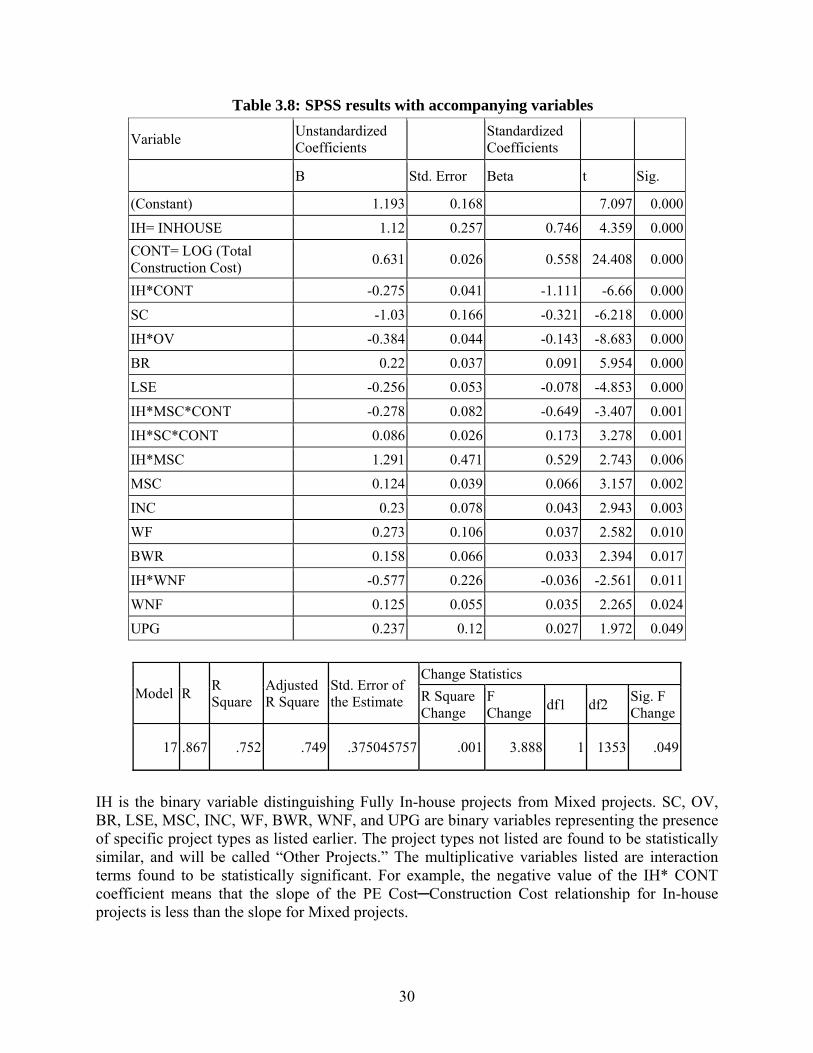
30

Table 3.8: SPSS results with accompanying variables

Variable Unstandardized Coefficients Standardized

Coefficients

B Std. Error Beta t Sig.

(Constant) 1.193 0.168 7.097 0.000

IH= INHOUSE 1.12 0.257 0.746 4.359 0.000CONT= LOG (Total Construction Cost) 0.631 0.026 0.558 24.408 0.000

IH*CONT -0.275 0.041 -1.111 -6.66 0.000

SC -1.03 0.166 -0.321 -6.218 0.000

IH*OV -0.384 0.044 -0.143 -8.683 0.000

BR 0.22 0.037 0.091 5.954 0.000

LSE -0.256 0.053 -0.078 -4.853 0.000

IH*MSC*CONT -0.278 0.082 -0.649 -3.407 0.001

IH*SC*CONT 0.086 0.026 0.173 3.278 0.001

IH*MSC 1.291 0.471 0.529 2.743 0.006

MSC 0.124 0.039 0.066 3.157 0.002

INC 0.23 0.078 0.043 2.943 0.003

WF 0.273 0.106 0.037 2.582 0.010

BWR 0.158 0.066 0.033 2.394 0.017

IH*WNF -0.577 0.226 -0.036 -2.561 0.011

WNF 0.125 0.055 0.035 2.265 0.024

UPG 0.237 0.12 0.027 1.972 0.049

Model R R Square

Adjusted R Square


Change StatisticsR Square Change

F Change df1 df2 Sig. F

Change

17 .867 .752 .749 .375045757 .001 3.888 1 1353 .049

IH is the binary variable distinguishing Fully In-house projects from Mixed projects. SC, OV, BR, LSE, MSC, INC, WF, BWR, WNF, and UPG are binary variables representing the presence of specific project types as listed earlier. The project types not listed are found to be statistically similar, and will be called “Other Projects.” The multiplicative variables listed are interaction terms found to be statistically significant. For example, the negative value of the IH* CONT coefficient means that the slope of the PE Cost─Construction Cost relationship for In-house projects is less than the slope for Mixed projects.

31

The t-values and significance of the coefficients are as listed. The Adjusted R-square of the model is 0.749, and the standard error of the estimate is 0.375. The F-significance of the model is 0.000. These numbers indicate that the model is statistically sound and explains almost 75% of the observed variance in PE charges. Therefore, it is seen that there are statistically significant differences in PE costs between Fully In-house projects and Mixed projects, and PE costs for some project types are different from the costs for others. The differences are best illustrated graphically.

3.8 Graphical Lines of Fit Figure 3.3 shows the fitted lines estimated by the model overlaid on the actual PE data for all projects, validating the postulated log-log model. The labeled lines are for the project types as listed earlier, with the lines for In-house projects labeled with an ‘In’ prefix, and those for Mixed projects with an “Mx” prefix. Each project type line is plotted only for the observed range of project construction cost for that project type and PE provider.

Figure 3.3: Total PE Costs for 1371 TxDOT Projects and Fitted Lines: Log-log Plot

To give a better sense of the numbers, the fitted lines are shown in Figure 3.4 on a standard scale. Each line is plotted only for the observed range of project construction cost for that project type.

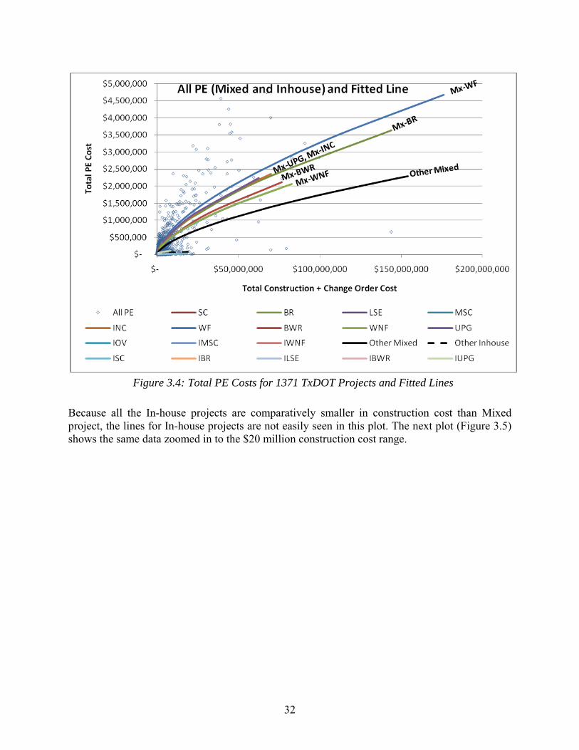
32

Figure 3.4: Total PE Costs for 1371 TxDOT Projects and Fitted Lines

Because all the In-house projects are comparatively smaller in construction cost than Mixed project, the lines for In-house projects are not easily seen in this plot. The next plot (Figure 3.5) shows the same data zoomed in to the $20 million construction cost range.

33

Figure 3.5: Total PE Costs for 1371 TxDOT Projects and Fitted Lines for In-house and Mixed

Projects: Zoomed

The graphs indicate that, as project construction cost increases, PE cost also increases, but by a diminishing amount, thus confirming economies of scale. If a letting program includes multiple small-dollar projects, it will have a higher PE cost rate than one with large projects of comparable total value. Viewed another way, PE output (dollars let per dollar PE cost) must vary depending on size and complexity of the projects being designed.

3.9 Interpretation of Results These results show that project construction cost, PE provider, and project type account for about 75% of the variance in PE costs. The differences in PE costs among project types can best be seen when the fitted lines are transformed to estimate the percentage PE, i.e., the estimated PE cost from the fitted lines are divided by actual project construction cost and expressed as a percentage. Figure 3.6 shows the plots for Mixed and In-house projects.

34

Figure 3.6: Estimation of Percentage PE Costs for Mixed and In-house Projects based on

1,371 TxDOT Projects

For all project types the percentage PE decreases as project cost increases. WF is the highest line, indicating that Widening Freeways are the most costly PE work. This project type may also include NLF—New Location Freeways and CNF─Converting Non Freeway to Freeway. Next down is UPG─Upgrading Freeways to Standards, followed by INC─Interchanges and BR─Bridge Replacement. Fairly close next are BWR─Bridge Widen/Rehab and WNF─Widen Non Freeway, with MSC- Miscellaneous Construction essentially on the same line. The next line is the pool group, labeled as “Other Mixed,” for project types not identified as statistically different from each other. For example, OV─Overlays are in the pool group. This chart can be interpreted as an indicator of the relative complexity of the various project types, with the more complex types higher up and the less complex lower down. To see In-house projects more clearly, the same data is plotted for lower contract values only (Figure 3.7). Note that the scale is different, to show more detail.

35

Figure 3.7: Estimation of Percentage PE Costs for Mixed and In-house Projects based on

1,371 TxDOT Projects: Zoomed

As before, for all project types the percentage PE decreases as project cost increases. Of Fully In-house project types, UPG─Upgrade Freeway to Standards, is the most costly, followed closed by BR─Bridge Replacement, and BWR─Bridge Widen/Rehab. Below that group is LSE─Landscape projects. Next down are MSC─Miscellaneous Construction, OV─Overlays, and WNF─Widen Non Freeways. Both In-house and Mixed SC-Seal coats are fairly close at the bottom, indicating that this is the cheapest project type. Note that there are no “In-house” lines for the most costly Mixed PE project types, namely WF, NLF, CNF, and INC, because hardly any are done Fully In-house. Table 3.9 summarizes the observed construction cost and estimated (fitted line) percentage PE by project type for Mixed and Fully In-house projects. Generally, for Fully In-house projects, the median construction cost and estimated PE percentage are lower.

36

Table 3.9: Observed Construction Cost And Estimated Percentage PE By Project Type Projects Ranges Medians Type No. Construction Cost Est. % PE Constr. Cost Est. % PE In-house BR 10 $123k-$1.748m 18.0-3.3% $472k 7.7%Mixed BR 136 $182k-$144.041m 29.7-2.5% $1.133m 15.1%In-house BWR 5 $276k-$1.849m 9.3-2.7% $384k 7.5%Mixed BWR 30 $372k-$76.821m 19.7-2.8% $2.308m 10.1%Mixed CNF 7 $22.089m-$99.785m 3.0-1.7% $38.311m 2.5%In-house INC 1 - - $18.555m 0.7%Mixed INC 26 $2.411m-$69.908m 11.7-3.4% $23.971m 5.0%In-house LSE 72 $40k-$2.826m 12.4-0.8% $250k 3.8%Mixed LSE 4 $134k-$1.126m 11.1-5.1% $208k 9.5%In-house MSC 144 $49k-$14.492m 25.2-0.1% $455k 3.2%Mixed MSC 124 $60k-$74.904m 35.8-2.6% $1.508m 10.9%Mixed NLF 1 - - $67.467m 2.0%In-house OV 116 $160k-$11.275m 3.8-0.2% $2.022m 0.7%Mixed OV 20 $134k-$9.789m 20.0-4.1% $3.136m 6.3%In-house SC 74 $396k-$18.483m 1.4-0.2% $4.790m 0.4%Mixed SC 5 $1.092m-$8.045m 0.9-0.4% $6.984m 0.4%In-house UPG 5 $718k-$8.331m 6.0-1.2% $5.700m 1.6%Mixed UPG 5 $3.489m-$62.416m 10.4-3.6% $14.774m 6.1%In-house WF 1 - - $394k 9.6%Mixed WF 13 $4.144m-$176.140m 10.6-2.7% $59.365m 4.0%In-house WNF 3 $2.395m-$8.023m 0.6-0.3% $2.704m 0.5%Mixed WNF 59 $1.552m-$82.910m 10.8-2.5% $13.668m 4.8%Other In-house 285 $29k-$22.425m 27.6-0.4% $776m 2.7%Other Mixed 327 $58k-$154.257m 27.2-1.5% $3.390m 6.1%

If project construction cost is a proxy for project scope, then Fully In-house projects are smaller in scope than Mixed projects. As seen earlier, the more complex project types are rarely done In-house. Thus, the portfolio of Mixed projects is different from Fully In-house in scope and complexity. In that case, a gross PE percentage comparison is simplistic and misleading, and caution should be exercised in interpreting such numbers from any DOT. Clearly, gross percentage PE depends on the mix of project types and project costs, aside from PE provider. However, in this dataset, for those project types done Fully In-house or Mixed, the statistically estimated percentage PE is always less for In-house projects than for Mixed projects, as illustrated in the graphs. This finding must be qualified with some caveats. Project type and construction cost are not the only measures of PE needs: two projects of the same type and equal construction cost may have entirely different PE requirements. The fact that a project required consultant PE suggests that the in-house staff, for whatever reason, could not do the work. Finally, this analysis uses PE cost data recorded by TxDOT. The timing of this work did not allow for examination of the accuracy of the PE charges recorded for projects.

37

3.10 Direct Comparison of In-house and Consultant PE Costs This section presents a comparison of PE costs for In-house and Consultant work at the function code level. In the previously presented Project Type analyses, it was found that In-house projects have lower PE costs than Mixed projects. There are no 100% Consultant projects, so it is not possible to do a direct comparison at the project level. However, since PE costs are tracked at the function code level, it is possible to find projects in which specific functions are recorded as having been done 100% In-house PE or 100% consultant PE, and to do a statistical comparison of those.

3.10.1 Function Codes with 100% Consultant Charges Table 3.10 lists those functions found to be done 100% In-house or 100% Consultant, for a number of projects.

Table 3.10: Functions that were done 100% in-house or 100% consultant Function Description Total Projects 102 Feasibility Studies 89110 Route and Design Studies 344

120 Social, Economic and Environmental Studies and Public Involvement

346

130 Right-of-Way Data (State or Contract Provided) 335150 Field Surveying and Photogrammetry 442160 Roadway Design Controls (Computations and Drafting) 631161 Drainage 454162 Signing, Pavement Markings, Signalization (Permanent) 467163 Miscellaneous (Roadway) 560170 Bridge Design 206

Functions with a small number of projects were not included, to ensure that the statistical analysis would be valid. Table 3.11 shows the total PE cost expended on these functions for the entire dataset, and the computed ‘weight’ of each function out of total PE expenditures.

38

Table 3.11: Weights of Functions Function Total PE $ Weight Construction Cost of Projects 102 1,056,099 0.26% 2,722,515,830 110 32,268,965 7.93% 6,406,203,153 120 21,668,917 5.32% 6,594,209,647 130 34,220,439 8.40% 5,728,101,105 150 53,751,613 13.20% 6,519,670,707 160 54,414,968 13.36% 6,814,693,936 161 32,873,019 8.07% 5,605,781,825 162 19,369,026 4.76% 5,745,882,565 163 75,122,028 18.45% 7,475,603,564 170 32,796,772 8.05% 4,890,816,757 Total 87.81%

Of the 29 PE functions tracked by TxDOT, the above 10 functions make up 87.81% of total preliminary engineering cost. These functions cover most of the PE cost and are thus sufficient to draw conclusions about their effects on overall PE costs.

3.10.2 Analysis and Results As before, to compare In-house PE Costs to the other group (in this case, 100% Consultant functions), stepwise regression was done. ‘In-house’ was used as the switch variable. Project Construction Cost (‘Total contract’) was also submitted to see if it had an effect on PE costs at the function level, as it was found to do at the project level. Each function was analyzed separately, and the results are summarized in Table 3.12. The detailed SPSS outputs are in Appendix A.

Table 3.12: Function Code SPSS Results

Step 1: Difference of Means Step 2: Difference when Project Cost Effect

Taken Into AccountFunc-tion

Cons-tant

In-house

Consultant/ IH Ratio

Cons-tant

In-house

Total Contract

Consultant/ IH Ratio

102 3.870 -1.180 15.14 3.870 -1.180 15.14110 3.979 -1.057 11.40 1.908 -1.062 0.334 11.53120 1.309 0 1.00 1.756 -0.498 0.350 3.15130 3.704 -0.922 8.36 2.231 -0.937 0.237 8.65150 4.356 -1.027 10.64 2.536 -1.025 0.292 10.59160 0.389 0 1.00 0.933 -0.660 0.573 4.57161 4.519 -0.788 6.14 1.022 -0.750 0.539 5.62162 0.848 0 1.00 1.178 -0.260 0.414 1.82163 0.537 0 1.00 1.018 -0.512 0.559 3.25170 4.148 -0.623 4.20 1.420 -0.583 0.415 3.83

The Step 1 portion of the table computed the difference in mean PE costs between 100% In-house work and 100% Consultant work by function code. In every case the Consultant to In-house PE cost ratio was estimated as greater than or equal to 1. Step 2 computed the difference in mean PE costs when project size (Construction Cost) is taken into account. This time, in every

39

case the Consultant to In-house PE cost ratio was estimated as greater than 1. Construction cost is significant in every case except Function 102, i.e., PE costs at the function code level are correlated with project size, increasing at a tapering rate as construction cost increases. It is clear from these results that for the same project size and the same PE function, in-house cost is less than consultant cost, by a factor that ranges from 1.82 for Function 162 (Signing) up to 15.14 for Function 102 (Feasibility Studies). Of course, project construction cost is not a true measure of project size or complexity, and it is also clear that TxDOT hired the consultants because in-house staff was not able to do the work. To compute an overall Consultant to In-house ratio of PE costs, there are multiple approaches. Here one approach is presented, for illustration purposes only. The Consultant/In-house ratios computed at Step 2 above are weighted by the percentages computed for each function in Table 3.12, to arrive at an estimated overall Consultant/In-house ratio. The computation is shown in Table 3.13.

Table 3.13: Consultant/In-house Cost Ratios

Function WeightConsultant/ In-house Ratio Effect

102 0.26% 15.14 0.0394 110 7.93% 11.53 0.9143 120 5.32% 3.15 0.1676 130 8.40% 8.65 0.7266 150 13.20% 10.59 1.3979 160 13.36% 4.57 0.6106 161 8.07% 5.62 0.4535 162 4.76% 1.82 0.0866 163 18.45% 3.25 0.5996 170 8.05% 3.83 0.3083 Other Functions 12.19% 1.00 (assumed) 0.1219 Total 100.00% 5.4265

These numbers indicate that Consultant PE is about 5.4 times as costly as In-house PE when project size (cost) is controlled for, with the caveats previously discussed. This ratio can be compared to the previously presented results of Mixed to In-house PE, namely:

• PE for the median Mixed project is 12.47 times as expensive as the median In-house project.

• PE cost increases with increasing project size, and for two projects of identical construction cost, the PE cost of a Mixed project is 7.55 times the cost of the In-house project.

• PE cost increases with increasing project size, but with different slopes and intercepts for In-house and Mixed projects. For a $1 million project, Mixed PE Cost is estimated at $115,080 compared to In-house PE Cost of $18,197, a factor of 6.32 times.

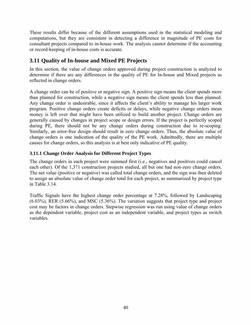
40

These results differ because of the different assumptions used in the statistical modeling and computations, but they are consistent in detecting a difference in magnitude of PE costs for consultant projects compared to in-house work. The analysis cannot determine if the accounting or record-keeping of in-house costs is accurate.

3.11 Quality of In-house and Mixed PE Projects In this section, the value of change orders approved during project construction is analyzed to determine if there are any differences in the quality of PE for In-house and Mixed projects as reflected in change orders. A change order can be of positive or negative sign. A positive sign means the client spends more than planned for construction, while a negative sign means the client spends less than planned. Any change order is undesirable, since it affects the client’s ability to manage his larger work program. Positive change orders create deficits or delays, while negative change orders mean money is left over that might have been utilized to build another project. Change orders are generally caused by changes in project scope or design errors. If the project is perfectly scoped during PE, there should not be any change orders during construction due to re-scoping. Similarly, an error-free design should result in zero change orders. Thus, the absolute value of change orders is one indication of the quality of the PE work. Admittedly, there are multiple causes for change orders, so this analysis is at best only indicative of PE quality.

3.11.1 Change Order Analysis for Different Project Types The change orders in each project were summed first (i.e., negatives and positives could cancel each other). Of the 1,371 construction projects studied, all but one had non-zero change orders. The net value (positive or negative) was called total change orders, and the sign was then deleted to assign an absolute value of change order total for each project, as summarized by project type in Table 3.14. Traffic Signals have the highest change order percentage at 7.28%, followed by Landscaping (6.03%), RER (5.66%), and MSC (5.36%). The variation suggests that project type and project cost may be factors in change orders. Stepwise regression was run using value of change orders as the dependent variable, project cost as an independent variable, and project types as switch variables.

41

Table 3.14: Absolute Value of Change Orders by Project Type Project Type Total PE Total Construction

CostAbsolute Change Order Totals

Change Orders as % of Constr.

BCF $173,264 $4,340,402 $5,236 0.12%BR $36,560,781 $492,979,632 $9,092,843 1.84%BWR $13,486,429 $180,245,906 $5,099,409 2.83%CNF $17,424,537 $302,483,400 $2,825,932 0.93%CTM $2,009,864 $60,663,608 $592,463 0.98%FBO $1,708,164 $22,512,000 $0 0.00%HES $473,632 $3,966,527 $102,876 2.59%INC $46,566,058 $767,225,316 $18,903,151 2.46%LSE $1,066,817 $32,958,958 $1,986,869 6.03%MSC $53,083,978 $664,266,148 $35,583,165 5.36%NLF $4,747,721 $67,299,167 $167,762 0.25%NNF $10,052,820 $185,533,411 $2,872,430 1.55%OV $6,482,558 $399,070,320 $17,264,115 4.33%RER $35,405,718 $681,251,748 $38,536,959 5.66%RES $4,727,968 $125,500,828 $4,819,650 3.84%ROW $7,673,516 $144,225,877 $1,947,949 1.35%SC $1,741,610 $427,983,182 $11,583,735 2.71%SFT $49,055,353 $906,037,924 $30,974,791 3.42%SRA $3,556,839 $42,035,563 $0 0.00%TC $117,895 $165,510 $0 0.00%TPD $70,125 $7,156,452 $236,737 3.31%TS $2,682,635 $25,316,440 $1,842,385 7.28%UGN $3,556,812 $53,526,170 $2,498,003 4.67%UPG $5,976,360 $135,998,603 $1,633,240 1.20%WF $37,795,068 $818,646,592 $8,291,332 1.01%WNF $60,794,086 $1,001,017,297 $22,529,231 2.25%

3.11.2 Change Order Analysis Results As before, log transformation of the data was done. Change orders which were less than $1 were changed to $1 for this purpose. Table 3.15 presents the SPSS results at the final step.

42

Table 3.15: SPSS results with change order analysis Model Summary

Model R R Square

Adjusted R Square


Change Statistics R Square Change


Change

9 .488 .238 .233 1.543355970 .002 4.162 1 1361 .042

Coefficients

Model Unstandardized Coefficients Standardized

Coefficients t Sig. B Std. Error Beta

9

(Constant) -3.446 .433 -7.961 .000Contract Amount 1.203 .068 .455 17.620 .000SRA -5.117 .895 -.136 -5.719 .000FBO -5.398 1.546 -.083 -3.491 .000BR -.406 .141 -.071 -2.874 .004SC -.539 .185 -.071 -2.917 .004I*LSE .542 .200 .069 2.705 .007I*SFT -.613 .199 -.089 -3.078 .002SFT .350 .133 .078 2.629 .009RER .311 .152 .051 2.040 .042

a. Dependent Variable: Absolute Change Order The final model has an R-squared value of 0.238, a relatively low number, meaning the model may not adequately estimate change orders. There is no general coefficient for In-house projects, meaning there is no significant difference in change orders between In-house and Mixed projects. However, some project types are found to differ significantly from the norm. The B coefficients indicate the effect of the significant variables. The 1.203 coefficient (>1) for Contract Amount indicates that, as project construction cost increases, change orders increase at a faster rate. This suggests that larger or more complex projects are likely to see a higher rate of change orders. The negative coefficients for some project types indicate that those are likely to have fewer change orders. Among projects with Mixed PE, Ferry Boat (FBO) and Safety Rest Area (SRA) are likely to have the least change orders. Seal Coat (SC) and Bridge Replacement (BR) with Mixed PE also have lower than average change orders, while Mixed PE Rehabilitation of Existing Roads (RER) and Safety Projects (SFT) have higher than average change orders. Two In-house PE project types differ from the norm: Landscape and Scenic Project (LSE) have higher change order rates, while Safety Projects (SFT) are lower. Essentially, change orders relate more to project type than to PE provider.

43

The following charts illustrate the results. Figure 3.8 is absolute change order versus contract amount on a log-log scale with raw data and fitted lines of the project types found to be significantly different from the norm. Figure 3.9 is the same data on a normal scale, and Figure 3.10 is a normal scale chart of the same data but only for smaller contract amounts.

Figure 3.8: Total Change Orders and Fitted Lines: Log-log Plot

0

1

2

3

4

5

6

7

8

4 4.5 5 5.5 6 6.5 7 7.5 8 8.5

Abs

olut

e Ch

ange

Ord

er

Contract Amount

Change Order for different Project Types (log-Log)

Change Order BR SC In-LSE In-SFT SFT RER Other

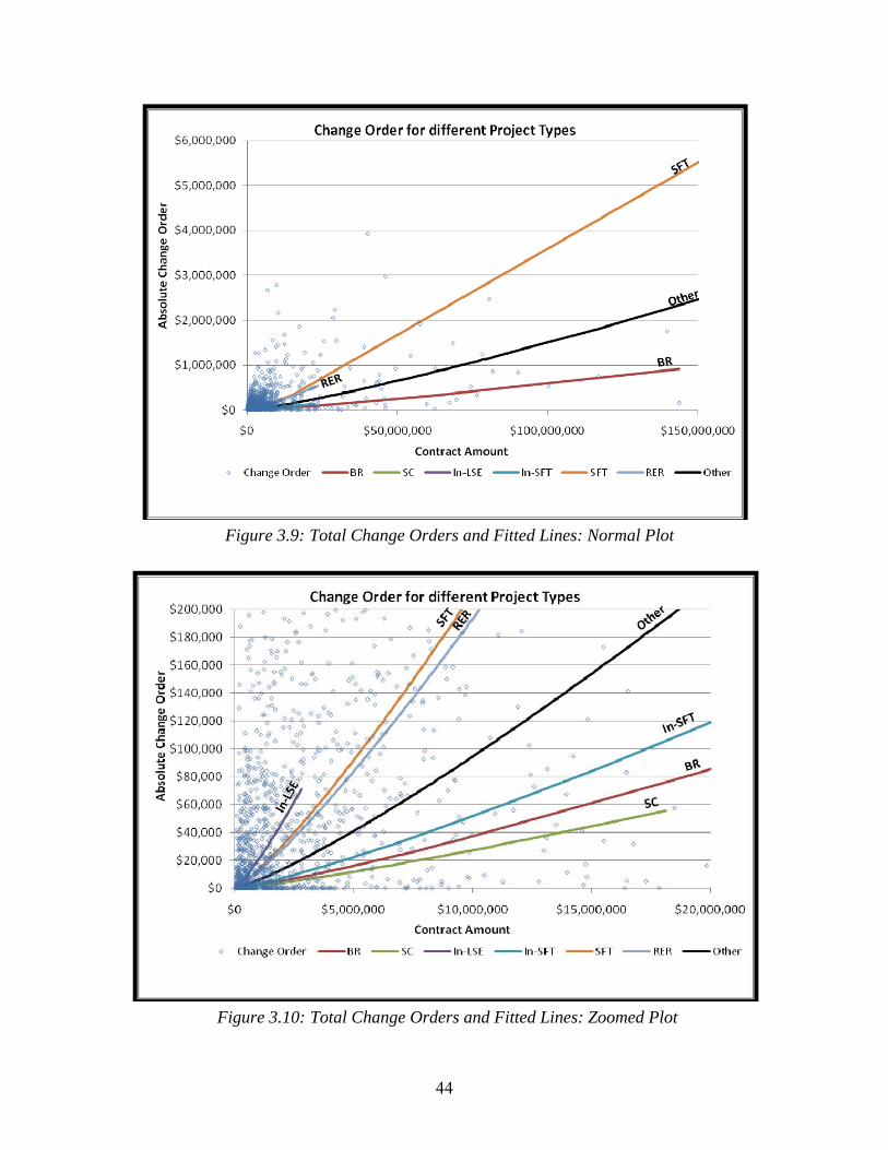
44

Figure 3.9: Total Change Orders and Fitted Lines: Normal Plot

Figure 3.10: Total Change Orders and Fitted Lines: Zoomed Plot

45

The charts confirm that change order rates for in-house projects span the same spectrum as those for mixed projects. Project type is the most significant factor in change order rate. Overall, consultant involvement seems to make no difference in the rate of change orders, and by extension, the quality, and completeness of PE for different project types. The percentage change order versus total contract amount for selected project types is plotted in Figures 3.11 and 3.12.

Figure 3.11: Estimated Change Order Percentage by Project Type

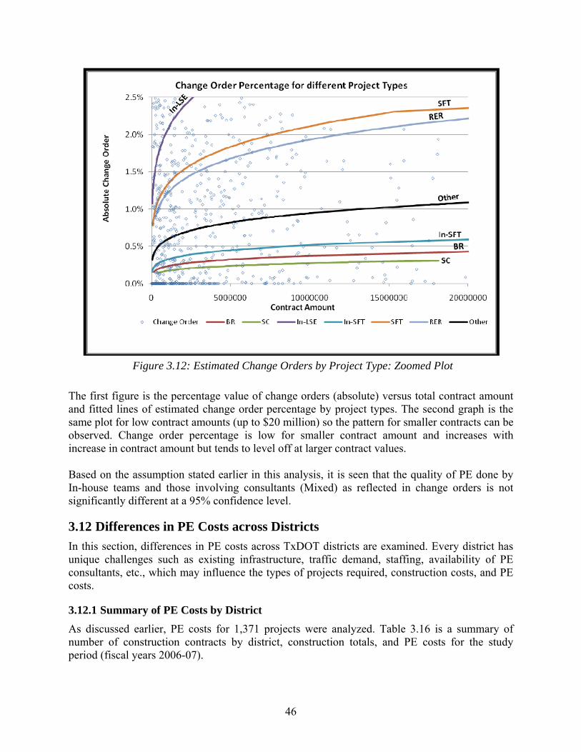
46

Figure 3.12: Estimated Change Orders by Project Type: Zoomed Plot

The first figure is the percentage value of change orders (absolute) versus total contract amount and fitted lines of estimated change order percentage by project types. The second graph is the same plot for low contract amounts (up to $20 million) so the pattern for smaller contracts can be observed. Change order percentage is low for smaller contract amount and increases with increase in contract amount but tends to level off at larger contract values. Based on the assumption stated earlier in this analysis, it is seen that the quality of PE done by In-house teams and those involving consultants (Mixed) as reflected in change orders is not significantly different at a 95% confidence level.

3.12 Differences in PE Costs across Districts In this section, differences in PE costs across TxDOT districts are examined. Every district has unique challenges such as existing infrastructure, traffic demand, staffing, availability of PE consultants, etc., which may influence the types of projects required, construction costs, and PE costs.

3.12.1 Summary of PE Costs by District As discussed earlier, PE costs for 1,371 projects were analyzed. Table 3.16 is a summary of number of construction contracts by district, construction totals, and PE costs for the study period (fiscal years 2006-07).

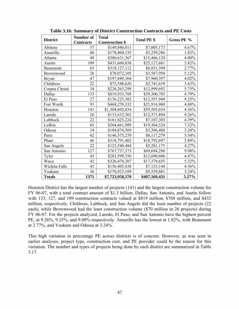
47

Table 3.16: Summary of District Construction Contracts and PE Costs

District Number of Contracts

Total Construction $ Total PE $ Gross PE %

Abilene 37 $149,846,011 $7,005,173 4.67%Amarillo 40 $178,804,155 $3,259,286 1.82%Atlanta 49 $386,631,367 $15,466,124 4.00%Austin 109 $431,660,038 $25,127,681 5.82%Beaumont 63 $319,127,112 $8,831,399 2.77%Brownwood 26 $70,072,105 $3,587,950 5.12%Bryan 47 $197,849,364 $7,960,397 4.02%Childress 22 $75,548,620 $2,741,639 3.63%Corpus Christi 34 $226,263,299 $12,999,692 5.75%Dallas 133 $819,933,768 $39,300,785 4.79%El Paso 27 $136,225,382 $12,597,949 9.25%Fort Worth 93 $468,270,332 $21,916,960 4.68%Houston 141 $1,304,692,034 $59,505,654 4.56%Laredo 26 $133,632,362 $12,371,894 9.26%Lubbock 22 $161,825,224 $7,107,303 4.39%Lufkin 65 $264,661,989 $19,364,324 7.32%Odessa 34 $104,874,569 $3,396,488 3.24%Paris 42 $146,575,270 $8,117,279 5.54%Pharr 46 $318,791,402 $18,792,697 5.89%San Angelo 22 $123,540,484 $5,281,175 4.27%San Antonio 127 $767,737,373 $69,694,296 9.08%Tyler 43 $283,599,356 $12,690,606 4.47%Waco 42 $326,470,207 $17,379,655 5.32%Wichita Falls 45 $156,403,438 $7,133,144 4.56%Yoakum 36 $170,923,109 $5,539,881 3.24%Totals 1371 $7,723,958,370 $407,169,431 5.27%

Houston District has the largest number of projects (141) and the largest construction volume for FY 06-07, with a total contract amount of $1.3 billion. Dallas, San Antonio, and Austin follow with 133, 127, and 109 construction contracts valued at $819 million, $768 million, and $432 million, respectively. Childress, Lubbock, and San Angelo did the least number of projects (22 each), while Brownwood had the least construction volume ($70 million in 26 projects) during FY 06-07. For the projects analyzed, Laredo, El Paso, and San Antonio have the highest percent PE, at 9.26%, 9.25%, and 9.08% respectively. Amarillo has the lowest at 1.82%, with Beaumont at 2.77%, and Yoakum and Odessa at 3.24%. This high variation in percentage PE across districts is of concern. However, as was seen in earlier analyses, project type, construction cost, and PE provider could be the reason for this variation. The number and types of projects being done by each district are summarized in Table 3.17.

48

Table 3.17: Summary of District Project Types and Numbers

Most districts did BR, LSE, MSC, OV, RER, SC and SFT projects. Very few did CNF, CTM, FBO, HES, NLF, NNF, ROW, SRA, TC, TPD, UGN, UPG and WF projects. Certain types of projects may be driving up some district PE costs. However, there is no obvious indication from the mix of projects as to why Laredo, El Paso, and San Antonio have a high PE percentage. The mix of in-house and consultant work in each district is also of interest. Table 3.18 is a summary of that data for projects let in FY 06-07.

Dis

tric

t

Abi

lene

Am

arill

o

Atla

nta

Aus

tin

Bea

umon

t

Bro

wnw

ood

Bry

an

Chi

ldre

ss

Corp

us C

hris

ti

Dal

las

El P

aso

Fort

Wor

th

Hou

ston

Lare

do

Lubb

ock

Lufk

in

Ode

ssa

Pari

s

Phar

r

San

Ang

elo

San

Ant

onio

Tyle

r

Wac

o

Wic

hita

Fal

ls

Yoa

kum

BCF 1BR 6 1 9 14 9 2 5 3 4 13 20 7 3 8 1 4 3 1 7 4 4 12 7BWR 5 3 1 1 1 5 2 1 1 1 8 2 1 2CNF 1 1 1 1 2 1CTM 1 1 6 5FBO 1HES 2INC 1 1 4 1 2 9 2 1 1 3 1 1LSE 4 2 1 3 1 1 16 1 2 15 1 3 2 1 3 1 9 2 2 4 2MSC 3 13 6 24 12 7 6 5 2 37 13 19 45 6 5 5 6 3 3 4 23 10 5 5 1NLF 1NNF 1 1 2 2 1 1 1OV 7 12 2 19 12 2 1 2 4 4 1 3 20 3 1 4 3 2 2 2 13 5 1 9 2RER 5 6 2 3 7 6 4 6 4 9 1 3 8 3 4 6 3 4 1 6 19 3 4 5 2RES 2 9 5 2 1 2 2 1 2 3 3 7ROW 1 1SC 4 2 3 6 2 2 3 2 3 5 1 2 2 5 4 3 7 2 3 5 2 5 2 4SFT 2 2 22 34 14 16 3 8 14 2 23 8 5 2 27 6 13 9 21 9 12 5 6SRA 1 1 1TC 1TPD 2TS 2 2 12 7 2 1 4 3 1 2 5 1UGN 1 1 2 1 1 1 1UPG 4 4 1 2 1WF 1 3 2 5 1 1 1WNF 2 1 1 1 1 1 7 3 8 3 16 7 5 1 1 2Totals 37 40 49 109 63 26 47 22 34 133 27 93 141 26 22 65 34 42 46 22 127 43 42 45 36

49

Table 3.18: Data for projects let in FY 06-07

District

In-house Projects Mixed Projects

No. of Pro-jects

Construction $

PE Spending

Mean PE%

No. of Pro-jects

Construction $

PE Spending

Mean PE%

Abilene 20 54,364,324 751,259 1.4% 17 95,481,687 6,253,914 6.5%

Amarillo 30 87,647,360 591,523 0.7% 10 91,156,796 2,667,763 2.9%

Atlanta 25 75,847,022 793,376 1.0% 24 310,784,345 14,672,749 4.7%

Austin 41 67,089,846 694,465 1.0% 68 364,570,192 24,433,216 6.7%

Beaumont 32 69,418,805 764,986 1.1% 31 249,708,306 8,066,413 3.2%

Brownwood 18 27,104,825 712,428 2.6% 8 42,967,280 2,875,522 6.7%

Bryan 31 52,288,738 1,001,074 1.9% 16 145,560,626 6,959,323 4.8%

Childress 10 26,678,658 163,137 0.6% 12 48,869,962 2,578,502 5.3%

Corpus Christi 13 40,065,345 589,317 1.5% 21 186,197,954 12,410,375 6.7%

Dallas 44 77,212,112 1,005,438 1.3% 89 742,721,657 38,295,347 5.2%

El Paso 10 29,142,435 362,178 1.2% 17 107,082,947 12,235,771 11.4%

Fort Worth 32 68,877,569 869,514 1.3% 61 399,392,763 21,047,446 5.3%

Houston 77 164,717,748 3,267,078 2.0% 64 1,139,974,285 56,238,576 4.9%

Laredo 5 7,012,167 41,847 0.6% 21 126,620,195 12,330,047 9.7%

Lubbock 14 59,586,810 502,768 0.8% 8 102,238,414 6,604,535 6.5%

Lufkin 26 36,473,261 530,097 1.5% 39 228,188,728 18,834,228 8.3%

Odessa 31 75,867,340 1,154,977 1.5% 3 29,007,229 2,241,511 7.7%

Paris 20 46,093,842 652,336 1.4% 22 100,481,428 7,464,944 7.4%

Pharr 18 39,190,907 547,991 1.4% 28 279,600,495 18,244,706 6.5%

San Angelo 15 47,215,288 713,667 1.5% 7 76,325,196 4,567,508 6.0%

San Antonio 34 61,778,687 1,081,211 1.8% 93 705,958,686 68,613,085 9.7%

Tyler 23 106,394,558 751,559 0.7% 20 177,204,798 11,939,047 6.7%

Waco 17 38,587,663 542,559 1.4% 25 287,882,544 16,837,096 5.8%

Wichita Falls 24 67,271,141 472,907 0.7% 21 89,132,297 6,660,237 7.5%

Yoakum 12 35,942,957 236,590 0.7% 24 134,980,152 5,303,290 3.9%

Odessa (91%) had the highest percentage of In-house projects followed by Amarillo (75%) and Brownwood (69%) while Laredo (81%) has done the highest percentage of Mixed projects followed by San Antonio (27%) and Dallas (33%). In every case the mean PE percentage for Mixed projects is far higher than that for In-house projects. Looking specifically at Laredo, El Paso, and San Antonio, it is seen that these districts have the highest Mixed PE percentage, but their In-house percentage is normal.

50

3.12.2 Simple Comparison of Districts In this analysis at the district level, PE costs are estimated as functions of project construction cost. District is introduced as a switch variable to allow comparisons across districts. Table 3.19 presents the final SPSS result.

Table 3.19: SPSS results of simple comparison of districts

Coefficients



B Std. Error Beta 10 (Constant) .451 .148 3.052 .002

Total Contract Amount .691 .023 .611 29.469 .000

San Antonio .379 .055 .147 6.929 .000 Amarillo -.359 .092 -.081 -3.888 .000 Fort Worth .235 .063 .079 3.744 .000 El Paso .316 .112 .059 2.836 .005 Dallas .162 .053 .064 3.029 .003 Laredo .305 .114 .056 2.687 .007 Pharr .203 .087 .049 2.345 .019 Lufkin .154 .074 .044 2.097 .036 Waco .188 .090 .043 2.079 .038

Model R R Square

Adjusted R Square


Change Statistics R Square Change

F Change

df1 df2

Sig. F Change

10 .651 .424 .420 .5697475 .002 4.323 1 1360 .038 The model shown has an adjusted R-squared value of 0.420, a reasonable number, meaning the model adequately estimates differences across districts. The B coefficients indicate the effect of the significant variables. The 0.691 coefficient for Contract Amount indicates that, as project construction cost increases, PE cost increases at a tapering rate. The districts not shown are the statistically selected pool (not necessarily the average districts). Eight districts have PE costs above the pool. When the effect of Contract Amount (project size) is separated, San Antonio has the highest PE costs at 2.39 times the pool, followed by El Paso at 2.07, Laredo at 2.02, Fort Worth at 1.72, Pharr at 1.60, Waco at 1.54, Dallas at 1.45, and Lufkin at 1.43. Amarillo is lower than the pool, at 0.44 times the remaining districts.

3.12.3 Comparison of Districts Considering PE Provider

Previous analysis found that PE costs are a function of PE provider (In-house or Mixed). In this section, PE provider and district are introduced to determine whether the differences in PE costs across districts are due to the choice of PE provider.

51

As before, PE cost is the dependent variable while project construction cost and the interaction variable for provider and project cost were selected as continuous independent variables. Switch variables were District, Provider, and the interaction term for district and provider. Following in Table 3.20 are the SPSS results of this analysis.

Table 3.20: SPSS results of district comparisons considering PE provider



B Std. Error Beta

13

(Constant) 1.211 .149 8.140 .000In-house 1.458 .218 .971 6.699 .000Total Contract Amount .639 .023 .565 27.919 .000

IH*CONTRACT -.365 .035 -1.474 -10.489 .000San Antonio .143 .037 .056 3.877 .000In*Austin*Cont -.051 .011 -.068 -4.708 .000Amarillo -.238 .064 -.054 -3.749 .000In*Childress*Cont -.066 .021 -.045 -3.129 .002Yoakum -.190 .066 -.041 -2.857 .004In*Wichita Falls*Cont -.038 .013 -.041 -2.832 .005

In*Lufkin*Cont -.501 .136 -.533 -3.685 .000In*Lufkin 2.716 .793 .495 3.424 .001In*Laredo*Cont -.080 .029 -.039 -2.762 .006El Paso .183 .076 .034 2.396 .017

Model Summary

Model R R Square

Adjusted R Square



F Change

df1 df2 Sig. F

Change13 .854 .729 .726 .3915863 .001 5.739 1 1357 .017

In the table, an ‘In’ or ‘IH’ prefix indicates in-house projects for that district (different intercepts) and the ‘Cont’ suffix indicates interaction with total contract amount (different PE-construction cost slopes). The final model has an adjusted R-squared value of 0.726, a large number, meaning the model strongly estimates PE costs. However, comparing this figure to the R-square value of 0.420 for districts only, it is clear that PE provider is a major factor in PE costs across all districts. The B coefficients are listed in order of entry into the model. For example, the switch variable In-house entered first, indicating that PE provider is the strongest indicator of differences in PE costs. Next, Total Contract Amount (project construction cost) entered, saying that project size is the next strongest factor in PE costs. Finally, the interaction variable IH*Contract entered, indicating that there are major differences in the sizes of projects done In-house versus Mixed. Then District variables began to enter.

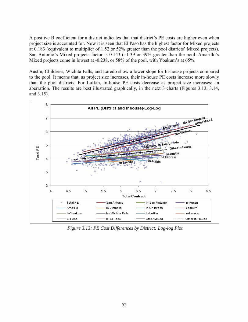
52

A positive B coefficient for a district indicates that that district’s PE costs are higher even when project size is accounted for. Now it is seen that El Paso has the highest factor for Mixed projects at 0.183 (equivalent to multiplier of 1.52 or 52% greater than the pool districts’ Mixed projects). San Antonio’s Mixed projects factor is 0.143 (=1.39 or 39% greater than the pool. Amarillo’s Mixed projects come in lowest at -0.238, or 58% of the pool, with Yoakum’s at 65%. Austin, Childress, Wichita Falls, and Laredo show a lower slope for In-house projects compared to the pool. It means that, as project size increases, their in-house PE costs increase more slowly than the pool districts. For Lufkin, In-house PE costs decrease as project size increases; an aberration. The results are best illustrated graphically, in the next 3 charts (Figures 3.13, 3.14, and 3.15).

Figure 3.13: PE Cost Differences by District: Log-log Plot

53

Figure 3.14: PE Cost Differences by District: Normal Plot

Figure 3.15: PE Cost Differences by District: Zoomed Plot

54

In every district, In-house projects have less PE cost than mixed projects for the usual range of project size, consistent with the results of previous analyses. All districts have fairly similar In-house PE costs that increase with project size. However, there are large differences in the costs of Mixed projects across districts, with El Paso, San Antonio, and Bryan being higher than average, and Amarillo, Yoakum, and Beaumont being lower than average.

3.12.4 Comparison of Districts by PE Provider and Project Type Earlier analyses showed that project type is an important factor in predicting PE costs both for In-house and Mixed projects. In this section, project type is introduced along with district and PE provider as switch variables. As before, PE cost is the dependent variable, project construction cost in the continuous independent variable, and interaction terms among the predictor variables are also tested. The SPSS results are presented in Table 3.21.

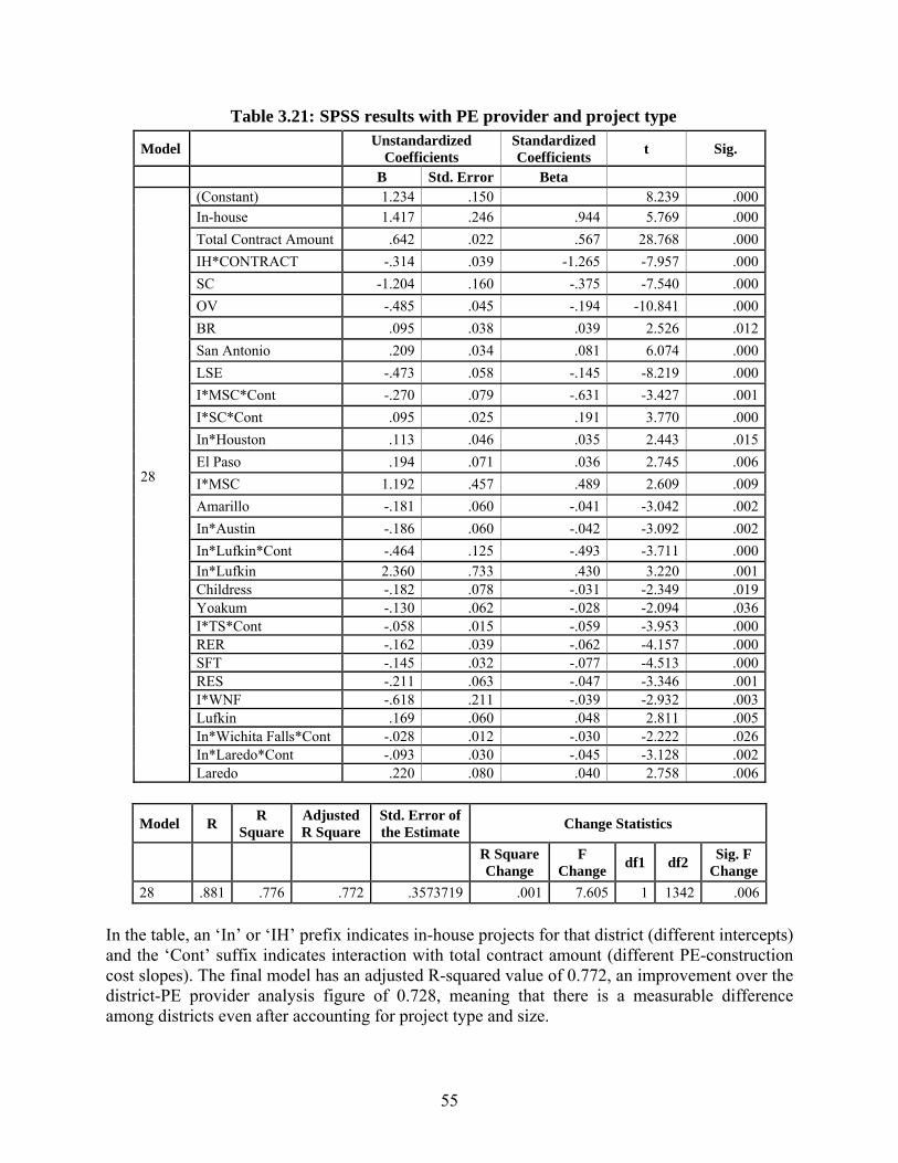
55

Table 3.21: SPSS results with PE provider and project type



B Std. Error Beta

28

(Constant) 1.234 .150 8.239 .000In-house 1.417 .246 .944 5.769 .000Total Contract Amount .642 .022 .567 28.768 .000IH*CONTRACT -.314 .039 -1.265 -7.957 .000SC -1.204 .160 -.375 -7.540 .000OV -.485 .045 -.194 -10.841 .000BR .095 .038 .039 2.526 .012San Antonio .209 .034 .081 6.074 .000LSE -.473 .058 -.145 -8.219 .000I*MSC*Cont -.270 .079 -.631 -3.427 .001I*SC*Cont .095 .025 .191 3.770 .000In*Houston .113 .046 .035 2.443 .015El Paso .194 .071 .036 2.745 .006I*MSC 1.192 .457 .489 2.609 .009Amarillo -.181 .060 -.041 -3.042 .002In*Austin -.186 .060 -.042 -3.092 .002In*Lufkin*Cont -.464 .125 -.493 -3.711 .000In*Lufkin 2.360 .733 .430 3.220 .001Childress -.182 .078 -.031 -2.349 .019Yoakum -.130 .062 -.028 -2.094 .036I*TS*Cont -.058 .015 -.059 -3.953 .000RER -.162 .039 -.062 -4.157 .000SFT -.145 .032 -.077 -4.513 .000RES -.211 .063 -.047 -3.346 .001I*WNF -.618 .211 -.039 -2.932 .003Lufkin .169 .060 .048 2.811 .005In*Wichita Falls*Cont -.028 .012 -.030 -2.222 .026In*Laredo*Cont -.093 .030 -.045 -3.128 .002Laredo .220 .080 .040 2.758 .006

Model R R Square

Adjusted R Square

Std. Error of the Estimate Change Statistics

R Square Change


Change 28 .881 .776 .772 .3573719 .001 7.605 1 1342 .006

In the table, an ‘In’ or ‘IH’ prefix indicates in-house projects for that district (different intercepts) and the ‘Cont’ suffix indicates interaction with total contract amount (different PE-construction cost slopes). The final model has an adjusted R-squared value of 0.772, an improvement over the district-PE provider analysis figure of 0.728, meaning that there is a measurable difference among districts even after accounting for project type and size.

56

The B coefficients are listed in order of entry into the model. As before, the switch variable In-house entered first, indicating that PE provider is the strongest indicator of differences in PE costs. Next, Total Contract Amount (project construction cost) is entered, indicating that project size is the next strongest factor in PE costs. The interaction variable IH*Contract is then entered, indicating that there are major differences in the sizes of projects done In-house versus Mixed. Then, three Mixed project types (SC, OV, and BR) are entered, indicating that these project types have different costs compared to other project types across all districts. A positive B coefficient for a district indicates that its PE costs are higher even when PE provider, project type, and size are accounted for. Laredo has the highest factor for Mixed projects at 0.22 (equivalent to multiplier of 1.66 or 66% greater than the pool districts’ Mixed projects). San Antonio’s Mixed projects factor is 0.209 (=1.62 or 62% greater than the pool), and El Paso’s Mixed projects factor is 0.194 (1.56 or 56% greater than the pool). Childress and Amarillo’s Mixed projects come in lowest at -0.182, or 66% of the pool, with Yoakum’s at 74%. Houston has an intercept higher than the pool for in-house projects, meaning that its in-house costs are somewhat above typical (130% of pool), while Austin has an intercept lower (65% of pool). Wichita Falls and Laredo have slopes slightly lower than the pool for in-house work, meaning their in-house PE costs do not increase as quickly as other districts when project size increases. Lufkin displays unusual behavior, with PE costs decreasing as project size increases, perhaps due to the influence of a few unusual projects. This analysis verifies that in-house projects have less PE cost than mixed projects for the usual range of project size across all districts and all project types. Most districts have fairly similar in-house PE costs that increase with project size. However, there are large differences in the costs of Mixed projects across districts, with Laredo, San Antonio, and El Paso being higher than average, and Childress, Amarillo, and Yoakum being lower than average. The reasons for the differences across districts are not clear. Perhaps they have a higher involvement of historically underutilized consultants, but that data was not available for this analysis.

3.12.5 Change Orders in Districts In this section, differences in change order rates across districts are analyzed to determine if any districts have unusual levels of change orders.

3.12.6 Change Order Rates As before, the net value of change orders was computed for each project, and the sign was deleted to create an absolute value. The totals of absolute change orders for each district are shown in Table 3.22. Laredo has the highest change order rate at 7.43%, followed by Childress and Austin. Yoakum has the lowest rate at 1.28%, followed by Wichita Falls and Paris.

57

Table 3.22: Summary of District Change Orders

District Contract Amount Absolute Change Orders

Percentage Change Orders

Abilene $146,674,578 $3,782,458 2.58% Amarillo $174,104,715 $4,967,967 2.85% Atlanta $382,089,574 $8,290,990 2.17% Austin $409,878,723 $22,612,635 5.52% Beaumont $314,138,802 $10,865,128 3.46% Brownwood $68,716,323 $1,390,456 2.02% Bryan $196,901,400 $3,518,140 1.79% Childress $71,580,027 $3,968,594 5.54% Corpus Christi $222,331,836 $4,148,136 1.87% Dallas $781,314,898 $40,099,985 5.13% El Paso $136,180,179 $4,304,108 3.16% Fort Worth $459,070,345 $15,231,286 3.32% Houston $1,288,364,624 $21,065,924 1.64% Laredo $125,403,926 $9,321,739 7.43% Lubbock $158,702,539 $3,657,547 2.30% Lufkin $258,520,074 $7,495,187 2.90% Odessa $104,301,316 $2,567,504 2.46% Paris $145,063,504 $2,133,260 1.47% Pharr $314,257,079 $5,370,686 1.71% San Angelo $123,859,762 $4,464,287 3.60% San Antonio $746,772,641 $23,912,983 3.20% Tyler $279,450,741 $5,025,190 1.80% Waco $321,804,259 $6,750,265 2.10% Wichita Falls $155,142,641 $2,280,269 1.47% Yoakum $169,595,813 $2,165,540 1.28% Totals $7,554,220,319 $219,390,264 2.90%

3.12.7 Comparison of Change Orders Across Districts For analysis, absolute values of change orders for each project were chosen as the dependent variable. ‘In-house’ and ‘District’ were used as switch variables. Project construction cost (‘contract amount’) and interactions with In-house and district are the continuous independent variables. Stepwise regression was run as before, and the SPSS results are shown in Table 3.23.

58

Table 3.23: SPSS results of change order comparisons Coefficients



B Std. Error Beta

15

(Constant) -3.284 .405 -8.107 .000

Contract Amount 1.198 .064 .453 18.713 .000Wichita Falls -1.755 .333 -.177 -5.267 .000In*Paris*Cont -.259 .056 -.108 -4.630 .000Yoakum -1.064 .258 -.097 -4.124 .000Pharr -.913 .230 -.093 -3.971 .000Corpus Christi -.960 .265 -.085 -3.619 .000In*Childress -1.484 .483 -.072 -3.069 .002In*Dallas .711 .236 .071 3.016 .003Laredo .817 .302 .063 2.705 .007Lubbock -.815 .328 -.058 -2.486 .013In*Houston 4.536 2.112 .593 2.148 .032In*Wichita Falls*Cont .165 .074 .075 2.228 .026Odessa -.569 .266 -.050 -2.138 .033Bryan -.455 .227 -.047 -1.999 .046In*Houston*Cont -.693 .351 -.545 -1.976 .048

Model Summary

Model R R Square

Adjusted R Square




Change

15 .515 .265 .257 1.51877468 .002 3.904 1 1355 .048 In the table, an ‘In’ prefix indicates In-house projects for that district (different intercepts) and the ‘Cont’ suffix indicates interaction with total contract amount (different PE-construction cost slopes). The final model has an R-squared value of 0.257, a small number, meaning the model is not a strong estimator of PE costs. However, it does find that there are statistically significant differences in change orders for some districts compared to others. The B coefficients are listed in order of entry into the model. For example, Contract Amount (project construction cost) is entered first, indicating that project size is the strongest factor in change orders. Then District variables began to enter. The B coefficient for Contract Amount is 1.198, indicating that, as project size increases, change orders increase at a faster rate. There is no B coefficient for In-house, indicating that there is no

59

statewide difference in change order rates for in-house projects versus Mixed projects. However, there are differences among districts. For Mixed projects, Laredo has a rate of 6.56 times the pool (i.e., districts not named here). Several districts are far below the pool: Wichita Falls being the lowest at 0.018 times the pool, Yoakum at 0.086, Corpus Christi at 0.11, Pharr at 0.122, Lubbock at 0.153, Odessa at 0.27, and Bryan at 0.351. For in-house projects, the picture is more muddled. Only Childress stands out on the low side, being at 0.033 times the pool. Dallas stands out on the high side, being at 5.14 times the pool, and with a higher slope even than for Mixed projects. As Dallas’ project size increases, change orders for in-house projects increase at a faster rate than for Mixed projects, and for other districts. Wichita Falls ‘compensates’ for its Mixed projects by having a similar steeper rate as Dallas for in-house projects. Paris and Houston have flatter slopes than the pool for in-house projects. Figures 3.16, 3.17, and 3.18 show these results graphically. Percentage change orders by district are shown in Figures 3.19 and 3.20.

Figure 3.16: Absolute Change Orders by District: Log-log Plot

60

Figure 3.17: Absolute Change Orders by District: Normal Plot

Figure 3.18: Absolute Change Orders by District: Zoomed Plot

61

Figure 3.19: Percentage Change Orders by District: All Projects

Figure 3.20: Percentage Change Orders by District: Projects Less Than $20 million

62

This analysis shows that most of the districts (18 out of 25) have similar change order rates for In-house and Mixed projects. The remaining 7 districts have different results, perhaps due to unique project conditions. Overall, it is seen that quality of preliminary engineering done by in-house and mixed teams, as measured by absolute value of change orders, is not significantly different across districts.

3.13 CE Results

3.13.1 Difference in CE cost by Project Types This section presents the results of a statistical analysis of Construction Engineering (CE) costs in TxDOT. A stepwise regression analysis in the SPSS statistical analysis program for CE charges on 731 projects produced the following equation:

Log (Total CE Cost) = 0.314 + 0.737 Log (CONT) + 0.269 TS + 0.134 BR + 0.112 LSE – 0.157 OV – 0.214 SC

Coefficient table and model summary of SPSS results are shown in Table 3.24.

Table 3.24: Coefficient table and model summary of SPSS results

Coefficients

7 (Constant) .314 .108 2.899 .004

Total Contract .737 .018 .943 40.786 .000

OV -.157 .026 -.127 -6.150 .000

SC -.214 .033 -.138 -6.448 .000

TS .269 .055 .099 4.903 .000

BR .134 .030 .088 4.393 .000

LSE .112 .040 .060 2.840 .005

IBWRCONT .036 .014 .049 2.515 .012

Model R R

Square Adjusted R Square


Change Statistics

R Square Change F Change df1 df2

Sig. F Change

1 .823 .677 .677 .252544708 .677 1528.961 1 729 .000

2 .831 .690 .690 .247483054 .013 31.125 1 728 .000

3 .842 .708 .707 .240330625 .018 44.977 1 727 .000

4 .846 .715 .714 .237707459 .007 17.134 1 726 .000

5 .849 .721 .719 .235403239 .006 15.282 1 725 .000

6 .851 .724 .722 .234367373 .003 7.423 1 724 .007

7 .852 .726 .724 .233509923 .002 6.327 1 723 .012

63

CONT is the total construction cost plus change orders, and Log is the base 10 logarithm of the numbers. TS, BR, LSE, OV, SC, and in-house BWR are binary variables representing the presence of specific project types, namely Traffic Signals, Bridge Replacement, Landscaping, Overlays, Sealcoats and in-house Bridge Widening or Rehabilitation. The coefficients are all significant at the 0.012 level or better. The Adjusted R-square is 0.724, and the standard error of the estimate is 0.234. These numbers indicate that there is no significant difference between CE costs for fully in-house projects compared to mixed projects, but there are differences in CE costs for specific project types.

3.13.2 Graphical Lines of Fit Figure 3.21 shows the fitted lines overlaid on the actual data for all projects. A log-log plot is used to show the linear relationships and the estimation of the lines of fit.

Figure 3.21: Total CE Costs for 731 TxDOT Projects- Log-log Plot

64

The same data is shown in Figure 3.22 on a standard scale; Figure 3.23 shows a zoomed plot.

Figure 3.22: Total CE Costs for 731 TxDOT Projects: Normal Plot

65

Figure 3.23: Total CE Costs for 731 TxDOT Projects: Zoomed Plot

3.13.3 Interpretation of Results These results show that project construction cost and project type account for about 72% of the variance in CE costs. The difference among project types can best be seen when the fitted lines are transformed to estimate the percentage CE, i.e., the estimated CE cost from the fitted lines are divided by project construction cost and expressed as a percentage. Figures 3.24 and 3.25 show the plot, normal and zoomed.

66

Figure 3.24: Estimation of Percentage CE Costs based on 731 TxDOT Projects: Normal Plot

Figure 3.25: Estimation of Percentage CE Costs based on 731 TxDOT Projects: Zoomed Plot

67

The line for “Other” represents all project types except those named. The line for Traffic Signals is highest, with Bridge Replacement and Landscape also higher but nearer to “Other.” Sealcoats are lowest, with Overlays slightly closer to “Other.” The line for each project type is plotted only for the range of project costs observed for that project type. For all project types the percentage CE decreases as project cost increases. Traffic Signals are statistically the most expensive in CE costs, with CE costs ranging from over 20% for low-dollar projects, to 10% for projects in the $1 million range. Bridge Replacements are the next highest, ranging from around 15% for very small projects, to around 5% for $3 million projects. Landscaping projects are very close in cost to BR, ranging from around 16% for small projects to around 6% as projects approach $2 million. Sealcoats are statistically the least expensive in CE costs, with CE costs ranging from around 4% for minor sealcoats to 1.5% for those around $16 million. Overlays are the next lowest, ranging from around 7% for very small projects, to around 2% for $10 million projects. The “Other Projects” category is a single line because no statistical difference in CE costs was found among the remaining project types. For those projects let and completed in FY 06-07, the fitted line for percentage CE costs ranges from around 12% for the smallest projects, to around 3% for those in the $15 million range. It must be stressed that these results are based only on those project completed in the two year period. Naturally, those are smaller and simpler projects. There was insufficient data on larger and more complex project types to determine if they are statistically more or less expensive, so they are lumped in the “Other” category. Also, there were insufficient completed projects with consultant CE involvement (445 out of 731 projects were in-house projects) to draw any statistical conclusions about differences in their CE costs.

3.13.4 Difference in CE Cost across Districts In this section, differences in CE costs across TxDOT districts are examined. Every district has unique challenges such as terrain, traffic, staffing, availability of CE consultants, etc., which may influence construction costs, project types, and CE costs. As discussed earlier, 731 projects were analyzed. Table 3.25 is a summary of number of construction contracts by district, construction totals, and CE costs.

68

Table 3.25: Summary of number of construction contracts by district, construction totals, and CE costs

District Number of Projects Total Contract Amount Total CE Abilene 22 49,607,988.71 2,284,617.25Amarillo 31 88,720,482.55 2,617,282.27Atlanta 22 45,890,514.20 1,547,026.85Austin 64 91,137,500.20 4,619,818.14Beaumont 43 72,763,298.05 2,417,592.86Brownwood 15 21,686,885.93 1,380,752.00Bryan 35 56,253,705.03 2,246,730.76Childress 16 42,879,638.63 1,402,575.53Corpus Christi 21 45,829,118.56 1,770,253.88Dallas 53 80,683,274.85 4,305,284.49El Paso 11 31,216,789.01 1,475,724.30Fort Worth 45 77,436,539.33 3,600,534.28Houston 58 74,655,806.83 3,670,291.17Laredo 18 37,449,943.17 1,699,311.66Lubbock 10 28,176,321.76 830,350.38Lufkin 39 84,552,059.04 3,077,905.13Odessa 25 57,422,884.22 2,336,138.97Paris 25 48,455,128.99 2,463,658.49Pharr 17 52,506,402.63 1,654,971.64San Angelo 9 23,154,298.26 1,066,970.56San Antonio 52 97,023,148.14 3,899,516.46Tyler 26 64,938,970.62 2,006,032.93Waco 13 21,379,318.56 813,596.20Wichita Falls 32 63,891,687.16 2,144,900.76Yoakum 29 92,868,296.42 3,152,817.93

The Austin district has the highest number of projects (64) while San Antonio has the highest construction volume, spending ($97 Million) in FY 2006-2007 followed by Yoakum ($92 Million), Austin ($91 Million), Amarillo ($88 Million) and Lufkin ($84 Million). The San Angelo district did the least amount of projects (9) during this period. It is also noted that the Houston district did 58 projects but the total contract amount is less than $75 Million. However, many other district’s (such as Yoakum (29 projects), San Antonio (52 projects), Lufkin (39 projects), Amarillo (31 projects), etc.) total spending on construction is more than Houston, even though the number of projects done, are less. This is because projects completed in a two-year timeframe are usually small ($28k - $16M) and the Houston district had the majority of small projects FY 06-07. Table 3.26 shows CE spending on In-house and Mixed Projects, and CE percentage of total construction contract amount.

69

Table 3.26: CE spending on In-house and Mixed Projects

District

In-house Projects Mixed Projects No. of Proj-ects

Total Construc-tion

CE Spending

Mean CE%

No. of Proj-ects

Total Construc-tion

CE Spending

Mean CE%

Abilene 20 $45,206,244 $2,187,765 8.2% 2 $4,401,745 $96,852 2.2% Amarillo 28 $71,258,736 $1,980,950 6.2% 3 $17,461,747 $636,332 3.7% Atlanta 21 $44,872,332 $1,373,966 4.2% 1 $1,018,182 $173,061 17.0% Austin 9 $4,896,479 $358,503 7.0% 55 $86,241,022 $4,261,315 6.2% Beau-mont 19 $22,357,283 $789,540 5.0% 24 $50,406,015 $1,628,053 4.0% Brown-wood 11 $10,403,756 $726,738 15.9% 4 $11,283,130 $654,014 9.2% Bryan 14 $17,682,706 $829,404 8.7% 21 $38,570,999 $1,417,327 5.0% Childress 15 $30,849,103 $1,209,468 4.7% 1 $12,030,536 $193,108 1.6% Corpus Christi 8 $15,434,979 $695,709 7.8% 13 $30,394,140 $1,074,545 5.5% Dallas 41 $34,041,244 $2,226,384 8.5% 12 $46,642,031 $2,078,901 7.1% El Paso 7 $13,472,320 $652,639 6.0% 4 $17,744,469 $823,085 6.7% Fort Worth 29 $45,445,542 $1,775,810 15.6% 16 $31,990,997 $1,824,724 10.3% Houston 23 $12,605,223 $765,968 7.0% 35 $62,050,583 $2,904,323 6.5% Laredo 7 $15,253,090 $659,619 5.8% 11 $22,196,853 $1,039,692 7.3%

Lubbock 10 $28,176,322 $830,350 5.3% 0 --- --- --- Lufkin 31 $54,210,888 $2,014,075 7.3% 8 $30,341,171 $1,063,830 3.7% Odessa 24 $48,236,522 $2,115,598 14.0% 1 $9,186,362 $220,541 2.4%

Paris 25 $48,455,129 $2,463,658 9.6% 0 --- --- --- Pharr 6 $5,391,603 $144,255 7.7% 11 $47,114,800 $1,510,716 4.6% San Angelo 7 $16,733,568 $896,320 10.1% 2 $6,420,730 $170,651 3.0% San Antonio 13 $14,227,568 $524,000 5.5% 39 $82,795,580 $3,375,517 5.0%

Tyler 26 $64,938,971 $2,006,033 5.8% 0 --- --- --- Waco 10 $6,103,594 $277,433 6.3% 3 $15,275,725 $536,164 3.4% Wichita Falls 26 $48,536,727 $1,493,676 7.3% 6 $15,354,960 $651,225 5.9% Yoakum 15 $20,536,596 $918,172 10.1% 14 $72,331,701 $2,234,646 3.4%

The above table shows that most of the smaller districts did more In-house CE than mixed CE. However, some bigger districts such as Houston, Austin, and San Antonio used significant consultant help for construction engineering. Lubbock, Paris, and Tyler districts did all CE in-

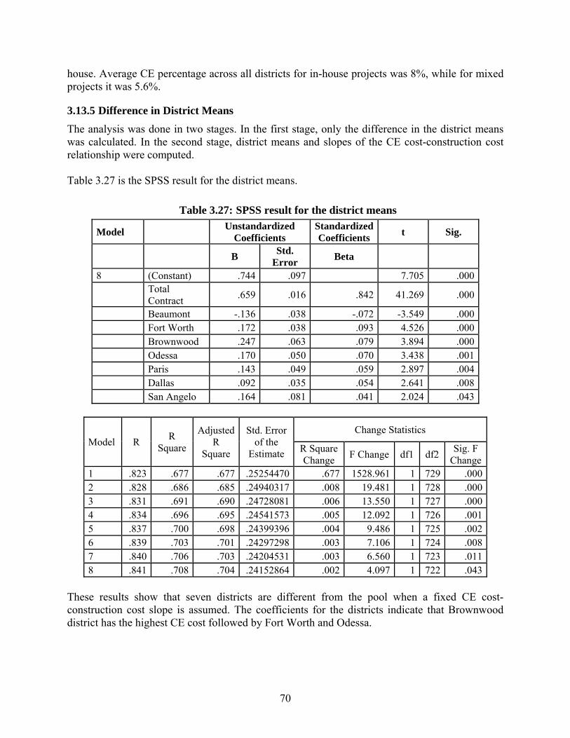
70

house. Average CE percentage across all districts for in-house projects was 8%, while for mixed projects it was 5.6%.

3.13.5 Difference in District Means The analysis was done in two stages. In the first stage, only the difference in the district means was calculated. In the second stage, district means and slopes of the CE cost-construction cost relationship were computed. Table 3.27 is the SPSS result for the district means.

Table 3.27: SPSS result for the district means



B Std. Error Beta

8 (Constant) .744 .097 7.705 .000

Total Contract .659 .016 .842 41.269 .000

Beaumont -.136 .038 -.072 -3.549 .000 Fort Worth .172 .038 .093 4.526 .000 Brownwood .247 .063 .079 3.894 .000 Odessa .170 .050 .070 3.438 .001 Paris .143 .049 .059 2.897 .004 Dallas .092 .035 .054 2.641 .008 San Angelo .164 .081 .041 2.024 .043

Model R R Square

Adjusted R

Square

Std. Error of the

Estimate

Change Statistics

R Square Change F Change df1 df2 Sig. F

Change1 .823 .677 .677 .25254470 .677 1528.961 1 729 .0002 .828 .686 .685 .24940317 .008 19.481 1 728 .0003 .831 .691 .690 .24728081 .006 13.550 1 727 .0004 .834 .696 .695 .24541573 .005 12.092 1 726 .0015 .837 .700 .698 .24399396 .004 9.486 1 725 .0026 .839 .703 .701 .24297298 .003 7.106 1 724 .0087 .840 .706 .703 .24204531 .003 6.560 1 723 .0118 .841 .708 .704 .24152864 .002 4.097 1 722 .043

These results show that seven districts are different from the pool when a fixed CE cost-construction cost slope is assumed. The coefficients for the districts indicate that Brownwood district has the highest CE cost followed by Fort Worth and Odessa.

71

Figures 3.26, 3.27, and 3.28 show fitted lines for CE cost for various districts.

Figure 3.26: Estimation of District CE Costs based on 731 TxDOT Projects: Log-Log Plot

Figure 3.27: Estimation of District CE Costs based on 731 TxDOT Projects: Normal Plot

72

Figure 3.28: Estimation of District CE Costs based on 731 TxDOT Projects: Zoomed Plot

Beaumont district has a lower CE percentage than average while all other significantly different districts have higher CE percentage. Brownwood has the highest CE percentage. Fort Worth, Odessa, Paris, and San Angelo have very close CE percentages. Figures 3.29 and 3.30 show the pattern of CE percentage for different contract amounts.

73

Figure 3.29: Estimation of Percentage District CE Costs based on 731 TxDOT Projects:

Normal Plot

Figure 3.30: Estimation of Percentage District CE Costs based on 731 TxDOT Projects:

Zoomed Plot

74

The charts show that CE percentage is high for small contract amount and it decreases as the contract amount increases. This district result is similar to the project type analysis. Brownwood has the highest CE percentage while Beaumont has the lowest. According to the project type analysis, TS and BR projects have the highest CE percentage but the Brownwood district did not do those types of projects in significant number (only 1 BR project). There is no clear explanation for Brownwood’s high CE percentage.

3.13.6 Difference by CE Provider Consultant involvement can affect CE percentage of any district. To find this, interaction of total contract amount with the provider as a switch variable was submitted. Total construction engineering cost was selected as a dependent variable while In-house, districts, and interaction of In-house and districts were selected as switch variables. Total contract amount and interaction of In-house and contract amount were selected as independent variables. Stepwise regression was run to see how preliminary engineering cost is affected after considering interaction of districts with total contract amount and CE provider. The SPSS result of this analysis is shown in Table 3.28.

Table 3.28: SPSS analysis results



B Std. Error Beta 10 (Constant) .827 .099 8.380 .000 Total Contract .650 .016 .832 40.762 .000 Beaumont -.139 .038 -.074 -3.670 .000 Fort Worth .178 .037 .096 4.751 .000 Brownwood .261 .063 .083 4.164 .000 In*Odessa .210 .051 .084 4.155 .000 In*Paris .182 .050 .074 3.648 .000 IH*CONTRACT -.012 .003 -.077 -3.647 .000 Dallas .111 .035 .065 3.187 .001 In*San Angelo .274 .091 .060 3.002 .003 In*Abilene*Cont .024 .009 .053 2.603 .009

Model R R Square

Adjusted R

Square

Std. Error of the

EstimateChange Statistics

R Square Change


Change10 .846 .716 .712 .23854392 .003 6.775 1 720 .009

In the table, the e‘In’ and ‘IH’ prefixes imply In-house projects for that district (different intercept) and the ‘Cont’ suffix implies interaction with total contract amount (different slopes).

75

In the coefficient table, the In-house variable (binary variable for In-house project) is not significant, however, interaction of In-house project with total contract amount (IH*Contract) is significant. Because it has a negative coefficient, In-house projects are found to have less CE percentage than mixed projects. However, for 4 districts—namely, Odessa, Paris, San Angelo, and Abilene—In-house projects have a higher CE percentage than average. In-house projects in the San Angelo district have the highest coefficient, followed by the Brownwood district, while Beaumont has the lowest. Figures 3.31, 3.32, and 3.33 are the graphical representations of the results.

Figure 3.31: Estimation of District CE Costs with consultant involvement: Log-Log Plot

76

Figure 3.32: Estimation of District CE Costs with consultant involvement: Normal Plot

Figure 3.33: Estimation of District CE Costs with consultant involvement: Zoomed Plot

The above charts show that the Brownwood district has the highest CE percentage even though its coefficient is lower than that of In-house San Angelo. This is because total contract amount

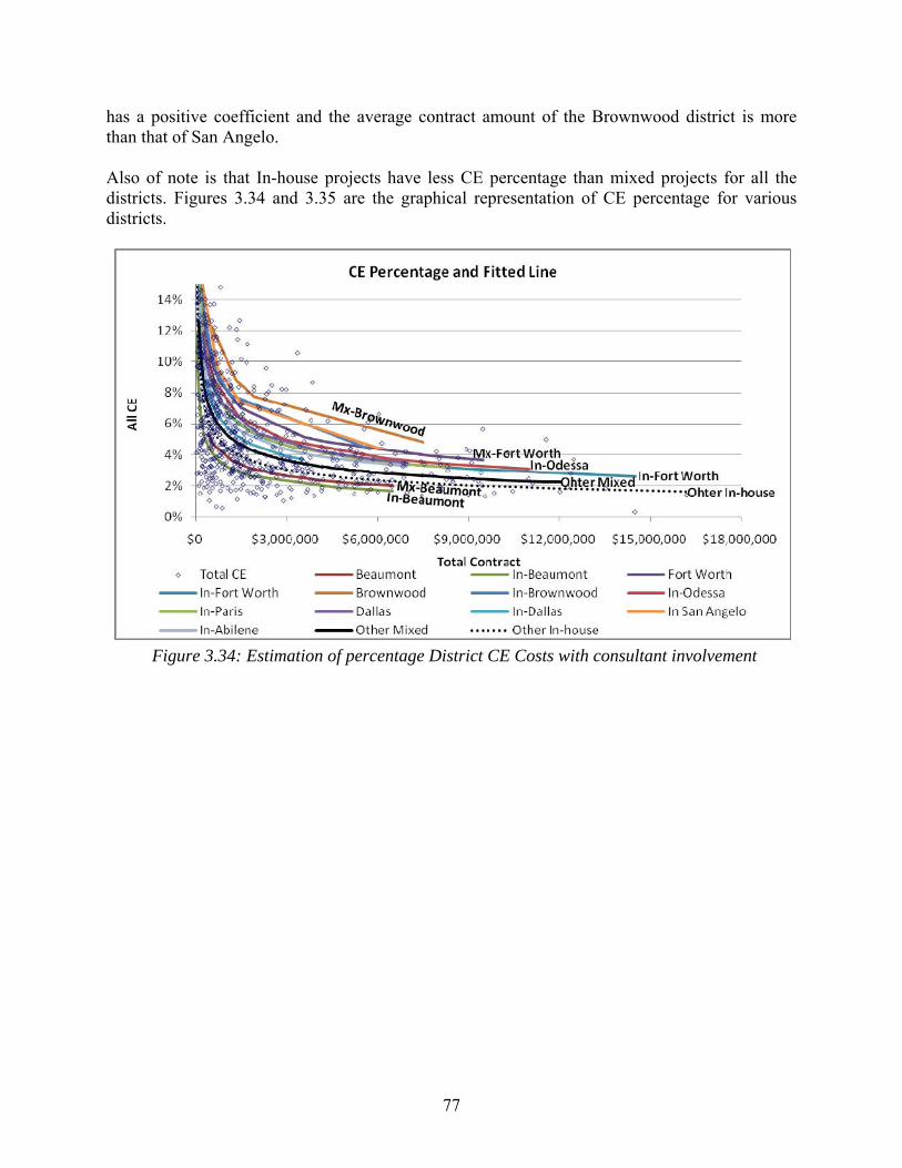
77

has a positive coefficient and the average contract amount of the Brownwood district is more than that of San Angelo. Also of note is that In-house projects have less CE percentage than mixed projects for all the districts. Figures 3.34 and 3.35 are the graphical representation of CE percentage for various districts.

Figure 3.34: Estimation of percentage District CE Costs with consultant involvement

78

Figure 3.35: Estimation of percentage District CE Costs with consultant involvement:

Zoomed Plot

The charts show that CE percentage decreases with increase in contract amount. In-house and Mixed projects both decrease at about the same rate. Similar to previous results, In-house projects exhibit slightly less CE percentage than mixed ones. This analysis shows that In-house projects have less construction engineering cost than mixed projects, for a given district and contract amount.

3.13.7 Section Conclusion This section presented the results of a statistical analysis of PE and CE costs for TxDOT projects let for construction in FY06 and 07. The time span of the data was limited in order to reduce the effect of inflation. Data on 1832 construction projects was obtained from the Construction Division and the Finance Division of TxDOT. Of these 1832 projects, CE charges on 731 completed projects were analyzed separately.

Stepwise regression analysis was performed in the SPSS statistical analysis program. The independent variables introduced were project construction cost, project type (binary variable), and PE provider (binary variable: Fully In-house or Mixed), as well as interaction terms for Project Type─Construction Cost and Provider Type─Construction Cost.

The CE cost analysis found that project construction cost and project type account for about 72% of the variance in CE costs. For all project types the percentage CE decreases as project cost increases. In terms of relative CE cost, the project types were found to rank as follows, from most to least costly: Traffic Signals, Bridge Replacement, Landscape, Other, Overlays, and Sealcoats.

79

In district level analysis it was found that In-house projects are significantly different from Mixed projects in CE cost. In-house projects have lower CE percentage than Mixed projects for any district and contract amount. There were some anomalies in the results. For example, average percentage CE of In-house was 8% while for Mixed, it was 5.6% but regression analysis at 95% confidence showed that district–wise, In-house CE percentage is less; while for project types, it is not significantly different.

It must be stressed that the CE results are based only on those project let and completed in FY 06-07. Naturally, those are smaller and simpler projects. There was insufficient data on larger and more complex project types to determine if they are statistically more or less expensive in CE.

3.14 Conclusions This report presented the results of a statistical analysis of PE and CE costs for TxDOT projects let for construction in FY06 and 07. The time span of the data was limited in order to reduce the effect of inflation. Four issues are addressed in this analysis:

1. The cost of engineering for projects done with in-house staff compared to using consultant forces.

2. The differences in engineering costs for different project types and across a range of work scopes.

3. The quality of engineering for projects done with in-house staff compared to using consultant forces.

4. The differences in engineering costs across TxDOT districts. Data on 1832 construction projects was obtained from the Construction Division and the Finance Division of TxDOT. Of these 1832 projects, PE charges on 1371 projects in construction or completed were selected for analysis, and CE charges on 731 completed projects were analyzed separately. There were 26 different project types. Each project type’s preliminary engineering data is available at the function code level. However, even though there are many projects done entirely with in-house staff, no projects done entirely by consultants were found, so PE provider was designated as Fully In-house or Mixed. Stepwise regression analysis was performed in the SPSS statistical analysis program. The independent variables introduced were project construction cost, project type (switch variable), PE provider (binary variable: Fully In-house or Mixed), District (switch variable for 25 TxDOT districts), as well as interaction terms for Project Type─Construction Cost and Provider Type─Construction Cost.

3.14.1 PE Costs The PE cost analysis found that project construction cost, PE provider, and project type account for about 75% of the variance in PE costs. For all project types the percentage PE decreases as project cost increases, confirming economies of scale. If a letting program includes multiple small-dollar projects, it will have a higher PE cost than one with large projects. Viewed another

80

way, PE output (dollars let per dollar PE cost) must vary depending on size and complexity of the projects being designed. The analysis found that there are statistically significant differences in PE costs between Fully In-house projects and Mixed projects. For all project types, the statistically estimated PE percentage for Fully In-house projects is lower than for Mixed projects. These results were presented in graphs. In gross terms, PE percentages for In-house and Mixed projects are 1.29% and 6.20% respectively for the full set of projects studied. However, in most cases the construction cost of the median In-house project is smaller than that of the median Mixed project. If construction cost is a proxy for project scope, then Fully In-house projects are smaller in scope than Mixed projects. To test a direct comparison between in-house and consultant costs, the data was analyzed at the function code level. The ten most used functions, which make up to 88% of the total preliminary engineering cost, were analyzed. It was found that, by one methodology, consultant PE costs were 5.2 times as high as in-house PE charges.

3.14.2 Differences in Project Types, Districts, and PE Quality In terms of relative costliness, the project types were found to rank in the following order from most to least costly: Widen Freeway (including New Location Freeway and Convert Non-Freeway to Freeway), Upgrade Freeway to Standards, Interchange, Bridge Replacement, Bridge Widen/Rehab, Widen Non-Freeway, Miscellaneous Construction, Other, Landscape, Overlays and Sealcoats. When PE costs across TxDOT districts were compared, it was found that PE provider (In-house or Mixed) is still the largest factor in PE cost differences. The next most important factor is project size as measured by construction cost. After these two are taken into account, differences among project types emerge. But ultimately it was found that Mixed projects in Laredo, El Paso, San Antonio had higher PE percentage than average while Childress, Yoakum, and Amarillo had lower. It is speculated that the high cost districts may have higher involvement of historically underutilized businesses, but that data was not available for this analysis. To compare the quality of PE on Mixed projects to In-house projects, the absolute value of change orders on each project was analyzed. No significant difference in change order rates for In-house and Mixed projects was found.

3.14.3 CE Costs

The CE cost analysis found that project construction cost and project type account for about 72% of the variance in CE costs. For all project types the percentage CE decreases as project cost increases. In terms of relative CE cost, the project types were found to rank as follows, from most to least costly: Traffic Signals, Bridge Widening and Rehabilitation, Bridge Replacement, Landscape, Other, Overlays, and Sealcoats. Similar to PE analyses, district level analysis was conducted for CE charges. It was found there was significant difference between in-house and mixed projects. Average In-house projects exhibit less CE percentage than average Mixed projects. However, In-house projects of San

81

Angelo, Odessa, and Fort Worth showed more CE percentage than Mixed projects in those districts respectively. Percentage CE in all the districts and for all the project types decreases with an increase in contract amount, ranging from 2% to 23 % of the total contract amount but more than 90% projects had CE percentage less than 15%. CE results are based only on those projects let and completed in FY 06-07. Naturally, those are smaller and simpler projects. There was insufficient data on larger and more complex project types to determine if they are statistically more or less expensive in CE.

3.14.4 Recommendations Project type and size are not the only measures of PE needs; two projects of the same type and equal construction cost may have entirely different PE requirements. The fact that a project required consultant PE suggests that the in-house staff, for whatever reason, could not do the work. Moreover, more complex project types are rarely done In-house. Thus, the portfolio of Mixed projects is different from Fully In-house in scope and complexity. In that case, a gross PE percentage for each class is a simplistic and misleading measure, and caution should be exercised in interpreting such numbers from any DOT. Even when project type, size and PE provider are taken into account, El Paso, Laredo, and San Antonio districts were found to have higher than typical PE costs for Mixed projects. It is not clear why this is the case, and further research is recommended to clarify whether this was a one-time phenomenon for the specific data studied, or whether there are unique conditions contributing to higher costs in these districts. Throughout the analyses, the differences found in costs between in-house and mixed projects were consistent and large, so much so as to raise speculation for the reasons. While this statistical analysis cannot uncover the reasons, it does bring into question the accuracy of the in-house charges. A further line of inquiry would be to compare the total PE charges in each district to the number of full-time staff working on PE, to determine how much of their time is actually charged to projects.

83

Chapter 4. Optimization of Emergency Response among TxDOT Maintenance Sections

4.1 Introduction Task 3: Optimization of Emergency Response among TxDOT Maintenance Sections The objective of this task was to develop a methodology for determining district maintenance personnel needs and locations.

4.2 Work Order Statement for Task 3 The following is the work order that was provided by TxDOT for this task: Project Title: Optimization of Emergency Response among TxDOT Maintenance Sections. Project Scope: It is Department policy to ensure that department personnel (not contractors) be the first responders to road-related emergencies, especially in the rural areas. Given future expected budget constraints, a methodology is needed to determine personnel needs and their location given:

• Historical emergency demands

• Maintenance office overhead costs

• Crew travel costs

• Efficiency maximum and minimum office sizes The analytical approach will be to examine the tradeoff between interoffice travel costs and office overhead costs. With many offices, overhead is high but travel is low; with few offices, overhead is low but travel costs are high. Linear programming is the tool of choice for this kind of optimization in the sense of minimizing the total of travel plus office costs while meeting needed (estimated) emergency level of service. Linear programming is a high-efficiency way of determining the optimum among large numbers of alternatives. This tool can also be used for “what-if” analyses such as changing population patterns, increased emergency demands, increased travel costs, increased office costs, and alternative new section locations. The scope of this project is to construct a pilot model for the San Antonio district to determine its feasibility and usability. TxDOT will supply available data or best estimates to the principal researchers. They will then produce the equation structure for the model and use a commercial optimization application to run it. The researchers will also perform sensitivity analyses to determine the impact of the critical parameters. The Department will then assess the results of the pilot study to determine whether this would be useful statewide for personnel planning.

4.3 Results The following is the final technical memorandum that was submitted for this task on December 2, 2009.

84

Maintenance Section Location Optimization Model Authors: Dr. Leon Lasdon and Dr. John Butler

Project Director: Ron Hagquist TxDOT Strategic Policy and Performance Management Office Operations Research Coordinator Researchers: Dr. Leon Lasdon The David Bruton Jr. Chair in Business Support Systems McCombs School of Business University of Texas at Austin Dr. John Butler Academic Director, Energy Management & Innovation Center Clinical Associate Professor of Finance McCombs School of Business University of Texas at Austin

4.3.1 Purpose of the Model This is an Excel-based location optimization model that can be used to examine the economics of maintenance section locations within TxDOT districts. It analyzes the tradeoffs among section office overhead, lease or sale value, and cost of travel to work locations. It can be used to see if any existing sections could be candidates for closing or consolidation, and to optimize the placement of possible new sections in an expanding urban area. Closing a section office eliminates overhead cost and gains the Department the lease income or sale value; however, a closed section must have its maintenance duties provided by other sections, increasing travel cost and losing productivity due to the increased travel time. For example, with many offices, overhead cost is high but travel is low; with few offices, overhead is low but travel is high. This model uses a high-efficiency optimization algorithm called linear programming to simultaneously determine the minimum-cost number and location of a given set of existing sections. However, it can also determine the optimum given a proposed set of new sections, such as might occur in a growing metro district. Note: This model does not deal with the issue of emergency response. This was covered in a study, "Optimization of Emergency Response Among TxDOT Maintenance Sections," submitted to the Maintenance Strategic Plan workgroup chaired by Walter McCullough, dated 5/27/2009.

4.3.2 How the Model Works

The model makes an economic evaluation of a series of cases: one section, two sections, three sections, etc. For each of these cases it determines the optimum (i.e., the least-cost) configuration of that number of sections. So for example, for the two-section case, the model determines which

85

two of the number of existing sections would produce the lowest total cost—total cost being defined as the sum of travel costs, overhead costs, and property sale value. The model uses a "math engine" called linear programming, which is an optimization algorithm that efficiently determines the minimum cost without doing trial-and-error computations of all possible combinations. This is accomplished by converting all relevant data into simultaneous equations and inequalities, which the linear programming algorithm solves and within which it finds the optimum solution. This process also has the benefit of being mathematically assured the optimum is reached, even though all combinations were not explicitly evaluated. Further explanation of linear programming can be found in any management science or operations research textbook. Linear programming is useful for many such optimization problems because the number of combinations can be too large to manage by simple trial-and-error. For example, all possible permutations for a 6-section case would require 1,237 individual computations; the number of computations go up rapidly with the number of sections considered since the formula for permutations for n different things arranged in groups of r objects is given by: nPr = n!/(n-r)!, and this must be computed and summed for each of n-1 cases. This model automatically invokes the built-in “solver” in Excel with which to accomplish the linear programming aspect of the computations.

4.3.3 How the Model Is To Be Used This model contains an example analysis of the Houston district to provide guidance for data entry. (Note: these Houston numbers were just rough approximations to attempt to be realistic but are not precise enough to provide meaningful results for that district.) Note: This model can evaluate a maximum of 13 sections due to Excel limitations. Data is input by editing these sample data in the yellow fields. The following steps are also explained as text in the Excel model:

1. Go to the Input Data sheet and click on "Edit Demand for Trips, Overhead, and Distance Data."

2. Change economic data if desired.

3. Type in the names of the sections to be evaluated; check the boxes next to these.

4. Enter the data on annual trip demand, office overhead, and likely property sale value.

5. Click on "Done With Data Edits." This opens the Distance Data worksheet.

6. Edit the names of the sections and fill in the travel distances between them. Click on "Done With Data Edits."

7. Click on "Edit Travel Cost Data." Click on "Done With Travel Cost Data."

8. Decide on whether you want to include lost wage (productivity) during travel to cover work from a closed section. Click on appropriate button.

86

4.3.4 Outputs The primary results of the model are displayed in Figure 4.1, showing the total costs (less revenues from sale or lease of closed sections) with the optimal (least cost) configurations of case runs of the various numbers of open sections.

Figure 4.1: Example of chart showing total costs with optimum configurations

In this illustrative chart, the optimal number of sections would be 8 selected out of the existing 11, with the configuration detail for that shown elsewhere in the output. Figure 4.2 illustrates the location model while Figure 4.3 provides the initial worksheet for selecting model options.

Figure 4.2: Location model

87

Figure 4.3: Initial worksheet for selecting stages of the model, data entry or running options

Clicking on the first blue rectangle in Figure 4.3 takes the user to the first data input screen. When this is completed, the user is brought back to this screen to select (if desired) the second blue rectangle. When all data is entered, the user is finally brought back to this screen to select the desired assumption about lost productivity during travel to cover the work needs of a closed section from another section. Clicking the first rectangle takes the user to the initial data entry screen, shown in Figure 4.4. The yellow fields are the parameters that can be changed, and example data are shown as a guide.

Figure 4.4: Initial data entry screen

88

Up to 13 sections can be evaluated by this model. In the example shown in Figure 4.4, 11 sections are being analyzed as shown by the checked boxes.

Discount and growth rates To make an apples-to-apples comparison between the overhead costs associated with keeping a facility open and the revenue from the sale of a property, some adjustments are required. Clearly, the sale of a property is a one-time inflow to TxDOT and should reflect the "total" value of the property. In finance this is often referred to as the future value discounted to a present value. However, the annual overhead fees would continue to occur for as long as the facility is open. To correct this we chose to convert the one-time sales values to "annualized" sales. If the property was sold for $S dollars today, we can solve for the value $X such that receiving $S today is equivalent to receiving $X per year forever. If we assume that the value of $X would grow at g% year, the Gordon Growth Model implies $S = $X(1+g)/(r-g). Since we observe $S we can solve for the annualized sales value $X as X = S(r-g)/(1+g) where r is TxDOT's cost of capital. For TxDOT a good first estimate of r would be the rate at which TxDOT could borrow money to fund projects and an estimate of g could be inflation. We use these annualized sales values in the objective function. Note also that the “demand” is from historical data on work crew trips per year. “Overhead” is the fixed operating cost for the section building. A closed section could be leased or sold; the estimated sale option value is used in this model. Figure 4.5 provides an example of distance data entry. The distances are road-travel distances to allow computation of travel time between sections. When these data are filled in, the user clicks on the blue “Done with Data Edits” box, which returns them to the first screen.

89

Figure 4.5: Distance data entry

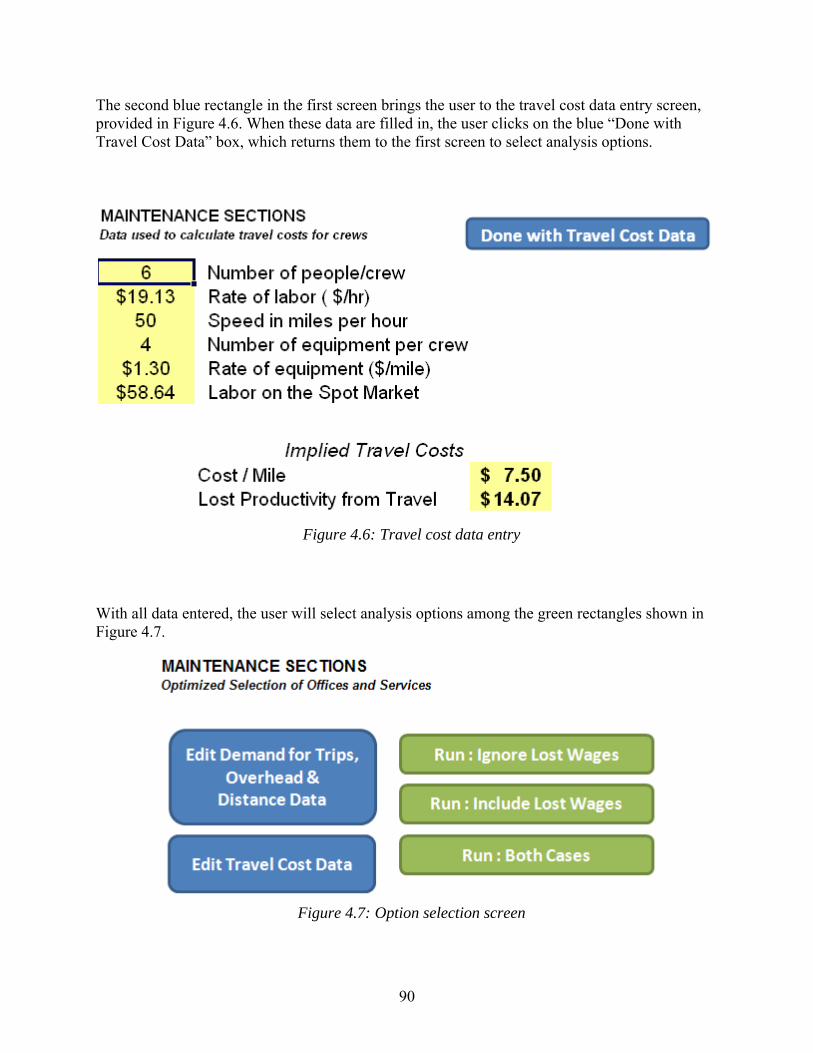
90

The second blue rectangle in the first screen brings the user to the travel cost data entry screen, provided in Figure 4.6. When these data are filled in, the user clicks on the blue “Done with Travel Cost Data” box, which returns them to the first screen to select analysis options.

Figure 4.6: Travel cost data entry

With all data entered, the user will select analysis options among the green rectangles shown in Figure 4.7.

Figure 4.7: Option selection screen

91

If an existing section were closed, then its work would be handled from another nearby section, which would entail additional travel from there. A major issue in the analysis is whether to include the lost productivity during the travel, expressed as wages lost to the department; the green rectangles give the user the option to choose. Clicking on one begins the computations and brings up the output screens, shown in Figure 4.8.

Figure 4.8: Output: “Summary” of results worksheet

These results are explained in the following pages. Figure 4.9 provides an example of an output sheet detail.

Figure 4.9: Detail of output sheet

In this case, both options of including and excluding lost wages were analyzed. The charts show the costs of operating various numbers of sections. The first chart shows that if lost productivity is considered, then keeping 8 of the 11 sections is the least-cost configuration. In the second case, which ignores lost productivity from travel, no savings are obtained from closing any sections, so the lowest cost is from keeping all 11 sections open. Figure 4.10 shows which sections are kept open under the optimal least-cost configuration for both wage cases. Open sections are shown as 1’s, and closed sections shown as 0’s.

92

Figure 4.10: Open and closed sections

93

Figure 4.11 shows summaries of the travel and overhead costs and property sale values for the two cases.

Figure 4.11: Cost information

Figures 4.12 and 4.13 provide the data summary screen and a detail of the summary screen. Please note the following regarding the data in Figures 4.12 and 4.13:

• If a district only serves itself, it is listed without detail, e.g., Brazoria.

• If a district serves another district, the total travel miles are listed after it in parentheses. For example, Central Houston crews travel a total of 24 miles, including 8-mile trips to West Harris and 16-mile trips to North Harris.

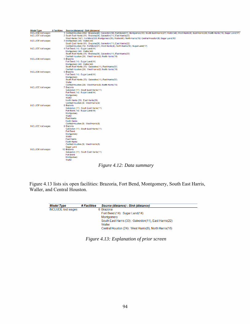
94

Figure 4.12: Data summary

Figure 4.13 lists six open facilities: Brazoria, Fort Bend, Montgomery, South East Harris, Waller, and Central Houston.

Figure 4.13: Explanation of prior screen

95

Chapter 5. The Needs and Funding Options for Texas Mega-Bridge Replacement Projects

5.1 Introduction Task 4: The Needs and Funding Options for Texas Mega-Bridge Replacement Projects The objective of this task was to develop a report on what projects are defined as “mega-bridge” projects, basic information on the need for each project, project costs, and a proposed plan to provide for the funding of these projects outside of the normal HBP process.

5.2 Work Order Statement for Task 4 The following is the work order that was provided by TxDOT for this task:

Texas has the largest number of highway bridges in the nation. As of September 2008, there were 50,572 bridges in the state, and of that total, 10,878 (21.5%), were considered structurally deficient, functionally obsolete or sub-standard for load capacity. As pointed out in the recent “2030 Committee: Texas Transportation Needs Report,” the predicted total cost to place these deficient bridges could be in the range of $34 billion through the year 2030. The primary means that TxDOT has used in the past to fund the replacement of deficient bridges is through the Federal Highway Bridge Program (HBP). A current estimate of the funding available under this program is approximately $250 Million per year for the next 10 years. As can be seen by this disparity between anticipated needs and available funding, the HBP is thoroughly inadequate to handle the magnitude of needed bridge replacement projects. Making this situation worse is the anticipated requirement to carry out several “mega-bridge” projects (defined as on-system projects costing $100 Million or more and off-system projects costing $20 Million or more) over the near to mid-term (next 15 years). In order to provide the legislature and the general public with the basic facts relating to this funding gap and its consequences, a report will be developed that provides a background to the problem, what projects are defined as “mega-bridge” projects, basic information on the need for each project, project costs, and a proposed plan to provide for the funding of these projects outside of the normal HBP process. The material included in the report should be detailed enough to provide adequate justification for each project without causing undue concern over the bridges current conditions. The report should calculate an annual level of investment that would be required to replace all of the “mega-bridges” over the next 15 years. TxDOT’s Bridge Division will provide a listing of the projects to be included in the report, current construction cost estimates, inspection reports and environmental reports (if available). Bridge Division personnel will be available to discuss issues and answer questions as needed.

5.3 Results Following is the technical memorandum that was submitted by CTR for this task.

96

Mega-Bridges in Texas Author: Rob Harrison

5.4 Background Texas Bridges and the Role of Mega-bridges

5.4.1 Texas’ Extensive Bridge Network Texas has the largest system of state highway bridges in the United States. In 2007, while Texas ranked first in both number of bridges (more than 50,000) and deck area (more than 417 million square feet), it was only third in annual federal funding for bridges, receiving $362 million. Bridges require scheduled maintenance and inspection to ensure they can continue to safely carry increasing traffic volumes and higher numbers of loaded trucks. All state bridges are regularly inspected to ensure that they meet the original design load when constructed and remain safe for travelers. In Texas, the results of these inspections are recorded as part of the Bridge Inspection and Appraisal Program (BRINSAP), which is the main source for state and federal bridge analyses, the latter leading to federal funding allocations.

5.4.2 How Many Bridges Are in Texas? BRINSAP records bridge data on both the TxDOT system (termed “on system”), which is supported by partial allocations of federal funds, and the city and county system (termed “off-system”), which is supported by state and county/city funding. In 2007 there were 33,500 on-system bridges, which carried 584 million vehicles per day, and 17,567 off-system bridges, which carried 57 million vehicles per day. TxDOT is responsible for the inspection of on- and off-system bridges, as well as the maintenance, rehabilitation, and replacement of all on-system bridges. TxDOT also shares in the costs for rehabilitation and replacement of off-system bridges, with the remainder funded by cities and counties, which also perform the required maintenance of off-system bridges. Federal funds pay for a substantial portion of the rehabilitation and replacement costs of both on- and off-system bridges. Bridges are typically designed with an average life expectancy of 50 years. In Texas, new bridge construction was heavy during the late 1950s through the 1960s when the state built much of its interstate highway system. Therefore, many of these bridges will be due for replacement between 2009 and 2030. In addition, many rural bridges on the off-system were built in the period 1930-1955 to lower design standards because truck weights were significantly less than current limits. Accordingly, increasing numbers of such bridges are being identified for replacement or posted at lower truck weights because of inadequate funding for their replacement.

5.4.3 2030 Committee In May 2008, the Texas Transportation Commission appointed a volunteer committee of respected business leaders designated as the 2030 Committee. The charge was to provide an independent, yet authoritative, assessment of the Texas transportation infrastructure and mobility

97

needs from 2009 to 2030. The Committee directed a team of state university researchers, who utilized TxDOT pavement and bridge data to determine the state highway assets, and data from TxDOT and the state metropolitan planning organizations (MPOs) to derive the mobility needs over the 22-year period of 2009 to 2030. Details of the methods used are found in the full Committee Report drafted at the end of December 2008 and approved by the Commission in late February 2009, after a period of public review and comment. The 2030 bridge needs are summarized in Box 1.

The total investment is expressed in 2008 dollars—which does not allow for any future inflation. The figures include the full delivery cost of each bridge replacement, capturing the complete range of engineering activities necessary to replace a bridge and tie it into the highway system. The federal portion of a qualified on-system bridge replacement, though substantial, follows a strict formula defining the extent of the bridge structure that excludes a number of the necessary engineering activities. This places a financial burden on TxDOT and other entities to provide the remaining funds. The portion of the $36 billion investment that comprised mega-bridges1 was estimated at $6.1 billion for the 22-year period or $278 million per year, a figure approaching the total federal allocation for all Texas bridge categories in 2007. This technical note does not attempt to predict future mega-bridge needs because a number of key assumptions have to be made about mobility needs and traffic growth. It describes the current number and estimated cost of those that have been identified by the Bridge Division as candidates for financial assistance. The next section presents this in greater detail.

5.5 Texas Mega-Bridges in 2009 Mega-bridges are special structures with a number of unusual characteristics and can therefore be categorized in a number of ways. Clearly, physical size is a key attribute, as is the reason for a bridge’s location, such as crossing a wide expanse of water. A bridge can also be characterized by its importance to the regional highway system it serves—for example, how far the user is

1 In the 2030 Committee Report such bridges are termed “Special and Large.”

Box 1: 2030 Committee Bridge Recommendations

• Replace on-system structurally deficient and substandard load-only bridges by 2012.

• Replace remaining structurally deficient, substandard load-only and functionally obsolete bridges by 2030.

• Increase inspection and maintenance activities to maintain safety and extend life.

• Investment needed: $36 billion total; $1.6 billion per year.

98

diverted if the bridge is closed and how much time that takes—and the role it plays in benefiting users and the regional economy where it is located. This technical note defines mega-bridges by the estimated cost of their replacement because its main focus is to provide an estimate of current needs for this category of bridges. Bridges, of course, can be kept in service for very long periods just like other large capital-intensive civil engineering projects such as dams, sea walls, and canal systems. The economic truth is that this strategy of perpetual operation is inefficient because the owner—in this case, TxDOT—faces substantial and recurring maintenance and rehabilitation costs, on an annual basis, to keep the structure at an acceptable level of integrity and service. Finally, if the community wishes to keep the bridge in service for cultural reasons—as is the case in Europe—alternative structures are built to carry the increased traffic volumes. The precise time when it is economically efficient to replace a structure rather than continue to fund replacement activities can be calculated and is part of normal life cycle models. The mega-bridges reported in 2009 are those that have exceeded their economic life and need replacement. The financial needs used in this note as trigger points for full replacement are $100 million for the on-system and $25 million (at $ 2009 costs) for the off-system. It should also be noted that federal funds allocated to TxDOT through the Highway Bridge Program can only, at best, provide a portion of the total investment needed to replace mega-bridges. As with many large capital projects, the funds come from a variety of sources2. It is also indicative of why a number of mega-bridges have a toll charge to help meet bonding repayment and maintenance needs. The categories of mega-bridge designs most commonly undertaken by TxDOT are described by a combination of ownership (on- and off-system) and location in the next section, together with an example of a project in each category to describe typical characteristics in greater detail.

5.6 Mega-Bridge Categories

5.6.1 Major Navigable Waterway Crossings Major navigable waterway crossings generally require large vertical clearances above the water and long span lengths to clear navigation channels. In addition, because crossings of major waterways may be few and far between, many of these types of facilities carry multiple lanes of traffic in each direction. The high cost for this type of structure results from long approach lengths due to the required high vertical clearance, long main span lengths to prevent piers from encroaching on the shipping channels, wide decks to support multiple lanes of traffic, and difficult construction conditions over water. These factors make them some of the highest cost structures TxDOT constructs. The Harbor Bridge in Corpus Christi is an example of this type of structure (shown in Figure 5.1). The existing bridge was built in 1959 and consists of 5 truss spans, 15 welded plate girder spans, and 37 prestressed concrete girder spans. The total bridge length measures 5,819 feet and

2 More details are given in the Frequently Asked Questions section of this note.

99

the structure carries the six-lane divided US 181 highway over the Corpus Christi Ship Channel. Traffic counts indicate that approximately 50,000 vehicles use this facility daily.

Figure 5.1: Corpus Christi Harbor Bridge

Due to the steel construction of the existing Harbor Bridge and the highly corrosive saltwater environment it inhabits, the structure requires continuous cleaning, painting, and maintenance. More than $15 million has been spent on maintaining the Harbor Bridge in the past 15 years. An additional $15 million in such maintenance work is scheduled over the next year. The age of the bridge means that such costs will no doubt accelerate in the future. The Harbor Bridge’s physical dimensions currently restrict the Port of Corpus Christi from serving larger ships. The bridge’s clearance restricts and limits the size of vessels that can enter and exit the Channel. In order to eliminate recurring high maintenance costs, remove the vertical and horizontal clearance restrictions on the Ship Channel, and improve the capacity of US 181, TxDOT plans to replace the current Harbor Bridge with a new, higher bridge. This new structure will also have a longer span and will be designed to be less vulnerable to saltwater corrosion. Preliminary plan work on this new bridge has begun. It is estimated that construction costs of the replacement structure and associated roadwork and interchanges will be in excess of $700 million.

5.6.2 Major Thoroughfares Major thoroughfares are generally associated with the National Highway System. These facilities were initiated in the 1950s and have become entrenched as the foundation of our transportation system. As capacity demands have required the expansion of these highways, high population and commercial densities have entrapped the roadway, reducing options or pushing the expansion upward rather than outward. There are many examples of entrapped facilities throughout the state. The combination of restricted space, complicated geometry, expensive real

100

estate, and large numbers of vehicles using the facility make the replacement of such a structure very complicated and very expensive. In addition, traffic control is particularly difficult and expensive on these types of projects. The elevated portion of IH 345 in Dallas is an excellent example of a very high volume structure in an urban setting. This facility is actually a group of over twelve interconnected bridges that must be considered as a whole when discussing replacement. Traffic counts indicate that between 150,000 and 200,000 vehicles use this facility every day. Main lane structures within one mile north and south of the IH 30 intersection (pictured in Figures 5.2 and 5.3) are elevated and supported primarily by a steel superstructure. Maintenance projects are keeping the bridge in service, but at a significant cost. It is estimated that replacement costs of just the four main structures will be in excess of $350 million. Figure 5.2 is a view of the intersection of IH 30 (lower level, only partially visible), IH 345 (upper level), and the two direct connectors in between.

Figure 5.2: Intersection of IH 30

101

Figure 5.3: Ongoing inspection and maintenance of the structure

5.6.3 Complex Highway Interchange A complex highway interchange is comprised of a grade separation(s) and ramps that allow traffic on two intersecting highways to pass through the juncture without interrupting traffic flow. The interchange at US 290/IH 610 in Houston is an example of a complex urban structure. Due to its proximity to IH 10, the US 290/IH 610 interchange allows traffic to flow to multiple economic centers within the city. Houston is the fourth largest metropolitan area in the United States and is continually growing. Northwest Houston has one of the largest growth rates in this area with US 290 as its only major route. Based on the most recent national study conducted by the Texas Transportation Institute, Houston congestion has deteriorated to over 56 hours of annual delay, wasting over 42 gallons of fuel, and costing approximately $18.80 per hour per traveler. This interchange alone sees over 250,000 vehicles per day with each vehicle navigating through complicated traffic patterns (Figure 5.4). This results in unacceptable operational levels, particularly during peak times. The facility does not have adequate capacity for the amounts of traffic it currently supports and it will be wholly unable to meet future demands.

102

Figure 5.4: A view of the US 290/IH 610 interchange in Houston

A proposed project for this location calls for the replacement of existing structures in addition to adding over 3,000,000 square feet of new bridge structures.

5.6.4 Major Off-System Bridge Structures Bridges located on city streets or county roads and owned by local governmental agencies (e.g., City; County; Water District) are identified as off-system. (Bridges on state-owned highways are identified as on-system.) The majority of these bridges are relatively smaller, normally ranging from 20-ft to 400-ft in length. There are, however, a few off-system structures that exceed these limits and range from 1,000-ft to 4,000-ft in length. These bridges are identified as major off-system bridges. An example of a major off-system bridge is the Herbert E. Schmidt Causeway which is now described. The Herbert E. Schmidt Causeway, also known as the Seawolf Parkway at Pelican Island Channel, was constructed in 1960. This bridge is owned and operated by the Galveston County Navigational District No. 1. The 3,239-ft long structure consists of a single leaf bascule steel deck truss main span, 9-plate girder major approach spans, and 42 prestressed concrete minor approach spans. The bascule concrete piers sit on concrete footings supported by timber piles and are protected by a timber fender system. Fender systems provide protection for piers from impacts caused by marine vessels. The approach spans are supported on concrete pile trestle bents. In 1995, TxDOT entered into a construction contract in the amount of $2.9 million for the rehabilitation of the structure. The project consisted of replacing the timber fender system, installing sheet piling to protect the interior bents from scour (the erosion of the soil from beneath the footings), and making repairs to the concrete spans, the truss members of the bascule span, and the railing. In addition several maintenance contracts have been completed and funded entirely by the Galveston County Navigational District No. 1 and have totaled nearly $1 million.

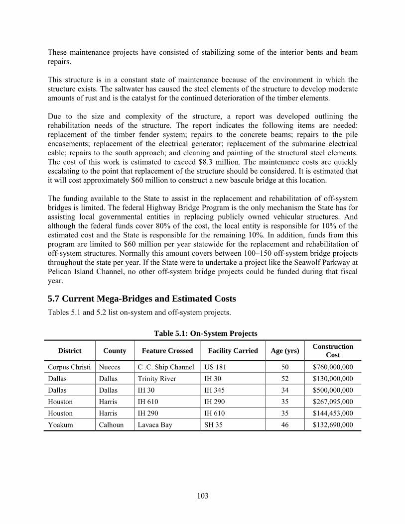
103

These maintenance projects have consisted of stabilizing some of the interior bents and beam repairs. This structure is in a constant state of maintenance because of the environment in which the structure exists. The saltwater has caused the steel elements of the structure to develop moderate amounts of rust and is the catalyst for the continued deterioration of the timber elements. Due to the size and complexity of the structure, a report was developed outlining the rehabilitation needs of the structure. The report indicates the following items are needed: replacement of the timber fender system; repairs to the concrete beams; repairs to the pile encasements; replacement of the electrical generator; replacement of the submarine electrical cable; repairs to the south approach; and cleaning and painting of the structural steel elements. The cost of this work is estimated to exceed $8.3 million. The maintenance costs are quickly escalating to the point that replacement of the structure should be considered. It is estimated that it will cost approximately $60 million to construct a new bascule bridge at this location. The funding available to the State to assist in the replacement and rehabilitation of off-system bridges is limited. The federal Highway Bridge Program is the only mechanism the State has for assisting local governmental entities in replacing publicly owned vehicular structures. And although the federal funds cover 80% of the cost, the local entity is responsible for 10% of the estimated cost and the State is responsible for the remaining 10%. In addition, funds from this program are limited to $60 million per year statewide for the replacement and rehabilitation of off-system structures. Normally this amount covers between 100–150 off-system bridge projects throughout the state per year. If the State were to undertake a project like the Seawolf Parkway at Pelican Island Channel, no other off-system bridge projects could be funded during that fiscal year.

5.7 Current Mega-Bridges and Estimated Costs Tables 5.1 and 5.2 list on-system and off-system projects.

Table 5.1: On-System Projects District County Feature Crossed Facility Carried Age (yrs) Construction

Cost

Corpus Christi Nueces C .C. Ship Channel US 181 50 $760,000,000Dallas Dallas Trinity River IH 30 52 $130,000,000Dallas Dallas IH 30 IH 345 34 $500,000,000Houston Harris IH 610 IH 290 35 $267,095,000Houston Harris IH 290 IH 610 35 $144,453,000Yoakum Calhoun Lavaca Bay SH 35 46 $132,690,000

104

Table 5.2: Off-System Projects

District County Feature Crossed Facility Carried Age (yrs) Construction Cost

Dallas Dallas Trinity River Sylvan Ave 51 $45,959,355Fort Worth Tarrant Trinity River W. 7th 96 $25,959,000

Houston Galveston Pelican Island Channel Seawolf Pkwy 49 $60,000,000

5.8 Mega-bridges: Frequently Asked Questions Are there mega-bridges that may need to be replaced that are not currently in TxDOT’s database of projects for construction? At this time there are only two such projects: the replacement of the IH 345 bridges in Dallas and the replacement of the Herbert E. Schmidt Causeway (Seawolf Parkway at Pelican Island Channel) in Galveston County, as discussed in this report. However, as demand continues to increase and the highway infrastructure ages, mega-bridges will be needed. For example, new mobility investments will require expensive multi-level interchanges. As a result, identifying and securing the funding for these projects will become increasingly challenging. Why is planning these projects necessary now? The citizens of Texas expect a safe, efficient, functional facility that is convenient and economical. The structures identified in this memo need substantial rehabilitation or replacement (M&R) expenditures. Due to the high cost of M&R, together with the critical nature of these facilities to the traveling public, planning must be initiated to ensure the funds are available when the structures are replaced. Can the public expect work to begin on these projects during the next 10-15 years? Most of these bridges carry high traffic volumes with a high percentage of truck traffic. Some are also nearing the end of their economic life cycle. As a result, they have an accelerated rate of M&R costs and have been identified as priority projects within the next 15 years. Are there environmental or other constraints that would affect when or even if these projects are constructed? Environmental constraints are always present and must always be considered. In many cases, mega-bridges are sited in new, complementary locations that must meet all federal and state environmental legislation. However, for these projects it is likely that environmental concerns would impact their location rather than precluding their replacement. The high usage of these facilities is evidence of our need for them. The momentum of the project generated by high demand will bolster our efforts to identify and implement innovative solutions to environmental issues. (Let’s discuss this.) Are there funding sources already secured for any of these projects, and if so, what type of funding sources (both TxDOT and Non-TxDOT) are currently used or anticipated? Many of these projects already have funding sources associated with them. The primary sources include the following TxDOT categories: Category 6—Structures Replacement and Rehabilitation, Category 2—Metropolitan Area Corridor Projects, Category 10—Supplemental Transportation Projects, Category 7—Metropolitan Mobility and Rehabilitation, Category 5—

105

Congestion Mitigation and Air Quality Improvement. Also, several projects, especially the off-system projects for which the only TxDOT funding mechanism allowed is Category 6, have local government funding components. The high cost of mega-bridges makes it unlikely that traditional funding sources, especially the Federal Highway Program and its Highway Trust Fund, will be able to meet all costs. New and nontraditional sources such as state bonds (generated from gas tax revenue or general revenue), tolling, public-private partnerships, and various local funding sources will be necessary to bridge the funding gap for many of these projects. Partnering in this way also brings forward the date when the work can begin and the economic benefits enjoyed. Does TxDOT need to develop a special funding category to handle these projects? Each of these mega projects is unique and a single new category would not appreciably aid in the development of these projects. One policy would be to develop these projects under the appropriate existing category, and spread the funding over many different funding sources to match both the need and particular circumstances of the project. Should TxDOT bank funds over several years to handle the expense of these projects when they come up? While Highway Bridge Program (HBP) replacement projects are typically fully funded in the year they are scheduled for construction, it may be beneficial to spread the cost of mega-bridge projects over multi-years to avoid disrupting the overall program in any one year. (Note: discuss the use of term HEP) Should these projects be subject to a selection rating process? There are insufficient funds to address all bridge needs simultaneously, so projects must be ranked. Mega-bridge projects typically should be subject to cost-benefit (C/B) analysis, making it possible to compare potential projects and allocate their position in a multi-year program. Should such a selection process be based on a strict cost/benefit analysis, on the bridge’s condition, or should it be first-come, first-served? The selection process should be based on a comprehensive C/B approach that includes vehicle operating costs, time savings, the cost of alternative actions like rehabilitation, and the strategic role the structure plays in the highway system. What are the best estimates for costs for proposed work, taking into consideration construction dates and factoring in construction and materials cost inflation? Estimating inflation is not necessary and can lead to substantial bias if the estimated rate is incorrect—which is almost always the case. It is best to estimate the costs for all candidates using the best, most recent, actual costs and then expressing the estimate in costs for that year—FY 2008 costs, for example. Those wishing to estimate future needs can then use a variety of inflation rates to predict multi-year program costs. In any future year, for example 2012, the FY 2008 costs can be accurately updated by the actual inflation rates that were experienced.

107

Chapter 6. Tracking the U.S. Fiscal Stimulus Investments in Texas

6.1 Introduction Task 5: Tracking the U.S. Fiscal Stimulus Investments in Texas Transportation Projects Supervised by TxDOT and Developing New Economic Impact Models for Project Selection The objective of this task was to track the development of TxDOT stimulus inputs to FHWA and build a relational database.

6.2 Work Order Statement for Task 5 The following is the work order that was provided by TxDOT for this task: Task description is based on a meeting with Senior TxDOT Managers on March 16, 2009 and subsequent meetings with CST staff members responsible for collecting ARRA data for construction projects and potential CTR and LBJ School researchers staffing the work. The American Recovery and Reinvestment Act (ARRA) of 2009—more commonly referred to as the “Fiscal Stimulus” investment program—allocates $ 27.5 billion to U.S. State Departments of Transportation and Federal Land Agencies for highway infrastructure. ARRA Funds require an increased level of data reporting to insure that they meet the stated objectives of the legislation. The Federal Highway Administration (FHWA) in concert with the Office of the Secretary of Transportation (OST) and the other modes within the Department of Transportation (DOT) are currently determining the type and detail of data to be provided on each project. CST is responsible for much of the AARA funding but other Divisions such as design, aviation, and public transportation will also have to report economic impact data to FHWA. The first drafts of ARRA reporting documentation required data on the direct employment (jobs) and payroll (financing) associated with prime contractors and all sub-contractors to be provided on a four week cycle. This will be collected and then submitted by each state DOT to FHWA who will then integrate it with other data bases like the Financial Management Information Systems (FIMS) and report the impacts to Congress and the general public, the latter via a web site. TxDOT is taking this as an opportunity to strengthen its understanding of the economic impacts of highway investments, and enhance the models used to select projects for the established investment programs. This work is part of a multi-year effort. In Year One (FY 09), a CTR team led by Robert Harrison worked closely with Construction Division staff to track the development of TxDOT stimulus inputs to FHWA and build a relational data base to allow estimation of a wider range of economic impacts for Texas. The results are intended to be used by TxDOT staff to estimate calibrated indirect and induced impacts of Texas highway investment, in addition to the direct impacts, so allowing the potential incorporation of a wide range of benefits into the current project selection process.

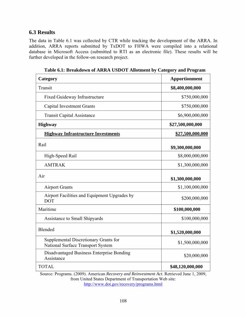
108

6.3 Results The data in Table 6.1 was collected by CTR while tracking the development of the ARRA. In addition, ARRA reports submitted by TxDOT to FHWA were compiled into a relational database in Microsoft Access (submitted to RTI as an electronic file). These results will be further developed in the follow-on research project.

Table 6.1: Breakdown of ARRA USDOT Allotment by Category and Program

Source: Programs. (2009). American Recovery and Reinvestment Act. Retrieved June 1, 2009, from United States Department of Transportation Web site:

http://www.dot.gov/recovery/programs.html

Category Apportionment

Transit $8,400,000,000

Fixed Guideway Infrastructure $750,000,000

Capital Investment Grants $750,000,000

Transit Capital Assistance $6,900,000,000

Highway $27,500,000,000

Highway Infrastructure Investments $27,500,000,000

Rail $9,300,000,000

High-Speed Rail $8,000,000,000

AMTRAK $1,300,000,000

Air $1,300,000,000

Airport Grants $1,100,000,000

Airport Facilities and Equipment Upgrades by DOT $200,000,000

Maritime $100,000,000

Assistance to Small Shipyards $100,000,000

Blended $1,520,000,000

Supplemental Discretionary Grants for National Surface Transport System $1,500,000,000

Disadvantaged Business Enterprise Bonding Assistance $20,000,000

TOTAL $48,120,000,000

109

6.3.2 TxDOT Plan for ARRA Funds

• Total Funding to Texas highway program: $2.25 billion

o Available for direct use by Texas Transportation Commission: $1.7 billion

$500 million for maintenance projects

• 266 roadway and bridge maintenance/rehabilitation projects

o 182 roadway maintenance projects ($370 million)

o 27 roadway rehabilitation projects ($73 million)

o 47 bridge projects ($31 million)

o 10 local/regional safety enhancement projects ($30 million)

o Total: $505,675,806

$1.2 billion for significant projects

• 29 projects across state ranging from toll roads to rail to freeway maintenance

o $500 million for metropolitan planning organizations

• 10 aviation projects ($49.7 million)

• 39 public transportation projects ($32.8 million)

• April 30th: 200 construction maintenance projects approved by TxDOT and Texas Transportation Commission

o $274 million of ARRA funds

o Approximately 2,655 jobs will be supported

Sources TxDOT puts stimulus funds to work. (2009, February 26). Texas Department of Transportation.

Retrieved June 3, 2009, from http://www.txdot.gov/news/007-2009.htm TxDOT puts stimulus funds to work: construction, maintenance projects will start this spring. (2009,

March 5). Texas Department of Transportation. Retrieved June 3, 2009, from http://www.txdot.gov/news/009-2009.htm

Commission approved stimulus projects. (2009, March 5). Texas Department of Transportation. Retrieved June 3, 2009, from ftp://ftp.dot.state.tx.us/pub/txdot-info/stimulus/project_list_030509.pdf

TxDOT approves first group of stimulus project contracts. (2009, April 30). Texas Department of

Transportation. Retrieved June 9, 2009, from http://www.dot.state.tx.us/news/019-2009.htm

6.3.3 ARRA Job Creation Outlook

• “$789 billion will create or save 3.5 million jobs over the next two years”

• Jobs in industries such as clean energy, healthcare; over 90% of jobs in private sector

• Estimated Effect

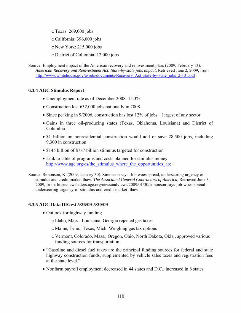
110

o Texas: 269,000 jobs

o California: 396,000 jobs

o New York: 215,000 jobs

o District of Columbia: 12,000 jobs Source: Employment impact of the American recovery and reinvestment plan. (2009, February 13).

American Recovery and Reinvestment Act: State-by-state jobs impact. Retrieved June 2, 2009, from http://www.whitehouse.gov/assets/documents/Recovery_Act_state-by-state_jobs_2-131.pdf

6.3.4 AGC Stimulus Report

• Unemployment rate as of December 2008: 15.3%

• Construction lost 632,000 jobs nationally in 2008

• Since peaking in 9/2006, construction has lost 12% of jobs—largest of any sector

• Gains in three oil-producing states (Texas, Oklahoma, Louisiana) and District of Columbia

• $1 billion on nonresidential construction would add or save 28,500 jobs, including 9,300 in construction

• $145 billion of $787 billion stimulus targeted for construction

• Link to table of programs and costs planned for stimulus money: http://www.agc.org/cs/the_stimulus_where_the_opportunities_are

Source: Simonson, K. (2009, January 30). Simonson says: Job woes spread, underscoring urgency of

stimulus and credit market thaw. The Associated General Contractors of America, Retrieved June 3, 2009, from: http://newsletters.agc.org/newsandviews/2009/01/30/simonson-says-job-woes-spread-underscoring-urgency-of-stimulus-and-credit-market- thaw

6.3.5 AGC Data DIGest 5/26/09-5/30/09

• Outlook for highway funding

o Idaho, Mass., Louisiana, Georgia rejected gas taxes

o Maine, Tenn., Texas, Mich. Weighing gas tax options

o Vermont, Colorado, Mass., Oregon, Ohio, North Dakota, Okla., approved various funding sources for transportation

• “Gasoline and diesel fuel taxes are the principal funding sources for federal and state highway construction funds, supplemented by vehicle sales taxes and registration fees at the state level.”

• Nonfarm payroll employment decreased in 44 states and D.C., increased in 6 states

111

• Construction employment decreased in 41 states, increased in 6 states, and remained unchanged in 3 states and D.C.

Source: Simonson, K. (Ed.). (2009, May 29). The Data DIGest, 9(18).

6.3.6 AGC Data DIGest 6/8/09-6/12/09

• Stimulus plan has already funded 1% of $275 billion for construction work

o $1.5 billion for state highways

o Small federal reimbursements for construction work

o An allowance for work that has not yet been reimbursed

• Construction activity has slowed due to economic conditions; there is hope that stimulus will help improve situation

• Cost of steel, fuel have increased

• Pay for full-time construction workers was 1% higher than that for the average full-time worker in private industry

Source: Simonson, K. (Ed.). (2009, June 12). The Data DIGest, 9(20).

6.3.7 Input-Output Models

• RIMS II

o I-O Table

Distribution of inputs purchased and outputs sold

RIMS Multipliers

For any region consisting of one or more counties

For any industries in national I-O table

490 industries, 38 industry aggregations

o Accuracy

Within 10% of more expensive methods

o Data

Industry category

Year of expenditure

Location

o Results

Earnings

Output

112

Jobs

• IMPLAN

o Multipliers

Type I multipliers

Type III multipliers

Generated for employment, output, value added, personal income, total income

o BEA data

o Builds data from top to bottom (from national to state to county level)

Source: Lynch, T. (2000, October). Analyzing the economic impact of transportation projects using RIMS II, IMPLAN and REMI. Retrieved June 2, 2009, from Florida State University, Institute for Science and Public Affairs Web site: http://www.cefa.fsu.edu/econimpact.pdf

6.3.8 A Stimulating Time for Construction?

• Economic Influences

o Continuing decline in bank lending

o Rising unemployment

o Lack of consumer interest

o ARRA

• Construction-Related Stimulus Spending

o Transportation ($49 billion)

o Buildings ($35 billion)

o Energy/technology ($30 billion)

o Water/environment ($21 billion)

• Conditions Tied to Stimulus Money

o Davis-Bacon: workers must be paid in accordance with local median wage

o Buy American: favors American producers over foreign producers

o More stringent reports on jobs, payroll, etc.

• Construction Spending

o Declined in private residential, public, and private nonresidential

o Materials

Increases in the industrial and institutional sectors

Decreases in the developer-financed sector

o Outlook for 2009

113

Residential: -2% to +2%

Nonresidential: -3% to -9%

Total: -1% to -7%

o Change in PPI and CPI since 2003

PPI: +31%

CPI: +16%

o PPI for various products

Decreases in most categories from year-ago values, such as highway & street construction and No. 2 diesel fuel

Increases from year-ago values in asphalt paving mixtures & blocks, concrete products, and gypsum products

o Materials in 2009 will be less expensive than in 2008 but are expected to increase beyond that

o Housing Outlook

Decreases in construction spending, building permits, and housing starts

Single-Family spending totals should begin improvement in late 2009

Multi-family totals will likely not improve until 2011

• Construction Employment (12-month changes)

o Residential jobs: -3%

o Nonresidential jobs: -10%

o Architecture/Engineering: -7%

o All states experienced a decline or no change in construction employment except ND and LA (more jobs due to Hurricane Katrina recovery process)

• Summary

o Nonresidential spending expected to decline over the next two years

o Residential spending may decline a bit in 2009, but is expected to improve in 2010

o Total construction spending expected to begin increasing in 2010

o Materials costs will decline this year, but should increase in 2010

o Labor costs are expected to increase slowly over the next two years Source: Simonson, K. (2009, July 9). A stimulating time for construction? Forum presented at the

meeting of the Austin Chapter Associated General Contractors, Austin City Council Chamber.

115

Appendix A: Regression Results of Function Code PE Cost Analysis

Function 102 Model Summary

Model R

R Square

Adjusted R Square



F Change df1 df2

Sig. F Change

1 .517 .268 .259 .71900595

0 .268 31.800 1 87 .000

Coefficients


Standardized Coefficients

t Sig. B Std. Error Beta1 (Constant) 3.870 .192 20.141 .000

In-house -1.180 .209 -.517 -5.639 .000


Model R

R Square

Adjusted R Square



F Change df1 df2

Sig. F Change

1 .457a .209 .207 .80765490

0 .209 90.316 1 342 .000

2 .493b .243 .238 .79134983

6 .034 15.238 1 341 .000

Coefficients




In-house -1.057 .111 -.457 -9.503 .000 2 (Constant) 1.908 .540 3.537 .000

In-house -1.062 .109 -.459 -9.744 .000 Total (Contract) .334 .085 .184 3.904 .000

116


Model R

R Square

Adjusted R Square



F Change df1 df2

Sig. F Change

1 .272 .074 .071 .644834142404533 .074 27.417 1 344 .000

2 .302 .091 .086 .639783970330176 .017 6.452 1 343 .012

Coefficients




Total Contract .344 .066 .272 5.236 .000 2 (Constant) 1.756 .435 4.040 .000

Total Contract .350 .065 .276 5.365 .000 In-house -.498 .196 -.131 -2.540 .012


Model R

R Square

Adjusted R Square



F Change df1 df2

Sig. F Change

1 .517a .268 .266 .755368435

6 .268 121.761 1 333 .000

2 .535b .286 .282 .747067292

4 .018 8.441 1 332 .004

117

Coefficients



t Sig.B Std. Error Beta1 (Constant) 3.704 .063 58.426 .000

In-house -.922 .084 -.517 -11.035 .0002 (Constant) 2.231 .511 4.366 .000

In-house -.937 .083 -.526 -11.317 .000Total Contract (Log) .237 .082 .135 2.905 .004


Model R

R Square

Adjusted R Square



F Change df1 df2

Sig. F Change

1 .584 .341 .340 .6978603617 .341 228.008 1 440 .000

2 .614 .377 .374 .6797354127 .035 24.778 1 439 .000

Coefficients




In-house -1.027 .068 -.584 -15.100 .0002 (Constant) 2.536 .369 6.867 .000

In-house -1.025 .066 -.583 -15.466 .000Total Contract (Log) .292 .059 .188 4.978 .000

118


Model R R Square

Adjusted R Square



F Change df1 df2

Sig. F Change

1 .360 .130 .128 .798278848

4 .130 93.615 1 629 .000

2 .475 .226 .224 .753367843

9 .096 78.229 1 628 .000

Coefficients



t Sig.B Std. Error Beta1 (Constant) .389 .374 1.041 .298

Total Contract (Log) .576 .060 .360 9.675 .0002 (Constant) .933 .358 2.604 .009

Total Contract (Log) .573 .056 .358 10.201 .000In-house -.660 .075 -.311 -8.845 .000


Model R R Square

Adjusted R Square



F Change df1 df2

Sig. F Change

1 .494 .244 .242 .6942011992 .244 145.955 1 452 .000

2 .632 .399 .396 .6196981073 .155 116.216 1 451 .000

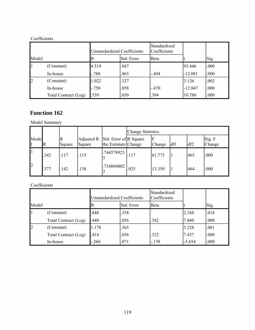
119

Coefficients





In-house -.750 .058 -.470 -12.847 .000Total Contract (Log) .539 .050 .394 10.780 .000


Model R

R Square

Adjusted R Square



F Change df1 df2

Sig. F Change

1 .342 .117 .115 .744578923

5 .117 61.773 1 465 .000

2 .377 .142 .138 .734884002

2 .025 13.350 1 464 .000

Coefficients




Total Contract (Log) .440 .056 .342 7.860 .0002 (Constant) 1.178 .365 3.228 .001


120


Model R R Square

Adjusted R Square



F Change df1 df2

Sig. F Change

1 .419 .175 .174 .714769871

4 .175 118.501 1 558 .000

2 .469 .220 .218 .695515544

9 .045 32.322 1 557 .000

Coefficients




Total Contract (Log) .565 .052 .419 10.886 .0002 (Constant) 1.018 .322 3.159 .002



Model R R Square

Adjusted R Square



F Change df1 df2

Sig. F Change

1 .306 .093 .089 .916318803

3 .093 21.032 1 204 .000

2 .394 .156 .147 .8865606290 .062 14.925 1 203 .000

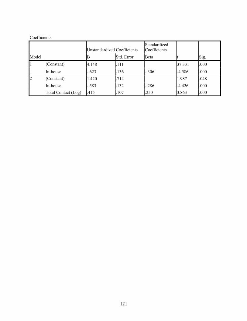
121

Coefficients





In-house -.583 .132 -.286 -4.426 .000Total Contact (Log) .415 .107 .250 3.863 .000

Special Studies for TxDOT Administration in FY...

Documents

Transcript of Special Studies for TxDOT Administration in FY...