D I S S E R T A T I O N

Special sets of real numbers

and variants of the Borel Conjecture

ausgefuhrt zum Zwecke der Erlangung des akademischen Gradeseines Doktors der technischen Wissenschaften

unter der Leitung von

Ao.Univ.Prof. Dipl.-Ing. Dr.techn. Martin GoldsternInstitut fur Diskrete Mathematik und Geometrie

E104

eingereicht an der Technischen Universitat WienFakultat fur Mathematik und Geoinformation

von

Wolfgang Wohofskye0025959

wolfgang.wohofsky@gmx.at

http://www.wohofsky.eu/math/

Ottakringer Straße 215/4/3/11, 1160 Wien

Wien, am 19. September 2013

Kurzfassung

In meiner Dissertation beschaftige ich mich mit einem Teilgebiet der Men-genlehre: ich untersuche Fragen uber “spezielle” Teilmengen der reellenZahlen, die durch Konzepte aus der Analysis, Maßtheorie und Topologiemotiviert sind. Ihre Losung erfordert oft mengentheoretische Methoden wiezum Beispiel die sogenannte “Erzwingungsmethode” (engl.: “forcing”), dadie meisten dieser Fragen nicht durch die gewohnlichen Axiome der Mengen-lehre (ZFC) “entscheidbar” sind.

Insbesondere untersuche ich “kleine” (oder: “spezielle”) Mengen, typischer-weise Elemente gewisser Sigma-Ideale auf den reellen Zahlen, wie beispiels-weise die aus der Maßtheorie stammenden Lebesgueschen Nullmengen, oderdie noch viel kleineren “starken Nullmengen” (engl.: “strong measure zerosets”).

ZFC erlaubt keine Folgerungen der Art “alle Mengen von kleiner/großer Kar-dinalitat liegen innerhalb/außerhalb eines gegebenen Ideals”. Zum Beispielkann die sogenannte “Borel-Vermutung” (engl.: “Borel Conjecture”; be-nannt nach Emile Borel; es ist die Aussage, daß alle starken Nullmengenhochstens abzahlbar sind) aus den ZFC-Axiomen weder bewiesen noch wider-legt werden.

Galvin, Mycielski und Solovay bewiesen einen auf diesem Gebiet zentralenSatz, indem sie eine Verbindung (mittels Translationen) zwischen starkenNullmengen und sogenannten (aus der Topologie stammenden) mageren Men-gen zeigten. Dieser Satz ermoglicht es, den zum Begriff der starken Null-menge “dualen” Begriff der “stark mageren Menge” (engl.: “strongly meagerset”) – und damit auch die “duale Borel-Vermutung” (engl.: “dual BorelConjecture”) – einzufuhren.

In Kapitel 1 wird eine kurze Ubersicht uber alle fur die Dissertation re-levanten Konzepte gegeben.

Kapitel 2 ist eine gemeinsame Arbeit mit meinem DissertationsbetreuerMartin Goldstern, Jakob Kellner und Saharon Shelah: wir zeigen, daß es ein

2

Modell von ZFC gibt, in dem sowohl die Borel-Vermutung als auch die dualeBorel-Vermutung gilt (mit anderen Worten: in dem es weder uberabzahlbarestarke Nullmengen noch uberabzahlbare stark magere Mengen gibt).

In Kapitel 3 wird eine Verstarkung dieses Resultats gezeigt, in dem derBegriff der stark mageren Mengen durch den (schwacheren) Begriff der “sehrmageren Mengen” (engl.: “very meager sets”) ersetzt wird.

In Kapitel 4 wird gezeigt, daß sowohl die Borel-Vermutung als auchdie duale Borel-Vermutung mit einer definierbaren Wohlordnung der reellenZahlen vertraglich ist.

In Kapitel 5 wende ich mich wieder dem oben erwahnten Satz von Galvin-Mycielski-Solovay zu und zeige, daß man ihn auf verschiedene allgemeinereStrukturen ausdehnen kann.

In Kapitel 6 definiere ich eine neue Klasse von “kleinen Mengen” (unddie zugehorige Variante der Borel-Vermutung) und entwickle Methoden zurUntersuchung derselben (unter Annahme der Kontinuumshypothese).

In Kapitel 7 beschreibe ich kurz, auf welche Weise die Konzepte ausKapitel 6 weiter verallgemeinert werden konnen.

3

Acknowledgment

Above all, I wish to thank my advisor Martin Goldstern for his supportand numerous helpful and enjoyable conversations: his guidance, patience,knowledge about many areas of set theory (and other mathematics), and hissuperior teaching skills were invaluable for my studies and my work.

I thank Saharon Shelah and Jakob Kellner for many helpful and inspiringconversations, in particular in the context of our joint paper BC+dBC. I amalso grateful to the anonymous referee of this paper.

Furthermore, I thank Sy D. Friedman, the head of the Kurt Godel ResearchCenter; the KGRC is such a great place to meet colleagues, give seminartalks, and attend great lectures and research talks.

I gratefully acknowledge the following (partial) support: DOC fellowship ofthe Austrian Academy of Sciences (OAW); US National Science FoundationGrant No. 0600940; Austrian Science Fund (FWF): P21651-N13 and P23875-N13 and EU FP7 Marie Curie grant PERG02-GA-2207-224747; FWF grantP21968.

Many thanks to Tomek Bartoszynski, Jorg Brendle, Stefan Geschke, MarcinKysiak, Adrian Mathias, Heike Mildenberger, Janusz Pawlikowski, DilipRaghavan, Marcin Sabok, Stevo Todorcevic, Tomasz Weiss, Piotr Zakrzewski,Jindrich Zapletal, and other set theorists I talked with at various places, forinspiring and helpful conversations.

I also thank Piotr Borodulin-Nadzieja for inviting me to Wroc law, and PhilippSchlicht for inviting me to Bonn, and for being generous hosts during my stay.

I am happy about many great conversations and the nice time I spent withmy fellow students Carolin Antos-Kuby, Arthur Fischer, Ajdin Halilovic,Stefan Hoffelner, Peter Holy, Giorgio Laguzzi, Anda-Ramona Tanasie, andFabio Tonti, as well as with many other colleagues, such as Dana Bartosova,Andrew Brooke-Taylor, David Chodounsky, Vera Fischer, Jana Flaskova,

4

Radek Honzık, Yurii Khomskii, Vadim Kulikov, David Schrittesser, Kather-ine Thompson, Jonathan Verner, Zoltan Vidnyanszky, and Lyubomyr Zdom-skyy.

Especially, I am happy about the nice time I spent with Thilo Weinert: wehad many interesting and fruitful discussions about various topics (of settheory and beyond).

Moreover, I wish to mention Thomas Johnstone: I am glad that I can lookback at our time together in Vienna, especially our very long conversationsabout set theory.

I thank my fellow students of my undergraduate studies, especially, I thank“den Sechzehn” – my close colleagues during that time – for being goodfriends and for helping each other, as well as Angelika Standteiner for beinga close friend during my beginning studies of set theory.

I deeply thank all my friends and relatives for their support: especially, mybest friend Sigrid Prandler for her encouragement over the years, and myparents for their caring, encouragement, and unconditional love.

5

Preface

In my thesis, I investigate questions about subsets of the real line. Whilethese questions are motivated by concepts from analysis, measure theory,and topology, their resolution often needs set-theoretic methods – such asthe method of forcing –, as these questions (the prototypical such question isHilbert’s first problem about the continuum hypothesis) may be not resolv-able by ZFC (the usual axioms of set theory).

In particular, I investigate small (special) sets, i.e., elements of certain naturalσ-ideals on the real numbers (or collections only closed under taking subsets),such as the measure zero sets and the much smaller strong measure zero sets.

ZFC typically does not allow conclusions of the form “all sets of small/largecardinality are inside/outside of a certain collection”. For instance, theBorel Conjecture – the statement that all strong measure zero sets are atmost countable – can neither be proved nor refuted from the ZFC axioms.

Annotated contents

Chapter 1 Introduction

I give some historical background and review several concepts and re-sults that are relevant to my thesis, such as the notion of strong measurezero, the Galvin-Mycielski-Solovay characterization of strong measurezero sets via translations of meager sets, the notion of strongly mea-ger, Borel Conjecture, dual Borel Conjecture, etc.; furthermore, I givea very informal overview of my joint paper [GKSW] (i.e., Chapter 2).

Chapter 2 Borel Conjecture and dual Borel Conjecture

This chapter contains my joint paper with Martin Goldstern, JakobKellner, and Saharon Shelah: We show that it is consistent that theBorel Conjecture and the dual Borel Conjecture hold simultaneously.

6

Chapter 3 A strengthening of the dual Borel Conjecture

We show that a strengthening of the dual Borel Conjecture holds in ourmodel of BC+dBC: there are no uncountable very meager sets there(the very meager sets always form a σ-ideal containing all stronglymeager sets). This is joint work with Saharon Shelah.

Chapter 4 A projective well-order of the reals and BC/dBC

Using methods from [FF10], we show how to modify Laver’s proof ofCon(BC) to get a model of “BC + there exists a projective well-orderof the reals”. Similarly, we show the analogous result for dBC, usingmethods from [FFZ11]. This is joint work with Sy D. Friedman.

Chapter 5 Galvin-Mycielski-Solovay theorem revisited

I give versions of the Galvin-Mycielski-Solovay theorem for more gen-eral settings: I provide a version for the generalized Cantor space 2κ forweakly compact κ, as well as a version for separable locally compactgroups. On the other hand, I show that the Galvin-Mycielski-Solovaycharacterization consistently fails for the Baer-Specker group Zω.

Chapter 6 Sacks dense ideals and Marczewski Borel Conjecture

Let MBC (Marczewski Borel Conjecture) be the assertion that there areno uncountable s0-shiftable sets (those sets that can be translated awayfrom each set in the Marczewski ideal s0). So MBC is the analogue toBC (dBC) with meager (measure zero) replaced by s0. To investigatewhether MBC is consistent, I introduce the notion of “Sacks dense ide-als” to explore the family of s0-shiftable sets. Even though Con(MBC)remains unsettled, I present several results about Sacks dense ideals.

Chapter 7 P dense ideals for tree forcing notions

In Chapter 6, problems regarding the Marczewski ideal s0 are consid-ered, which is connected to Sacks forcing S. In this chapter, I brieflydiscuss whether Sacks forcing can be replaced by other tree forcing no-tions (such as Silver forcing, Laver forcing, etc.) in the arguments ofChapter 6.

7

Contents

Kurzfassung 2

Acknowledgment 4

Preface 6

1 Introduction 101.1 Historical background . . . . . . . . . . . . . . . . . . . . . . . 101.2 Preliminaries . . . . . . . . . . . . . . . . . . . . . . . . . . . 111.3 An overview of the proof of Con(BC+dBC) . . . . . . . . . . 24

2 Borel Conjecture and dual Borel Conjecture 32Introduction . . . . . . . . . . . . . . . . . . . . . . . . . . . . 32

2.1 Ultralaver forcing . . . . . . . . . . . . . . . . . . . . . . . . . 382.2 Janus forcing . . . . . . . . . . . . . . . . . . . . . . . . . . . 572.3 Almost finite and almost countable support iterations . . . . . 682.4 The forcing construction . . . . . . . . . . . . . . . . . . . . . 912.5 The proof of BC+dBC . . . . . . . . . . . . . . . . . . . . . . 1062.6 A word on variants of the definitions . . . . . . . . . . . . . . 113

3 A strengthening of the dual Borel Conjecture 1163.1 Janus forcing kills very meager sets . . . . . . . . . . . . . . . 1173.2 Strengthening of dBC in the final model . . . . . . . . . . . . 119

4 A projective well-order of the reals and BC/dBC 1224.1 A projective well-order and BC . . . . . . . . . . . . . . . . . 1234.2 A projective well-order and dBC . . . . . . . . . . . . . . . . . 126

5 Galvin-Mycielski-Solovay theorem revisited 1305.1 GMS for 2κ (κ ≥ ℵ0 weakly compact) . . . . . . . . . . . . . . 1305.2 GMS for separable locally compact groups . . . . . . . . . . . 1425.3 Failure of GMS for Zω . . . . . . . . . . . . . . . . . . . . . . 160

8

6 Sacks dense ideals and Marczewski Borel Conjecture 1686.1 The Marczewski ideal s0 and the MBC . . . . . . . . . . . . . 1696.2 Sacks dense ideals . . . . . . . . . . . . . . . . . . . . . . . . . 1726.3 Confining s∗0 by Sacks dense ideals (Jf )f∈ωω . . . . . . . . . . 1776.4 Confining s∗0 even more: the Vitali Sacks dense ideal E0 . . . . 1856.5 Intersecting σ-ideals dense in Sacks forcing . . . . . . . . . . . 1896.6 More and more Sacks dense ideals . . . . . . . . . . . . . . . . 1976.7 A little corollary about s∗∗0 . . . . . . . . . . . . . . . . . . . . 204

7 P dense ideals for tree forcing notions 206

Bibliography 214

Index 220

Curriculum Vitae 224

9

Chapter 1

Introduction

In Section 1.1 of this introductory chapter, we briefly comment on the historyof set theory.

In Section 1.2, we review several concepts and results that are relevant tothe thesis, such as the notion of strong measure zero, the Galvin-Mycielski-Solovay characterization of strong measure zero sets via translations of mea-ger sets, the notion of strongly meager, Borel Conjecture, dual Borel Con-jecture, etc.

In Section 1.3, we give a very informal overview of Chapter 2 (which ismy joint paper [GKSW]).

1.1 Historical background

The topic of this PhD thesis belongs to the set theory of the real numbers.More specifically, various collections of “small sets” of real numbers are in-vestigated: often so-called ideals (i.e., collections closed under taking subsetsand unions), but sometimes collections that are only closed under takingsubsets – the minimal requirement for a sensible “smallness notion”. Whyare we interested in small sets of real numbers?

Well, for a long time mathematicians have been studying properties of thereal line. In the second half of the 19th century, Georg Cantor investigatedsets of real numbers naturally appearing in the context of Fourier series.This eventually led him to the famous discovery that there are infinite setsof different cardinalities (meaning that there is no bijection between them).In particular, he proved that the set of real numbers is uncountable: thereare more real numbers than natural numbers.

He conjectured that every infinite subset of the real line is either countableor has the “size of the continuum” (i.e., is equinumerous with the real line);

10

this statement is called the Continuum Hypothesis (CH); in other words, theContinuum Hypothesis says that the size of the continuum (= 2ℵ0) is theleast uncountable cardinality (= ℵ1). He was able to show “CH for closedsets” (i.e., each uncountable closed set is of size continuum), but the generalquestion remained open.

David Hilbert put the question whether CH is true on top of his famouslist of 23 open problems which he presented at the International Congress ofMathematicians in Paris in 1900.

Now the problem is “solved”: Kurt Godel was able to show that CH holdsin his famous constructible universe L (the “smallest model of ZFC”); in 1963,Paul Cohen invented his groundbreaking method of forcing to obtain a modelof ZFC in which CH fails. So CH is known to be independent from ZFC, i.e.,neither provable nor refutable from ZFC (the standard axioms of set theory,also considered to be the fundamental axioms of all of mathematics).

This “solution” is not quite satisfactory though: it just means that thesestandard axioms of set theory are too weak to decide this question; it doesnot agree with our (perhaps naıve) intuition that such a statement shouldeither be true or false.

So what can we do? All Borel sets actually “obey” the Continuum Hy-pothesis: provided that a Borel set (or even an analytic set, i.e., the continu-ous image of a Borel set) is uncountable, it contains a perfect set and henceis of size continuum. Therefore, one can sharpen his/her intuition about sub-sets of the real line by trying to understand more complicated or pathologicalsets, such as sets of intermediate cardinality (i.e., uncountable sets strictlysmaller than the continuum) or non-Lebesgue-measurable sets. This leads usto exploring special sets of real numbers – the main theme of this thesis –,with the strong measure zero sets as a starting point.

1.2 Preliminaries

In this section, we review several concepts and results that are relevant tothe thesis.

The standard reference for the respective area of set theory is the book“Set theory: On the structure of the real line” by Bartoszynski and Judah(see [BJ95]); in particular, [BJ95, Chapter 8] provides numerous results onstrong measure zero sets and related concepts.

As an introduction to an even larger variety of special sets of real num-bers, we recommend Miller’s survey article “Special subsets of the real line”(see [Mil84]).

See also Jech’s encyclopedic view of the current state of the art in set

11

theory ([Jec03]). Kunen ([Kun80]) gives an introduction to forcing; an in-troduction to the iteration of proper forcing is Goldstern’s “Tools for yourforcing construction” ([Gol93]).

Forcing is a technique to generate new models of ZFC with prescribedproperties. It was developed by Paul Cohen, who used it in his 1963 proofof the independence of the continuum hypothesis (and the axiom of choice).For details on forcing we refer to the references given above. Here, we onlygive a notational remark.

Traditionally, there are two (contradictory) notations for interpreting apartial order as a forcing notion. We use the “Boolean” or “downwards”notation: if (P,≤) is a forcing partial order, q ≤ p means “q extends p”,“q is stronger than p”, or “q has more information than p”.

To avoid confusion, we employ the alphabet convention (see [Gol98]):

Whenever two conditions are comparable, the notation is cho-sen so that the variable used for the stronger condition comes“lexicographically” later.

Consequently, we write, e.g., q ≤ p (for q stronger than p), but try to avoidexpressions such as p ≤ r (for p stronger than r).

2ω — the reals

“Set theory of the reals” is concerned with (some version of) the real num-bers: there are several versions, such as the classical real line R, the unitinterval [0, 1], the Baire space ωω, and the Cantor space 2ω. Each of themforms a so-called Polish space (i.e., a separable, completely metrizable topo-logical space). For technical reasons, we will mainly work in the Cantorspace.

The Cantor space 2ω is a compact Hausdorff space, which is zero-dimen-sional, i.e., it has a clopen basis (and is therefore totally disconnected); fors ∈ 2<ω, let

[s] := {x ∈ 2ω : x ⊇ s};

then ([s])s∈2<ω forms such a clopen basis.Working in the Cantor space allows to express many (e.g., topological)

properties of sets in a purely combinatorial way.From now on, we are referring to the elements of 2ω as the reals. In other

words, a real is just a subset of the natural numbers (by identifying it withits characteristic function).

12

Ideals on 2ω

We consider various kinds of sets of reals, i.e., subsets of 2ω. A naturalquestion is how to “measure” (the size of) such a set.

One way is to “forget about” any structural properties of 2ω, just talkingabout the cardinality of the set. From this point of view, one can, e.g.,distinguish between countable and uncountable sets of reals. Note that thecountable sets form a σ-ideal – actually the smallest σ-ideal containing allsingletons.

Definition 1.1. A family I ⊆ P(2ω) is an ideal1 if it is closed under takingsubsets and taking finite unions. It is called σ-ideal if it is even closed undertaking countable unions.

If the continuum hypothesis (CH) holds, then all uncountable sets areof size continuum (i.e., of maximal size). Otherwise, there are “smaller”uncountable sets of reals; such sets are necessarily non-Borel, since any un-countable Borel set contains a perfect set and hence is of size continuum.

We now turn to structural properties of 2ω to obtain various other “small-ness notions”. Two of the most prominent examples are the σ-ideal M ofmeager sets and the σ-ideal N of null (or measure zero) sets, connected tothe notions of category and measure.

M — the σ-ideal of meager sets

The notion of category is based on the topological structure of 2ω.

Definition 1.2. A set F ⊆ 2ω is nowhere dense if for each s ∈ 2<ω thereexists a t ∈ 2<ω such that t ⊇ s and [t] ∩ F = ∅ (i.e., each basic clopencontains a basic clopen disjoint from it).

Put differently, a set is nowhere dense if its (topological) closure hasempty interior.

Note that every nowhere dense set is actually contained in a closednowhere dense set.

The collection of nowhere dense sets forms an ideal, but not a σ-ideal.

Definition 1.3. A set M ⊆ 2ω is meager (M ∈ M) if there are countablymany (closed) nowhere dense sets (Fn)n<ω with M ⊆

⋃n<ω Fn.

1Whenever we talk about an ideal I, we tacitly assume that it is a proper ideal , i.e.,2ω /∈ I.

13

The meager sets are also called “sets of first category” (and the non-meager ones “sets of second category”).

Note that the collection M of meager sets forms a σ-ideal which hasa basis consisting of Borel sets (actually Fσ-sets). By the Baire categorytheorem, the whole space 2ω is of second category, i.e., not meager.

N — the σ-ideal of (Lebesgue) measure zero sets

We can view 2ω as a probability space, equipped with the standard productmeasure. The measure of a basic clopen set [s] can be easily computed:

µ([s]) = 2−|s|,

where |s| denotes the length of s. This measure can be extended to allLebesgue measurable sets (in particular, to all Borel sets).

We can derive another sort of “small sets”, the (Lebesgue) measure zerosets (or null sets); more explicitly, we define:

Definition 1.4. A set N ⊆ 2ω is (Lebesgue) measure zero (N ∈ N ) if foreach ε > 0 there exists a countable sequence ([sn])n<ω of basic clopen setssuch that

∑n<ω µ([sn]) < ε and N ⊆

⋃n<ω[sn].

Roughly speaking, a set is Lebesgue measure zero if it can be covered bycountably many basic clopen sets of arbitrarily small total measure.

Note that the collection N of measure zero sets forms a σ-ideal which hasa basis consisting of Borel sets (actually Gδ-sets).

Even though meager sets as well as measure zero sets are “small” ina certain sense (after all, both collections form a σ-ideal which does notcontain the whole space 2ω), these two notions are very different from eachother (kind of “orthogonal”): 2ω can actually be partitioned into a meagerset and a measure zero set (sometimes called “Marczewski partition”).

The notions of meager and measure zero are often called “dual” to eachother: it is true that they share many properties and some proofs of state-ments about meager sets can be transformed into analogous proofs aboutmeasure zero sets or vice versa, but there are major differences as well; of-ten, one can deal with meager sets more easily than with measure zero sets.

Note that there is always a perfect set (hence a set of size continuum)that is both meager and measure zero (a so-called Cantor set). Therefore (inZFC) both the meager idealM and the null ideal N contain sets of arbitrarycardinality (any cardinality less or equal the continuum).

14

SN — the σ-ideal of strong measure zero sets

In 1919, Borel introduced a strengthening of the notion of measure zero:

Definition 1.5 (Borel). A setX ⊆ 2ω is strong measure zero (X ∈ SN ) if foreach sequence (εn)n<ω of positive real numbers there is a sequence ([sn])n<ωof basic clopen sets such that µ([sn]) < εn for each n < ω and X ⊆

⋃n<ω[sn].

Roughly speaking, a set is strong measure zero if it can be covered bybasic clopen sets of arbitrarily small prescribed measures.

An analogous definition applies to the classical real line R: however, oneuses intervals instead of basic clopen sets. Working in 2ω has the advantagethat Definition 1.5 can be expressed in a “purely combinatorial” way: aset X ⊆ 2ω is strong measure zero if for each2 sequence (kn)n<ω of naturalnumbers there is a sequence ([sn])n<ω of basic clopen sets such that |sn| ≥ knfor each n < ω and X ⊆

⋃n<ω[sn].

Indeed, it is natural to generalize the notion of strong measure zero toarbitrary metric spaces, using small balls (or just sets of small diameter)instead of basic clopen sets or intervals; see Definition 1.6 below.

It follows directly from the definition that each strong measure zero set ismeasure zero (and it is also easy to see that they form a σ-ideal). Moreover,it can be shown that a perfect set cannot be strong measure zero; thereforethe notions of measure zero and strong measure zero never coincide (recallthat the Cantor set mentioned above is a perfect measure zero set).

Consequently, an uncountable Borel set cannot be strong measure zero;so the σ-ideal of strong measure zero sets is somewhat more complicated thanthe σ-ideal of measure zero sets or meager sets as it has no basis consisting ofBorel sets (unless each strong measure zero set is countable, i.e., BC holds;see Definition 1.12 and Theorem 1.14).

Strong measure zero sets in metric spaces

For a metric space (X , d), and ε > 0, let

B(x, ε) = {z ∈ X : d(x, z) < ε}

be the open ball around x with radius ε.The notion of strong measure zero can be generalized to metric spaces as

follows:

Definition 1.6. A set X ⊆ X is strong measure zero with respect to d(X ∈ SN (X , d)) if for each sequence of positive real numbers (εn)n<ω thereis a sequence (xn)n<ω of elements of X such that X ⊆

⋃n<ω B(xn, εn).

2Note that the “fast-growing” sequences are the only interesting ones. . .

15

It is well-known and easy to see that every strong measure zero metricspace is separable.

There is a connection between different metric spaces concerning the ex-istence of uncountable strong measure zero sets:

Theorem 1.7 (Carlson). Assume 3 BC. Then every strong measure zerometric space is countable; in other words: for each metric space (X , d), andX ⊆ X , we have

X ∈ SN (X , d) ⇐⇒ |X| = ℵ0.

Proof. Under the Borel Conjecture, every strong measure zero metric spaceis countable, see [Car93, Theorem 3.2], or [BJ95, Theorem 8.1.8]. The re-formulation follows from the fact that we can pass to the metric subspace(X ∩X, d) which is then strong measure zero itself.

In general, the notion of strong measure zero may depend on the metric.For locally compact Polish spaces, however, it is independent of it:

Lemma 1.8. Let X be a locally compact Polish space, and let d1 and d2 beany two compatible4 metrics. Then for every X ⊆ X , we have

X ∈ SN (X , d1) ⇐⇒ X ∈ SN (X , d2).

Proof. See, e.g., [Kys00, Stwierdzenie 5.2 on page 34] (it is in5 Polish, how-ever).

For non-locally compact Polish spaces such as the Baire space ωω, this isnot true any longer. The Rothberger property (which is a purely topologicalnotion, and stronger than strong measure zero with respect to any fixedmetric; see [BJ95, Definition 8.1.10]) is connected to the notion of strongmeasure zero as follows:

Theorem 1.9 (Fremlin-Miller). Let X be a metrizable space, and let X ⊆ X .Then X has the Rothberger property if and only if X ∈ SN (X , d) for everycompatible metric d (i.e., if X is strong measure zero with respect to anymetric which gives X the same topology).

Proof. See [FM88, Theorem 1], or [BJ95, Theorem 8.1.11].

For more information on these (and further similar) properties and theirinterconnections, have a look at [FM88].

3For the definition of BC (Borel Conjecture), see Definition 1.12.4I.e., metrics generating the topology of the Polish space.5Actually, not too uncommon for information concerning Polish spaces ;-)

16

Galvin-Mycielski-Solovay theorem

From now on, we also use the algebraic structure of 2ω: for x, y ∈ 2ω, letx+ y denote the bitwise sum modulo 2, i.e., (x+ y)(n) = x(n) + y(n) mod 2for each n ∈ ω.

Note that (2ω,+) is an abelian group; moreover, −x = x for each x ∈ 2ω,so there is no difference between addition and subtraction.

For t ∈ 2ω and Y ⊆ 2ω, let t+ Y denote the set Y translated (“shifted”)by t, i.e.,

t+ Y = {t+ y : y ∈ Y };

similarly, for X, Y ⊆ 2ω, let X + Y be the set⋃x∈X x+ Y .

A collection I of subsets of 2ω is translation-invariant if t+Y ∈ I when-ever Y ∈ I (for any t ∈ 2ω). Note that the σ-ideals M, N and SN aretranslation-invariant.

The following important theorem gives an equivalent definition of strongmeasure zero sets (see [GMS73] for the “announcement” of the “unpublished”result, and [Mil84] or [BJ95, Theorem 8.1.16] for the proof); it also providesa general scheme for defining “smallness notions” (see Definition 1.11 andthe very general Definition 1.16).

Theorem 1.10 (Galvin-Mycielski-Solovay; 1973). A set X ⊆ 2ω is strongmeasure zero if and only if X +M 6= 2ω for each meager set M .

Note that X+M 6= 2ω if and only if X can be “translated away” from M(meaning that there is a “translation real” t ∈ 2ω such that (X+t)∩M = ∅).So the Galvin-Mycielski-Solovay theorem actually says that a set is strongmeasure zero if and only if it can be translated away from each meager set.

One direction of the theorem is quite easy. If X can be translated awayfrom each meager set, then it is strong measure zero: given a sequence ofεn’s, define an open dense set as the union of basic clopen sets with measures<εn; then its complement F is (closed) nowhere dense (hence in particularmeager); since X can be translated away from F by assumption, X can becovered by basic clopen sets of appropriate measures. The other direction ismore difficult and requires a compactness argument together with a certaintree construction.

In Chapter 5, more general versions of the Galvin-Mycielski-Solovay the-orem (including detailed proofs) are presented; the version for 2ω (i.e., The-orem 1.10) as well as the “classical” version for the real line R are specialcases of the theorems given there.

17

SM — the collection of strongly meager sets

By replacing M by N in Theorem 1.10, Prikry defined the following notion“dual” to strong measure zero:

Definition 1.11 (Prikry). A set Y ⊆ 2ω is strongly meager (Y ∈ SM) ifY +N 6= 2ω for each measure zero set N .

In other words, a set is strongly meager if it can be translated away fromeach measure zero set.

Unlike the case of strong measure zero sets (according to Definition 1.5), itmay not be obvious at first sight why a strongly meager set deserves its name(i.e., is meager); the proof, however, is easy: just consider the Marczewskipartition (i.e., partition the reals into a meager and a measure zero part),and note that a strongly meager set can be translated away from the measurezero part of the partition; consequently, it is covered by a meager set, hencemeager itself.6

Interestingly, the collection SM of strongly meager sets is not necessarilyan ideal: assuming7 the continuum hypothesis (CH), there are two stronglymeager sets whose union is not strongly meager (for the very involved proof,see [BS01]).

Borel Conjecture (BC), dual Borel Conjecture (dBC)

Unlike the idealM of meager sets or the ideal N of measure zero sets, thereis no reason why the σ-ideal SN of strong measure zero sets or the collectionSM of strongly meager sets should contain sets of size continuum (or at leastuncountable sets) in general.

Note that every countable set of reals is both strong measure zero andstrongly meager. For strong measure zero sets, this is completely obvious bythe “elementary” Definition 1.5; but the following argument works for both(i.e., strongly meager sets according to Definition 1.11 and strong measurezero sets according to Theorem 1.10): suppose C is countable; then C+N 6=2ω for each measure zero set N , since C+N =

⋃t∈C (t+N) is the countable

union of measure zero sets and therefore measure zero.

6Of course, the same argument applies to the characterization of strong measure zerosets via the Galvin-Mycielski-Solovay theorem (but is – so to speak – not necessary becausewe can argue via the “elementary” definition of strong measure zero, i.e., Definition 1.5):each strong measure zero set is contained in a translate of the measure zero part of theMarczewski partition.

7This is also consistent with ¬CH, but not provable from ZFC (since it can happenthat each strongly meager set is countable, i.e., dBC holds; see Definition 1.13 and Theo-rem 1.15).

18

Borel conjectured that the only strong measure zero sets are the countablesets of reals:

Definition 1.12. The Borel Conjecture (BC) is the statement that there isno uncountable strong measure zero set, in other words, SN = [2ω]≤ℵ0 .

Under CH, the Borel Conjecture is false: this can be seen, e.g., by buildinga Luzin set (i.e., a set of size ℵ1 = 2ℵ0 whose intersection with any meagerset is countable); it is easy to show that a Luzin set is strong measure zero(witnessing the negation of BC).

Let us state the “dual version” of the Borel Conjecture:

Definition 1.13. The dual Borel Conjecture (dBC) is the statement thatthere is no uncountable strongly meager set, in other words, SM = [2ω]≤ℵ0 .

Also dBC fails under CH: this time, the easiest8 way to come up with anuncountable strongly meager set may be invoking9 the general Lemma 1.17.

Actually, the failure of BC as well as the failure of dBC are also consistentwith larger continuum. In fact, Martin’s Axiom (MA) implies that there areuncountable strong measure zero and uncountable strongly meager sets.10

In 1976, Laver presented his famous “countable support” forcing methodto show the consistency of the Borel Conjecture (see [BJ95, Theorem 8.3.4],or [Lav76] for the original paper):

Theorem 1.14 (Laver). If V is a model of ZFC and Pω2 is a countable sup-port iteration of Laver forcing of length ω2, then in VPω2 the Borel Conjectureholds.

Proper forcing was introduced by Shelah around 1982; only then, the“modern version” of the proof (using general iteration theory for properforcings) became available.

In 1993, Carlson published his result that the dual Borel Conjecture holdsin the “Cohen model”:

8We could also argue by inductively building a Sierpinski set (i.e., a set of size ℵ1 = 2ℵ0

whose intersection with any measure zero set is countable); it can be shown quite easilythat a Sierpinski set is the union of two strongly meager sets, yielding the existence of anuncountable strongly meager set under CH; indeed, every Sierpinski set is strongly meageritself (see [Paw96b]), but the proof of this fact is much harder.

9Of course, Lemma 1.17 can also be used to show the failure of BC under CH.10The reason is the following: MA implies cov(M) = 2ℵ0 (cov(N ) = 2ℵ0 , resp.);

but cov(M) ≤ non(SN ) (cov(N ) ≤ non(SM), resp.), so BC (dBC, resp.) fails underMA + ¬CH.

19

Theorem 1.15 (Carlson). If V is a model of ZFC and Pω2 is a finite supportiteration of Cohen forcing of length ω2, then in VPω2 the dual Borel Conjectureholds.

One of the ideas of the proof is the following: it can be shown that a singleCohen forcing introduces a “generic” measure zero set N with the propertythat for each uncountable set Y ⊆ 2ω that belongs to the ground model,Y + N = 2ω holds (in the extension); in the end, this measure zero set Nwill be capable of witnessing that Y is not strongly meager.

I∗ — the I-shiftable sets

As mentioned above, the Galvin-Mycielski-Solovay characterization of strongmeasure zero sets (see Theorem 1.10) gives rise to a general scheme for defin-ing “smallness notions”.

Suppose11 I ⊆ P(2ω).

Definition 1.16. A set X ⊆ 2ω is I-shiftable (X ∈ I∗) if X + Z 6= 2ω foreach set Z ∈ I.

In other words, a set belongs to I∗ (i.e., is I-shiftable) if it can be trans-lated away from every set in I.

By Galvin-Mycielski-Solovay (see Theorem 1.10), the strong measure zerosets are exactly the meager-shiftable sets, i.e.,

SN =M∗,

whereas the strongly meager sets are (by definition) exactly the null-shiftablesets, i.e.,

SM = N ∗

(see Definition 1.11).Obviously, the collection I∗ is always closed under taking subsets (i.e., it

is a “sensible smallness notion”). However, the collection I∗ may fail to forman ideal (even if I itself is a σ-ideal): for instance, SM = N ∗ fails to be anideal under CH (see the discussion after Definition 1.11).

In the spirit of Definition 1.16, the (usual) Borel Conjecture could becalledM-BC (since it says thatM∗ = [2ω]≤ℵ0), whereas the respective namefor the dual Borel Conjecture (i.e., N ∗ = [2ω]≤ℵ0) would be N -BC.

In Chapter 6, we will investigate the collection s∗0, i.e., the collection I∗ forI being the σ-ideal s0 of Marczewski null sets, having the s0-BC in mind (i.e.,the statement s∗0 = [2ω]≤ℵ0 ; we also call it Marczewski Borel Conjecture).

11Typically, I will be an ideal on 2ω; but actually any collection of sets of reals is fine.

20

Note that Definition 1.16 only uses the group operation of 2ω; conse-quently, we can adopt the analogous definition for every group (G,+).

Under certain assumptions, it is easy to construct uncountable sets in I∗,as demonstrated by the following lemma (which we state without proof); inChapter 5, we will use it to get an uncountable meager-shiftable set for theBaer-Specker group Zω (see Lemma 5.58), whereas in Chapter 6 we will referto it discussing why we cannot make use of it in the context of s0-shiftablesets (see Remark 6.7).

Lemma 1.17. Let (G,+) be any abelian12 group.Let I ⊆ P(G) be a collection of subsets of G, and let κ be an infinite

cardinal. Suppose that the following holds:

1. I is translation-invariant, i.e.,

∀Z ∈ I ∀g ∈ G (Z ∈ I ⇐⇒ Z + g ∈ I),

2. I is inverse-invariant, i.e.,

∀Z ∈ I (Z ∈ I ⇐⇒ −Z ∈ I),

3. I contains any singleton, i.e.,

∀g ∈ G {g} ∈ I,

4. cof(I) ≤ κ, i.e.,

∃(Bα)α<κ ⊆ I ∀Z ∈ I ∃α < κ Z ⊆ Bα,

5. cov(I) ≥ κ, i.e.,

∀ C ⊆ I |C| < κ =⇒⋃C 6= G.

Then there exists a set X ⊆ G such that |X| = κ and X ∈ I∗ (i.e.,X + Z 6= G for each set Z ∈ I).

Proof. One can build such a set X by a quite straightforward inductive con-struction.

12Of course, there is an analogue for non-abelian groups (which we will not need anyway);however, one has to be cautious because there may be pairs of non-equivalent notions of“I-shiftable” with respect to interchanging the order of the group operation; see alsoRemark 5.28.

21

Note that the lemma in particular shows that both BC and dBC fail underCH: both the σ-idealM of meager sets and the σ-idealN of measure zero setshave a basis consisting of Borel sets, hence CH yields cov(M) = cof(M) = ℵ1

and cov(N ) = cof(N ) = ℵ1; moreover, M and N are translation-invariantand contain all singletons, hence the lemma applies and yields an uncountableset in M∗ (in N ∗, respectively).

I~ and very meager sets

The concept of “very meager” sets VM was introduced in Marcin Kysiak’smaster thesis (see [Kys00, Definicja 5.4]; in Polish); for an English reference,see, e.g., his paper [KW04, Definition 2.4].

Let σ〈I〉 denote the σ-ideal generated by the sets in I. Note that if I ⊆ Jand J is a proper13 σ-ideal, then σ〈I〉 is a proper σ-ideal and σ〈I〉 ⊆ J .Therefore (since SM ⊆ M) the collection σ〈SM〉 is a proper σ-ideal con-sisting only of meager14 sets.

In general, the collection SM of strongly meager sets is not even an ideal;for the (very involved) proof, see [BS01] by Bartoszynski and Shelah. So inparticular σ〈SM〉 % SM is consistent (e.g., holds under CH). Note that alsoσ〈SM〉 = SM is consistent (it holds in every model of dBC). (As opposedto this, SN is always a σ-ideal, i.e., σ〈SN〉 = SN .)

Now we describe the collection VM of very meager sets. We start withan explicit description of SM and σ〈SM〉, then we “switch quantifiers” toobtain the definition of VM (let “∃

⋃n Yn = Y ” be an abbreviation for “there

exists a partition of Y into countably many pieces (Yn)n∈ω”).

Y ∈ SM ⇔ ∀N ∈ N Y +N 6= 2ω

Y ∈ σ〈SM〉 ⇔ ∃⋃n Yn = Y ∀N ∈ N ∀n ∈ ω Yn +N 6= 2ω

Y ∈ VM :⇔ ∀N ∈ N ∃⋃n Yn = Y ∀n ∈ ω Yn +N 6= 2ω

It is immediate that SM ⊆ σ〈SM〉 ⊆ VM: for Y ⊆ 2ω, it is a (poten-tially) stronger requirement to belong to σ〈SM〉 than to VM, since in caseof σ〈SM〉 there has to be a “uniform” partition of Y , in case of VM thepartition may depend on the set N ∈ N .

The collection VM (and SM) is derived from the ideal N of measurezero sets; this gives rise to the following general definition:

13We say J is proper if 2ω /∈ J .14Actually, even σ〈SM〉 ⊆ VM ⊆ PM ⊆ M holds, where PM is the collection of

perfectly meager sets (and VM is the collection of very meager sets).

22

Definition 1.18. Let I ⊆ P(2ω). Define

I~ := {Y ⊆ 2ω : ∀Z ∈ I ∃⋃n

Yn = Y ∀n ∈ ω Yn + Z 6= 2ω}.

As in the case of I = N , we have I∗ ⊆ σ〈I∗〉 ⊆ I~. Moreover, I~ clearlyis a σ-ideal, and sometimes it may be a more natural σ-ideal to consider thanthe σ-ideal σ〈I∗〉.

We give the following equivalent characterization of I~:

Lemma 1.19. I~ = {Y ⊆ 2ω : ∀Z ∈ I ∃T ∈ [2ω]≤ℵ0 Y ⊆ T + (2ω \ Z)}.

Proof. The proof is straightforward. An easy computation shows that forany two sets Y, Z ⊆ 2ω, the following two assertions are equivalent:

1. ∃⋃n Yn = Y ∀n ∈ ω Yn + Z 6= 2ω,

2. ∃T ∈ [2ω]≤ℵ0 Y ⊆ T + (2ω \ Z).

This immediately yields the equality of the two sets.

Using Definition 1.18 (or the “alternative definition” of Lemma 1.19), wecan restate the definition of VM as follows:

Definition 1.20. A set Y ⊆ 2ω is very meager (Y ∈ VM) if it belongsto N~.

Indeed, Kysiak’s original definition of “very meager” is formulated as inLemma 1.19 (see [Kys00, Definicja 5.4]): he says that a set Y is very meager(in Polish: “bardzo pierwszej kategorii”) if for each measure one set Z ′, thereis a countable set T such that Y is covered by T+Z ′. (Note that Y is stronglymeager if and only if for each measure one set Z ′, there is a singleton {t}such that Y is covered by {t}+ Z ′.)

As mentioned above, SM ⊆ σ〈SM〉 ⊆ VM, and SM $ σ〈SM〉 isconsistent (e.g., holds under CH); hence in particular SM $ VM (in otherwords: N ∗ $ N~) is consistent. However, it seems to be open whetherσ〈SM〉 $ VM is consistent.

On the other hand, [2ω]≤ℵ0 = SM = σ〈SM〉 = VM holds true inCarlson’s model of dBC (which can be shown by a modification of Carlson’soriginal proof; see [Kys00, Twierdzenie 5.17]). Therefore also SM = VM(in other words: N ∗ = N~) is consistent.

For the ideal M of meager sets, the respective situation is different; onecan actually show in ZFC that M∗ =M~:

Theorem 1.21. SN =M∗ = σ〈M∗〉 =M~.

23

Proof. By15 [Kys00, Stwierdzenie 5.6], we have16 SN =M~.Note that M∗ ⊆ σ〈M∗〉 ⊆ M~ (which is true for any I); moreover, the

Galvin-Mycielski-Solovay theorem says that SN =M∗ (see Theorem 1.10);therefore, all four collections coincide.

Note that the assertion VM = [2ω]≤ℵ0 (which is true in Carlson’s modelof dBC, see above) can be seen as a strengthening of dBC . Actually, thisstrengthening of the dual Borel Conjecture holds true in our model [GKSW]of Borel Conjecture and dual Borel Conjecture (Chapter 2) as well. Theproof of this fact is the objective of Chapter 3: it explains how to adapt theargument (concerned with the dual Borel Conjecture, i.e., strongly meagersets) in Chapter 2 to show that there are not only no uncountable stronglymeager sets in our final model of BC + dBC, but no uncountable very meagersets either.

1.3 An overview of the proof of Con(BC+dBC)

Recall that the Borel Conjecture (BC) is the statement that there are no un-countable strong measure zero (smz) sets, whereas the dual Borel Conjecture(dBC) is the statement that there are no uncountable strongly meager (sm)sets.

Chapter 2 contains my joint paper [GKSW] with Martin Goldstern, JakobKellner, and Saharon Shelah; it shows the following result:

Theorem 1.22. It is consistent that the Borel Conjecture and the dual BorelConjecture hold simultaneously, i.e., there is a model of ZFC such that bothBC and dBC hold.

I will give a very informal overview of the proof, explaining some of themajor ideas involved, with the known proofs of Con(BC) (by Laver) andCon(dBC) (by Carlson) as a starting point.

Laver’s proof of Con(BC)

In his 1976 paper [Lav76], Laver introduced the method of countable supportiteration to get a model satisfying the Borel Conjecture:

Theorem 1.23 (Laver, 1976). If Pω2 is the countable support iteration ofLaver forcing of length ω2, then in a generic extension by Pω2 the BorelConjecture holds.

15It is even shown for arbitrary locally compact Polish groups there.16Again, being in M~ is formulated as in Lemma 1.19.

24

The key points of the proof 17 are:

• Each of the iterands˜Qα is (standard) Laver forcing L, which “kills” all

old (uncountable) smz sets. Actually the following property of Laverforcing is used:

L “kills” smz; more precisely: If X ∈ V is an uncountable setof reals, then L “X is not smz”, witnessed by the sequenceεn := 1/

˜`n, where (

˜`n)n∈ω is the Laver real added by L.

• Once an uncountable X “has been killed”, it “stays dead” (until theend of the iteration). For this, the so-called Laver property is used:

1. Laver forcing L has the Laver property .

2. The Laver property is preserved under (proper) countable supportiterations.

3. “X is not smz” remains true after a forcing satisfying the Laverproperty.

There is a theorem by Pawlikowski (see [Paw96a]) which says that a set X isnot smz if and only if there is a closed null set F such that X+F is not null.Since another theorem by Pawlikowski (see [Paw96c]) says that Laver forcing“preserves random reals” (an iterable property implying the preservation of“not null”), we can use the property “preserving random reals” instead ofthe Laver property in the above argument.

Carlson’s proof of Con(dBC)

In his 1993 paper [Car93], Carlson showed that one can obtain a model ofthe dual Borel Conjecture by adding many Cohen reals:

Theorem 1.24 (Carlson, 1993). If Pω2 is the finite support iteration ofCohen forcing of length ω2, then in a generic extension by Pω2 the dual BorelConjecture holds.

The key points of the proof are:

• Each of the iterands˜Qα is (single) Cohen forcing C, which “kills” all

old (uncountable) strongly meager sets:

17Actually, the “modern” proof proceeds like this; the original proof of Laver precedesconcepts such as “properness” and “iteration theorems for proper forcings” (which wereintroduced by Shelah).

25

C “kills” strongly meager; more precisely: If X ∈ V is anuncountable set of reals, then C “X is not sm”, witnessed bythe “generic Gδ null set”

˜Z :=

⋂n∈ω⋃m≥n ˜

Cm (i.e., C X +

˜Z = 2ω), where the sequence (

˜Cm)m∈ω consists of “Cohenly

chosen” clopen sets with measures µ(˜Cm) ≤ 2−m. (For the

proof, a combinatorial lemma of Erdos is used, which is onlyconcerned with finite sets.)

• Once an uncountable X “has been killed”, it “stays dead” (until theend of the iteration). For this, the property precaliber ℵ1 is used:

1. Cohen forcing C is (countable, hence trivially) precaliber ℵ1.

2. Precaliber ℵ1 is preserved under finite support iterations.

3. “X is not sm” remains true after forcing with precaliber ℵ1.

In our proof, we will actually replace “precaliber ℵ1” by “σ-centered” whichis a stronger property (and is preserved under finite support iterations ofcountable18 length).

Obstacles in combining the proofs of Laver and Carlson

To get a model of ZFC satisfying both BC and dBC, one might attempt tocombine the proofs by Laver and Carlson by just mixing the two sorts ofiterands, i.e., alternately forcing with Laver and Cohen forcing. This would“kill” all smz and sm sets which belong to the respective intermediate model;however, there are severe problems with this approach.

The methods to preserve “X is not smz” and “X is not sm”, respectively,do not fit to each other (cf. the items 1. and 2. in the respective lists): Cohenforcing C does not have the Laver property, whereas Laver forcing L is notprecaliber ℵ1 (in fact not even c.c.c.); moreover, countable support iterationis essential for the preservation of the Laver property, whereas finite supportiteration is essential to preserve precaliber ℵ1.

In case of Carlson’s proof, it is even worse, since adding Cohen reals(which is not only because of the Cohen iterands, but also due to the finitesupport iteration which adds Cohen reals at limits) inevitably destroys theBorel Conjecture (actually yielding a strong failure of BC: adding many Co-hen reals makes cov(M) large, so also non(SN ) will be large, i.e., not onlythere is, but all sets of size ℵ1 are smz).

18Indeed, it is even preserved under finite support iterations of length less than (2ℵ0)+.

26

The idea of the proof of Con(BC+dBC)

So how to reconcile the two strategies?We have to come up with an iteration which works with respect to both

tasks (i.e., killing both smz and sm, and preserving both “X not smz” and “Xnot sm”). This is accomplished by using a “generic” iteration (with “genericiterands” and “generic support”, so to speak).

For this purpose, we start with a “preparatory” forcing R (which isσ-closed and ℵ2-c.c.); any generic filter G ⊆ R will yield a c.c.c.(!) iteration Pof length ω2, whose “generic iterands” are (alternately) forcings “killing smz”and forcings “killing sm”. Additionally, both types of iterands are capable ofpreserving both “X not smz” and “X not sm” (either behavior is “prepared”within the preparatory forcing R, hence both at the same time is possible);also, both preserving “X not smz” and preserving “X not sm” is preservedat limits (since both finite and countable support is “prepared” within thepreparatory forcing R). Finally, the forcing R ∗Pω2 yields BC+dBC.

The iterands: Ultralaver forcing and Janus forcing

First of all, we define two (classes of) forcing notions: Ultralaver forcing andJanus forcing.

Ultralaver forcing Instead of Laver forcing (as in the proof of Con(BC)),we use “ultralaver” forcings LD, which are “filtered” versions of the stan-dard Laver forcing L. An ultralaver forcing LD is based on a system D =(Ds)s∈ω<ω of ultrafilters on ω and consists of all Laver trees p ⊆ ω<ω with theproperty that for any node s ∈ p (above the stem) the set of n with s_n ∈ p(is not only infinite but) belongs to the (non-principal) ultrafilter Ds.

Like Laver forcing, it “kills” smz sets. Moreover, it is clearly σ-centered(which was the incentive to replace Laver forcing by ultralaver forcings); thisis towards preserving “X not sm”. By choosing appropriate ultrafilters, itcan also be made to “preserve random reals” (in place of the Laver property);this is towards preserving “X not smz”.

Janus forcing “Janus” forcing has “two faces” (therefore the name). Itwill always be preceded by an ultralaver forcing (the definition is actuallydependent on the ultralaver real which has been added by this ultralaverforcing).

First of all, a Janus forcing consists of a (countable) core which is (es-sentially) Cohen forcing; as in Carlson’s proof, the core provides a null set

˜Z :=

⋂n∈ω⋃m≥n ˜

Cm which will kill any old sm set X.

27

Second, there are (countably or uncountably many) additional conditionswhich are “wrapped around” the core. On the one hand, a Janus forcing canbe countable, and hence σ-centered; this is towards preserving “X not sm”.On the other hand, a Janus forcing can be (equivalent to) random forcing; thisis towards preserving “X not smz”, since random forcing “preserves randomreals” which is the iterable property in place of the Laver property.

In both cases, however, a Janus forcing has to satisfy a certain combi-natorial property which makes sure that its core yields a null set

˜Z which

indeed fulfills X +˜Z = 2ω for old X (i.e., kills old sm sets X). The property

essentially says that there is no condition outside the core which excludestoo many potential clopen sets from being selected as one of the

˜Cm; in other

words, it is true that the sequence (˜Cm)m∈ω of clopen sets is not completely

“Cohenly chosen” (as in Carlson’s original proof), but still the˜Cm’s are cho-

sen in a sufficiently free way in order to make the arguments work. (In fact,a quite involved combinatorial lemma from [BS10] is used, thereby replacingthe lemma of Erdos used in Carlson’s proof of Con(dBC).)

Alternating (partial countable support) iterations

An alternating (partial countable support) iteration is a (proper) iterationP = (Pα,

˜Qα)α<ω2 of length ω2 with the following properties:

• For even α, the iterand˜Qα is an ultralaver forcing.

• For odd α, the iterand˜Qα is a Janus forcing.

• For limit δ, the forcing Pδ is a partial countable support limit of the(Pα)α<δ; this is a subset of the countable support limit containing thedirect limit.

The concept “partial countable support iteration” gives the freedom to useeither an iteration which is (close to) a finite support iteration or an itera-tion which is (close to) a countable support iteration. Using (almost) finitesupport iterations is towards preserving “X not sm”, whereas using (almost)countable support iterations is towards preserving “X not smz”.

The preparatory forcing R and M-complete embeddings

The preparatory forcing R consists of alternating iterations which approxi-mate the desired (generic) alternating iteration P. More precisely, R consistsof conditions x = (Mx, P x), where Mx is a countable ord-transitive model of(some fragment of) ZFC, and P x is an alternating iteration in Mx.

28

A (countable) ord-transitive model M is somewhere in between a tran-sitive model and an elementary (sub)model (of some H(χ)); it essentiallyequals a transitive model, but M ∩Ord is not a countable ordinal (as in thecase of a real countable transitive model), but a non-transitive set of ordinals(as in the case of an elementary model). One gets an ord-transitive modelwhen “ord-collapsing” an elementary model, i.e., collapsing everything ex-cept for ordinals (which are “treated as urelements”). The reason for usingord-transitive models instead of transitive ones is the following: Our condi-tions x = (Mx, P x) ∈ R are supposed to approximate a generic iteration oflength ω2, so our approximating iterations P x have to allow for non-trivialiterands

˜Qα for coordinates α arbitrarily large in ω2.

The order on R is defined as follows: a condition y = (My, P y) is strongerthan x = (Mx, P x), i.e., y ≤ x, if

• Mx ∈My (and My already “knows” that Mx is in fact countable),

• P x is “canonically Mx-completely embeddable” into P y.

“Canonically Mx-completely embeddable” means the following: One canfind a (canonical) “coherent” sequence (iα)α≤ω2 of Mx-complete embeddingsiα : P x

α → P yα . (An embedding i : P → Q is M-complete if each maximal

antichain A ⊆ P which belongs to M is mapped to a maximal antichaini[A] ⊆ Q.)

For P x being canonically Mx-completely embedded into P y, it is in par-ticular necessary that

˜Qxα is (forced to be) an Mx-complete subforcing of

˜Qyα.

In case of ultralaver forcing (i.e., even α), this will be true whenever theultrafilter system Dy (defining

˜Qyα = LDy) “extends” the ultrafilter system

Dx, i.e., for each node s ∈ ω<ω, Dys ⊇ Dx

s .

Almost finite support and almost countable support

At limit ordinals δ, we have the following situation (still assuming that P x

is canonically Mx-completely embedded into P y).The forcing P y

δ is a partial countable support limit of the (P yα)α<δ such

that the “canonically defined embedding” iδ : P xδ → P y

δ (satisfies iδ[Pxδ ] ⊆ P y

δ

and) is Mx-complete. Note that we would like to define P yδ as the finite (or

countable) support limit of the (P yα)α<δ. However, this is not quite possible;

instead, we will take the “almost finite support limit over x” and the “almostcountable support limit over x”, respectively, which will make sure that iδ isan Mx-complete embedding.

More precisely, the almost finite support limit over x is the “minimal” par-tial countable support limit; it essentially equals the direct limit of (P y

α)α<δ

29

together with the (countable) set iδ[Pxδ ]. The almost countable support limit

over x is kind of “maximal”: it essentially consists of all those conditions inthe countable support limit of (P y

α)α<δ which do not outright force that iδ isnot Mx-complete.

They are sufficiently close to the finite/countable support limit to makethe respective arguments work: The almost finite/countable support limitwill preserve σ-centeredness/“preserving random reals”, which is towardspreserving “X not sm”/“X not smz”.

The generic alternating iteration P

Fix a generic filter G ⊆ R. The filter G yields a directed system of alternatingiterations together with (not quite) complete embeddings; we can derivea “generic” alternating iteration P (with limit Pω2) from the limit of thisdirected system.

The generic iteration P is approximated by all the P x for which x =(Mx, P x) belongs to the generic filter G. More precisely, each such P x can becanonically Mx-completely embedded into P, via embeddings ixα : P x

α → Pα;in other words, whenever H ⊆ Pω2 is a generic filter over V[G], then thepreimage of H under ixω2

(which is a subset of P xω2

) is a generic filter over Mx.The iterands

˜Qα of the generic iteration P = (Pα,

˜Qα)α<ω2 are “generic”

ultralaver forcings (in case of α even) and “generic” Janus forcings (in caseof α odd). Surprisingly, P is a c.c.c. iteration (which is essential for theproof of BC and dBC): The generic ultralaver forcings are σ-centered (hencec.c.c.), and the generic Janus forcings can also be shown to be c.c.c. (byconstructing a model M which “catches” a countable part of the maximalantichain, and using M -completeness to preserve maximality); moreover, thec.c.c. is preserved at all limits (which can be shown by a similar argument).

The proof of BC and dBC

We can now prove that both BC and dBC hold in the final model R ∗Pω2 .This is due to the fact that the (generic) ultralaver/Janus forcings kill smz/smsets, and the fact that the set of all x = (Mx, P x) ∈ R with either of thefollowing two properties is dense in R:

• P x is build towards preserving “X not smz”.

• P x is build towards preserving “X not sm”.

More precisely, the proof of BC is (roughly speaking) as follows:

30

Assume towards a contradiction that (in the final model) the uncountableset X is smz. We can assume that X is of size ℵ1, and that X already appearsat some stage α0 < ω2. Consider an ultralaver forcing

˜Qα at any even stage

α > α0; it will kill X, by adding a witness F (a Borel code for a closed nullset) such that X +F is not null. Since X is smz in the final model, we knowthat X + F will become null at some later stage, i.e., we can assume that(a Borel code for) a null set containing X + F appears at some β < ω2 withβ > α.

Since P is c.c.c., names for reals (such as Borel codes) are countableobjects, so they can be “seen” by countable models. The whole situationcan be “reflected down” to a condition x in the preparatory forcing. Thiscondition x can be strengthened to a condition y = (My, P y) which belongsto the first of the two dense sets mentioned above, i.e., P y is build towardspreserving “X not smz”: The iterands are ultralaver forcings “preserving(certain) random reals”, and Janus forcings which are equivalent to randomforcing (hence “preserving random reals”), respectively; at limits we takealmost countable support limits over x (which preserve “preserving randomreals”). This shows that “X +F not null” is preserved, which can be shownto lead to a contradiction (by using absoluteness of names for reals etc.).

The proof of dBC is similar:We again get a condition x “capturing” the whole situation; we choose a

stronger condition y which belongs to the second of the two dense sets, i.e., P y

is build towards preserving “X not sm”: The iterands are ultralaver forcingswhich are σ-centered anyway, and Janus forcings which are countable (henceσ-centered), respectively; at limits we now take almost finite support limitsover x (which preserve σ-centeredness). Again, this leads to a contradiction.

31

Chapter 2

Borel Conjecture anddual Borel Conjecture

This chapter contains my joint paper with Martin Goldstern, Jakob Kellner,and Saharon Shelah (see [GKSW]).

We show that it is consistent that the Borel Conjecture and thedual Borel Conjecture hold simultaneously.

In Section 1.3, I have given a very informal overview of the proof.

Introduction

History

A set X of reals1 is called “strong measure zero” (smz), if for all functionsf : ω → ω there are intervals In of measure ≤ 1/f(n) covering X. Obviously,a smz set is a null set (i.e., has Lebesgue measure zero), and it is easy tosee that the family of smz sets forms a σ-ideal and that perfect sets (andtherefore uncountable Borel or analytic sets) are not smz.

At the beginning of the 20th century, Borel [Bor19, p. 123] conjectured:

Every smz set is countable.

This statement is known as the “Borel Conjecture” (BC). In the 1970s it wasproved that BC is independent, i.e., neither provable nor refutable.

1In this paper, we use 2ω as the set of reals. (ω = {0, 1, 2, . . .}.) By well-known resultsboth the definition and the theorem also work for the unit interval [0, 1] or the torus R/Z.Occasionally we also write “x is a real” for “x ∈ ωω”.

32

Let us very briefly comment on the notion of independence: A sentenceϕ is called independent of a set T of axioms, if neither ϕ nor ¬ϕ follows fromT . (As a trivial example, (∀x)(∀y)x · y = y ·x is independent from the groupaxioms.) The set theoretic (first order) axiom system ZFC (Zermelo Fraenkelwith the axiom of choice) is considered to be the standard axiomatizationof all of mathematics: A mathematical proof is generally accepted as validiff it can be formalized in ZFC. Therefore we just say “ϕ is independent”if ϕ is independent of ZFC. Several mathematical statements are indepen-dent, the earliest and most prominent example is Hilbert’s first problem, theContinuum Hypothesis (CH).

BC is independent as well: Sierpinski [Sie28] showed that CH implies ¬BC(and, since Godel showed the consistency of CH, this gives us the consistencyof ¬BC). Using the method of forcing, Laver [Lav76] showed that BC isconsistent.

Galvin, Mycielski and Solovay [GMS73] proved the following conjectureof Prikry:

X ⊆ 2ω is smz if and only if every comeager (dense Gδ) setcontains a translate of X.

Prikry also defined the following dual notion:

X ⊆ 2ω is called “strongly meager” (sm) if every set ofLebesgue measure 1 contains a translate of X.

The dual Borel Conjecture (dBC) states:

Every sm set is countable.

Prikry noted that CH implies ¬dBC and conjectured dBC to be consistent(and therefore independent), which was later proved by Carlson [Car93].

Numerous additional results regarding BC and dBC have been proved:The consistency of variants of BC or of dBC, the consistency of BC or dBCtogether with certain assumptions on cardinal characteristics, etc. See [BJ95,Ch. 8] for several of these results. In this paper, we prove the consistency(and therefore independence) of BC+dBC (i.e., consistently BC and dBChold simultaneously).

The problem

The obvious first attempt to force BC+dBC is to somehow combine Laver’sand Carlson’s constructions. However, there are strong obstacles:

Laver’s construction is a countable support iteration of Laver forcing.The crucial points are:

33

• Adding a Laver real makes every old uncountable set X non-smz.

• And this set X remains non-smz after another forcing P , provided thatP has the “Laver property”.

So we can start with CH and use a countable support iteration of Laverforcing of length ω2. In the final model, every set X of reals of size ℵ1

already appeared at some stage α < ω2 of the iteration; the next Laver realmakes X non-smz, and the rest of the iteration (as it is a countable supportiteration of proper forcings with the Laver property) has the Laver property,and therefore X is still non-smz in the final model.

Carlson’s construction on the other hand adds ω2 many Cohen reals in afinite support iteration (or equivalently: finite support product). The crucialpoints are:

• A Cohen real makes every old uncountable set X non-sm.

• And this set X remains non-sm after another forcing P , provided thatP has precaliber ℵ1.

So we can start with CH, and use more or less the same argument as above:Assume that X appears at α < ω2. Then the next Cohen makes X non-sm.It is enough to show that X remains non-sm at all subsequent stages β < ω2.This is guaranteed by the fact that a finite support iteration of Cohen realsof length < ω2 has precaliber ℵ1.

So it is unclear how to combine the two proofs: A Cohen real makes allold sets smz, and it is easy to see that whenever we add Cohen reals cofinallyoften in an iteration of length, say, ω2, all sets of any intermediate extensionwill be smz, thus violating BC. So we have to avoid Cohen reals,2 whichalso implies that we cannot use finite support limits in our iterations. So wehave a problem even if we find a replacement for Cohen forcing in Carlson’sproof that makes all old uncountable sets X non-sm and that does not addCohen reals: Since we cannot use finite support, it seems hopeless to getprecaliber ℵ1, an essential requirement to keep X non-sm.

Note that it is the proofs of BC and dBC that are seemingly irreconcilable;this is not clear for the models. Of course Carlson’s model, i.e., the Cohenmodel, cannot satisfy BC, but it is not clear whether maybe already theLaver model could satisfy dBC. (It is even still open whether a single Laverforcing makes every old uncountable set non-sm.) Actually, Bartoszynski andShelah [BS03] proved that the Laver model does satisfy the following weakervariant of dBC (note that the continuum has size ℵ2 in the Laver model):

2An iteration that forces dBC without adding Cohen reals was given in [BS10], usingnon-Cohen oracle-cc.

34

Every sm set has size less than the continuum.

In any case, it turns out that one can reconcile Laver’s and Carlson’sproof, by “mixing” them “generically”, resulting in the following theorem:

Theorem. If ZFC is consistent, then ZFC+BC+dBC is consistent.

Prerequisites

To understand anything of this paper, the reader

• should have some experience with finite and countable support itera-tion, proper forcing, ℵ2-cc, σ-closed, etc.,

• should know what a quotient forcing is,

• should have seen some preservation theorem for proper countable sup-port iteration,

• should have seen some tree forcings (such as Laver forcing).

To understand everything, additionally the following is required:

• The “case A” preservation theorem from [She98], more specifically webuild on the proof of [Gol93] (or [GK06]).

• In particular, some familiarity with the property “preservation of ran-doms” is recommended. We will use the fact that random and Laverforcing have this property.

• We make some claims about (a rather special case of) ord-transitivemodels in Section 2.3.A. The readers can either believe these claims,or check them themselves (by some rather straightforward proofs), orlook up the proofs (of more general settings) in [She04] or [Kel12].

From the theory of strong measure zero and strongly meager, we onlyneed the following two results (which are essential for our proofs of BC anddBC, respectively):

• Pawlikowski’s result from [Paw96a] (which we quote as Theorem 2.2below), and

• Theorem 8 of Bartoszynski and Shelah’s [BS10] (which we quote asLemma 2.55).

35

We do not need any other results of Bartoszynski and Shelah’s paper [BS10];in particular we do not use the notion of non-Cohen oracle-cc (introducedin [She06]); and the reader does not have to know the original proofs ofCon(BC) and Con(dBC), by Laver and Carlson, respectively.

The third author claims that our construction is more or less the same asa non-Cohen oracle-cc construction, and that the extended version presentedin [She10] is even closer to our preparatory forcing.

Notation and some basic facts on forcing, strongly mea-ger (sm) and strong measure zero (smz) sets

We call a lemma “Fact” if we think that no proof is necessary — eitherbecause it is trivial, or because it is well known (even without a reference),or because we give an explicit reference to the literature.

Stronger conditions in forcing notions are smaller, i.e., q ≤ p means thatq is stronger than p.

Let P ⊆ Q be forcing notions. (As usual, we abuse notation by notdistinguishing between the underlying set and the quasiorder on it.)

• For p1, p2 ∈ P we write p1 ⊥P p2 for “p1 and p2 are incompatible”.Otherwise we write p1 6⊥P p2. (We may just write ⊥ or 6⊥ if P isunderstood.)

• q ≤∗ p (or: q ≤∗P p) means that q forces that p is in the generic filter, orequivalently that every q′ ≤ q is compatible with p. And q =∗ p meansq ≤∗ p ∧ p ≤∗ q.

• P is separative, if ≤ is the same as ≤∗, or equivalently, if for all q, pwith q � p there is an r ≤ p incompatible with q. Given any P , we candefine its “separative quotient” Q by first replacing (in P ) ≤ by ≤∗ andthen identifying elements p, q whenever p =∗ q. Then Q is separativeand forcing equivalent to P .

• “P is a subforcing of Q” means that the relation ≤P is the restrictionof ≤Q to P .

• “P is an incompatibility-preserving subforcing of Q” means that P is asubforcing of Q and that p1 ⊥P p2 iff p1 ⊥Q p2 for all p1, p2 ∈ P .

Let additionally M be a countable transitive3 model (of a sufficiently largesubset of ZFC) containing P .

3We will also use so-called ord-transitive models, as defined in Section 2.3.A.

36

• “P is an M -complete subforcing of Q” (or: P lM Q) means that Pis a subforcing of Q and: if A ⊆ P is in M a maximal antichain,then it is a maximal antichain of Q as well. (Or equivalently: P is anincompatibility-preserving subforcing of Q and every predense subsetof P in M is predense in Q.) Note that this means that every Q-genericfilter G over V induces a P -generic filter over M , namely GM := G∩P(i.e., every maximal antichain of P in M meets G ∩ P in exactly onepoint). In particular, we can interpret a P -name τ in M as a Q-name.More exactly, there is a Q-name τ ′ such that τ ′[G] = τ [GM ] for allQ-generic filters G. We will usually just identify τ and τ ′.

• Analogously, if P ∈ M and i : P → Q is a function, then i is calledan M-complete embedding if it preserves ≤ (or at least ≤∗) and ⊥ andmoreover: If A ∈M is predense in P , then i[A] is predense in Q.

There are several possible characterizations of sm (“strongly meager”)and smz (“strong measure zero”) sets; we will use the following as definitions:

A set X is not sm if there is a measure 1 set into which X cannot betranslated; i.e., if there is a null set Z such that (X + t)∩Z 6= ∅ for all realst, or, in other words, Z +X = 2ω. To summarize:

X is not sm iff there is a Lebesgue null set Z such thatZ +X = 2ω.

(2.1)

We will call such a Z a “witness” for the fact that X is not sm (or saythat Z witnesses that X is not sm).

The following theorem of Pawlikowski [Paw96a] is central for our proof4

that BC holds in our model:

Theorem 2.2. X ⊆ 2ω is smz iff X + F is null for every closed null set F .Moreover, for every dense Gδ set H we can construct (in an absolute way) aclosed null set F such that for every X ⊆ 2ω with X +F null there is t ∈ 2ω

with t+X ⊆ H.

In particular, we get:

X is not smz iff there is a closed null set F such that X + Fhas positive outer Lebesgue measure.

(2.3)

Again, we will say that the closed null set F “witnesses” that X is notsmz (or call F a witness for this fact).

4We thank Tomek Bartoszynski for pointing out Pawlikowski’s result to us, and forsuggesting that it might be useful for our proof.

37

Annotated contents

Section 2.1, p. 38: We introduce the family of ultralaver forcing notionsand prove some properties.

Section 2.2, p. 57: We introduce the family of Janus forcing notions andprove some properties.

Section 2.3, p. 68: We define ord-transitive models and mention some basicproperties. We define the “almost finite” and “almost countable”support iteration over a model. We show that in many respects theybehave like finite and countable support, respectively.

Section 2.4, p. 91: We introduce the preparatory forcing notion R whichadds a generic forcing iteration P.

Section 2.5, p. 106: Putting everything together, we show that R ∗ Pω2

forces BC+dBC, i.e., that an uncountable X is neither smz nor sm.We show this under the assumption X ∈ V , and then introduce afactorization of R ∗ P that this assumption does not result in loss ofgenerality.

Section 2.6, p. 113: We briefly comment on alternative ways some notionscould be defined.

An informal overview of the proof, including two illustrations, can befound at http://arxiv.org/abs/1112.4424/.

2.1 Ultralaver forcing

In this section, we define the family of ultralaver forcings LD, variants ofLaver forcing which depend on a system D of ultrafilters.

In the rest of the paper, we will use the following properties of LD. (Andwe will use only these properties. So readers who are willing to take theseproperties for granted could skip to Section 2.2.)

1. LD is σ-centered, hence ccc.(This is Lemma 2.5.)

2. LD is separative.(This is Lemma 2.6.)

38

3. Ultralaver kills smz: There is a canonical LD-name ¯˜` for a fast growing

real in ωω called the ultralaver real. From this real, we can define (inan absolute way) a closed null set F such that X + F is positive forall uncountable X in V (and therefore F witnesses that X is not smz,according to Theorem 2.2).(This is Corollary 2.24.)

4. Whenever X is uncountable, then LD forces that X is not “thin”.(This is Corollary 2.27.)

5. If (M,∈) is a countable model of ZFC∗ and if LDM is an ultralaverforcing in M , then for any ultrafilter system D extending DM , LDM isan M -complete subforcing of the ultralaver forcing LD.(This is Lemma 2.8.)Moreover, the real ¯

˜` of item (3) is so “canonical” that we get: If (in

M) ¯˜`M is the LDM -name for the LDM -generic real, and if (in V ) ¯

˜` is the

LD-name for the LD-generic real, and if H is LD-generic over V andthus HM := H ∩ LDM is the induced LDM -generic filter over M , then¯˜`[H] is equal to ¯

˜`M [HM ].

Since the closed null set F is constructed from ¯˜` in an absolute way,

the same holds for F , i.e., the Borel codes F [H] and F [HM ] are thesame.

6. Moreover, given M and LDM as above, and a random real r over M ,we can choose D extending DM such that LD forces that randomnessof r is preserved (in a strong way that can be preserved in a countablesupport iteration).(This is Lemma 2.33.)

2.1.A Definition of ultralaver

Notation. We use the following fairly standard notation:A tree is a nonempty set p ⊆ ω<ω which is closed under initial segments

and has no maximal elements.5 The elements (“nodes”) of a tree are partiallyordered by ⊆.

For each sequence s ∈ ω<ω we write lh(s) for the length of s.For any tree p ⊆ ω<ω and any s ∈ p we write succp(s) for one of the

following two sets:

{k ∈ ω : s_k ∈ p} or {t ∈ p : (∃k ∈ ω) t = s_k}5Except for the proof of Lemma 2.8, where we also allow trees with maximal elements,

and even empty trees.

39

and we rely on the context to help the reader decide which set we mean.A branch of p is either of the following:

• A function f : ω → ω with f�n ∈ p for all n ∈ ω.

• A maximal chain in the partial order (p,⊆). (As our trees do not havemaximal elements, each such chain C determines a branch

⋃C in the

first sense, and conversely.)

We write [p] for the set of all branches of p.For any tree p ⊆ ω<ω and any s ∈ p we write p[s] for the set {t ∈ p : t ⊇

s or t ⊆ s}, and we write [s] for either of the following sets:

{t ∈ p : s ⊆ t} or {x ∈ [p] : s ⊆ x}.

The stem of a tree p is the shortest s ∈ p with |succp(s)| > 1. (The treeswe consider will never be branches, i.e., will always have finite stems.)

Definition 2.4. • For trees q, p we write q ≤ p if q ⊆ p (“q is strongerthan p”), and we say that “q is a pure extension of p” (q ≤0 p) if q ≤ pand stem(q) = stem(p).

• A filter system D is a family (Ds)s∈ω<ω of filters on ω. (All our filterswill contain the Frechet filter of cofinite sets.) We write D+

s for thecollection of Ds-positive sets (i.e., sets whose complement is not inDs).

• We define LD to be the set of all trees p such that succp(t) ∈ D+t for

all t ∈ p above the stem.

• The generic filter is determined by the generic branch ¯= (`i)i∈ω ∈ ωω,called the generic real : {¯} =

⋂p∈G[p] or equivalently, ¯=

⋃p∈G stem(p).

• An ultrafilter system is a filter system consisting of ultrafilters. (Sinceall our filters contain the Frechet filter, we only consider nonprincipalultrafilters.)

• An ultralaver forcing is a forcing LD defined from an ultrafilter system.The generic real for an ultralaver forcing is also called the ultralaverreal .

Recall that a forcing notion (P,≤) is σ-centered if P =⋃n Pn, where for

all n, k ∈ ω and for all p1, . . . , pk ∈ Pn there is q ≤ p1, . . . , pk.

Lemma 2.5. All ultralaver forcings LD are σ-centered (hence ccc).

40

Proof. Every finite set of conditions sharing the same stem has a commonlower bound.

Lemma 2.6. LD is separative.6

Proof. If q � p, then there is s ∈ p \ q. Now p[s] ⊥ q.

If each Ds is the Frechet filter, then LD is Laver forcing (often just writ-ten L).

2.1.B M-complete embeddings

Note that for all ultrafilter systems D we have:

Two conditions in LD are compatible if and only if their stemsare comparable and moreover, the longer stem is an elementof the condition with the shorter stem.

(2.7)

Lemma 2.8. Let M be countable.7 In M , let LDM be an ultralaver forcing.Let D be (in V ) a filter system extending8 DM . Then LDM is an M-completesubforcing of LD.

Proof. For any tree9 T , any filter system E = (Es)s∈ω<ω , and any s0 ∈ Twe define a sequence (Tα

E,s0)α∈ω1 of “derivatives” (where we may abbreviate

TαE,s0

to Tα) as follows:

• T 0 := T [s0].

• Given Tα, we let Tα+1 := Tα \⋃{[s] : s ∈ Tα, s0 ⊆ s, succTα(s) /∈ E+

s },where [s] := {t : s ⊆ t}.

• For limit ordinals δ > 0 we let T δ :=⋂α<δ T

α.

Then we have

(a) Each Tα is closed under initial segments. Also: α < β implies Tα ⊇ T β.

(b) There is an α0 < ω1 such that Tα0 = Tα0+1 = T β for all β > α0. Wewrite T∞ or T∞

E,s0for Tα0 .

6See page 36 for the definition.7Here, we can assume that M is a countable transitive model of a sufficiently large finite

subset ZFC∗ of ZFC. Later, we will also use ord-transitive models instead of transitiveones, which does not make any difference as far as properties of LD are concerned, as ourarguments take place in transitive parts of such models.

8I.e., DMs ⊆ Ds for all s ∈ ω<ω.

9Here we also allow empty trees, and trees with maximal nodes.

41

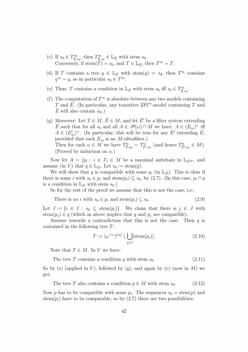
(c) If s0 ∈ T∞E,s0 , then T∞E,s0∈ LE with stem s0.

Conversely, if stem(T ) = s0, and T ∈ LE, then T∞ = T .

(d) If T contains a tree q ∈ LE with stem(q) = s0, then T∞ containsq∞ = q, so in particular s0 ∈ T∞.

(e) Thus: T contains a condition in LE with stem s0 iff s0 ∈ T∞E,s0 .

(f) The computation of T∞ is absolute between any two models containingT and E. (In particular, any transitive ZFC∗-model containing T andE will also contain α0.)

(g) Moreover: Let T ∈M , E ∈M , and let E ′ be a filter system extendingE such that for all s0 and all A ∈ P(ω) ∩M we have: A ∈ (Es0)+ iffA ∈ (E ′s0)+. (In particular, this will be true for any E ′ extending E,provided that each Es0 is an M -ultrafilter.)Then for each α ∈ M we have Tα

E,s0= Tα

E′,s0(and hence Tα

E′,s0∈ M).

(Proved by induction on α.)

Now let A = (pi : i ∈ I) ∈ M be a maximal antichain in LDM , andassume (in V ) that q ∈ LD. Let s0 := stem(q).

We will show that q is compatible with some pi (in LD). This is clear ifthere is some i with s0 ∈ pi and stem(pi) ⊆ s0, by (2.7). (In this case, pi ∩ qis a condition in LD with stem s0.)

So for the rest of the proof we assume that this is not the case, i.e.:

There is no i with s0 ∈ pi and stem(pi) ⊆ s0. (2.9)

Let J := {i ∈ I : s0 ⊆ stem(pi)}. We claim that there is j ∈ J withstem(pj) ∈ q (which as above implies that q and pj are compatible).

Assume towards a contradiction that this is not the case. Then q iscontained in the following tree T :

T := (ω<ω)[s0] \⋃j∈J

[stem(pj)]. (2.10)

Note that T ∈M . In V we have:

The tree T contains a condition q with stem s0. (2.11)

So by (e) (applied in V ), followed by (g), and again by (e) (now in M) weget:

The tree T also contains a condition p ∈M with stem s0. (2.12)

Now p has to be compatible with some pi. The sequences s0 = stem(p) andstem(pi) have to be comparable, so by (2.7) there are two possibilities:

42

1. stem(pi) ⊆ stem(p) = s0 ∈ pi. We have excluded this case in ourassumption (2.9).

2. s0 = stem(p) ⊆ stem(pi) ∈ p. So i ∈ J . By construction of T(see (2.10)), we conclude stem(pi) /∈ T , contradicting stem(pi) ∈ p ⊆ T(see 2.12).

2.1.C Ultralaver kills strong measure zero

The following lemma appears already in [Bla88, Theorem 9]. We will give aproof below in Lemma 2.38.

Lemma 2.13. If A is a finite set,˜α an LD-name, p ∈ LD, and p

˜α ∈ A,

then there is β ∈ A and a pure extension q ≤0 p such that q ˜α = β.

Definition 2.14. Let ¯ be an increasing sequence of natural numbers. Wesay that X ⊆ 2ω is smz with respect to ¯, if there exists a sequence (Ik)k∈ωof basic intervals of 2ω of measure ≤ 2−`k (i.e., each Ik is of the form [sk] forsome sk ∈ 2`k) such that X ⊆

⋂m∈ω

⋃k≥m Ik.

Remark 2.15. It is well known and easy to see that the properties

• For all ¯ there exists a sequence (Ik)k∈ω of basic intervals of 2ω ofmeasure ≤ 2−`k such that X ⊆

⋃k∈ω Ik.

• For all ¯ there exists a sequence (Ik)k∈ω of basic intervals of 2ω ofmeasure ≤ 2−`k such that X ⊆

⋂m∈ω

⋃k≥m Ik.

are equivalent. Hence, a set X is smz iff X is smz with respect to all ¯∈ ωω.

The following lemma is a variant of the corresponding lemma (and proof)for Laver forcing (see for example [Jec03, Lemma 28.20]): Ultralaver makesold uncountable sets non-smz.

Lemma 2.16. Let D be a system of ultrafilters, and let ¯˜` be the LD-name for

the ultralaver real. Then each uncountable set X ∈ V is forced to be non-smz(witnessed by the ultralaver real ¯

˜`).

More precisely, the following holds:

LD ∀X ∈ V ∩ [2ω]ℵ1 ∀(xk)k∈ω ⊆ 2ω X 6⊆⋂m∈ω

⋃k≥m

[xk�˜`k]. (2.17)

We first give two technical lemmas:

43

Lemma 2.18. Let p ∈ LD with stem s ∈ ω<ω, and let˜x be a LD-name for a

real in 2ω. Then there exists a pure extension q ≤0 p and a real τ ∈ 2ω suchthat for every n ∈ ω,

{i ∈ succq(s) : q[s_i] ˜x�n = τ�n} ∈ Ds. (2.19)

Proof. For each i ∈ succp(s), let qi ≤0 p[s_i] be such that qi decides˜x�i,

i.e., there is a ti of length i such that qi ˜x�i = ti (this is possible by

Lemma 2.13).Now we define the real τ ∈ 2ω as the Ds-limit of the ti’s. In more detail:

For each n ∈ ω there is a (unique) τn ∈ 2n such that {i : ti�n = τn} ∈ Ds;since Ds is a filter, there is a real τ ∈ 2ω with τ�n = τn for each n. Finally,let q :=

⋃i qi.

Lemma 2.20. Let p ∈ LD with stem s, and let (˜xk)k∈ω be a sequence of

LD-names for reals in 2ω. Then there exists a pure extension q ≤0 p and afamily of reals (τη)η∈q, η⊇s ⊆ 2ω such that for each η ∈ q above s, and everyn ∈ ω,

{i ∈ succq(η) : q[η_i] ˜x|η|�n = τη�n} ∈ Dη. (2.21)

Proof. We apply Lemma 2.18 to each node η in p above s (and to˜x|η|)

separately: We first get a p1 ≤0 p and a τs ∈ 2ω; for every immediatesuccessor η ∈ succp1(s), we get qη ≤0 p

[η]1 and a τη ∈ 2ω, and let p2 :=

⋃η qη;

in this way, we get a (fusion) sequence (p, p1, p2, . . .), and let q :=⋂k pk.

Proof of Lemma 2.16. We want to prove (2.17). Assume towards a contra-diction that X is an uncountable set in V , and that (

˜xk)k∈ω is a sequence of

names for reals in 2ω and p ∈ LD such that

p X ⊆⋂m∈ω

⋃k≥m

[˜xk�

˜`k]. (2.22)

Let s ∈ ω<ω be the stem of p.By Lemma 2.20, we can fix a pure extension q ≤0 p and a family

(τη)η∈q, η⊇s ⊆ 2ω such that for each η ∈ q above the stem s and every n ∈ ω,condition (2.21) holds.

Since X is (in V and) uncountable, we can find a real x∗ ∈ X which isdifferent from each real in the countable family (τη)η∈q, η⊇s; more specifically,we can pick a family of natural numbers (nη)η∈q, η⊇s such that x∗�nη 6= τη�nηfor any η.

We can now find r ≤0 q such that:

• For all η ∈ r above s and all i ∈ succr(η) we have i > nη.

44

• For all η ∈ r above s and all i ∈ succr(η) we have r[η_i] ˜x|η|�nη =

τη�nη 6= x∗�nη.

So for all η ∈ r above s we have, writing k for |η|, that r[η_i] forces x∗ /∈[˜xk�nη] ⊇ [

˜xk�`k]. We conclude that r forces x∗ /∈

⋃k≥|s|[˜

xk�`k], contradicting

(2.22).

Corollary 2.23. Let (tk)k∈ω be a dense subset of 2ω.Let D be a system of ultrafilters, and let ¯

˜` be the LD-name for the ul-

tralaver real. Then the set

˜H :=

⋂m∈ω

⋃k≥m

[tk�˜`k]

is forced to be a comeager set with the property that˜H does not contain any

translate of any old uncountable set.

Pawlikowski’s theorem 2.2 gives us:

Corollary 2.24. There is a canonical name F for a closed null set such thatX + F is positive for all uncountable X in V .

In particular, no uncountable ground model set is smz in the ultralaverextension.

2.1.D Thin sets and strong measure zero

For the notion of “(very) thin” set, we use an increasing function B∗(k)(the function we use will be described in Corollary 2.56). We will assumethat ¯∗ = (`∗k)k∈ω is an increasing sequence of natural numbers with `∗k+1 �B∗(k). (We will later use a subsequence of the ultralaver real ¯ as ¯∗, seeLemma 2.26).

Definition 2.25. For X ⊆ 2ω and k ∈ ω we write X�[`∗k, `∗k+1) for the set

{x�[`∗k, `∗k+1) : x ∈ X}. We say that

• X ⊆ 2ω is “very thin with respect to ¯∗ and B∗”, if there are infinitelymany k with |X�[`∗k, `∗k+1)| ≤ B∗(k).

• X ⊆ 2ω is “thin with respect to ¯∗ and B∗”, if X is the union ofcountably many very thin sets.

Note that the family of thin sets is a σ-ideal, while the family of verythin sets is not even an ideal. Also, every very thin set is covered by a closedvery thin (in particular nowhere dense) set. In particular, every thin set ismeager and the ideal of thin sets is a proper ideal.

45

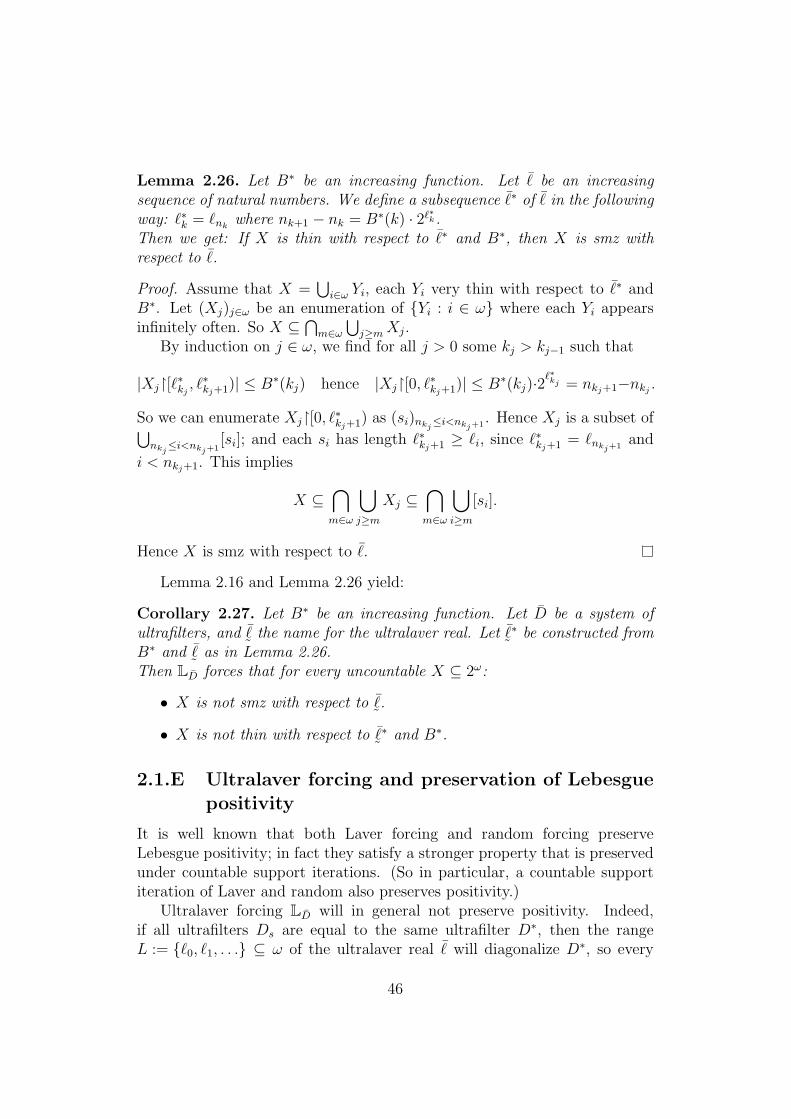
Lemma 2.26. Let B∗ be an increasing function. Let ¯ be an increasingsequence of natural numbers. We define a subsequence ¯∗ of ¯ in the followingway: `∗k = `nk where nk+1 − nk = B∗(k) · 2`∗k .Then we get: If X is thin with respect to ¯∗ and B∗, then X is smz withrespect to ¯.

Proof. Assume that X =⋃i∈ω Yi, each Yi very thin with respect to ¯∗ and

B∗. Let (Xj)j∈ω be an enumeration of {Yi : i ∈ ω} where each Yi appearsinfinitely often. So X ⊆

⋂m∈ω

⋃j≥mXj.

By induction on j ∈ ω, we find for all j > 0 some kj > kj−1 such that

|Xj�[`∗kj, `∗kj+1)| ≤ B∗(kj) hence |Xj�[0, `

∗kj+1)| ≤ B∗(kj)·2

`∗kj = nkj+1−nkj .

So we can enumerate Xj�[0, `∗kj+1) as (si)nkj≤i<nkj+1. Hence Xj is a subset of⋃

nkj≤i<nkj+1[si]; and each si has length `∗kj+1 ≥ `i, since `∗kj+1 = `nkj+1

and

i < nkj+1. This implies

X ⊆⋂m∈ω

⋃j≥m

Xj ⊆⋂m∈ω

⋃i≥m

[si].

Hence X is smz with respect to ¯.

Lemma 2.16 and Lemma 2.26 yield:

Corollary 2.27. Let B∗ be an increasing function. Let D be a system ofultrafilters, and

˜¯ the name for the ultralaver real. Let

˜¯∗ be constructed from

B∗ and˜¯ as in Lemma 2.26.

Then LD forces that for every uncountable X ⊆ 2ω:

• X is not smz with respect to˜¯.

• X is not thin with respect to˜¯∗ and B∗.

2.1.E Ultralaver forcing and preservation of Lebesguepositivity

It is well known that both Laver forcing and random forcing preserveLebesgue positivity; in fact they satisfy a stronger property that is preservedunder countable support iterations. (So in particular, a countable supportiteration of Laver and random also preserves positivity.)

Ultralaver forcing LD will in general not preserve positivity. Indeed,if all ultrafilters Ds are equal to the same ultrafilter D∗, then the rangeL := {`0, `1, . . .} ⊆ ω of the ultralaver real ¯ will diagonalize D∗, so every

46

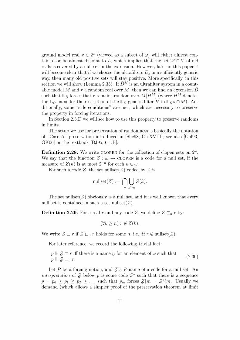
ground model real x ∈ 2ω (viewed as a subset of ω) will either almost con-tain L or be almost disjoint to L, which implies that the set 2ω ∩ V of oldreals is covered by a null set in the extension. However, later in this paper itwill become clear that if we choose the ultrafilters Ds in a sufficiently genericway, then many old positive sets will stay positive. More specifically, in thissection we will show (Lemma 2.33): If DM is an ultrafilter system in a count-able model M and r a random real over M , then we can find an extension Dsuch that LD forces that r remains random over M [HM ] (where HM denotesthe LD-name for the restriction of the LD-generic filter H to LDM ∩M). Ad-ditionally, some “side conditions” are met, which are necessary to preservethe property in forcing iterations.

In Section 2.3.D we will see how to use this property to preserve randomsin limits.

The setup we use for preservation of randomness is basically the notationof “Case A” preservation introduced in [She98, Ch.XVIII], see also [Gol93,GK06] or the textbook [BJ95, 6.1.B]:

Definition 2.28. We write clopen for the collection of clopen sets on 2ω.We say that the function Z : ω → clopen is a code for a null set, if themeasure of Z(n) is at most 2−n for each n ∈ ω.

For such a code Z, the set nullset(Z) coded by Z is

nullset(Z) :=⋂n

⋃k≥n

Z(k).

The set nullset(Z) obviously is a null set, and it is well known that everynull set is contained in such a set nullset(Z).

Definition 2.29. For a real r and any code Z, we define Z @n r by:

(∀k ≥ n) r /∈ Z(k).

We write Z @ r if Z @n r holds for some n; i.e., if r /∈ nullset(Z).

For later reference, we record the following trivial fact:

p ˜Z @ r iff there is a name

˜n for an element of ω such that

p ˜Z @

˜n r.

(2.30)

Let P be a forcing notion, and˜Z a P -name of a code for a null set. An

interpretation of˜Z below p is some code Z∗ such that there is a sequence

p = p0 ≥ p1 ≥ p2 ≥ . . . such that pm forces˜Z�m = Z∗�m. Usually we

demand (which allows a simpler proof of the preservation theorem at limit

47

stages) that the sequence (p0, p1, . . . ) is inconsistent, i.e., p forces that thereis an m such that pm /∈ G. Note that whenever P adds a new ω-sequence ofordinals, we can find such an interpretation for any

˜Z.

If˜Z = (

˜Z1, . . . ,

˜Zm) is a tuple of names of codes for null sets, then an

interpretation of ¯˜Z below p is some tuple (Z∗1 , . . . , Z

∗m) such that there is a

single sequence p = p0 ≥ p1 ≥ p2 ≥ . . . interpreting each˜Zi as Z∗i .

We now turn to preservation of Lebesgue positivity:

Definition 2.31. 1. A forcing notion P preserves Borel outer measure,if P forces Leb∗(AV ) = Leb(AV [GP ]) for every code A for a Borel set.(Leb∗ denotes the outer Lebesgue measure, and for a Borel code A anda set-theoretic universe V , AV denotes the Borel set coded by A in V .)

2. P strongly preserves randoms, if the following holds: Let N ≺ H(χ∗)be countable for a sufficiently large regular cardinal χ∗, let P, p, ¯

˜Z =

(˜Z1, . . . ,

˜Zm) ∈ N , let p ∈ P and let r be random over N . Assume that

in N , Z∗ is an interpretation of˜Z, and assume Z∗i @ki r for each i. Then

there is an N -generic q ≤ p forcing that r is still random over N [G]and moreover,

˜Zi @ki r for each i. (In particular, P has to be proper.)

3. Assume that P is absolutely definable. P strongly preserves randomsover countable models if (2) holds for all countable (transitive10) modelsN of ZFC∗.

It is easy to see that these properties are increasing in strength. (Ofcourse (3)⇒(2) works only if ZFC∗ is satisfied in H(χ∗).)

In [KS05] it is shown that (1) implies (3), provided that P is nep (“non-elementary proper”, i.e., nicely definable and proper with respect to count-able models). In particular, every Suslin ccc forcing notion such as randomforcing, and also many tree forcing notions including Laver forcing, are nep.However LD is not nicely definable in this sense, as its definition uses ultra-filters as parameters.

Lemma 2.32. Both Laver forcing and random forcing strongly preserve ran-doms over countable models.

Proof. For random forcing, this is easy and well known (see, e.g., [BJ95,6.3.12]).

For Laver forcing: By the above, it is enough to show (1). This was doneby Woodin (unpublished) and Judah-Shelah [JS90]. A nicer proof (includinga variant of (2)) is given by Pawlikowski [Paw96c].

10Later we will introduce ord-transitive models, and it is easy to see that it does not makeany difference whether we demand transitive or not; this can be seen using a transitivecollapse.

48

Ultralaver will generally not preserve Lebesgue positivity, let alone ran-domness. However, we get the following “local” variant of strong preservationof randoms (which will be used in the preservation theorem 2.109). The restof this section will be devoted to the proof of the following lemma.

Lemma 2.33. Assume that M is a countable model, DM an ultrafilter systemin M and r a random real over M . Then there is (in V ) an ultrafilter systemD extending11 DM , such that the following holds:If

• p ∈ LDM ,

• in M ,˜Z = (

˜Z1, . . . ,

˜Zm) is a sequence of LDM -names for codes for

null sets,12 and Z∗1 , . . . , Z∗m are interpretations under p, witnessed by a

sequence (pn)n∈ω with strictly increasing13 stems,

• Z∗i @ki r for i = 1, . . . ,m,

then there is a q ≤ p in LD forcing that

• r is random over M [GM ],

•˜Zi @ki r for i = 1, . . . ,m.

For the proof of this lemma, we will use the following concepts:

Definition 2.34. Let p ⊆ ω<ω be a tree. A “front name below p” is afunction14 h : F → clopen, where F ⊆ p is a front (a set that meets everybranch of p in a unique point). (For notational simplicity we also allow h tobe defined on elements /∈ p; this way, every front name below p is also a frontname below q whenever q ≤ p.)

If h is a front name and D is any filter system with p ∈ LD, we definethe corresponding LD-name (in the sense of forcing)

˜zh by

˜zh := {(y, p[s]) : s ∈ F, y ∈ h(s)}. (2.35)

(This does not depend on the D we use, since we set y := {(x, ω<ω) : x ∈ y}.)Up to forced equality, the name

˜zh is characterized by the fact that p[s]

forces (in any LD) that˜zh = h(s), for every s in the domain of h.

11This implies, by Lemma 2.8, that the LD-generic filter G induces an LDM -genericfilter over M , which we call GM .

12Recall that nullset(˜Z) =

⋂n

⋃k≥n ˜

Z(k) is a null set in the extension.13It is enough to assume that the lengths of the stems diverge to infinity; any thin

enough subsequence will then have strictly increasing stems and will still interpret each

˜Zi as Z∗i .

14Instead of clopen we may also consider other ranges of front names, such as the classof all ordinals, or the set ω.

49

Note that the same object h can be viewed as a front name below p withrespect to different forcings LD1

, LD2, as long as p ∈ LD1

∩ LD2.

Definition 2.36. Let p ⊆ ω<ω be a tree. A “continuous name below p” iseither of the following:

• An ω-sequence of front names below p.

• A ⊆-increasing function g : p→ clopen<ω such thatlimn→∞ lh(g(c�n)) =∞ for every branch c ∈ [p].

For each n, the set of minimal elements in {s ∈ p : lh(g(s)) > n} is a front,so each continuous name in the second sense naturally defines a name in thefirst sense, and conversely. Being a continuous name below p does not involvethe notion of nor does it depend on the filter system D.

If g is a continuous name and D is any filter system, we can again definethe corresponding LD-name

˜Zg (in the sense of forcing); we leave a formal

definition of˜Zg to the reader and content ourselves with this characterization:

(∀s ∈ p) : p[s] LD g(s) ⊆˜Zg. (2.37)

Note that a continuous name below p naturally corresponds to a contin-uous function F : [p]→ clopenω, and

˜Zg is forced (by p) to be the value of

F at the generic real˜¯.

Lemma 2.38. LD has the following “pure decision properties”:

1. Whenever˜y is a name for an element of clopen, p ∈ LD, then there

is a pure extension p1 ≤0 p such that˜y =

˜zh (is forced) for a front

name h below p1.

2. Whenever˜Y is a name for a sequence of elements of clopen, p ∈ LD,

then there is a pure extension q ≤0 p such that˜Y =

˜Zg (is forced) for

some continuous name g below q.

3. (This is Lemma 2.13.) If A is a finite set,˜α a name, p ∈ LD, and p

forces˜α ∈ A, then there is β ∈ A and a pure extension q ≤0 p such

that q ˜α = β.

Proof. Let p ∈ LD, s0 := stem(p),˜y a name for an element of clopen.

We call t ∈ p a “good node in p” if˜y is a front name below p[t] (more

formally: forced to be equal to˜zh for a front name h). We can find p1 ≤0 p

such that for all t ∈ p1 above s0: If there is q ≤0 p[t]1 such that t is good in q,

then t is already good in p1.

50

We claim that s0 is now good (in p1). Note that for any bad node sthe set { t ∈ succp1(s) : t bad } is in D+

s . Hence, if s0 is bad, we caninductively construct p2 ≤0 p1 such that all nodes of p2 are bad nodes in p1.Now let q ≤ p2 decide

˜y, s := stem(q). Then q ≤0 p

[s]1 , so s is good in p1,

contradiction. This finishes the proof of (1).To prove (2), we first construct p1 as in (1) with respect to

˜y0. This

gives a front F1 ⊆ p1 deciding˜y0. Above each node in F1 we now repeat the

construction from (1) with respect to˜y1, yielding p2, etc. Finally, q :=

⋂n pn.

To prove (3): Similar to (1), we can find p1 ≤0 p such that for each t ∈ p1:

If there is a pure extension of p[t]1 deciding

˜α, then p

[t]1 decides

˜α; in this case

we again call t good. Since there are only finitely many possibilities for thevalue of

˜α, any bad node t has D+

t many bad successors. So if the stem ofp1 is bad, we can again reach a contradiction as in (1).

Corollary 2.39. Let D be a filter system, and let G ⊆ LD be generic. Thenevery Y ∈ clopenω in V [G] is the evaluation of a continuous name

˜Zg by

G.

Proof. In V , fix a p ∈ LD and a name˜Y for an element of clopenω. We

can find q ≤0 p and a continuous name g below q such that q ˜Y =

˜Zg.

We will need the following modification of the concept of “continuousnames”.

Definition 2.40. Let p ⊆ ω<ω be a tree, b ∈ [p] a branch. An “almostcontinuous name below p (with respect to b)” is a ⊆-increasing function g :p → clopen<ω such that limn→∞ lh(g(c�n)) = ∞ for every branch c ∈ [p],except possibly for c = b.

Note that “except possibly for c = b” is the only difference between thisdefinition and the definition of a continuous name.

Since for any D it is forced15 that the generic real (for LD) is not equal tothe exceptional branch b, we again get a name

˜Zg of a function in clopenω

satisfying:(∀s ∈ p) : p[s] LD g(s) ⊆

˜Zg.

An almost continuous name naturally corresponds to a continuous functionF from [p] \ {b} into clopenω.

Note that being an almost continuous name is a very simple combinatorialproperty of g which does not depend on D, nor does it involve the notion .Thus, the same function g can be viewed as an almost continuous name fortwo different forcing notions LD1

, LD2simultaneously.

15This follows from our assumption that all our filters contain the Frechet filter.

51

Lemma 2.41. Let D be a system of filters (not necessarily ultrafilters).Assume that p = (pn)n∈ω witnesses that Y ∗ is an interpretation of

˜Y , and

that the lengths of the stems of the pn are strictly increasing.16 Then thereexists a sequence q = (qn)n∈ω such that

1. q0 ≥ q1 ≥ · · · .

2. qn ≤ pn for all n.

3. q also interprets˜Y as Y ∗. (This follows from the previous two state-

ments.)

4.˜Y is almost continuous below q0, i.e., there is an almost continuousname g such that q0 forces

˜Y =

˜Zg.

5.˜Y is almost continuous below qn, for all n. (This follows from theprevious statement.)

Proof. Let b be the branch described by the stems of the conditions pn:

b := {s : (∃n) s ⊆ stem(pn)}.

We now construct a condition q0. For every s ∈ b satisfying stem(pn) ⊆s ( stem(pn+1) we set succq0(s) = succpn(s), and for all t ∈ succq0(s) except

for the one in b we let q[t]0 ≤0 p

[t]n be such that

˜Y is continuous below q

[t]0 . We

can do this by Lemma 2.38(2).Now we set

qn := pn ∩ q0 = q[stem(pn)]0 ≤ pn.

This takes care of (1) and (2). Now we show (4): Any branch c of q0 not

equal to b must contain a node s_k /∈ b with s ∈ b, so c is a branch in q[s_k]0 ,

below which˜Y was continuous.

The following lemmas and corollaries are the motivation for consideringcontinuous and almost continuous names.

Lemma 2.42. Let D be a system of filters (not necessarily ultrafilters). Letp ∈ LD, let b be a branch, and let g : p→ clopen<ω be an almost continuousname below p with respect to b; write

˜Zg for the associated LD-name.

Let r ∈ 2ω be a real, n0 ∈ ω. Then the following are equivalent:

1. p LD r /∈⋃n≥n0 ˜

Zg(n), i.e.,˜Zg @n0 r.

16It is easy to see that for every LD-name˜Y we can find such p and Y ∗: First find p

which interprets both˜Y and ¯

˜`, and then thin out to get a strictly increasing sequence of

stems.

52

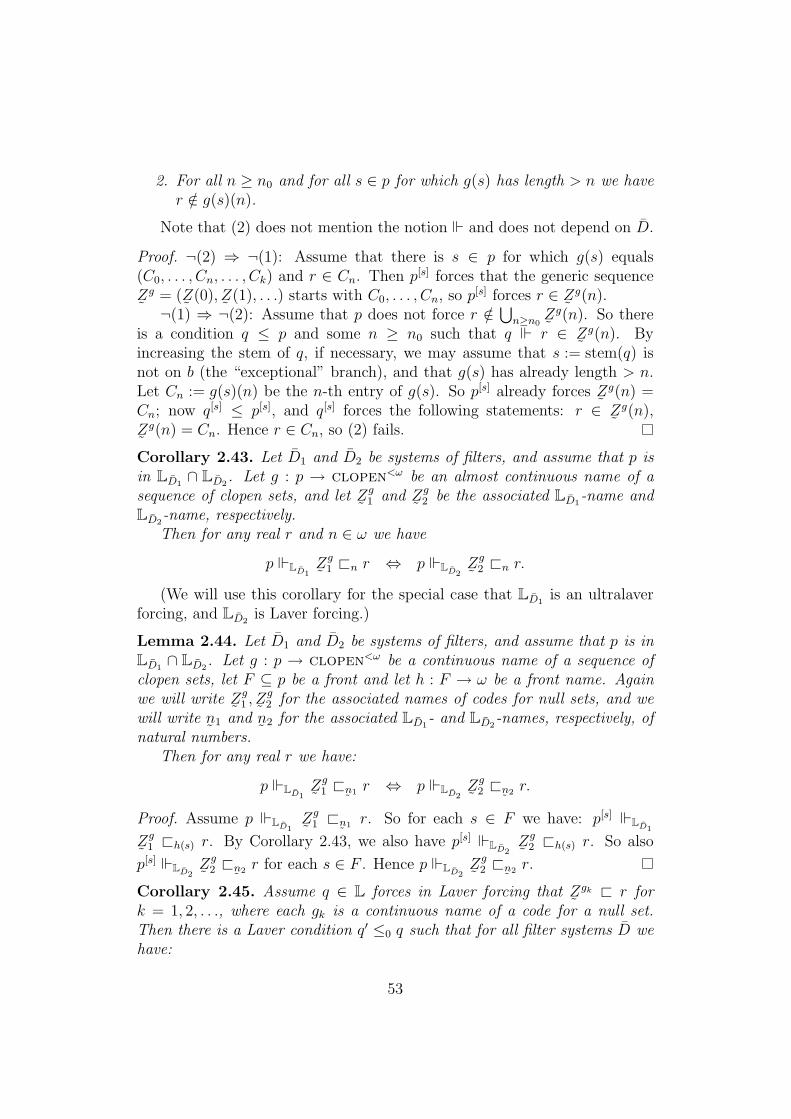
2. For all n ≥ n0 and for all s ∈ p for which g(s) has length > n we haver /∈ g(s)(n).

Note that (2) does not mention the notion and does not depend on D.

Proof. ¬(2) ⇒ ¬(1): Assume that there is s ∈ p for which g(s) equals(C0, . . . , Cn, . . . , Ck) and r ∈ Cn. Then p[s] forces that the generic sequence

˜Zg = (

˜Z(0),

˜Z(1), . . .) starts with C0, . . . , Cn, so p[s] forces r ∈

˜Zg(n).

¬(1) ⇒ ¬(2): Assume that p does not force r /∈⋃n≥n0 ˜

Zg(n). So thereis a condition q ≤ p and some n ≥ n0 such that q r ∈

˜Zg(n). By

increasing the stem of q, if necessary, we may assume that s := stem(q) isnot on b (the “exceptional” branch), and that g(s) has already length > n.Let Cn := g(s)(n) be the n-th entry of g(s). So p[s] already forces

˜Zg(n) =

Cn; now q[s] ≤ p[s], and q[s] forces the following statements: r ∈˜Zg(n),

˜Zg(n) = Cn. Hence r ∈ Cn, so (2) fails.

Corollary 2.43. Let D1 and D2 be systems of filters, and assume that p isin LD1

∩ LD2. Let g : p → clopen<ω be an almost continuous name of a

sequence of clopen sets, and let˜Zg

1 and˜Zg

2 be the associated LD1-name and

LD2-name, respectively.Then for any real r and n ∈ ω we have

p LD1 ˜Zg

1 @n r ⇔ p LD2 ˜Zg

2 @n r.

(We will use this corollary for the special case that LD1is an ultralaver

forcing, and LD2is Laver forcing.)

Lemma 2.44. Let D1 and D2 be systems of filters, and assume that p is inLD1∩ LD2

. Let g : p → clopen<ω be a continuous name of a sequence ofclopen sets, let F ⊆ p be a front and let h : F → ω be a front name. Againwe will write

˜Zg

1 ,˜Zg

2 for the associated names of codes for null sets, and wewill write

˜n1 and

˜n2 for the associated LD1

- and LD2-names, respectively, of

natural numbers.Then for any real r we have:

p LD1 ˜Zg

1 @˜n1 r ⇔ p LD2 ˜

Zg2 @

˜n2 r.

Proof. Assume p LD1 ˜Zg

1 @˜n1 r. So for each s ∈ F we have: p[s] LD1

˜Zg

1 @h(s) r. By Corollary 2.43, we also have p[s] LD2 ˜Zg

2 @h(s) r. So also

p[s] LD2 ˜Zg

2 @˜n2 r for each s ∈ F . Hence p LD2 ˜

Zg2 @

˜n2 r.

Corollary 2.45. Assume q ∈ L forces in Laver forcing that˜Zgk @ r for

k = 1, 2, . . ., where each gk is a continuous name of a code for a null set.Then there is a Laver condition q′ ≤0 q such that for all filter systems D wehave:

53

If q′ ∈ LD, then q′ forces (in ultralaver forcing LD) that˜Zgk @ r

for all k.

Proof. By (2.30) we can find a sequence (˜nk)∞k=1 of L-names such that q

˜Zgk @

˜nk r for each k. By Lemma 2.38(2) we can find q′ ≤0 q such that this

sequence is continuous below q′. Since each˜nk is now a front name below q′,

we can apply the previous lemma.

Lemma 2.46. Let M be a countable model, r ∈ 2ω, DM ∈ M an ultrafiltersystem, D a filter system extending DM , q ∈ LD. For any V -generic filterG ⊆ LD we write GM for the (M-generic, by Lemma 2.8) filter on LDM .

The following are equivalent:

1. q LD r is random over M [GM ].

2. For all names˜Z ∈M of codes for null sets: q LD ˜

Z @ r.

3. For all continuous names g ∈M : q LD ˜Zg @ r.

Proof. (1)⇔(2) holds because every null set is contained in a set of the formnullset(Z), for some code Z.

(2)⇔(3): Every code for a null set in M [GM ] is equal to˜Zg[GM ], for some

g ∈M , by Corollary 2.39.

The following lemma may be folklore. Nevertheless, we prove it for theconvenience of the reader.

Lemma 2.47. Let r be random over a countable model M and A ∈M . Thenthere is a countable model M ′ ⊇ M such that A is countable in M ′, but r isstill random over M ′.

Proof. We will need the following forcing notions, all defined in M :

MC //

B1

��

MC

˜B2

��MB1

˜P=C∗

˜B2/B1

// MC∗˜B2

• Let C be the forcing that collapses the cardinality of A to ω with finiteconditions.

• Let B1 be random forcing (trees T ⊆ 2<ω of positive measure).

• Let˜B2 be the C-name of random forcing.

54

• Let i : B1 → C ∗˜B2 be the natural complete embedding T 7→ (1C , T ).

• Let˜P be a B1-name for the forcing C∗

˜B2/i[GB1 ], the quotient of C∗

˜B2

by the complete subforcing i[B1].

The random real r is B1-generic over M . In M [r] we let P :=˜P [r]. Now

let H ⊆ P be generic over M [r]. Then r ∗ H ⊆ B1 ∗˜P ' C ∗

˜B2 induces

an M -generic filter J ⊆ C and an M [J ]-generic filter K ⊆˜B2[J ]; it is easy

to check that K interprets the˜B2-name of the canonical random real as the

given random real r.Hence r is random over the countable model M ′ := M [J ], and A is count-

able in M ′.

MJ //

r

��

M [J ]

K��

M [r]H

// M [r][H]

Proof of Lemma 2.33. We will first describe a construction that deals witha single triple (p, ¯

˜Z, Z∗) (where p is a sequence of conditions with strictly

increasing stems which interprets ¯˜Z as Z∗); this construction will yield a

condition q′ = q′(p, ¯˜Z, Z∗). We will then show how to deal with all possible

triples.So let p be a condition, and let p = (pk)k∈ω be a sequence interpreting ¯

˜Z

as Z∗, where the lengths of the stems of pn are strictly increasing and p0 = p.It is easy to see that it is enough to deal with a single null set, i.e., m = 1,and with k1 = 0. We write

˜Z and Z∗ instead of

˜Z1 and Z∗1 .

Using Lemma 2.41 we may (strengthening the conditions in our inter-pretation) assume (in M) that the sequence (

˜Z(k))k∈ω is almost continuous,

witnessed by g : p → clopen<ω. By Lemma 2.47, we can find a modelM ′ ⊇M such that (2ω)M is countable in M ′, but r is still random over M ′.

We now work in M ′. Note that g still defines an almost continuous name,which we again call

˜Z.

Each filter in DMs is now countably generated; let As be a pseudo-

intersection of DMs which additionally satisfies As ⊆ succp(s) for all s ∈ p

above the stem. Let D′s be the Frechet filter on As. Let p′ ∈ LD′ be the treewith the same stem as p which satisfies succp′(s) = As for all s ∈ p′ abovethe stem.

By Lemma 2.8, we know that LDM is an M -complete subforcing of LD′(in M ′ as well as in V ). We write GM for the induced filter on LDM .

55

We now work in V . Note that below the condition p′, the forcing LD′is just Laver forcing L, and that p′ ≤L p. Using Lemma 2.32 we can find acondition q ≤ p′ (in Laver forcing L) such that:

q is M ′-generic. (2.48)

q L r is random over M ′[GL] (hence also over M [GM ]). (2.49)

Moreover, q L˜Z @0 r. (2.50)

Enumerate all continuous LDM -names of codes for null sets from M as

˜Zg1 ,

˜Zg2 , . . . Applying Corollary 2.45 yields a condition q′ ≤ q such that for

all filter systems E satisfying q′ ∈ LE, we have q′ LE ˜Zgi @ r for all i.

Corollary 2.43 and Lemma 2.46 now imply:

For every filter system E satisfying q′ ∈ LE, q′ forces in LEthat r is random over M [GM ] and that

˜Z @0 r.

(2.51)

By thinning out q′ we may assume that

For each ν ∈ ωω ∩M there is k such that ν�k /∈ q′. (2.52)

We have now described a construction of q′ = q′(p,˜Z,Z∗).

Let (pn,˜Zn, Z∗n) enumerate all triples (p,

˜Z,Z∗) ∈ M where p interprets

˜Z as Z∗ (and consists of conditions with strictly increasing stems). For each nwrite νn for

⋃k stem(pnk), the branch determined by the stems of the sequence

pn. We now define by induction a sequence qn of conditions:

• q0 := q′(p0,˜Z0, Z∗0).

• Given qn−1 and (pn,˜Zn, Z∗n), we find k0 such that νn�k0 /∈ q0∪· · ·∪qn−1

(using (2.52)). Let k1 be such that stem(pnk1) has length > k0. We

replace pn by p′ := (pnk)k≥k1 . (Obviously, p′ still interprets˜Zn as Z∗n.)

Now let qn := q′(p′,˜Zn, Z∗n).

Note that the stem of qn is at least as long as the stem of pnk1, and is therefore

not in q0∪ · · · ∪ qn−1, so stem(qi) and stem(qj) are incompatible for all i 6= j.Therefore we can choose for each s an ultrafilter Ds extending DM

s such thatstem(qi) ⊆ s implies succqi(s) ∈ Ds.

Note that all qi are in LD. Therefore, we can use (2.51). Also, qi ≤ pi0.

Below, in Lemma 2.109, we will prove a preservation theorem using thefollowing “local” variant of “random preservation”:

56

Definition 2.53. Fix a countable model M , a real r ∈ 2ω and a forcingnotion QM ∈ M . Let QM be an M -complete subforcing of Q. We say that“Q locally preserves randomness of r over M”, if there is in M a sequence(DQM

n )n∈ω of open dense subsets of QM such that the following holds:Assume that

• M thinks that p := (pn)n∈ω interprets (˜Z1, . . . ,

˜Zm) as (Z∗1 , . . . , Z

∗m) (so

each˜Zi is a QM -name of a code for a null set and each Z∗i is a code for

a null set, both in M);

• moreover, each pn is in DQM

n (we call such a sequence (pn)n∈ω, or theaccording interpretation, “quick”);

• r is random over M ;

• Z∗i @ki r for i = 1, . . . ,m.

Then there is a q ≤Q p0 forcing that

• r is random over M [GM ];

•˜Zi @ki r for i = 1, . . . ,m.

Note that this is trivially satisfied if r is not random over M .For a variant of this definition, see Section 2.6.Setting DQM

n to be the set of conditions with stem of length at least n,Lemma 2.33 gives us:

Corollary 2.54. If QM is an ultralaver forcing in M and r a real, thenthere is an ultralaver forcing Q over17 QM locally preserving randomness ofr over M .

2.2 Janus forcing

In this section, we define a family of forcing notions that has two faces (hencethe name “Janus forcing”): Elements of this family may be countable (andtherefore equivalent to Cohen), and they may also be essentially random.

In the rest of the paper, we will use the following properties of Janusforcing notions J. (And we will use only these properties. So readers whoare willing to take these properties for granted could skip to Section 2.3.)

Throughout the whole paper we fix a function B∗ : ω → ω given byCorollary 2.56. The Janus forcings will depend on a real parameter ¯∗ =

17“Q over QM” just means that QM is an M -complete subforcing of Q.

57

(`∗m)m∈ω ∈ ωω which grows fast with respect to B∗. (In our application, ¯∗

will be given by a subsequence of an ultralaver real.)The sequence ¯∗ and the function B∗ together define a notion of a “thin

set” (see Definition 2.25).

1. There is a canonical J-name for a (code for a) null set˜Z∇.

Whenever X ⊆ 2ω is not thin, and J is countable, then J forces that Xis not strongly meager, witnessed18 by nullset(

˜Z∇) (the set we get when

we evaluate the code˜Z∇). Moreover, for any J-name

˜Q of a σ-centered

forcing, also J∗˜Q forces that X is not strongly meager, again witnessed

by nullset(˜Z∇).

(This is Lemma 2.63; “thin” is defined in Definition 2.25.)

2. Let M be a countable transitive model and JM a Janus forcing in M .Then JM is a Janus forcing in V as well (and of course countable in V ).(Also note that trivially the forcing JM is an M -complete subforcing ofitself.)(This is Fact 2.62.)

3. Whenever M is a countable transitive model and JM is a Janus forcingin M , then there is a Janus forcing J such that

• JM is an M -complete subforcing of J.• J is (in V ) equivalent to random forcing (actually we just need thatJ preserves Lebesgue positivity in a strong and iterable way).

(This is Lemma 2.70 and Lemma 2.74.)

4. Moreover, the name˜Z∇ referred to in (1) is so “canonical” that it

evaluates to the same code in the J-generic extension over V as in theJM -generic extension over M .(This is Fact 2.61.)

2.2.A Definition of Janus

A Janus forcing J will consist of:19

• A countable “core” (or: backbone) ∇ which is defined in a combinato-rial way from a parameter ¯∗. (In our application, we will use a Janus

18in the sense of (2.1)19We thank Andreas Blass and Jindrich Zapletal for their comments that led to an

improved presentation of Janus forcing.

58

forcing immediately after an ultralaver forcing, and ¯∗ will be a sub-sequence of the ultralaver real.) This core is of course equivalent toCohen forcing.

• Some additional “stuffing” J \ ∇ (countable20 or uncountable). Weallow great freedom for this, we just require that the core ∇ is a “suf-ficiently” complete subforcing (in a specific combinatorial sense, seeDefinition 2.59(3)).

We will use the following combinatorial theorem from [BS10]:

Lemma 2.55 ([BS10, Theorem 8]21). For every ε, δ > 0 there exists Nε,δ ∈ ωsuch that for all sufficiently large finite sets I ⊆ ω there is a family AI with

|AI | ≥ 2 consisting of sets A ⊆ 2I with|A|2|I|≤ ε such that if X ⊆ 2I ,

|X| ≥ Nε,δ then|{A ∈ AI : X + A = 2I}|

|AI |≥ 1− δ.

(Recall that X + A := {x+ a : x ∈ X, a ∈ A}.)

Rephrasing and specializing to δ = 14

and ε = 12i

we get:

Corollary 2.56. For every i ∈ ω there exists B∗(i) such that for all finitesets I with |I| ≥ B∗(i) there is a nonempty family AI with |AI | ≥ 2 satisfyingthe following:

• AI consists of sets A ⊆ 2I with|A|2|I|≤ 1

2i.

• For every X ⊆ 2I satisfying |X| ≥ B∗(i), the set {A ∈ AI : X+A = 2I}has at least 3

4|AI | elements.

Assumption 2.57. We fix a sufficiently fast increasing sequence ¯∗ = (`∗i )i∈ωof natural numbers; more precisely, the sequence ¯∗ will be a subsequence ofan ultralaver real ¯, defined as in Lemma 2.26 using the function B∗ fromCorollary 2.56. Note that in this case `∗i+1 − `∗i ≥ B∗(i); so we can fix foreach i a family Ai ⊆ P(2Li) on the interval Li := [`∗i , `

∗i+1) according to

Corollary 2.56.

20Also the trivial case J = ∇ is allowed.21The theorem in [BS10] actually says “for a sufficiently large I”, but the proof shows

that this should be read as “for all sufficiently large I”. Also, the quoted theorem onlyclaims that AI will be nonempty, but for ε ≤ 1

2 and |I| > Nε,δ it is easy to see that AIcannot be a singleton {A}: The set X := 2I \ A has size ≥ 2|I|−1 ≥ Nε,δ but satisfiesX +A 6= 2I , as the constant sequence 0 is not in X +A.

59

Definition 2.58. First we define the “core” ∇ = ∇¯∗ of our forcing:

∇ =⋃i∈ω

∏j<i

Aj.

In other words, σ ∈ ∇ iff σ = (A0, . . . , Ai−1) for some i ∈ ω, A0 ∈ A0, . . . ,Ai−1 ∈ Ai−1. We will denote the number i by height(σ).

The forcing notion ∇ is ordered by reverse inclusion (i.e., end extension):τ ≤ σ if τ ⊇ σ.

Definition 2.59. Let ¯∗ = (`∗i )i∈ω be as in the assumption above. We saythat J is a Janus forcing based on ¯∗ if:

1. (∇,⊇) is an incompatibility-preserving subforcing of J.

2. For each i ∈ ω the set {σ ∈ ∇ : height(σ) = i} is predense in J. Soin particular, J adds a branch through ∇. The union of this branch iscalled

˜C∇ = (

˜C∇0 ,

˜C∇1 ,

˜C∇2 , . . .), where

˜C∇i ⊆ 2Li with

˜C∇i ∈ Ai.

3. “Fatness”:22 For all p ∈ J and all real numbers ε > 0 there are arbitrar-ily large i ∈ ω such that there is a core condition σ = (A0, . . . , Ai−1) ∈∇ (of length i) with

|{A ∈ Ai : σ_A 6⊥J p }||Ai|

≥ 1− ε.

(Recall that p 6⊥J q means that p and q are compatible in J.)

4. J is ccc.

5. J is separative.23

6. (To simplify some technicalities:) J ⊆ H(ℵ1).

We now define˜Z∇, which will be a canonical J-name of (a code for) a

null set. We will use the sequence˜C∇ added by J (see Definition 2.59(2)).

Definition 2.60. Each˜C∇i defines a clopen set

˜Z∇i = {x ∈ 2ω : x�Li ∈

˜C∇i }

of measure at most 12i

. The sequence˜Z∇ = (

˜Z∇0 ,

˜Z∇1 ,

˜Z∇2 , . . .) is (a name for)

a code for the null set

nullset(˜Z∇) =

⋂n<ω

⋃i≥n ˜

Z∇i .

22This is the crucial combinatorial property of Janus forcing. Actually, (3) implies (2).23Separative is defined on page 36.

60

Since˜C∇ is defined “canonically” (see in particular Definition 2.59(1),(2)),

and˜Z∇ is constructed in an absolute way from

˜C∇, we get:

Fact 2.61. If J is a Janus forcing, M a countable model and JM a Janusforcing in M which is an M -complete subset of J, if H is J-generic over Vand HM the induced JM -generic filter over M , then

˜C∇ evaluates to the same

real in M [HM ] as in V [H], and therefore˜Z∇ evaluates to the same code (but

of course not to the same set of reals).

For later reference, we record the following trivial fact:

Fact 2.62. Being a Janus forcing is absolute. In particular, if V ⊆ W are settheoretical universes and J is a Janus forcing in V , then J is a Janus forcingin W . In particular, if M is a countable model in V and J ∈ M a Janusforcing in M , then J is also a Janus forcing in V .Let (Mn)n∈ω be an increasing sequence of countable models, and let Jn ∈Mn

be Janus forcings. Assume that Jn is Mn-complete in Jn+1. Then⋃n Jn is a

Janus forcing, and an Mn-complete extension of Jn for all n.

2.2.B Janus and strongly meager

Carlson [Car93] showed that Cohen reals make every uncountable set X ofthe ground model not strongly meager in the extension (and that not beingstrongly meager is preserved in a subsequent forcing with precaliber ℵ1). Weshow that a countable Janus forcing J does the same (for a subsequent forcingthat is even σ-centered, not just precaliber ℵ1). This sounds trivial, sinceany (nontrivial) countable forcing is equivalent to Cohen forcing anyway.However, we show (and will later use) that the canonical null set

˜Z∇ defined

above witnesses that X is not strongly meager (and not just some null setthat we get out of the isomorphism between J and Cohen forcing). The pointis that while ∇ is not a complete subforcing of J, the condition (3) of theDefinition 2.59 guarantees that Carlson’s argument still works, if we assumethat X is non-thin (not just uncountable). This is enough for us, since byCorollary 2.27 ultralaver forcing makes any uncountable set non-thin.

Recall that we fixed the increasing sequence ¯∗ = (`∗i )i∈ω and B∗. In thefollowing, whenever we say “(very) thin” we mean “(very) thin with respectto ¯∗ and B∗” (see Definition 2.25).

Lemma 2.63. If X is not thin, J is a countable Janus forcing based on ¯∗,and

˜R is a J-name for a σ-centered forcing notion, then J ∗

˜R forces that X

is not strongly meager witnessed by the null set˜Z∇.

61

Proof. Let˜c be a J-name for a function

˜c :

˜R → ω witnessing that

˜R is

σ-centered.Recall that “

˜Z∇ witnesses that X is not strongly meager” means that

X +˜Z∇ = 2ω. Assume towards a contradiction that (p, r) ∈ J ∗

˜R forces that

X+˜Z∇ 6= 2ω. Then we can fix a (J∗

˜R)-name

˜ξ such that (p, r)

˜ξ /∈ X+

˜Z∇,

i.e., (p, r) (∀x ∈ X)˜ξ /∈ x+

˜Z∇. By definition of

˜Z∇, we get

(p, r) (∀x ∈ X) (∃n ∈ ω) (∀i ≥ n)˜ξ�Li /∈ x�Li +

˜C∇i .

For each x ∈ X we can find (px, rx) ≤ (p, r) and natural numbers nx ∈ ωand mx ∈ ω such that px forces that

˜c(rx) = mx and

(px, rx) (∀i ≥ nx)˜ξ�Li /∈ x�Li +

˜C∇i .

So X =⋃p∈J,m∈ω,n∈ωXp,m,n, where Xp,m,n is the set of all x with px = p,

mx = m, nx = n. (Note that J is countable, so the union is countable.) AsX is not thin, there is some p∗,m∗, n∗ such that X∗ := Xp∗,m∗,n∗ is not verythin. So we get for all x ∈ X∗:

(p∗, rx) (∀i ≥ n∗)˜ξ�Li /∈ x�Li +

˜C∇i . (2.64)

Since X∗ is not very thin, there is some i0 ∈ ω such that for all i ≥ i0

the (finite) set X∗�Li has more than B∗(i) elements. (2.65)

Due to the fact that J is a Janus forcing (see Definition 2.59 (3)), there arearbitrarily large i ∈ ω such that there is a core condition σ = (A0, . . . , Ai−1) ∈∇ with

|{A ∈ Ai : σ_A 6⊥J p∗}|

|Ai|≥ 2

3. (2.66)

Fix such an i larger than both i0 and n∗, and fix a condition σ satisfy-ing (2.66).

We now consider the following two subsets of Ai:

{A ∈ Ai : σ_A 6⊥J p∗} and {A ∈ Ai : X∗�Li + A = 2Li}. (2.67)

By (2.66), the relative measure (in Ai) of the left one is at least 23; due

to (2.65) and the definition of Ai according to Corollary 2.56, the relativemeasure of the right one is at least 3

4; so the two sets in (2.67) are not disjoint,

and we can pick an A belonging to both.Clearly, σ_A forces (in J) that

˜C∇i is equal to A. Fix q ∈ J witnessing

σ_A 6⊥J p∗. Then

q J X∗�Li +

˜C∇i = X∗�Li + A = 2Li . (2.68)

62

Since p∗ forces that for each x ∈ X∗ the color˜c(rx) = m∗, we can find

an r∗ which is (forced by q ≤ p∗ to be) a lower bound of the finite set{rx : x ∈ X∗∗}, where X∗∗ ⊆ X∗ is any finite set with X∗∗�Li = X∗�Li.

By (2.64),

(q, r∗) ˜ξ�Li /∈ X∗∗�Li +

˜C∇i = X∗�Li +

˜C∇i ,

contradicting (2.68).

Recall that by Corollary 2.27, every uncountable set X in V will not bethin in the LD-extension. Hence we get:

Corollary 2.69. Let X be uncountable. If LD is any ultralaver forcingadding an ultralaver real ¯, and ¯∗ is defined from ¯ as in Lemma 2.26, and if

˜J is a countable Janus forcing based on ¯∗,

˜Q is any σ-centered forcing, then

LD ∗˜J ∗

˜Q forces that X is not strongly meager.

2.2.C Janus forcing and preservation of Lebesgue pos-itivity

We show that every Janus forcing in a countable model M can be extendedto locally preserve a given random real over M . (We showed the same forultralaver forcing in Section 2.1.E.)

We start by proving that every countable Janus forcing can be embeddedinto a Janus forcing which is equivalent to random forcing, preserving themaximality of countably many maximal antichains. (In the following lemma,the letter M is just a label to distinguish JM from J, and does not necessarilyrefer to a model.)

Lemma 2.70. Let JM be a countable Janus forcing (based on ¯∗) and let{Dk : k ∈ ω} be a countable family of open dense subsets of JM . Then thereis a Janus forcing J (based on the same ¯∗) such that

• JM is an incompatibility-preserving subforcing of J.

• Each Dk is still predense in J.

• J is forcing equivalent to random forcing.

Proof. Without loss of generality assumeD0 = JM . Recall that∇ = ∇JM wasdefined in Definition 2.58. Note that for each j the set {σ ∈ ∇ : height(σ) =j} is predense in JM , so the set

Ej := {p ∈ JM : ∃σ ∈ ∇ : height(σ) = j, p ≤ σ} (2.71)

63

is dense open in JM ; hence without loss of generality each Ej appears in ourlist of Dk’s.

Let {rn : n ∈ ω} be an enumeration of JM .We now fix n for a while (up to (2.73)). We will construct a finitely

splitting tree Sn ⊆ ω<ω and a family (σns , pns , τ

∗ns )s∈Sn satisfying the following

(suppressing the superscript n):

(a) σs ∈ ∇, σ〈〉 = 〈〉, s ⊆ t implies σs ⊆ σt, and s ⊥Sn t implies σs ⊥∇ σt.(So in particular the set {σt : t ∈ succSn(s)} is a (finite) antichain aboveσs in ∇.)

(b) ps ∈ JM , p〈〉 = rn; if s ⊆ t then pt ≤JM ps (hence pt ≤ rn); s ⊥Sn timplies ps ⊥JM pt.

(c) ps ≤JM σs.

(d) σs ⊆ τ ∗s ∈ ∇, and {σt : t ∈ succSn(s)} is the set of all τ ∈ succ∇(τ ∗s )which are compatible with ps.

(e) The set {σt : t ∈ succSn(s)} is a subset of succ∇(τ ∗s ) of relative size atleast 1− 1

lh(s)+10.

(f) Each s ∈ Sn has at least 2 successors (in Sn).

(g) If k = lh(s), then ps ∈ Dk (and therefore also in all Dl for l < k).

Set σ〈〉 = 〈〉 and p〈〉 = rn. Given s, σs and ps, we construct succSn(s) and(σt, pt)t∈succSn (s): We apply fatness 2.59(3) to ps with ε = 1

lh(s)+10. So we get

some τ ∗s ∈ ∇ of height bigger than the height of σs such that the set B ofelements of succ∇(τ ∗s ) which are compatible with ps has relative size at least1 − ε. Since ps ≤JM σs we get that τ ∗s is compatible with (and thereforestronger than) σs. Enumerate B as {τ0, . . . , τl−1}. Set succSn(s) = {s_i :i < l} and σs_i = τi. For t ∈ succSn(s), choose pt ∈ JM stronger thanboth σt and ps (which is obviously possible since σt and ps are compatible),and moreover pt ∈ Dlh(t). This concludes the construction of the family(σns , p

ns , τ

∗ns )s∈Sn .

So (Sn,⊆) is a finitely splitting nonempty tree of height ω with no max-imal nodes and no isolated branches. [Sn] is the (compact) set of branchesof Sn. The closed subsets of [Sn] are exactly the sets of the form [T ], whereT ⊆ Sn is a subtree of Sn with no maximal nodes. [Sn] carries a natural(“uniform”) probability measure µn, which is characterized by

µn((Sn)[t]) =1

|succSn(s)|· µn((Sn)[s])

64

for all s ∈ Sn and all t ∈ succSn(s). (We just write µn(T ) instead of µn([T ])to increase readability.)

We call T ⊆ Sn positive if µn(T ) > 0, and we call T pruned if µn(T [s]) > 0for all s ∈ T . (Clearly every positive tree T contains a pruned tree T ′ of thesame measure, which can be obtained from T by removing all nodes s withµn(T [s]) = 0.)

Let T ⊆ Sn be a positive pruned tree and ε > 0. Then on all but finitelymany levels k there is an s ∈ T such that

succT (s) ⊆ succSn(s) has relative size ≥ 1− ε. (2.72)

(This follows from Lebesgue’s density theorem, or can easily be seen directly:

Set Cm =⋃t∈T, lh(t)=m (Sn)[t]. Then Cm is a decreasing sequence of closed sets,

each containing [T ]. If the claim fails, then µn(Cm+1)) ≤ µn(Cm) · (1 − ε)infinitely often; so µn(T ) ≤ µn(

⋂mCm) = 0.)

It is well known that the set of positive, pruned subtrees of Sn, orderedby inclusion, is forcing equivalent to random forcing (which can be definedas the set of positive, pruned subtrees of 2<ω).

We have now constructed Sn for all n. Define

J = JM ∪⋃n

{(n, T ) : T ⊆ Sn is a positive pruned tree

}(2.73)

with the following partial order:

• The order on J extends the order on JM .

• (n′, T ′) ≤ (n, T ) if n = n′ and T ′ ⊆ T .

• For p ∈ JM : (n, T ) ≤ p if there is a k such that pnt ≤ p for all t ∈ T oflength k. (Note that this will then be true for all bigger k as well.)

• p ≤ (n, T ) never holds (for p ∈ JM).

The lemma now easily follows from the following properties:

1. The order on J is transitive.

2. JM is an incompatibility-preserving subforcing of J.In particular, J satisfies item (1) of Definition 2.59 of Janus forcing.

3. For all k: the set {(n, T [t]) : t ∈ T, lh(t) = k} is a (finite) predenseantichain below (n, T ).

4. (n, T [t]) is stronger than pnt for each t ∈ T (witnessed, e.g., by k = lh(t)).Of course, (n, T [t]) is stronger than (n, T ) as well.

65

5. Since pnt ∈ Dk for k = lh(t), this implies that each Dk is predense beloweach (n, Sn) and therefore in J.Also, since each set Ej appeared in our list of open dense subsets (see(2.71)), the set {σ ∈ ∇ : height(σ) = j} is still predense in J, i.e.,item (2) of the Definition 2.59 of Janus forcing is satisfied.

6. The condition (n, Sn) is stronger than rn, so {(n, Sn) : n ∈ ω} ispredense in J and J \ JM is dense in J.Below each (n, Sn), the forcing J is isomorphic to random forcing.Therefore, J itself is forcing equivalent to random forcing. (In fact, thecomplete Boolean algebra generated by J is isomorphic to the standardrandom algebra, Borel sets modulo null sets.) This proves in particularthat J is ccc, i.e., satisfies property 2.59(4).

7. It is easy (but not even necessary) to check that J is separative, i.e.,property 2.59(5). In any case, we could replace ≤J by ≤∗J, thus makingJ separative without changing ≤JM , since JM was already separative.

8. Property 2.59(6), i.e., J ∈ H(ℵ1), is obvious.

9. The remaining item of the definition of Janus forcing, fatness 2.59(3),is satisfied.I.e., given (n, T ) ∈ J and ε > 0 there is an arbitrarily high τ ∗ ∈ ∇ suchthat the relative size of the set {τ ∈ succ∇(τ ∗) : τ 6⊥ (n, T )} is at least1− ε. (We will show ≥ (1− ε)2 instead, to simplify the notation.)

We show (9): Given (n, T ) ∈ J and ε > 0, we use (2.72) to get an arbitrarilyhigh s ∈ T such that succT (s) is of relative size ≥ 1 − ε in succSn(s). Wemay choose s of length > 1

ε. We claim that τ ∗s is as required:

• Let B := {σt : t ∈ succSn(s)}. Note that B = {τ ∈ succ∇(τ ∗s ) : τ 6⊥ps}.B has relative size ≥ 1 − 1

lh(s)≥ 1 − ε in succ∇(τ ∗s ) (according to

property (e) of Sn).

• C := {σt : t ∈ succT (s)} is a subset of B of relative size ≥ 1 − εaccording to our choice of s.

• So C is of relative size (1− ε)2 in succ∇(τ ∗s ).

• Each σt ∈ C is compatible with (n, T ), as (n, T [t]) ≤ pt ≤ σt (see (4)).

66

So in particular if JM is a Janus forcing in a countable model M , thenwe can extend it to a Janus forcing J which is in fact random forcing.Since random forcing strongly preserves randoms over countable models (seeLemma 2.32), it is not surprising that we get local preservation of randomsfor Janus forcing, i.e., the analoga of Lemma 2.33 and Corollary 2.54. (Still,some additional argument is needed, since the fact that J (which is now ran-dom forcing) “strongly preserves randoms” just means that a random real rover M is preserved with respect to random forcing in M , not with respectto JM .)

Lemma 2.74. If JM is a Janus forcing in a countable model M and r arandom real over M , then there is a Janus forcing J such that JM is an M-complete subforcing of J and the following holds:If

• p ∈ JM ,

• in M ,˜Z = (

˜Z1, . . . ,

˜Zm) is a sequence of JM -names for codes for null

sets, and Z∗1 , . . . , Z∗m are interpretations under p, witnessed by a se-

quence (pn)n∈ω,

• Z∗i @ki r for i = 1, . . . ,m,

then there is a q ≤ p in J forcing that

• r is random over M [HM ],

•˜Zi @ki r for i = 1, . . . ,m.

Remark 2.75. In the version for ultralaver forcings, i.e., Lemma 2.33, wehad to assume that the stems of the witnessing sequence are strictly increas-ing. In the Janus version, we do not have any requirement of that kind.

Proof. Let D be the set of dense subsets of JM in M . According toLemma 2.47, we can first find some countable M ′ such that r is still ran-dom over M ′ and such that in M ′ both JM and D are countable. Accord-ing to Fact 2.62, JM is a (countable) Janus forcing in M ′, so we can applyLemma 2.70 to the set D to construct a Janus forcing JM ′ which is equivalentto random forcing such that (from the point of V ) JMlM JM

′. In V , let24 J be

random forcing. JM ′ is an M ′-complete subforcing of J and therefore JMlMJ.Moreover, as was noted in Lemma 2.32, we even know that random forcing

24More precisely: Densely embed JM ′ into (Borel/null)M′, the complete Boolean algebra

associated with random forcing in M ′, and let J := (Borel/null)V . Using the embedding,JM ′ can now be viewed as an M ′-complete subset of J.

67

strongly preserves randoms over M ′ (see Definition 2.53). To show that J isindeed a Janus forcing, we have to check the fatness condition 2.59(3); thisfollows easily from Π1

1-absoluteness (recall that incompatibility of randomconditions is Borel).

So assume that (in M) the sequence (pn)n∈ω of JM -conditions interprets

˜Z as Z∗. In M ′, JM -names can be reinterpreted as JM ′-names, and the JM ′-name

˜Z is interpreted as Z∗ by the same sequence (pn)n∈ω. Let k1, . . . , km be

such that Z∗i @ki r for i = 1, . . . ,m. So by strong preservation of randoms,we can in V find some q ≤ p0 forcing that r is random over M ′[HM ′ ] (andtherefore also over the subset M [HM ]), and that

˜Zi @ki r (where

˜Zi can be

evaluated in M ′[HM ′ ] or equivalently in M [HM ]).

So Janus forcing is locally preserving randoms (just as ultralaver forcing):

Corollary 2.76. If QM is a Janus forcing in M and r a real, then there isa Janus forcing Q over QM (which is in fact equivalent to random forcing)locally preserving randomness of r over M .

Proof. In this case, the notion of “quick” interpretations is trivial, i.e., DQM

k =QM for all k, and the claim follows from the previous lemma.

2.3 Almost finite and almost countable sup-

port iterations

A main tool to construct the forcing for BC+dBC will be “partial countablesupport iterations”, more particularly “almost finite support” and “almostcountable support” iterations. A partial countable support iteration is aforcing iteration (Pα, Qα)α<ω2 such that for each limit ordinal δ the forcingnotion Pδ is a subset of the countable support limit of (Pα, Qα)α<δ whichsatisfies some natural properties (see Definition 2.82).

Instead of transitive models, we will use ord-transitive models (which aretransitive when ordinals are considered as urelements). Why do we do that?We want to “approximate” the generic iteration P of length ω2 with countablemodels; this can be done more naturally with ord-transitive models (sinceobviously countable transitive models only see countable ordinals). We callsuch an ord-transitive model a “candidate” (provided it satisfies some niceproperties, see Definition 2.77). A basic point is that forcing extensions worknaturally with candidates.

In the next few paragraphs (and also in Section 2.4), x = (Mx, P x) willdenote a pair such that Mx is a candidate and P x is (in Mx) a partial

68

countable support iteration; similarly we write, e.g., y = (My, P y) or xn =(Mxn , P xn).

We will need the following results to prove BC+dBC. (However, as op-posed to the case of the ultralaver and Janus section, the reader will probablyhave to read this section to understand the construction in the next section,and not just the following list of properties.)

Given x = (Mx, P x), we can construct by induction on α a partial count-able support iteration P = (Pα, Qα)α<ω2 satisfying:

There is a canonical Mx-complete embedding from P x to P .

In this construction, we can use at each stage β any desired Qβ, as long as Pβforces that Qx

β is (evaluated as) an Mx[Hxβ ]-complete subforcing of Qβ (where

Hxβ ⊆ P x

β is the Mx-generic filter induced by the generic filter Hβ ⊆ Pβ).Moreover, we can demand either of the following two additional properties25

of the limit of this iteration P :

1. If all Qβ are forced to be σ-centered, and Qβ is trivial for all β /∈ Mx,then Pω2 is σ-centered.

2. If r is random over Mx, and all Qβ locally preserve randomness of rover Mx[Hx

β ] (see Definition 2.53), then also Pω2 locally preserves therandomness of r.

Actually, we need the following variant: Assume that we already have Pα0

for some α0 ∈ Mx, and that P xα0

canonically embeds into Pα0 , and that therespective assumption on Qβ holds for all β ≥ α0. Then we get that Pα0

forces that the quotient Pω2/Pα0 satisfies the respective conclusion.We also need:26

3. If instead of a single x we have a sequence xn such that each P xn

canonically (and Mxn-completely) embeds into P xn+1 , then we can finda partial countable support iteration P into which all P xn embed canon-ically (and we can again use any desired Qβ, assuming that Qxn

β is anMxn [Hxn

β ]-complete subforcing of Qβ for all n ∈ ω).

4. (A fact that is easy to prove but awkward to formulate.) If a ∆-systemargument produces two x1, x2 as in Lemma 2.122(3), then we can finda partial countable support iteration P such that P xi canonically (andMxi-completely) embeds into P for i = 1, 2.

25The σ-centered version is central for the proof of dBC; the random preserving versionfor BC.

26This will give σ-closure and ℵ2-cc for the preparatory forcing R.

69

2.3.A Ord-transitive models

We will use “ord-transitive” models, as introduced in [She04] (see also thepresentation in [Kel12]). We briefly summarize the basic definitions andproperties (restricted to the rather simple case needed in this paper):

Definition 2.77. Fix a suitable finite subset ZFC∗ of ZFC (that is satisfiedby H(χ∗) for sufficiently large regular χ∗).

1. A set M is called a candidate, if

• M is countable,

• (M,∈) is a model of ZFC∗,

• M is ord-absolute: M |= α ∈ Ord iff α ∈ Ord, for all α ∈M ,

• M is ord-transitive: if x ∈M \Ord, then x ⊆M ,

• ω + 1 ⊆M .

• “α is a limit ordinal” and “α = β + 1” are both absolute betweenM and V .

2. A candidate M is called nice, if “α has countable cofinality” and “thecountable set A is cofinal in α” both are absolute between M and V .(So if α ∈ M has countable cofinality, then α ∩ M is cofinal in α.)Moreover, we assume ω1 ∈ M (which implies ωM1 = ω1) and ω2 ∈ M(but we do not require ωM2 = ω2).

3. Let PM be a forcing notion in a candidate M . (To simplify notation,we can assume without loss of generality that PM ∩ Ord = ∅ (or atleast ⊆ ω) and that therefore PM ⊆ M and also A ⊆ M whenever Mthinks that A is a subset of PM .) Recall that a subset HM of PM isM -generic (or: PM -generic over M), if |A ∩HM | = 1 for all maximalantichains A in M .

4. Let HM be PM -generic over M and˜τ a PM -name in M . We define

the evaluation˜τ [HM ]M to be x if M thinks that p PM

˜τ = x for

some p ∈ HM and x ∈ M (or equivalently just for x ∈ M ∩ Ord),and {

˜σ[HM ]M : (

˜σ, p) ∈

˜τ, p ∈ HM} otherwise. Abusing notation we

write˜τ [HM ] instead of

˜τ [HM ]M , and we write M [HM ] for {

˜τ [HM ] :

˜τ is a PM -name in M}.

5. For any set N (typically, an elementary submodel of some H(χ)), theord-collapse k (or kN) is a recursively defined function with domain N :k(x) = x if x ∈ Ord, and k(x) = {k(y) : y ∈ x ∩N} otherwise.

70

6. We define ordclos(α) := ∅ for all ordinals α. The ord-transitive closureof a non-ordinal x is defined inductively on the rank:

ordclos(x) = x ∪⋃{ordclos(y) : y ∈ x \Ord}

= x ∪⋃{ordclos(y) : y ∈ x}.

So for x /∈ Ord, the set ordclos(x) is the smallest ord-transitive setcontaining x as a subset. HCON is the collection of all sets x suchthat the ord-transitive closure of x is countable. x is in HCON iff x iselement of some candidate. In particular, all reals and all ordinals areHCON.

We write HCONα for the family of all sets x in HCON whose transitiveclosure only contains ordinals < α.

The following facts can be found in [She04] or [Kel12] (they can be provenby rather straightforward, if tedious, inductions on the ranks of the accordingobjects).

Fact 2.78. 1. The ord-collapse of a countable elementary submodel ofH(χ∗) is a nice candidate.

2. Unions, intersections etc. are generally not absolute for candidates. Forexample, let x ∈ M \ Ord. In M we can construct a set y such thatM |= y = ω1 ∪ {x}. Then y is not an ordinal and therefore a subset ofM , and in particular y is countable and y 6= ω1 ∪ {x}.

3. Let j : M → M ′ be the transitive collapse of a candidate M , andf : ω1∩M ′ → Ord the inverse (restricted to the ordinals). ObviouslyM ′

is a countable transitive model of ZFC∗; moreover M is characterizedby the pair (M ′, f) (we call such a pair a “labeled transitive model”).Note that f satisfies f(α + 1) = f(α) + 1, f(α) = α for α ∈ ω ∪ {ω}.M |= (α is a limit) iff f(α) is a limit. M |= cf(α) = ω iff cf(f(α)) = ω,and in that case f [α] is cofinal in f(α). On the other hand, given atransitive countable model M ′ of ZFC∗ and an f as above, then we canconstruct a (unique) candidate M corresponding to (M ′, f).

4. All candidates M with M ∩ Ord ⊆ ω1 are hereditarily countable, sotheir number is at most 2ℵ0 . Similarly, the cardinality of HCONα is atmost continuum whenever α < ω2.

5. If M is a candidate, and if HM is PM -generic over M , then M [HM ] isa candidate as well and an end-extension of M such that M ∩ Ord =

71

M [HM ] ∩ Ord. If M is nice and (M thinks that) PM is proper, thenM [HM ] is nice as well.

6. Forcing extensions commute with the transitive collapse j:

If M corresponds to (M ′, f), then HM ⊆ PM is PM -generic over M iffH ′ := j[HM ] is P ′ := j(PM)-generic over M ′, and in that case M [HM ]corresponds to (M ′[H ′], f). In particular, the forcing extension M [HM ]of M satisfies the forcing theorem (everything that is forced is true, andeverything true is forced).

7. In case of elementary submodels, forcing extensions commute with ord-collapses:

Let N be a countable elementary submodel of H(χ∗), P ∈ N , k : N →M the ord-collapse (so M is a candidate), and let H be P -generic overV . Then H is P -generic over N iff HM := k[H] is PM := k(P )-genericover M ; and in that case the ord-collapse of N [H] is M [HM ].

Assume that a nice candidate M thinks that (PM , QM) is a forcing itera-tion of length ωV2 (we will usually write ω2 for the length of the iteration, bythis we will always mean ωV2 and not the possibly different ωM2 ). In this sec-tion, we will construct an iteration (P, Q) in V , also of length ω2, such thateach PM

α canonically and M -completely embeds into Pα for all α ∈ ω2 ∩M .Once we know (by induction) that PM

α M -completely embeds into Pα, weknow that a Pα-generic filter Hα induces a PM

α -generic (over M) filter whichwe call HM

α . Then M [HMα ] is a candidate, but nice only if PM

α is proper. Wewill not need that M [HM

α ] is nice, actually we will only investigate sets ofreals (or elements of H(ℵ1)) in M [HM

α ], so it does not make any differencewhether we use M [HM

α ] or its transitive collapse.

Remark 2.79. In the discussion so far we omitted some details regardingthe theory ZFC∗ (that a candidate has to satisfy). The following “fine print”hopefully absolves us from any liability. (It is entirely irrelevant for theunderstanding of the paper.)

We have to guarantee that each M [HMα ] that we consider satisfies enough

of ZFC to make our arguments work (for example, the definitions and basicproperties of ultralaver and Janus forcings should work). This turns out tobe easy, since (as usual) we do not need the full power set axiom for thesearguments (just the existence of, say, i5). So it is enough that each M [HM

α ]satisfies some fixed finite subset of ZFC minus power set, which we call ZFC∗.

Of course we can also find a bigger (still finite) set ZFC∗∗ that implies:i10 exists, and each forcing extension of the universe with a forcing of size

72

≤ i4 satisfies ZFC∗. And it is provable (in ZFC) that each H(χ) satisfiesZFC∗∗ for sufficiently large regular χ.

We define “candidate” using the weaker theory ZFC∗, and require thatnice candidates satisfy the stronger theory ZFC∗∗. This guarantees that allforcing extensions (by small forcings) of nice candidates will be candidates(in particular, satisfy enough of ZFC such that our arguments about Janus orultralaver forcings work). Also, every ord-collapse of a countable elementarysubmodel N of H(χ) will be a nice candidate.

2.3.B Partial countable support iterations

We introduce the notion of “partial countable support limit”: a subset of thecountable support (CS) limit containing the union (i.e., the direct limit) andsatisfying some natural requirements.

Let us first describe what we mean by “forcing iteration”. They have tosatisfy the following requirements:

• A “topless forcing iteration” (Pα, Qα)α<ε is a sequence of forcing notionsPα and Pα-names Qα of quasiorders with a weakest element 1Qα . A“topped iteration” additionally has a final limit Pε. Each Pα is a setof partial functions on α (as, e.g., in [Gol93]). More specifically, ifα < β ≤ ε and p ∈ Pβ, then p�α ∈ Pα. Also, p�β Pβ p(β) ∈ Qβ

for all β ∈ dom(p). The order on Pβ will always be the “natural” one:q ≤ p iff q�α forces (in Pα) that qtot(α) ≤ ptot(α) for all α < β, wherertot(α) = r(α) for all α ∈ dom(r) and 1Qα otherwise. Pα+1 consists ofall p with p�α ∈ Pα and p�α ptot(α) ∈ Qα, so it is forcing equivalentto Pα ∗Qα.

• Pα ⊆ Pβ whenever α < β ≤ ε. (In particular, the empty condition isan element of each Pβ.)

• For any p ∈ Pε and any q ∈ Pα (α < ε) with q ≤ p�α, the partialfunction q∧p := q∪p�[α, ε) is a condition in Pε as well (so in particular,p�α is a reduction of p, hence Pα is a complete subforcing of Pε; andq ∧ p is the weakest condition in Pε stronger than both q and p).

• Abusing notation, we usually just write P for an iteration (be it toplessor topped).

• We usually write Hβ for the generic filter on Pβ (which induces Pα-generic filters called Hα for α ≤ β). For topped iterations we call thefilter on the final limit sometimes just H instead of Hε.

73

We use the following notation for quotients of iterations:

• For α < β, in the Pα-extension V [Hα], we let Pβ/Hα be the set of allp ∈ Pβ with p�α ∈ Hα (ordered as in Pβ). We may occasionally writePβ/Pα for the Pα-name of Pβ/Hα.

• Since Pα is a complete subforcing of Pβ, this is a quotient with theusual properties, in particular Pβ is equivalent to Pα ∗ (Pβ/Hα).

Remark 2.80. It is well known that quotients of proper countable supportiterations are naturally equivalent to (names of) countable support iterations.In this paper, we can restrict our attention to proper forcings, but we do notreally have countable support iterations. It turns out that it is not necessaryto investigate whether our quotients can naturally be seen as iterations ofany kind, so to avoid the subtle problems involved we will not consider thequotient as an iteration by itself.

Definition 2.81. Let P be a (topless) iteration of limit length ε. We definethree limits of P :

• The “direct limit” is the union of the Pα (for α < ε). So this is thesmallest possible limit of the iteration.

• The “inverse limit” consists of all partial functions p with domain ⊆ εsuch that p�α ∈ Pα for all α < ε. This is the largest possible limit ofthe iteration.

• The “full countable support limit PCSε ” of P is the inverse limit if cf(ε) =

ω and the direct limit otherwise.

We say that Pε is a “partial CS limit”, if Pε is a subset of the full CS limitand the sequence (Pα)α≤ε is a topped iteration. In particular, this meansthat Pε contains the direct limit, and satisfies the following for each α < ε:Pε is closed under p 7→ p�α, and whenever p ∈ Pε, q ∈ Pα, q ≤ p�α, then alsothe partial function q ∧ p is in Pε.

So for a given topless P there is a well-defined inverse, direct and fullCS limit. If cf(ε) > ω, then the direct and the full CS limit coincide. Ifcf(ε) = ω, then the direct limit and the full CS limit (=inverse limit) differ.Both of them are partial CS limits, but there are many more possibilities forpartial CS limits. By definition, all of them will yield iterations.

Note that the name “CS limit” is slightly inappropriate, as the size ofsupports of conditions is not part of the definition. To give a more specificexample: Consider a topped iteration P of length ω + ω where Pω is the

74

direct limit and Pω+ω is the full CS limit. Let p be any element of the full CSlimit of P �ω which is not in Pω; then p is not in Pω+ω either. So not everycountable subset of ω + ω can appear as the support of a condition.

Definition 2.82. A forcing iteration P is called a “partial CS iteration”, if

• every limit is a partial CS limit, and

• every Qα is (forced to be) separative.27

The following fact can easily be proved by transfinite induction:

Fact 2.83. Let P be a partial CS iteration. Then for all α the forcing notionPα is separative.

From now on, all iterations we consider will be partial CS iterations. Inthis paper, we will only be interested in proper partial CS iterations, butproperness is not part of the definition of partial CS iteration. (The readermay safely assume that all iterations are proper.)

Note that separativity of the Qα implies that all partial CS iterationssatisfy the following (trivially equivalent) properties:

Fact 2.84. Let P be a topped partial CS iteration of length ε. Then:

1. Let H be Pε-generic. Then p ∈ H iff p�α ∈ Hα for all α < ε.

2. For all q, p ∈ Pε: If q�α ≤∗ p�α for each α < ε, then q ≤∗ p.

3. For all q, p ∈ Pε: If q�α ≤∗ p�α for each α < ε, then q 6⊥ p.

We will be concerned with the following situation:Assume that M is a nice candidate, PM is (in M) a topped partial CS

iteration of length ε (a limit ordinal in M), and P is (in V ) a topless partialCS iteration of length ε′ := sup(ε∩M). (Recall that “cf(ε) = ω” is absolutebetween M and V , and that cf(ε) = ω implies ε′ = ε.) Moreover, assumethat we already have a system of M -complete coherent28 embeddings iβ :PMβ → Pβ for β ∈ ε′ ∩M = ε ∩M . (Recall that any potential partial CS

limit of P is a subforcing of the full CS limit PCSε′ .) It is easy to see that

there is only one possibility for an embedding j : PMε → PCS

ε′ (in fact, intoany potential partial CS limit of P ) that extends the iβ’s naturally:

27The reason for this requirement is briefly discussed in Section 2.6. Separativity, aswell as the relations ≤∗ and =∗, are defined on page 36.

28I.e., they commute with the restriction maps: iα(p�α) = iβ(p)�α for α < β andp ∈ PMβ .

75

Definition 2.85. For a topped partial CS iteration PM in M of length εand a topless one P in V of length ε′ := sup(ε ∩M) together with coherentembeddings iβ, we define j : PM

ε → PCSε′ , the “canonical extension”, in the

obvious way: Given p ∈ PMε , take the sequence of restrictions to M -ordinals,

apply the functions iβ, and let j(p) be the union of the resulting coherentsequence.

We do not claim that j : PMε → PCS

ε′ is M -complete.29 In the following,we will construct partial CS limits Pε′ such that j : PM

ε → Pε′ is M -complete.(Obviously, one requirement for such a limit is that j[PM

ε ] ⊆ Pε′ .) We willactually define two versions: The almost FS (“almost finite support”) andthe almost CS (“almost countable support”) limit.

Note that there is only one effect that the “top” of PM (i.e., the forcingPMε ) has on the canonical extension j: It determines the domain of j. In

particular it will generally depend on PMε whether j is complete or not. Apart

from that, the value of any given j(p) does not depend on PMε .

Instead of arbitrary systems of embeddings iα, we will only be interestedin “canonical” ones. We assume for notational convenience that QM

α is asubset of Qα (this will naturally be the case in our application anyway).

Definition 2.86 (The canonical embedding). Let P be a partial CS iterationin V and PM a partial CS iteration in M , both topped and of length ε ∈M .We construct by induction on α ∈ (ε + 1) ∩M the canonical M -completeembeddings iα : PM

α → Pα. More precisely: We try to construct them, butit is possible that the construction fails. If the construction succeeds, thenwe say that “PM (canonically) embeds into P”, or “the canonical embeddingswork”, or just: “P is over PM”, or “over PM

ε ”.

• Let α = β + 1. By induction hypothesis, iβ is M -complete, so a V -generic filter Hβ ⊆ Pβ induces an M -generic filter HM

β := i−1β [Hβ] ⊆

PMβ . We require that (in the Hβ extension) the set QM

β [HMβ ] is an

M [HMβ ]-complete subforcing of Qβ[Hβ]. In this case, we define iα in

the obvious way.

29 For example, if ε = ε′ = ω and if PMω is the finite support limit of a nontrivialiteration, then j : PMω → PCS

ω is not complete: For notational simplicity, assume that allQMn are (forced to be) Boolean algebras. In M , let cn be (a PMn -name for) a nontrivialelement of QMn (so ¬cn, the Boolean complement, is also nontrivial). Let pn be the PMn -condition (c0, . . . , cn−1), i.e., the truth value of “cm ∈ H(m) for all m < n”. Let qn be thePMn+1-condition (c0, . . . , cn−1,¬cn), i.e., the truth value of “n is minimal with cn /∈ H(n)”.In M , the set A = {qn : n ∈ ω} is a maximal antichain in PMω . Moreover, the sequence(pn)n∈ω is a decreasing coherent sequence, therefore in(pn) defines an element pω in PCS

ω ,which is clearly incompatible with all j(qn), hence j[A] is not maximal.

76

• For α limit, let iα be the canonical extension of the family (iβ)β∈α∩M .We require that Pα contains the range of iα, and that iα is M -complete;otherwise the construction fails. (If α′ := sup(α∩M) < α, then iα willactually be an M -complete map into Pα′ , assuming that the require-ment is fulfilled.)

In this section we try to construct a partial CS iteration P (over a givenPM) satisfying additional properties.

Remark 2.87. What is the role of ε′ := sup(ε ∩M)? When our inductiveconstruction of P arrives at Pε where ε′ < ε, it would be too late30 to takecare of M -completeness of iε at this stage, even if all iα work nicely forα ∈ ε ∩M . Note that ε′ < ε implies that ε is uncountable in M , and thattherefore PM

ε =⋃α∈ε∩M PM

α . So the natural extension j of the embeddings(iα)α∈ε∩M has range in Pε′ , which will be a complete subforcing of Pε. So wehave to ensure M -completeness already in the construction of Pε′ .

For now we just record:

Lemma 2.88. Assume that we have topped iterations PM (in M) of lengthε and P (in V ) of length ε′ := sup(ε ∩ M), and that for all α ∈ ε ∩ Mthe canonical embedding iα : PM

α → Pα works. Let iε : PMε → PCS

ε′ be thecanonical extension.

1. If PMε is (in M) a direct limit (which is always the case if ε has un-

countable cofinality) then iε (might not work, but at least) has range inPε′ and preserves incompatibility.

2. If iε has a range contained in Pε′ and maps predense sets D ⊆ PMε in

M to predense sets iε[D] ⊆ Pε′, then iε preserves incompatibility (andtherefore works).

Proof. (1) Since PMε is a direct limit, the canonical extension iε has range in⋃

α<ε′ Pα, which is subset of any partial CS limit Pε′ . Incompatibility in PMε

is the same as incompatibility in PMα for sufficiently large α ∈ ε ∩M , so by

assumption it is preserved by iα and hence also by iε.

30 For example: Let ε = ω1 and ε′ = ω1 ∩M . Assume that PMω1is (in M) a (or: the

unique) partial CS limit of a nontrivial iteration. Assume that we have a topless iterationP of length ε′ in V such that the canonical embeddings work for all α ∈ ω1 ∩M . If weset Pε′ to be the full CS limit, then we cannot further extend it to any iteration of lengthω1 such that the canonical embedding iω1 works: Let pα and qα be as in footnote 29. InM , the set A = {qα : α ∈ ω1} is a maximal antichain, and the sequence (pα)α∈ω1 is adecreasing coherent sequence. But in V there is an element pε′ ∈ PCS

ε′ with pε′�α = j(pα)for all α ∈ ε ∩M . This condition pε′ is clearly incompatible with all elements of j[A] ={j(qα) : α ∈ ε ∩M}. Hence j[A] is not maximal.

77

(2) Fix p1, p2 ∈ PMε , and assume that their images are compatible in Pε′ ;

we have to show that they are compatible in PMε . So fix a generic filter

H ⊆ Pε′ containing iε(p1) and iε(p2).In M , we define the following set D:

D := {q ∈ PMε : (q ≤ p1 ∧ q ≤ p2) or (∃α < ε : q�α ⊥PMα p1�α) or

(∃α < ε : q�α ⊥PMα p2�α)}.

Using Fact 2.84(3) it is easy to check that D is dense. Since iε preservespredensity, there is q ∈ D such that iε(q) ∈ H. We claim that q is strongerthan p1 and p2. Otherwise we would have without loss of generality q�α ⊥PMαp1�α for some α < ε. But the filter H�α contains both iα(q�α) and iα(p1�α),contradicting the assumption that iα preserves incompatibility.

2.3.C Almost finite support iterations

Recall Definition 2.85 (of the canonical extension) and the setup that wasdescribed there: We have to find a subset Pε′ of PCS

ε′ such that the canonicalextension j : PM

ε → Pε′ is M -complete.We now define the almost finite support limit. (The direct limit will in

general not do, as it may not contain the range j[PMε ]. The almost finite

support limit is the obvious modification of the direct limit, and it is thesmallest partial CS limit Pε′ such that j[PM

ε ] ⊆ Pε′ , and it indeed turns outto be M -complete as well.)

Definition 2.89. Let ε be a limit ordinal in M , and let ε′ := sup(ε ∩M).Let PM be a topped iteration in M of length ε, and let P be a toplessiteration in V of length ε′. Assume that the canonical embeddings iα workfor all α ∈ ε ∩M = ε′ ∩M . Let iε be the canonical extension. We definethe almost finite support limit of P over PM (or: almost FS limit) as thefollowing subforcing Pε′ of PCS

ε′ :

Pε′ := { q ∧ iε(p) ∈ PCSε′ : p ∈ PM

ε and q ∈ Pα for some α ∈ ε ∩Msuch that q ≤Pα iα(p�α) }.

Note that for cf(ε) > ω, the almost FS limit is equal to the direct limit,as each p ∈ PM

ε is in fact in PMα for some α ∈ ε ∩M , so iε(p) = iα(p) ∈ Pα.

Lemma 2.90. Assume that P and PM are as above and let Pε′ be the almostFS limit. Then P_Pε′ is a partial CS iteration, and iε works, i.e., iε is anM-complete embedding from PM

ε to Pε′. (As Pε′ is a complete subforcingof Pε, this also implies that iε is M-complete from PM

ε to Pε.)

78

Proof. It is easy to see that Pε′ is a partial CS limit and contains therange iε[P

Mε ]. We now show preservation of predensity; this implies M -

completeness by Lemma 2.88.Let (pj)j∈J ∈M be a maximal antichain in PM

ε . (Since PMε does not have

to be ccc in M , J can have any cardinality in M .) Let q∧iε(p) be a conditionin Pε′ . (If ε′ < ε, i.e., if cf(ε) > ω, then we can choose p to be the emptycondition.) Fix α ∈ ε ∩M be such that q ∈ Pα. Let Hα be Pα-generic andcontain q, so p�α is in HM

α . Now in M [HMα ] the set {pj : j ∈ J, pj ∈ PM

ε /HMα }

is predense in PMε /HM

α (since this is forced by the empty condition in PMα ). In

particular, p is compatible with some pj, witnessed by p′ ≤ p, pj in PMε /HM

α .We can find q′ ≤Pα q deciding j and p′; since certainly q′ ≤∗ iα(p′�α), we

may assume even ≤ without loss of generality. Now q′ ∧ iε(p′) ≤ q ∧ iε(p)(since q′ ≤ q and p′ ≤ p), and q′ ∧ iε(p′) ≤ iε(pj) (since p′ ≤ pj).

Definition and Claim 2.91. Let PM be a topped partial CS iteration inM of length ε. We can construct by induction on β ∈ ε+ 1 an almost finitesupport iteration P over PM (or: almost FS iteration) as follows:

1. As induction hypothesis we assume that the canonical embedding iαworks for all α ∈ β ∩M . (So the notation M [HM

α ] makes sense.)

2. Let β = α + 1. If α ∈M , then we can use any Qα provided that (it isforced that) QM

α is an M [HMα ]-complete subforcing of Qα. (If α /∈ M ,

then there is no restriction on Qα.)

3. Let β ∈ M and cf(β) = ω. Then Pβ is the almost FS limit of(Pα, Qα)α<β over PM

β .

4. Let β ∈ M and cf(β) > ω. Then Pβ is again the almost FS limit of(Pα, Qα)α<β over PM

β (which also happens to be the direct limit).

5. For limit ordinals not in M , Pβ is the direct limit.

So the claim includes that the resulting P is a (topped) partial CS it-eration of length ε over PM (i.e., the canonical embeddings iα work for allα ∈ (ε + 1) ∩M), where we only assume that the Qα satisfy the obviousrequirement given in (2). (Note that we can always find some suitable Qα

for α ∈M , for example we can just take QMα itself.)

Proof. We have to show (by induction) that the resulting sequence P is apartial CS iteration, and that PM embeds into P . For successor cases, thereis nothing to do. So assume that α is a limit. If Pα is a direct limit, it istrivially a partial CS limit; if Pα is an almost FS limit, then the easy part ofLemma 2.90 shows that it is a partial CS limit.

79

So it remains to show that for a limit α ∈ M , the (naturally defined)embedding iα : PM

α → Pα is M -complete. This was the main claim inLemma 2.90.

The following lemma is natural and easy.

Lemma 2.92. Assume that we construct an almost FS iteration P over PM

where each Qα is (forced to be) ccc. Then Pε is ccc (and in particular proper).

Proof. We show that Pα is ccc by induction on α ≤ ε. For successors, weuse that Qα is ccc. For α of uncountable cofinality, we know that we tookthe direct limit coboundedly often (and all Pβ are ccc for β < α), so by aresult of Solovay Pα is again ccc. For α a limit of countable cofinality not inM , just use that all Pβ are ccc for β < α, and the fact that Pα is the directlimit. This leaves the case that α ∈M has countable cofinality, i.e., the Pα isthe almost FS limit. Let A ⊆ Pα be uncountable. Each a ∈ A has the formq ∧ iα(p) for p ∈ PM

α and q ∈⋃γ<α Pγ. We can thin out the set A such that

p are the same and all q are in the same Pγ. So there have to be compatibleelements in A.

All almost FS iterations that we consider in this paper will satisfy thecountable chain condition (and hence in particular be proper).

We will need a variant of this lemma for σ-centered forcing notions.

Lemma 2.93. Assume that we construct an almost FS iteration P over PM

where only countably many Qα are nontrivial (e.g., only those with α ∈ M)and where each Qα is (forced to be) σ-centered. Then Pε is σ-centered aswell.

Proof. By induction: The direct limit of countably many σ-centered forcingsis σ-centered, as is the almost FS limit of σ-centered forcings (to color q ∧iα(p), use p itself together with the color of q).

We will actually need two variants of the almost FS construction: Count-ably many models Mn; and starting the almost FS iteration with some α0.

Firstly, we can construct an almost FS iteration not just over one iterationPM , but over an increasing chain of iterations. Analogously to Definition 2.89and Lemma 2.90, we can show:

Lemma 2.94. For each n ∈ ω, let Mn be a nice candidate, and let P n be atopped partial CS iteration in Mn of length31 ε ∈M0 of countable cofinality,such that Mm ∈ Mn and Mn thinks that Pm canonically embeds into P n,

31Or only: ε ∈Mn0 for some n0.

80

for all m < n. Let P be a topless iteration of length ε into which all P n

canonically embed.Then we can define the almost FS limit Pε over (P n)n∈ω as follows: Con-

ditions in Pε are of the form q ∧ inε (p) where n ∈ ω, p ∈ P nε , and q ∈ Pα for

some α ∈Mn ∩ ε with q ≤ inα(p�α). Then Pε is a partial CS limit over eachP n.

As before, we get the following corollary:

Corollary 2.95. Given Mn and P n as above, we can construct a toppedpartial CS iteration P such that each P n embeds Mn-completely into it; wecan choose Qα as we wish (subject to the obvious restriction that each Qn

α isan Mn[Hn

α ]-complete subforcing). If we always choose Qα to be ccc, then Pis ccc; this is the case if we set Qα to be the union of the (countable) sets Qn

α.

Proof. We can define Pα by induction. If α ∈⋃n∈ωM

n has countable cofi-nality, then we use the almost FS limit as in Lemma 2.94. Otherwise we usethe direct limit. If α ∈Mn has uncountable cofinality, then α′ := sup(α∩M)is an element of Mn+1. In our induction we have already considered α′ andhave defined Pα′ by Lemma 2.94 (applied to the sequence (P n+1, P n+2, . . .)).This is sufficient to show that inα : P n

α → Pα′ l Pα is Mn-complete.

Secondly, we can start the almost FS iteration after some α0 (i.e., P isalready given up to α0, and we can continue it as an almost FS iteration upto ε), and get the same properties that we previously showed for the almostFS iteration, but this time for the quotient Pε/Pα0 . In more detail:

Lemma 2.96. Assume that PM is in M a (topped) partial CS iteration oflength ε, and that P is in V a topped partial CS iteration of length α0 overPM�α0 for some α0 ∈ ε∩M . Then we can extend P to a (topped) partial CSiteration of length ε over PM , as in the almost FS iteration (i.e., using thealmost FS limit at limit points β > α0 with β ∈M of countable cofinality; andthe direct limit everywhere else). We can use any Qα for α ≥ α0 (providedQMα is an M [HM

α ]-complete subforcing of Qα). If all Qα are ccc, then Pα0

forces that Pε/Hα0 is ccc (in particular proper); if moreover all Qα are σ-centered and only countably many are nontrivial, then Pα0 forces that Pε/Hα0

is σ-centered.

2.3.D Almost countable support iterations

“Almost countable support iterations P” (over a given iteration PM in a can-didate M) will have the following two crucial properties: There is a canonicalM -complete embedding of PM into P , and P preserves a given random real(similar to the usual countable support iterations).

81

Definition and Claim 2.97. Let PM be a topped partial CS iteration in Mof length ε. We can construct by induction on β ∈ ε+1 the almost countablesupport iteration P over PM (or: almost CS iteration):

1. As induction hypothesis, we assume that the canonical embedding iαworks for every α ∈ β ∩M . We set32

δ := min(M \ β), δ′ := sup(α + 1 : α ∈ δ ∩M). (2.98)

Note that δ′ ≤ β ≤ δ.

2. Let β = α + 1. We can choose any desired forcing Qα; if β ∈ M we ofcourse require that

QMα is an M [HM

α ]-complete subforcing of Qα. (2.99)

This defines Pβ.

3. Let cf(β) > ω. Then Pβ is the direct limit.

4. Let cf(β) = ω and assume that β ∈ M (so M ∩ β is cofinal in β andδ′ = β = δ). We define Pβ = Pδ as the union of the following two sets:

• The almost FS limit of (Pα, Qα)α<δ, see Definition 2.89.

• The set P genδ of M -generic conditions q ∈ PCS

δ , i.e., those whichsatisfy

q PCSδi−1δ [HPCS

δ] ⊆ PM

δ is M -generic.

5. Let cf(β) = ω and assume that β /∈ M but M ∩ β is cofinal in β, soδ′ = β < δ. We define Pβ = Pδ′ as the union of the following two sets:

• The direct limit of (Pα, Qα)α<δ′ .

• The set P genδ′ of M -generic conditions q ∈ PCS

δ′ , i.e., those whichsatisfy

q PCSδ′i−1δ [HPCS

δ′] ⊆ PM

δ is M -generic.

(Note that the M -generic conditions form an open subset of PCSβ =

PCSδ′ .)

6. Let cf(β) = ω and M ∩ β not cofinal in β (so β /∈M). Then Pβ is thefull CS limit of (Pα, Qα)α<β (see Definition 2.81).

32So for successors β ∈ M , we have δ′ = β = δ. For β ∈ M limit, β = δ and δ′ is as inDefinition 2.85.

82

So the claim is that for every choice of Qα (with the obvious restric-tion (2.99)), this construction always results in a partial CS iteration P overPM . The proof is a bit cumbersome; it is a variant of the usual proof thatproperness is preserved in countable support iterations (see e.g. [Gol93]).

We will use the following fact in M (for the iteration PM):

Let P be a topped iteration of length ε. Let α1 ≤ α2 ≤ β ≤ ε.Let p1 be a Pα1-name for a condition in Pε, and let D be anopen dense set of Pβ. Then there is a Pα2-name p2 for acondition in D such that the empty condition of Pα2 forces:p2 ≤ p1�β and: if p1 is in Pε/Hα2 , then the condition p2 is aswell.

(2.100)

(Proof: Work in the Pα2-extension. We know that p′ := p1 � β is a Pβ-condition. We now define p2 as follows: If p′ /∈ Pβ/Hα2 (which is equivalentto p1 /∈ Pε/Hα2), then we choose any p2 ≤ p′ in D (which is dense in Pβ).Otherwise (using that D∩Pβ/Hα2 is dense in Pβ/Hα2) we can choose p2 ≤ p′

in D ∩ Pβ/Hα2 .)The following easy fact will also be useful:

Let P be a subforcing of Q. We define P �p := {r ∈ P : r ≤p}. Assume that p ∈ P and P �p = Q�p.Then for any P -name

˜x and any formula ϕ(x) we have: p P

ϕ(˜x) iff p Q ϕ(

˜x).

(2.101)

We now prove by induction on β ≤ ε the following statement (whichincludes that the Definition and Claim 2.97 works up to β). Let δ, δ′ be asin (2.98).

Lemma 2.102. (a) The topped iteration P of length β is a partial CS iter-ation.

(b) The canonical embedding iδ : PMδ → Pδ′ works, hence also iδ : PM

δ → Pδworks.

(c) Moreover, assume that

• α ∈M ∩ δ,•

˜p ∈M is a PM

α -name of a PMδ -condition,

• q ∈ Pα forces (in Pα) that˜p�α[HM

α ] is in HMα .

Then there is a q+ ∈ Pδ′ (and therefore in Pβ) extending q and forcingthat

˜p[HM

α ] is in HMδ .

83

Proof. First let us deal with the trivial cases. It is clear that we always geta partial CS iteration.

• Assume that β = β0 + 1 ∈M , i.e., δ = δ′ = β. It is clear that iβ works.To get q+, first extend q to some q′ ∈ Pβ0 (by induction hypothesis),then define q+ extending q′ by q+(β0) :=

˜p(β0).

• If β = β0 + 1 /∈M , there is nothing to do.

• Assume that cf(β) > ω (whether β ∈ M or not). Then δ′ < β. Soiδ : PM

δ → Pδ′ works by induction, and similarly (c) follows from theinductive assumption. (Use the inductive assumption for β = δ′; the δthat we got at that stage is the same as the current δ, and the q+ weobtained at that stage will still satisfy all requirements at the currentstage.)

• Assume that cf(β) = ω and that M ∩ β is bounded in β. Then theproof is the same as in the previous case.

We are left with the cases corresponding to (4) and (5) of Definition 2.97:cf(β) = ω and M ∩ β is cofinal in β. So either β ∈ M , then δ′ = β = δ, orβ /∈M , then δ′ = β < δ and cf(δ) > ω.

We leave it to the reader to check that Pβ is indeed a partial CS limit.The main point is to see that for all p, q ∈ Pβ the condition q ∧ p is in Pβ aswell, provided q ∈ Pα and q ≤ p�α for some α < β. If p ∈ P gen

β , then this

follows because P genβ is open in PCS

β ; the other cases are immediate from thedefinition (by induction).

We now turn to claim (c). Assume q ∈ Pα and˜p ∈M are given, α ∈M∩δ.

Let (Dn)n∈ω enumerate all dense sets of PMδ which lie in M , and let

(αn)n∈ω be a sequence of ordinals in M which is cofinal in β, where α0 = α.Using (2.100) inM , we can find a sequence (

˜pn)n∈ω satisfying the following

in M , for all n > 0:

•˜p0 =

˜p.

•˜pn ∈M is a PM

αn-name of a PMδ -condition in Dn.

• PMαn˜pn ≤PMδ

˜pn−1.

• PMαn If˜pn−1�αn ∈ HM

αn , then˜pn�αn ∈ HM

αn as well.

Using the inductive assumption for the αn’s, we can now find a sequence(qn)n∈ω of conditions satisfying the following:

84

• q0 = q, qn ∈ Pαn .

• qn�αn−1 = qn−1.

• qn Pαn˜pn−1�αn ∈ HM

αn , so also˜pn�αn ∈ HM

αn .

Let q+ ∈ PCSβ be the union of the qn. Then for all n:

1. qn PCSβ

˜pn�αn ∈ HM

αn , so also q+ forces this.

(Using induction on n.)

2. For all n and all m ≥ n: q+ PCSβ

˜pm�αm ∈ HM

αm , so also˜pn�αm ∈ HM

αm .

(As˜pm ≤

˜pn.)

3. q+ PCSβ

˜pn ∈ HM

δ .

(Recall that PCSβ is separative, see Fact 2.83. So iδ(

˜pn) ∈ Hδ iff

iαn(˜p�αm) ∈ Hαm for all large m.)

As q+ PCSβ

˜pn ∈ Dn∩HM

δ , we conclude that q+ ∈ P genβ (using Lemma 2.88,

applied to PCSβ ). In particular, P gen

β is dense in Pβ: Let q ∧ iδ(p) be an ele-ment of the almost FS limit; so q ∈ Pα for some α < β. Now find a genericq+ extending q and stronger than iδ(p), then q+ ≤ q ∧ iδ(p).

It remains to show that iδ is M -complete. Let A ∈ M be a maximalantichain of PM

δ , and p ∈ Pβ. Assume towards a contradiction that p forcesin Pβ that i−1

δ [Hβ] does not intersect A in exactly one point.Since P gen

β is dense in Pβ, we can find some q ≤ p in P genβ . Let

P ′ := {r ∈ PCSβ : r ≤ q} = {r ∈ Pβ : r ≤ q},

where the equality holds because P genβ is open in PCS

β .Let Γ be the canonical name for a P ′-generic filter, i.e.: Γ := {(r, r) : r ∈

P ′}. Let R be either PCSβ or Pβ. We write 〈Γ〉R for the filter generated by Γ

in R, i.e., 〈Γ〉R := {r ∈ R : (∃r′ ∈ Γ) r′ ≤ r}. So

q R HR = 〈Γ〉R. (2.103)

We now see that the following hold:

– q Pβ i−1δ [HPβ ] does not intersect A in exactly one point. (By assump-

tion.)

– q Pβ i−1δ [〈Γ〉Pβ ] does not intersect A in exactly one point. (By (2.103).)

– q PCSβ

i−1δ [〈Γ〉Pβ ] does not intersect A in exactly one point. (By

(2.101).)

85

– q PCSβi−1δ [〈Γ〉PCS

β] does not intersect A in exactly one point. (Because

iδ maps A into Pβ ⊆ PCSβ , so A∩i−1

δ [〈Y 〉Pβ ] = A∩i−1δ [〈Y 〉PCS

β] for all Y .)

– q PCSβi−1δ [HPCS

β] does not intersect A in exactly one point. (Again by

(2.103).)

But this, according to the definition of P genβ , implies q /∈ P gen

β , a contradiction.

We can also show that the almost CS iteration of proper forcings Qα

is proper. (We do not really need this fact, as we could allow non-properiterations in our preparatory forcing, see Section 2.6.A(4). In some sense,M -completeness replaces properness, so the proof of M -completeness wassimilar to the “usual” proof of properness.)

Lemma 2.104. Assume that in Definition 2.97, every Qα is (forced to be)proper. Then also each Pδ is proper.

Proof. By induction on δ ≤ ε we prove that for all α < δ the quotient Pδ/Hα

is (forced to be) proper. We use the following facts about properness:

If P is proper and P forces that Q is proper, then P ∗ Q isproper.

(2.105)

If P is an iteration of length ω and if each Qn is forced to beproper, then the inverse limit Pω is proper, as are all quotientsPω/Hn.

(2.106)

If P is an iteration of length δ with cf(δ) > ω, and if allquotients Pβ/Hα (for α < β < δ) are forced to be proper,then the direct limit Pδ is proper, as are all quotients Pδ/Hα.

(2.107)

If δ is a successor, then our inductive claim easily follows from the induc-tive assumption together with (2.105).

Let δ be a limit of countable cofinality, say δ = supn δn. Define an itera-tion P ′ of length ω with Q′n := Pδn+1/Hδn . (Each Q′n is proper, by inductiveassumption.) There is a natural forcing equivalence between PCS

δ and P ′CSω ,

the full CS limit of P ′.Let N ≺ H(χ∗) contain P, Pδ, P

′,M, PM . Let p ∈ Pδ ∩N . Without lossof generality p ∈ P gen

δ . So below p we can identify Pδ with PCSδ and hence

with P ′CSω ; now apply (2.106).

The case of uncountable cofinality is similar, using (2.107) instead.

86

Recall the definition of @n and @ from Definition 2.29, the notion of(quick) interpretation Z∗ (of a name

˜Z of a code for a null set) and the

definition of local preservation of randoms from Definition 2.53. Recall thatwe have seen in Corollaries 2.54 and 2.76:

Lemma 2.108. • If QM is an ultralaver forcing in M and r a real, thenthere is an ultralaver forcing Q over QM locally preserving randomnessof r over M .

• If QM is a Janus forcing in M and r a real, then there is a Janusforcing Q over QM locally preserving randomness of r over M .

We will prove the following preservation theorem:

Lemma 2.109. Let P be an almost CS iteration (of length ε) over PM , rrandom over M , and p ∈ PM

ε . Assume that each Pα forces that Qα locallypreserves randomness of r over M [HM

α ]. Then there is some q ≤ p in Pεforcing that r is random over M [HM

ε ].

What we will actually need is the following variant:

Lemma 2.110. Assume that PM is in M a topped partial CS iteration oflength ε, and we already have some topped partial CS iteration P over PM�α0

of length α0 ∈ M ∩ ε. Let˜r be a Pα0-name of a random real over M [HM

α0].

Assume that we extend P to length ε as an almost CS iteration33 using forc-ings Qα which locally preserve the randomness of

˜r over M [HM

α ], witnessed

by a sequence (DQMαk )k∈ω. Let p ∈ PM

ε . Then we can find a q ≤ p in Pεforcing that

˜r is random over M [HM

ε ].

Actually, we will only prove the two previous lemmas under the follow-ing additional assumption (which is enough for our application, and savessome unpleasant work). This additional assumption is not really necessary;without it, we could use the method of [GK06] for the proof.

Assumption 2.111. • For each α ∈ M ∩ ε, (PMα forces that) QM

α iseither trivial34 or adds a new ω-sequence of ordinals. Note that in the

latter case we can assume without loss of generality that⋂n∈ωD

QMαn = ∅

(and, of course, that the DQMαn are decreasing).

33Of course our official definition of almost CS iteration assumes that we start theconstruction at 0, so we modify this definition in the obvious way.

34More specifically, QMα = {∅}.

87

• Moreover, we assume that already in M there is a set T ⊆ ε such thatPMα forces: QM

α is trivial iff α ∈ T . (So whether QMα is trivial or not

does not depend on the generic filter below α, it is already decided inthe ground model.)

The result will follow as a special case of the following lemma, which weprove by induction on β. (Note that this is a refined version of the proof ofLemma 2.102 and similar to the proof of the preservation theorem in [Gol93,5.13].)

Definition 2.112. Under the assumptions of Lemma 2.110 and Assump-tion 2.111, let

˜Z be a Pδ-name, α0 ≤ α < δ, and let p = (pk)k∈ω be a

sequence of Pα-names of conditions in Pδ/Hα. Let Z∗ be a Pα-name.We say that (p, Z∗) is a quick interpretation of

˜Z if p interprets

˜Z as Z∗

(i.e., Pα forces that pk forces˜Z�k = Z∗�k for all k), and moreover:

Letting β ≥ α be minimal with QMβ nontrivial (if such β exists):

Pβ forces that the sequence (pk(β))k∈ω is quick inQMβ , i.e., pk(β) ∈

DQMβk for all k.

It is easy to see that:

For every name˜Z there is a quick interpretation (p, Z∗). (2.113)

Lemma 2.114. Under the same assumptions as above, let β, δ, δ′ be as in(2.98) (so in particular we have δ′ ≤ β ≤ δ ≤ ε).Assume that

• α ∈M ∩ δ (= M ∩ β) and α ≥ α0 (so α < δ′),

• p ∈M is a PMα -name of a PM

δ -condition,

•˜Z ∈M is a PM

δ -name of a code for null set,

• Z∗ ∈M is a PMα -name of a code for a null set,

• PMα forces: p = (pk)k∈ω ∈M is a quick sequence in PM

δ /HMα interpret-

ing˜Z as Z∗ (as in Definition 2.112),

• PMα forces: if p�α ∈ HM

α , then p0 ≤ p,

• q ∈ Pα forces p�α ∈ HMα ,

• q forces that r is random over M [HMα ], so in particular there is (in V )

a Pα-name˜c0 below q for the minimal c with Z∗ @c r.

88

Then there is a condition q+ ∈ Pδ′, extending q, and forcing the following:

• p ∈ HMδ ,

• r is random over M [HMδ ],

•˜Z @

˜c0 r.

We actually claim a slightly stronger version, where instead of Z∗ and˜Z

we have finitely many codes for null sets and names of codes for null sets,respectively. We will use this stronger claim as inductive assumption, butfor notational simplicity we only prove the weaker version; it is easy to seethat the weaker version implies the stronger version.

Proof. The nontrivial successor case: β = γ + 1 ∈M .If QM

γ is trivial, there is nothing to do.Now let γ0 ≥ α be minimal with QM

γ0nontrivial. We will distinguish two

cases: γ = γ0 and γ > γ0.Consider first the case that γ = γ0. Work in V [Hγ] where q ∈ Hγ. Note

that M [HMγ ] = M [HM

α ]. So r is random over M [HMγ ], and (pk(γ))k∈ω quickly

interprets˜Z as Z∗ in QM

γ . Now let q+�γ = q, and use the fact that Qγ locallypreserves randomness to find q+(γ) ≤ p0(γ).

Next consider the case that QMγ is nontrivial and γ ≥ γ0 + 1. Again work

in V [Hγ]. Let k∗ be maximal with pk∗�γ ∈ HM

γ . (This k∗ exists, since thesequence (pk)k∈ω was quick, so there is even a k with pk�(γ0 + 1) /∈ HM

γ0+1.)Consider

˜Z as a QM

γ -name, and (using (2.113)) find a quick interpretationZ ′ of

˜Z witnessed by a sequence starting with pk

∗(γ). In M [HM

α ], Z ′ isnow a PM

γ /HMα -name. Clearly, the sequence (pk�γ)k∈ω is a quick sequence

interpreting Z ′ as Z∗. (Use the fact that pk�γ forces k∗ ≥ k.)Using the induction hypothesis, we can first extend q to a condition q′ ∈ Pγand then (again by our assumption that Qγ locally preserves randomness) toa condition q+ ∈ Pγ+1.

The nontrivial limit case: M ∩ β unbounded in β, i.e., δ′ = β. (Thisdeals with cases (4) and (5) in Definition 2.97. In case (4) we have β ∈ M ,i.e., β = δ; in case (5) we have β /∈M and β < δ.)

Let α = δ0 < δ1 < · · · be a sequence of M -ordinals cofinal in M ∩ δ′ =M ∩ δ. We may assume35 that each QM

δnis nontrivial.

Let (˜Zn)n∈ω be a list of all PM

δ -names in M of codes for null sets (startingwith our given null set

˜Z =

˜Z0). Let (En)n∈ω enumerate all open dense sets

35If from some γ on all QMζ are trivial, then PMδ = PMγ , so by induction there is nothingto do. If QMα itself is trivial, then we let δ0 := min{ζ : QMζ nontrivial} instead.

89

of PMδ from M , without loss of generality36 we can assume that:

En decides˜Z0�n, . . . ,

˜Zn�n. (2.115)

We write pk0 for pk, and Z0,0 for Z∗; as mentioned above,˜Z =

˜Z0.

By induction on n we can now find a sequence pn = (pkn)k∈ω and PMδn

-names Zi,n for i ∈ {0, . . . , n} satisfying the following:

1. PMδn

forces that p0n ≤ pkn−1 whenever pkn−1 ∈ PM

δ /HMδn

.

2. PMδn

forces that p0n ∈ En. (Clearly En ∩ PM

δ /HMδn

is a dense set.)

3. pn ∈ M is a PMδn

-name for a quick sequence interpreting (˜Z0, . . . ,

˜Zn)

as (Z0,n, . . . , Zn,n) (in PMδ /HM

δn), so Zi,n is a PM

δn-name of a code for a

null set, for 0 ≤ i ≤ n.

Note that this implies that the sequence (pkn−1�δn) is (forced to be) aquick sequence interpreting (Z0,n, . . . , Zn−1,n) as (Z0,n−1, . . . , Zn−1,n−1).

Using the induction hypothesis, we now define a sequence (qn)n∈ω of con-ditions qn ∈ Pδn and a sequence (cn)n∈ω (where cn is a Pδn-name) such that(for n > 0) qn extends qn−1 and forces the following:

• p0n−1�δn ∈ HM

δn.

• Therefore, p0n ≤ p0

n−1.

• r is random over M [HMδn

].

• Let cn be the least c such that Zn,n @c r.

• Zi,n @ci r for i = 0, . . . , n− 1.

Now let q =⋃n qn ∈ PCS

δ′ . As in Lemma 2.102 it is easy to see that q ∈P genδ′ ⊆ Pδ′ . Moreover, by (2.115) we get that q forces that

˜Zi = limn Zi,n.

Since each set Cc,r := {x : x @c r} is closed, this implies that q forces˜Zi @ci r,

in particular˜Z =

˜Z0 @c0 r.

The trivial cases: In all other cases, M ∩ β is bounded in β, so wealready dealt with everything at stage β0 := sup(β ∩M). Note that δ′0 andδ0 used at stage β0 are the same as the current δ′ and δ.

36well, if we just enumerate a basis of the open sets instead of all of them. . .

90

2.4 The forcing construction

In this section we describe a σ-closed “preparatory” forcing notion R; thegeneric filter will define a “generic” forcing iteration P, so elements of R willbe approximations to such an iteration. In Section 2.5 we will show that theforcing R ∗Pω2 forces BC and dBC.

From now on, we assume CH in the ground model.

2.4.A Alternating iterations, canonical embeddings andthe preparatory forcing R

The preparatory forcing R will consist of pairs (M, P ), where M is a count-able model and P ∈M is an iteration of ultralaver and Janus forcings.

Definition 2.116. An alternating iteration37 is a topped partial CS iterationP of length ω2 satisfying the following:

• Each Pα is proper.38

• For α even, either both Qα and Qα+1 are (forced by the empty conditionto be) trivial,39 or Pα forces that Qα is an ultralaver forcing adding thegeneric real ¯

α, and Pα+1 forces that Qα+1 is a Janus forcing based on¯∗α (where ¯∗ is defined from ¯ as in Lemma 2.26).

We will call an even index an “ultralaver position” and an odd one a“Janus position”.

As in any partial CS iteration, each Pδ for cf(δ) > ω (and in particularPω2) is a direct limit.

Recall that in Definition 2.86 we have defined the notion “PM canonicallyembeds into P” for nice candidates M and iterations P ∈ V and PM ∈M . Since our iterations now have length ω2, this means that the canonicalembedding works up to and including40 ω2.

In the following, we will use pairs x = (Mx, P x) as conditions in a forcing,where P x is an alternating iteration in the nice candidate Mx. We will adaptour notation accordingly: Instead of writing M , PM , PM

α HMα (the induced

filter), QMα , etc., we will write Mx, P x, P x

α , Hxα, Qx

α, etc. Instead of “P x

37See Section 2.6 for possible variants of this definition.38This does not seem to be necessary, see Section 2.6, but it is easy to ensure and might

be comforting to some of the readers and/or authors.39For definiteness, let us agree that the trivial forcing is the singleton {∅}.40This is stronger than to require that the canonical embedding works for every α ∈

ω2 ∩M , even though both Pω2 and PMω2are just direct limits; see footnote 30.

91

canonically embeds into P” we will say41 “x canonically embeds into P”or “(Mx, P x) canonically embeds into P” (which is a more exact notationanyway, since the test whether the embedding is Mx-complete uses both Mx

and P x, not just P x).The following rephrases Definition 2.86 of a canonical embedding in our

new notation, taking into account that:

LDx is an Mx-complete subforcing of LD iff D extends Dx

(see Lemma 2.8).

Fact 2.117. x = (Mx, P x) canonically embeds into P , if (inductively) forall β ∈ ω2 ∩Mx ∪ {ω2} the following holds:

• Let β = α + 1 for α even (i.e., an ultralaver position). Then eitherQxα is trivial (and Qα can be trivial or not), or we require that (Pα

forces that) the V [Hα]-ultrafilter system D used for Qα extends theMx[Hx

α]-ultrafilter system Dx used for Qxα.

• Let β = α + 1 for α odd (i.e., a Janus position). Then either Qxα is

trivial, or we require that (Pα forces that) the Janus forcing Qxα is an

Mx[Hxα]-complete subforcing of the Janus forcing Qα.

• Let β be a limit. Then the canonical extension iβ : P xβ → Pβ is Mx-

complete. (The canonical extension was defined in Definition 2.85.)

Fix a sufficiently large regular cardinal χ∗ (see Remark 2.79).

Definition 2.118. The “preparatory forcing” R consists of pairs

x = (Mx, P x)

such that Mx ∈ H(χ∗) is a nice candidate (containing ω2), and P x is in Mx

an alternating iteration (in particular topped and of length ω2).We define y to be stronger than x (in symbols: y ≤R x), if the followingholds: either x = y, or:

• Mx ∈My and Mx is countable in My.

• My thinks that (Mx, P x) canonically embeds into P y.

41Note the linguistic asymmetry here: A symmetric and more verbose variant would say“x = (Mx, P x) canonically embeds into (V, P )”.

92

Note that this order on R is transitive.We will sometimes write ix,y for the canonical embedding (in My) from

P xω2

to P yω2

.There are several variants of this definition which result in equivalent

forcing notions. We will briefly come back to this in Section 2.6.The following is trivial by elementarity:

Fact 2.119. Assume that P is an alternating iteration (in V ), that x =(Mx, P x) ∈ R canonically embeds into P , and that N ≺ H(χ∗) contains xand P . Let y = (My, P y) be the ord-collapse of (N, P ). Then y ∈ R andy ≤ x.

This fact will be used, for example, to get from the following Lemma 2.120to Corollary 2.121.

Lemma 2.120. Given x ∈ R, there is an alternating iteration P such thatx canonically embeds into P .

Proof. For the proof, we use either of the partial CS constructions introducedin the previous chapter (i.e., an almost CS iteration or an almost FS iterationover P x). The only thing we have to check is that we can indeed choose Qα

that satisfy the definition of an alternating iteration (i.e., as ultralaver orJanus forcings) and such that Qx

α is Mx-complete in Qα.In the ultralaver case we arbitrarily extend Dx to an ultrafilter system

D, which is justified by Lemma 2.8.In the Janus case, we take Qα := Qx

α (this works by Fact 2.62). Alterna-tively, we could extend Qx

α to a random forcing (using Lemma 2.74).

Corollary 2.121. Given x ∈ R and an HCON object b ∈ H(χ∗) (e.g., a realor an ordinal), there is a y ≤ x such that b ∈My.

What we will actually need are the following three variants:

Lemma 2.122. 1. Given x ∈ R there is a σ-centered alternating iterationP above x.

2. Given a decreasing sequence x = (xn)n∈ω in R, there is an alternatingiteration P such that each xn embeds into P . Moreover, we can assumethat for all Janus positions β, the Janus 42 forcing Qβ is (forced to be)the union of the Qxn

β , and that for all limits α, the forcing Pα is thealmost FS limit over (xn)n∈ω (as in Corollary 2.95).

42If all Qxn

β are trivial, then we may also set Qβ to be the trivial forcing, which isformally not a Janus forcing.

93

3. Let x, y ∈ R. Let jx be the transitive collapse of Mx, and define jy

analogously. Assume that jx[Mx] = jy[My], that jx(P x) = jy(P y) andthat there are α0 ≤ α1 < ω2 such that:

• Mx ∩ α0 = My ∩ α0 (and thus jx�α0 = jy�α0).

• Mx ∩ [α0, ω2) ⊆ [α0, α1).

• My ∩ [α0, ω2) ⊆ [α1, ω2).

Then there is an alternating iteration P such that both x and y canon-ically embed into it.

Proof. For (1), use an almost FS iteration. We only use the coordinates inMx, and use the (countable!) Janus forcings Qα := Qx

α for all Janus positionsα ∈ Mx (see Fact 2.62). Ultralaver forcings are σ-centered anyway, so Pεwill be σ-centered, by Lemma 2.93.

For (2), use the almost FS iteration over the sequence (xn)n∈ω as in Corol-lary 2.95, and at Janus positions α set Qα to be the union of the Qxn

α . (ByFact 2.62, Qxn

α is Mxn-complete in Qα, so Corollary 2.95 can be applied here.)For (3), we again use an almost FS construction. This time we start with

an almost FS construction over x up to α1, and then continue with an almostFS construction over y.

As above, Fact 2.119 gives us the following consequences:

Corollary 2.123. 1. R is σ-closed. Hence R does not add new HCONobjects (and in particular: no new reals).

2. R forces that the generic filter G ⊆ R is σ-directed, i.e., for everycountable subset B of G there is a y ∈ G stronger than each element ofB.

3. R forces CH. (Since we assume CH in V .)

4. Given a decreasing sequence x = (xn)n∈ω in R and any HCON objectb ∈ H(χ∗), there is a y ∈ R such that

• y ≤ xn for all n,

• My contains b and the sequence x,

• for all Janus positions β, My thinks that the Janus forcing Qyβ is

(forced to be) the union of the Qxnβ ,

• for all limits α, My thinks that P yα is the almost FS limit43 over

(xn)n∈ω (of (P yβ )β<α).

43constructed in Lemma 2.94

94

Proof. Item (4) directly follows from Lemma 2.122(2) and Fact 2.119.Item (1) is a special case of (4), and (2) and (3) are trivial consequences

of (1).

Another consequence of Lemma 2.122 is:

Lemma 2.124. The forcing notion R is ℵ2-cc.

Proof. Recall that we assume that V (and hence V [G]) satisfies CH.Assume towards a contradiction that (xi : i < ω2) is an antichain. Us-

ing CH we may without loss of generality assume that for each i ∈ ω2 thetransitive collapse of (Mxi , P xi) is the same. Set Li := Mxi ∩ ω2. Using the∆-lemma we find some uncountable I ⊆ ω2 such that the Li for i ∈ I forma ∆-system with root L. Set α0 = sup(L) + 3. Moreover, we may assumesup(Li) < min(Lj \ α0) for all i < j.

Now take any i, j ∈ I, set x := xi and y := xj, and use Lemma 2.122(3).Finally, use Fact 2.119 to find z ≤ xi, xj.

2.4.B The generic forcing P′

Let G be R-generic. Obviously G is a ≤R-directed system. Using the canon-ical embeddings, we can construct in V [G] a direct limit P′ω2

of the directedsystem G: Formally, we set

P′ω2:= {(x, p) : x ∈ G and p ∈ P x

ω2},

and we set (y, q) ≤ (x, p) if y ≤R x and q is (in y) stronger than ix,y(p) (whereix,y : P x

ω2→ P y

ω2is the canonical embedding). Similarly, we define for each α

P′α := {(x, p) : x ∈ G, α ∈Mx and p ∈ P xα}

with the same order.To summarize:

Definition 2.125. For α ≤ ω2, the direct limit of the P xα with x ∈ G is

called P′α.

Formally, elements of P′ω2are defined as pairs (x, p). However, the x does

not really contribute any information. In particular:

Fact 2.126. 1. Assume that (x, px) and (y, py) are in P′ω2, that y ≤ x,

and that the canonical embedding ix,y witnessing y ≤ x maps px to py.Then (x, px) =∗ (y, py).

95

2. (y, q) is in P′ω2stronger than (x, p) iff for some (or equivalently: for any)

z ≤ x, y in G the canonically embedded q is in P zω2

stronger than thecanonically embedded p. The same holds if “stronger than” is replacedby “compatible with” or by “incompatible with”.

3. If (x, p) ∈ P′α, and if y is such that My = Mx and P y�α = P x�α, then(y, p) =∗ (x, p).

In the following, we will therefore often abuse notation and just write pinstead of (x, p) for an element of P′α.

We can define a natural restriction map from P′ω2to P′α, by mapping

(x, p) to (x, p�α). Note that by the fact above, we can assume without lossof generality that α ∈ Mx. More exactly: There is a y ≤ x in G such thatα ∈My (according to Corollary 2.121). Then in P′ω2

we have (x, p) =∗ (y, p).

Fact 2.127. The following is forced by R:

• P′β is completely embedded into P′α for β < α ≤ ω2 (witnessed by thenatural restriction map).

• If x ∈ G, then P xα is Mx-completely embedded into P′α for α ≤ ω2 (by

the identity map p 7→ (x, p)).

• If cf(α) > ω, then P′α is the union of the P′β for β < α.

• By definition, P′ω2is a subset of V .

G will always denote an R-generic filter, while the P′ω2-generic filter over

V [G] will be denoted by H ′ω2(and the induced P′α-generic by H ′α). Recall

that for each x ∈ G, the map p 7→ (x, p) is an Mx-complete embedding ofP xω2

into P′ω2(and of P x

α into P′α). This way H ′α ⊆ P′α induces an Mx-genericfilter Hx

α ⊆ P xα .

So x ∈ R forces that P′α is approximated by P xα . In particular we get:

Lemma 2.128. Assume that x ∈ R, that α ≤ ω2 in Mx, that p ∈ P xα , that

ϕ(t) is a first order formula of the language {∈} with one free variable t andthat τ is a P x

α -name in Mx. Then Mx |= p Pxα ϕ(τ) iff x R (x, p) P′α

Mx[Hxα] |= ϕ(τ [Hx

α]).

Proof. “⇒” is clear. So assume that ϕ(τ) is not forced in Mx. Then someq ≤Pxα p forces the negation. Now x forces that (x, q) ≤ (x, p) in P′α; but theconditions (x, p) and (x, q) force contradictory statements.

96

2.4.C The inductive proof of ccc

We will now prove by induction on α that P′α is (forced to be) ccc and(equivalent to) an alternating iteration. Once we know this, we can proveLemma 2.143, which easily implies all the lemmas in this section. So inparticular these lemmas will only be needed to prove ccc and not for anythingelse (and they will probably not aid the understanding of the construction).

In this section, we try to stick to the following notation: R-names aredenoted with a tilde underneath (e.g.,

˜τ), while P x

α -names or P′α-names (forany α ≤ ω2) are denoted with a dot accent (e.g., τ). We use both accentswhen we deal with R-names for P′α-names (e.g.,

˜τ).

We first prove a few lemmas that are easy generalizations of the followingstraightforward observation:

Assume that x R (˜z,

˜p) ∈ P′α. In particular, x

˜z ∈ G. We first

strengthen x to some x1 that decides˜z and

˜p to be z∗ and p∗. Then x1 ≤∗ z∗

(the order ≤∗ is defined on page 36), so we can further strengthen x1 to somey ≤ z∗. By definition, this means that z∗ is canonically embedded into P y;so (by Fact 2.126) the P z∗

α -condition p∗ can be interpreted as a P yα-condition

as well. So we end up with some y ≤ x and a P yα-condition p∗ such that

y R (˜z,

˜p) =∗ (y, p∗).

Since R is σ-closed, we can immediately generalize this to countably many(R-names for) P′α-conditions:

Fact 2.129. Assume that x R˜pn ∈ P′α for all n ∈ ω. Then there is a y ≤ x

and there are p∗n ∈ P yα such that y R

˜pn =∗ p∗n for all n ∈ ω.

Recall that more formally we should write: x R (˜zn,

˜pn) ∈ P′α; and

y R (˜zn,

˜pn) =∗ (y, p∗n).

We will need a variant of the previous fact:

Lemma 2.130. Assume that P′β is forced to be ccc, and assume that xforces (in R) that

˜rn is a P′β-name for a real (or an HCON object) for every

n ∈ ω. Then there is a y ≤ x and there are P yβ -names r∗n in My such that

y R ( P′β ˜rn = r∗n) for all n.

(Of course, we mean:˜rn is evaluated by G ∗H ′β, while r∗n is evaluated by

Hyβ .)

Proof. The proof is an obvious consequence of the previous fact, since namesof reals in a ccc forcing can be viewed as a countable sequence of conditions.

In more detail: For notational simplicity assume all˜rn are names for

elements of 2ω. Working in V , we can find for each n,m ∈ ω names for amaximal antichain

˜An,m and for a function

˜fn,m :

˜An,m → 2 such that x forces

97

that (P′β forces that)˜rn(m) =

˜fn,m(a) for the unique a ∈

˜An,m ∩H ′β. Since

P′β is ccc, each˜An,m is countable, and since R is σ-closed, it is forced that

the sequence˜Ξ = (

˜An,m,

˜fn,m)n,m∈ω is in V .

In V , we strengthen x to x1 to decide˜Ξ to be some Ξ∗. We can also assume

that Ξ∗ ∈Mx1 (see Corollary 2.121). Each A∗n,m consists of countably manya such that x1 forces a ∈ P′β. Using Fact 2.129 iteratively (and again the factthat R is σ-closed) we get some y ≤ x1 such that each such a is actually anelement of P y

β . So in My, we can use (A∗n,m, f∗n,m)n,m∈ω to construct P y

β -namesr∗n in the obvious way.

Now assume that y ∈ G and that H ′β is P′β-generic over V [G]. Fix anya ∈ A∗n,m =

˜An,m. Since a ∈ P y

β , we get a ∈ Hyβ iff a ∈ H ′β. So there is a

unique element a of A∗n,m∩Hyβ , and r∗n(m) = f ∗n,m(a) =

˜fn,m(a) =

˜rn(m).

We will also need the following modification:

Lemma 2.131. (Same assumptions as in the previous lemma.) In V [G][H ′β],let Qβ be the union of Qz

β[Hzβ] for all z ∈ G. In V , assume that x forces that

each˜rn is a name for an element of Qβ. Then there is a y ≤ x and there is

in My a sequence (r∗n)n∈ω of P yβ -names for elements of Qy

β such that y forces

˜rn = r∗n for all n.

So the difference to the previous lemma is: We additionally assume that

˜rn is in

⋃z∈GQ

zβ, and we additionally get that r∗n is a name for an element

of Qyβ.

Proof. Assume x ∈ G and work in V [G]. Fix n. P′β forces that there is someyn ∈ G and some P yn

β -name τn ∈ Myn of an element of Qynβ such that

˜rn

(evaluated by H ′β) is the same as τn (evaluated by Hynβ ). Since we assume

that P′β is ccc, we can find a countable set Yn ⊆ G of the possible yn, i.e., theempty condition of P′β forces yn ∈ Yn. (As R is σ-closed and Yn ⊆ R ⊆ V ,we must have Yn ∈ V .)

So in V , there is (for each n) an R-name˜Yn for this countable set. Since

R is σ-closed, we can find some z0 ≤ x deciding each˜Yn to be some countable

set Y ∗n ⊆ R. In particular, for each y ∈ Y ∗n we know that z0 R y ∈ G, i.e.,z0 ≤∗ y; so using once again that R is σ-closed we can find some z strongerthan z0 and all the y ∈

⋃n∈ω Y

∗n . Let X contain all τ ∈ My such that for

some y ∈⋃n∈ω Y

∗n , τ is a P y

β -name for a Qyβ-element. Since z ≤ y, each

τ ∈ X is actually44 a P zβ -name for an element of Qz

β.So X is a set of P z

β -names for Qzβ-elements; we can assume that X ∈M z.

Also, z forces that˜rn ∈ X for all n. Using Lemma 2.130, we can additionally

44Here we use two consequences of z ≤ y: Every P yβ -name in My can be canonicallyinterpreted as a P zβ -name in Mz, and Qyβ is (forced to be) a subset of Qzβ .

98

assume that there are names P zβ -name r∗n in M z such that z forces that

˜rn = r∗n is forced for each n. By Lemma 2.128, we know that M z thinks thatP zβ forces that r∗n ∈ X. Therefore r∗n is a P z

β -name for a Qzβ-element.

We now prove by induction on α that P′α is equivalent to a ccc alternatingiteration:

Lemma 2.132. The following holds in V [G] for α < ω2:

1. P′α is equivalent to an alternating iteration. More formally: There isan iteration (Pβ,Qβ)β<α with limit Pα that satisfies the definition ofalternating iteration (up to α), and there is a naturally defined denseembedding jα : P′α → Pα, such that for β < α we have jβ ⊆ jα,and the embeddings commute with the restrictions.45 Each Qα is theunion of all Qx

α with x ∈ G. For x ∈ G with α ∈ Mx, the functionix,α : P x

α → Pα that maps p to jα(x, p) is the canonical Mx-completeembedding.

2. In particular, a P′α-generic filter H ′α can be translated into a Pα-genericfilter which we call Hα (and vice versa).

3. Pα has a dense subset of size ℵ1.

4. Pα is ccc.

5. Pα forces CH.

Proof. α = 0 is trivial (since P0 and P′0 both are trivial: P0 is a singleton,and P′0 consists of pairwise compatible elements).

So assume that all items hold for all β < α.

Proof of (1).Ultralaver successor case: Let α = β + 1 with β an ultralaver posi-

tion. Let Hβ be Pβ-generic over V [G]. Work in V [G][Hβ]. By induction, forevery x ∈ G the canonical embedding ix,β defines a P x

β -generic filter over Mx

called Hxβ .

Definition of Qβ (and thus of Pα): In Mx[Hxβ ], the forcing notion Qx

β

is defined as LDx for some system of ultrafilters Dx in Mx[Hxβ ]. Fix some

s ∈ ω<ω. If y ≤ x in G, then Dys extends Dx

s . Let Ds be the union of allDxs with x ∈ G. So Ds is a proper filter. It is even an ultrafilter: Let r be a

Pβ-name for a real. Using Lemma 2.130, we know that there is some y ∈ Gand some P y

β -name˜ry ∈My such that (in V [G][Hβ]) we have

˜ry[Hy

β ] = r. So

45I.e., jβ(x, p�β) = jα(x, p�β) = jα(x, p)�β.

99

r ∈ My[Hyβ ], hence either r or its complement is in Dy

s and therefore in Ds.

So all filters in the family D = (Ds)s∈ω<ω are ultrafilters.Now work again in V [G]. We set Qβ to be the Pβ-name for LD. (Note

that Pβ forces that Qβ literally is the union of the Qxβ[Hx

β ] for x ∈ G, againby Lemma 2.130.)

Definition of jα: Let (x, p) be in P′α. If p ∈ P xβ , then we set jα(x, p) =

jβ(x, p), i.e., jα will extend jβ. If p = (p�β, p(β)) is in P xα but not in P x

β , weset jα(x, p) = (r, s) ∈ Pβ ∗Qβ where r = jβ(x, p�β) and s is the (Pα-namefor) p(β) as evaluated in Mx[Hx

β ]. From Qβ =⋃x∈GQ

xβ[Hx

β ] we concludethat this embedding is dense.

The canonical embedding: By induction we know that ix,β which mapsp ∈ P x

β to jβ(x, p) is (the restriction to P xβ of) the canonical embedding of

x into Pω2 . So we have to extend the canonical embedding to ix,α : P xα →

Pα. By definition of “canonical embedding”, ix,α maps p ∈ P xα to the pair

(ix,β(p�β), p(β)). This is the same as jα(x, p). We already know that Dxs is

(forced to be) an Mx[Hxβ ]-ultrafilter that is extended by Ds.

Janus successor case: This is similar, but simpler than the previouscase: Here, Qβ is just defined as the union of all Qx

β[Hxβ ] for x ∈ G. We will

show below that this union satisfies the ccc; just as in Fact 2.62, it is theneasy to see that this union is again a Janus forcing.

In particular, Qβ consists of hereditarily countable objects (since it is theunion of Janus forcings, which by definition consist of hereditarily countableobjects). So since Pβ forces CH, Qβ is forced to have size ℵ1. Also note thatsince all Janus forcings involved are separative, the union (which is a limit ofan incompatibility-preserving directed system) is trivially separative as well.

Limit case: Let α be a limit ordinal.Definition of Pα and jα: First we define jα : P′α → PCS

α : For each(x, p) ∈ P′α, let jα(x, p) ∈ PCS

α be the union of all jβ(x, p�β) (for β ∈ α∩Mx).(Note that β1 < β2 implies that jβ1(x, p�β1) is a restriction of jβ2(x, p�β2), sothis union is indeed an element of PCS

α .)Pα is the set of all q ∧ p, where p ∈ jα[P′α], q ∈ Pβ for some β < α, and

q ≤ p�β.It is easy to check that Pα actually is a partial countable support limit,

and that jα is dense. We will show below that Pα satisfies the ccc, so inparticular it is proper.

The canonical embedding: To see that ix,α is the (restriction of the) canon-ical embedding, we just have to check that ix,α is Mx-complete. This is thecase since P′α is the direct limit of all P y

α for y ∈ G (without loss of generalityy ≤ x), and each ix,y is Mx-complete (see Fact 2.127).

Proof of (3).

100

Recall that we assume CH in the ground model.The successor case, α = β + 1, follows easily from (3)–(5) for Pβ (since

Pβ forces that Qβ has size 2ℵ0 = ℵ1 = ℵV1 ).If cf(α) > ω, then Pα =

⋃β<α Pβ, so the proof is easy.

So let cf(α) = ω. The following straightforward argument works for anyccc partial CS iteration where all iterands Qβ are of size ≤ ℵ1.

For notational simplicity we assume Pβ Qβ ⊆ ω1 for all β < α (this isjustified by inductive assumption (5)). By induction, we can assume that forall β < α there is a dense P∗β ⊆ Pβ of size ℵ1 and that every P∗β is ccc. Foreach p ∈ Pα and all β ∈ dom(p) we can find a maximal antichain Apβ ⊆ P∗βsuch that each element a ∈ Apβ decides the value of p(β), say a Pβ p(β) =γpβ(a). Writing46 p ∼ q if p ≤ q and q ≤ p, the map p 7→ (Apβ, γ

pβ)β∈dom(p) is

1-1 modulo ∼. Since each Apβ is countable, there are only ℵ1 many possiblevalues, therefore there are only ℵ1 many ∼-equivalence classes. Any set ofrepresentatives will be dense.

Alternatively, we can prove (3) directly for P′α. I.e., we can find a ≤∗-dense subset P′′ ⊆ P′α of cardinality ℵ1. Note that a condition (x, p) ∈P′α essentially depends only on p (cf. Fact 2.126). More specifically, given(x, p) we can “transitively47 collapse x above α”, resulting in a =∗-equivalentcondition (x′, p′). Since |α| = ℵ1, there are only ℵℵ0

1 = 2ℵ0 many suchcandidates x′ and since each x′ is countable and p′ ∈ x′, there are only 2ℵ0

many pairs (x′, p′).

Proof of (4).Ultralaver successor case: Let α = β + 1 with β an ultralaver posi-

tion. We already know that Pα = Pβ ∗Qβ where Qβ is an ultralaver forcing,which in particular is ccc, so by induction Pα is ccc.

Janus successor case: As above it suffices to show that Qβ, the unionof the Janus forcings Qx

β[Hxβ ] for x ∈ G, is (forced to be) ccc.

Assume towards a contradiction that this is not the case, i.e., that wehave an uncountable antichain in Qβ. We already know that Qβ has size ℵ1

and therefore the uncountable antichain has size ℵ1. So, working in V , we

46Since ≤ is separative, p ∼ q iff p =∗ q, but this fact is not used here.47In more detail: We define a function f : Mx → V by induction as follows: If β ∈

Mx ∩ α + 1 or if β = ω2, then f(β) = β. Otherwise, if β ∈ Mx ∩ Ord, then f(β) isthe smallest ordinal above f [β]. If a ∈ Mx \ Ord, then f(a) = {f(b) : b ∈ a ∩Mx}.It is easy to see that f is an isomorphism from Mx to Mx′ := f [Mx] and that Mx′ is acandidate. Moreover, the ordinals that occur in Mx′ are subsets of α + ω1 together withthe interval [ω2, ω2 + ω1]; i.e., there are ℵ1 many ordinals that can possibly occur in Mx′ ,and therefore there are 2ℵ0 many possible such candidates. Moreover, setting p′ := f(p), itis easy to check that (x, p) =∗ (x′, p′) (similarly to Fact 2.126).

101

assume towards a contradiction that

x0 R p0 Pβ {˜ai : i ∈ ω1} is a maximal (uncountable) antichain in Qβ.

(2.133)

We construct by induction on n ∈ ω a decreasing sequence of conditionssuch that xn+1 satisfies the following:

(i) For all i ∈ ω1 ∩Mxn there is (in Mxn+1) a Pxn+1

β -name a∗i for a Qxn+1

β -condition such that

xn+1 R p0 Pβ˜ai = a∗i .

Why can we get that? Just use Lemma 2.131.

(ii) If τ is inMxn a P xnβ -name for an element ofQxn

β , then there is k∗(τ) ∈ ω1

such thatxn+1 R p0 Pβ (∃i < k∗(τ))

˜ai 6⊥Qβ

τ.

Also, all these k∗(τ) are in Mxn+1 .Why can we get that? First note that xn p0 (∃i ∈ ω1)

˜ai 6⊥ τ .

Since Pβ is ccc, xn forces that there is some bound˜k(τ) for i. So it

suffices that xn+1 determines˜k(τ) to be k∗(τ) (for all the countably

many τ).

Set δ∗ := ω1 ∩⋃n∈ωM

xn . By Corollary 2.123(4), there is some y such that

• y ≤ xn for all n ∈ ω,

• (xn)n∈ω and (a∗i )i∈δ∗ are in My,

• (My thinks that) P yβ forces that Qy

β is the union of Qxnβ , i.e., as a

formula: My |= P yβ Q

yβ =

⋃n∈ωQ

xnβ .

Let G be R-generic (over V ) containing y, and let Hβ be Pβ-generic (overV [G]) containing p0.

Set A∗ := {a∗i [Hyβ ] : i < δ∗}. Note that A∗ is in My[Hy

β ]. We claim

A∗ ⊆ Qyβ[Hy

β ] is predense. (2.134)

Pick any q0 ∈ Qyβ. So there is some n ∈ ω and some τ which is in Mxn a

P xnβ -name of a Qxn

β -condition, such that q0 = τ [Hxnβ ]. By (ii) above, xn+1

and therefore y forces (in R) that for some i < k∗(τ) (and therefore somei < δ∗) the condition p0 forces the following (in Pβ):

102

The conditions˜ai and τ are compatible in Qβ. Also,

˜ai = a∗i

and τ both are in Qyβ, and Qy

β is an incompatibility-preservingsubforcing of Qβ. Therefore My[Hy

β ] thinks that a∗i and τ arecompatible.

This proves (2.134).Since Qy

β[Hyβ ] is My[Hy

β ]-complete in Qβ[Hβ], and since A∗ ∈ My[Hyβ ],

this implies (as a∗i [Hyβ ] =

˜ai[G ∗Hβ] for all i < δ∗) that {

˜ai[G ∗Hβ] : i < δ∗}

already is predense, a contradiction to (2.133).Limit case: We work with P′α, which by definition only contains HCON

objects.Assume towards a contradiction that P′α has an uncountable antichain.

We already know that P′α has a dense subset of size ℵ1 (modulo =∗), so theantichain has size ℵ1.

Again, work in V . We assume towards a contradiction that

x0 R {˜ai : i ∈ ω1} is a maximal (uncountable) antichain in P′α. (2.135)

So each˜ai is an R-name for an HCON object (x, p) in V .

To lighten the notation we will abbreviate elements (x, p) ∈ P′α by p; thisis justified by Fact 2.126.

Fix any HCON object p and β < α. We will now define the (R∗P′β)-names

˜ι(β, p) and

˜r(β, p): Let G be R-generic and containing x0, and H ′β be P′β-

generic. Let R be the quotient P′α/H′β. If p is not in R, set

˜ι(β, p) =

˜r(β, p) =

0. Otherwise, let˜ι(β, p) be the minimal i such that

˜ai ∈ R and

˜ai and p are

compatible (in R), and set˜r(β, p) ∈ R to be a witness of this compatibility.

Since P′β is (forced to be) ccc, we can find (in V [G]) a countable set˜X ι(β, p) ⊆

ω1 containing all possibilities for˜ι(β, p) and similarly

˜Xr(β, p) consisting of

HCON objects for˜r(β, p).

To summarize: For every β < α and every HCON object p, we can define(in V ) the R-names

˜X ι(β, p) and

˜Xr(β, p) such that

x0 R P′β

(p ∈ P′α/H

′β → (∃i ∈

˜X ι(β, p)) (∃r ∈

˜Xr(β, p)) r ≤P′α/H

′βp,

˜ai

).

(2.136)

Similarly to the Janus successor case, we define by induction on n ∈ ω adecreasing sequence of conditions such that xn+1 satisfies the following: Forall β ∈ α ∩ Mxn and p ∈ P xn

α , xn+1 decides˜X ι(β, p) and

˜Xr(β, p) to be

some X ι∗(β, p) and Xr∗(β, p). For all i ∈ ω1 ∩Mxn , xn+1 decides˜ai to be

some a∗i ∈ P xn+1α . Moreover, each such X ι∗ and Xr∗ is in Mxn+1 , and every

r ∈ Xr∗(β, p) is in P xn+1α . (For this, we just use Fact 2.129 and Lemma 2.130.)

103

Set δ∗ := ω1 ∩⋃n∈ωM

xn , and set A∗ := {a∗i : i ∈ δ∗}.By Corollary 2.123(4), there is some y such that

y ≤ xn for all n ∈ ω, (2.137)

x := (xn)n∈ω and A∗ are in My, (2.138)

(My thinks that) P yα is defined as the almost FS limit over x. (2.139)

We claim that y forcesA∗ is predense in P y

α . (2.140)

Since P yα is My-completely embedded into P′α, and since A∗ ∈My (and since

˜ai = a∗i for all i ∈ δ∗) we get that {

˜ai : i ∈ δ∗} is predense, a contradiction

to (2.135).So it remains to show (2.140). Let G be R-generic containing y. Let r

be a condition in P yα ; we will find i < δ∗ such that r is compatible with a∗i .

Since P yα is the almost FS limit over x, there is some n ∈ ω and β ∈ α∩Mxn

such that r has the form q ∧ p with p in P xnα , q ∈ P y

β and q ≤ p�β.Now let H ′β be P′β-generic containing q. Work in V [G][H ′β]. Since q ≤ p�β,

we get p ∈ P′α/H′β. Let ι∗ be the evaluation by G ∗H ′β of

˜ι(β, p), and let r∗

be the evaluation of˜r(β, p). Note that ι∗ < δ∗ and r∗ ∈ P y

α . So we know thata∗ι∗ and p are compatible in P′α/H

′β witnessed by r∗. Find q′ ∈ H ′β forcing

r∗ ≤P′α/H′βp, a∗ι∗ . We may find q′ ≤ q. Now q′ ∧ r∗ witnesses that q ∧ p and

a∗ι∗ are compatible in P yα .

To summarize: The crucial point in proving the ccc is that “densely” wechoose (a variant of) a finite support iteration, see (2.139). Still, it is a bitsurprising that we get the ccc, since we can also argue that densely we use(a variant of) a countable support iteration. But this does not prevent theccc, it only prevents the generic iteration from having direct limits in stagesof countable cofinality.48

Proof of (5).This follows from (3) and (4).

2.4.D The generic alternating iteration P

In Lemma 2.132 we have seen:

48Assume that x forces that P′α is the union of the P′β for β < α; then we can find astronger y that uses an almost CS iteration over x. This almost CS iteration contains acondition p with unbounded support. (Take any condition in the generic part of the almostCS limit; if this condition has bounded domain, we can extend it to have unboundeddomain, see Definition 2.97.) Now p will be in P′α and have unbounded domain.

104

Corollary 2.141. Let G be R-generic. Then we can construct49 (in V [G])an alternating iteration P such that the following holds:

• P is ccc.

• If x ∈ G, then x canonically embeds into P. (In particular, a Pω2-generic filter Hω2 induces a P x

ω2-generic filter over Mx, called Hx

ω2.)

• Each Qα is the union of all Qxα[Hx

α] with x ∈ G.

• Pω2 is equivalent to the direct limit P′ω2of G: There is a dense embed-

ding j : P′ω2→ Pω2, and for each x ∈ G the function p 7→ j(x, p) is the

canonical embedding.

Lemma 2.142. Let x ∈ R. Then R forces the following: x ∈ G iff xcanonically embeds into P.

Proof. If x ∈ G, then we already know that x canonically embeds into P.So assume (towards a contradiction) that y forces that x embeds, but

y x /∈ G. Work in V [G] where y ∈ G. Both x (by assumption) and y ∈ Gcanonically embed into P. Let N be an elementary submodel of HV [G](χ∗)containing x, y, P; let z = (M z, P z) be the ord-collapse of (N, P). Thenz ∈ V (as R is σ-closed) and z ∈ R, and (by elementarity) z ≤ x, y. Thisshows that x 6⊥R y, i.e., y cannot force x /∈ G, a contradiction.

Using ccc, we can now prove a lemma that is in fact stronger than thelemmas in the previous Section 2.4.C:

Lemma 2.143. The following is forced by R: Let N ≺ HV [G](χ∗) be count-able, and let y be the ord-collapse of (N, P). Then y ∈ G. Moreover, ifx ∈ G ∩N , then y ≤ x.

Proof. Work in V [G] with x ∈ G. Pick an elementary submodel N containingx and P. Let y be the ord-collapse of (N, P) via a collapsing map k. Asabove, it is clear that y ∈ R and y ≤ x. To show y ∈ G, it is (by theprevious lemma) enough to show that y canonically embeds. We claim thatk−1 is the canonical embedding of y into P. The crucial point is to show My-completeness. Let B ∈ My be a maximal antichain of P y

ω2, say B = k(A)

where A ∈ N is a maximal antichain of Pω2 . So (by ccc) A is countable,hence A ⊆ N . So not only A = k−1(B) but even A = k−1[B]. Hence k−1 isan My-complete embedding.

49in an “absolute way”: Given G, we first define P′ω2to be the direct limit of G, and

then inductively construct the Pα’s from P′ω2.

105

Remark 2.144. We used the ccc of Pω2 to prove Lemma 2.143; this usewas essential in the sense that we can in turn easily prove the ccc of Pω2 ifwe assume that Lemma 2.143 holds. In fact Lemma 2.143 easily implies allother lemmas in Section 2.4.C as well.

2.5 The proof of BC+dBC

We first50 prove that no uncountable X in V will be smz or sm in the finalextension V [G ∗H]. Then we show how to modify the argument to work forall uncountable sets in V [G ∗H].

2.5.A BC+dBC for ground model sets.

Lemma 2.145. Let X ∈ V be an uncountable set of reals. Then R ∗ Pω2

forces that X is not smz.

Proof.

1. Fix any even α < ω2 (i.e., an ultralaver position) in our iteration. Theultralaver forcing Qα adds a (canonically defined code for a) closed nullset F constructed from the ultralaver real ¯

α. (Recall Corollary 2.24.)In the following, when we consider various ultralaver forcings Qα, Qα,Qxα, we treat F not as an actual name, but rather as a definition which

depends on the forcing used.

2. According to Theorem 2.2, it is enough to show that X + F is non-nullin the R ∗ Pω2-extension, or equivalently, in every R ∗ Pβ-extension(α < β < ω2). So assume towards a contradiction that there is a β > αand an R ∗Pβ-name

˜Z of a (code for a) Borel null set such that some

(x, p) ∈ R ∗Pω2 forces that X + F ⊆˜Z.

3. Using the dense embedding jω2 : P′ω2→ Pω2 , we may replace (x, p) by

a condition (x, p′) ∈ R ∗ P′ω2. According to Fact 2.129 (recall that we

now know that Pω2 satisfies ccc) and Lemma 2.130 we can assume thatp′ is already a P x

β -condition px and that˜Z is (forced by x to be the

same as) a P xβ -name Zx in Mx.

4. We construct (in V ) an iteration P in the following way:

50Note that for this weak version, it would be enough to produce a generic iteration oflength 2 only, i.e., Q0 ∗ Q1, where Q0 is an ultralaver forcing and Q1 a correspondingJanus forcing.

106

(a) Up to α, we take an arbitrary alternating iteration into which xembeds. In particular, Pα will be proper and hence force that Xis still uncountable.

(b) Let Qα be any ultralaver forcing (over Qxα in case α ∈ Mx). So

according to Corollary 2.24, we know that Qα forces that X + Fis not null.

Therefore we can pick (in V [Hα+1]) some r in X+ F which is ran-dom over (the countable model) Mx[Hx

α+1], where Hxα+1 is induced

by Hα+1.

(c) In the rest of the construction, we preserve randomness of r overMx[Hx

ζ ] for each ζ ≤ ω2. We can do this using an almost CSiteration over x where at each Janus position we use a randomversion of Janus forcing and at each ultralaver position we use asuitable ultralaver forcing; this is possible by Lemma 2.108. ByLemma 2.110, this iteration will preserve the randomness of r.

(d) So we get P over x (with canonical embedding ix) and q ≤Pω2

ix(px) such that q�β forces (in Pβ) that r is random over Mx[Hx

β ],

in particular that r /∈ Zx.

We now pick a countable N ≺ H(χ∗) containing everything and ord-collapse (N, P ) to y ≤ x. (See Fact 2.119.) Set Xy := X ∩My (theimage of X under the collapse). By elementarity, My thinks that (a)–(d) above holds for P y and that Xy is uncountable. Note that Xy ⊆ X.

5. This gives a contradiction in the obvious way: Let G be R-generic overV and contain y, and let Hβ be Pβ-generic over V [G] and contain q�β.So My[Hy

β ] thinks that r /∈ Zx (which is absolute) and that r = x + ffor some x ∈ Xy ⊆ X and f ∈ F (actually even in F as evaluatedin My[Hy

α+1]). So in V [G][Hβ], r is the sum of an element of X and

an element of F . So (y, q) ≤ (x, p′) forces that r ∈ (X + F ) \˜Z, a

contradiction to (2).

Of course, we need this result not just for ground model sets X, but forR∗Pω2-names

˜X = (

˜xi : i ∈ ω1) of uncountable sets. It is easy to see that it is

enough to deal with R∗Pβ-names for (all) β < ω2. So given˜X, we can (in the

proof) pick α such that˜X is actually an R ∗Pα-name. We can try to repeat

the same proof; however, the problem is the following: When constructing Pin (4), it is not clear how to simultaneously make all the uncountably manynames (

˜xi) into P -names in a sufficiently “absolute” way. In other words: It

is not clear how to end up with some My and Xy uncountable in My such

107

that it is guaranteed that Xy (evaluated in My[Hyα]) will be a subset of

˜X

(evaluated in V [G][Hα]). We will solve this problem in the next section byfactoring R.

Let us now give the proof of the corresponding weak version of dBC:

Lemma 2.146. Let X ∈ V be an uncountable set of reals. Then R ∗ Pω2

forces that X is not strongly meager.

Proof. The proof is parallel to the previous one:

1. Fix any even α < ω2 (i.e., an ultralaver position) in our iteration. TheJanus forcing Qα+1 adds a (canonically defined code for a) null set Z∇.(See Definition 2.60 and Fact 2.61.)

2. According to (2.1), it is enough to show that X+Z∇ = 2ω in the R∗Pω2-extension, or equivalently, in every R∗Pβ-extension (α < β < ω2). (Forevery real r, the statement r ∈ X + Z∇, i.e., (∃x ∈ X) x + r ∈ Z∇,is absolute.) So assume towards a contradiction that there is a β > αand an R ∗Pβ-name

˜r of a real such that some (x, p) ∈ R ∗Pω2 forces

that˜r /∈ X + Z∇.

3. Again, we can assume that˜r is a P x

β -name rx in Mx.

4. We construct (in V ) an iteration P in the following way:

(a) Up to α, we take an arbitrary alternating iteration into which xembeds. In particular, Pα again forces that X is still uncountable.

(b1) Let Qα be any ultralaver forcing (over Qxα). Then Qα forces that

X is not thin (see Corollary 2.27).

(b2) Let Qα+1 be a countable Janus forcing. So Qα+1 forces X + Z∇ =2ω. (See Lemma 2.63.)

(c) We continue the iteration in a σ-centered way. I.e., we use analmost FS iteration over x of ultralaver forcings and countableJanus forcings, using trivial Qζ for all ζ /∈Mx; see Lemma 2.93.

(d) So Pβ still forces that X + Z∇ = 2ω, and in particular that rx ∈X + Z∇. (Again by Lemma 2.63.)

Again, by collapsing some N as in the previous proof, we get y ≤ xand Xy ⊆ X.

5. This again gives the obvious contradiction: Let G be R-generic over Vand contain y, and let Hβ be Pβ-generic over V [G] and contain p. SoMy[Hy

β ] thinks that r = x+ z for some x ∈ Xy ⊆ X and z ∈ Z∇ (this

time, Z∇ is evaluated in My[Hyβ ]), contradicting (2).

108

2.5.B A factor lemma

We can restrict R to any α∗ < ω2 in the obvious way: Conditions are pairs x =(Mx, P x) of nice candidates Mx (containing α∗) and alternating iterationsP x, but now Mx thinks that P x has length α∗ (and not ω2). We call thisvariant R�α∗.

Note that all results of Section 2.4 about R are still true for R�α∗. Inparticular, whenever G ⊆ R�α∗ is generic, it will define a direct limit (whichwe call P′∗), and an alternating iteration of length α∗ (called P∗); again wewill have that x ∈ G iff x canonically embeds into P∗.

There is a natural projection map from R (more exactly: from the densesubset of those x which satisfy α∗ ∈ Mx) into R�α∗, mapping x = (Mx, P x)to x�α∗ := (Mx, P x�α∗). (It is obvious that this projection is dense andpreserves ≤.)

There is also a natural embedding ϕ from R�α∗ to R: We can just continuean alternating iteration of length α∗ by appending trivial forcings.

ϕ is complete: It preserves ≤ and ⊥. (Assume that z ≤ ϕ(x), ϕ(y). Thenz�α∗ ≤ x, y.) Also, the projection is a reduction: If y ≤ x�α∗ in R�α∗, thenlet M z be a model containing both x and y. In M z, we can first construct analternating iteration of length α∗ over y (using almost FS over y, or almostCS — this does not matter here). We then continue this iteration P z usingalmost FS or almost CS over x. So x and y both embed into P z, hencez = (M z, P z) ≤ x, y.

So according to the general factor lemma of forcing theory, we know thatR is forcing equivalent to R�α∗ ∗ (R/R�α∗), where R/R�α∗ is the quotient ofR and R�α∗, i.e., the (R�α∗-name for the) set of x ∈ R which are compatible(in R) with all ϕ(y) for y ∈ G�α∗ (the generic filter for R�α∗), or equivalently,the set of x ∈ R such that x�α∗ ∈ G�α∗. So Lemma 2.142 (relativized toR�α∗) implies:

R/R�α∗ is the set of x ∈ R that canonically embed (up to α∗)into Pα∗ .

(2.147)

Setup. Fix some α∗ < ω2 of uncountable cofinality.51 Let G�α∗ be R�α∗-generic over V and work in V ∗ := V [G�α∗]. Set P∗ = (P∗β)β<α∗, the genericalternating iteration added by R�α∗. Let R∗ be the quotient R/R�α∗.

We claim that R∗ satisfies (in V ∗) all the properties that we proved inSection 2.4 for R (in V ), with the obvious modifications. In particular:

(A)α∗ R∗ is ℵ2-cc, since it is the quotient of an ℵ2-cc forcing.

51Probably the cofinality is completely irrelevant, but the picture is clearer this way.

109

(B)α∗ R∗ does not add new reals (and more generally, no new HCON ob-jects), since it is the quotient of a σ-closed forcing.52

(C)α∗ Let G∗ be R∗-generic over V ∗. Then G∗ is R-generic over V , andtherefore Corollary 2.141 holds for G∗. (Note that P′ω2

and then Pω2

is constructed from G∗.) Moreover, it is easy to see53 that P startswith P∗.

(D)α∗ In particular, we get a variant of Lemma 2.143: The following is forcedby R∗: Let N ≺ HV [G∗](χ∗) be countable, and let y be the ord-collapseof (N, P). Then y ∈ G∗. Moreover: If x ∈ G∗ ∩N , then y ≤ x.

We can use the last item to prove the R∗-version of Fact 2.129:

Corollary 2.148. In V ∗, the following holds:

1. Assume that x ∈ R∗ forces that p ∈ Pω2. Then there is a y ≤ x and apy ∈ P y

ω2such that y forces py =∗ p.

2. Assume that x ∈ R∗ forces that˜r is a Pω2-name of a real. Then there

is a y ≤ x and a P yω2

-name ry such that y forces that ry and˜r are

equivalent as Pω2-names.

Proof. We only prove (1), the proof of (2) is similar.Let G∗ contain x. In V [G∗], pick an elementary submodel N containing

x, p, P and let (M z, P z, pz) be the ord-collapse of (N, P, p). Then z ∈ G∗.This whole situation is forced by some y ≤ z ≤ x ∈ G∗. So y and py is asrequired, where py ∈ P y

ω2is the canonical image of pz.

We also get the following analogue of Fact 2.119:

In V ∗ we have: Let x ∈ R∗. Assume that P is an alternatingiteration that extends P�α∗ and that x = (Mx, P x) ∈ Rcanonically embeds into P , and that N ≺ H(χ∗) contains xand P . Let y = (My, P y) be the ord-collapse of (N, P ). Theny ∈ R∗ and y ≤ x.

(2.149)

52It is easy to see that R∗ is even σ-closed, by “relativizing” the proof for R, but we willnot need this.

53For β ≤ α∗, let P′∗β be the direct limit of (G�α∗)�β and P′β the direct limit of G∗�β.The function kβ : P′∗β → P′β that maps (x, p) to (ϕ(x), p) preserves ≤ and ⊥ and issurjective modulo =∗, see Fact 2.126(3). So it is clear that defining P∗�β by inductionfrom P′∗β yields the same result as defining P�β from P′β .

110

We now claim that R ∗ Pω2 forces BC+dBC. We know that R is forcingequivalent to R�α∗ ∗ R∗. Obviously we have

R ∗Pω2 = R�α∗ ∗ R∗ ∗Pα∗ ∗Pα∗, ω2

(where Pα∗, ω2 is the quotient of Pω2 and Pα∗). Note that Pα∗ is alreadydetermined by R�α∗, so R∗ ∗ Pα∗ is (forced by R�α∗ to be) a product R∗ ×Pα∗ = Pα∗ × R∗.

But note that this is not the same as Pα∗ ∗R∗, where we evaluate the def-inition of R∗ in the Pα∗-extension of V [G�α∗]: We would get new candidatesand therefore new conditions in R∗ after forcing with Pα∗ . In other words,we can not just argue as follows:

Wrong argument. R ∗ Pω2 is the same as (R�α∗ ∗ Pα∗) ∗ (R∗ ∗ Pα∗,ω2);so given an R ∗ Pω2-name X of a set of reals of size ℵ1, we can choose α∗

large enough so that X is an (R�α∗ ∗ Pα∗)-name. Then, working in the(R�α∗ ∗Pα∗)-extension, we just apply Lemmas 2.145 and 2.146.

So what do we do instead? Assume that˜X = {

˜ξi : i ∈ ω1} is an R ∗Pω2-

name for a set of reals of size ℵ1. So there is a β < ω2 such that˜X is added

by R ∗Pβ. In the R-extension, Pβ is ccc, therefore we can assume that each

˜ξi is a system of countably many countable antichains

˜Ami of Pβ, together

with functions˜fmi :

˜Ami → {0, 1}. For the following argument, we prefer to

work with the equivalent P′β instead of Pβ. We can assume that each of thesequences Bi := (

˜Ami ,

˜fmi )m∈ω is an element of V (since P′β is a subset of V

and since R is σ-closed). So each Bi is decided by a maximal antichain Ziof R. Since R is ℵ2-cc, these ℵ1 many antichains all are contained in someR�α∗ with α∗ ≥ β.

So in the R�α∗-extension V ∗ we have the following situation: Each ξi isa very “absolute54” R∗ ∗Pα∗-name (or equivalently, R∗ ×Pα∗-name), in factthey are already determined by antichains that are in Pα∗ and do not dependon R∗. So we can interpret them as Pα∗-names.

Note that:

The ξi are forced (by R∗ ∗ Pα∗) to be pairwise different, andtherefore already by Pα∗ .

(2.150)

Now we are finally ready to prove that R∗Pω2 forces that every uncount-able X is neither smz nor sm. It is enough to show that for every name

˜X

of an uncountable set of reals of size ℵ1 the forcing R ∗ Pω2 forces that˜X

is neither smz nor sm. For the rest of the proof we fix such a name˜X, the

54or: “nice” in the sense of [Kun80, 5.11]

111

corresponding˜ξi’s (for i ∈ ω1), and the appropriate α∗ as above. From now

on, we work in the R�α∗-extension V ∗.So we have to show that R∗ ∗Pω2 forces that

˜X is neither smz nor sm.

After all our preparations, we can now just repeat the proofs of BC(Lemma 2.145) and dBC (Lemma 2.146) of Section 2.5.A, with the followingmodifications. The modifications are the same for both proofs; for betterreadability we describe the results of the change only for the proof of dBC.

1. Change: Instead of an arbitrary ultralaver position α < ω2, we obvi-ously have to choose α ≥ α∗.For the dBC: We choose α ≥ α∗ an arbitrary ultralaver position. TheJanus forcing Qα+1 adds a (canonically defined code for a) null set Z∇.

2. Change: No change here. (Of course we now have an R∗ ∗ Pα∗-name

˜X instead of a ground model set.)For the dBC: It is enough to show that

˜X + Z∇ = 2ω in the R∗ ∗Pω2-

extension of V ∗, or equivalently, in every R∗ ∗ Pβ-extension (α < β <ω2). So assume towards a contradiction that there is a β > α and anR∗ ∗ Pβ-name

˜r of a real such that some (x, p) ∈ R∗ ∗ Pω2 forces that

˜r /∈

˜X + Z∇.

3. Change: No change here. (But we use Corollary 2.148 instead ofLemma 2.130.)For dBC: Using Corollary 2.148(2), without loss of generality x forcespx =∗ p and there is a P x

β -name rx in Mx such that rx =˜r is forced.

4. Change: The iteration obviously has to start with the R�α∗-genericiteration P∗ (which is ccc), the rest is the same.For dBC: In V ∗ we construct an iteration P in the following way:

(a1) Up to α∗, we use the iteration P∗ (which already lives in ourcurrent universe V ∗). As explained above in the paragraph pre-ceding (2.150),

˜X can be interpreted as a Pα∗-name X, and by

(2.150), X is forced to be uncountable.

(a2) We continue the iteration from α∗ to α in a way that embedsx and such that Pα is proper. So Pα will force that X is stilluncountable.

(b1) Let Qα be any ultralaver forcing (over Qxα). Then Qα forces that

X is not thin.

(b2) Let Qα+1 be a countable Janus forcing. So Qα+1 forces X + Z∇ =2ω.

112

(c) We continue the iteration in a σ-centered way. I.e., we use analmost FS iteration over x of ultralaver forcings and countableJanus forcings, using trivial Qζ for all ζ /∈Mx.

(d) So Pβ still forces that X + Z∇ = 2ω, and in particular that rx ∈X + Z∇.

We now pick (in V ∗) a countable N ≺ H(χ∗) containing everythingand ord-collapse (N, P ) to y ≤ x, by (2.149). The HCON object y is ofcourse in V (and even in R), but we can say more: Since the iterationP starts with the (R�α∗)-generic iteration P∗, the condition y will bein the quotient forcing R∗.Set Xy := X ∩My (which is the image of X under the collapse, sincewe view X as a set of HCON-names). By elementarity, My thinks that(a)–(d) above holds for P y and that Xy is forced to be uncountable.Note that Xy ⊆ X in the following sense: Whenever G∗∗H is R∗∗Pω2-generic over V ∗, and y ∈ G∗, then the evaluation of Xy in My[Hy] is asubset of the evaluation of X in V ∗[G∗ ∗H].

5. Change: No change here.For dBC: We get our desired contradiction as follows:Let G∗ be R∗-generic over V ∗ and contain y. Let Hβ be Pβ-genericover V ∗[G∗] and contain p. So My[Hy

β ] thinks that r = x+ z for somex ∈ Xy ⊆ X and55 z ∈ Z∇, contradicting (2).

2.6 A word on variants of the definitions

The following is not needed for understanding the paper, we just brieflycomment on alternative ways some notions could be defined.

2.6.A Regarding “alternating iterations”

We call the set of α ∈ ω2 such that Qα is (forced to be) nontrivial the“true domain” of P (we use this notation in this remark only). ObviouslyP is naturally isomorphic to an iteration whose length is the order typeof its true domain. In Definitions 2.116 and 2.118, we could have imposedthe following additional requirements. All these variants lead to equivalentforcing notions.

55Note that we get the same Borel code, whether we evaluate Z∇ in My[Hyβ ] or in

V ∗[G∗∗Hβ ]. Accordingly, the actual Borel set of reals coded by Z∇ in the smaller universeis a subset of the corresponding Borel set in the larger universe.

113

1. Mx is (an ord-collapse of) an elementary submodel of H(χ∗).This is equivalent, as conditions coming from elementary submodelsare dense in our R, by Fact 2.119.While this definition looks much simpler and therefore nicer (we couldreplace ord-transitive models by the better understood elementary mod-els), it would not make things easier and just “hides” the point of theconstruction: For example, we use models Mx that are (an ord-collapseof) an elementary submodel of HV ′(χ∗) for some forcing extension V ′

of V .

2. Require that (Mx thinks that) the true domain of P x is ω2.This is equivalent for the same reason as (1) (and this requirement iscompatible with (1)).This definition would allow to drop the “trivial” option from the defi-nition. The whole proof would still work with minor modifications —in particular, because of the following fact: 56

The finite support iteration of σ-centered forcing notions oflength < (2ℵ0)+ is again σ-centered.

(2.151)

We chose our version for two reasons: first, it seems more flexible, andsecond, we were initially not aware of (2.151).

3. Alternatively, require that (Mx thinks that) the true domain of P x iscountable.Again, equivalence can be seen as in (1), again (3) is compatible with (1)but obviously not with (2).This requirement would not make the definition easier, so there is noreason to adopt it. It would have the slight inconvenience that insteadof using ord-collapses as in Fact 2.119, we would have to put anothermodel on top to make the iteration countable. Also, it would have the(purely aesthetic) disadvantage that the generic iteration itself does notsatisfy this requirement.

4. Also, we could have dropped the requirement that the iteration isproper. It is never directly used, and “densely” P is proper anyway.(E.g., in Lemma 2.145(4)(a), we would just construct P up to α to beproper or even ccc, so that X remains uncountable.)

56We are grateful to Stefan Geschke and Andreas Blass for pointing out this fact. Theonly references we are aware of are [Tal94, proof of Lemma 2] and [Bla11].

114

2.6.B Regarding “almost CS iterations and separa-tive iterands”

Recall that in Definition 2.82 we required that each iterand Qα in a partialCS iteration is separative. This implies the property (actually: the threeequivalent properties) from Fact 2.84. Let us call this property “suitability”for now. Suitability is a property of the limit Pε of P . Suitability always holdsfor finite support iterations and for countable support iterations. However,if we do not assume that each Qα is separative, then suitability may failfor partial CS iterations. We could drop the separativity assumption, andinstead add suitability as an additional natural requirement to the definitionof partial CS limit.

The disadvantage of this approach is that we would have to check inall constructions of partial CS iterations that suitability is indeed satisfied(which we found to be straightforward but rather cumbersome, in particularin the case of the almost CS iteration).

In contrast, the disadvantage of assuming that Qα is separative is minimaland purely cosmetic: It is well known that every quasiorder Q can be madeinto a separative one which is forcing equivalent to the original Q (e.g., byjust redefining the order to be ≤∗Q).

2.6.C Regarding “preservation of random and quicksequences”

Recall Definition 2.53 of local preservation of random reals and Lemma 2.108.In some respect the dense sets Dn are unnecessary. For ultralaver forcing

LD, the notion of a “quick” sequence refers to the sets Dn of conditions withstem of length at least n.

We could define a new partial order on LD as follows:

q ≤′ p ⇔ (q = p) or (q ≤ p and the stem of q is strictly longer

than the stem of p).

Then (LD,≤) and (LD,≤′) are forcing equivalent, and any ≤′-interpretationof a new real will automatically be quick.

Note however that (LD,≤′) is now not separative any more. Thereforewe chose not to take this approach, since losing separativity causes technicalinconvenience, as described in Section 2.6.B.

115

Chapter 3

A strengthening of thedual Borel Conjecture

In Chapter 2 (i.e., [GKSW]), we proved Con(BC+dBC), i.e., we constructeda model of ZFC and showed that both BC and dBC hold in this model; inother words, the model satisfies

M∗ = SN = [2ω]≤ℵ0 = SM = N ∗

(recalling that M∗ = SN by Galvin-Mycielski-Solovay, and SM = N ∗ bydefinition).

In this chapter, we strengthen1 the result by showing that there is nouncountable very meager set in the model of Chapter 2. For the concept of“very meager” set, see Definition 1.20 on page 23 (and the discussion there).

This is joint work with Saharon Shelah.

Strengthening of dBC in our model of BC+dBC

Let us state the result once again:

Theorem 3.1. In the model for Con(BC+dBC) of Chapter 2, we even have

VM = [2ω]≤ℵ0 .

1I thank Marcin Kysiak for asking me (at the Winterschool 2011 in Hejnice, CzechRepublic) whether this strengthening of dBC holds true in our model [GKSW] of BC+dBC.

Note that [2ω]≤ℵ0 = SM = σ〈SM〉 holds true in the model anyway (by dBC). Actually,Kysiak’s inducement for the question was that he wondered whether it could be the “firstmodel” with σ〈SM〉 $ VM. Theorem 3.1 shows that it is not.

116

Before we describe how to adapt the proof (of dBC) in Chapter 2 to obtainthe above theorem, let us point out that the result is not – as one might thinkat first sight – an “asymmetric strengthening” of Con(BC+dBC), only beingconcerned with dBC. However, the respective “strengthening of BC” (i.e.,M~ = [2ω]≤ℵ0) is void anyway. More precisely:

Corollary 3.2. In the model for Con(BC+dBC) of Chapter 2, we have

M~ =M∗ = SN = [2ω]≤ℵ0 = SM = N ∗ = N~.

Proof. Since BC and dBC hold in the model, we know that

M∗ = SN = [2ω]≤ℵ0 = SM = N ∗

holds true (without using Theorem 3.1).Now recall that VM = N~ holds by definition, so Theorem 3.1 indeed

yields N~ = [2ω]≤ℵ0 . Moreover, Theorem 1.21 says that SN = M~ holdsanyway (i.e., in ZFC).

3.1 Janus forcing kills very meager sets

Recall that (according to Definition 1.18) X ∈ VM = N~ if and only if

∀Z ∈ N ∃⋃l

Xl = X ∀l ∈ ω Xl + Z 6= 2ω

(where “∃⋃lXl = X” is an abbreviation for “there exists a partition of X

into countably many pieces (Xl)l∈ω”).

Definition 3.3. Let Z ⊆ 2ω be a null set (i.e., Z ∈ N ).We say that X is not very meager witnessed by Z if the following holds:

whenever⋃lXl = X is a partition of X, there exists an l ∈ ω such that

Xl + Z = 2ω.

It is obvious by definition that the following holds:

X /∈ VM ⇐⇒ ∃Z ∈ N such that “X is not very meager witnessed by Z”.

We now adapt Lemma 2.63 of Section 2.2.B to the setting of “killing verymeager sets” (instead of “killing strongly meager sets”).

The original lemma (i.e., Lemma 2.63) reads:

If X is not thin, J is a countable Janus forcing based on ¯∗, and

˜R is a J-name for a σ-centered forcing notion, then J ∗

˜R forces

that X is not strongly meager witnessed by the null set˜Z∇.

117

Recall that we have a fixed increasing sequence ¯∗ = (`∗i )i∈ω and B∗, andthat whenever we say “(very) thin” we mean “(very) thin with respect to ¯∗

and B∗” (see Section 2.1.D, in particular Definition 2.25).The adapted lemma reads as follows (and will be used in Section 3.2 to

obtain the strengthening of dBC, i.e., VM = [2ω]≤ℵ0 , in the final model):

Lemma 3.4. If X is not thin, J is a countable Janus forcing based on ¯∗,and

˜R is a J-name for a σ-centered forcing notion, then J ∗

˜R forces that X

is not very meager witnessed by the null set˜Z∇.

Proof. Let˜c be a J-name for a function

˜c :

˜R → ω witnessing that

˜R is

σ-centered.Assume towards a contradiction that (p, r) ∈ J ∗

˜R forces the opposite.

So we can fix (J ∗˜R)-names (

˜ξl)l<ω and “partition labels” (

˜lx)x∈X (i.e., the

name˜lx tells us which part of the partition of X the element x belongs to)

such that (p, r) (∀x ∈ X)˜ξ˜lx /∈ x+

˜Z∇. By definition of

˜Z∇, we get

(p, r) (∀x ∈ X) (∃n ∈ ω) (∀i ≥ n)˜ξ˜lx�Li /∈ x�Li +

˜C∇i .

For each x ∈ X we can find (px, rx) ≤ (p, r) and natural numbers nx ∈ ω,mx ∈ ω and lx ∈ ω such that px forces that

˜c(rx) = mx, and that

(px, rx) ˜lx = lx

and(px, rx) (∀i ≥ nx)

˜ξlx�Li /∈ x�Li +

˜C∇i .

SoX =⋃p∈J,m∈ω,n∈ω,l∈ωXp,m,n,l, whereXp,m,n,l is the set of all x with px =

p, mx = m, nx = n, lx = l. (Note that J is countable, so the union is count-able.) AsX is not thin, there is some p∗,m∗, n∗, l∗ such thatX∗ := Xp∗,m∗,n∗,l∗

is not very thin.So2 we get for all x ∈ X∗:

(p∗, rx) (∀i ≥ n∗)˜ξl∗�Li /∈ x�Li +

˜C∇i . (3.1)

Since X∗ is not very thin, there is some i0 ∈ ω such that for all i ≥ i0

the (finite) set X∗�Li has more than B∗(i) elements. (3.2)

Due to the fact that J is a Janus forcing (see Definition 2.59 (3)), there arearbitrarily large i ∈ ω such that there is a core condition σ = (A0, . . . , Ai−1) ∈∇ with

|{A ∈ Ai : σ_A 6⊥J p∗}|

|Ai|≥ 2

3. (3.3)

2From here on, the proof is literally the same as the original proof of Lemma 2.63 (with

˜ξ replaced by

˜ξl∗).

118

Fix such an i larger than both i0 and n∗, and fix a condition σ satisfying (3.3).We now consider the following two subsets of Ai:

{A ∈ Ai : σ_A 6⊥J p∗} and {A ∈ Ai : X∗�Li + A = 2Li}. (3.4)

By (3.3), the relative measure (in Ai) of the left one is at least 23; due to (3.2)

and the definition of Ai according to Corollary 2.56, the relative measure ofthe right one is at least 3

4; so the two sets in (3.4) are not disjoint, and we

can pick an A belonging to both.Clearly, σ_A forces (in J) that

˜C∇i is equal to A. Fix q ∈ J witnessing

σ_A 6⊥J p∗. Then

q J X∗�Li +

˜C∇i = X∗�Li + A = 2Li . (3.5)

Since p∗ forces that for each x ∈ X∗ the color˜c(rx) = m∗, we can find

an r∗ which is (forced by q ≤ p∗ to be) a lower bound of the finite set{rx : x ∈ X∗∗}, where X∗∗ ⊆ X∗ is any finite set with X∗∗�Li = X∗�Li.

By (3.1),

(q, r∗) ˜ξl∗�Li /∈ X∗∗�Li +

˜C∇i = X∗�Li +

˜C∇i ,

contradicting (3.5).

3.2 Strengthening of dBC in the final model

We begin with a reformulation of Definition 3.3:

Lemma 3.5. Let X ⊆ 2ω, and let Z ⊆ 2ω be a null set. Then the followingare equivalent:

1. X is not very meager witnessed by Z (i.e., whenever⋃lXl = X is a

partition of X, there exists an l ∈ ω such that Xl + Z = 2ω),

2. for each countable set T ⊆ 2ω, we have X * T + (2ω \ Z).

Proof. An easy computation shows that the two assertions are equivalent(as already mentioned in Section 1.2 where the notion of “very meager” wasintroduced; compare with items (1) and (2) in the proof of Lemma 1.19).

Now we are prepared to present the adapted version of Lemma 2.146 ofSection 2.5.A:

Lemma 3.6. Let X ∈ V be an uncountable set of reals. Then R ∗Pω2 forcesthat X is not very meager.

119

Note that (as the lemmas in Section 2.5.A) the lemma shows the strength-ening of dBC only for sets in the ground model V .

However, the transition from the proof of Lemma 3.6 to the argumentsrequired to show the general case (i.e., for arbitrary sets X) is not influencedby the replacement of “strongly meager” by “very meager”, and thereforecompletely analogous to the transition from Lemma 2.146 to the generalcase in Section 2.5.B (using the “factor lemma”).

So we do not repeat the arguments given there, i.e., Lemma 3.6 finishesthe proof of Theorem 3.1.

Proof of Lemma 3.6. The proof is parallel to the one of Lemma 2.146 (andtherefore also to the one of Lemma 2.145) of Section 2.5.A:

1. Fix any even α < ω2 (i.e., an ultralaver position) in our iteration. TheJanus forcing Qα+1 adds a (canonically defined code for a) null set Z∇.(See Definition 2.60 and Fact 2.61.)

In the following, when we consider various Janus forcings Qα+1, Qα+1,Qxα+1, we treat Z∇ not as an actual name, but rather as a definition

which depends on the forcing used.

2. According to the definition of very meager (see also the comment afterDefinition 3.3), it is enough to show that “X is not very meager wit-nessed by Z∇” holds in the R ∗ Pω2-extension; by Lemma 3.5, this isequivalent to saying that X * T + (2ω \ Z∇) holds for every countableset T ⊆ 2ω.

Assume towards a contradiction that we have X ⊆ T + (2ω \ Z∇) forsome fixed countable T ⊆ 2ω (in the R ∗Pω2-extension). We can fix aβ with α < β < ω2 such that T already exists in the R ∗Pβ-extension;note that X ⊆ T + (2ω \ Z∇) holds there as well (by absoluteness). Sowe can fix a condition (x, p) ∈ R ∗ Pω2 and an R ∗ Pβ-name

˜T of a

countable set of reals such that

(x, p) X ⊆˜T + (2ω \ Z∇). (3.6)

3. Using the dense embedding jω2 : P′ω2→ Pω2 , we may replace (x, p) by

a condition (x, p′) ∈ R ∗ P′ω2. According to Fact 2.129 (recall that we

know that Pω2 satisfies ccc) and Lemma 2.130 (note that Lemma 2.130allows for countably many reals, so it is no problem to apply it to ourname

˜T of a countable3 set of reals) we can assume that p′ is already

a P xβ -condition px and that

˜T is (forced by x to be the same as) a

P xβ -name T x in Mx.

3Actually, at this point it is crucial that we have argued via the equivalent formulation

120

4. We construct (in V ) an iteration P in the following way:

(a) Up to α, we take an arbitrary alternating iteration into which xembeds. In particular, Pα again forces that X is still uncountable.

(b1) Let Qα be any ultralaver forcing (over Qxα). Then Qα forces that

X is not thin (see Corollary 2.27).

(b2) Let Qα+1 be a countable Janus forcing. So Qα+1 forces “X isnot very meager witnessed by Z∇”. Here we apply our adaptedlemma, i.e., we use Lemma 3.4 instead of Lemma 2.63.

(c) We continue the iteration in a σ-centered way. I.e., we use analmost FS iteration over x of ultralaver forcings and countableJanus forcings, using trivial Qζ for all ζ /∈Mx; see Lemma 2.93.

(d) So Pβ still forces that “X is not very meager witnessed by Z∇”, i.e.,X * T + (2ω \ Z∇) for each countable T ⊆ 2ω (recall Lemma 3.5).This is again due to Lemma 3.4 (instead of Lemma 2.63).

So in particular, it is forced that X * T x + (2ω \ Z∇).

As usual, we pick a countable N ≺ H(χ∗) containing everything andord-collapse (N, P ) to y ≤ x. (See Fact 2.119.) Set Xy := X ∩ My

(the image of X under the collapse). By elementarity, My thinks that(a)–(d) above holds for P y and that Xy is uncountable. Note thatXy ⊆ X.

5. As always, this gives a contradiction: Let G be R-generic over V andcontain y, and let Hβ be Pβ-generic over V [G] and contain p; thenMy[Hy

β ] thinks thatXy * T+(2ω\Z∇) (where T is T x evaluated byHyβ);

so there is an x ∈ Xy which is not in T + (2ω \ Z∇); but x ∈ Xy ⊆ X,and

˜T is forced to be the same as T x (see (3)), contradicting (3.6).

of “X is not very meager witnessed by Z∇” given in Lemma 3.5: it is no problem to“capture” a countable set T by a condition of the preparatory forcing; if we would use theoriginal formulation (i.e., “there exists a partition of X. . . ”), we would run into troublesbecause it is not clear how to capture ω1 many “partition labels” (telling to which part ofthe partition each of the reals of X belongs to).

121

Chapter 4

A projective well-order ofthe reals and BC/dBC

In this chapter, we show that the existence of a projective well-order of thereals is consistent with the Borel Conjecture (and the dual Borel Conjecture,respectively). Actually, the respective well-orders are ∆1

3 definable.To prove our results, we describe how to apply the techniques in [FF10]

and [FFZ11]; the presentation is by far not self-contained, but heavily relieson these two papers.

In Section 4.1, we show that the existence of a ∆13 definable well-order of

the reals is consistent with BC, using the machinery of [FF10].In Section 4.2, we show that the existence of a ∆1

3 definable well-order ofthe reals is consistent with dBC, using the machinery of [FFZ11].

This is joint work with Sy D. Friedman.

Historical information

Quoting from the introduction of [FF10] (which is – according to the authors– the first work on projective well-orders and cardinal characteristics of thecontinuum), we give some historical information:

If V = L then there exists a Σ12 well-ordering of the reals. Fur-

thermore, by Mansfield’s Theorem (see [Jec03, Theorem 25.39])the existence of a Σ1

2 well-ordering of the reals implies that everyreal is constructible. Using a finite support iteration of ccc posets,L. Harrington showed that the existence of a ∆1

3 wellordering ofthe reals is consistent with the continuum being arbitrarily large(see [Har77, Theorem A]). S. D. Friedman showed that Martin’s

122

Axiom (and not CH) is consistent with the existence of a ∆13 de-

finable wellordering of the reals (see [Fri00] and see [Har77] forthe corresponding boldface result).

MA makes all cardinal characteristics of the continuum large, and is alsoincompatible with BC as well as dBC. So the results mentioned are clearlynot sufficient to get a model of “BC (or dBC) + a projective well-order ofthe reals”.

Question

With Chapter 2 in mind, it is natural to ask whether the respective techniquescan be combined:

Question 4.1. Is the existence of a projective well-order of the reals consis-tent with1 BC+dBC?

4.1 A projective well-order and BC

In this section, we describe how to combine Laver’s proof of Con(BC) with themethods from the paper “Cardinal characteristics and projective wellorders”by Vera Fischer and Sy D. Friedman (see [FF10]) in order to obtain a modelof ZFC satisfying “BC + there exists a projective well-order of the reals”:

Theorem 4.2. The existence of a ∆13 definable well-order of the reals is

consistent with the Borel Conjecture (and 2ℵ0 = ℵ2).

By a theorem of Judah, Shelah, and Woodin (see [JSW90]), there is amodel of the Borel Conjecture with large continuum (i.e., 2ℵ0 > ℵ2). The in-volved proof demonstrates that BC remains valid when adding many randomreals to Laver’s model of BC.

Since the known methods for getting projective well-orders do not seemto allow for random reals, it is unclear to me whether it is possible to obtainsuch a model with a projective well-order:

Question 4.3. Is the existence of a ∆13 definable2 well-order of the reals

consistent with the Borel Conjecture and 2ℵ0 ≥ ℵ3?

1Or, thinking of the strengthening given in Chapter 3, even with N~ =M~ = [2ω]≤ℵ0

(cf. Corollary 3.2)?2. . . or any other complexity in the projective hierarchy

123

Proof of Theorem 4.2. For the key points of Laver’s proof of Con(BC), seeTheorem 1.23 and the subsequent discussion.

To obtain a model of BC, it is sufficient to proceed as follows:

1. start with a model of CH,

2. perform a countable support iteration (of length ω2),

3. make sure that (at least) cofinally many of the iterands “kill old (un-countable) strong measure zero sets” (e.g., Laver forcing does),

4. avoid resurrection of “sets that have been killed”; this is guaranteedprovided the tail of the forcing iteration has the Laver property, whichcan be enforced as follows:

(a) make sure that all the iterands have the Laver property,

(b) use some type of forcing iteration that preserves the Laver property(e.g., a countable support iteration of proper forcings),

5. make sure that ω1 is preserved,

6. make sure that ω2 is preserved.

So let us check that the above can be arranged within the frameworkof [FF10] (which leads to a ∆1

3 definable well-order of the reals).The (template for the) forcing iteration used in [FF10] is defined as fol-

lows: according to [FF10, Section 5], Pω2 is a countable support iteration,with iterands Qα = Q0

α ∗ Q1α, where

I. Q0α is a Pα-name for an arbitrary proper forcing notion (of cardinality

at most ℵ1),

II. Q1α is either (a name for) the trivial poset, or Q1

α = K0α∗K1

α∗K2α, where

i. K0α is composed of “club shooting” forcings of the formQ(S) (with

S ⊆ ω1 stationary, co-stationary),

ii. K1α is (a name for) a “localization” forcing L(φα)”,

iii. K2α is (a name for) a “coding” forcing C(Yα) (whose conditions are

perfect trees, i.e., C(Yα) is similar to Sacks forcing).

124

We now perform an iteration according to this template, and let Q0α to be

(a name for) Laver forcing for all α (note that this is allowed by the templatesince Laver forcing is proper; see (I)).

In this way, we obtain a model with a ∆13 definable well-order of the reals.

In order to confirm that BC holds in this final model, we have to check thatitems (1)–(6) above are satisfied:

1. our ground model is L, hence CH is satisfied;

2. by definition, Pω2 is a countable support iteration;

3. cofinally many iterands kill old (uncountable) strong measure zero sets,since we have chosen all our Q0

α’s to be Laver forcing;

4. the tails of the iteration have the Laver property :

(a) all involved forcings have the Laver property (and are proper, orat least S-proper, for a fixed stationary set S ⊆ ω1 that belongsto the ground model):

I. Q0α is always Laver forcing (which has the Laver property, and

is proper);

II. Q1α is either the trivial poset (hence has the Laver property,

and is proper), or we have Q1α = K0

α ∗ K1α ∗ K2

α, where

i. K0α doesn’t add new reals by [FF10, Lemma 9], hence

vacuously has the Laver property ;moreover, it is S-proper (see [FF10, Section 4]);

ii. K1α doesn’t add new reals by [FF10, Lemma 4], hence

again vacuously has the Laver property ;moreover, it is proper by Lemma [FF10, Lemma 3];

iii. also K2α has the Laver property, but [FF10, Lemma 8] is

not quite sufficient for that:

it only shows that K2α is ωω-bounding; but actually,

it is implicit in the proof of [FF10, Lemma 8] thatK2α has the Laver property (and hence the “Sacks

property”); just directly use the finite sets dk insteadof their maxima; they have size 2k, so the limit ofthe “fusion sequence” indeed forces that f is not justbounded but contained in a 2k-slalom of the groundmodel (yielding the Laver property);

moreover, K2α is proper by Lemma [FF10, Lemma 7];

125

(b) the Laver property is preserved under countable support iterationsof (S-)proper forcings (analogous to [FF10, Lemma 18]);

5. ω1 is preserved since the iteration is S-proper (by [FF10, Lemma 18]);

6. ω2 is preserved since the iteration is ℵ2-cc.

4.2 A projective well-order and dBC

In this section, we describe how to combine Carlson’s proof of Con(dBC) withthe methods from the paper “Projective wellorders and mad families withlarge continuum” by Vera Fischer, Sy D. Friedman and Lyubomyr Zdomskyy(see [FFZ11]) in order to obtain a model of ZFC satisfying “dBC + thereexists a projective well-order of the reals”:

Theorem 4.4. The existence of a ∆13 definable well-order of the reals is

consistent with the dual Borel Conjecture (and both 2ℵ0 = ℵ2 and 2ℵ0 = ℵ3).

I do not know whether it is possible to get even larger3 continuum:

Question 4.5. Is the existence of a ∆13 definable4 well-order of the reals

consistent with the dual Borel Conjecture and 2ℵ0 ≥ ℵ4?

Proof of Theorem 4.4. We describe the version with 2ℵ0 = ℵ3 (closely follow-ing the framework in [FFZ11], which is concerned with large continuum aswell); the case 2ℵ0 = ℵ2 is supposed to be similar (alternatively, one can easilyderive it from the version with 2ℵ0 = ℵ3, as demonstrated in Remark 4.6).

For the key points of Carlson’s proof of Con(dBC), see Theorem 1.24and the subsequent discussion; note that it is no problem to perform a finitesupport iteration of length more than ω2 in Carlson’s argument.

To obtain a model of dBC, it is sufficient to proceed as follows:

1. start with a model of CH,

2. perform a finite support iteration (of length ≥ ω2),

3. make sure that (at least) cofinally many of the iterands “kill old (un-countable) strongly meager sets” (e.g., Cohen forcing does),

3It is no problem to get models of dBC with large continuum: just use a long finitesupport iteration of Cohen forcings.

4. . . or any other complexity in the projective hierarchy

126

4. avoid resurrection of “sets that have been killed”; this is guaranteedprovided the tail of the forcing iteration is precaliber ℵ1, which can beenforced as follows:

(a) make sure that all the iterands have precaliber ℵ1,

(b) use some type of forcing iteration that preserves precaliber ℵ1 (e.g.,finite support iteration).

So let us check that the above can be arranged within the frameworkof [FFZ11] (which leads to a ∆1

3 definable well-order of the reals).The (involved) forcing machinery used in [FFZ11] consists of two parts

(see [FFZ11, Section 2, Step 3]):

I. (a preparatory part) the poset P0 := P0 ∗ P1 ∗ P2 (it is ω-distributiveaccording to [FFZ11, Lemma 1]),

II. the finite support iteration 〈Pα, Qγ : α ≤ ω3, γ < ω3〉, starting with theabove P0; and, for each α < ω3, Qα is a (name for a) σ-centered poset.

In this way, we obtain a model with a ∆13 definable well-order of the reals,

as shown in [FFZ11].We claim that it is easy to arrange that dBC holds in this final model

(alternatively, we can even argue that dBC holds true “automatically”); solet us go through items (1)–(4) above to make sure that dBC holds:

1. the model of CH that is our “ground model for Carlson’s proof” is notthe actual ground model V = L, but rather the forcing extension bythe forcing P0 from (I): note that it is still a model of CH since theforcing P0 is ω-distributive (hence adds no reals);

2. after P0, the iteration 〈Pα, Qγ : α ≤ ω3, γ < ω3〉 is a finite support iter-ation of length ω3 (see (II));

3. it is no problem to explicitly add Cohen reals in between (along theway up to ω3); then cofinally many of the iterands perform the task ofkilling old (uncountable) strongly meager sets;

alternatively, one can argue as follows: as described in [FFZ11, Sec-tion 2, Step 3, Case 2], cofinally many of the Qα’s will be forcingssimilar to Hechler forcing, which add Cohen reals anyway (recall thatthe “Hechler real modulo 2” is a Cohen real); so we actually do nothave to change the machinery in [FFZ11] at all to obtain a model ofdBC;

127

4. the tails of the iteration are precaliber ℵ1:

(a) all the iterands Qα are σ-centered (see (II)), hence in particularprecaliber ℵ1;

(b) precaliber ℵ1 is preserved under finite support iterations.

Remark 4.6. As mentioned above, the respective model for which 2ℵ0 = ℵ2

can be obtained in a similar way.However, we can also derive it directly from the 2ℵ0 = ℵ3 case: just col-

lapse the continuum (which is ℵ3) to ℵ2 by a <ℵ2-closed forcing; neither newreals, nor new sets of reals of size ℵ1 are added by the collapse; consequently,dBC remains true, and the “definition of the well-order” is not influenced bythe collapse either.

128

Chapter 5

Galvin-Mycielski-Solovaytheorem revisited

In this chapter, we revisit the Galvin-Mycielski-Solovay theorem (GMS), andgive versions of the theorem for more general settings.

In Section 5.1, we consider the generalized Cantor space 2κ and showthat (a generalization of) the theorem holds for κ weakly compact (includingκ = ω, of course).

In Section 5.2, we mainly prove that (a suitable generalization of) theGalvin-Mycielski-Solovay theorem holds for every separable locally compactgroup.

In Section 5.3, we demonstrate that we definitely need certain assump-tions to prove the theorem: we show that the Galvin-Mycielski-Solovay the-orem (consistently) fails for the Baer-Specker group Zω (see Theorem 5.53).This is one of the main results of the chapter and answers a question I wasasked1 by Marcin Kysiak.

5.1 GMS for 2κ (κ ≥ ℵ0 weakly compact)

In this section, we consider the generalized Cantor space 2κ and show thatthe respective generalization of the Galvin-Mycielski-Solovay theorem holdsfor weakly compact κ (Theorem 5.10). The proof comprises the well-knownproof of the Galvin-Mycielski-Solovay theorem for the usual Cantor space 2ω

as a special2 case.

1. . . at the Winterschool 2011 in Hejnice (Czech Republic)2This is actually no surprise since “κ = ω is weakly compact” holds anyway (except

for uncountability).

130

A systematic study of the (generalized) notion of “strong measure zero”in the generalized Cantor space 2κ (and the generalized Baire space κκ) wasstarted in Aapo Halko’s thesis, see [Hal96]; more results3 can be found4

in [HS01].Throughout the section, let κ ≥ ℵ0 be an infinite regular cardinal.

Topology on 2κ, (closed) nowhere dense and meager sets

We consider the generalized Cantor space 2κ, equipped with the topologygenerated by the collection {[s] : s ∈ 2κ} of “basic clopens”, where [s] denotesthe set of all “(generalized) reals” f ∈ 2κ extending s, i.e.,

[s] := {f ∈ 2κ : s ⊆ f}.

So a set O ⊆ 2κ is open if it is the union of “basic clopen” sets (i.e., if thereis a family (si)i∈I with si ∈ 2<κ for each i < κ such that O =

⋃i∈I [si]), or,

equivalently, if for each f ∈ O there is an i < κ such that [f�i] ⊆ O.As usual when dealing with the generalized Cantor space 2κ (or the gen-

eralized Baire space κκ), e.g., in so-called generalized descriptive set theory,we assume5 that there are “only few” basic clopen sets [s] (s ∈ 2<κ):

Assumption 5.1. We assume that |2<κ| = |κ<κ| = κ.

Remark 5.2. Note that Assumption 5.1 means that 2κ has a basis consistingof basic clopens which is as small as possible (namely of size κ).

It is quite easy to see that |2<κ| also equals the smallest size of a densesubset of 2κ. (Recall that a set D ⊆ 2κ is dense if for each s ∈ 2<κ there isan f ∈ D ∩ [s].) Consequently, |2<κ| = κ is also equivalent to the statementthat there is a dense subset of 2κ of size κ, in other words, “generalizedseparability”.

So Assumption 5.1 makes sure that 2κ behaves “analogous” to 2ω re-garding the size of a basis and separability. It clearly follows from κ being

3One of the main results of [HS01] is the theorem that the “generalized Borel Conjec-ture” (i.e., the statement that there are no “generalized” strong measure zero subsets of2κ of size κ+) necessarily fails for successor cardinals κ > ℵ0 (under Assumption 5.1).

In [GS13], one can find an alternative (quite different) approach to generalize the BorelConjecture to higher cardinals κ.

4I thank Sy D. Friedman for suggesting to present results from this paper in his studentseminar at the Kurt Godel Research Center. This was the incentive for the investigationsof the generalized Cantor space 2κ presented in this section.

5See, e.g, the introduction of [FK], where they assume |κ<κ| = κ for their study ofBorel equivalence relations on the generalized Baire space. Note that this assumption isthe same as saying |2<κ| = κ (since |2<κ| = |κ<κ| holds for all regular cardinals). Thesame assumption is used in [HS01].

131

inaccessible6, so in particular from κ being weakly compact, which is theassumption of Theorem 5.10; in this sense, we have Assumption 5.1 for freeanyway. Some lemmas, however, will deal with arbitrary regular cardinalsκ, provided that |2<κ| = κ (e.g., Lemma 5.16). So we are going to mentionAssumption 5.1 explicitly whenever it is used.

A set C ⊆ 2κ is closed if its complement 2κ \ C is open; equivalently, ifthere is a tree T ⊆ 2<κ such that C is the set of branches through T , i.e.,C = [T ], where

[T ] := {f ∈ 2κ : ∀i < κ (f�i ∈ T )}.

It is easy to show that the family of closed sets is closed under unions of sizestrictly less than κ (and under arbitrary intersections), whereas the family ofopen sets is closed under intersections of size strictly less than κ (and underarbitrary unions).

A set C is nowhere dense if for each s ∈ 2<κ there exists a t ∈ 2<κ suchthat t ⊇ s and [t] ∩ C = ∅. It is easy to see that each nowhere dense set iscontained in a closed nowhere dense set. Moreover, a set C ⊆ 2κ is closednowhere dense if and only if 2κ \ C is open dense.

It is easy to show that the union of strictly less than κ many (closed)nowhere dense sets is (closed) nowhere dense:

Lemma 5.3. Let (Ci)i<α, α < κ, be (closed) nowhere dense sets, then⋃i<αCi is (closed) nowhere dense.

The union of κ many (closed) nowhere dense sets is typically not nowheredense:

Definition 5.4. A set M ⊆ 2κ is meager if it is covered by κ many (closed)nowhere dense sets, i.e., if there are (Ci)i<κ with Ci (closed) nowhere dense(for each i < κ) such that M ⊆

⋃i<κCi.

Note that in particular each (closed) nowhere dense set is meager. More-over, it easily follows from Lemma 5.3 that each meager set can be writtenas (covered by) an increasing union of (closed) nowhere dense sets.

SN (2κ) — the strong measure zero sets on 2κ

The following definition is the natural generalization of the “elementary defi-nition” of strong measure zero to the generalized Cantor space 2κ (see [Hal96,Definition 4.1], or [HS01, Definition 2.2]):

6As well as from GCH, of course.

132

Definition 5.5. Let κ ≥ ℵ0 be a regular cardinal. A set X ⊆ 2κ is strongmeasure zero (X ∈ SN (2κ)) if for each (strictly increasing) sequence7 (αi)i<κwith αi < κ (for each i < κ) there is a sequence (ui)i<κ with ui ∈ 2αi (foreach i < κ) such that

X ⊆⋃i<κ

[ui].

The following lemma can also be found in [Hal96, Proposition 7.4]:

Lemma 5.6. A set X ⊆ 2κ is strong measure zero if and only if for each(strictly increasing) sequence (αi)i<κ with αi < κ (for each i < κ) there is asequence (ui)i<κ with ui ∈ 2αi (for each i < κ) such that

X ⊆⋂j∈κ

⋃i≥j

[ui].

Note that the lemma just says that the definition of strong measure zeroset doesn’t change when we require each element of the set to be in cofinallymany of the [ui]’s instead of only one.

Proof. Partition κ =⋃l<κAl into κ many sets Al, each of size κ.

Suppose X ⊆ 2κ is strong measure zero, and fix (αi)i<κ. For each l < κ,apply the definition of strong measure zero to the subsequence (αi)i∈Al to geta sequence (ui)i∈Al with ui ∈ 2αi (for each i ∈ Al) such that X ⊆

⋃i∈Al [ui].

So altogether we have a sequence (ui)i<κ such that X ⊆⋂j∈κ⋃i≥j[ui] (due

to the fact that for each j ∈ κ, there is an l < κ such that the minimum ofAl is above j).

M∗(2κ) — the meager-shiftable sets on 2κ

Recall that (for X, Y ⊆ 2κ and z ∈ 2κ) X + Y := {x + y : x ∈ X, y ∈ Y },and X + z := {x + z : x ∈ X}, where, given two elements x, y ∈ 2κ, itssum x + y is the “bitwise sum modulo 2”, i.e., x + y is the “real” satisfying(x+ y)(i) = x(i) + y(i) mod 2 for each i < κ.

Definition 5.7. A set X ⊆ 2κ is meager-shiftable (X ∈M∗(2κ)) if for eachmeager set M ⊆ 2κ we have X +M 6= 2κ.

Note that X + M 6= 2κ if and only if X can be “translated away” fromM (i.e., there is a “translation real” z ∈ 2κ such that (X + z) ∩M = ∅).

7This sequence is the analogue of the “εn-sequence” in the usual definition of strongmeasure zero in R and other metric spaces (see Definition 1.6). . .

133

Galvin-Mycielski-Solovay theorem for weakly compact κ

We are going to prove that the (generalized) Galvin-Mycielski-Solovay theo-rem holds for all weakly compact cardinals κ (and the same proof shows itfor κ = ω as well).

Definition 5.8. A regular cardinal κ has the tree property if there is noκ-Aronszajn tree, i.e., if every tree of height κ with levels of size strictly lessthan κ has a cofinal branch.

Note that the cardinal κ = ℵ0 has the tree property: this is just Konig’slemma.

One of the many (equivalent) definitions of “weak compactness” is thefollowing (see [Jec03, Lemma 9.26]):

Definition 5.9. A cardinal κ is weakly compact if it is inaccessible and hasthe tree property.

Now we can state the main result of this section:

Theorem 5.10. Let κ be weakly compact, or κ = ω. Suppose that X ⊆ 2κ.Then X is strong measure zero if and only if X is meager-shiftable (i.e., Xcan be translated away from each meager set):

SN (2κ) =M∗(2κ).

The rest of the section is devoted to the proof of this theorem.

Tree property vs. “compactness property”

In our proof of Theorem 5.10 we will use the following property of κ:

Definition 5.11. A regular cardinal κ has the compactness property8 if eachcover of 2κ by basic clopen9 sets has a subcover of size strictly less than κ;more explicitly10, for each {si : i < κ} with si ∈ 2<κ satisfying

⋃i<κ[si] = 2κ,

there is an α < κ such that⋃i<α[si] = 2κ.

We start with a trivial fact:

8This is somehow the assertion that 2κ is “compact”, but – so to speak – in the sense ofgeneralized descriptive set theory, not with respect to the Tychonoff (i.e., usual product)topology (with respect to which 2κ is always compact).

9Note that we could equivalently say “open set” instead of “basic clopen”, since everyopen set is just a union of basic clopens.

10It is enough to consider collections of only κ many basic clopens since 2<κ has only κmany elements, provided that we adopt Assumption 5.1.

134

Lemma 5.12. The cardinal κ = ℵ0 has the compactness property.

Proof. This is just the “usual compactness” of 2ω (or Konig’s lemma, respec-tively).

For inaccessibles, the compactness property is equivalent to the tree prop-erty (actually, even more can be shown; see Corollary 5.15):

Lemma 5.13. Suppose κ is inaccessible. Then κ is weakly compact if andonly if it has the compactness property.

Proof. Fix an inaccessible cardinal κ. We show that κ has the tree propertyif and only if it has the compactness property.

So assume11 that κ does not have the compactness property, i.e., assumewe have a collection {si : i < κ} with si ∈ 2<κ such that

⋃i<κ[si] = 2κ, but

∀α < κ⋃i<α

[si] 6= 2κ. (5.1)

Now define a tree T ⊆ 2<κ by removing all nodes t ∈ 2<κ from the full tree2<κ which are above an si for some i < κ. Clearly, T is a tree, its levels areof size strictly less than κ (since κ is inaccessible), and all levels of T arenon-empty (i.e., T is of height κ): otherwise, there is a γ < κ such that foreach node t ∈ 2γ there is an i with t ⊇ si; since |2γ| < κ, there are only<κ many such i’s (say, α < κ is a bound), yielding that every element of 2κ

belongs to some [si] with i < α, which is impossible by (5.1). Moreover, Tdoes not have a cofinal branch: such a branch f ∈ 2κ would not belong to anyof the [si]’s, which is impossible by our assumption that the [si]’s cover 2κ.Therefore, T is a κ-Aronszajn tree, i.e., κ does not have the tree property.

The other direction is very similar: assume that κ does not have thetree property, i.e., we can fix an Aronszajn tree T ⊆ 2<κ. Now define {si :i < κ} ⊆ 2<κ to be the collection of the nodes not in T (or the minimalones among them). It easy to see that

⋃i<κ[si] = 2κ (since there is no

cofinal branch through T ); on the other hand,⋃i<α[si] 6= 2κ for each α < κ

(otherwise, the levels of T would be empty from some point on). Therefore,κ does not have the compactness property.

Remark 5.14. In general, we cannot drop the inaccessibility assumptionwhen proving the equivalence of the tree property and the compactness prop-erty. This is due to the fact (as we argue below) that a regular cardinal

11We only need this direction (i.e., the one from left to right) for our Theorem 5.10above.

135

κ > ℵ0 cannot have the compactness property if it is not inaccessible (mean-ing strongly inaccessible). As opposed to this, it is consistent (modulo largecardinals) that successor cardinals such as ℵ2 do have the tree property.

Let κ = µ+ be a successor cardinal: 2µ is (at least12) κ, therefore there are(at least) κ many nodes on the µth level of 2<κ; let {si : i < 2µ} := 2µ ⊆ 2<κ

be an enumeration of these nodes; now the [si]’s form a (disjoint) cover of2κ, but obviously there is no “proper subcover” (due to the disjointness), letalone of size less than κ; so κ does not have the compactness property.

For a regular limit cardinal κ being not inaccessible (i.e., a weakly inac-cessible which is not strongly inaccessible), the argument is the same: sinceκ is not a strong limit, 2µ will be (at least) κ (for sufficiently large µ < κ);for any such µ, the above argument again shows that κ does not have thecompactness property.

Corollary 5.15. A regular cardinal κ ≥ ℵ0 has the compactness property ifand only if κ is weakly compact or κ = ℵ0.

Proof. This follows from Lemma 5.12, Lemma 5.13, and Remark 5.14.

The easy direction (for arbitrary κ ≥ ℵ0)

We first prove the “easy direction” of Theorem 5.10; actually, we prove it forarbitrary regular κ; however, we additionally have to invoke Assumption 5.1(which follows anyway from the assumption in Theorem 5.10, namely that κis weakly compact, or κ = ω):

Lemma 5.16. Let κ ≥ ℵ0 be regular, and assume that |2<κ| = κ. Supposethat X ⊆ 2κ. If X is meager-shiftable13, then X is strong measure zero:

SN (2κ) ⊇M∗(2κ).

Proof. Let X ∈ M∗(2κ). We have to show that X ∈ SN (2κ). So fix asequence (αi)i<κ with αi < κ for each i.

12We can again adopt Assumption 5.1, i.e., |2<κ| = κ, so the value will be exactly κ.13Actually, it is sufficient to assume that X is “closed nowhere dense shiftable” (i.e.,

X can be translated away from each closed nowhere dense set); in other words, theproof of the lemma actually shows the following stronger result (note that trivially(closed nowhere dense)∗(2κ) ⊇M∗(2κ)):

SN (2κ) ⊇ (closed nowhere dense)∗(2κ).

136

We construct the following nowhere dense set C ⊆ 2κ (canonically corre-sponding to (αi)i<κ): by the assumption that |2<κ| = κ, we fix an enumera-tion (si)i<κ of 2<κ, and let (ti)i<κ be any sequence of nodes in 2<κ satisfying14

• ti ⊆ si or15 si ⊆ ti, and

• |ti| = αi (i.e., ti ∈ 2αi),

for each i < κ; now let O :=⋃i<κ[ti], and let C := 2κ \ O; it is easy to see

that O is open dense, so C is closed nowhere dense (in particular meager).By our assumption that X ∈M∗(2κ), we know that X+C 6= 2κ, in other

words, we can fix a “translation real” z ∈ 2κ such that X∩(C+z) = ∅, henceX ⊆ O + z. Note that O + z =

⋃i<κ[ti + z�|ti|], so letting ui := ti + z�|ti|,

we have |ui| = αi for each i, and X ⊆⋃i<κ[ui], finishing the proof.

The difficult direction for weakly compact κ (and κ = ω)

It remains to prove the “difficult” direction of Theorem 5.10. We now use theweak compactness of κ: we first prove a lemma making use of the fact that κhas the “compactness property” (see Definition 5.11 and Lemma 5.13); thelemma is quite similar to Lemma 8.1.17 in [BJ95]; the compactness propertyof κ replaces the compactness of [0, 1] used there.

Lemma 5.17. Let κ be weakly compact (or κ = ω).Suppose that C ⊆ 2κ is closed nowhere dense, and s ∈ 2<κ. Then there

exists a family A ⊆ 2<κ with |A| < κ and t ⊇ s for each t ∈ A, and anα < κ, such that the following holds: for every u ∈ 2<κ with |u| ≥ α thereexists a t ∈ A such that ([u] + [t]) ∩ C = ∅.

Proof. We first prove the following

Claim 5.18. For each f ∈ 2κ there exists a uf ∈ 2<κ with uf ⊆ f (i.e.,f ∈ [uf ]) and a tf ∈ 2<κ with tf ⊇ s such that ([uf ] + [tf ]) ∩ C = ∅.

14Alternatively, we could think of it as follows: fix any dense set (fi)i<κ ⊆ 2κ of size κ,e.g., the “rationals”

Q(2κ) := {f ∈ 2κ : ∃β < κ ∀γ ≥ β f(γ) = 0},

and let ti := fi�αi for each i < κ.15The second case si ⊆ ti is of course the “important” one, not the first one: it would

not change Definition 5.5 if we would require the basic clopen sets to have “length” atleast αi (instead of exactly αi).

137

Proof. Fix the f ∈ 2κ and note that C + f is closed nowhere dense aswell. So we can fix tf ∈ 2<κ with tf ⊇ s such that [tf ] ∩ (C + f) = ∅.Now let uf := f�|tf | (so uf ⊆ f). It is straightforward to compute that([uf ] + [tf ]) ∩ C = ∅, finishing the proof of the claim.

Fix (according to the claim) families (uf )f∈2κ and (tf )f∈2κ . The family16

([uf ])f∈2κ of basic clopens clearly covers the entire space 2κ. Since κ is weaklycompact (or κ = ℵ0, resp.), it has the compactness property17 by Lemma 5.13(or Lemma 5.12, resp.). So the cover ([uf ])f∈2κ has a small subcover, i.e., wecan fix a <κ-sized set of indices {fj : j < γ} (γ < κ) such that⋃

j<γ

[ufj ] = 2κ. (5.2)

Let A := {tfj : j < γ}, and let18 α < κ be such that α ≥ |ufj | for all j < γ(α is less than κ since κ is regular). The family A ⊆ 2<κ has size |A| < κand t ⊇ s for each t ∈ A, as required.

It remains to show that the conclusion of the lemma holds. Fix anyu ∈ 2<κ with |u| ≥ α. We can easily pick a j < γ such that [ufj ] ⊇ [u]:pick any element g ∈ [u], and let j < γ such that g ∈ [ufj ] (this is possibleby (5.2)); since |ufj | ≤ α ≤ |u|, we have ufj ⊆ u ⊆ g, hence [ufj ] ⊇ [u].By choice of our families (uf )f∈2κ and (tf )f∈2κ (according to the claim), wehave ([ufj ] + [tfj ]) ∩ C = ∅. Let t := tfj . So t ∈ A, and (since [ufj ] ⊇ [u])([u] + [t]) ∩ C = ∅, finishing the proof of the lemma.

Proof of Theorem 5.10. The “easy direction” has already been proved: sinceκ is weakly compact (or κ = ω), we have (κ regular and) |2<κ| = κ, henceLemma 5.16 applies.

So suppose X ⊆ 2κ is strong measure zero, i.e., X ∈ SN (2κ). We haveto show that X is meager-shiftable (X ∈M∗(2κ)): fix a meager set M ⊆ 2κ;we will find a “translation real” z ∈ 2κ such that (X + z) ∩M = ∅.

First, let us fix an increasing family (Ci)i<κ of closed nowhere dense setscovering M , i.e., a family such that i < j < κ implies Ci ⊆ Cj and M ⊆⋃i<κCi (this is possible by Lemma 5.3, and the comment after Definition 5.4,

respectively); in particular, we have

M ⊆⋃j<κ

⋂i≥j

Ci. (5.3)

16The family is indexed by the elements of 2κ, but of course there are only |2<κ| = κmany basic clopens, so the family is actually of size κ.

17See Definition 5.11.18Note that α is the “generalized” Lebesgue “number” of the covering. . .

138

Repeatedly using the above Lemma 5.17, we are going to build a treeT ⊆ κ<κ of height κ. We prepare ourselves with the following

Claim 5.19. Let κ be inaccessible, and let T ⊆ κ<κ be a <κ-branching tree(more explicitly: for each node τ ∈ T there are strictly less than κ manysuccessors, i.e., |succT (τ)| < κ, where succT (τ) := {α < κ : τa〈α〉 ∈ T }).

Then all levels of the tree have size strictly less than κ, i.e., for each i < κ,we have |Ti| < κ, where Ti := {τ ∈ T : |τ | = i}.

Proof. Fix a <κ-branching tree T ⊆ κ<κ, and prove that |Ti| < κ by induc-tion on i < κ.

For i = j + 1, we have |Ti| =∑

τ∈Tj |succT (τ)| ≤ |Tj| · supτ∈Tj |succT (τ)|;this is below κ since |Tj| < κ by induction hypothesis, and all the (<κ many)values |succT (τ)| are below κ by the assumption that T is <κ-branching(hence its supremum is less than κ as well, due to the fact that κ is regular).

For i < κ limit, we have |Ti| ≤∏

j<i |Tj| ≤ (supj<i |Tj|)|i|; note that allthe |Tj|’s (for j < i) are below κ by induction hypothesis, hence (since κ isregular) its supremum is less than κ as well; so there is a µ < κ such that(supj<i |Tj|)|i| ≤ µµ = 2µ; since κ is strong limit, we have 2µ < κ, finishingthe proof of the claim.

We now build a <κ-branching tree T ⊆ κ<κ together with families {tτ :τ ∈ T } ⊆ 2<κ and {ατ : τ ∈ T } ⊆ κ assigned to its nodes such that thefollowing properties hold:

1. For each τ0, τ1 ∈ T : whenever τ0 ⊆ τ1, then tτ0 ⊆ tτ1 .

2. For each τ ∈ T :

for each u ∈ 2<κ with |u| ≥ ατ , there is an immediate successor τa〈ξ〉 ∈T of τ (i.e., ξ ∈ succT (τ)) such that19

([u] + [tτa〈ξ〉]) ∩ C|τ | = ∅.

How can we build such a tree? Start with 〈〉 ∈ T , and let t〈〉 be anyelement of 2<κ, e.g., let20 t〈〉 := 〈〉.

Whenever we have constructed a node τ , we apply Lemma 5.17 to get(the successors of τ and) the t’s assigned to the successors of τ , and the αassigned to τ itself. More precisely: we apply Lemma 5.17 to the set C|τ |

19Note that |τ | is the length of τ , i.e., at level i of the tree, we deal with the closednowhere dense set Ci.

20Actually, the construction will yield a “translation real” z which belongs to the basicclopen [t〈〉]; since it doesn’t matter “where” we start, we actually obtain that the set ofpossible translation reals z is dense in 2κ.

139

(as the “C” in the lemma) and to tτ (as the “s” in the lemma) to obtaina family A ⊆ 2<κ of extensions of tτ with |A| < κ and an α < κ; we letατ := α, and we let succT (τ) := |A| (which is of size less than κ), and letA =: {tτa〈ξ〉 : ξ ∈ succT (τ)}; note that property (1) above remains true byinduction (since the elements of A extend tτ ), and property (2) above (forthe node τ dealt with here) is exactly the conclusion of Lemma 5.17.

At limits i < κ, we “take limits”; more precisely, we put all τ ∈ κi intoT which satisfy τ�j ∈ T for each j < i, and (for all τ ∈ Ti) we definetτ :=

⋃j<i tτ�j ∈ 2<κ (note that, again, property (1) above remains true by

induction); then we proceed as above (to get ατ , the successors, . . . ).Since T is a <κ-branching tree, and κ is (weakly compact, hence) inac-

cessible, we can apply Claim 5.19 above to obtain that all levels Ti of thetree T have size strictly less than κ:

∀i < κ : |Ti| < κ. (5.4)

Therefore we can define αi to be the supremum of all the ατ ’s on level i(which is still below κ by (5.4)), i.e, we let (for each i < κ)

αi := supτ∈Ti

ατ < κ.

Now21 we use the fact that X was supposed to be strong measure zero,and apply Lemma 5.6 to the sequence (αi)i<κ to get a sequence (ui)i<κ withui ∈ 2αi (i.e., |ui| = αi) for each i < κ such that

X ⊆⋂j∈κ

⋃i≥j

[ui]. (5.5)

By induction, we build a branch b ∈ [T ] through our tree T such that foreach i < κ

([ui] + [tb�(i+1)]) ∩ Ci = ∅. (5.6)

To do so, we use property (2) of the tree T (see page 139) at successorsteps; more precisely, we apply property (2) to b�i ∈ Ti and ui (note that|ui| = αi ≥ αb�i) to obtain b�(i + 1) ∈ Ti+1 such that (5.6) holds; at limitsteps i, we just let b�i :=

⋃j<i b�j which belongs to T (by construction of T ).

By property (1) of the tree T , we know that (tb�i)i<κ is increasing (inother words, the [tb�i]’s form a decreasing family of basic clopens), so we canpick a z ∈

⋂i<κ[tb�i] (just take any22 z ∈ 2κ with z ⊇ tb�i for each i < κ).

21Note that we didn’t look at X so far in the proof. In fact, we actually prove here thatfrom each meager set M we can “compute” a sequence (αi)i<κ such that each set X whichis “strong measure zero with respect to (αi)i<κ” (i.e., there exists a sequence (ui)i<κ withui ∈ 2αi such that (5.5) holds for X) can be translated away from M .

22Or, typically, the unique one.

140

Then (X + z) ∩M = ∅: otherwise, we can fix a y ∈ (X + z) ∩M ; sincey ∈ M , we can fix (by (5.3)) a j < κ such that for any i ≥ j, we havey ∈ Ci; since y ∈ X + z (hence y + z ∈ X), we can fix (by (5.5)) an i ≥ jsuch that y + z ∈ [ui]; let x := y + z; note that x ∈ [ui] and z ∈ [tb�(i+1)],and x + z = y belongs to Ci, which contradicts (5.6), finishing the proof ofTheorem 5.10.

Questions

I wonder whether Theorem 5.10 is optimal, i.e., whether the generalizedGalvin-Mycielski-Solovay theorem for 2κ only holds for κ’s that are weaklycompact.

Question 5.20. Let κ > ℵ0 be a regular uncountable cardinal that is notweakly compact (i.e., either an uncountable successor cardinal or an inacces-sible without the tree property).

Can we show that SN (2κ) 6=M∗(2κ) (is consistent)?

Since some sort of “compactness” seems to be an essential ingredient ofall Galvin-Mycielski-Solovay like theorems/proofs (see also Theorem 5.38),I believe that the answer is yes. Note that there is a counterexample toGalvin-Mycielski-Solovay for the Baer-Specker group Zω (see Theorem 5.53).I actually tried to adapt the idea of the proof to settle the above questionfor 2ω1 , but it didn’t work in a straightforward way; yet I think it should bepossible to show that the Galvin-Mycielski-Solovay theorem (for, e.g., 2ω1)fails (at least consistently, e.g., under some combinatorial principle such as ♦,etc.).

Remark 5.21. The seventh chapter of Halko’s thesis [Hal96] is concernedwith the question whether there is some Galvin-Mycielski-Solovay type char-acterization for strong measure zero sets of the generalized Cantor space 2ω1 .He does not give an analogue of Theorem 5.10 for κ = ω1; however, he intro-duces the notion of “stationary strong measure zero” and shows – under theassumption of ♦∗ – that each stationary strong measure zero set is closednowhere dense shiftable23 (see [Hal96, Theorem 7.8]).

A set X is stationary 24 strong measure zero (for the case κ = ω1, thedefinition was given in [Hal96, Definition 7.5]), if for each (strictly increasing)

23See also footnote 13 on page 136 for “closed nowhere dense shiftable”.24Interestingly enough, I came up with the very same notion independently some time

ago, in a quite different context; instead of “stationary strong measure zero”, I named it“club strong measure zero”.

141

sequence (αi)i<κ with αi < κ (for each i < κ) there is a sequence (ui)i<κ withui ∈ 2αi (for each i < κ) such that for each club C ⊆ κ,

X ⊆⋃i∈C

[ui];

in other words, the ui’s are required to be chosen such that each elementof the set X is in stationarily many of the [ui]’s (instead of only one, orequivalently, cofinally many, see Lemma 5.6).

At the very end of the chapter about stationary strong measure zerosets, Halko conjectures that the stationary strong measure zero sets and thestrong measure zero sets coincide (for κ = ω1, see [Hal96, Conjecture 7.9]);this would imply that (under ♦∗) being strong measure zero and being closednowhere dense shiftable is the same. Therefore his conjecture “conflicts” withmy conjecture that the answer to Question 5.20 is “yes” (since I think thatthis positive answer would even separate (closed nowhere dense)∗(2ω1) fromSN (2ω1), as it is the case for Zω; see Theorem 5.53 and footnote 54 onpage 164).

5.2 GMS for separable locally compact groups

In this section, we mainly prove that (a suitable generalization of) the Galvin-Mycielski-Solovay theorem holds for every separable locally compact group(Theorem 5.46). On the way there, we also prove slightly more general resultsfor the “difficult direction” of the theorem (see, e.g., Corollary 5.42).

I actually proved the version for compact groups (i.e., Theorem 5.38, or,rather, Corollary 5.39) (by generalizing the usual Galvin-Mycielski-Solovaytheorem for R using Lebesgue’s covering lemma for groups) before I learned25

that Marcin Kysiak had already done the same for locally compact Polishgroups (see [Kys00]). Nevertheless, I decided to include my version of theproof (and its generalization to certain locally compact groups which com-prise the locally compact Polish groups Kysiak gave his proof for), for sev-eral reasons: first of all, my proof is perhaps slightly more general (see alsoitem (5) on page 159), second, I did it without using any metrics (whichdoesn’t increase the difficulty of the proof), using “Rothberger bounded”instead of “strong measure zero for metric spaces” (see Definition 5.23 andRemark 5.24), and third, Marcin Kysiak’s presentation is in Polish, so thismay be the first “English version” of the Galvin-Mycielski-Solovay theoremfor locally compact Polish groups (Corollary 5.48).

25I thank Piotr Zakrzewski for pointing this out to me.

142

Topological groups (G,+)

A topological group (G,+) is a group together with a topology such thatboth the group operation + : G × G → G (where G × G is equipped withthe product topology) and the inverse function − : G → G are continuous.Since we use the additive notation for groups, we denote the identity (i.e.,the neutral element) by 0.

We assume that all the groups we consider satisfy the separation axiom26

T3 (i.e., they are Hausdorff and regular).Since G is in particular a topological space, we can talk about open,

closed, compact, dense, open dense, and (closed) nowhere dense subsets of G.As usual, we say that a set M ⊆ G is meager, if it is covered by countablymany closed nowhere dense sets. Clearly, the collection of meager sets formsa σ-ideal.

By definition, the group structure of G “respects” its topological struc-ture, hence all the (topological) notions mentioned above are invariant27 un-der translations (both from the left and the from the right) and under takinginverses. In particular, a set M ⊆ G is meager if and only if (for any y ∈ G)the translated set y+M (or M+y) is meager, if and only if its inverse (−M)is meager.

Let U(0) denote (a basis of) the system of (open) neighborhoods of theidentity 0. Recall that for each y ∈ G, the collection (y + U)U∈U(0) (as wellas (U + y)U∈U(0)) is a system of neighborhoods of y. In particular, given anopen set O ⊆ G with x ∈ O, we can find a neighborhood U ∈ U(0) suchthat x + U ⊆ O (or U + x ⊆ O). Moreover, for each U ∈ U(0), there is aV ∈ U(0) with V + V ⊆ U , as well as (−V ) ⊆ U .

A topological group (G,+) is separable if it has a countable dense subset.It is compact if every open cover has a finite subcover. It is locally compactif there is an open neighborhood W ∈ U(0) of the identity28 with compact(topological) closure W (or, equivalently, if there is a neighborhood basisconsisting of compact sets).

It is abelian (or: commutative) if for each x, y ∈ G, we have x+y = y+x.

26A topological group is T0 if and only if it is T3 12, by a well-known theorem of Kakutani.

27Actually, for each y ∈ G, the function sending x 7→ y + x as well as the functionsending x 7→ x+ y is a homeomorphism from G to itself; the same is true for the inversefunction.

28Or, equivalently, of every element of the group.

143

Lebesgue covering lemma for topological groups

We will need the following generalization of the well-known Lebesgue coveringlemma (or: “Lebesgue number lemma”) to topological groups:

Lemma 5.22. Let (G,+) be a topological group, and let K ⊆ G be a compactsubset.

Let O be an open cover of K (i.e., O is a family of open29 sets with⋃O ⊇ K). Then there exists a neighborhood 30 U ∈ U(0) of the identity of

G such that for each x ∈ K there is an O ∈ O with x+ U ⊆ O.

Roughly speaking, it says the following: whenever a compact set in agroup is covered by open sets, then each sufficiently small subset of thecompact set is contained in a single one of these open sets (where “sufficientlysmall” is measured in terms of the uniform structure on the group given bytranslates of the neighborhoods of the identity).

Proof. Let O be an open cover of K, i.e., for each z ∈ K, there is an O ∈ Owith z ∈ O. Therefore we can fix a family (Vz)z∈K ⊆ U(0) of neighborhoodsof the identity such that for each z ∈ K there is an O ∈ O with z + Vz ⊆ O.

Now note that for each V ∈ U(0) there is a V ′ ∈ U(0) with V ′ + V ′ ⊆ V .Consequently, we can fix (V ′z )z∈K ⊆ U(0) such that for each z ∈ K there isan O ∈ O with z + V ′z + V ′z ⊆ O.

Since (z + V ′z )z∈K is a cover of the compact set K, we can fix a finite set{zi : i < n} ⊆ K such that (zi + V ′zi)i<n is still a cover of K. Define

U :=⋂i<n

V ′zi ∈ U(0).

It remains to show that for each x ∈ K, there is an O ∈ O such thatx + U ⊆ O. Fix x ∈ K. Since (zi + V ′zi)i<n covers K, we can fix i < n suchthat x ∈ zi + V ′zi . Therefore x + U ⊆ zi + V ′zi + U ⊆ zi + V ′zi + V ′zi , so (bychoice of the family (V ′z )z∈K) there is an O ∈ O with x+ U ⊆ O.

Note that a completely analogous proof shows that (in Lemma 5.22) wecan also find a neighborhood U ∈ U(0) such that for each x ∈ K there isan O ∈ O with U + x ⊆ O (i.e., x + U is replaced by U + x; in non-abeliangroups, this may make a difference).

29I.e., open in G.30This is the “Lebesgue neighborhood U” for the cover O, so to speak, analogous to the

usual Lebesgue number in the context of metric spaces.

144

SN (G) — the smz (i.e., Rothberger bounded) sets

Let (G,+) be a topological group. We now define the notion of being strongmeasure zero for subsets of G. Note that we slightly abuse notation here,since “strong measure zero” is normally reserved for metric spaces (see Defini-tion 1.6), and the notion given here is “officially” called Rothberger bounded.We justify our (abuse of) notation in the remark after the definition.

Definition 5.23. A set X ⊆ G is strong measure zero, or Rothberger bounded(X ∈ SN (G)) if for every sequence of neighborhoods (Un)n<ω ⊆ U(0), thereexists a sequence (xn)n<ω of elements of G such that X ⊆

⋃n<ω(xn + Un).

Remark 5.24. Let us explain in which way the notion of “strong measurezero” given above can be viewed as a proper generalization of the usual notionof strong measure zero for metric spaces (see Definition 1.6).

The Birkhoff-Kakutani theorem (see [Kec95, Theorem 9.1]) says that atopological group (G,+) is metrizable if and only if it is Hausdorff31 and first-countable (i.e., has a countable neighborhood basis of the identity). More-over, every metrizable group (G,+) admits a compatible32 metric d which isleft-invariant33, i.e.,

∀x, z1, z2 ∈ G d(z1, z2) = d(x+ z1, x+ z2).

Let (G,+) be a metrizable group, and let d be a left-invariant compatiblemetric. Then X is Rothberger bounded (i.e., X ∈ SN (G) according to theabove definition) if and only if X is strong measure zero with respect to d(i.e., for each sequence (εn)n<ω there is a sequence (xn)n<ω such that X ⊆⋃n<ω B(xn, εn)).

To see this, note that the open balls B(0, ε) = {z ∈ X : d(0, z) < ε} forma neighborhood basis of the identity. So prescribing a U ∈ U(0) amounts tothe same as prescribing an ε > 0: for each U ∈ U(0) there is an ε > 0 suchthat B(0, ε) ⊆ U (and vice versa). The left-invariance of d easily yields

x+B(0, ε) = B(x, ε)

for all x ∈ G. Therefore, a cover X ⊆⋃n<ω B(xn, εn) in the definition of

strong measure zero yields a cover X ⊆⋃n<ω(xn + Un) in the definition

of Rothberger bounded (and vice versa), showing that the two notions areequivalent.

31We assume all our groups to be Hausdorff anyway.32A metric is called compatible if it generates the topology of the space/group.33Similarly, there exists a (maybe different) right-invariant metric.

145

In the context of the Galvin-Mycielski-Solovay theorem, we therefore con-sider it natural to call Rothberger bounded sets “strong measure zero”: firstof all, it is most natural to look at the notion of being strong measure zerowith respect to translation-invariant metrics since we are dealing with trans-lations here, and second, the main scope of the Galvin-Mycielski-Solovay the-orem are locally compact Polish groups (see Corollary 5.48), and for them,it turns out that the notion of being strong measure zero is independent ofthe metric anyway (see Lemma 1.8).

Note that every countable set is trivially strong measure zero (and subsetsof strong measure zero sets are again strong measure zero). Moreover, thefollowing holds:

Lemma 5.25. The collection SN (G) is a left-translation-invariant σ-ideal.More precisely:

1. Let (Xn)n<ω ⊆ SN (G) be a countable sequence of strong measure zerosets. Then

⋃n<ωXn ∈ SN (G).

2. Let z ∈ G, and X ∈ SN (G). Then z +X ∈ SN (G).

Proof. To prove (1), fix a sequence (Un)n∈ω ⊆ U(0); partition ω =⋃l∈ω Al

into infinitely many infinite sets, and apply (for each l ∈ ω) the definition of“being in SN (G)” to Xl ∈ SN (G) and the sequence (Un)n∈Al to obtain asequence (xn)n∈Al ⊆ G such that Xl ⊆

⋃n∈Al(xn + Un); note that altogether

we got a sequence (xn)n∈ω ⊆ G such that⋃l∈ωXl ⊆

⋃n∈ω(xn + Un).

To prove (2), fix a sequence (Un)n<ω ⊆ U(0), and use the fact that X ∈SN (G) to obtain a sequence (xn)n<ω such that X ⊆

⋃n<ω(xn + Un); but

then z + X ⊆⋃n<ω(z + xn + Un), i.e., the sequence (z + xn)n<ω witnesses

that z +X ∈ SN (G).

Lemma 5.26. Let X ⊆ G. Then X ∈ SN (G) if and only if for everysequence of neighborhoods (Un)n<ω ⊆ U(0), there exists a sequence (xn)n<ωof elements of G such that X ⊆

⋂m<ω

⋃n≥m(xn + Un).

Proof. Similar to the proof of Lemma 5.25 (1): just partition ω =⋃l∈ω Al

into infinitely many infinite sets, and (given (Un)n∈ω ⊆ U(0)) find (for eachl ∈ ω) witnesses (xn)n∈Al such that the (xn + Un)n∈Al cover X; then (xn)n∈ωis as required.

SN (G) vs. �SN (G) for non-abelian groups

If (G,+) is an abelian group, it clearly doesn’t matter whether we write(xn+Un) or (Un+xn) in the above definition of SN (G) (see Definition 5.23).

146

In general, however, it may yield a different collection of sets, which wecall �SN (G):

Definition 5.27. For a set X ⊆ G, we say that X ∈ �SN (G) if for everysequence of neighborhoods (Un)n<ω ⊆ U(0), there exists a sequence (xn)n<ωof elements of G such that X ⊆

⋃n<ω(Un + xn).

We can prove analogous versions of Lemma 5.25 and Lemma 5.26 forthe collection �SN (G). In Lemma 5.25, for instance, we would obtain that

�SN (G) is a σ-ideal which is right-translation-invariant (i.e., z ∈ G andX ∈ �SN (G) implies X + z ∈ �SN (G)).

Remark 5.28. Whenever we have a definition involving the group oper-ation +, we can give an “interchanged version” of the definition by justinterchanging the two operands. In this way, we obtained �SN (G) fromSN (G) as its “interchanged version”.

Similarly, all theorems involving such notions give rise to their “inter-changed counterparts”.

Under some circumstances, however, we can prove that the collectionsSN (G) and �SN (G) are the same, even if the group is not abelian. Forexample, the following holds:

Lemma 5.29. Let (G,+) be a compact (or abelian) group. Then

SN (G) = �SN (G).

Proof. If G is abelian, then SN (G) = �SN (G) by definition.So suppose that G is compact, and let X ∈ SN (G). We will show that

X ∈ �SN (G).The Lebesgue covering lemma (Lemma 5.22) easily yields the following

Claim 5.30. For each (open) neighborhood V ∈ U(0) there exists a U ∈ U(0)such that34 for each x ∈ G there is a z ∈ G with x+ U ⊆ V + z.

Proof. Let O := (V + z)z∈G; then O is an open cover of K := G (which iscompact by assumption). So Lemma 5.22 implies that there exists a neigh-borhood U ∈ U(0) such that for each x ∈ G there is anO ∈ O with x+U ⊆ O;in other words, for each x ∈ G there is an z ∈ G with x+ U ⊆ V + z.

34Actually, one could refine the argument and even show that for each x ∈ G, we havex+U ⊆ V + x (i.e., z can be chosen equal to x); but this is not necessary for the proof ofthe lemma.

147

To show that X ∈ �SN (G) (see Definition 5.27), fix a sequence of neigh-borhoods (Vn)n<ω ⊆ U(0). By the claim, we can fix a sequence (Un)n<ω ⊆U(0) such that for each n ∈ ω, we have

∀x ∈ G ∃z ∈ G : x+ Un ⊆ Vn + z. (5.7)

Now apply the fact that X ∈ SN (G) (see Definition 5.23) to find a sequence(xn)n<ω ⊆ G such that X ⊆

⋃n<ω(xn +Un). By (5.7), we can fix a sequence

(zn)n<ω ⊆ G such that for each n ∈ ω, we have xn+Un ⊆ Vn+zn. Therefore,X ⊆

⋃n<ω(Vn + zn), finishing the proof of SN (G) ⊆ �SN (G).

The other direction (i.e., �SN (G) ⊆ SN (G)) is completely analogous,just use the “other version” of the Lebesgue covering lemma instead (see theremark after the proof of Lemma 5.22).

M∗(G) — the meager-shiftable sets

Recall that (for X,Z ⊆ G) X + Z := {x + z : x ∈ X, z ∈ Z} denotes the“complex sum” of X and Z; for y ∈ G, let

X + y := {x+ y : x ∈ X}

be the right-translate of X by y (and y + X := {y + x : x ∈ X} the left-translate of X by y). Furthermore, let (−X) := {−x : x ∈ X}.

Definition 5.31. A set X ⊆ G is meager-shiftable (X ∈M∗(G)) if for eachmeager set M ⊆ G we have M +X 6= G.

Note that every countable set is meager-shiftable provided that the entiregroup is not meager: if X ⊆ G is countable, then for each meager set M ,we have M + X meager (since the meager sets form a translation-invariantσ-ideal), hence M + X 6= G; moreover, subsets of meager-shiftable sets areclearly meager-shiftable as well. However, I think there is no reason to believethat the meager-shiftable sets form a σ-ideal in general (compare with thecase of null-shiftable – i.e., strongly meager – sets, where CH even preventsthem from being an ideal; see [BS01]); of course, they do form a σ-ideal, ifwe are in a situation where the Galvin-Mycielski-Solovay theorem holds (dueto the fact that the strong measure zero sets form a σ-ideal).

A set X inM∗(G) is called meager-shiftable because it can be “translatedaway” from each meager set M .

However, in case of non-abelian groups, one may need to distinguish be-tween left-translates and right-translates here. The following lemma expli-cates the equivalent versions of being in M∗(G).

148

Lemma 5.32. For a set X ⊆ G, the following are equivalent:

1. X ∈M∗(G), i.e., ∀M ⊆ Gmeager (M +X 6= G).

2. ∀M ⊆ Gmeager ∃y ∈ G such that (X + y) ∩M = ∅.

3. ∀M ⊆ Gmeager ∃y ∈ G such that X ∩ (M + y) = ∅.

Proof. By easy computations, one can show that the following are equivalent:

i. y /∈M +X.

ii. (X − y) ∩ (−M) = ∅.

iii. X ∩ ((−M) + y) = ∅.

To show that, e.g., property (2) in the lemma implies property (1), fixan X satisfying property (2), and a meager M ; now note that (−M) ismeager as well, and use property (2) for (−M) to get a y ∈ G such that(X + y) ∩ (−M) = ∅; therefore (due to (ii) implies (i) for −y), we have−y /∈M +X, hence M +X 6= G.

So the point is (for any of the implications) that we can easily derivethe equivalence of (1)–(3) from the equivalence of (i)–(iii) by noting that thefamily of meager sets is closed under taking inverses (i.e., M is meager ifand only if (−M) is meager), so there is no problem with passing from Mto (−M) since it is universally quantified; moreover, the y is existentiallyquantified, so no problem with changing the sign of y either; in this respect,the only thing we have to take care of is the fixed set X.

In general, there may be another version (the “interchanged” one) of“meager-shiftable”:

Definition 5.33. For a set X ⊆ G, we say that X ∈ �M∗(G) if for eachmeager set M ⊆ G we have X +M 6= G.

Again, there are the respective equivalent versions of being in �M∗(G).

Lemma 5.34. For a set X ⊆ G, the following are equivalent:

1. X ∈ �M∗(G), i.e., ∀M ⊆ Gmeager (X +M 6= G).

2. ∀M ⊆ Gmeager ∃y ∈ G such that (y +X) ∩M = ∅.

3. ∀M ⊆ Gmeager ∃y ∈ G such that X ∩ (y +M) = ∅.

Proof. Completely analogous to the proof of Lemma 5.32.

149

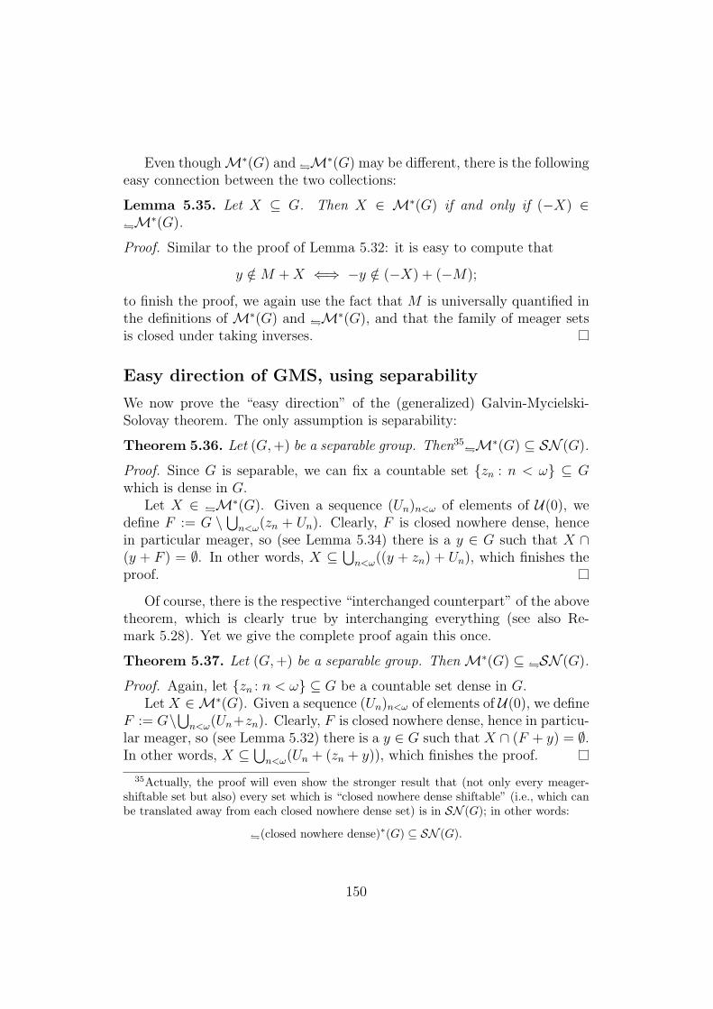
Even thoughM∗(G) and �M∗(G) may be different, there is the followingeasy connection between the two collections:

Lemma 5.35. Let X ⊆ G. Then X ∈ M∗(G) if and only if (−X) ∈�M∗(G).

Proof. Similar to the proof of Lemma 5.32: it is easy to compute that

y /∈M +X ⇐⇒ −y /∈ (−X) + (−M);

to finish the proof, we again use the fact that M is universally quantified inthe definitions of M∗(G) and �M∗(G), and that the family of meager setsis closed under taking inverses.

Easy direction of GMS, using separability

We now prove the “easy direction” of the (generalized) Galvin-Mycielski-Solovay theorem. The only assumption is separability:

Theorem 5.36. Let (G,+) be a separable group. Then35�M∗(G) ⊆ SN (G).

Proof. Since G is separable, we can fix a countable set {zn : n < ω} ⊆ Gwhich is dense in G.

Let X ∈ �M∗(G). Given a sequence (Un)n<ω of elements of U(0), wedefine F := G \

⋃n<ω(zn + Un). Clearly, F is closed nowhere dense, hence

in particular meager, so (see Lemma 5.34) there is a y ∈ G such that X ∩(y + F ) = ∅. In other words, X ⊆

⋃n<ω((y + zn) + Un), which finishes the

proof.

Of course, there is the respective “interchanged counterpart” of the abovetheorem, which is clearly true by interchanging everything (see also Re-mark 5.28). Yet we give the complete proof again this once.

Theorem 5.37. Let (G,+) be a separable group. ThenM∗(G) ⊆ �SN (G).

Proof. Again, let {zn : n < ω} ⊆ G be a countable set dense in G.Let X ∈M∗(G). Given a sequence (Un)n<ω of elements of U(0), we define

F := G\⋃n<ω(Un+zn). Clearly, F is closed nowhere dense, hence in particu-

lar meager, so (see Lemma 5.32) there is a y ∈ G such that X ∩ (F + y) = ∅.In other words, X ⊆

⋃n<ω(Un + (zn + y)), which finishes the proof.

35Actually, the proof will even show the stronger result that (not only every meager-shiftable set but also) every set which is “closed nowhere dense shiftable” (i.e., which canbe translated away from each closed nowhere dense set) is in SN (G); in other words:

�(closed nowhere dense)∗(G) ⊆ SN (G).

150

However, it seems to be unclear whether one can showM∗(G) ⊆ SN (G)(or �M∗(G) ⊆ �SN (G)) without any further assumptions.

Difficult direction of GMS, using compactness

We first prove36 Theorem 5.38: it is the “core” of the proof, so to speak, andis sufficient to immediately yield a version of the Galvin-Mycielski-Solovaytheorem for compact groups.

We can then use it to derive even more general versions for certain classesof locally compact groups.

Theorem 5.38. Let (G,+) be a locally compact group, and fix a witness, i.e.,a neighborhood W ∈ U(0) of the identity with the property that its topologicalclosure W is compact.

Then for every X ∈ SN (G) with X ⊆ W , we have X ∈M∗(G).

Before we prove the theorem, we give the “difficult direction of the Galvin-Mycielski-Solovay theorem” for compact groups as a corollary:

Corollary 5.39. Let (G,+) be a compact group. Then

SN (G) ⊆M∗(G).

Proof. Let X ∈ SN (G). Since G is compact, we just let G =: W ∈ U(0) bethe “neighborhood” of the identity with compact closure W = W = G. SoX ⊆ W is a void assumption, and Theorem 5.38 yields X ∈M∗(G).

In particular, Corollary 5.39 applies to the Cantor space (2ω,+). This isthe second time we obtain the Galvin-Mycielski-Solovay theorem for 2ω asa special case of a more general theorem: Theorem 5.10 in Section 5.1 alsoyields SN (2ω) =M∗(2ω).

Proof of Theorem 5.38. First note that not only W itself, but also W + Whas compact closure (to see this, recall that W ×W ⊆ G×G is compact, soits image under the addition mapping + : G × G → G is compact as well,i.e., +[W × W ] = W + W ⊆ G is compact; therefore W +W is compactsince it is a closed subset of the compact set W +W ). Let

K := W +W

36This is the theorem (or actually rather Corollary 5.39) I proved independently ofMarcin Kysiak (by generalizing the “usual” Galvin-Mycielski-Solovay theorem for R etc.using Lebesgue’s covering lemma for groups) before I learned at the Winterschool 2013in Hejnice (Czech Republic) that Kysiak had already done the same for locally compactPolish groups (see [Kys00]). I thank Piotr Zakrzewski for pointing this out to me.

151

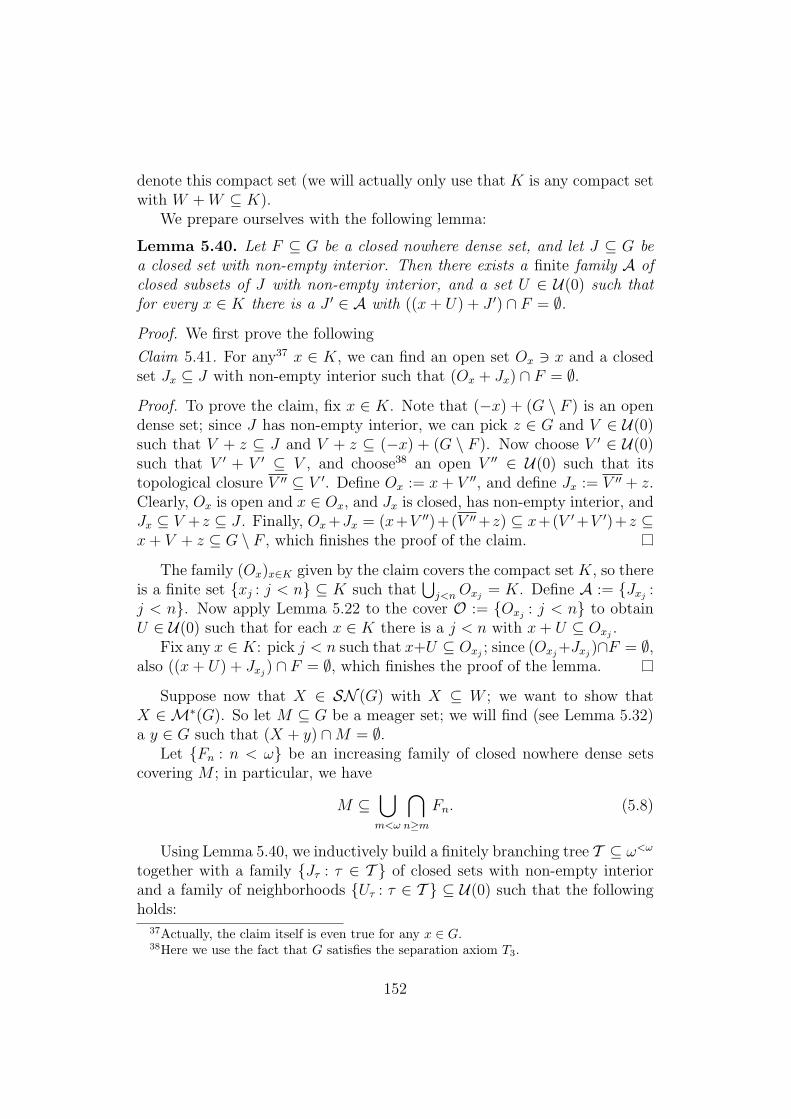
denote this compact set (we will actually only use that K is any compact setwith W +W ⊆ K).

We prepare ourselves with the following lemma:

Lemma 5.40. Let F ⊆ G be a closed nowhere dense set, and let J ⊆ G bea closed set with non-empty interior. Then there exists a finite family A ofclosed subsets of J with non-empty interior, and a set U ∈ U(0) such thatfor every x ∈ K there is a J ′ ∈ A with ((x+ U) + J ′) ∩ F = ∅.

Proof. We first prove the following

Claim 5.41. For any37 x ∈ K, we can find an open set Ox 3 x and a closedset Jx ⊆ J with non-empty interior such that (Ox + Jx) ∩ F = ∅.

Proof. To prove the claim, fix x ∈ K. Note that (−x) + (G \ F ) is an opendense set; since J has non-empty interior, we can pick z ∈ G and V ∈ U(0)such that V + z ⊆ J and V + z ⊆ (−x) + (G \ F ). Now choose V ′ ∈ U(0)such that V ′ + V ′ ⊆ V , and choose38 an open V ′′ ∈ U(0) such that itstopological closure V ′′ ⊆ V ′. Define Ox := x+ V ′′, and define Jx := V ′′ + z.Clearly, Ox is open and x ∈ Ox, and Jx is closed, has non-empty interior, andJx ⊆ V +z ⊆ J . Finally, Ox+Jx = (x+V ′′)+(V ′′+z) ⊆ x+(V ′+V ′)+z ⊆x+ V + z ⊆ G \ F , which finishes the proof of the claim.

The family (Ox)x∈K given by the claim covers the compact set K, so thereis a finite set {xj : j < n} ⊆ K such that

⋃j<nOxj = K. Define A := {Jxj :

j < n}. Now apply Lemma 5.22 to the cover O := {Oxj : j < n} to obtainU ∈ U(0) such that for each x ∈ K there is a j < n with x+ U ⊆ Oxj .

Fix any x ∈ K: pick j < n such that x+U ⊆ Oxj ; since (Oxj+Jxj)∩F = ∅,also ((x+ U) + Jxj) ∩ F = ∅, which finishes the proof of the lemma.

Suppose now that X ∈ SN (G) with X ⊆ W ; we want to show thatX ∈ M∗(G). So let M ⊆ G be a meager set; we will find (see Lemma 5.32)a y ∈ G such that (X + y) ∩M = ∅.

Let {Fn : n < ω} be an increasing family of closed nowhere dense setscovering M ; in particular, we have

M ⊆⋃m<ω

⋂n≥m

Fn. (5.8)

Using Lemma 5.40, we inductively build a finitely branching tree T ⊆ ω<ω

together with a family {Jτ : τ ∈ T } of closed sets with non-empty interiorand a family of neighborhoods {Uτ : τ ∈ T } ⊆ U(0) such that the followingholds:

37Actually, the claim itself is even true for any x ∈ G.38Here we use the fact that G satisfies the separation axiom T3.

152

0. J〈〉 = K.39

1. For each τ0, τ1 ∈ T : whenever τ0 ⊆ τ1, then Jτ0 ⊇ Jτ1 .

2. For each τ ∈ T :

for every x ∈ K, there is an immediate successor τa〈j〉 ∈ T of τ suchthat40

((x+ Uτ ) + Jτa〈j〉) ∩ F|τ | = ∅. (5.9)

It is straightforward to construct such a tree and the corresponding families:just note that K is a compact (hence closed) set with non-empty interior, sowe can start with J〈〉 := K and apply Lemma 5.40 to it (and F0) to obtainU〈〉 and the finite set A =: {J〈j〉 : j < |A|} satisfying the required properties;then continue by induction, repeatedly applying Lemma 5.40.

Note that the tree T is finitely branching (hence each level is finite), sowe can define for each n < ω

Un := (−W ) ∩⋂

τ∈T ∩ωnUτ ∈ U(0). (5.10)

Since X ∈ SN (G), we can (see Lemma 5.26) fix a sequence (xn)n<ω ofelements of X such that

X ⊆⋂m<ω

⋃n≥m

(xn + Un). (5.11)

Clearly, we can assume without loss of generality that (xn + Un) ∩ X 6= ∅for all n ∈ ω: otherwise, some of the (xn + Un) would not contribute to theunion anyway (so we could just omit them, or change the respective xn’sto “artificially make them contribute”). Consequently, we can assume thateach xn belongs to our compact set K: recall that Un ⊆ (−W ) and X ⊆ W ;therefore, (xn +Un)∩X ⊆ (xn + (−W ))∩W 6= ∅, hence xn ∈ W +W ⊆ K.

By induction, we construct a branch b through T (i.e., b ∈ [T ]) such thatfor each n < ω, we have

((xn + Un) + Jb�(n+1)) ∩ Fn = ∅; (5.12)

to do so, we just apply (in step n) property (2) of the tree T for τ := b�nto xn ∈ K to obtain b�(n + 1) satisfying (5.9), which yields (5.12) due toUn ⊆ Uτ (see (5.10)).

39Note that we can actually prove (X + y) ∩M = ∅ for “densely many” translationelements y, by letting J〈〉 be any small closed subset of K with non-empty interior insteadof K itself (see also (5.13)).

40Note that |τ | is the length of τ , i.e., at level n of the tree, we deal with the closednowhere dense set Fn.

153

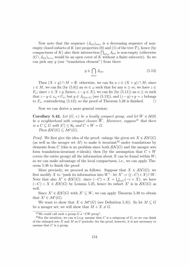
Now note that the sequence (Jb�n)n∈ω is a decreasing sequence of non-empty closed subsets of K (see properties (0) and (1) of the tree T ), hence (bycompactness of K) also their intersection

⋂n∈ω Jb�n is non-empty (otherwise

(G \ Jb�n)n<ω would be an open cover of K without a finite subcover). So wecan pick any y (our “translation element”) from there:

y ∈⋂n∈ω

Jb�n. (5.13)

Then (X + y) ∩M = ∅: otherwise, we can fix a z ∈ (X + y) ∩M ; sincez ∈M , we can fix (by (5.8)) an m ∈ ω such that for any n ≥ m, we have z ∈Fn; since z ∈ X+y (hence, z−y ∈ X), we can fix (by (5.11)) an n ≥ m suchthat z−y ∈ xn+Un; but y ∈ Jb�(n+1) (see (5.13)), and (z−y)+y = z belongsto Fn, contradicting (5.12); so the proof of Theorem 5.38 is finished.

Now we can derive a more general version:

Corollary 5.42. Let (G,+) be a locally compact group, and let W ∈ U(0)be a neighborhood with compact closure W . Moreover, suppose41 that thereis a C ⊆ G with |C| ≤ ℵ0 and C +W = G.

Then SN (G) ⊆M∗(G).

Proof. We first give the idea of the proof: enlarge the given set X ∈ SN (G)(as well as the meager set M) to make it invariant42 under translations byelements from C (this is no problem since both SN (G) and the meager setsform translation-invariant σ-ideals); then (by the assumption that C + Wcovers the entire group) all the information about X can be found within W ;so we can make advantage of the local compactness, i.e., we can apply The-orem 5.38 to finish the proof.

More precisely, we proceed as follows. Suppose that X ∈ SN (G); wefirst modify X to “push its information into W”: let X ′ := ((−C) +X)∩W .Note that also X ′ ∈ SN (G): since (−C) + X =

⋃c∈C(−c + X), we have

(−C) + X ∈ SN (G) by Lemma 5.25, hence its subset X ′ is in SN (G) aswell.

Since X ′ ∈ SN (G) with X ′ ⊆ W , we can apply Theorem 5.38 to obtainthat X ′ ∈M∗(G).

We want to show that X ∈ M∗(G) (see Definition 5.31). So let M ⊆ Gbe a meager set; we will show that M +X 6= G.

41We could call such a group G a “CW group”.42For the intuition, we can w.l.o.g. assume that C is a subgroup of G, so we can think

of the enlarged sets X and M as C-periodic; for the proof, however, it is not necessary toassume that C is a group.

154

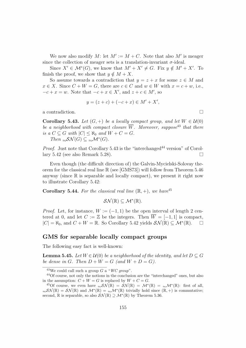
We now also modify M : let M ′ := M + C. Note that also M ′ is meagersince the collection of meager sets is a translation-invariant σ-ideal.

Since X ′ ∈ M∗(G), we know that M ′ + X ′ 6= G. Fix y /∈ M ′ + X ′. Tofinish the proof, we show that y /∈M +X.

So assume towards a contradiction that y = z + x for some z ∈ M andx ∈ X. Since C +W = G, there are c ∈ C and w ∈ W with x = c+ w, i.e.,−c+ x = w. Note that −c+ x ∈ X ′, and z + c ∈M ′, so

y = (z + c) + (−c+ x) ∈M ′ +X ′,

a contradiction.

Corollary 5.43. Let (G,+) be a locally compact group, and let W ∈ U(0)be a neighborhood with compact closure W . Moreover, suppose43 that thereis a C ⊆ G with |C| ≤ ℵ0 and W + C = G.

Then �SN (G) ⊆ �M∗(G).

Proof. Just note that Corollary 5.43 is the “interchanged44 version” of Corol-lary 5.42 (see also Remark 5.28).

Even though (the difficult direction of) the Galvin-Mycielski-Solovay the-orem for the classical real line R (see [GMS73]) will follow from Theorem 5.46anyway (since R is separable and locally compact), we present it right nowto illustrate Corollary 5.42:

Corollary 5.44. For the classical real line (R,+), we have45

SN (R) ⊆M∗(R).

Proof. Let, for instance, W := (−1, 1) be the open interval of length 2 cen-tered at 0, and let C := Z be the integers. Then W = [−1, 1] is compact,|C| = ℵ0, and C +W = R. So Corollary 5.42 yields SN (R) ⊆M∗(R).

GMS for separable locally compact groups

The following easy fact is well-known:

Lemma 5.45. Let W ∈ U(0) be a neighborhood of the identity, and let D ⊆ Gbe dense in G. Then D +W = G (and W +D = G).

43We could call such a group G a “WC group”.44Of course, not only the notions in the conclusion are the “interchanged” ones, but also

in the assumption: C +W = G is replaced by W + C = G.45Of course, we even have �SN (R) = SN (R) = M∗(R) = �M∗(R): first of all,

�SN (R) = SN (R) and M∗(R) = �M∗(R) trivially hold since (R,+) is commutative;second, R is separable, so also SN (R) ⊇M∗(R) by Theorem 5.36.

155

Proof. Let V ∈ U(0) such that (−V ) ⊆ W .To show that D + W = G, let x ∈ G be arbitrary. Since D is dense, we

can fix d ∈ D with d ∈ x+V . So, x ∈ d+ (−V ) ⊆ d+W , hence x ∈ D+W .The proof that W +D = G is analogous.

We can now conclude the main theorem of Section 5.2. Note that we donot assume that (G,+) is abelian.

Theorem 5.46. Let (G,+) be a separable, locally compact group. Then

�SN (G) = SN (G) =M∗(G) = �M∗(G).

Proof. Since G is locally compact, we can fix a neighborhood W ∈ U(0) suchthat its closure W is compact. Since G is separable, we can fix a dense setC ⊆ G with |C| ≤ ℵ0.

By Lemma 5.45, we know that C +W = G; so we can use Corollary 5.42to conclude

SN (G) ⊆M∗(G).

Again due to the separability of G, we can use Theorem 5.37 to obtain

M∗(G) ⊆ �SN (G).

Analogously, Corollary 5.43 yields (using W +C = G, again by Lemma 5.45)

�SN (G) ⊆ �M∗(G); lastly, Theorem 5.36 yields �M∗(G) ⊆ SN (G), fin-ishing the proof of the theorem.

Remark 5.47. In case of separable groups (e.g., R, or other locally com-pact – but non-compact – Polish groups such as Rn, etc.), it is typically an“overkill” to use a dense set C in the assumption of Corollary 5.42 to getC +W = G.

Indeed, a discrete set C may be enough for this purpose, as in the proofof Corollary 5.44, where C = Z ⊆ R. In that proof, we could have evenchosen W to be the half-open46 interval [−1

2, 1

2) of length 1; this would turn

our covering⋃z∈Z z + W into a “tiling” of R, i.e., each element x ∈ R is

represented in a unique way as x = z + w with z ∈ Z and w ∈ W .In my opinion, this illustrates (even though we need separability for the

easy direction of the Galvin-Mycielski-Solovay theorem anyway, and it is easyto get a countable set C with C+W = G from separability47 via Lemma 5.45)that always using a dense set C rather hides the point of the idea how topass from the compact setting (i.e., Theorem 5.38) to, e.g., locally compactPolish groups.

46Note that W need not be an open neighborhood for the proofs of this section. . .47For a situation without separability, see also item (6) on page 159.

156

GMS for Polish groups

Theorem 5.46 particularly yields the Galvin-Mycielski-Solovay theorem forlocally compact Polish groups (which has already been proved in [Kys00,Twierdzenie 5.5 (Galvin-Mycielski-Solovay) on page 34]):

Corollary 5.48. Let (G,+) be a locally compact Polish group. Then thenotions of being strong measure zero and being meager-shiftable coincide:

�SN (G) = SN (G) =M∗(G) = �M∗(G).

Proof. Since Polish groups are separable, the assumptions of Theorem 5.46are satisfied.

Here it is no problem to just talk about “strong measure zero” and“meager-shiftable” without mentioning whether SN (G) or �SN (G) (andM∗(G) or �M∗(G), respectively) are meant because (in the context of The-orem 5.46) the respective two notions coincide anyway.

But we can say even more: for locally compact Polish groups, the notionof strong measure zero the way we use it in this section (i.e., being in SN (G)according to Definition 5.23, which is “officially” called Rothberger bounded,see also Remark 5.24) coincides with the usual notion of strong measure zeroin metric spaces (see Definition 1.6), regardless of the metric being used (seeLemma 1.8).

Examples and remarks

We go through several topological groups in order to illustrate Theorem 5.46(and Corollary 5.42, respectively), also mentioning some “borderline cases”,and we show limitations of these theorems.

1. Typical examples of groups to which Theorem 5.46 can be appliedinclude compact Polish groups such as the Cantor space (2ω,+) withbitwise addition modulo 2, and the unit interval [0, 1] with additionmodulo 1 (in other words, the one-dimensional circle S1 with rotationas the group operation), as well as locally compact (but not compact)Polish groups such as the classical real line (R,+) and the topologicalvector spaces48 (Rn,+) etc. (all in the scope of Corollary 5.48).

48Also here (see Remark 5.47), it is not necessary to use separability for the difficultdirection of the Galvin-Mycielski-Solovay theorem, but W being a unit (hyper)cube andC being the set Zn of integer lattice points is fine, again forming a “tiling” of Rn.

157

2. As a trivial (but weird) “instance” of Theorem 5.46, let us considerthe finite cyclic group (Z17,+) of integers with addition modulo 17(necessarily49 with the discrete topology): clearly, it is separable andcompact (since it is finite), so Theorem 5.46 yields

SN (Z17) =M∗(Z17).

Let us also check this “by hand”: obviously, every set is in SN (Z17),i.e., SN (Z17) = P(Z17); on the other hand, every singleton {z} (forz ∈ Z17) is open, hence not nowhere dense, and so only the empty set ∅is meager; therefore every set X ⊆ Z17 can be translated away fromeach meager set, i.e., M∗(Z17) = P(Z17), and everything is fine.

3. Similarly, let us consider the infinite cyclic group (Z,+) of integers withthe discrete topology: again, it is separable (just because it is count-able); it is not compact, but locally compact ({0} ∈ U(0) is compact);so Theorem 5.46 again yields SN (Z) = M∗(Z). As in (2), only theempty set is meager, so once more we actually have

SN (Z) =M∗(Z) = P(Z).

4. Let us now consider the group (Q,+) of rational numbers with theusual topology (i.e., the topology inherited from R). Again, each setis in SN (Q) (just because it is countable); however, each singleton{q} (for q ∈ Q) is clearly nowhere dense, hence the entire group Q ismeager ; therefore only the empty set ∅ can be “translated away” fromeach meager set, i.e.,

P(Q) = SN (Q) 6=M∗(Q) = {∅}.

So the (difficult50 direction of the) Galvin-Mycielski-Solovay theoremfor (Q,+) fails: this is because Q is not locally compact.

However, (Q,+) is clearly σ-compact. This shows that the assumptionsof Corollary 5.42 cannot be weakened to just requiring that a compactset51 W with C +W = G (for some countable C) exists.

49Recall that we assume T3 for all our groups.50The easy direction is satisfied; this is no surprise since Q is separable.51The point where the proofs of Theorem 5.38 and Corollary 5.42 would break down

seems to be the following: by C + W = G, we can “push all the information” of X intoW ; but to make the compactness argument of Theorem 5.38 work, we have to make surethat not just the relevant part of X itself belongs to a compact set, but all the centers(xn) involved in the covering of X (see (5.11) on page 153 and the paragraph thereafter)belong to a compact set K; therefore we have to assume that not just W , but W plussome neighborhood is still compact.

158

5. We say that a topological group (G,+) is an insect if there exists anuncountable set in SN (G) and SN (G) =M∗(G).

We claim that there are non-metrizable insects.

For a cardinal κ ≥ ω, let (2κ×,+) denote the group 2κ (with bitwiseaddition modulo 2) equipped with the usual product (i.e., Tychonoff)topology. (Note that for κ > ω, the topology of (2κ×,+) is different fromthe topology of the group (2κ,+) considered in Section 5.1.) By Ty-chonoff’s theorem, (2κ×,+) is compact for all κ. We claim that (2ω1

× ,+)is a non-metrizable insect (even in ZFC). First of all, it is clearly notfirst-countable, hence not metrizable. Moreover, it is well-known thatthe (Tychonoff) product of at most continuum many separable spacesis separable, so (since ω1 ≤ c) (2ω1

× ,+) is separable; hence we can useTheorem 5.46 to conclude that SN (2ω1

× ) =M∗(2ω1× ). Lastly, the set

{f ∈ 2ω1 : ∃! i < ω1 f(i) = 1}

is of size ℵ1 and in SN (2ω1× ): given a sequence of Un’s – we can view

them as basic clopen neighborhoods of 0 with finite “supports” (wherethe 0’s are fixed) – we let i∗ be the supremum of all these supports;now we save one of the Un’s for later use, and cover all those (countablymany) f ’s that have their 1 below i∗ by the remaining countably manyUn’s; all the ω1 many remaining f ’s have only 0’s up to i∗, so we cancover them with the single saved neighborhood.

This shows that Theorem 5.46 is indeed a proper generalization ofCorollary 5.48 (which is for locally compact Polish groups only): itprovides non-trivial information about non-metrizable groups.

6. As in (5) above, let (2κ×,+) be equipped with the product topology.All these groups are compact. To get locally compact, non-compactgroups, we can add one single Z component, i.e., consider the groups

(Z× 2κ×,+) (5.14)

with the product topology (where plus is the component-wise addition).

In case of κ = ω, we just have an instance of Corollary 5.48 for locallycompact Polish groups.

In case of ω < κ ≤ c, we have a separable locally compact group, sowe have to use the more general Theorem 5.46 to get SN (Z × 2κ×) =M∗(Z× 2κ×).

159

In case of κ ≥ c+, our group in (5.14) is not separable any more, sowe may not expect to get the easy inclusion of the Galvin-Mycielski-Solovay theorem. The difficult one, however, still holds by Corol-lary 5.42: but this time we even have to use a countable C whichis not dense to obtain SN (Z× 2κ×) ⊆M∗(Z× 2κ×) (just because thereis no dense C available; see also Remark 5.47); e.g., let C = Z × {0}and W = {0} × 2κ×.

7. The Baer-Specker group (Zω,+) (which we will investigate in Sec-tion 5.3) is a Polish group which is not locally compact. So none ofthe theorems of this Section 5.2 can be applied to obtain the difficultinclusion SN (Zω) ⊆ M∗(Zω). Indeed, the main result of Section 5.3(see Theorem 5.53) shows that the (difficult direction of the) Galvin-Mycielski-Solovay theorem (consistently) fails for (Zω,+).

Questions

Regarding the pairs (“interchanged versions”) of definitions for strong mea-sure zero sets (see Definitions 5.23 and 5.27) and meager-shiftable sets (seeDefinitions 5.31 and 5.33), there is the following natural problem:

Question 5.49. Are there (Polish) groups (G,+) for which

1. SN (G) 6= �SN (G), or

2. M∗(G) 6= �M∗(G).

Note that the only candidates are (Polish) groups that are neither abeliannor locally compact (see Theorem 5.46).

I believe that the group (S∞, ◦) of permutations of ω could be a goodcandidate to find sets distinguishing the respective collections.

5.3 Failure of GMS for Zω

In this section, we investigate the Baer-Specker group Zω. We show thatthe Galvin-Mycielski-Solovay theorem (consistently) fails for Zω (see Theo-rem 5.53). This answers a question I was asked by Marcin Kysiak during theWinterschool 2011 in Hejnice (Czech Republic). I would like to thank himfor asking me this question, and for many interesting conversations there.

160

The Baer-Specker group Zω

The Baer-Specker group is the topological group (Zω,+), where additionis defined component-wise, i.e., for x, y ∈ Zω, its sum x + y is given by(x+ y)(n) := x(n) + y(n) for each n < ω; furthermore, Zω is equipped withthe product topology; in other words, the topology is generated by the basicclopen sets [s] := {z ∈ Zω : z ⊇ s} (for s ∈ Z<ω).

Note that (Zω,+) is an abelian Polish group (in particular, it is separable).However, (Zω,+) is not locally compact : this is because a basic clopen set [s]can never be compact since its open cover ([san])n<ω (indeed, it is a partitionof [s]) obviously has no finite subcover.

SN (Zω) — the strong measure zero sets

Let ωω↑ denote the collection of strictly increasing functions in ωω.Note that a set X ⊆ Zω is strong measure zero (i.e., X ∈ SN (Zω) ac-

cording to Definition 5.23) if and only if for every strictly increasing functionf ∈ ωω↑, there exists a sequence (sn)n<ω in Z<ω with |sn| ≥ f(n) for all nsuch that X ⊆

⋃n<ω[sn].

Also note that whenever d is a (compatible) translation-invariant52 met-ric, the above notion of strong measure zero coincides with the notion ofstrong measure zero with respect to d (see Definition 1.6); however, the no-tion of strong measure zero in the metric sense is not independent of themetric in this case (after all, Lemma 1.8 does not apply since Zω is notlocally compact).

M∗(Zω) — the meager-shiftable sets

A set X ⊆ Zω is meager-shiftable (i.e., X ∈ M∗(Zω) according to Defini-tion 5.31) if and only if for every meager set M ⊆ Zω, there is a y ∈ Zω suchthat (X + y) ∩M = ∅ (see Lemma 5.32).

Easy relations between SN (Zω) and M∗(Zω)

The following inclusions are easy:

Lemma 5.50. In ZFC, we have [Zω]≤ℵ0 ⊆M∗(Zω) ⊆ SN (Zω).

Proof. The first inclusion follows from the fact that the collection of meagersets on Zω forms a proper translation-invariant σ-ideal (see also the paragraphafter Definition 5.31 on page 148).

52Since (Zω,+) is abelian, we need not talk about left- and right-invariant metrics.

161

The second inclusion is the “easy direction” of the Galvin-Mycielski-Solovay theorem: recall that Zω is separable (and abelian), and apply Theo-rem 5.36.

We are going to show that the (difficult direction of the) Galvin-Mycielski-Solovay theorem “fails” for Zω, i.e., SN (Zω) *M∗(Zω). However, we cannotexpect to get it in ZFC. The reason is the following:

Lemma 5.51. Suppose that the Borel Conjecture holds. Then

[Zω]≤ℵ0 =M∗(Zω) = SN (Zω).

Proof. Since BC holds, Theorem 1.7 implies SN (Zω) = [Zω]≤ℵ0 . Thereforeall three collections are the same (see Lemma 5.50).

So the “Galvin-Mycielski-Solovay characterization for strong measure zerosets” consistently holds in Zω (in a trivial way, though).

Remark 5.52. Alternatively, we can argue in an elementary way here.The assertions SN (2ω) = [2ω]≤ℵ0 (i.e., the “usual” BC) and the assertionSN (Zω) = [Zω]≤ℵ0 (i.e., “BC for Zω”) are trivially equivalent, for the follow-ing reason: for the direction from left to right (this is the one we actually needfor Lemma 5.51), note that each element of Zω can be canonically53 mappedto an element of 2ω (with infinitely many 1’s), hence each uncountable set inSN (Zω) can be “interpreted” as an uncountable set in 2ω which is in SN (2ω)because the diameters of basic clopen sets only become smaller under thismapping; for the other direction, note that 2ω can be (literally) viewed as asubset of Zω (i.e., the mapping is the “identity”), so the argument is evensimpler.

The main theorem: SN (Zω) *M∗(Zω) (under CH)

We now prove the main theorem of this section: the difficult direction of theGalvin-Mycielski-Solovay theorem consistently fails. We present the theo-rem under the assumption of CH, but actually less is sufficient to make thearguments work (see Remark 5.57).

Theorem 5.53. Assume CH. Then SN (Zω) *M∗(Zω).

This actually says (see Lemma 5.50) that the meager-shiftable sets form aproper subcollection of the strong measure zero sets, i.e.,M∗(Zω) $ SN (Zω).

53Think of the homeomorphism between 2ω \Q and ωω via counting (for an element of2ω \Q) the numbers of 0’s between two 1’s.

162

Proof of Theorem 5.53. For s ∈ Z<ω, let [s] denote the set {t ∈ Z<ω : t ⊇ s}(or {x ∈ Zω : x ⊇ s}, depending on the context); for s0, s1 ∈ Z<ω, let s0

as1

be their concatenation; let 0(k) = 〈0, . . . , 0〉 be the element of Z<ω consistingof k zeros; and let |s| denote the length of s. For a tree F ⊆ Z<ω, let [F ] ⊆ Zωbe the set of all branches through F .

Fix a function ι : ω → Z<ω such that {n ∈ ω : ι(n) = s} is infinite foreach s ∈ Z<ω. For g ∈ ωω↑, let

F g := Z<ω \⋃n∈ω

[ι(n)a〈2 g(n)〉a0(g(n))].

Note that [F g] ⊆ Zω is a closed nowhere dense set.Let m : Z<ω → ω be defined by m(s) := max({s(i) : i < |s|}∪{1}). Now

letF ∗ := Z<ω \

⋃s∈Z<ω

[sa0(m(s))].

Again, note that [F ∗] ⊆ Zω is a closed nowhere dense set.We need the following feature of F ∗:

Lemma 5.54. Let s ∈ Z<ω, and let k ∈ ω \ {0}. If s is in F ∗, then eacht ∈ Z<ω with t ⊇ sa〈k〉 and |t| ≤ |s|+ k is in F ∗ as well.

Proof. Let s ∈ F ∗ and k > 0; suppose t ⊇ sa〈k〉 and |t| ≤ |s| + k. Assume(towards contradiction) that t is not in F ∗. Then there is an s′ ∈ Z<ωsuch that t ⊇ s′a0(m(s′)); since t ⊇ sa〈k〉, either sa〈k〉 ⊆ s′a0(m(s′)) ors′a0(m(s′)) ⊆ sa〈k〉; in either case, we reach a contradiction: in the first case,sa〈k〉 ⊆ s′ (recall k 6= 0), hence (by definition of m) we have m(s′) ≥ k andtherefore |t| ≥ |s′|+ k ≥ |s|+ 1 + k; in the second case, s′a0(m(s′)) ⊆ s, hences /∈ F ∗.

For s ∈ Z<ω and y ∈ Zω, we will abbreviate s+ y�|s| by s� y. Note thats� y is in Z<ω (and |s� y| = |s|), not in Zω.

Lemma 5.55. Let y ∈ Zω, and let g ∈ ωω↑. If s ∈ Z<ω satisfies s� y ∈ F ∗,then we can find an extension t ) s such that t = ι(n)a〈2 g(n)〉a0(g(n)) forsome n ∈ ω and t� y ∈ F ∗.

Proof. Since {n ∈ ω : ι(n) = s} is infinite for any s, and g is strictlyincreasing, we can choose n ∈ ω such that ι(n) = s and g(n) < 2 g(n)+y(|s|).(Note that y(|s|) ∈ Z can be negative, so this is not vacuously true.)

Define t := ι(n)a〈2 g(n)〉a0(g(n)). Since ι(n) = s, we have t ) s. Itremains to show that t� y ∈ F ∗.

163

Let k := 2 g(n) + y(|s|). We have t � y ⊇ (s � y)a〈k〉. Note that k > 0and |t � y| = |t| = |s| + 1 + g(n) ≤ |s| + k = |s � y| + k. Since s � y ∈ F ∗,the previous lemma yields t� y ∈ F ∗.

Lemma 5.56. Let y ∈ Zω, and let {gi : i ∈ ω} ⊆ ωω↑ be a countable set ofstrictly increasing functions. Then there is an x ∈ Zω such that

1. x /∈⋃i∈ω[F gi ],

2. x+ y ∈ [F ∗].

Proof. By induction, we will construct a sequence s0 ( s1 ( s2 · · · ∈ Z<ω.The required x ∈ Zω will then be

⋃i∈ω si.

We start with s0 := 〈〉 ∈ Z<ω. Note that 〈〉 ∈ F ∗ (by definition of F ∗), sos0 � y = 〈〉 ∈ F ∗. Given si with si � y ∈ F ∗, we can find (by Lemma 5.55)an extension si+1 ) si such that si+1 = ι(n)a〈2 gi(n)〉a0(gi(n)) for some n ∈ ωand si+1 � y ∈ F ∗. Define x :=

⋃i∈ω si.

For i ∈ ω, we have x ⊇ si+1 = ι(n)a〈2 gi(n)〉a0(gi(n)) for some n ∈ ω,hence x /∈ [F gi ]. And since si � y ∈ F ∗ for each i ∈ ω, we have x+ y ∈ [F ∗],which finishes the proof of the lemma.

To finish the proof of the theorem, we will construct a set X ⊆ Zω whichbelongs to SN (Zω) but does not belong54 to M∗(Zω).

Assuming CH, we can fix enumerations (yα : α < ω1) of Zω and (gα : α <ω1) of ωω↑. For each α < ω1, we apply Lemma 5.56 to get an xα such thatxα /∈

⋃β<α[F gβ ] and xα + yα ∈ [F ∗]. Define X := {xα : α < ω1}. It remains

to show that X ∈ SN (Zω) but X /∈M∗(Zω).First note that X /∈ M∗(Zω). This is witnessed by the set [F ∗] ⊆ Zω

which is nowhere dense, hence in particular meager. It suffices to show thatfor each y ∈ Zω, we have (X + y) ∩ [F ∗] 6= ∅: fix y ∈ Zω; pick α < ω1 suchthat yα = y; then xα + yα ∈ (X + y) ∩ [F ∗].

To show that X ∈ SN (Zω), fix a function f ∈ ωω↑. We will find asequence (sn)n∈ω in Z<ω with |sn| ≥ f(n) for each n such that X ⊆

⋃n∈ω[sn].

We split f into two functions g, h ∈ ωω↑, more precisely, let g and h be definedby g(n) = f(2n) and h(n) = f(2n + 1). Fix α < ω1 such that gα = g; notethat for any β > α, we have xβ /∈ [F gα ] = [F g]; in other words, {xβ : α <β < ω1} ⊆

⋃n∈ω[ι(n)a〈2 g(n)〉a0(g(n))]. Let s2n := ι(n)a〈2 g(n)〉a0(g(n)); then

|s2n| ≥ f(2n). Moreover, choose s2n+1 such that |s2n+1| ≥ f(2n+ 1) and the

54Note that we actually show that X does not belong to (closed nowhere dense)∗(Zω)either (which is a potentially stronger result) since we provide a witness (namely [F ∗])which is even closed nowhere dense (not just meager); see also footnote 35 on page 150.

I do not know, however, whether (closed nowhere dense)∗(Zω) andM∗(Zω) coincide ornot.

164

countable set {xβ : β < α} is covered by⋃n∈ω[s2n+1]. Then X ⊆

⋃n∈ω[sn],

and the proof of Theorem 5.53 is finished.

Remark 5.57. It is quite easy to see that it is not necessary to assume“full CH” in Theorem 5.53. In fact, cov(M) = 2ℵ0 (i.e., MA(countable)) issufficient: in Lemma 5.56 (as well as within the final argument to show thatX ∈ SN (Zω)), one can use density arguments for Cohen forcing to replace“countable” by “less than continuum”; note that Lemma 5.55 tells us thatthe required sets in Cohen forcing are dense.

Under CH, the first inclusion of Lemma 5.50 is a proper inclusion as well:

Lemma 5.58. Assume CH. Then [Zω]≤ℵ0 $ M∗(Zω), i.e., there exists anuncountable set in M∗(Zω).

Proof. This is a special case of Lemma 1.17: the meager sets on Zω forma translation-invariant and inverse-invariant σ-ideal containing all singletons(and have a basis of Fσ sets), hence CH implies that

ℵ1 = cov(M) = cof(M) = 2ℵ0 ,

so the lemma applies and yields an ℵ1 sized set in M∗(Zω).

Remark 5.59. As in Theorem 5.53, the weaker assumption55 cov(M) = 2ℵ0

is sufficient: as in the proof above, it yields cov(M) = cof(M) = 2ℵ0 , andhence the existence of a set of size continuum in M∗(Zω).

Corollary 5.60. The following two statements are consistent with ZFC:

1. [Zω]≤ℵ0 =M∗(Zω) = SN (Zω),

2. [Zω]≤ℵ0 $M∗(Zω) $ SN (Zω).

Proof. The first statement holds under BC (by Lemma 5.51).The second statement holds under CH: the first inclusion is proper by

Lemma 5.58, and the second inclusion is proper by Theorem 5.53.

Questions

I do not know whether any of the (two) remaining options is consistentwith ZFC:

Question 5.61. Is either of the following statements consistent with ZFC:

55. . . or here even cov(M) = cof(M), yielding an uncountable set of size cov(M).

165

1. [Zω]≤ℵ0 =M∗(Zω) $ SN (Zω),

2. [Zω]≤ℵ0 $M∗(Zω) = SN (Zω).

Note that the first scenario above could be called weak BC for Zω (butwithout the actual BC): to obtain a such model one could try to iterativelykill all uncountable meager-shiftable sets while avoiding to get full BC, i.e.,it is imaginable that one would need a kind of “gentle” Laver forcing.

A model for the second scenario would be a model in which the Galvin-Mycielski-Solovay characterization for Zω holds in a non-trivial way, i.e.,unlike in (1) of Corollary 5.60 (somehow “accidentally”, without the usualreason “local compactness”).

Using the terminology of item (5) on page 159, Question 5.61 (2) askswhether Zω can be an insect in some model of ZFC.

I actually do not know the answer for any (non locally compact) Polishgroup:

Question 5.62. Is every Polish insect56 locally compact?

In other words: Is local compactness of a Polish group (G,+) the onlyimaginable reason for satisfying M∗(G) = SN (G) in a non-trivial way?

More basically, I also tried to generalize Theorem 5.53 to the group(Rω,+), but unfortunately it didn’t work in a straightforward way. I conjec-ture that it can be done, though:

Question 5.63. Is their an analogue of Theorem 5.53 for other non locallycompact Polish groups (such as (Rω,+) or the group (S∞, ◦) of permutationsof ω)?

Let us mention one more question (see also footnote 54 on page 164):

Question 5.64. Is it consistent57 that the two collections

(closed nowhere dense)∗(G) and M∗(G)

differ for any Polish group (G,+)?

56Let us say that a butterfly is a Polish insect that is not locally compact. So theexistence of a model with a butterfly would answer the question to the negative.

57Note that BC must fail in this case; furthermore, the group must not be locallycompact since the collection (closed nowhere dense)∗(G) is in betweenM∗(G) and SN (G).

166

Chapter 6

Sacks dense ideals andMarczewski Borel Conjecture

In this chapter, I consider the Marczewski Borel Conjecture (MBC), a variantof the Borel Conjecture. Motivated by the question whether MBC is consis-tent, I introduce the notion of “Sacks dense ideal”. Even though Con(MBC)remains unsettled, I present several results about Sacks dense ideals.

In Section 6.1, we recall the class s0 of Marczewski null sets, consider theclass s∗0 of s0-shiftable sets, and introduce the Marczewski Borel Conjecture(the assertion that there are no uncountable s0-shiftable sets).

In Section 6.2, we introduce the main concept of this chapter: the notionof “Sacks dense ideal”. We prove – under CH – that any s0-shiftable setbelongs to all Sacks dense ideals.

In Section 6.3, we consider continuum many Sacks dense ideals (Jf )f∈ωωin order to confine the class of s0-shiftable sets (under CH); we derive thats0-shiftable sets are “very small” (namely null-additive, in particular strongmeasure zero). Moreover, we show the existence of uncountable sets thatbelong to all Jf .

In Section 6.4, we confine the s0-shiftable sets even further by introducinganother Sacks dense ideal, the “Vitali” Sacks dense ideal E0.

In Section 6.5, we explore the intersection of arbitrary families (of var-ious sizes) of Sacks dense ideals. Among other results, we show that theintersection of ℵ1 many Sacks dense ideals always contains uncountable sets.

In Section 6.6, we present one of the main results of this chapter (seeTheorem 6.48) which yields an abundance of Sacks dense ideals (under CH).

In Section 6.7, we comment on the collection s∗∗0 .

I thank Thilo Weinert for suggesting to consider the Marczewski BorelConjecture and the question whether it is consistent.

168

6.1 The Marczewski ideal s0 and the

Marczewski Borel Conjecture

In this section, we introduce a new variant of the Borel Conjecture: wereplace the ideal M in the definition of BC (the ideal N in the definitionof dBC, respectively) by the Marczewski ideal s0. We obtain an assertionwhich we call the Marczewski Borel Conjecture (MBC).

s0 — the Marczewski null sets

Recall that a (non-empty) set P ⊆ 2ω is called perfect if it is closed and hasno isolated points (in other words: if it is the set [T ] of branches through aperfect tree T ⊆ 2<ω).

Definition 6.1. A set Z ⊆ 2ω is Marczewski null (Z ∈ s0) if for each perfectset P ⊆ 2ω there is a perfect subset Q ⊆ P with Q ∩ Z = ∅.

It is well-known that s0 is a translation-invariant σ-ideal: Actually, the σ-closure can be shown by constructing a fusion-sequence of perfect sets (similarto the proof that Sacks forcing satisfies Axiom A, the Sacks property, etc.).Clearly, no perfect set (hence no uncountable Borel or analytic set) is in s0.

Note that each Z of size less than the continuum belongs to s0:

Lemma 6.2. Let Z ⊆ 2ω be such that |Z| < 2ℵ0. Then Z ∈ s0.

Proof. Fix a perfect set P ⊆ 2ω; we have to find a perfect subset Q ⊆ P suchthat Q ∩ Z = ∅.

Split P into “perfectly many” (hence 2ℵ0 many) perfect sets (Pα)α<2ℵ0 .Then there is a β < 2ℵ0 such that the perfect set Q := Pβ ⊆ P is disjointfrom Z.

Moreover, s0 also contains “large” sets, i.e., sets of size continuum. Thisresult (as well as several related results) can be found in Miller’s survey article“Special Subset of the Real Line” (see [Mil84, Theorem 5.10]). We present1 aproof using a maximal almost disjoint family (“mad family”) of perfect sets(in forcing terminology: a maximal antichain in Sacks forcing):

Lemma 6.3. There exists a set Z ⊆ 2ω of size continuum with Z ∈ s0.

1I thank Thilo Weinert for coming up with this proof during the Young Set TheoryWorkshop 2009 in Barcelona.

169

Proof. A family (Pα : α < 2ℵ0) of perfect subsets of 2ω is almost disjointif for all α, β < 2ℵ0 , α 6= β implies |Pα ∩ Pβ| ≤ ℵ0. (Note that for twoperfect sets P,Q ⊆ 2ω, P ∩ Q is closed, hence either at most countable orof size continuum, therefore we have in general |P ∩ Q| ≤ ℵ0 if and only if|P ∩Q| < 2ℵ0 .)

Such a family is called maximal if for any perfect set P ⊆ 2ω, there is anα < 2ℵ0 such that |P ∩ Pα| > ℵ0.

Fix a maximal almost disjoint family (Pα : α < 2ℵ0) of perfect sets. Toobtain such a family, just start with any family of continuum many disjointperfect sets (e.g., partition 2ω into “perfectly many” perfect sets), and extendthis (almost disjoint) family to a maximal one (by Zorn’s lemma).

Now we construct Z = {zα : α < 2ℵ0} of size continuum as follows: forany α < 2ℵ0 , we pick zα /∈

⋃β<α Pβ ∪ {zβ : β < α}; this is always possible,

since |Pα ∩ Pβ| = ℵ0 for every β < α, hence |Pα ∩⋃β<α Pβ| < 2ℵ0 , i.e.,

Pα \ (⋃β<α Pβ ∪ {zβ : β < α}) 6= ∅ (so we can actually pick zα ∈ Pα if we

wish). Clearly, |Z| = 2ℵ0 .It remains to show that Z ∈ s0. Fix a perfect set P ⊆ 2ω; we have to

find a perfect subset Q ⊆ P such that Q ∩ Z = ∅. By the maximality of ourfamily (Pα : α < 2ℵ0), we can fix β < 2ℵ0 such that |P ∩ Pβ| > ℵ0. SinceP ∩ Pβ is closed, there exists a perfect set Q′ ⊆ P ∩ Pβ. By construction,we have zα /∈ Pβ ⊇ Q′ for any α > β, i.e., Q′ ∩ Z ⊆ {zγ : γ ≤ β}. But|{zγ : γ ≤ β}| < 2ℵ0 , so by Lemma 6.2, there exists a perfect set Q ⊆ Q′ suchthat Q ∩ {zγ : γ ≤ β} = ∅, i.e., we have found our perfect set Q ⊆ P withQ ∩ Z = ∅.

s∗0 — the s0-shiftable sets

Recall that (for Y, Z ⊆ 2ω and t ∈ 2ω) Y + Z := {y + z : y ∈ Y, z ∈ Z},and Y + t := {y + t : y ∈ Y }, where, given two elements y, z ∈ 2ω, itssum y + z is the “bitwise sum modulo 2”, i.e., y + z is the real satisfying(y + z)(n) = y(n) + z(n) mod 2 for each n < ω.

Note that y + z = z + y, and −y = y, so it is “very easy” to rearrangeequations etc.

Definition 6.4. A set Y ⊆ 2ω is s0-shiftable (Y ∈ s∗0) if for each set Z ∈ s0

we have Y + Z 6= 2ω.

Note that Y + Z 6= 2ω if and only if Y can be “translated away” from Z(i.e., there is a “translation real” t ∈ 2ω such that (Y + t) ∩ Z = ∅).

Since s0 is a translation-invariant σ-ideal, it is easy to see that the col-lection s∗0 is translation-invariant, and contains all countable sets of reals,

170

i.e.,[2ω]≤ℵ0 ⊆ s∗0. (6.1)

However, I think there is no reason to believe that the collection s∗0 alwaysforms a σ-ideal (compare with the case of null-shiftable – i.e., strongly meager– sets, where CH even prevents them from being an ideal; see [BS01]).

MBC — the Marczewski Borel Conjecture

Recall that the Borel Conjecture is the assertion that there are no un-countable strong measure zero sets; by the Galvin-Mycielski-Solovay theoremfor 2ω, we know that the meager-shiftable sets coincide with the strong mea-sure zero sets; by definition, the strongly meager sets are the null-shiftablesets; the dual Borel Conjecture is the assertion that there are no uncountablestrongly meager sets:

BC ⇐⇒ M∗ = SN = [2ω]≤ℵ0

dBC ⇐⇒ N ∗ = SM = [2ω]≤ℵ0

We introduce the respective variant of BC for the Marczewski ideal s0:

Definition 6.5. The Marczewski Borel Conjecture (MBC) is the assertionthat s∗0 = [2ω]≤ℵ0 .

In other words, MBC is the “s0-BC” (as BC is the M-BC, and dBC isthe N -BC).

What about the status of MBC (in models of ZFC)? In particular, I’minterested2 in the following question:

Question 6.6. Is MBC consistent with ZFC?

Actually, it is not too difficult to see that the negation of MBC is con-sistent. Indeed, cov(s0) > ℵ1 implies that all sets of size ℵ1 are in s∗0 (henceMBC fails): the Marczewski ideal s0 is translation-invariant, so given any Ywith |Y | = ℵ1 and any Z ∈ s0, the sum Y + Z =

⋃y∈Y y + Z is the union of

only ℵ1 many sets in s0, hence Y + Z 6= 2ω.But cov(s0) = ℵ2 = 2ℵ0 holds true in the Sacks model (the model obtained

by a countable support iteration of Sacks forcing S of length ω2): intuitively

2I thank Thilo Weinert for asking me this question during the Young Set Theory Work-shop 2009 in Barcelona, and for many fruitful conversations about this topic. Actually,my investigations presented in this chapter only originated because he wondered what isgoing to happen when M (or N ) in the definition of (d)BC is replaced by s0.

171

speaking, this is because Sacks reals tend to avoid sets in s0 since beingdisjoint from such sets is a dense property in Sacks forcing (by definition ofs0); since those “dense sets” are not really in the respective ground model,one has to refine the argument; for the details, see [JMS92, Theorem 1.2].

On the other hand, I do not know whether MBC is consistent. To in-vestigate this question, I introduced the concept of “Sacks dense ideal” (seeDefinition 6.9), and established a connection between s∗0 and Sacks denseideals (see Lemma 6.10). However, this connection only holds under CH.This was the incentive to study Sacks dense ideals – mainly in the contextof CH. Even though the question whether MBC is consistent (with CH) re-mains unsettled, I consider Sacks dense ideals interesting for their own sake;so they will be the main focus of the chapter.

Remark 6.7. One may ask why MBC does not obviously fail under CH, i.e.,why it is not straightforward to construct an uncountable set in s∗0 under CH.After all, it is rather easy to derive the failure of BC (or dBC, respectively)from CH: just perform a Luzin type construction of a strong measure zeroset, i.e., use the fact that there is a Borel basis (hence a basis of size ℵ1)of the σ-ideal of meager sets, etc.; alternatively, we can also use the generalLemma 1.17 to obtain uncountable sets inM∗ or N ∗; applying Lemma 1.17is no problem since CH implies that cov(M) = cof(M) = ℵ1 and cov(N ) =cof(N ) = ℵ1.

In contrast to the ideal M of meager sets and the ideal N of measurezero sets, the Marczewski ideal s0 does not have a basis consisting of Borelsets (since any uncountable Borel set contains a perfect set which definitelydoes not belong to s0). But even more is true: there is no basis of s0 of sizeless or equal the continuum, i.e., cof(s0) > 2ℵ0 ; this was noted by3 Fremlin;a slightly stronger result (namely cf(cof(s0)) > 2ℵ0) is shown in [JMS92,Theorem 1.3].

So we always have (also under CH) cov(s0) ≤ 2ℵ0 < cof(s0) which destroysthe hope for an easy construction of an uncountable s0-shiftable set with amethod similar to the one in Lemma 1.17.

6.2 Sacks dense ideals

In this section, we introduce the main concept of this chapter: the notion of“Sacks dense ideal”. We will investigate them in order to learn more aboutthe collection s∗0 (“towards MBC”, so to speak), but we are also interested in

3This is mentioned in the introduction of [JMS92] (right before Theorem 1.3 is listed).

172

them for their own sake. Note that many of the results require CH, in par-ticular, Lemma 6.10 below, which establishes the main connection betweens∗0 and Sacks dense ideals. Therefore we will often (but not always) restrict4

our attention to the CH case.

σ-ideals dense in Sacks forcing and “Sacks dense ideals”

Let us first introduce a weaker notion:

Definition 6.8. A collection J ⊆ P(2ω) is a σ-ideal dense in Sacks forcingif

1. J is a σ-ideal,

2. J contains all singletons (hence all countable sets),

3. J is “dense in Sacks forcing S”, i.e., each perfect set P contains aperfect subset Q ⊆ P which belongs to J .

However, we are mainly interested in the following stronger notion:

Definition 6.9. A collection J ⊆ P(2ω) is a Sacks dense ideal if

1. J is a σ-ideal,

2b. J is translation-invariant, i.e.,

∀Y ∈ J ∀t ∈ 2ω (Y ∈ J ⇐⇒ Y + t ∈ J ),

3. J is “dense in Sacks forcing S”, i.e., each perfect set P contains aperfect subset Q ⊆ P which belongs to J .

Note that a Sacks dense ideal contains all singletons; therefore the Sacksdense ideals are exactly the σ-ideals dense in Sacks forcing (according toDefinition 6.8) that are (in addition) translation-invariant.

To emphasize the difference to (not translation-invariant) σ-ideals densein Sacks forcing, we may sometimes say “translation-invariant Sacks denseideal” instead of just “Sacks dense ideal”.

4Whenever a theorem needs CH, we will explicitly say so.

173

Connecting s∗0 with Sacks dense ideals (under CH)

The following lemma is central to the investigation of s∗0 and was the incentivefor coming up with the notion of Sacks dense ideal in the first place:

Lemma 6.10. Assume CH. Let J be any Sacks dense ideal. Then s∗0 is asubset of J .

Proof. Let Y /∈ J . We have to prove that Y /∈ s∗0; for that purpose, we willconstruct a set Z ∈ s0 such that Y + Z = 2ω (i.e., “Z witnesses Y /∈ s∗0”).

As in Lemma 6.3, we fix a maximal almost disjoint family (Pα : α < 2ℵ0)of perfect sets, but this time “within our Sacks dense ideal J ”, i.e., with theadditional property that Pα ∈ J for any α < 2ℵ0 . To obtain such a family,we again start with any family of continuum many disjoint perfect sets, thenwe replace each perfect set of this family with a perfect subset which belongsto the ideal J (note that this is possible since J is “dense in Sacks forcing”),and then we extend it to a maximal5 almost disjoint family of perfect setsbelonging to J . (Note that such a family is automatically also maximal withrespect to any perfect set, i.e., for any perfect set P ⊆ 2ω, there is an α < 2ℵ0

with |P ∩ Pα| > ℵ0. This corresponds to the easy “forcing fact” that everyantichain which is maximal in a dense subforcing is also dense in the wholeforcing.)

Moreover, let us fix any enumeration (xα : α < 2ℵ0) of the reals, i.e.,2ω = {xα : α < 2ℵ0}.

We now inductively construct Z = {zα : α < 2ℵ0}. For any α < 2ℵ0 ,we pick zα ∈ (Y + xα) \

⋃β<α Pβ. This is always possible, for the following

reason: by assumption, Y /∈ J , so Y + xα /∈ J holds as well (since J istranslation-invariant); but all the Pβ belong to J , hence also

⋃β<α Pβ is

in J (since J is a σ-ideal6); therefore (Y + xα) \⋃β<α Pβ 6= ∅.

We claim that Z ∈ s0 and Y + Z = 2ω. The latter is obvious by con-struction: for any α < 2ℵ0 , xα ∈ Y +Z, since zα was chosen to be in Y + xα.

So it remains7 to show that Z ∈ s0. Fix a perfect set P ⊆ 2ω; we have tofind a perfect subset Q ⊆ P such that Q∩Z = ∅. Since J is “dense in Sacksforcing”, there is a perfect set P ′ ⊆ P with P ′ ∈ J . By the maximality of(Pα : α < 2ℵ0) within J , we can fix β < 2ℵ0 such that |P ′ ∩ Pβ| > ℵ0. SinceP ′ ∩ Pβ is closed, there exists a perfect set P ′′ ⊆ P ′ ∩ Pβ. By construction,we have zα /∈ Pβ ⊇ P ′′ for any α > β, i.e., P ′′ ∩ Z ⊆ {zγ : γ ≤ β}. But|{zγ : γ ≤ β}| < 2ℵ0 , so by Lemma 6.2, there exists a perfect set Q ⊆ P ′′

5I.e., for any perfect set P ∈ J , there is an α < 2ℵ0 with |P ∩ Pα| > ℵ0.6For the argument to go through in ZFC, we would have to assume add(J ) = 2ℵ0 here

(instead of just σ-ideal – under CH, it is the same anyway); see also Remark 6.11.7The rest of the argument is essentially the same as in Lemma 6.3.

174

such that Q ∩ {zγ : γ ≤ β} = ∅, i.e., we have found our perfect set Q ⊆ Pwith Q ∩ Z = ∅.

In other words, the lemma says: A set in s∗0 belongs to the intersectionof all Sacks dense ideals.

Remark 6.11. An analogue of Lemma 6.10 holds true in general (i.e., with-out assuming CH) provided that we require our Sacks dense ideal to haveadditivity continuum; in other words: ZFC proves that s∗0 is a subset of everySacks dense ideal J satisfying add(J ) = 2ℵ0 (see footnote 6 for the point inthe proof where it is used).

However, this doesn’t seem to help finding a model of MBC: if CH fails, aSacks dense ideal with large additivity contains all ℵ1 sized sets, and so doestheir intersection; with this approach, we therefore cannot hope for excludingall uncountable sets from being in s∗0.

R — the intersection of all Sacks dense ideals

Let R denote8 the intersection of all Sacks dense ideals (we also refer to theelements of R as completely Sacks dense sets9 of reals):

Definition 6.12. R :=⋂{J : J is a Sacks dense ideal}.

Note that clearly R is a translation-invariant σ-ideal. With this notation,Lemma 6.10 says that s∗0 ⊆ R (under CH).

R and s~0

Under CH, we have s∗0 ⊆ R. We do not know whether the reverse inclusionR ⊆ s∗0 can be shown or not. However, it becomes true when replacing s∗0by s~0 .

In Chapter 1, we defined (for every I ⊆ P(2ω)) the collection I~ (seeDefinition 1.18 on page 22 and the discussion there). Recall that the collec-tion s~0 is related to s∗0 in the same way as the collection N~ = VM of verymeager sets is related to the collection N ∗ = SM of strongly meager sets:a set Y is in s~0 , if for every set Z ∈ s0 there exists a partition of Y intocountably many pieces (Yn)n<ω such that Yn + Z 6= 2ω for each n.

8R stands for “Raach”, the place (near Vienna) where the Young Set Theory Workshop2010 took place. I came up with the notion of Sacks dense ideal (and Lemma 6.10) duringthis conference.

9In a model of CH, let us say that a squirrel is an uncountable set in R, i.e., anuncountable completely Sacks dense set of reals; see also Question 6.46.

175

Lemma 6.13. R ⊆ s~0 .

Proof. Let Y ∈ R. We have to show that Y ∈ s~0 . More explicitly, we haveto show that for every set Z ∈ s0 there exists a partition of Y into countablymany pieces (Yn)n<ω such that for all n ∈ ω, we have Yn + Z 6= 2ω.

So let’s fix Z ∈ s0. We define a related Sacks dense ideal JZ as follows:for every perfect set P ⊆ 2ω, let us fix a perfect subset Q(P ) ⊆ P such thatQ(P ) ∩ Z = ∅ (this is possible since Z ∈ s0); define JZ to be the σ-idealgenerated by all translates of the sets Q(P ), i.e., let

JZ := σ〈{Q(P ) + t : P ⊆ 2ω perfect, t ∈ 2ω}〉.

It is easy to see that JZ is a Sacks dense ideal.By assumption, Y ∈ R =

⋂{J : J is a Sacks dense ideal}, so in partic-

ular we have Y ∈ JZ , i.e., for some family (Pn)n<ω of perfect sets and somefamily (tn)n<ω of “translation reals”, we have Y ⊆

⋃n<ω(Q(Pn) + tn). To

finish the proof, it is enough to show that (Q(Pn) + tn) + Z 6= 2ω (for anyn < ω), or, more generally, that (Q(P ) + t) + Z 6= 2ω (for any perfect setP ⊆ 2ω and any real t ∈ 2ω). But this is obvious, since t /∈ (Q(P ) + t) + Zis equivalent to Q(P )∩Z = ∅ which is true by our choice of the Q(P )’s.

Remark 6.14. Note that we didn’t need CH for the proof of Lemma 6.13.However, the CH issue is somewhat hidden, in the following sense. As dis-cussed in Remark 6.11, in order to make s∗0 ⊆ R hold true in general, wewould have to adapt the definition of R: replace “σ-ideal” by “additivity con-tinuum” in the definition of Sacks dense ideal. With respect to this adapteddefinition of R, Lemma 6.13 (i.e., R ⊆ s~0 ) only stays true when we also adaptthe definition of s~0 accordingly (replace “there is a partition into countablemany pieces” by “there is a partition into less than continuum many pieces”).

Note that (6.1), Lemma 6.10, the fact that R is a σ-ideal, and Lemma 6.13together yield the following:

CH −→ [2ω]≤ℵ0 ⊆ s∗0 ⊆ σ〈s∗0〉 ⊆ R ⊆ s~0 . (6.2)

Remark 6.15. In my opinion, (6.2) makes the connection between s∗0 andR (given by Lemma 6.10) even “tighter”, and hence more interesting.

Let me explain in more detail what I actually mean. I do not knowwhether MBC(+CH) is consistent, but in any model of MBC+CH, we wouldobviously have [2ω]≤ℵ0 = s∗0 = σ〈s∗0〉, so either [2ω]≤ℵ0 = R holds thereas well, or we would have [2ω]≤ℵ0 = σ〈s∗0〉 $ s~0 . If the latter holds, wewould have found the “remarkable example” of an ideal I (namely I = s0)with the property that σ〈I∗〉 6= I~. It seems to be unknown, whether this

176

situation is consistent for10 I = N , i.e., whether it is consistent that the σ-ideal generated by the strongly meager sets differs from the collection of verymeager sets (see Definition 1.20 on page 23 and the subsequent discussion).In the model of BC+dBC of our joint paper [GKSW] (see Chapter 2), thisis not the case, i.e., σ〈N ∗〉 = N~ holds there (see Theorem 3.1; actually, thewhole Chapter 3 is devoted to the proof of it).

By the above, MBC (i.e., s∗0 = [2ω]≤ℵ0) and R = [2ω]≤ℵ0 are “almostequivalent” — in the sense that any counterexample would yield σ〈s∗0〉 $ s~0 ,i.e., the above “remarkable case”.

Finding Sacks dense ideals “towards MBC”

Recall that my original incentive for studying Sacks dense ideals (and thecollection R) was the question whether the Marczewski Borel ConjectureMBC (i.e., the statement [2ω]≤ℵ0 = s∗0) is consistent or not. Since Lemma 6.10tells us how to confine s∗0 by Sacks dense ideals (but only under CH), thequestion (”towards MBC”) is whether we can – under CH – find “many Sacksdense ideals” (at least consistently).

It is straightforward to check that the ideal M of meager sets as well asthe ideal N of measure zero sets forms a Sacks dense ideal (and the σ-ideal Egenerated by the closed measure zero sets too), whereas for instance the idealSN of strong measure zero sets does not. Nevertheless (as we will show inthe next section) the strong measure zero sets can be “approximated fromabove” (by Sacks dense ideals), meaning that each set in the intersection R

of all Sacks dense ideals (and hence each set in s∗0) is strong measure zero.For now, let us just summarize what we have seen so far:

CH −→ [2ω]≤ℵ0 ⊆ s∗0 ⊆ R ⊆ E ⊆M∩N .

6.3 Confining s∗0 by Sacks dense ideals (Jf)f∈ωωIn this section, we investigate continuum many Sacks dense ideals Jf , inorder to confine the class s∗0 (under CH). Moreover, we show that sets ofreals that belong to all of the Jf ’s (and hence – under CH – sets in s∗0) are“very small” (namely null-additive, i.e., particularly strong measure zero).We also construct (under CH) uncountable sets which belong to all Jf .

Let me remark that some of my theorems (in particular Lemma 6.27 andTheorem 6.28) are very reminiscent of the construction in the first section of

10It is not for I =M; see Theorem 1.21.

177

Tomek Bartoszynski’s paper11 “Remarks on small sets of reals” (see [Bar03]),even though I came up with the proofs completely independently.

Sacks dense ideal Jf generated by f-tiny sets

For X ⊆ 2ω and k ∈ ω, let X�k abbreviate {x�k : x ∈ X}. Note thatX�k ⊆ 2k.

Definition 6.16. Let12 f ∈ ωω.

• We say that a set X ⊆ 2ω is f -tiny if for almost all k ∈ ω, we have|X�f(k)| ≤ k.

• Let Jf be the σ-ideal generated by the f -tiny sets:

Jf := σ〈{X ⊆ 2ω : X is f -tiny}〉.

Remark 6.17. We could have defined f -tiny by demanding |X�f(k)| ≤ k“for all13 k > 0” instead of “for almost all k”. This wouldn’t make a bigdifference though, since the resulting σ-ideal Jf is the same for both versions.

Moreover, note that the (perfect kernel of the) closure of an f -tiny set Xis again f -tiny, therefore

Jf = σ〈{P ⊆ 2ω : P perfect, P is f -tiny}〉;

in other words, we can think of Jf as generated by the perfect f -tiny setsonly.

By definition, every Jf is a σ-ideal; even more holds:

Lemma 6.18. Let f ∈ ωω. Then Jf is a Sacks dense ideal.

Proof. To show that the σ-ideal Jf is translation-invariant it suffices to notethat being f -tiny is a translation-invariant property (which is obvious).

It is also easy to see that Jf is dense in Sacks forcing. Fix a perfect setP ⊆ 2ω; we can think of it as a perfect tree, i.e., let T ⊆ 2<ω be the (unique)perfect tree such that P = [T ] (where [T ] is the set of branches through T ).Recall that t ∈ T is a splitting node if both ta0 and ta1 are in T . We thin

11I thank Tomasz Weiss for pointing out this paper to me during the conference “Trendsin set theory” in Warsaw 2012. I gave a talk there presenting part of the material of thischapter (including Theorem 6.48 which I had proved very shortly before the conference).

12We can w.l.o.g. assume that f is an increasing function.13Note that restricting it to k > 0 is necessary because |X�f(0)| ≤ 0 only holds for the

empty set X = ∅ ;-(

178

out the tree by removing14 sufficiently many splitting nodes. In this way, itis not difficult to obtain a “sufficiently thin” perfect subtree T ′ ⊆ T suchthat Q := [T ′] is f -tiny; in particular, the perfect set Q ⊆ P is in Jf .

Definition 6.19. We say that X is completely tiny if X belongs to all Jf ’s,i.e.,

X ∈⋂f∈ωωJf .

Note that Lemma 6.18 and Lemma 6.10 imply that (under CH) everys0-shiftable set is completely tiny:

CH −→ s∗0 ⊆⋂f∈ωωJf . (6.3)

We will show that a completely tiny set is “quite small” (see Theo-rem 6.28). Let us first outline the idea of why a completely tiny set is strongmeasure zero15 (which will follow from Theorem 6.28 anyway), i.e.,⋂

f∈ωωJf ⊆ SN . (6.4)

Fix X ∈⋂f∈ωω Jf , and let16 (kn)n<ω be an increasing fast-growing se-

quence of natural numbers; we can “translate” this sequence to an even fastergrowing17 function g ∈ ωω; since X ∈ Jg, the set X can be covered by count-ably many (perfect) sets that are g-tiny; each of these sets can be covered by“few” basic clopen sets [si] with |si| “large”; so if g was chosen appropriately,X can be covered by

⋃n[sn] with |sn| ≥ kn for each n < ω. This shows that

X is strong measure zero.

Remark 6.20. It may be tempting to try to derive Con(MBC) from (6.3)and (6.4) by considering a model of BC. However, this doesn’t work18 sinceBC requires 2ℵ0 > ℵ1, whereas (6.3) only holds under CH.

14“To remove a splitting node t” is supposed to mean “to keep either ta0 or ta1 withinthe tree, but to remove the other node (and each node extending it) from the tree”.

15Similarly, one can easily show that each completely tiny set is perfectly meager (whichalso follows from Theorem 6.28).

16This is – so to speak – the “εn-sequence” of the “elementary definition” of strongmeasure zero; see Definition 1.5.

17E.g., choose g such that g(1) ≥ k1, g(2) ≥ k1+2, g(3) ≥ k1+2+3, etc.; such a g shouldwork. . .

18An analogous remark applies to dBC and the fact that s∗0 ⊆ SM under CH (seeCorollary 6.30).

179

Fast-increasing towers are completely tiny

We now show (under CH) the existence of uncountable sets (namely “fast-increasing towers”) that are completely tiny, i.e., in

⋂f∈ωω Jf ; so let us recall

the concept of a (fast-increasing) tower.For each x ∈ 2ω, we identify x with the set {n : x(n) = 1} ⊆ ω (i.e., x is

the characteristic function of this set). Let Q := {z ∈ 2ω : ∀∞n (z(n) = 0)}denote the “rationals” of 2ω. If x ∈ 2ω \ Q, i.e., x is (the characteristicfunction of) an infinite subset of ω, we let enum(x) ∈ ωω be its enumeratingfunction, i.e., we let enum(x) be the unique strictly increasing function fsuch that its range {f(k) : k < ω} equals {n < ω : x(n) = 1}.

For two functions f, g ∈ ωω, let f ≤ g denote “f(n) ≤ g(n) for all n < ω”,and let f ≤∗ g denote “f(n) ≤ g(n) for almost all n < ω”. As usual, wesay that a subfamily of ωω is a dominating family if it is cofinal in ωω withrespect to ≤∗; the dominating number d is the smallest size of a dominatingfamily.

We are going to use the same notation for reals x, y ∈ 2ω ⊆ ωω, i.e., forreals x, y ∈ 2ω, let x ≤∗ y denote “x(n) ≤ y(n) for almost all n < ω”. Notethat x ≤∗ y if and only if x ⊆∗ y when x and y are viewed as subsets of ω(where ⊆∗ denotes almost inclusion, i.e., x ⊆∗ y means |x \ y| < ℵ0), andx ≤ y if and only if x ⊆ y.

Definition 6.21. A set X ⊆ 2ω \Q is a tower of length γ ≤ 2ℵ0 if

X = {xα : α < γ},

and for each α ≤ β < γ, we have xβ ≤∗ xα.A tower X = {xα : α < γ} ⊆ 2ω \Q of length γ is a fast-increasing tower

if the set {enum(xα) : α < γ} ⊆ ωω of its enumerating functions forms adominating family, i.e.,

∀g ∈ ωω ∃α < γ (g ≤∗ enum(xα)).

We now show that under certain circumstances concerning cardinal char-acteristics (in particular under CH), it is easy to construct a fast-increasingtower.

The tower number t is the smallest γ such that there exists a tower {xα :α < γ} of length γ without a pseudointersection, i.e., without any y ∈ 2ω \Qwith y ≤∗ xα for each α < γ. It is well-known that ℵ1 ≤ t ≤ d ≤ 2ℵ0 .

Lemma 6.22. Let t = d. Then there is a fast-increasing tower (of length d).

180

Proof. Let {gα : α < d} ⊆ ωω be a dominating family, i.e., for each g ∈ ωω,there is an α < d such that g ≤∗ gα. We will construct a fast-increasingtower X = {xα : α < d} ⊆ 2ω \Q of length d.

We construct the sequence (xα)α<d by induction. We start with anyx0 ∈ 2ω \Q such that g0 ≤ enum(x0). Given xα, we let xα+1 ∈ 2ω \Q be suchthat xα+1 ≤ xα and gα+1 ≤ enum(xα+1). At limits α, we use the fact thatα < t = d: given {xβ : β < α}, we can therefore find a pseudointersectiony ∈ 2ω \Q such that y ≤∗ xβ for every β < α; then, we again let xα ∈ 2ω \Qbe such that xα ≤ y and gα ≤ enum(xα) (in particular, we have xα ≤∗ xβ forevery β < α).

So X = {xα : α < d} is a tower. It is also fast-increasing: by construction,gα ≤ enum(xα) for every α < d; now fix any g ∈ ωω; then there is α < d suchthat g ≤∗ gα, hence g ≤∗ enum(xα).

In particular, CH implies the existence of a fast-increasing tower (of lengthω1 = 2ℵ0).

Lemma 6.23. Let X ⊆ 2ω be a fast-increasing tower of length ω1. Then Xis completely tiny, i.e., X ∈

⋂f∈ωω Jf .

Proof. Suppose that X = {xα : α < ω1} is a fast-increasing tower. We haveto prove that X is completely tiny. So fix19 an f ∈ ωω; we will show thatX ∈ Jf .

Let g ∈ ωω be defined by g(n) := f(2n+1) for each n < ω. By thefact that {xα : α < ω1} is fast-increasing, we can fix an α < ω1 such thatg ≤∗ enum(xα).

We first claim that the set Y := {y ∈ 2ω : y ≤ xα} (i.e., the “set of allsubsets of xα”) is f -tiny. Let enum(xα) =: h ∈ ωω. Since g ≤∗ h, we canfix N ∈ ω such that g(n) ≤ h(n) for each n ≥ N . We will show that foreach k ≥ 2N , we have |Y �f(k)| ≤ k. So fix k ≥ 2N . Let n < ω be such thatk ∈ [2n, 2n+1). Note that n ≥ N , so g(n) ≤ h(n) by our assumption on N .Moreover, we have f(k) < f(2n+1) = g(n) ≤ h(n). We have

|Y �f(k)| = |{s ∈ 2f(k) : s ≤ xα�f(k)}| = 2|xα∩f(k)|,

where xα ∩ f(k) actually denotes the set {j < f(k) : xα(j) = 1} (i.e., weview xα as a subset of ω here). But |xα ∩ f(k)| ≤ |xα ∩ h(n)| = n (sinceh = enum(xα) enumerates xα), therefore |Y �f(k)| ≤ 2n ≤ k, finishing theproof of our claim that Y is f -tiny.

To show that X ∈ Jf , note that Jf is a σ-ideal containing all countablesets of reals (since every singleton trivially is f -tiny, hence in Jf ). SinceX = {xβ : β < α}∪{xβ : β ≥ α}, it is enough to show that {xβ : β ≥ α} ∈ Jf .

19We can assume w.l.o.g. that f is strictly increasing.

181

Recall that Q = {z ∈ 2ω : ∀∞j (z(j) = 0)} denotes the “rationals” of 2ω.Since X is a tower, xβ ≤∗ xα for each β ≥ α; in other words: for each β ≥ α,there exists a y ≤ xα (i.e., y ∈ Y ) and a q ∈ Q such that xβ = q + y, i.e.,

{xβ : β ≥ α} ⊆ Q+ Y =⋃q∈Q

(q + Y ) ∈ Jf

(because Y is f -tiny, hence in Jf , and Jf is a translation-invariant σ-ideal);so {xβ : β ≥ α} ∈ Jf , finishing the proof.

So we have uncountable completely tiny sets under CH:

Corollary 6.24. Under CH, there exists an uncountable set in⋂f∈ωω Jf .

Proof. CH implies ℵ1 = t = d = 2ℵ0 , hence Lemma 6.22 yields the exis-tence of a fast-increasing tower X of length ω1. So by Lemma 6.23, X is in⋂f∈ωω Jf . Note that X is uncountable (since it is a dominating family).

Remark 6.25. We comment on another family of Sacks dense ideals (as analternative to (Jf )f∈ωω).

Recall that we can think of a perfect set P ⊆ 2ω as a perfect tree T ⊆ 2<ω

(with P = [T ]). Further recall that t ∈ T is a splitting node (t ∈ split(T ))if both ta0 and ta1 are in T . Let us say that the splitting nodes of T aremonotonously enumerated by g if g : ω → split(T ) is bijective and i < jimplies |g(i)| ≤ |g(j)|.

Let f ∈ ωω. Consider a tree T with the property that its splitting nodesare monotonously enumerated by some g with |g(i)| ≥ f(i) for (almost) everyi ∈ ω. Note that this more or less means that the perfect set [T ] is f -tiny.

We now define the following stronger notion: let us say that a perfecttree T (or the respective perfect set P = [T ]) is f -sparse if its splitting nodesare monotonously enumerated by some g with |g(i + 1)| − |g(i)| > f(i) forevery i ∈ ω. Let J sparse

f be the σ-ideal generated by the f -sparse perfect sets:

J sparsef := σ〈{P ⊆ 2ω : P is f -sparse}〉.

As in Lemma 6.18 for Jf , it is quite easy to check that J sparsef is a Sacks

dense ideal.Note that a function g with |g(i + 1)| − |g(i)| > f(i) (i.e., a witness for

being f -sparse) in particular satisfies that the mapping i 7→ |g(i)| is injective,therefore all trees with more than one splitting node at the same height areexcluded; especially, “uniform sets” such as the set Y = {y ∈ 2ω : y ≤ xα} inthe proof of Lemma 6.23 can never be f -sparse (but f -tiny for appropriate f).

182

Therefore it is not clear how to find (under CH) an uncountable set in⋂f∈ωω J

sparsef (by a tower construction, as in Corollary 6.24). However, the

much more general Theorem 6.41 below will indeed yield such an uncountableset (under CH).

Completely tiny sets are null-additive

We now prove that each completely tiny set (and hence – under CH – eachs0-shiftable set) is null-additive (hence strongly meager), and therefore (seeTheorem 6.29) also meager-additive, so in particular strong measure zero.

Recall the notion of I-additive for arbitrary I:

Definition 6.26. Let I ⊆ P(2ω). Define

I-additive := {X ⊆ 2ω : X + Z ∈ I for every set Z ∈ I}.

Clearly, I-additive ⊆ I∗ (provided 2ω /∈ I, which we always tacitly as-sume). In particular, each N -additive (i.e., null-additive) set is stronglymeager, and each M-additive (i.e., meager-additive) set is strong measurezero. Moreover, whenever I is a σ-ideal (translation-invariant), the collectionof I-additive sets is a σ-ideal (translation-invariant) as well.

Lemma 6.27. Given a measure zero set N ∈ N , we can find a functionf ∈ ωω such that for each X ⊆ 2ω,

X is f -tiny⇒ X +N ∈ N .

Proof. Fix N ∈ N . We find a function f ∈ ω as follows. It is easy to show(see, e.g., [Gol93, Fact 6.7(2)]) that there is a sequence of clopen sets (Cn)n<ωwith measure µ(Cn) ≤ 2−n for each n < ω such that N ⊆

⋂m<ω

⋃n≥mCn;

now each Cn is the union of finitely many basic clopen sets: for each n < ω,let ln < ω and sn,i ∈ 2<ω (for each i < ln) such that Cn =

⋃i<ln

[sn,i]; withoutloss of generality, we can assume that for each n < ω, all the (sn,i)i<ln are(distinct and) of the same length, and let f(n) be this common length; i.e.,let f ∈ ωω be such that f(n) = |sn,0| for each n < ω.20

We claim that this f works: so fix a set X which is f -tiny; we have toshow that X + N ∈ N . Since X is f -tiny, we can fix an N ∈ ω such that|X�f(n)| ≤ n for every n ≥ N .

20Note that µ(Cn) ≤ 2−n implies ln ≤ 2−n . 2f(n).

183

For the moment, fix n ≥ N . Note that21

X + Cn = X +⋃i<ln

[sn,i] = X�f(n) +⋃i<ln

[sn,i], (6.5)

hence “adding X to Cn” increases the measure of Cn by (at most) a factorof |X�f(n)| ≤ n, i.e.,22

µ(X + Cn) ≤ |X�f(n)| . µ(Cn) ≤ n . 2−n.

Now for each m < ω, N ⊆⋃n≥mCn, hence X + N ⊆

⋃n≥m(X + Cn).

Therefore, for each m ≥ N ,

µ(X +N) ≤∑n≥m

µ(X + Cn) ≤∑n≥m

n . 2−n −→ 0 (for m→∞),

so µ(X +N) = 0, i.e., X +N ∈ N .

Theorem 6.28. Every completely tiny set (i.e., every set in⋂f∈ωω Jf) is

N -additive.

Proof. Suppose that X is completely tiny, i.e., X ∈⋂g∈ωω Jg. We have to

prove that X is N -additive. So fix a null set N ∈ N ; we will show thatX +N ∈ N .

By Lemma 6.27, we can find a function f ∈ ωω such that Y + N ∈ Nwhenever Y ⊆ 2ω is f -tiny.

By assumption, X ∈ Jf (the σ-ideal generated by the f -tiny sets), i.e.,there are f -tiny sets (Xk)k<ω such that X ⊆

⋃k<ωXk. So Xk + N ∈ N for

each k < ω, hence

X +N ⊆⋃k<ω

(Xk +N) ∈ N

(using the fact that N is a σ-ideal), i.e., X +N ∈ N .

To derive that the set is small with respect to the other “notions ofsmallness” mentioned above, we use the following theorem of Shelah:

21Actually, X�f(n) is not a set of reals, but of elements of 2f(n) (of size at most n); sowhat we really mean with the right-most expression of (6.5) is the following: since thequestion whether a real belongs to

⋃i<ln

[sn,i] or not only depends on its restriction tof(n), it is sufficient to take any set of (at most n) “representative” reals for X�f(n) (itsrestrictions to f(n) belong to X�f(n)), yielding the same sum as X would yield.

22More formally: z ∈ X + Cn ↔ z�f(n) ∈ X�f(n) + {sn,i : i < ln} ⊆ 2f(n); but|X�f(n) + {sn,i : i < ln}| ≤ |X�f(n)| . |{sn,i : i < ln}| ≤ n . ln ≤ n . 2−n . 2f(n), henceµ(X + Cn) ≤ n . 2−n.

184

Theorem 6.29 (Shelah). Every N -additive set is M-additive.

Proof. See, e.g., [BJ95, Theorem 2.7.20], or the original paper [She95].

Let us summarize our results so far on “how small” s0-shiftable sets are:

Corollary 6.30. Assume CH. Then every s0-shiftable set is N -additive (andM-additive), so in particular both strong measure zero and strongly 23 mea-ger:

CH −→ s∗0 ⊆ SN ∩ SM.

Proof. By Lemma 6.10, Lemma 6.18, and Theorem 6.28,

s∗0 ⊆ R =⋂{J : J is a Sacks dense ideal} ⊆

⋂f∈ωωJf ⊆ N -additive.

Since N -additive ⊆ N ∗ = SM, each set in s∗0 is strongly meager.By Theorem 6.29, we have N -additive ⊆ M-additive ⊆ M∗ = SN , so

each set in s∗0 is strong measure zero.

6.4 Confining s∗0 even more: the Vitali Sacks

dense ideal E0

In this section, we introduce another Sacks dense ideal which we name E0

(derived from the “Vitali equivalence relation” on 2ω); we will prove (underCH) that being in the intersection of the Sacks dense ideals (Jf )f∈ωω is notenough for being in the intersection R of all Sacks dense ideals, i.e., E0

“contributes” to this intersection in a non-trivial way (see Corollary 6.35).In other words,

CH −→⋂f∈ωωJf % E0 ∩

⋂f∈ωωJf ⊇ R =

⋂{J : J is a Sacks dense ideal}.

Later (see Corollary 6.49) we will show (again under CH) that the secondinclusion is a proper inclusion as well.

23Hence also very meager (i.e., in VM; see Definition 1.20), and perfectly meager. Infact, the following holds (where PM denotes the collection of perfectly meager sets):

N -additive ⊆ N ∗ = SM ⊆ σ〈SM〉 ⊆ VM = N~ ⊆ PM ⊆M.

185

Let us recall the Vitali equivalence relation E0 on the real numbers: letx, y ∈ 2ω; then x is E0-equivalent to y if x differs from y at only finitely manyplaces, i.e.,

x E0 y :⇐⇒ ∃s ∈ 2<ω : x+ sa00... = y ⇐⇒ x+ y ∈ Q.

A perfect set P ⊆ 2ω is called a perfect partial selector for E0 if ¬(xE0 y) forany two distinct x, y ∈ P .

We consider the σ-ideal generated by these perfect24 partial selectors:

Definition 6.31. We define

E0 := σ〈{P ⊆ 2ω : P perfect partial selector for E0}〉.

By definition, the collection E0 is a σ-ideal; even more holds:

Lemma 6.32. E0 is a Sacks dense ideal.

Proof. To show that the σ-ideal E0 is translation-invariant it suffices to showthat being a perfect partial selector for E0 is a translation-invariant property(which is obvious).

It only remains to show that E0 is dense in Sacks forcing. Fix a perfect setP ⊆ 2ω (as in Lemma 6.18, we can think of it as a perfect tree T ⊆ 2<ω). Wethin out this perfect tree T in such a way that we obtain a perfect subtreeT ′ with the property that each two distinct branches through T ′ differ atinfinitely many places (in other words, [T ′] is a perfect partial selector for E0).

More precisely, we proceed as follows. (For the notion of nth splittingnode, fusion sequence etc., see Definition 6.37.) At step n of the inductiveprocess of thinning out the tree (i.e., of building the fusion sequence), wekeep the nth splitting nodes of the tree constructed so far, and thin out thetree by removing25 splitting nodes along the way up the 2n+1 branches abovethe nth splitting nodes (and do not allow new splitting nodes for the timebeing) to make sure that each pair from these 2n+1 branches differs at (atleast) one place somewhere above the nth splitting nodes. To accomplishthis task, use the fact that the tree is perfect (hence above each node we

24When defining Jf (see Definition 6.16 and Remark 6.17), it does not matter whetherperfect or arbitrary f -tiny sets are used. Here, the difference is essential: replacing “perfectpartial selector” by “arbitrary (partial) selector” completely destroys the definition, sincethe whole space can be covered by countably many “Vitali sets” (actually 2ω = Q + Xwhenever X is any “full selector for E0”).

25As in footnote 14, “to remove a splitting node t” is supposed to mean “to keep eitherta0 or ta1 within the tree, but to remove the other node (and each node extending it)from the tree”.

186

can find a splitting node), and note that – for a pair of branches – wheneverthere is a splitting node at some place in (at least) one of these branches,we can remove this splitting node in such a way that the values of the twobranches become different (at the next place). In this way, we fulfill our task(of making the branches differ at some place) for all pairs, only then we allowthe next – the (n+ 1)th – splitting nodes.

The limit of the fusion sequence will be a tree T ′ ⊆ T with the propertythat each two branches through T ′ differ at infinitely many places. Thereforethe set Q := [T ′] is a perfect partial selector for E0; in particular, the perfectset Q ⊆ P is in E0.

We now construct a fast-increasing tower not in E0 by “diagonalizingagainst” all perfect partial selectors for E0.

Theorem 6.33. Assume CH. Then we can construct a fast-increasing towerX = {xα : α < ω1} such that X /∈ E0.

Proof. We start with the following lemma:

Lemma 6.34. Let {Pm : m < ω} be a countable family of perfect partialselectors for E0, and let x ∈ 2ω \Q. Then we can find a y ∈ 2ω \Q such thaty ≤ x and y /∈

⋃m<ω Pm.

Proof. Let t−1 = 〈〉 ∈ 2<ω. We will construct a sequence (tm)m<ω such thatthe following holds for each m < ω:

1. tm ∈ 2<ω, tm ⊇ tm−1,

2. tm ≤ x�|tm|,

3. [tm] ∩ Pm = ∅,

4. ∃j ∈ dom(tm) \ dom(tm−1) with tm(j) = 1.

Note that properties (1) and (2) above actually say that the sequence (tm)m<ωis a branch through the “uniform” perfect tree

T := {t ∈ 2<ω : t ≤ x�|t|}

(whose body [T ] is the set {z ∈ 2ω : z ≤ x}). We define y :=⋃m<ω tm. Then

y ∈ [T ], i.e., y ≤ x. The only purpose of property (4) is to ensure that thereal y takes value 1 infinitely often, i.e., we have y ∈ 2ω \Q. Clearly, y ⊇ tmfor each m < ω, hence property (3) implies y /∈

⋃m<ω Pm.

It remains to construct the sequence (tm)m<ω satisfying the above prop-erties. We proceed by induction on m < ω. Fix m, and suppose that we have

187

already got tm−1. First pick a node t′ ∈ T extending tm−1 such that botht′a0 ∈ T and t′a1 ∈ T (i.e., t′ is a splitting node of T above tm−1), and suchthat t′ takes value 1 at least once above the domain of tm−1 (this will yieldproperty (4)). Let z0 := t′a0a000... and z1 := t′a1a000..., and note that bothz0 and z1 belong to Q∩ [T ]. In particular, z0 +z1 ∈ Q. Since Pm is a (perfect)partial selector for E0, at most one of the two reals z0 and z1 belongs to Pm,so we can pick i ∈ 2 such that zi /∈ Pm. But the complement of the perfectset Pm is open, so for sufficiently large k < ω, we have [zi�k] ∩ Pm = ∅, inother words, we can pick tm ∈ T (extending t′ ⊇ tm−1) satisfying property (3)(and the other properties anyway).

We will construct a fast-increasing tower X = {xα : α < ω1} ⊆ 2ω \Q oflength ω1 in a similar way as in Lemma 6.22 (note that CH implies t = d =ω1); we will use Lemma 6.34 to make sure that X /∈ E0.

Let {Pα : α < ω1} be an enumeration of all perfect partial selectorsfor E0 (using CH). We construct the sequence (xα)α<ω1 by induction. Foreach α < ω1, we first obtain an xold

α ∈ 2ω \Q satisfying

∀β < α : xoldα ≤∗ xβ and gα ≤ enum(xold

α ) (6.6)

as in Lemma 6.22 (see there for “what is gα?”). Then we apply Lemma 6.34to the countable family {Pβ : β < α} of perfect partial selectors for E0 andxoldα ∈ 2ω \Q to obtain an xα ∈ 2ω \Q such that xα ≤ xold

α and xα /∈⋃β<α Pβ.

Note that xα (replacing xoldα ) still satisfies (6.6) above, therefore the proof

that X = {xα : α < ω1} is a fast-increasing tower is exactly the same as inLemma 6.22.

So it only remains to show26 thatX /∈ E0. Assume towards a contradictionthat X ∈ E0. Then there is a countable family {Pn : n < ω} of perfect partialselectors for E0 such that X ⊆

⋃n<ω Pn. Since (Pα)α<ω1 lists all perfect

partial selectors for E0, we can fix α < ω1 such thatX ⊆⋃n<ω Pn ⊆

⋃β<α Pβ.

By construction, xα /∈⋃β<α Pβ (but xα ∈ X), a contradiction, and the proof

of Theorem 6.33 is finished.

Corollary 6.35. Assume CH. Then there is an (uncountable) set that iscompletely tiny (i.e., in

⋂f∈ωω Jf) but not in E0.

Proof. By Theorem 6.33, we get a fast-increasing tower X such that X /∈ E0;by Lemma 6.23, X is completely tiny.

26The proof actually even shows that X is “hereditarily not in E0”, i.e., for each Y ⊆ Xof size ℵ1, we still have Y /∈ E0.

188

Note that this actually shows27 that being completely tiny (orN -additive,respectively) is not sufficient for being in R (the intersection of all Sacks denseideals), let alone for being s0-shiftable; more formally:

CH −→ N -additive ⊇⋂f∈ωωJf % E0 ∩

⋂f∈ωωJf ⊇ R ⊇ s∗0.

Remark 6.36. It was suggested to me to look at the concept of “γ-set” (see,e.g., [GN82] or [GM84]), and to investigate whether a γ-set could be a goodcandidate for an uncountable set necessarily being in R (i.e., the intersectionof all Sacks dense ideals).

However, it turns out that this is not the case: since γ-sets are easilyderived from towers, (the proof of) Corollary 6.35 also shows that there isa γ-set that is not in E0. Therefore not every γ-set is in R, witnessed bythe Sacks dense ideal E0, so to speak. Alternatively28, this can be shown asfollows: by a theorem of Bartoszynski and Rec law (see [BR96]), there is aγ-set that is not strongly meager, but every set in

⋂f∈ωω Jf (hence every set

in R) is N -additive by Theorem 6.28 (hence strongly meager).

6.5 Intersecting σ-ideals dense in Sacks forc-

ing

In this section, we explore the result of intersecting countably many, ℵ1 many,or all σ-ideals dense in Sacks forcing (or translation-invariant Sacks denseideals, respectively).

Intersecting countably many

We first show that the intersection of countably many Sacks dense idealsresults in a Sacks dense ideal; in other words, the class of Sacks dense idealsis closed under countable intersections.

Let’s recall the notion of a fusion sequence of perfect trees (i.e., a fusionsequence for Sacks forcing S):

Definition 6.37. Let T ⊆ 2<ω be a perfect tree. A node t ∈ T is a splittingnode of T (t ∈ split(T )) if both ta0 and ta1 belong to T . A node t ∈ T is

27Indeed, aiming at this conclusion was my incentive for coming up with the Sacks denseideal E0.

28My first approach to prove that a γ-set need not be in R was the one via E0 (it wasactually before I realized that every set in

⋂f∈ωω Jf is strongly meager).

189

called nth splitting node if

t ∈ split(T ) and |{s ∈ T : s $ t, s ∈ split(T )}| = n.

Note that for each n ∈ ω, the number of nth splitting nodes of T is 2n.Let S, T ⊆ 2<ω be perfect trees, and let n ∈ ω. We say that T ≤n S if

T ⊆ S, and T and S have the same nth splitting nodes (and hence also thesame mth splitting nodes for m < n); more formally: T ≤n S if T ⊆ S, and“t ∈ S is nth splitting node of S” implies “t ∈ split(T )”.

A sequence T 0 ≥0 T1 ≥1 T

2 ≥2 . . . is called fusion sequence. Note thatT ′ :=

⋂n<ω T

n is again a perfect tree (the limit of the fusion sequence) withthe property that T ′ ≤n T n for each n ∈ ω.

Given a perfect set P ⊆ 2ω, there is a (unique) perfect tree T ⊆ 2<ω suchthat P = [T ] (and vice versa), where [T ] (the body of T ) is the set of allbranches through T , i.e.,

[T ] := {x ∈ 2ω : ∀n < ω (x�n ∈ T )}.

Using this correspondence, we can define Q ≤n P for perfect sets P,Q ⊆ 2ω.Given a fusion sequence of perfect sets P 0 ≥0 P

1 ≥1 P2 ≥2 . . ., its limit

Q :=⋂n<ω P

n is again perfect (with Q ≤n P n for each n).For a perfect tree T and a node t ∈ T , let T [t] denote the collection of

those nodes in T that are comparable with t, i.e., let

T [t] := {s ∈ T : s ⊆ t ∨ t ⊆ s}.

Recall Definitions 6.8 and 6.9 for the notions of “σ-ideal dense in Sacksforcing” and “Sacks dense ideal” (which is its translation-invariant version),respectively.

Lemma 6.38. Let J be a σ-ideal 29 dense in Sacks forcing. Then for eachperfect set P ⊆ 2ω and each n ∈ ω there exists a perfect set Q such thatQ ≤n P and Q ∈ J .

Proof. Given P and n, we let T ⊆ 2<ω be the perfect tree with P = [T ]. Let{tk : k < 2n} be an enumeration of the nth splitting nodes of T .

For each k < 2n, consider the tree T [tk] and apply the fact that J is densein Sacks forcing to pick a perfect tree Tk ⊆ T [tk] such that [Tk] ∈ J . LetT ′ :=

⋃k<2n Tk, and let Q := [T ′]. Then Q is perfect with Q ≤n P , and

Q ∈ J (since J is an ideal and Q =⋃k<2n [Tk]).

29Actually, being an ideal (and dense in Sacks forcing) would be enough for the proofof this lemma.

190

The class of σ-ideals dense in Sacks forcing is closed under countableintersections:

Theorem 6.39. Let {Jn : n < ω} be a countable family of σ-ideals densein Sacks forcing. Then also

⋂n<ω Jn is a σ-ideal dense in Sacks forcing. In

particular, there exists a perfect (hence uncountable) set in⋂n<ω Jn.

Proof. Being a σ-ideal and containing all singletons is clearly preserved underarbitrary intersections (not only countable ones).

It remains to show that⋂n<ω Jn is dense in Sacks forcing. Fix a perfect

set P ⊆ 2ω. We have to find a perfect Q ⊆ P such that Q ∈⋂n<ω Jn. By

induction on n < ω, we construct (repeatedly using Lemma 6.38) a fusionsequence P ≥0 P

0 ≥1 P1 ≥2 P

2 ≥3 . . . such that for each n < ω, we haveP n ∈ Jn. Let Q :=

⋂n<ω P

n be its limit. Then Q ⊆ P is perfect, and foreach n < ω, we have Q ⊆ P n ∈ Jn, hence Q ∈ Jn (since Jn is closed undersubsets); consequently, Q ∈

⋂n<ω Jn.

It follows that also the class of (translation-invariant) Sacks dense idealsis closed under countable intersections:

Corollary 6.40. Let {Jn : n < ω} be a countable family of Sacks denseideals. Then also

⋂n<ω Jn is a Sacks dense ideal. In particular, there exists

a perfect (hence uncountable) set in⋂n<ω Jn.

Proof. Since each of the Jn’s is a σ-ideal dense in Sacks forcing, also⋂n<ω Jn

is a σ-ideal dense in Sacks forcing (by Theorem 6.39). But⋂n<ω Jn is even a

Sacks dense ideal (i.e., additionally translation-invariant), since translation-invariance is preserved under (arbitrary) intersections.

Intersecting ℵ1: Todorcevic’s Aronszajn construction

We now show that the intersection of ℵ1 many Sacks dense ideals (eventhough not being a Sacks dense ideal any longer) always contains an un-countable set of reals. Actually, translation-invariance is not relevant here,i.e., the theorem is valid for arbitrary σ-ideals dense in Sacks forcing.

The idea of the proof comes from30 Todorcevic’s famous proof that ♦implies the existence of a hereditary γ-set (see [GM84, Theorem 4]), wherehe argues using an “Aronszajn tree of perfect sets”.

Note that we do not assume CH. However, we always consider only ℵ1

many ideals (regardless whether CH holds or not), not continuum many.

30I thank Stevo Todorcevic for fruitful conversations during the Hajnal birthday confer-ence in Budapest 2011. When I told him about Sacks dense ideals (remarkably during atotal lunar eclipse), he suggested to me that I “should look at” this proof of him.

191

Under CH, of course, the theorem applies to continuum many, for instance,to the family (Jf )f∈ωω (see Definition 6.16), or to the family (J sparse

f )f∈ωω (seeRemark 6.25). In this (much more general) way, it reproves Corollary 6.24.

Theorem 6.41. Let {Jα : α < ω1} be any ℵ1 sized family of σ-ideals densein Sacks forcing. Then there exists a set X in

⋂α<ω1

Jα of size ℵ1.

In particular, the lemma is applicable to a family of Sacks dense ideals(but doesn’t use their translation-invariance).

Proof. For notational convenience, we “renumber” the given Jα’s with suc-cessor ordinals only, i.e., we assume without loss of generality that {Jβ+1 :β < ω1} is a full list of our σ-ideals dense in Sacks forcing.

We will construct an “Aronszajn31 tree T of perfect sets” (of height ω1).More specifically, we will construct a tree T ⊆ ω<ω1 , together with perfectsets (Rη)η∈T assigned to the nodes of T , satisfying the following properties:

1. ∀α < ω1 (|Tα| ≤ ℵ0) (where

Tα := {η ∈ T : |η| = α}

is the α’th level of the tree T ),

2. ∀η ∈ T (Rη ⊆ 2ω is a perfect set),

3. ∀η, ξ ∈ T (η ⊆ ξ → Rη ⊇ Rξ)

4. ∀η ∈ T ∀n ∈ ω (ηan ∈ T ∧Rη ≥n Rηan)

5. ∀η ∈ T ∀n ∈ ω ∀α > |η| ∃ξ ∈ T (|ξ| = α ∧ η ⊆ ξ ∧Rη ≥n Rξ)

6. ∀β < ω1 ∀η ∈ Tβ+1 (Rη ∈ Jβ+1)

Provided that we have such a tree T and perfect sets (Rη)η∈T , we induc-tively construct a set X = {xα : α < ω1} as follows: for each α < ω1, wechoose any (or, e.g., the “left-most”) η ∈ Tα, and pick (using |Rη| > ℵ0)

xα ∈ Rη \ {xβ : β < α}.

Clearly, |X| = ℵ1.

31Typically, the tree will be an Aronszajn tree (since there are no strictly decreasingsequences of perfect sets/trees of length ω1), even though it won’t be used anywhere inthe proof.

192

We have to prove that X ∈⋂β<ω1Jβ+1. Fix α := β + 1 < ω1. To show

that X ∈ Jα, recall that Jα is a σ-ideal containing32 all singletons (hencecontaining all countable sets of reals). Since X = {xγ : γ < α}∪{xγ : γ ≥ α},it is enough to show that {xγ : γ ≥ α} ∈ Jα. Using property (1) andproperty (6) of the above list, and the fact that Jα is a σ-ideal, we get⋃

{Rη : η ∈ Tα} ∈ Jα.

We claim that {xγ : γ ≥ α} ⊆⋃{Rη : η ∈ Tα}: fix γ ≥ α; then there is

ξ ∈ Tγ such that xγ ∈ Rξ; we can find η ∈ Tα with η ⊆ ξ (namely η := ξ�α);by property (3) above, Rξ ⊆ Rη, so we have xγ ∈

⋃{Rη : η ∈ Tα}, finishing

the proof that X ∈ Jα.It remains to show how to construct the tree T and the sets (Rη)η∈T with

the desired properties. We proceed by induction on the levels of the tree.

(α = 0) Put the empty sequence 〈〉 into T , and let R〈〉 be any perfect set(e.g., let R〈〉 := 2ω).

(Successor step α = β + 1) For each η ∈ Tβ and each n < ω, we putηan into T , and (using Lemma 6.38) let Rηan be a perfect set in Jα withRηan ≤n Rη.

(Limit step α) For each η ∈ T �α (the tree constructed so far) and eachn < ω, we will construct a ξ ⊇ η with |ξ| = α (and put it into T ) and aperfect set Rξ ≤n Rη. So fix η =: η0 ∈ T �α and n < ω. Choose an ω-sequence |η| =: β0 < β1 < β2 < . . . cofinal in α, and pick (by induction oni < ω) nodes ηi+1 ∈ T �α with |ηi+1| = βi+1 such that Rηi+1

≤n+i Rηi (thisis possible by inductive assumption, i.e., by property (5) for T �α). Nowput ξ :=

⋃i<ω ηi into T , and let Rξ :=

⋂i<ω Rηi be the limit of the fusion

sequence Rη0 ≥n Rη1 ≥n+1 Rη2 ≥n+2 . . .; observe that |ξ| = α and Rξ ≤n Rη

(i.e., property (5) holds up to α as well).

Remark 6.42. In [PR95], Pawlikowski and Rec law introduced a Cichondiagram for classes of small sets (as an analogue of the classical Cichondiagram for the cardinal invariants). These “classes of small sets” are closelyrelated to classes of small sets we are dealing with in this chapter, suchas null-additive, meager-additive, strongly meager, and strong measure zerosets.

When discussing my proof of Theorem 6.41 with other people, I learnedabout Jorg Brendle’s excellent paper33 “Generic constructions of small sets of

32See Definition 6.8.33I thank Lyubomyr Zdomskyy for suggesting to study this paper.

193

reals” (see [Bre96]). In this paper, Brendle shows (under CH) that there areno relations between the classes introduced in [PR95] except for those givenby the Cichon diagram. To prove this, he constructs certain sets by fixingan increasing elementary sequence of countable models {Mα : α < ω1} oflength ω1 (with

⋃α<ω1

Mα ⊇ 2ω), and then picking reals {xα : α < ω1} suchthat each xα is generic over all models Mβ for β ≤ α for an appropriatelychosen forcing34 notion.

It may be not apparent at first sight, but actually there is a close con-nection between the Aronszajn construction of Theorem 6.41 and one ofBrendle’s constructions, namely the one using Sacks forcing S. This particu-lar construction yields a set X := {xα : α < ω1} (with the xα Sacks generic35

over the previous models) which belongs to the class Add(N ) at the bottom-left of the “Cichon diagram for classes of small sets” (i.e., the smallest of theclasses).

Such a set X will automatically belong to each σ-ideal dense in Sacksforcing that is “seen by (one of) the models”; roughly speaking, this is be-cause of the following: consider a model Mα and a set D dense in Sacksforcing (and seen by the model, i.e., D ∈M), then being a real Sacks genericover Mα basically implies being in one of the Sacks conditions from the denseset D that belong to Mα; since Mα is countable, {xδ : δ > α} ⊆

⋃(D ∩Mα)

belongs to the σ-ideal generated by D. Therefore X is in every σ-ideal densein Sacks forcing that is “seen by some model”.

Moreover, all sets in Add(N ) are in particular null-additive, so X will benull-additive. This is no surprise, since each of the Sacks dense ideals Jf (seeDefinition 6.16) is “easily definable” from the respective real f ∈ ωω, hencewill be seen by some model, therefore X will be in

⋂f∈ωω Jf and hence

null-additive (by Theorem 6.28). Also, E0 (see Definition 6.31) is “easilydefinable”, so X will be in E0 as well.

Intersecting all

On the other hand, intersecting all36 σ-ideals dense in Sacks forcing “ex-cludes” every uncountable set of reals.

34As he also mentions: for Cohen (random, respectively) forcing, this is nothing elsethan a modern way of representing the construction of a Luzin (Sierpinski, respectively)set; recall that a Luzin (Sierpinski, resp.) set is a set that has countable intersection withevery meager (null, resp.) set.

35Actually, generic conditions are obtained using fusion sequences, as in the proof thatAxiom A implies α-proper for every α < ω1.

36Here it is crucial to allow also the ones that are not translation-invariant. . .

194

The key to the proof is the following lemma which comes up with “new”σ-ideals dense in Sacks forcing:

Lemma 6.43. Let Z ∈ s0 be uncountable. Then there exists a σ-ideal JZdense in Sacks forcing such that Z /∈ JZ.

Proof. Fix Z ∈ s0. We define JZ as follows: for every perfect set P ⊆ 2ω,fix a perfect subset Q(P ) ⊆ P such that Q(P ) ∩ Z = ∅ (this is possiblesince Z ∈ s0); define JZ to be the σ-ideal generated by all the Q(P )’s (andcontaining all countable sets), i.e., let

JZ := σ〈{Q(P ) : P ⊆ 2ω perfect} ∪ {{x} : x ∈ 2ω}〉.

Clearly, JZ is a σ-ideal dense in Sacks forcing (see Definition 6.8).Now assume towards a contradiction that Z ∈ JZ . Then there are perfect

sets (Pn)n<ω and reals (xn)n<ω such that

Z ⊆⋃n<ω

Q(Pn) ∪ {xn : n < ω}.

But all our Q(P )’s were chosen to be disjoint from Z, so Z is actually a subsetof {xn : n < ω}, contradicting our assumption that Z is uncountable.

Marczewski37 has proven that sufficiently small sets (such as strong mea-sure zero sets, or perfectly meager sets) are in the Marczewski ideal s0:

Theorem 6.44 (Marczewski). SN ⊆ s0.

Proof. The result follows from Theorem 5.1 and Theorem 5.9 of Miller’ssurvey article [Mil84] “Special Subset of the Real Line”.

We can now “compute” the intersection of all σ-ideals dense in Sacksforcing:

Theorem 6.45. There is no uncountable set that belongs to every σ-idealdense in Sacks forcing:

[2ω]≤ℵ0 =⋂{J : J is a σ-ideal dense in Sacks forcing}.

Proof. (“⊆”) A countable set of reals clearly belongs to every σ-ideal densein Sacks forcing (see Definition 6.8).

(“⊇”) Fix a set X that belongs to every σ-ideal dense in Sacks forcing.We have to show that X is countable.

37His name was Szpilrajn back then.

195

Recall that – for each f ∈ ωω – the ideal Jf (see Definition 6.16) is a Sacksdense ideal (see Lemma 6.18), so in particular it is a σ-ideal dense in Sacksforcing. Therefore X belongs to

⋂f∈ωω Jf . Now recall that

⋂f∈ωω Jf ⊆ SN :

see either (6.4) on page 179 and the subsequent discussion for a (sketch ofan) elementary proof, or argue with Theorem 6.28 and Theorem 6.29 (asin the proof of Corollary 6.30). So X is strong measure zero, hence (byTheorem 6.44) X is in s0.

Assume towards a contradiction that X is uncountable. Since X is in s0,Lemma 6.43 yields a σ-ideal J ′ dense in Sacks forcing such that X /∈ J ′, butX belongs to every σ-ideal dense in Sacks forcing, a contradiction.

However, the situation becomes unclear when we restrict ourselves to(translation-invariant) Sacks dense ideals.

This is the most important38 open question of this chapter:

Question 6.46. Assume CH. Does the collection

R =⋂{J : J is a Sacks dense ideal}

contain any uncountable sets39 of reals (at least consistently)??

Remark 6.47. If we would consider σ-ideals J dense in Sacks forcing thatare only invariant under translations by reals from Q (or any other fixedcountable set) instead of Sacks dense ideals (which are invariant under trans-lations by any real) in the question above, then the answer would be thesame as the one for (not translation-invariant) σ-ideals dense in Sacks forc-ing (given by Theorem 6.45): only the countable sets of reals are in theintersection of all “Q-invariant” J ’s. The reason is similar: given a set Xthat belongs to every Q-invariant J , we can argue as in the proof of Theo-rem 6.45 to show that X ∈ s0, and would then derive another Q-invariant J ′from X with X /∈ J ′ (somewhat as in Lemma 6.43 or Lemma 6.54, makinguse of the fact that s0 is a translation-invariant σ-ideal).

38Indeed, of all open problems of my thesis, this is the one I would appreciate to knowthe answer the most.

Actually, either way of an answer would be interesting in some sense: if there wereno uncountable sets in R (under CH), this would immediately yield MBC under CH(hence solving the original problem whether MBC is consistent, which was the incentivefor coming up with Sacks dense ideals and R); on the other hand, an uncountable set inR would show that R is a (non-trivial!) new class of sets of reals.

Of course, most interesting would be if both options were consistent with CH.39In other words (according to the naming of footnote 9 on page 175): Is it consistent

that there is a squirrel?

196

Note that Question 6.46 would have a positive answer if the total numberof Sacks dense ideals were only ℵ1 (see Theorem 6.41 which particularly ap-plies to Sacks dense ideals). We do not know any quick argument though thatthere are more than ℵ1 many Sacks dense ideals (under CH). However, it canbe shown quite indirectly: Theorem 6.48 (which is the central result of Sec-tion 6.6) produces ℵ2 many Sacks dense ideals under CH (see Corollary 6.50)in a rather “collateral way”.

As opposed to this, combining Theorem 6.41 and Theorem 6.45 immedi-ately demonstrates the existence of at least ℵ2 many σ-ideals dense in Sacksforcing (in ZFC actually, without assuming CH).

6.6 More and more Sacks dense ideals

In this section, we “improve” Theorem 6.41 and obtain the following theoremwhich shows that there is an abundance of (translation-invariant!) Sacksdense ideals (under CH).

Theorem 6.48. Assume CH. Let {Jα : α < ω1} be any ℵ1 sized family of 40

Sacks dense ideals. Then there exist a Sacks dense ideal J ′ and a set X in⋂α<ω1

Jα (of size ℵ1) such that X /∈ J ′.

The whole section is devoted to the proof of Theorem 6.48. Let us discusssome easy consequences first.

Corollary 6.49. Assume CH. Then the intersection of all Sacks dense idealsis strictly smaller than the intersection of any ℵ1 sized family of Sacks denseideals.

In other words, for any family {Jα : α < ω1} of Sacks dense ideals, wehave ⋂

α<ω1

Jα % R.

Proof. For the given family {Jα : α < ω1} of Sacks dense ideals, Theorem 6.48gives us a set X which belongs to

⋂α<ω1

Jα but (not to the Sacks dense idealJ ′, hence) not to R.

In particular, we have many (translation-invariant) Sacks dense idealsunder CH:

40Again, it is sufficient to assume that each Jα is a σ-ideal dense in Sacks forcing; i.e.,as in Theorem 6.41, translation-invariance is not relevant here. However, the resultingSacks dense ideal J ′ in the conclusion is indeed translation-invariant: this is actually thewhole point of the theorem.

197

Corollary 6.50. Assume CH. Then there are at least ℵ2 many (i.e., morethan continuum many) Sacks dense ideals.

Proof. If there were only ℵ1 many, we would have R =⋂α<ω1

Jα, contra-dicting Corollary 6.49.

However, it is unclear to me (even under CH) whether there are 2ℵ1 manySacks dense ideals (in case of 2ℵ1 > ℵ2), or whether there are 2(2ℵ0 ) manySacks dense ideals (in general). (Compare with Theorem 7.12 about “Silverdense ideals”.)

Remark 6.51. Note that Corollary 6.50 may be a weaker statement thanCorollary 6.49: it is imaginable that there are “many different” Sacks denseideals, but “only few really contribute” to their intersection R; in otherwords, there may be a – so to speak – “small basis towards R” for the classof all Sacks dense ideals.

Before we begin working towards the proof of Theorem 6.48, let us sum-marize the situation (under CH) for the collection s∗0 (the s0-shiftable sets)which had been the starting point of our investigations:

CH −→ M∩N % E %⋂f∈ωωJf % E0∩

⋂f∈ωωJf % R ⊇ s∗0 ⊇ [2ω]≤ℵ0 .

I do not know whether the right-most two inclusions are (consistently)proper.

The translatively Marczewski null sets strans0

We are aiming at an analogue of Lemma 6.43 capable of producing “new”(translation-invariant!) Sacks dense ideals. Recall that Lemma 6.43 used s0

in its hypothesis. Therefore we will introduce a “translative” variant of s0.First of all, observe the following: in the definition of s0, it actually

doesn’t make any difference whether we require the “existing perfect subset”to be disjoint, or just to have countable intersection:

Lemma 6.52. A set X ⊆ 2ω is in s0 if and only if for each perfect setP ⊆ 2ω there is a perfect subset Q ⊆ P with |Q ∩X| ≤ ℵ0.

Proof. Each set in s0 trivially satisfies the characterization on the right side.Conversely, suppose X satisfies this characterization, and fix a perfect set

P ⊆ 2ω; then there is a perfect subset Q′ ⊆ P such that |Q′ ∩X| ≤ ℵ0. Therest of the argument is actually Lemma 6.2: split Q′ into “perfectly many”(hence uncountably many) perfect sets (Qα)α<2ℵ0 ; then there is a β < 2ℵ0

such that the perfect set Q := Qβ ⊆ Q′ ⊆ P is disjoint from X.

198

In the following definition, we require the same for all translates of theperfect subset (yielding a strengthening of being Marczewski null):

Definition 6.53. A set X ⊆ 2ω is translatively Marczewski null (X ∈ strans0 )

if for each perfect set P ⊆ 2ω there is a perfect subset Q ⊆ P such that foreach real t ∈ 2ω, we have |(Q+ t) ∩X| ≤ ℵ0.

It is quite easy to show that strans0 ⊆ s0 is a translation-invariant σ-ideal

(for proving “σ-ideal” again use a fusion sequence).This is the analogue of Lemma 6.43 “producing” (translation-invariant!)

Sacks dense ideals, as promised above:

Lemma 6.54. Let Z ∈ strans0 be uncountable. Then there exists a Sacks dense

ideal JZ such that Z /∈ JZ.

Proof. Fix Z ∈ strans0 . We define a Sacks dense ideal JZ as follows: for every

perfect set P ⊆ 2ω, fix a perfect subset Q(P ) ⊆ P such that for each realt ∈ 2ω, we have |(Q(P )+t)∩Z| ≤ ℵ0 (this is possible since Z ∈ strans

0 ); defineJZ to be the σ-ideal generated by all translates of the sets Q(P ), i.e., let

JZ := σ〈{Q(P ) + t : P ⊆ 2ω perfect, t ∈ 2ω}〉.

It is easy to see that JZ is a Sacks dense ideal (in particular, it is translation-invariant by definition).

Now assume towards a contradiction that Z ∈ JZ . Then there are perfectsets (Pn)n<ω and reals (tn)n<ω such that

Z ⊆⋃n<ω

(Q(Pn) + tn).

But all our Q(P )’s were chosen in such a way that Q(P ) + t has only count-able intersection with Z (for any t ∈ 2ω), so Z is actually countable, acontradiction.

A technical strengthening of strans0

To construct sets in strans0 , we first take a closer look at the heights of splitting

nodes of perfect trees:

Definition 6.55. Let T ⊆ 2<ω be a perfect tree. We say that n ∈ ω is asplitting level of T (n ∈ splitlev(T )) if there is a splitting node s of T whichis of length n. In other words,

splitlev(T ) = {|s| : s ∈ split(T )} ⊆ ω.

199

Given a perfect set P ⊆ 2ω, there is a (unique) perfect tree T ⊆ 2<ω suchthat P = [T ] (and vice versa). Using this correspondence, we can definesplitlev(P ) to be splitlev(T ).

It is quite obvious by definition that a natural number n belongs tosplitlev(P ) if and only if there are two reals in P with the property thatn is the first place where they differ; more formally:

n ∈ splitlev(P ) ⇐⇒ ∃x0, x1 ∈ P (x0�n = x1�n ∧ x0(n) 6= x1(n)). (6.7)

Lemma 6.56. The following hold true:

1. Let P ⊆ 2ω be perfect and t ∈ 2ω. Then splitlev(P ) = splitlev(P + t).

2. Let P0, P1 ⊆ 2ω be perfect sets with splitlev(P0) ∩ splitlev(P1) =∗ ∅.Then41 |P0 ∩ P1| < ℵ0.

3. Suppose that P0, P1 ⊆ 2ω are perfect sets, and n0, n1 ∈ ω. Then thereexist perfect sets Q0 and Q1 such that Q0 ≤n0 P0 and Q1 ≤n1 P1, andsplitlev(Q0) ∩ splitlev(Q1) =∗ ∅.

4. Let P,Q ⊆ 2ω be perfect sets with Q ⊆ P . Then splitlev(Q) ⊆splitlev(P ).

Proof. (1) Just note that for two reals x0, x1 ∈ 2ω, the first place where x0

and x1 differ is the same as the first place where x0 + t and x1 + t do. So (6.7)implies splitlev(P ) = splitlev(P + t).

(2) Since splitlev(P0) ∩ splitlev(P1) =∗ ∅, we can fix an n∗ ∈ ω such thatsplitlev(P0) ∩ splitlev(P1) ⊆ n∗. We claim that for any s ∈ 2n

∗, there is

at most one real x ∈ P0 ∩ P1 with x ⊇ s. This suffices because it yields|P0 ∩ P1| ≤ |2n

∗| < ℵ0.To prove our claim, fix s ∈ 2n

∗, and assume towards a contradiction that

there are two distinct reals x 6= y in P0 ∩ P1 with x, y ⊇ s. Let n ∈ ωbe minimal with x(n) 6= y(n). Since x and y belong to both P0 and P1,the number n belongs to both splitlev(P0) and splitlev(P1) (see (6.7)). Butx, y ⊇ s ∈ 2n

∗, so n ≥ n∗, contradicting splitlev(P0) ∩ splitlev(P1) ⊆ n∗.

(3) As in Lemma 6.18 and Lemma 6.32, we can think of the given perfectsets P0, P1 ⊆ 2ω as perfect trees T0, T1 ⊆ 2<ω.

Let n := max(n0, n1). (For the notion of nth splitting node, etc., seeDefinition 6.37.) We thin out both trees (while keeping their nth splittingnodes) in such a way that we get perfect subtrees T ′0 and T ′1 with almost

41Actually, obtaining |P0 ∩ P1| ≤ ℵ0 would be sufficient for our application.

200

disjoint sets splitlev(T ′0) and splitlev(T ′1) (actually, they are going to be reallydisjoint above the highest of the involved nth splitting nodes).

More precisely, we proceed as follows. We keep all the nth splitting nodes(of both trees), and remove42 – alternately – splitting nodes from T0 andT1: first, we remove (in any way) every splitting node of T0 (above the nthsplitting nodes) up to the height at which all of the succeeding (i.e., (n+1)th)splitting nodes of T1 have already appeared; then we turn to T1, keep all these(n+ 1)th splitting nodes, and remove sufficiently many splitting nodes fromT1, until we reach the height of all the succeeding splitting nodes of the(already thinned out) tree T0; we keep them, before we continue thinningout, etc.

We keep going like this; it is easy to see that we end up with two per-fect trees T ′0 ⊆ T0 and T ′1 ⊆ T1 such that T ′0 ≤n0 T0 and T ′1 ≤n1 T1 andsplitlev(T ′0) ∩ splitlev(T ′1) =∗ ∅.

(4) Obvious (again, we can use (6.7)).

We now introduce the collection ssplit0 (which will be included in strans

0 )since it is more transparent to aim for sets in ssplit

0 than in strans0 .

Definition 6.57. A set X ⊆ 2ω is in ssplit0 if for each perfect set P , there is

a perfect subset Q ⊆ P and perfect sets (Rn)n<ω such that

|X \⋃n<ω

Rn| ≤ ℵ0 ∧ ∀n ∈ ω (splitlev(Q) ∩ splitlev(Rn) =∗ ∅).

Remark 6.58. Note that replacing |X \⋃n<ω Rn| ≤ ℵ0 by X ⊆

⋃n<ω Rn

actually wouldn’t change the above definition of ssplit0 : given the perfect sub-

set Q there, and any single point x ∈ 2ω, it is easy to construct a perfectset R′x containing x and satisfying splitlev(Q) ∩ splitlev(R′x) =∗ ∅ (using thefact that splitlev(Q) cannot be co-finite); so once we have countably manyperfect sets (Rn)n<ω covering all but countably many points of X, we cancover these countably many points (xn)n<ω by countably many additionalperfect sets (R′xn)n<ω with the desired property.

Nevertheless, we decided to give the definition of ssplit0 the way we did since

then it is more natural to argue that the set X in Lemma 6.60 is in ssplit0 (and

the proof of Lemma 6.59 doesn’t change).

Being in ssplit0 is indeed stronger than being in strans

0 :

Lemma 6.59. ssplit0 ⊆ strans

0 .

42As in footnote 14, “to remove a splitting node t” is supposed to mean “to keep eitherta0 or ta1 within the tree, but to remove the other node (and each node extending it)from the tree”.

201

Proof. Suppose that X is in ssplit0 . To show that X is in strans

0 , let P ⊆ 2ω beperfect; by definition of ssplit

0 , we can fix a perfect subset Q ⊆ P such that thefollowing holds: there are perfect sets (Rn)n<ω such that |X \

⋃n<ω Rn| ≤ ℵ0

and for each n ∈ ω, splitlev(Q) and splitlev(Rn) are almost disjoint. To finishthe proof, we derive that for each real t ∈ 2ω, we have |(Q+ t) ∩X| ≤ ℵ0.

Fix t ∈ 2ω. By Lemma 6.56 (1), we have splitlev(Q) = splitlev(Q+ t),hence splitlev(Q+ t)∩ splitlev(Rn) =∗ ∅ for each n ∈ ω. So Lemma 6.56 (2)implies that |(Q + t) ∩ Rn| < ℵ0 for each n ∈ ω, and this easily yields|(Q+ t) ∩X| ≤ ℵ0.

Refining the Aronszajn tree construction

Finally, we are prepared to prove our improved version of Theorem 6.41 whichin turn will easily yield Theorem 6.48.

Lemma 6.60. Assume CH. Let {Jα : α < ω1} be any ℵ1 sized family ofσ-ideals dense in Sacks forcing. Then there exists a set X in

⋂α<ω1

Jα of

size ℵ1 that belongs to ssplit0 (hence, by Lemma 6.59, to strans

0 ).

Proof. We will modify the proof of Theorem 6.41 to obtain a set X which isadditionally in ssplit

0 .Using43 CH, we can enumerate all perfect sets using only (successor)

ordinals less than ω1 as indices; i.e., let {Pβ+1 : β < ω1} be a list of all perfectsubsets of 2ω.

As in Theorem 6.41, we construct a tree T and perfect sets (Rη)η∈Tsatisfying the properties (1) to (6) demanded there. Simultaneously, weconstruct perfect sets {Qβ+1 : β < ω1} such that the following two additionalproperties hold:

7. ∀β < ω1 (Pβ+1 ⊇ Qβ+1)

8. ∀β < ω1 ∀η ∈ Tβ+1 (splitlev(Qβ+1) ∩ splitlev(Rη) =∗ ∅)

Provided that we have a tree T , perfect sets (Rη)η∈T , and perfect sets(Qβ+1)β<ω1 satisfying all our properties (1) to (8), we inductively constructX = {xα : α < ω1} exactly the same way as in Theorem 6.41 (i.e., for eachα < ω1, we choose any η ∈ Tα, and we pick xα ∈ Rη \ {xβ : β < α}). Clearly,|X| = ℵ1, and again, we have X ∈

⋂β<ω1Jβ+1 (the proof is exactly the same

as in Theorem 6.41).The only additional thing to prove is that X belongs to ssplit

0 . SupposeP ⊆ 2ω is perfect; fix β < ω1 such that P = Pβ+1, and let Q := Qβ+1;

43This is the only place in the proof where CH is used.

202

by property (7), the perfect set Q is a subset of P . Now note that {Rη :η ∈ Tβ+1} is a countable collection of perfect sets (see property (1)), and{xγ : γ ≥ β + 1} ⊆

⋃{Rη : η ∈ Tβ+1} (the details are given in the proof of

Theorem 6.41), i.e., |X \ {Rη : η ∈ Tβ+1}| ≤ ℵ0. Moreover, for any η ∈ Tβ+1,we have splitlev(Q)∩ splitlev(Rη) =∗ ∅ (see property (8)), finishing the proof

that X ∈ ssplit0 .

It remains to show how to construct the tree T , the sets (Rη)η∈T , andthe sets (Qβ+1)β<ω1 with the 8 desired properties. We proceed pretty muchthe same as in Theorem 6.41; at successor steps, however, we do additionalwork to construct the perfect set Qβ+1 ⊆ Pβ+1 and to fulfill property (8).

(α = 0) As in Theorem 6.41.

(Successor step α = β + 1) For each η ∈ Tβ and each n < ω, let R′ηan be

a perfect set in Jα with R′ηan ≤n Rη (using Lemma 6.38).

Now we go through all the (countably many) pairs (η, n) ∈ Tβ × ω againand (using Lemma 6.56 (3)) construct perfect sets Rηan ≤n R′ηan and a

fusion sequence Pβ+1 =: P−1 ≥0 P0 ≥1 P

1 ≥2 . . . (with limit Qβ+1) with theproperty that for each pair (η, n), the set splitlev(Rηan) is almost disjointfrom splitlev(P k) for some k < ω (and hence from splitlev(Qβ+1)).

In more detail: Fix a (one-to-one) enumeration of Tβ × ω, i.e., let ι :ω → Tβ × ω be bijective. We proceed by induction on k < ω. Considerthe pair (η, n) := ι(k), look at the perfect sets P k−1 and R′ηan, and apply

Lemma 6.56 (3) to obtain perfect sets P k and Rηan such that P k ≤k P k−1

and Rηan ≤n R′ηan, and splitlev(P k) ∩ splitlev(Rηan) =∗ ∅. Finally, let

Qβ+1 :=⋂k<ω P

k be the limit of the fusion sequence Pβ+1 = P−1 ≥0 P0 ≥1

P 1 ≥2 . . .; since Qβ+1 is a subset of every P k, we have (see Lemma 6.56 (4))splitlev(Qβ+1) ∩ splitlev(Rηan) =∗ ∅ for each (η, n), thereby fulfilling prop-erty (8).

Note that ≤n is transitive, so Rηan ≤n Rη holds, fulfilling property (4)(of Theorem 6.41). Moreover, Jα = Jβ+1 is an ideal and Rηan ⊆ R′ηan ∈ Jα,

so Rηan ∈ Jα, fulfilling property (6).

(Limit step α) As in Theorem 6.41.

Proof of Theorem 6.48. Let {Jα : α < ω1} be the given ℵ1 sized family ofSacks dense ideals. Note that the Jα’s are in particular σ-ideals dense inSacks forcing, so we can apply Lemma 6.60 to obtain a set X ∈

⋂α<ω1

Jαof size ℵ1 that is in ssplit

0 . By Lemma 6.59, X is in strans0 , so (since X is

uncountable) Lemma 6.54 implies the existence of a (translation-invariant)Sacks dense ideal J ′ such thatX /∈ J ′, finishing the proof of the theorem.

203

6.7 A little corollary about s∗∗0

In this section, we briefly comment on the collection s∗∗0 .Recall that, for any I ⊆ P(2ω),

I∗ = {Y ⊆ 2ω : Y + Z 6= 2ω for every set Z ∈ I}

(the collection of I-shiftable sets). We can apply this star operation twice,yielding the collection (I∗)∗ =: I∗∗ of I∗-shiftable sets.

It is easy to check that the mapping I 7→ I∗∗ is a closure operation,i.e., I ⊆ I∗∗ holds true for any collection I ⊆ P(2ω), and applying it twicedoesn’t change the collection any further.

Under CH, it can be shown that both the idealM of meager sets and theideal N of measure zero sets are “closed” under this closure operation, i.e.,

CH −→ M =M∗∗ ∧ N = N ∗∗. (6.8)

Also, the collection C = [2ω]≤ℵ0 of countable sets of reals is closed in thissense (even without assuming CH), i.e., ZFC proves that C∗∗ = C (see [Sol03]for the original proof, or [PS08] for a simpler proof of this fact).

The situation for the Marczewski ideal s0 is different:

Corollary 6.61. Assume CH. Then s0 $ s∗∗0 .

Proof. By44 Corollary 6.30, we have45 s∗0 ⊆ SN = M∗. Now note thatI1 ⊆ I2 implies I∗1 ⊇ I∗2 (for any two I1, I2), hence s∗0 ⊆ M∗ yields s∗∗0 ⊇M∗∗. But M∗∗ ⊇M (since46 “∗∗” is a closure operation); consequently, s∗∗0contains perfect sets (since M does), whereas s0 does not.

44Or already by (6.3) and (6.4), with easier arguments (see the paragraph after (6.4)).45Alternatively, we could also start with s∗0 ⊆ SM = N ∗ and argue in the dual way.46Indeed, M∗∗ =M (see (6.8)), but we do not need that.

204

Chapter 7

P dense idealsfor tree forcing notions

In this final chapter, we briefly discuss whether Sacks forcing S can be re-placed by other tree forcing notions (such as Silver forcing V, Laver forcing L,etc.) in the concepts of Chapter 6.

p0 — the P-null sets

Recall that Definition 6.1 of the notion of Marczewski null sets is based onperfect sets; in other words, it is connected to the Sacks forcing notion S(which is the family of perfect trees of 2<ω ordered by inclusion).

Sacks forcing S belongs to the class of tree forcing notions (see, e.g.,Giorgio Laguzzi’s thesis [Lag12, Definition 14]):

Definition 7.1. A forcing (P,≤) is a tree forcing (or arboreal forcing) on 2ω

(on ωω, resp.) if every element p ∈ P is a perfect tree of 2<ω (or ω<ω, resp.),for every node s ∈ p, also1 p[s] ∈ P, and P is ordered by inclusion.

Note that q ≤ p if and only if [q] ⊆ [p], for any two conditions q, p ∈ P(where [p] = {x ∈ ωω : ∀n < ω (x�n ∈ p)} denotes the body of p).

Clearly, Sacks forcing S is a tree forcing on 2ω, whereas Laver forcing Land Miller forcing M are tree forcings on ωω.

Moreover, Cohen forcing C, random forcing B, and Silver forcing V canbe represented as tree forcing notions as well.

Let us briefly explain the case of Silver forcing V (for more, we referto [Lag12], in particular to the discussion after Definition 14).

1where p[s] = {t ∈ p : t ≤ s ∨ s ≤ t}

206

Usually, Silver forcing is defined as the set of partial functions from ω to 2with co-infinite domain (ordered as Cohen forcing). For each such function g,we can also consider the corresponding Silver tree pg, i.e., the tree with body

[pg] = {x ∈ 2ω : ∀n ∈ dom(g) (x(n) = g(n))};

in other words, pg is a uniform subtree of 2<ω with the property that whenevern /∈ dom(g), every node of length n is a splitting node, otherwise the tree“uniformly copies” g. In this way, Silver forcing is a tree forcing on 2ω.

Let us restate the definition of Marczewski null:

A set Z ⊆ 2ω is Marczewski null (Z ∈ s0) if for each p ∈ S thereis a stronger condition q ≤ p with [q] ∩ Z = ∅.

In the above definition, one can replace S by other tree forcings P (see, e.g.,[Lag12, Definition 15], or [Kho12, Definition 2.1.9] for a definition presentedin the context of Zapletal’s “idealized forcing” framework [Zap08]):

Definition 7.2. A set Z ⊆ 2ω (or Z ⊆ ωω, resp.) is P-null (Z ∈ p0) if foreach p ∈ P there is a stronger condition q ≤ p with [q] ∩ Z = ∅.

It is easy to see that the C-null sets are exactly the nowhere dense sets,whereas the B-null sets are the Lebesgue measure zero sets.

For Sacks forcing S, we obtain the Marczewski null sets s0 consideredin Chapter 6; Silver forcing V yields the collection v0 ⊆ P(2ω), whereasLaver forcing L and Miller forcing M yield the collections l0 ⊆ P(ωω) andm0 ⊆ P(ωω).

These collections have been extensively studied; e.g., in Brendle’s pa-per [Bre95] “Strolling through paradise”.

Note that the P-null sets do not necessarily form a σ-ideal (e.g., in caseof P = C). However, tree forcings with certain “fusion properties” (such as2

Sacks forcing S, Silver forcing V, Laver forcing L, Miller forcing M, etc.)always yield σ-ideals.

Assumption 7.3. Here, we are only interested in tree forcings P with theproperty that the respective collection p0 of P-null sets forms a σ-ideal.

2This also applies to Mathias forcing , i.e., the “Mathias null sets” (better known underthe name Ramsey null sets) form a σ-ideal, but it is not clear to me how to represent Math-ias forcing in order to make it “translation-invariant” in some sense (see Assumption 7.4),so I believe that it does not fit into the framework of Chapter 6.

207

p∗0 — the p0-shiftable sets

Several tree forcings P (such as Sacks forcing S and Silver forcing V) are“translation-invariant” families of trees; in other words, a tree p is in P ifand only if all of its translates “p+ t” (for t ∈ 2ω) are in P.

Since the Baire space ωω is not equipped with a group operation, thereis no natural notion of translation available for tree forcings on ωω.

However, we can identify ωω with the Baer-Specker group Zω (see alsoSection 5.3) by just using (componentwise) any bijection between ω and thegroup (Z,+) of integers.

In this way, we can view tree forcings on ωω such as Laver forcing Land Miller forcing M as tree forcings on Zω. Note that both L and M aretranslation-invariant (and “inverse-invariant”) in this sense.

Assumption 7.4. From now on, we only consider translation-invariant (andinverse-invariant) tree forcing notions P (on 2ω, or on Zω).

It easily follows that the corresponding notion of P-null (i.e., the collec-tion p0) is translation-invariant as well (for instance, the notion of Marczewskinull we dealt with in Chapter 6).

Remark 7.5. Recall that the Cantor space 2ω and the Baire space ωω are “al-most homeomorphic” (i.e., with only countably many “exceptional points”).So one can transfer subsets of 2ω to ωω (and vice versa). This is done inBrendle’s [Bre95] in order to be able to compare the collections s0, v0, l0,and m0 (among others) within one single space.

However, the translation-invariance of a tree forcing notion P as well asthe translation-invariance of the respective collection p0 is lost when it istransferred to the “wrong” space: for instance, one can view L as a familyof trees of 2<ω (and l0 as a collection of subsets of 2ω), but then L is nottranslation-invariant any more.

Therefore I believe that it is sensible to stick to Zω in case of Laver andMiller forcing.

For a tree forcing notion P satisfying the above assumptions, it makesperfect sense to consider the collection of p0-shiftable sets:

Definition 7.6. A set Y ⊆ 2ω (Y ⊆ Zω, resp.) is p0-shiftable (Y ∈ p∗0) if foreach set Z ∈ p0 we have Y + Z 6= 2ω (Y + Z 6= Zω, resp.).

Special instances are, e.g., the collection s∗0 ⊆ P(2ω) considered in Chap-ter 6, as well as the collections v∗0 ⊆ P(2ω), l∗0 ⊆ P(Zω), and m∗0 ⊆ P(Zω).

Note that the two assumptions above together particularly imply that allcountable subsets of 2ω (of Zω, resp.) are p0-shiftable.

So it is natural to consider the respective “Borel Conjecture”:

208

Definition 7.7. The P-BC is the statement that there are no uncountablep0-shiftable sets, i.e., p∗0 = [2ω]≤ℵ0 (or p∗0 = [Zω]≤ℵ0 , resp.).

Note that the C-BC is actually3 nothing else than the “usual” Borel Con-jecture BC (by Galvin-Mycielski-Solovay), whereas the B-BC (for randomforcing B) is the dBC (by definition).

Furthermore, the S-BC (for Sacks forcing S) is the Marczewski BorelConjecture (MBC) discussed in Chapter 6.

Assuming certain properties for the tree forcing P (in particular, Assump-tion 7.9 below), one can show that cof(p0) > 2ℵ0 holds (at least under CH);see also Remark 6.7. So, again, Lemma 1.17 cannot be applied to show thefailure of P-BC under CH (in particular, this applies to S, V, L, and M).

P dense ideals

We now generalize the notion of “Sacks dense ideal” (see Definition 6.9);again, we either talk about collections of subsets of 2ω or collections of subsetsof Zω:

Definition 7.8. A collection J ⊆ P(2ω) (or J ⊆ P(Zω), respectively) is aP dense ideal if

1. J is a σ-ideal,

2. J is translation-invariant, i.e.,

∀Y ∈ J ∀t ∈ 2ω (Y ∈ J ⇐⇒ Y + t ∈ J ),

2’. J is inverse-invariant, i.e.,

∀Y ∈ J (Y ∈ J ⇐⇒ −Y ∈ J ),

3. J is “dense in P”, i.e.,

∀p ∈ P ∃q ≤ p [q] ∈ J .

Note that −x = x for all x ∈ 2ω, so inverse-invariance is a void re-quirement for tree forcings on 2ω (in particular, the notion of S dense idealcoincides with the notion of Sacks dense ideal as defined in Chapter 6).

To make the arguments of Chapter 6 (for connecting p∗0 and P denseideals) work, we have to exclude ccc forcing notions (such as Cohen forcingor random forcing):

3Cohen forcing C does not satisfy Assumption 7.3, nevertheless we could adopt Defi-nition 7.7 also for Cohen forcing.

209

Assumption 7.9. From now on, we assume that the tree forcing P has theproperty that there is an antichain of size continuum below every conditionin P.

For tree forcings P satisfying all the above assumptions, the parallel ofLemma 6.10 holds true:

Lemma 7.10. Assume CH. Let J be any P dense ideal. Then p∗0 is a subsetof J .

As in Chapter 6, let R(P) denote the intersection of all P dense ideals(the elements of R(P) are called completely P dense sets of reals):

Definition 7.11. R(P) :=⋂{J : J is a P dense ideal}.

The collection R(P) is a translation-invariant (as well as inverse-invariant)σ-ideal, and p∗0 ⊆ R(P) under CH (by Lemma 7.10). In particular, R(S) isequal to R (of Definition 6.12).

Note that not only Sacks forcing, but also Silver forcing, Laver forcing,and Miller forcing satisfy all our above assumptions, so

CH −→ v∗0 ⊆ R(V) (7.1)

as well as l∗0 ⊆ R(L), m∗0 ⊆ R(M) and (as already known) s∗0 ⊆ R.Again, we do not know whether R(V) = [2ω]≤ℵ0 is consistent with CH

(cf. Question 6.46); so also Con(V-BC) remains unsettled.However, it is easy to see that Jf (see Definition 6.16) is a Silver dense

ideal 4 for each f ∈ ωω, so (see Theorem 6.28, etc.)

R(V) ⊆⋂f∈ωωJf ⊆ N -additive ⊆ SN ∩ SM;

in particular, CH implies (see (7.1)) that v∗0 only contains “very small” setsof reals.

Aronszajn tree constructions

We can also adopt the arguments of Chapter 6 for constructing Aronszajntrees of (perfect) sets to prove analogues of Theorem 6.41 and Theorem 6.48(and its corollaries), provided the tree forcing P allows for fusion relations ≤nwith certain nice properties. In particular, this is the case for Silver forcing V(as well as for L and M).

4As opposed to this, E0 (see Definition 6.31) does not belong to the class of Silver denseideals.

210

For instance, the intersection of any ℵ1 many Silver dense ideals5 alwayscontains an uncountable set.

Moreover, CH implies that the intersection of all Silver dense ideals isstrictly smaller than the intersection of any ℵ1 many Silver dense ideals (cf.Corollary 6.49); in other words,⋂

α<ω1

Jα % R(V) (7.2)

for any family {Jα : α < ω1} of Silver dense ideals.In particular, there are (at least) ℵ2 many Silver dense ideals under CH.

2c many Silver dense ideals

I conclude the thesis with the following theorem, the parallel of which forSacks6 dense ideals I was not able to prove.

Theorem 7.12. There are 2c many Silver dense ideals.

Proof (Sketch). Fix a mad family (Ai)i<c of size continuum (of infinite subsetsof ω). For each i < c, partition

Ai =: B00i ∪ B01

i ∪ B10i ∪ B11

i

into 4 infinite sets.For each function F : c→ 2, we define JF ⊆ P(2ω) – which is going to be

a Silver dense ideal – as follows. For each i < c, partition Ai into two setsC0i and C1

i , depending on F (i): if F (i) = 0, let

C0i := B00

i ∪B01i and C1

i := B10i ∪B11

i ;

if F (i) = 1, let

C0i := B00

i ∪B10i and C1

i := B01i ∪B11

i .

Let JF be the σ-ideal generated by the bodies [p] of those Silver trees p ∈ Vthat satisfy

∃i < c ∃j ∈ 2 splitlev(p) ⊆ Cji

5As in Theorem 6.41, one actually doesn’t need translation-invariance here.6Note that Theorem 7.12 holds in ZFC, whereas Theorem 6.48 (and hence Corol-

lary 6.50, which says that there are ℵ2 many Sacks dense ideals) only works under CH; so,even under CH, the existence of only c+ many Sacks dense ideals is shown. On the otherhand, it is not clear whether all of the 2c many Silver dense ideals given by Theorem 7.12really “contribute” (cf. Remark 6.51) to the intersection R(V) of all Silver dense ideals; sounder CH, the instance of (the parallel of) Corollary 6.49 for Silver forcing V (see (7.2))may give information that is not given by Theorem 7.12.

211

(where splitlev(p) is the set of all n such that some (each) node of length nis a splitting node).

It can be shown that JF1 6= JF2 for any two functions F1 6= F2 (hencethere are 2c many).

Finally, for each F : c → 2, the collection JF is a Silver dense ideal:clearly, JF is a translation-invariant σ-ideal, and the maximality of (Ai)i<c

is responsible for JF being dense in Silver forcing.

212

Bibliography

[Bar03] Tomek Bartoszynski. Remarks on small sets of reals. Proc. Amer.Math. Soc., 131(2):625–630 (electronic), 2003.

[BJ95] Tomek Bartoszynski and Haim Judah. Set theory. A K PetersLtd., Wellesley, MA, 1995. On the structure of the real line.

[Bla88] Andreas Blass. Selective ultrafilters and homogeneity. Ann. PureAppl. Logic, 38(3):215–255, 1988.

[Bla11] Andreas Blass (mathoverflow.net/users/6794). Finite support it-erations of σ-centered forcing notions. MathOverflow, 2011.http://mathoverflow.net/questions/84129 (version: 2011-12-23).

[Bor19] E. Borel. Sur la classification des ensembles de mesure nulle. Bull.Soc. Math. France, 47:97–125, 1919.

[BR96] Tomek Bartoszynski and Ireneusz Rec law. Not every γ-set isstrongly meager. In Set theory (Boise, ID, 1992–1994), volume192 of Contemp. Math., pages 25–29. Amer. Math. Soc., Provi-dence, RI, 1996.

[Bre95] Jorg Brendle. Strolling through paradise. Fund. Math., 148(1):1–25, 1995.

[Bre96] Jorg Brendle. Generic constructions of small sets of reals. TopologyAppl., 71(2):125–147, 1996.

[BS01] Tomek Bartoszynski and Saharon Shelah. Strongly meager sets donot form an ideal. Journal of Mathematical Logic, 1:1–34, 2001.math.LO/9805148.

[BS03] Tomek Bartoszynski and Saharon Shelah. Strongly meager sets ofsize continuum. Arch. Math. Logic, 42(8):769–779, 2003.

214

[BS10] Tomek Bartoszynski and Saharon Shelah. Dual Borel conjectureand Cohen reals. J. Symbolic Logic, 75(4):1293–1310, 2010.

[Car93] Timothy J. Carlson. Strong measure zero and strongly meagersets. Proc. Amer. Math. Soc., 118(2):577–586, 1993.

[FF10] Vera Fischer and Sy David Friedman. Cardinal characteristicsand projective wellorders. Ann. Pure Appl. Logic, 161(7):916–922,2010.

[FFZ11] Vera Fischer, Sy David Friedman, and Lyubomyr Zdomskyy. Pro-jective wellorders and mad families with large continuum. Ann.Pure Appl. Logic, 162(11):853–862, 2011.

[FK] Sy D. Friedman and Vadim Kulikov. Failures of the Silver di-chotomy in the generalised Baire space. Preprint.

[FM88] David H. Fremlin and Arnold W. Miller. On some properties ofHurewicz, Menger, and Rothberger. Fund. Math., 129(1):17–33,1988.

[Fri00] Sy D. Friedman. Fine structure and class forcing, volume 3 of deGruyter Series in Logic and its Applications. Walter de Gruyter& Co., Berlin, 2000.

[GK06] Martin Goldstern and Jakob Kellner. New reals: can live withthem, can live without them. MLQ Math. Log. Q., 52(2):115–124,2006.

[GKSW] Martin Goldstern, Jakob Kellner, Saharon Shelah, and WolfgangWohofsky. Borel Conjecture and dual Borel Conjecture. To appearin: Trans. Amer. Math. Soc. http://arxiv.org/abs/1105.0823.

[GM84] Fred Galvin and Arnold W. Miller. γ-sets and other singular setsof real numbers. Topology Appl., 17(2):145–155, 1984.

[GMS73] Fred Galvin, Jan Mycielski, and Robert M. Solovay. Strong mea-sure zero sets. Notices of the AMS, pages A–280, 1973.

[GN82] J. Gerlits and Zs. Nagy. Some properties of C(X). I. TopologyAppl., 14(2):151–161, 1982.

[Gol93] Martin Goldstern. Tools for Your Forcing Construction. In HaimJudah, editor, Set Theory of The Reals, volume 6 of Israel Mathe-matical Conference Proceedings, pages 305–360. American Mathe-matical Society, 1993.

215

[Gol98] Martin Goldstern. A taste of proper forcing. In Carlos AugustoDi Prisco, editor, Set theory: techniques and applications., pages71–82, Dordrecht, 1998. Kluwer Academic Publishers. Proceed-ings of the conferences, Curacao, Netherlands Antilles, June 26–30,1995 and Barcelona, Spain, June 10–14, 1996.

[GS13] Fred Galvin and Marion Scheepers. Borel’s conjecture in topolog-ical groups. J. Symbolic Logic, 78(1):168–184, 2013.

[Hal96] Aapo Halko. Negligible subsets of the generalized Baire space ωω11 .

PhD thesis, 1996.

[Har77] Leo Harrington. Long projective wellorderings. Ann. Math. Logic,12(1):1–24, 1977.

[HS01] Aapo Halko and Saharon Shelah. On strong measure zerosubsets of κ2. Fundamenta Mathematicae, 170:219–229, 2001.math.LO/9710218.

[Jec03] Thomas Jech. Set theory. Springer Monographs in Mathemat-ics. Springer-Verlag, Berlin, 2003. The third millennium edition,revised and expanded.

[JMS92] Haim Judah, Arnold W. Miller, and Saharon Shelah. Sacks forcing,Laver forcing, and Martin’s axiom. Arch. Math. Logic, 31(3):145–161, 1992.

[JS90] Haim Judah and Saharon Shelah. The Kunen-Miller chart(Lebesgue measure, the Baire property, Laver reals and preser-vation theorems for forcing). J. Symbolic Logic, 55(3):909–927,1990.

[JSW90] Haim Judah, Saharon Shelah, and W. H. Woodin. The Borel con-jecture. Ann. Pure Appl. Logic, 50(3):255–269, 1990.

[Kec95] Alexander S. Kechris. Classical descriptive set theory, volume 156of Graduate Texts in Mathematics. Springer-Verlag, New York,1995.

[Kel12] Jakob Kellner. Non-elementary proper forcing. To ap-pear in: Rend. Semin. Mat. Univ. Politec. Torino, 2012.http://arxiv.org/abs/0910.2132.

216

[Kho12] Yurii Khomskii. Regularity properties and definability in the realnumber continuum: Idealized forcing, polarized partitions, Haus-dorff gaps and mad families in the projective hierarchy. PhD thesis.University of Amsterdam, ILLC Dissertation Series DS-2012-04,2012.

[KS05] Jakob Kellner and Saharon Shelah. Preserving preservation. J.Symbolic Logic, 70(3):914–945, 2005.

[Kun80] Kenneth Kunen. Set theory, volume 102 of Studies in Logic andthe Foundations of Mathematics. North-Holland Publishing Co.,Amsterdam, 1980. An introduction to independence proofs.

[KW04] Marcin Kysiak and Tomasz Weiss. Small subsets of the reals andtree forcing notions. Proc. Amer. Math. Soc., 132(1):251–259 (elec-tronic), 2004.

[Kys00] Marcin Kysiak. On Erdos-Sierpinski duality between Lebesguemeasure and Baire category (in Polish). Master’s thesis, 2000.

[Lag12] Giorgio Laguzzi. Arboreal forcing notions and regularity propertiesof the real line. PhD thesis. Universitat Wien, 2012.

[Lav76] Richard Laver. On the consistency of Borel’s conjecture. ActaMath., 137(3-4):151–169, 1976.

[Mil84] Arnold W. Miller. Special subsets of the real line. In Handbook ofset-theoretic topology, pages 201–233. North-Holland, Amsterdam,1984.

[Paw96a] Janusz Pawlikowski. A characterization of strong measure zerosets. Israel J. Math., 93:171–183, 1996.

[Paw96b] Janusz Pawlikowski. Every Sierpinski set is strongly meager. Arch.Math. Logic, 35(5-6):281–285, 1996.

[Paw96c] Janusz Pawlikowski. Laver’s forcing and outer measure. In Settheory (Boise, ID, 1992–1994), volume 192 of Contemp. Math.,pages 71–76. Amer. Math. Soc., Providence, RI, 1996.

[PR95] Janusz Pawlikowski and Ireneusz Rec law. Parametrized Cichon’sdiagram and small sets. Fund. Math., 147(2):135–155, 1995.

[PS08] Janusz Pawlikowski and Marcin Sabok. Two stars. Arch. Math.Logic, 47(7-8):673–676, 2008.

217

[She95] Saharon Shelah. Every null additive set of reals is meageradditive. Israel Journal of Mathematics, 89:357–376, 1995.math.LO/9406228.

[She98] Saharon Shelah. Proper and improper forcing. Perspectives inMathematical Logic. Springer-Verlag, Berlin, second edition, 1998.

[She04] S. Shelah. Properness without elementaricity. J. Appl. Anal.,10(2):169–289, 2004.

[She06] S. Shelah. Non-Cohen oracle C.C.C. J. Appl. Anal., 12(1):1–17,2006.

[She10] Saharon Shelah. Large continuum, oracles. Cent. Eur. J. Math.,8(2):213–234, 2010.

[Sie28] W. Sierpinski. Sur un ensemble non denombrable, dont toute imagecontinue est de mesure nulle. Fund. Math., 11:302–304, 1928.

[Sol03] S lawomir Solecki. Translation invariant ideals. Israel J. Math.,135:93–110, 2003.

[Tal94] Franklin D. Tall. σ-centred forcing and reflection of(sub)metrizability. Proc. Amer. Math. Soc., 121(1):299–306, 1994.

[Zap08] Jindrich Zapletal. Forcing idealized, volume 174 of CambridgeTracts in Mathematics. Cambridge University Press, Cambridge,2008.

218

Index

∆13 definable well-order, 122≤n, 190

2ω, 12

abelian group, 143adding many random reals, 123algebraic structure of 2ω, 17almost

finite support, 29, 78, 79countable support, 30, 82

almost continuous name, 51almost disjoint family, 170alphabet convention, 12alternating iteration, 28, 91arboreal forcing, 206Aronszajn tree of perfect sets, 191

Baer-Specker group (Zω,+), 161basic clopen set, 131BC, 19, 24, 32Birkhoff-Kakutani theorem, 145body of a tree, 190Borel Conjecture, 19, 24, 32branch, 40butterfly, 166

candidate, 70canonical embedding, 29, 76Carlson’s proof of Con(dBC), 25category, 13Cichon diagram

for small sets, 193closed set, 132, 143closure operation I 7→ I∗∗, 204

Cohen forcing C, 25Cohenly chosen clopen sets, 26combinatorial lemma of Erdos, 26commutative group, 143compact group, 143compactness property, 134completely P dense set, 210completely Sacks dense set, 175completely tiny set, 179Con(BC), 24Con(BC+dBC), 32Con(dBC), 25continuous name, 50core of Janus forcing, 60countable support, 25CW group, 154

dBC, 19, 25, 32strengthening of dBC, 24, 116

direct limit, 74dominating family, 180dominating number d, 180dual Borel Conjecture, 19, 25, 32

strengthening of dBC, 24, 116

E , 177E0, 186E0, 186

f -sparse set, 182f -tiny set, 178fast-increasing tower, 180fatness property of Janus, 60finite support, 26

220

first category set, 13front name, 49full countable support limit, 74fusion sequence, 190

γ-set, 189Galvin-Mycielski-Solovay, 17, 130generalized Cantor space 2κ, 131generic alternating iteration, 30generic constructions

of small sets, 193generic real, 40

I∗ (I-shiftable sets), 20I~, 23I-additive, 183ideal, 13incompatibility-preserving, 36independence, 33insect, 159interchanged version, 147interpretation of a name, 47inverse limit, 74

Jf , 178J sparsef , 182

Janus forcing, 27, 57, 60

Konig’s lemma, 135

Laver forcing L, 25, 41, 206Laver property, 25Laver’s proof of Con(BC), 24Lebesgue measure zero set, 14left-invariant metric, 145locally compact group, 143locally preserving randomness, 57Luzin set, 19

M, 13M∗, 20M~, 23M-additive, 183

M -complete embedding, 29, 37mad family, 170Marczewski Borel Conjecture, 171Marczewski ideal s0, 169Marczewski null set, 169Marczewski partition, 14Mathias forcing, 207MBC, 171meager set, 13, 132meager-additive set, 183meager-shiftable set, 20M∗(2κ), 133M∗(G), 148

�M∗(G), 149M∗(Zω), 161

measure, 14measure zero set, 14metric space, 15Miller forcing M, 206

N , 14N ∗, 20N~, 23N -additive, 183neighborhood, 143nice candidate, 70nowhere dense set, 13, 132, 143nth splitting node, 190null set, 14null-additive set, 183null-shiftable set, 20

open set, 131, 143ord-collapse, 70ord-transitive model, 29, 70

P-BC, 209P dense ideal, 209P-null set, 207p0 (P-null sets), 207

p∗0 (p0-shiftable sets), 208partial countable support, 28, 74, 75

221

perfect partial selector for E0, 186perfect set, 169perfectly meager set, 22Polish space, 12precaliber ℵ1, 26preparatory forcing R, 28, 92preserving outer measure, 48preserving random reals, 25probability space 2ω, 14projective well-order, 122proper forcing, 12proper ideal, 13pseudointersection, 180pure decision, 50pure extension, 40

Q-invariant J , 196quick interpretation, 57

R, 175R(P), 210R(V), 210Ramsey null sets, 207reals, 12Rω, 166Rothberger bounded, 145Rothberger property, 16

S-proper, 125s0 (Marczewski ideal), 169

s∗0 (s0-shiftable sets), 170s~0 , 175strans

0 , 199ssplit

0 , 201s∗∗0 , 204

Sacks dense ideal, 173Jf , 178J sparsef , 182E0, 186

Sacks forcing S, 206separable group, 143separative forcing, 36

Sierpinski set, 19σ-centered, 26, 40σ-ideal, 13σ-ideal dense in Sacks forcing, 173Silver dense ideal, 210Silver forcing V, 206Silver tree, 207S∞, 166split(T ), 189splitlev(T ), 199splitting level, 199splitting node, 189squirrel, 175stationary smz set, 141strengthening of dBC, 24, 116strong measure zero set, 15SN , 15SN (X , d), 15in metric spaces, 15SN (2κ), 133stationary smz set, 141SN (G), 145Rothberger bounded, 145

�SN (G), 147SN (Zω), 161

SM (strongly meager), 18, 183strongly preserving randoms, 48suitability, 115

the reals 2ω, 12thin set, 45tiling of R, 156topless iteration, 73topological group (G,+), 143topological structure of 2ω, 13topped iteration, 73tower, 180tower number t, 180translation real, 17, 133translation-invariance, 17, 173translation-invariant forcing, 208

222

translatively Marczewski null set, 199tree, 39tree forcing, 206tree property, 134

ultralaver forcing, 27, 38, 40ultralaver real, 40

VM (very meager), 23, 116very thin set, 45Vitali equivalence relation E0, 186

WC group, 155weak BC for Zω, 166weakly compact cardinal κ, 134well-order of the reals, 122

Z17, 158Zω, 161

223

Curriculum Vitae

Personal data and contact information

name Wolfgang Wohofsky

birth 29.01.1982 in Klagenfurt, Osterreich

nationality Austrian

mail wolfgang.wohofsky@gmx.at

web http://www.wohofsky.eu/math/

address Ottakringer Straße 215/4/3/11, 1160 Wien, Osterreich

Education

2000 Reifeprufung at the Europagymnasium Klagenfurt

2004/2005 Zivildienst (substitute for military service)

2008 Awarded degree of “Diplom-Ingenieur der Technischen Math-ematik” (Master of Science in Mathematics)

2008 Begin of my PhD Studies

2010–2011 DOC fellowship of the Austrian Academy of Sciences

Teaching

2004–2008 Teaching Assistant for Students of Engineering (“Tutor furMaschinenbau” und “Tutor fur Bauingenieurwesen”, Mathe-matik 1 und 2).

Publications

Martin Goldstern, Jakob Kellner, Saharon Shelah, and Wolfgang Wohofsky.Borel Conjecture and dual Borel Conjecture. To appear in: Transactions ofthe American Mathematical Society. http://arxiv.org/abs/1105.0823.

224