Special Green’s function boundary element

approach for steady-state axisymmetric heat

conduction across low and high conducting

planar interfaces*

E. L. Chen and W. T. Ang

Division of Engineering Mechanics

School of Mechanical and Aerospace Engineering

Nanyang Technological University

Republic of Singapore

Abstract

The problem of determining the steady-state axisymmetric tem-

perature distribution in a bimaterial with a planar interface is con-

sidered here. The interface is either low or high conducting. Special

Green’s functions satisfying the thermal conditions on the interface

are derived and employed to obtain boundary integral equations whose

path of integration does not include the interface. Boundary element

procedures that do not require the interface to be discretized into

elements are proposed for solving the problem under consideration.

Keywords: Green’s functions, bimaterial, low and high conducting

interfaces, boundary element method.

* Preprint of article to appear in Applied Mathematical Modelling.

For details, visit http://dx.doi.org/10.1016/j.apm.2012.04.051

1

1 Introduction

Two dissimilar materials bonded together with a very thin layer of mater-

ial sandwiched in between them may be modeled as a bimaterial with an

interface in the form of a line (for plane problems) or a surface (for three-

dimensional problems). For heat conduction problems, the thermal condi-

tions to impose on the line or surface interface depend on the thermal con-

ductivity of the thin layer and may be derived using the asymptotic analysis

in Benveniste [1].

If the temperature and the normal heat flux are continuous on the inter-

face, it (the interface) is considered as ideal (perfect). If the thin (interphase)

layer has an extremely low thermal conductivity, the layer may be modeled as

an interface over which the temperature is discontinuous. Such an interface

is said to be thermally low conducting. For example, the interface between

two imperfectly joined solids may be modeled as low conducting if it contains

microscopic gaps filled with air. On the other extreme, the thin layer may

be modeled as a high conducting interface with discontinuous normal heat

flux if the layer is occupied by a material of high thermal conductivity such

as carbon nanotubes (Desai et al [2]).

Some Green’s functions for steady-state heat conduction across planar

interfaces between dissimilar materials may be found in the literature. A

Green’s function for two-dimensional heat conduction across an ideal inter-

face between two thermally anisotropic half-spaces was used in Berger and

Karageorghis [3] to develop a meshless method for analyzing the tempera-

ture distribution in a bimaterial. Ang et al [4] derived a Green’s function for

two-dimensional heat conduction across a low conducting interface between

two thermally isotropic half-spaces. The Green’s function was applied to

derive boundary element procedures for solving two-dimensional heat con-

2

duction problems involving bimaterials of finite extent (see also Ang [5]).

Three-dimensional Green’s functions for heat conduction across low and high

conducting interfaces were given in Wang and Sudak [6].

In the present paper, we consider the problem of determining the steady-

state axisymmetric temperature distribution in an axisymmetric bimaterial

with a planar interface which is either low or high conducting. For ther-

mal analysis of the bimaterial, special Green’s functions satisfying the rele-

vant thermal conditions on the interface are derived and employed to obtain

boundary integral equations whose path of integration does not include the

interface. Boundary element procedures that do not require the interface to

be discretized into elements are proposed. To check the validity and accuracy

of the boundary element procedures, they are applied to solve some specific

problems.

2 The problem

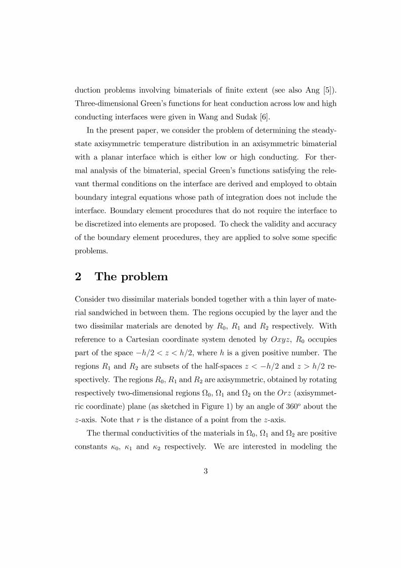
Consider two dissimilar materials bonded together with a thin layer of mate-

rial sandwiched in between them. The regions occupied by the layer and the

two dissimilar materials are denoted by 0, 1 and 2 respectively. With

reference to a Cartesian coordinate system denoted by , 0 occupies

part of the space −2 2, where is a given positive number. The

regions 1 and 2 are subsets of the half-spaces −2 and 2 re-

spectively. The regions 0 1 and2 are axisymmetric, obtained by rotating

respectively two-dimensional regions Ω0, Ω1 and Ω2 on the (axisymmet-

ric coordinate) plane (as sketched in Figure 1) by an angle of 360o about the

-axis. Note that is the distance of a point from the -axis.

The thermal conductivities of the materials in Ω0, Ω1 and Ω2 are positive

constants 0 1 and 2 respectively. We are interested in modeling the

3

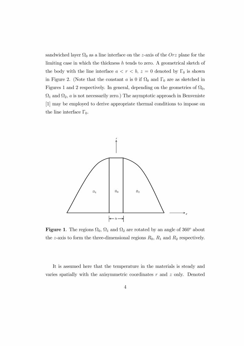
sandwiched layer Ω0 as a line interface on the -axis of the plane for the

limiting case in which the thickness tends to zero. A geometrical sketch of

the body with the line interface = 0 denoted by Γ0 is shown

in Figure 2. (Note that the constant is 0 if Ω0 and Γ0 are as sketched in

Figures 1 and 2 respectively. In general, depending on the geometries of Ω0,

Ω1 and Ω2, is not necessarily zero) The asymptotic approach in Benveniste

[1] may be employed to derive appropriate thermal conditions to impose on

the line interface Γ0.

Figure 1. The regions Ω0 Ω1 and Ω2 are rotated by an angle of 360o about

the -axis to form the three-dimensional regions 0, 1 and 2 respectively.

It is assumed here that the temperature in the materials is steady and

varies spatially with the axisymmetric coordinates and only. Denoted

4

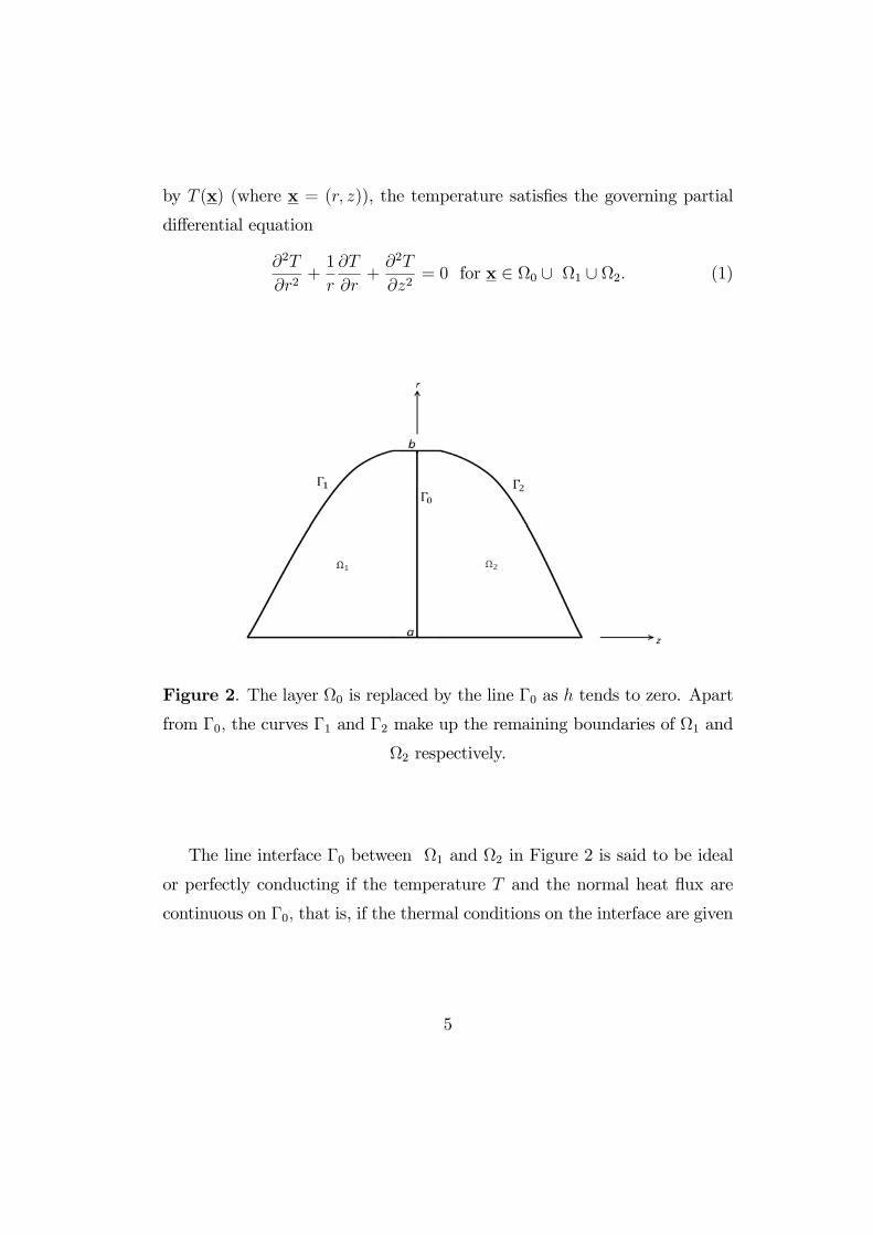
by (x) (where x = ( )), the temperature satisfies the governing partial

differential equation

2

2+1

+

2

2= 0 for x ∈ Ω0 ∪ Ω1 ∪ Ω2 (1)

Figure 2. The layer Ω0 is replaced by the line Γ0 as tends to zero. Apart

from Γ0 the curves Γ1 and Γ2 make up the remaining boundaries of Ω1 and

Ω2 respectively.

The line interface Γ0 between Ω1 and Ω2 in Figure 2 is said to be ideal

or perfectly conducting if the temperature and the normal heat flux are

continuous on Γ0 that is, if the thermal conditions on the interface are given

5

by ( 0+) = ( 0−)

2

¯=0+

= 1

¯=0−

⎫⎪⎪⎬⎪⎪⎭ for (2)

If the thermal conductivity 0 in the layer Ω0 is such that

0

→ (a finite positive constant) as → 0+, (3)

then the asymptotic analysis in Benveniste [1] may be used to derive the

following thermal conditions on Γ0:

2

¯=0+

= 1

¯=0−

[ ( 0+)− ( 0−)] = 2

¯=0+

⎫⎪⎪⎪⎪⎬⎪⎪⎪⎪⎭ for (4)

Note that (3) implies that 0 approaches zero as tends to zero. Thus,

(4) gives the thermal conditions on a layer with thickness and thermal con-

ductivity that tend to zero in such a way that there is a temperature jump

across opposite sides of the layer of vanishing thickness. A non-ideal conduct-

ing interface with such thermal conditions is said to be low conducting. The

line interface Γ0 between two materials as sketched in Figure 2 may be mod-

eled as low conducting if the interface is imperfect containing microscopic

gaps filled with air.

For another non-ideal conducting interface, if the thermal conductivity of

the layer Ω0 is given by

0→ (a finite positive constant) as → 0+, (5)

then the thermal conditions on Γ0 are given by

( 0+) = ( 0−)

2

¯=0+

− 1

¯=0−

= 2

2

¯=0

⎫⎪⎪⎬⎪⎪⎭ for (6)

6

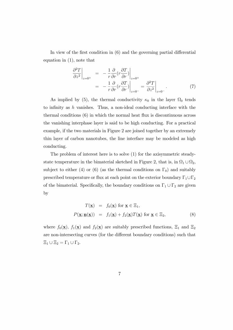
In view of the first condition in (6) and the governing partial differential

equation in (1), note that

2

2

¯=0+

= − 1

(

)

¯=0+

= − 1

(

)

¯=0−

=2

2

¯=0−

(7)

As implied by (5), the thermal conductivity 0 in the layer Ω0 tends

to infinity as vanishes. Thus, a non-ideal conducting interface with the

thermal conditions (6) in which the normal heat flux is discontinuous across

the vanishing interphase layer is said to be high conducting. For a practical

example, if the two materials in Figure 2 are joined together by an extremely

thin layer of carbon nanotubes, the line interface may be modeled as high

conducting.

The problem of interest here is to solve (1) for the axisymmetric steady-

state temperature in the bimaterial sketched in Figure 2, that is, in Ω1 ∪Ω2,subject to either (4) or (6) (as the thermal conditions on Γ0) and suitably

prescribed temperature or flux at each point on the exterior boundary Γ1∪Γ2of the bimaterial. Specifically, the boundary conditions on Γ1 ∪ Γ2 are givenby

(x) = 0(x) for x ∈ Ξ1

(x;n(x)) = 1(x) + 2(x) (x) for x ∈ Ξ2 (8)

where 0(x) 1(x) and 2(x) are suitably prescribed functions, Ξ1 and Ξ2

are non-intersecting curves (for the different boundary conditions) such that

Ξ1 ∪ Ξ2 = Γ1 ∪ Γ2.

7

3 Green’s function boundary element method

3.1 Boundary integral equations

The boundary integral equations for axisymmetric heat conduction governed

by (1) in the bimaterial sketched in Figure 2 are given by (see Brebbia et al

[7])

1(x0) (x0)

=

ZΓ1

( (x)1(x;x0;n(x))−0(x;x0) (x;n(x)))(x)

+

Z

( ( 0−)1( 0−;x0; 0 1)−0( 0

−;x0)

[ (x)]

¯=0−

)

for x0 = (0 0) ∈ Ω1 ∪ Γ0 ∪ Γ1 (9)

and

2(x0) (x0)

=

ZΓ2

( (x)1(x;x0;n(x))−0(x;x0) (x;n(x)))(x)

−Z

( ( 0+)1( 0+;x0; 0 1)−0( 0

+;x0)

[ (x)]

¯=0+

)

for x0 ∈ Ω2 ∪ Γ0 ∪ Γ2 (10)

where (x0) = 1 if x0 lies in the interior of Ω 1(x0) and 2(x0) are defined

by

1(x0) =

ZΓ1

1(x;x0;n(x))(x) +

Z

1( 0−;x0; 0 1)

for x0 = (0 0) ∈ Ω1 ∪ Γ0 ∪ Γ1 (11)

8

and

2(x0) =

ZΓ2

1(x;x0;n(x))(x)−Z

1( 0+;x0; 0 1)

for x0 ∈ Ω2 ∪ Γ0 ∪ Γ2 (12)

(x) denotes the length of an infinitesimal part of the curve Γ0∪Γ, n(x) =[(x) (x)] = (x)e +(x)e (e and e are the unit base vectors along

the and axes respectively) is the unit normal vector to Γ1 ∪ Γ2 (at the

point x) pointing out of Ω1 ∪Ω2, (x;n(x)) is the directional rate of changeof the axisymmetric temperature along the vector n(x) as defined by

(x;n(x)) = (x)

[ (x)] + (x)

[ (x)] (13)

and 0(x;x0) and 1(x;x0;n(x)) are given by

0(x;x0) = [()(0) +(−)(−0)](1)0 (x;x0) +

(2)0 (x;x0)

1(x;x0;n(x)) = [()(0) +(−)(−0)](1)1 (x;x0;n(x))

+(2)1 (x;x0;n(x))

(1)0 (x;x0) = −

((x;x0))

p(x;x0) + (; 0)

(1)1 (x;x0;n(x)) = −

1

p(x;x0) + (; 0)

× (x)2

[20 − 2 + (0 − )2

(x;x0)− (; 0)((x;x0))

−((x;x0))]

+ (x)0 −

(x;x0)− (; 0)((x;x0)) (14)

9

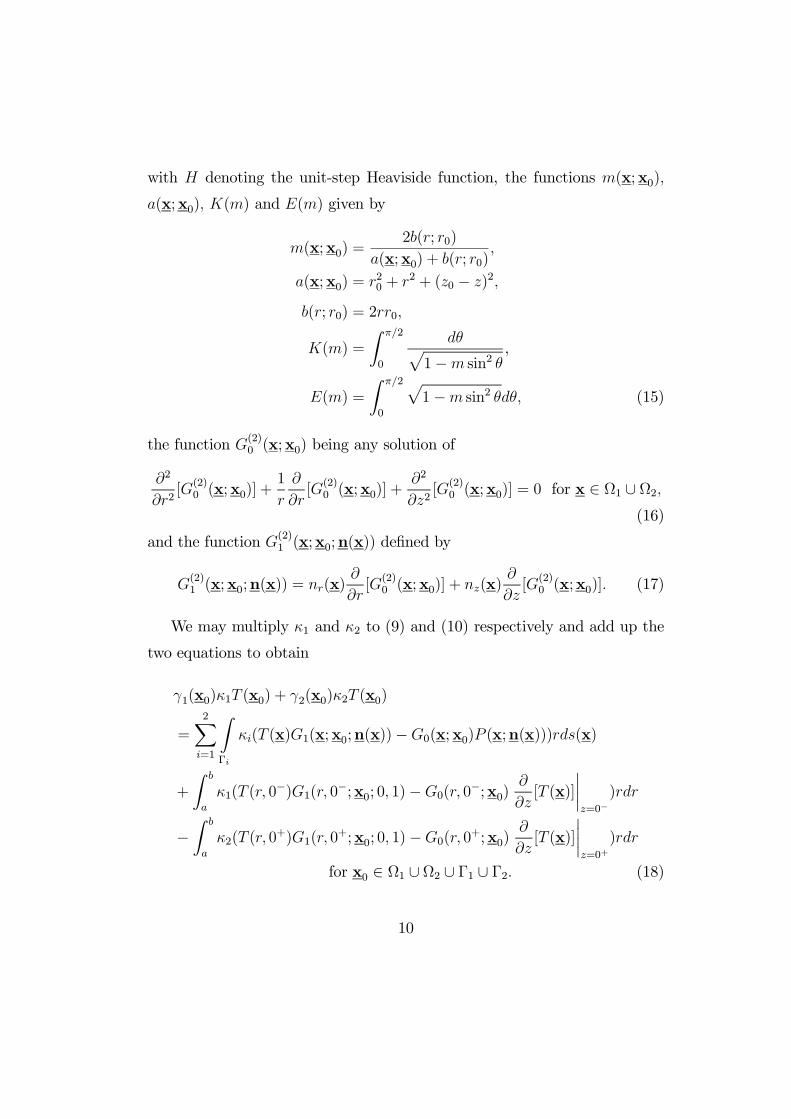
with denoting the unit-step Heaviside function, the functions (x;x0)

(x;x0) () and () given by

(x;x0) =2(; 0)

(x;x0) + (; 0)

(x;x0) = 20 + 2 + (0 − )2

(; 0) = 20

() =

Z 2

0

p1− sin2

,

() =

Z 2

0

p1− sin2 (15)

the function (2)0 (x;x0) being any solution of

2

2[

(2)0 (x;x0)] +

1

[

(2)0 (x;x0)] +

2

2[

(2)0 (x;x0)] = 0 for x ∈ Ω1 ∪ Ω2

(16)

and the function (2)1 (x;x0;n(x)) defined by

(2)1 (x;x0;n(x)) = (x)

[

(2)0 (x;x0)] + (x)

[

(2)0 (x;x0)] (17)

We may multiply 1 and 2 to (9) and (10) respectively and add up the

two equations to obtain

1(x0)1 (x0) + 2(x0)2 (x0)

=2X

=1

ZΓ

( (x)1(x;x0;n(x))−0(x;x0) (x;n(x)))(x)

+

Z

1( ( 0−)1( 0

−;x0; 0 1)−0( 0−;x0)

[ (x)]

¯=0−

)

−Z

2( ( 0+)1( 0

+;x0; 0 1)−0( 0+;x0)

[ (x)]

¯=0+

)

for x0 ∈ Ω1 ∪ Ω2 ∪ Γ1 ∪ Γ2 (18)

10

In general, we may take (2)0 (x;x0) in (14) to be

(2)0 (x;x0) = 0 Never-

theless, we may find it advantageous to solve (16) for (2)0 (x;x0) that satisfies

certain thermal conditions on the interface Γ0 of the bimaterial. As we shall

show below, a specially chosen(2)0 (x;x0)may be used in (14) for the integral

equation (18) such that the integrals over the interface Γ0 vanishes.

3.2 Green’s function for low conducting interface

For the case in which the interface Γ0 of the bimaterial is low conducting,

(2)0 (x;x0) is chosen in such a way that 0(x;x0) in (14) satisfies the inter-

facial conditions

20

¯=0+

= 10

¯=0−

[0( 0+;x0)−0( 0

−;x0))] = 20

¯=0+

⎫⎪⎪⎪⎪⎬⎪⎪⎪⎪⎭ for 0 ∞ (19)

The Green’s function 0(x;x0) satisfying (19) can be obtained by per-

forming an axial integration on the corresponding Green’s function for three-

dimensional heat conduction across a low conducting planar interface at

= 0 The analysis in Wang and Sudak [6] may be easily adapted to de-

rive the corresponding three-dimensional Green’s function. The derivation

is given in the Appendix. If we let = cos = sin = 0, = 0

and = 0 in the three-dimensional Green’s function for the low conducting

interface and integrate it with respect to from = 0 to = 2 we find that

the required axisymmetric Green’s function 0(x;x0) for low conducting Γ0

11

is given by (14) with

(2)0 (x;x0)

= (−0)(−)[(1)0 (x; 0−0)

−21

Z ∞

0

(1)0 (x; 0 − 0) exp(−

2(1 +

2

1))]

+()2

2

Z ∞

0

(1)0 (x; 0 0 − ) exp(−

2(1 +

2

1))

+(0)()[(1)0 (x; 0−0)

−22

Z ∞

0

(1)0 (x; 0−0 − ) exp(−

2(1 +

2

1))]

+(−)21

Z ∞

0

(1)0 (x; 0 0 + ) exp(−

2(1 +

2

1))

(20)

Note that (2)0 (x;x0) is obtained by integrating axially Φ∗( ; )

given in the Appendix by (A4) and (A11).

The function (2)1 (x;x0;n(x)) which corresponds to

(2)0 (x;x0) in (20) is

given by

(2)1 (x;x0;n(x))

= (−0)(−)[(1)1 (x; 0−0;n(x))−21

Z ∞

0

(1)1 (x; 0 − 0;n(x)) exp(−

2(1 +

2

1))]

+()2

2

Z ∞

0

(1)1 (x; 0 0 − ;n(x)) exp(−

2(1 +

2

1))

+(0)()[(1)1 (x; 0−0;n(x))

−22

Z ∞

0

(1)1 (x; 0−0 − ;n(x)) exp(−

2(1 +

2

1))]

+(−)21

Z ∞

0

(1)1 (x; 0 0 + ;n(x)) exp(−

2(1 +

2

1))

(21)

Using (4) and (19) for low conducting Γ0 we find that (18) can be reduced

12

to

1(x0)1 + 2(x0)2 (x0)

=2X

=1

ZΓ

( (x)1(x;x0;n(x))−0(x;x0) (x;n(x)))(x)

for x0 ∈ Ω1 ∪ Ω2 ∪ Γ1 ∪ Γ2 (22)

if 0(x;x0) and 1(x;x0;n(x)) are given by (14) with (20) and (21).

If (22) is used to derive a boundary element procedure for the numerical

solution of the problem stated in Section 2, it is not necessary to discretize

the low conducting interface Γ0 into boundary elements. Thus, the system

of linear algebraic equations in the boundary element formulation is smaller

with fewer unknowns.

3.3 Green’s function for high conducting interface

For the case in which the interface Γ0 of the bimaterial is high conduct-

ing, (2)0 (x;x0) is chosen in such a way that 0(x;x0) in (14) satisfies the

interfacial conditions

0( 0+;x0) = 0( 0

−;x0)

20

¯=0+

− 10

¯=0−

= 20

2

¯=0

⎫⎪⎪⎬⎪⎪⎭ for 0 ∞ (23)

The function (2)0 (x;x0) such that (23) holds is obtained by integrating

axially Φ∗( ; ) given by (A4) and (A19) in the Appendix (for three-

dimensional heat conduction across a high conducting planar interface at

13

= 0), that is,

(2)0 (x;x0)

= (−0)(−)[−(1)0 (x; 0−0)

+21

Z ∞

0

(1)0 (x; 0 − 0) exp(− 1

(1 + 2))]

+()21

Z ∞

0

(1)0 (x; 0 0 − ) exp(− 1

(1 + 2))

+(0)()[−(1)0 (x; 0−0)

+22

Z ∞

0

(1)0 (x; 0−0 − ) exp(− 1

(1 + 2))]

+(−)22

Z ∞

0

(1)0 (x; 0 0 + ) exp(− 1

(1 + 2))

(24)

The function (2)1 (x;x0;n(x)) which corresponds to

(2)0 (x;x0) in (24) is

given by

(2)1 (x;x0;n(x))

= (−0)(−)[−(1)1 (x; 0−0;n(x))

+21

Z ∞

0

(1)1 (x; 0 − 0;n(x)) exp(− 1

(1 + 2))]

+()21

Z ∞

0

(1)1 (x; 0 0 − ;n(x)) exp(− 1

(1 + 2))

+(0)()[−(1)1 (x; 0−0;n(x))

+22

Z ∞

0

(1)1 (x; 0−0 − ;n(x)) exp(− 1

(1 + 2))]

+(−)22

Z ∞

0

(1)1 (x; 0 0 + ;n(x)) exp(− 1

(1 + 2))

(25)

For high conducting Γ0, using (6), (7) and (23) and noting that

20

2

¯=0

= −1

(

[0( 0;x0)]) (26)

14

we find that (18) can be rewritten as

1(x0)1 (x0) + 2(x0)2 (x0)

=2X

=1

ZΓ

( (x)1(x;x0;n(x))−0(x;x0) (x;n(x)))(x)

+

Z

−0( 0;x0)1

(

)

¯=0+

+ ( 0)1

(

[0( 0;x0)])

for x0 ∈ Ω1 ∪ Ω2 ∪ Γ1 ∪ Γ2 (27)

Using integration by parts, we find thatZ

−0( 0;x0)1

(

)

¯=0+

+ ( 0)1

(

[0( 0;x0)])

= −0( 0;x0)

¯()=(0)

+ 0( 0;x0)

¯()=(0)

+ ( 0)

[0(x;x0)]

¯()=(0)

− ( 0)

[0(x;x0)]

¯()=(0)

(28)

It follows that (27) reduces to

1(x0)1 + 2(x0)2 (x0)− ( 0)

[0(x;x0)]

¯()=(0)

+ ( 0)

[0(x;x0)]

¯()=(0)

+ 0( 0;x0)

¯()=(0)

− 0( 0;x0)

¯()=(0)

=2X

=1

ZΓ

( (x)1(x;x0;n(x))−0(x;x0) (x;n(x)))(x)

for x0 ∈ Ω1 ∪ Ω2 ∪ Γ1 ∪ Γ2 (29)

Thus, the integral over the high conducting interface Γ0 vanishes if the

Green’s function 0(x;x0) is given by (14) with (2)0 (x;x0) in (25).

15

3.4 Boundary element procedures

In this section, we describe boundary element procedures for determining

(x) and (x;n(x)) (whichever is not known) on Γ1 ∪ Γ2. Once (x) and

(x;n(x)) are completely known on Γ1 ∪Γ2, we can obtain the temperatureat any point x0 in the interior of the domains by using 1(x0) = 1 and

2(x0) = 0 for x0 in the interior of Ω1 or 1(x0) = 0 and 2(x0) = 1 for x0 in

the interior of Ω2 in (22) (for low conducting interface) or in (29) (for high

conducting interface).

We discretize the boundary Γ1∪Γ2 into straight line elements denoted

by (1) (2) · · · (−1) and (). As (22) or (29) does not contain any

integral over the low conducting interface (because of the use of the special

Green’s function), we do not need to discretize the interface Γ0

For a simple approximation, and are taken to be constants over an

element of Γ1 ∪ Γ2, specifically (x) ' ()

(x;n(x)) ' ()

¾for x ∈ () ( = 1 2 · · · ) (30)

where () and () are constants.

Each boundary element is associated with only one unknown constant.

Specifically, if is specified over the element () according to the first line

of (8) then () is the unknown over (). On the other hand, if is given

by the second line of (8) over (), we can express () in terms of () and

regard () as the unknown constant over ()

16

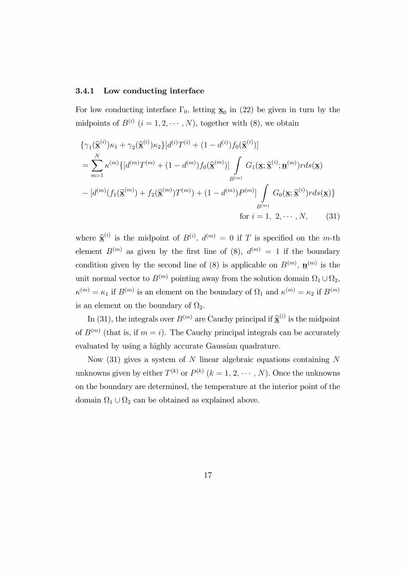
3.4.1 Low conducting interface

For low conducting interface Γ0 letting x0 in (22) be given in turn by the

midpoints of () ( = 1 2 · · · ), together with (8), we obtain

1(bx())1 + 2(bx())2[() () + (1− ())0(bx())]=

X=1

()[() () + (1− ())0(bx())] Z()

1(x; bx();n())(x)− [()(1(bx()) + 2(bx()) ()) + (1− ()) ()]

Z()

0(x; bx())(x)for = 1 2 · · · (31)

where bx() is the midpoint of () () = 0 if is specified on the -th

element () as given by the first line of (8), () = 1 if the boundary

condition given by the second line of (8) is applicable on () n() is the

unit normal vector to () pointing away from the solution domain Ω1 ∪Ω2,() = 1 if

() is an element on the boundary of Ω1 and () = 2 if ()

is an element on the boundary of Ω2

In (31), the integrals over () are Cauchy principal if bx() is the midpointof () (that is, if = ). The Cauchy principal integrals can be accurately

evaluated by using a highly accurate Gaussian quadrature.

Now (31) gives a system of linear algebraic equations containing

unknowns given by either () or () ( = 1, 2 · · · ) Once the unknownson the boundary are determined, the temperature at the interior point of the

domain Ω1 ∪ Ω2 can be obtained as explained above.

17

3.4.2 High conducting interface

For high conducting interface Γ0, if we proceed as before by collocating (29)

at the midpoint of each boundary element, we obtain

1(bx())1 + 2(bx())2[() () + (1− ())0(bx())]− ( 0)

[0(x;x0)]

¯()=(0)

+ ( 0)

[0(x;x0)]

¯()=(0)

+0( 0;x0)

¯()=(0)

− 0( 0;x0)

¯()=(0)

=X

=1

()[() () + (1− ())0(bx())] Z()

1(x; bx();n())(x)−[()(1(bx()) + 2(bx()) ()) + (1− ()) ()]

×Z

()

0(x; bx())(x)for = 1 2 · · · (32)

where () is as defined below (31).

The terms ( 0) ( 0)

¯()=(0)

and

¯()=(0)

in (32) are un-

known constants. They can, however, be approximated in terms of and

on boundary elements near ( 0) and/or ( 0). How the required approxi-

mations may be made depends on the geometries of the solution domains −see, for example, Problems 3 and 4 in Section 4 below. Thus, (32) can be

solved as a system of linear algebraic equations for unknowns given by

either () or () ( = 1 2 ).

4 Specific problems

Problem 1. To test the boundary element procedure for Γ0 that is low

conducting, consider the regions Ω1 and Ω2 as sketched in Figure 3. Note

18

that Ω1 and Ω2 are defined by the curves 2 + 2 = 4 and 2 + 2 = 1 and

the lines = 0, = 1, = 2 and = −1 on the plane. For a particularproblem take 1 = 1, 2 = 2 and = 1. The exterior boundary of Ω1 ∪ Ω2

is approximated using straight line elements.

The boundary conditions on the exterior boundary of Ω1 ∪ Ω2 are given

by (2 ; 1 0) = 4

(1 ;−1 0) = −2¾for − 1 0

(−1) = −2 + 23for 1 2

( ) =1

22 − 1

33 + 2 − 22

for 2 + 2 = 1 0 1

( ;1

21

2) = −1

23 − 22 + 3

42 + 2

for 2 + 2 = 4 0 2

Figure 3. A geometrical sketch of Problem 1 on the plane.

19

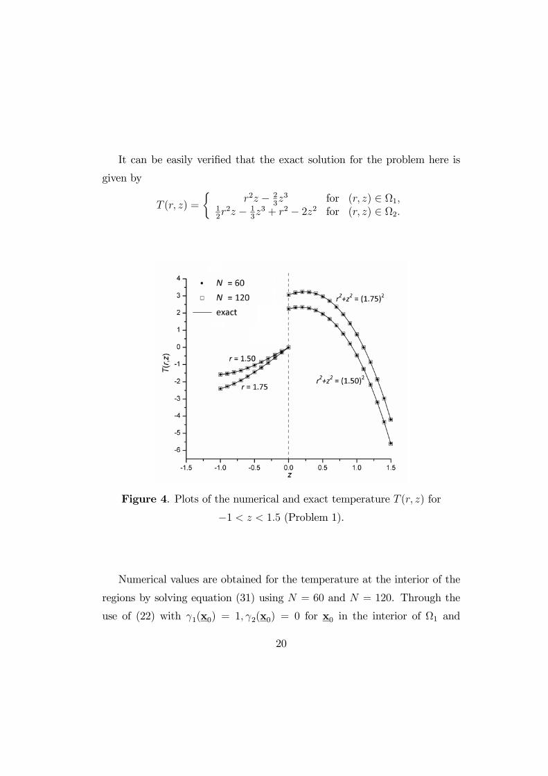
It can be easily verified that the exact solution for the problem here is

given by

( ) =

½2 − 2

33 for ( ) ∈ Ω1

122 − 1

33 + 2 − 22 for ( ) ∈ Ω2

Figure 4. Plots of the numerical and exact temperature ( ) for

−1 15 (Problem 1).

Numerical values are obtained for the temperature at the interior of the

regions by solving equation (31) using = 60 and = 120. Through the

use of (22) with 1(x0) = 1 2(x0) = 0 for x0 in the interior of Ω1 and

20

1(x0) = 0 2(x0) = 1 for x0 in the interior of Ω2, numerical values of the

temperature at = 15 and = 175 for −1 0 and at 2+ 2 = (175)2

and 2 + 2 = (15)2 for 0 15 are obtained and compared graphically

with the exact temperature in Figure 4. On the whole, the numerical and

exact temperature agree well with each other. Note that the gap in the graph

is due to the temperature jump across the interface Γ0 at = 0.

Problem 2. Consider now the case in which Ω1 and Ω2 are given by

Ω1 = ( ) : 0 ≤ 1 − 1 0Ω2 = ( ) : 0 ≤

3

2 0

3

2

as sketched in Figure 5. As in Problem 1, the interface Γ0 between Ω1 and

Ω2 is taken to be low conducting. Note that for this particular case the ex-

terior boundary of the bimaterial lies on part of the = 0 plane (that is,

1 32 = 0).

Figure 5. A geometrical sketch of Problem 2 on the plane.

21

For a particular problem, we take 1 = 1, 2 = 12 and = 1 and the

boundary conditions as

(1 ) = 4− 22 + 2 for − 1 0

(−1; 0−1) = −6 for 0 1

(3

2) = 2 +

13

2for 0

3

2

(3

2 ; 1 0) = 3 for 0

3

2

( 0) = 2 + 5 for 1 3

2

The exact solution for the particular problem here is given by

( ) =

½2 − 22 + 2 + 3 for ( ) ∈ Ω12 − 22 + 4 + 5 for ( ) ∈ Ω2

Table 1. Numerical and exact values of at selected interior points for

Problem 2.

Point = 25 = 50 = 100 = 200 Exact

(030−080) 021635 021094 021005 020996 021000(075−035) 261420 261655 261724 261743 261750(040−040) 203921 203947 203977 203992 204000(140 020) 760894 766118 767354 767800 768000(050 125) 711813 712282 712431 712478 712500(020 080) 694401 695498 695848 695954 696000

The exterior boundary of the bimaterial is discretized into straight line

elements. The numerical values of at various selected points in Ω1∪Ω2 arecomputed using (22) with 1(x0) = 1 and 2(x0) = 0 for x0 in the interior

of Ω1 and 1(x0) = 0 and 2(x0) = 1 for x0 in the interior of Ω2. They

22

are compared with the exact values in Table 1 for = 25 50 100 and 200

The numerical values are reasonably accurate and they converge to the exact

solution when the calculation is refined by reducing the sizes of the boundary

elements used (that is, when is increased from 25 to 200). All percentage

errors of the numerical values for = 200 are less than 005%.

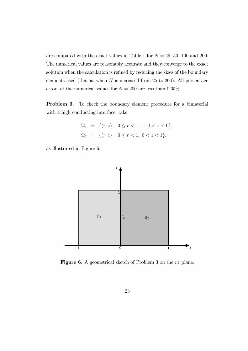
Problem 3. To check the boundary element procedure for a bimaterial

with a high conducting interface, take

Ω1 = ( ) : 0 ≤ 1 − 1 0Ω2 = ( ) : 0 ≤ 1 0 1

as illustrated in Figure 6.

Figure 6. A geometrical sketch of Problem 3 on the plane.

23

We take 1 = 6, 2 = 2, and = 74 and the boundary conditions as

(1 ; 1 0) = 4 + for − 1 0

(1 ) = 2 +1

2 − 42 − 3 for 0 1

(−1) = 322 − 17

3

( 1; 0 1) = 322 − 12

¾for 0 1

The exact solution of the particular problem here is given by

( ) =

½22 − 42 + 1

22 − 1

33 + 2 for ( ) ∈ Ω1

22 − 42 + 322 − 3 − for ( ) ∈ Ω2

The exterior boundary of the bimaterial is discretized into straight

line elements. To solve (32) as a system of linear algebraic equations in

unknowns, we have to approximate (1 0) and

¯()=(10)

in terms of

and on the boundary elements. (Note that for this particular problem,

= 0 and = 1.) If the exterior boundary is discretized in such a way

that the first and the last elements ((1) and () respectively) are of equal

length, lie on = 1 and have (1 0) as one of their endpoints, then we can

make the approximations

(1 0) ' 1

2( (1) + ())

¯()=(10)

' 1

2( (1) + ())

Numerical values of the temperature at selected interior points are com-

pared with the exact values in Table 2. On the whole, the numerical values

at the selected interior points are in good agreement with the exact solution

and improve in accuracy when is increased from 40 to 320 (again, calcu-

lation is refined by reducing the sizes of the boundary elements used). The

numerical results here also justify the above approximations for the terms

(1 0) and

¯()=(10)

in (32).

24

Table 2. Numerical and exact values of at selected interior points for

Problem 3.

Point = 40 = 80 = 160 = 320 Exact

(0500−0500) −152954 −152386 −152198 −152130 −152083(0200−0100) −017288 −016598 −016350 −016249 −016167(0700−0950) −447882 −447771 −447724 −447707 −447696(0900 0900) −214050 −215158 −215451 −215525 −215550(0100 0500) −159994 −159895 −159828 −159790 −159750(0750 0001) 110860 111827 112191 112347 112484

Problem 4. Problem 3 deals with relatively simple rectangular domains

on the -plane. For a more general test problem involving a high conducting

interface, we take here Ω1 with a slanted boundary = + 32 and Ω2 with

part of = 0 as its exterior boundary. A sketch of Ω1 ∪Ω2 is given in Figure7.

We take 1 = 1, 2 = 12 and = 18 and the boundary conditions on

the exterior boundary of Ω1 ∪ Ω2 as

( ) = 2 − 22 + 122 − 1

33

for = +3

2−1 0

(−1; 0−1) = −3− 122 for 0

1

2

( 2; 0 1) = −17 + 2 for 0 2

(2 ; 1 0) = 4(1 + ) for 0 2

( 0) = 2 for3

2 2

The exact solution of the problem here is given by

( ) =

½2 − 22 + 1

22 − 1

33 for ( ) ∈ Ω1

2 − 22 + 2 − 233 − for ( ) ∈ Ω2

25

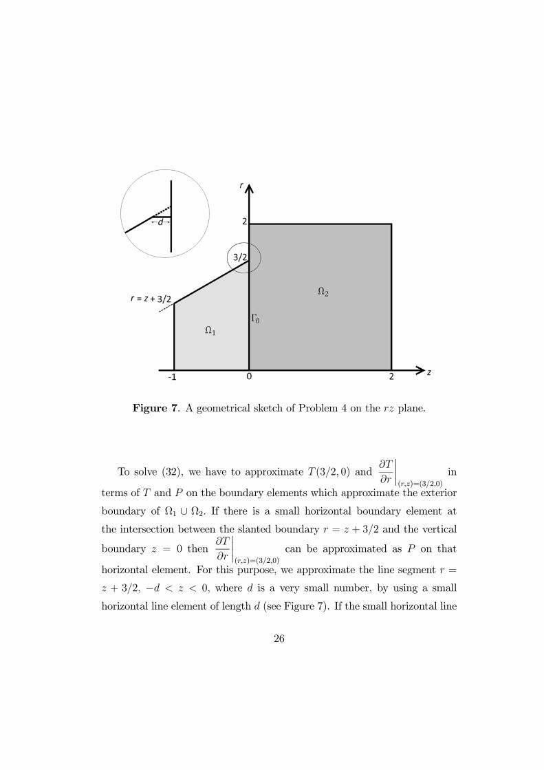
Figure 7. A geometrical sketch of Problem 4 on the plane.

To solve (32), we have to approximate (32 0) and

¯()=(320)

in

terms of and on the boundary elements which approximate the exterior

boundary of Ω1 ∪ Ω2 If there is a small horizontal boundary element at

the intersection between the slanted boundary = + 32 and the vertical

boundary = 0 then

¯()=(320)

can be approximated as on that

horizontal element. For this purpose, we approximate the line segment =

+ 32 − 0 where is a very small number, by using a small

horizontal line element of length (see Figure 7). If the small horizontal line

26

element is taken to be the first element (1) then

(32 0) ' (1)

¯()=(320)

' (1)

where (1) can be easily worked out from the given boundary conditions

(since is specified on = +32) and (1) is an unknown to be determined.

Figure 8. Plots of the numerical and exact boundary temperature (1 )

for −12 2 (Problem 4).

Numerical values are obtained for by using = 141 and = 281 with

= 00001The numerical results are compared graphically with the exact

solution as shown in Figure 8 and Figure 9. Figure 8 shows the temperature

along = 1 (−12 2) while Figure 9 captures the variation of the

27

temperature at = 1 and = 2 (0 2). On the whole, the numerical

and exact temperature values agree well with each other.

Figure 9. Plots of the numerical and exact boundary temperature ( )

for = 1 and = 2 (0 2) (Problem 4).

Problem 5. Here we consider a thermal management system modeled by

two homogeneous cylindrical solids as sketched in Figure 10. The regions

Ω1 and Ω2 model the computer chip and the heat sink respectively while

the interface Γ0 (line = 0, 0 2) represents a thin layer of carbon

nanotubes or nanocylinders of high thermal conductivity. We model the

interface Γ0 as high conducting.

28

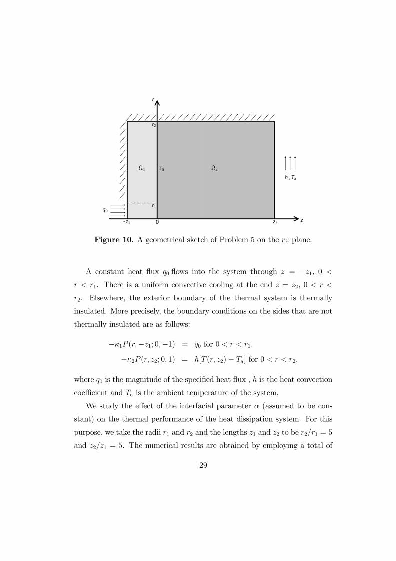
Figure 10. A geometrical sketch of Problem 5 on the plane.

A constant heat flux 0 flows into the system through = −1 0

1. There is a uniform convective cooling at the end = 2, 0

2. Elsewhere, the exterior boundary of the thermal system is thermally

insulated. More precisely, the boundary conditions on the sides that are not

thermally insulated are as follows:

−1 (−1; 0−1) = 0 for 0 1

−2 ( 2; 0 1) = [ ( 2)− a] for 0 2

where 0 is the magnitude of the specified heat flux , is the heat convection

coefficient and a is the ambient temperature of the system.

We study the effect of the interfacial parameter (assumed to be con-

stant) on the thermal performance of the heat dissipation system. For this

purpose, we take the radii 1 and 2 and the lengths 1 and 2 to be 21 = 5

and 21 = 5. The numerical results are obtained by employing a total of

29

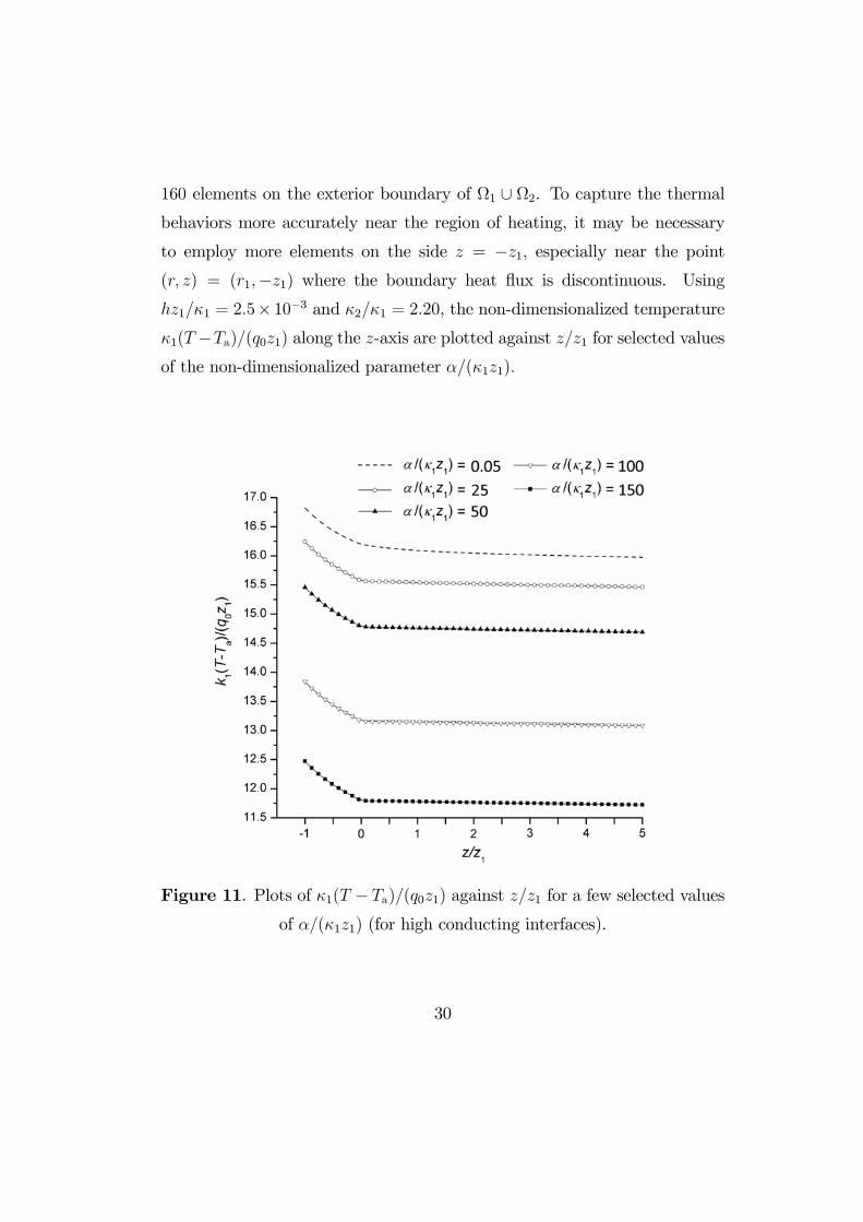
160 elements on the exterior boundary of Ω1 ∪ Ω2. To capture the thermal

behaviors more accurately near the region of heating, it may be necessary

to employ more elements on the side = −1 especially near the point( ) = (1−1) where the boundary heat flux is discontinuous. Using

11 = 25× 10−3 and 21 = 220, the non-dimensionalized temperature1( −a)(01) along the -axis are plotted against 1 for selected valuesof the non-dimensionalized parameter (11)

Figure 11. Plots of 1( − a)(01) against 1 for a few selected values

of (11) (for high conducting interfaces).

30

In Figure 11, the dashed line ((11) = 005) approximates the plot of

the non-dimensionalized temperature profile for the case in which the inter-

face between the chip and heat sink is nearly perfectly bonded (for perfectly

bonded or ideal interface, (11) = 0). As anticipated, at a given point

on the -axis, the non-dimensionalized temperature in both the computer

chip and heat sink decreases as (11) increases. Hence, the thin layer of

carbon nanotubes or nanocylinders of high thermal conductivity enhances

the heat dissipation performance of the system.

Still with 21 = 5, 21 = 5, 11 = 25 × 10−3 and 21 = 220,

we will now investigate the case whereby the interface between the chip

and the sink is filled with microscopic voids. We regard this interface as

low conducting. Again, we plot 1( − a)(01) against 1for selected

values of the non-dimensionalized parameter 11 as shown in Figure 12.

The dashed line (11 = 100) gives the temperature profile for the case

of a nearly ideal interface as there is negligible temperature jump across the

interface at = 0. Note that the dashed lines in both Figure 11 and Figure 12

give the temperature profile for a nearly perfect interface. The temperature

in the chip in Figure 12 is higher than that in Figure 11. Thus, the effect

of the low conducting interface on heat flow is opposite to that of the high

conducting one, that is, the low conducting interface obstructs rather than

enhance the heat flow from the chip into the sink. As expected, when the

obstruction of the heat flow is higher (that is, when 11 has a lower value),

the temperature jump across the interface at 1 = 0 is bigger. Also, the

differences between the temperature distributions for the different values of

11 are much smaller in the sink compared to those in the chip.

31

Figure 12. Plots of 1( − a)(01) against 1 for a few selected values

of (11) (for low conducting interfaces).

On the whole, Figures 11 and 12 summarize the effects of the three types

of interfaces − low conducting, perfectly conducting and high conducting

ones − on the thermal performance of the heat dissipation system in Figure

10.

5 Summary

Boundary element procedures based on special Green’s functions are pro-

posed for analyzing axisymmetric heat conduction across low conducting and

high conducting interfaces between two dissimilar materials. As the Green’s

32

functions satisfy the relevant interfacial conditions, the boundary element

procedures do not require the interfaces to be discretized into elements, giv-

ing rise to smaller systems of linear algebraic equations to be solved. The

procedures are applied to solve particular problems with known exact solu-

tions. The numerical solutions obtained confirm the validity of the Green’s

functions and the proposed Green’s function boundary element procedures.

References

[1] Y. Benveniste, On the decay of end effects in conduction phenomena:

a sandwich strip with imperfect interfaces of low or high conductivity,

Journal of Applied Physics 86 (1999) 1273-1279.

[2] A. Desai, J. Geer, B. Sammakia, Models of steady heat conduction in mul-

tiple cylindrical domains, Journal of Electronic Packaging-Transactions

of the ASME 128 (2006) 10-17.

[3] J. R. Berger, A. Karageorghis, The method of fundamental solutions for

heat conduction in layered materials. International Journal for Numerical

Methods in Engineering 45 (1999) 1681-1694.

[4] W. T. Ang, K. K. Choo, H. Fan, A Green’s function for steady-state

two-dimensional isotropic heat conduction across a homogeneously im-

perfect interface, Communications in Numerical Methods in Engineering

20 (2004) 391-399.

[5] W. T. Ang, Non-steady state heat conduction across an imperfect inter-

face: a dual-reciprocity boundary element approach, Engineering Analy-

sis with Boundary Elements 30 (2006) 781-789.

33

[6] X. Wang, L. J. Sudak, 3D Green’s functions for a steady point heat source

interacting with a homogeneous imperfect interface, Journal of Mechanics

of Materials and Structures 1 (2006) 1269-1280.

[7] C. A. Brebbia, J. C. F. Telles, L. C. Wrobel, Boundary Element

Techniques, Theory and Applications in Engineering, Springer-Verlag,

Berlin/Heidelberg, 1984.

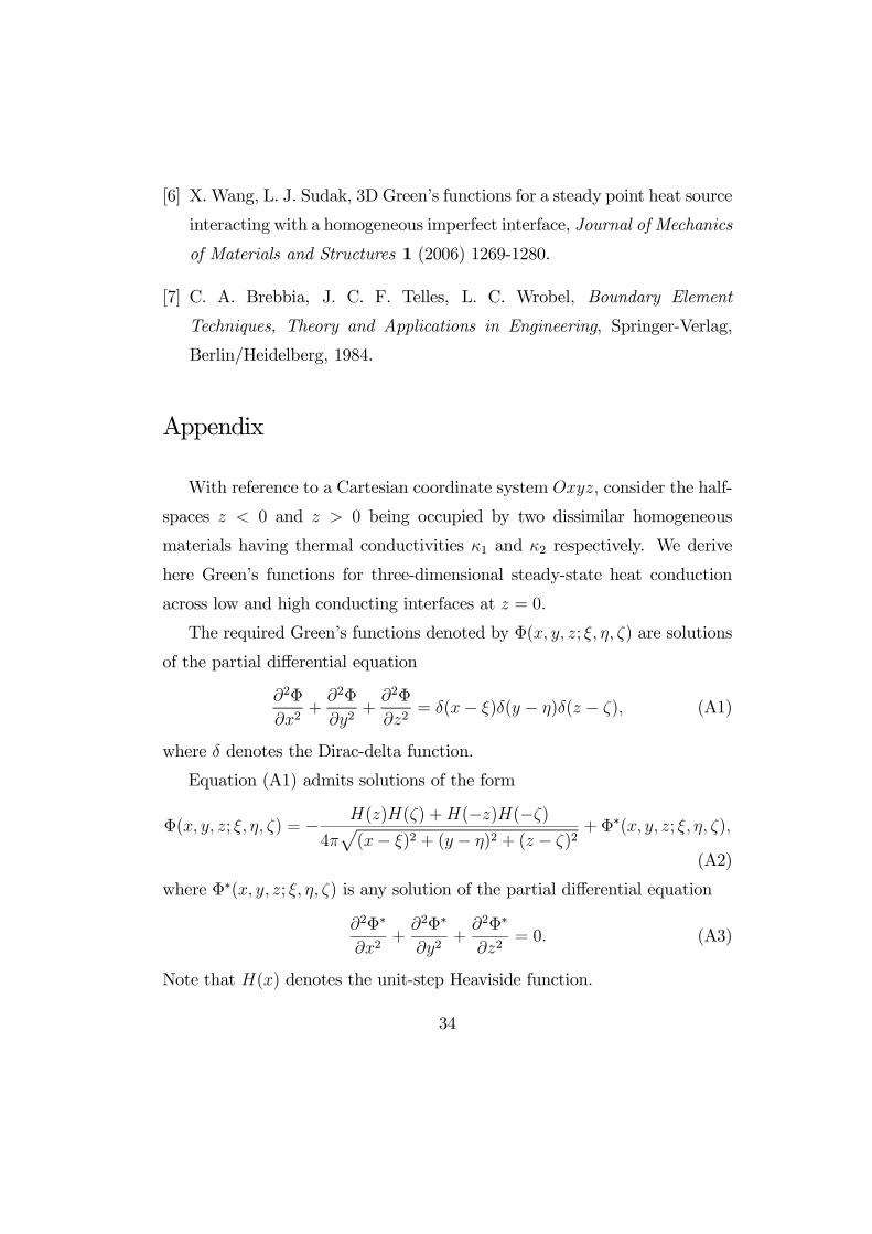
Appendix

With reference to a Cartesian coordinate system consider the half-

spaces 0 and 0 being occupied by two dissimilar homogeneous

materials having thermal conductivities 1 and 2 respectively. We derive

here Green’s functions for three-dimensional steady-state heat conduction

across low and high conducting interfaces at = 0

The required Green’s functions denoted by Φ( ; ) are solutions

of the partial differential equation

2Φ

2+

2Φ

2+

2Φ

2= (− )( − )( − ) (A1)

where denotes the Dirac-delta function.

Equation (A1) admits solutions of the form

Φ( ; ) = − ()() +(−)(−)4p(− )2 + ( − )2 + ( − )2

+ Φ∗( ; )

(A2)

where Φ∗( ; ) is any solution of the partial differential equation

2Φ∗

2+

2Φ∗

2+

2Φ∗

2= 0 (A3)

Note that () denotes the unit-step Heaviside function.

34

The function Φ∗( ; ) are given in Wang and Sudak [6] for low

and high conducting interfaces for = 0 The analysis in [6] can be modified

to include the case where 6= 0 We take Φ∗( ; ) to be of the form

Φ∗( ; )

= (−)(−)[ 0

4p(− )2 + ( − )2 + ( + )2

+1

Z ∞

0

exp(−3)p(− )2 + ( − )2 + ( + − )2

]

+()2

Z ∞

0

exp(−3)p(− )2 + ( − )2 + ( − + )2

+()()[ 0

4p(− )2 + ( − )2 + ( + )2

+1

Z ∞

0

exp(−3)p(− )2 + ( − )2 + ( + + )2

]

+(−)2Z ∞

0

exp(−3)p(− )2 + ( − )2 + ( − − )2

(A4)

where 0, 1 2 3 0 1 2 and 3 are constants. We assume a priori that

3 and 3 are positive constants so that the improper integrals over [0∞) in(A4) exist.

It may be easily verified that (A4) is a solution of (A3) at all points

( ) in space. The constants 0, 1 2 3 0 1 2 and 3 are chosen to

satisfy the conditions on the interfacial conditions.

Low conducting interface

For the case in which = 0 is low conducting, Φ( ; ) is required

to satisfy the interfacial conditions

1

[Φ( ; )]

¯=0−

= 2

[Φ( ; )]

¯=0+

35

[Φ( 0+; )− Φ( 0−; )] = 2

[Φ( ; )]

¯=0+

(A5)

If we take 0 = 0 = −1, the condition on the first line of (A5) is satisfiedif

−11 = 22

−12 = 21 (A6)

For 0 the condition on the second line of (A5) is satisfied if

(2 − 1)

Z ∞

0

exp(−3)p(− )2 + ( − )2 + (− )2

+

2q(− )2 + ( − )2 + 2

= −22Z ∞

0

(− ) exp(−3)[(− )2 + ( − )2 + (− )2]32

(A7)

Using the integration by parts, we obtainZ(− ) exp(−3)

[(− )2 + ( − )2 + (− )2]32

= − exp(−3)[(− )2 + ( − )2 + (− )2]12

−3Z

exp(−3)p(− )2 + ( − )2 + (− )2

(A8)

From (A7) and (A8), it follows that

−222 =

223 = (2 − 1) (A9)

Similarly, for 0, we obtain

221 =

−213 = (−1 + 2) (A10)

36

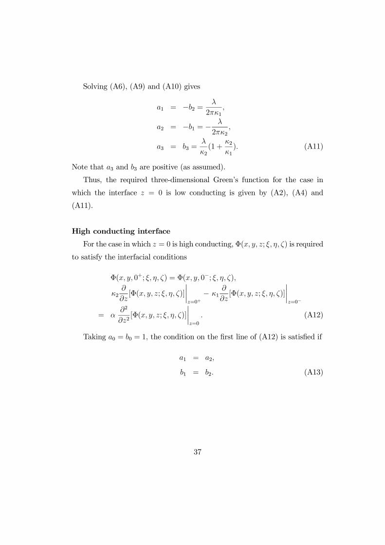
Solving (A6), (A9) and (A10) gives

1 = −2 =

21

2 = −1 = −

22

3 = 3 =

2(1 +

2

1) (A11)

Note that 3 and 3 are positive (as assumed).

Thus, the required three-dimensional Green’s function for the case in

which the interface = 0 is low conducting is given by (A2), (A4) and

(A11).

High conducting interface

For the case in which = 0 is high conducting, Φ( ; ) is required

to satisfy the interfacial conditions

Φ( 0+; ) = Φ( 0−; )

2

[Φ( ; )]

¯=0+

− 1

[Φ( ; )]

¯=0−

= 2

2[Φ( ; )]

¯=0

(A12)

Taking 0 = 0 = 1 the condition on the first line of (A12) is satisfied if

1 = 2

1 = 2 (A13)

37

For 0 the condition on the second line of (A12) is satisfied if

−(11 + 22)

Z ∞

0

(− ) exp(−3)[(− )2 + ( − )2 + (− )2]32

+1

2[(− )2 + ( − )2 + 2]32

= 2

Z ∞

0

exp(−3) 2

2[

1p(− )2 + ( − )2 + (− )2

]

¯¯=0

(A14)

Using integration by parts and the relation

2

2[

1p(− )2 + ( − )2 + ( − + )2

]

¯¯=0

=2

2[

1p(− )2 + ( − )2 + (− )2

] (A15)

we obtain

1

2[(− )2 + ( − )2 + 2]32− (11 + 22)q

(− )2 + ( − )2 + 2

+3(11 + 22)

Z ∞

0

exp(−3)p(− )2 + ( − )2 + (− )2

= 2−

[(− )2 + ( − )2 + 2]32− 3q

(− )2 + ( − )2 + 2

+23

Z ∞

0

exp(−3)p(− )2 + ( − )2 + (− )2

(A16)

From (A16), it follows that

1 = −22(11 + 22) = 23 (A17)

38

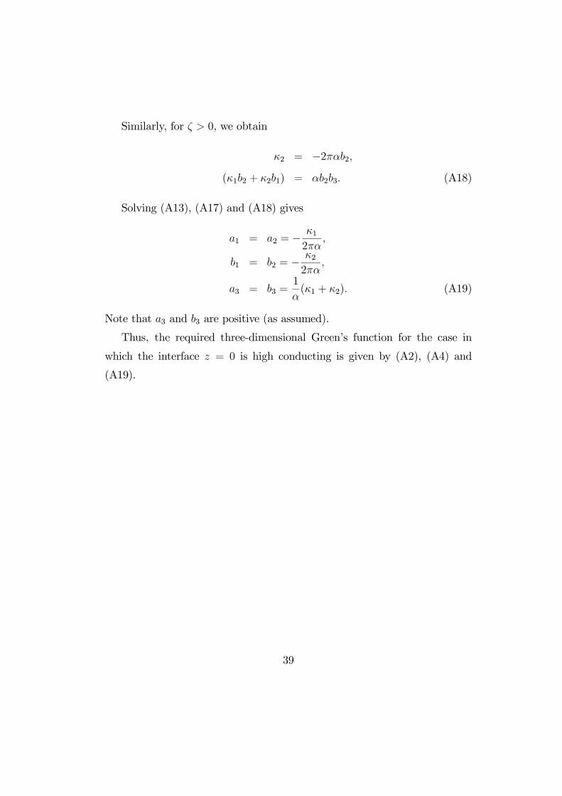
Similarly, for 0, we obtain

2 = −22(12 + 21) = 23 (A18)

Solving (A13), (A17) and (A18) gives

1 = 2 = − 1

2

1 = 2 = − 2

2

3 = 3 =1

(1 + 2) (A19)

Note that 3 and 3 are positive (as assumed).

Thus, the required three-dimensional Green’s function for the case in

which the interface = 0 is high conducting is given by (A2), (A4) and

(A19).

39