Spatial weighting in laboratory incoherent light scattering experiments

Spatial weighting in laboratory incoherent light scattering experiments

J. F. Kusters, Barry J. Rye, and Andrew C. Walker

Diffraction-based calculations of the relative spatial weighting of the observed volume in incoherent scattering experiments, applicable to both direct detection and heterodyne systems and arbitrary transmitter and receiver profiles, have been largely confirmed in laboratory measurements using a CO2 laser. The results indicate that heterodyne systems have superior spatial resolution at small scattering angles for a given detector geometry and permit quantitative assessment of this and the greater sensitivity of coherent systems to misalignment.

I. Introduction The spatial weighting of the observed volume in an

incoherent scattering experiment is crucial to calibration of the system and determination of both spatial and angular resolution. Different expressions are obtained for the weighting dependent on whether direct or optical heterodyne detection is used. In both cases the result can be expressed in terms of the overlap of the fields of view (FOV) of the transmitter and receiver. For direct detection geometrical optics often suffices to calculate the FOV but if the etendue of the system is small (e.g., for angular resolution) diffraction must be taken into account, as is always the case for heterodyning. The topic of this paper is experimental confirmation of spatial weighting calculations in the diffraction-dominated regime.

The motivation for this study was a proposed small-angle incoherent scattering measurement on the Eura-tom joint European tokamak (JET) using a pulsed CO2 laser source and Ge:Cu heterodyne detection system.1– 3 In this diagnostic the spectrum of scattered light provides information on the plasma particles (e.g., ion temperature, density) and on the level of turbulence in the plasma.4,5 The Doppler shifts generating the spectrum are dependent on scattering angle. If the scattering volume is finite both incident and scattered

Andrew Walker is with UKAEA Culham Laboratory, Abingdon, Oxfordshire 0X14 3DB, U.K.; the other authors were with University of Hull, Department of Applied Physics, Hull, N. Humberside HU6, 7RX, U.K.

Received 12 February 1988. 0003-6935/89/040657-08$02.00/0. © 1989 Optical Society of America.

beams have finite angular spread so the scattering angle is not precisely defined. There is thus a tradeoff between spatial and angular resolution. In addition to this fundamental problem, there is also the variation in spatial weighting arising from the FOV overlap of transmitter and receiver that are noncoax-ial.

Analytical calculations have been given by Holz-hauer and Massig6 for Gaussian beam profiles, which in some sense optimize the trade-off. However in practice the choice between various possible transmitter/receiver geometries does not only depend on spatial weighting considerations. For example, demands on the data processing are significantly relaxed by maximizing the transmitter power,7 which may be accomplished by use of an unstable cavity laser giving an annular output, and by maximizing the receiver acceptance, which may be achieved for small scattering angles by the use of annular spatial filters in a receiver aligned coaxially with the transmitter.8 Both of these improvements were in mind for the JET experiment and Gaussian optics could therefore not be used. Moreover, with plasma containment devices it is not unusual for difficulties in accessing the plasma to be a significant constraint in the choice of scattering geometry so that computational optical design is called for.

Much modeling work of the type required has been done in the context of optical radar (coherent lidar). Diffraction theory has been used to obtain expressions for an effective heterodyne receiver area; of particular relevance here, the range (or scattering volume) dependence of this quantity has been exploited to provide systems using continuous laser sources with a degree of range resolution,9 and calculations have been made of the performance of long-range systems including the contribution of primary aberrations in the optics.10

15 February 1989 / Vol. 28, No. 4/ APPLIED OPTICS 657

This provides the basis for the present analysis described in Sec. II. To supplement the work of Holz-hauer and Massig6 computer programs were prepared that permitted numerical calculation of the spatial weighting in arbitrary transmitter and receiver geometries. The scattering volume is regarded as a stack of scattering planes and the relative contribution of these planes is evaluated; thus we estimate the weighting of scattering planes as opposed to the study of the line weighting observed by Jones et al.11 As the scattering is incoherent, the signal powers obtained from the different scattering planes are additive.

Our approach makes use of the equations of Fourier optics12-13 which relate functions of the optical fields within any plane (here in the scattering volume) and their spatial frequency spectrum. In physical terms the latter describes the angular spread. From this point of view (i) the trade-off between spatial and angular resolution mentioned above is an example of the reciprocity relation existing between the width of functions in the two transform domains and (ii) the spatial spectrum of the scattering system can be computed as the convolution of the spectra of the transmitter and reciprocal receiver. Here however we do not go this far; we simply use the expressions for the total scattered light intensity written (from choice) in the spatial frequency domain to evaluate the spatial weighting of the scattering volume.

In Sec. III comparisons between our numerical data and experimental observations of the scattering from a rotating rough target in a simple noncoaxial geometry with small-angle scattering angle and receiver spatial filtering are described. The beam profiles used were Gaussian but were significantly truncated. Both heterodyning and direct detection were used and computations for the latter employed wave rather than geometrical optics because of the small detector size. The comparison of heterodyne and direct detection data is especially instructive in that it directly indicates the alignment-dependent heterodyne efficiency of the coherent receiver. These results have been previously reported in conference publications14,15 and have been the subject of a thesis.16

II. Computer Simulation In Secs. B and C expressions equivalent to the power

received from a given plane using, respectively, heterodyne and direct detection are found in terms of integrals over the spatial spectra of the optical fields in that plane. First, in Sec. A, the concepts and notation that are used to describe the optical fields and their spectra are defined.

A. Transmitter and Reciprocal Receiver Geometry For the purpose of describing the simple optics used

in the experiments below, the optical systems of the transmitter and receiver are each modeled as a thin lens with an entrance pupil stop placed within the focal distance F (Fig. 1). In the transmitter this optics is illuminated by the laser source. To quantify receiver FOV the concept of the reciprocal receiver is used,

658 APPLIED OPTICS / Vol. 28, No. 4 / 15 February 1989

Fig. 1. Geometry used in computation of transmitter and reciprocal receiver spatial frequency spectrum.

Fig. 2. Equivalent optics of Fig. 1, showing exit pupil.

whereby the antenna properties are defined by a notional beam propagating backward through the optics. For heterodyning this beam is originated (according to Siegman's antenna theorem17) by the phase conjugate of that part of the local oscillator beam incident on the photodetector, the latter therefore acting as a (notional) source. Construction of the reciprocal receiver for direct detection incoherent scattering systems is discussed in Sec. C. Use below of the word receiver in isolation implies the actual receiver, with light propagating toward the photodetector.

The definition of the exit pupil as the image of the entrance pupil in the lens enables the equivalent optics of Fig. 2 to be defined. Within the equivalent system the problem of computing the fields in a scattering plane is reduced to the analysis of free-space propagation between the plane and the exit pupil.

This propagation problem is further simplified by consideration of the fields on a Gaussian reference sphere12 defined to be tangential to the exit pupil of the focusing optics on the optical axis and centered on the scattering plane of interest (Fig. 2). The irradiance I in the scattering plane as a function of lateral displacement s is given, for example, by the 2-D Fourier transform:

of the autocorrelation function

of the reference sphere fields U(f). The latter are written as a function of the spatial frequency

rather than as a function of the displacement b in the exit pupil plane in order to bring out the Fourier transform nature of Eq. (1). P represents the power passing through the pupil and λ is the optical wavelength. The autocorrelation functions µ give the spatial spectral profile of the irradiance and as used here are normalized such that µ(0) = 1.

In many lidar applications both entrance and exit pupils of the receiver are located in the plane of the receiving lens or mirror as this has the widest aperture in the optical system. Use has however been made of receiver focal plane stops (x1 = F in Fig. 1) to attenuate near-field returns and reduce the dynamic range of the signal.18 Although geometrical optics was used to analyze this system, such an arrangement is conventional in the laboratory spatial filtering experiments analyzed using diffraction theory.13 The exit pupil is located at infinity so identification of spatial frequency with angular direction is clear-cut, and the focal plane is often referred to as the frequency plane as this is where filtering apertures are positioned. It may be noted however that use of the spatial frequency concept arises from the existence of transform relations such as Eq. (1) and is not dependent on the geometry of any particular optical system; it follows that here we can relate and combine functions in the spatial frequency domain calculated using the parameters of the transmitter and reciprocal receiver even if the geometries of these are quite different and regardless of the positions of the pupils.

We now turn to the relationship between the optical system variables of Fig. 1 and the equivalent optics of Fig. 2. The exit pupil reference sphere fields are written in terms of spatial frequency as

where \U(f)\ describes the amplitude profile and φ(f) is the aberration function, defined as the radial path difference between the transmitter or reciprocal receiver wavefront at the exit pupil and the reference sphere.10,12 As the entrance and exit pupils are mutual images their fields are identical apart from scaling due to magnification and phase differences arising from curvature and optical component aberrations. \U(f)\ can therefore be computed by consideration of the free-space propagation between the source plane and the entrance pupil.

The relationship between spatial frequency in the exit pupil and the optical system variables of Fig. 1 is found as follows. The lens equation yields

where as x1 < F and u < F the sign convention is that all distances are positive. Substituting Eq. (3), noting that displacements in the entrance pupil b1 scale as b1 b = x1/x, and eliminating the variables x and b that are not known experimentally, we find

|U(f)| I is calculated by finding the field at displacement b1 in the entrance pupil and assigning it to the frequency f given by Eq. (5). As the sources are small the entrance pupil is in the far field of the source and is illuminated by a spherical wave of radius of curvature u – x1 and Gaussian profile. The truncation factor (the ratio of the beam waist to the pupil radius) is a variable parameter in the program.10

Since the wavefront just described lies in the entrance pupil reference sphere, in the absence of component aberrations the wavefront in the exit pupil will lie on a sphere of radius x + v (Fig. 2), converging on the focusing plane. If the scattering plane is coincident with the focusing plane this sphere is also the reference sphere so the aberration function in Eq. (4) will be zero (in this case the two reference sphere fields are measures through Eq. (3) of the frequency spectrum of the source and its image, which are identical). For other scattering planes account can be taken of the phase difference between the wavefront and the reference sphere due to curvature by use of the defect of focus aberration function10,12

In the transmitter (variables subscripted T) the lens and pupil planes were coincident [(x)T = 0, (b1)T = bT] giving, in Eqs. (5) and (6),

while for the reciprocal receiver (subscript R), where a focal plane stop was used, (x1)R = F and

B. Heterodyne Receiver An approximation for the effective receiver area in a

heterodyne experiment Ahet, valid for small scattering angles, was derived previously.10 To include the case where a focal plane stop is used and the receiver entrance pupil is at infinity, it is more meaningful to use the solid angle Ωhet subtended by the receiver at the scattering plane rather than Ahet itself. Making this change we have

Here the displacement of the transmitted beam profile relative to the receiver axis is included by means of the exponential term arising from use of the shift theorem,10 S being defined as in Fig. 3, and R = xR + rR.


Fig. 3. Schematic of low angle scattering geometry with receiver focal plane stops for angle selection.

The subscript L refers to the (notional) backpropagat-ed local oscillator (BPLO) beam that defines the reciprocal receiver FOV, PL being the power falling on the photodetector. Given the normalization properties of the spectral functions forming the integrand in Eq. (9), the integral is a measure of its width.19

As in Ref. 10, Eq. (9) was evaluated here by direct and time-consuming computation of the correlation functions using Eqs. (2) and (4) and subsequent numerical integration.

C. Direct Detection The mean detected power can be written as

where a is a displacement vector on the photodetector surface, A D is the photodetector area, and GD(a) is a (real) weighting function to describe the photodetector efficiency and geometry, normalized so that

ID(a) is the speckle-averaged signal irradiance. It is possible to develop frequency plane expressions by writing ID = UD(a) U*D(a) and basing reciprocal receiver properties on the backpropagated signal field U*D(a)G*D(a). However it is somewhat simpler to proceed from the standard Fourier optics result, that for incoherent imaging13 ID(a) is given by the 2-D convolution Is(a) ** IR(a), where Is(a) is a perfectly imaged profile of the source (here the demagnified scattering plane irradiance profile as determined by the transmitted beam parameters) and IR(a) is the point spread function13 (PSF) of the receiver optics.

The overall mean received power is

In the usual scattering (or lidar) equations this is written as the product of the area A R of the receiver entrance pupil with a receiver transmission loss factor. As we wish to take explicit account of truncation at the detector, we define an effective direct detection receiver area as


The power theorem can be used to rewrite this expression in terms of parameters defined on a reference sphere that is centered on the reciprocal receiver entrance pupil as follows:

where µ(f) can be identified with the receiver optical transfer function for incoherent illumination13; gD(f) is the Fourier transform of GD (a) and the product μs(f)μR(f) is that of ID(a) as defined above.19

To put this equation into a form in which it can be compared directly with Eq. (9), note that µs,R(f = 0) = 1 and that µs can be replaced by µr(f) exp(j2πf • S) since each expression is the (normalized) frequency transform of the transmitted beam irradiance IT(s) [see Eqs. (1) and (9) and Fig. 313]. Also, if we choose to regard µR(f) as the property of a reciprocal receiver, i.e., to regard the propagation as being from the photodetector toward the source, the sign convention for phase lags has to be reversed and µR(f) replaced by µ*R(f). The equation then becomes

The product µ*R(f)gD(f) takes the place of the BPLO term in Eq. (9) and together with A D defines the antenna properties of a direct detection receiver; if the detector weighting function GD(a) is symmetrical, g*D(f) is also real19 and is merely an aperturing term, the phase contribution then coming entirely from µ*R(f). The expression usually associated with direct detection is obtained if the photodetector does not reduce the signal, i.e., if it is both sufficiently large to take in all the received signal and uniform in response across its surface, so gD(f) → (1/AD)δ(f) and the integral in the numerator of Eq. (13) becomes 1/AD;, thus Adir → AR as would be expected in the geometrical optics limit, provided there is not vignetting within the receiver.

The similarity between ]Eqs. (9) and (14) facilitates comparative simulation of direct detection and heterodyne experiments especially if absolute measurements are not attempted, so the factors in the two equations outside the integrals are immaterial to the comparison. For heterodyning µL(f) is calculated using the (Gaussian) profile of the BPLO, while for the direct detection simulation µR(f) uses a uniform profile. In the experiments described below the photodetector was rectangular but circular stops were used to reduce its aperture; for a circular aperture of diameter d,

and19

where J1(x) is the first-order Bessel function and ll(x) is the top-hat function II(|x| < 1) = 1, II(|x| ≥ 1) = 0.

III. Experimental Simulation

A. Layout The experimental arrangement was based on a half-

scale simulation of the proposed tokamak system and is described with the help of Fig. 4.

The transmitter laser source was a continuous Edinburgh Instrument CO2 laser giving an output of ~3 W in a TEM00 mode on 10P(20). This was focused through a single lens with a stop A1 that reduced the power transmitted by ~50%. A number of scattering targets were tried, including disks of polythene sheet, alcohol aerosol sprays, fine sand dropped through the scattering volume, and structures made of fine wires. The best results were obtained by rotating through the scattering volume a disk of KBr, one surface of which had been sandblasted until the scattering signal statistics appeared reasonably smooth and nonspikey. The axis of the disk lay in the scattering plane so scattered light experienced negligible Doppler shift. Sectors of the disk were covered so that it acted as a beam chopper as well as a scatterer. Data were confirmed by use of separate observations of scattering from different radial positions on the disk surface. This target could be adjusted a distance of ~25 cm in each direction along the axis of the transmitted beam around the position of focus. The scattering angle was adjusted to be 0.75°.

On the receiver side an off-axis mirror MS together with two lenses L1 and L2 formed an image of this plane on the surface of a Labimex room temperature CMT photodetector. The scattered light beam was filtered by means of the focal plane (angle selective) aperture A3 within this receiver. For the direct detection work a further image stop A2 was introduced in a plane conjugate to both the central scattering plane and the photodetector surface to reduce by a factor of about a half the effective area of the latter. For heterodyning, a second cw CO2 laser was used as a local oscillator, the beam being combined with the scattered light on a NaCl beam splitter also within the receiver optics. The beam was initially Gaussian but suffered a 50% truncation at stop A3. The only further attenuation of this beam arose at the beam splitter. The beam dump could be removed and mirror M6 introduced to reflect a local oscillator beam through the focusing plane of the transmitter laser to facilitate alignment. This was found to be very critical when optimizing the heterodyne signal, and it was helpful to use a carbon sheet viewed through an infrared camera to determine the position of the two beams. The cw lasers were stabilized optogalvanically with a frequency offset of 4-5 MHz.

The processing system for the coherent receiver is depicted in Fig. 5. For direct detection the system was essentially the same except that the rectifier (a 50-Ω square-law detector followed by a low pass filter) was not of course needed. Amplification was achieved with a Tektronix AM502 (33-dB gain) for direct detection and an in-house unit based on a ZN459 chip with 56-dB gain and a bandwidth of 300 kHz for heterodyn-

Fig. 4. Experimental optics layout; the numbers F are focal lengths in centimeters.

Fig. 5. Heterodyne detection receiver circuitry.

Fig. 6. Plot of heterodyne receiver signal strength, expressed as an effective receiver solid angle, as a function of axial distance: —, simulated data; +, experimental points. The values indicated on

the ordinate are the computed solid angle in microsteradians.

ing. The phase-locked amplifier was used for quantitative estimation of the signal, a reference at 122 Hz being taken from the scattering disk; the output time constant was 0.1 s.

B. Heterodyne Experiments The axial dependence of the heterodyne return is

shown in Fig. 6, together with the prediction of the computer simulation. The two curves are fitted only in height at their maxima at it is the match between their halfwidths that is of principal interest, and the axial distances are of course known absolutely in either case. In the experimental data there is a wing stretching toward the transmitter in which the signal is larger than the prediction, whereas toward the receiver the converse is true. The deviation is therefore nonsymmetrical and cannot be explained by a simple angular error. Figure 7 shows the same plot with the signal plotted on a logarithmic scale, from which it is apparent that the full width at half-maximum (FWHM)


Fig. 7. Same as Fig. 6, with a logarithmic plot showing full width at half-maximum for both computed and experimental data. The ordinate in this and the three following figures represents 10

logio(Ω), where Ω is the computed solid angle in steradians.

points differ by <5% and that most of the discrepancy occurs outside these points.

A number of possible explanations for the discrepancy were explored with the help of simulations. De-focusing of either the transmitter or receiver beam had little effect on the width of the curves, presumably because the overlap region was well within the far-field region of both. It was also found that varying the beam profiles—specifically, replacing the Gaussian profiles with a uniform profile—made an insignificant change (Fig. 8). Change of scatter angle did alter the width of the profile in the manner expected, but the effect was essentially symmetrical. Introduction of a small amount of spherical aberration (0.2 wavelengths at the pupil periphery12) into the local oscillator optics produced the best agreement between experiment and theory and is shown in Fig. 9. Some combination of all these effects cannot of course be ruled out as an alternative explanation.

C. Direct Detection Experiments The log-scale plot of the signal obtained in a direct

detection experiment is in somewhat better agreement with the computer simulation as indicated in Fig. 10. There is again evidence of a wing in the direction of the transmitter. Despite use of a photodetector aperture stop of 5-mm diameter the axial resolution of the system as measured by the FWHM is less good than that obtained with heterodyning, but the angle subtended by the receiver at the peak of the curve is somewhat larger (by ~2 dB) for the present case than before. The agreement between experiment and theory as to the magnitude of the FWHM lies within 4%.

D. Calibration Test The optical setup used, containing the variable angle

stop A3, permitted a simple demonstration of the effect of increasing the size of the receiver beyond the coherence area while maintaining a constant local oscillator irradiance on the photodetector. Here, at a


Fig. 8. Computed dependence of the logarithmic signal (heterodyne receiver) on beam profile: (i) — , uniform illumination and

(ii) —, Gaussian beam waist equals pupil aperture.

Fig. 9. Fit of the computed logarithmic signal (heterodyne receiver) with data points (+) of Fig. 6; simulation includes primary

spherical aberration of 0.2λ in receiver optics.

Fig. 10. Plot of logarithmic signal (direct detection) as a function of axial distance: (i) ---, simulated data and (ii) +, experimental

data.

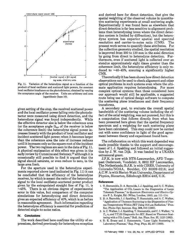
Fig. 11. Variation of the heterodyne signal as a function of the product of local oscillator and scattered light powers, for constant local oscillator irradiance on the photodetector, obtained by varying the acceptance angle of the receiver. Units are arbitrary and axes

logarithmic (base 10).

given setting of the stop, the received scattered power and the local oscillator power falling onto the photodetector were measured using direct detection, and the heterodyne signal was found independently. While the effective detector size is below the coherence area (or the acceptance angle Ωhet of the receiver is below the coherence limit) the heterodyne signal power increases linearly with the product of local oscillator and incident scattered light power; when it becomes larger than the coherence area the rate of increase reduces until it increases only as the square root of the incident power. The two regimes are seen in the data of Fig. 11. A physical explanation of this effect was given in the early review by Cummins and Swinney,20 although it is occasionally still possible to find it argued that the signal should saturate, or even reduce to zero, in the large area limit.

For the aperture used in the heterodyne experiments reported above (and indicated in Fig. 11) it can be concluded that the efficiency of the heterodyne receiver, by which is meant the ratio of the heterodyne signal to the local oscillator-scattered power product given by the extrapolated straight line of Fig. 11, is ~45%. There is an obvious degree of experimental error in this value, but comparison of the computer simulations for heterodyning and direct detection gives an expected efficiency of 40%, which is as before in reasonable agreement. Such information regarding the heterodyne efficiency is essential for prediction of detected single-to-noise ratios.

IV. Conclusions The work described here confirms the utility of ex

pressions, derived previously for heterodyne reception

and derived here for direct detection, that give the spatial weighting of the observed volume in quantitative scattering experiments at small scattering angle. Experimentally it was found here as elsewhere that direct detection is far less sensitive to alignment problems than heterodyning (even where the direct detection system is limited by diffraction), but the heterodyne system has superior spatial and spectral resolution and carrier-to-noise ratio (CNR). The present work serves to quantify these attributes. For the collection geometry studied, the spatial resolution is improved from 200 to 130 mm in the axial direction by going from direct to heterodyne detection. Furthermore, even if scattered light is collected over an etendue approximately eight times greater than the coherence limit, the heterodyne efficiency is only reduced to ~40–45%, ensuring a significantly higher CNR.

Theoretically it has been shown how direct detection observations can be used to check alignment and other optical problems in such systems even where the ultimate application requires heterodyning. For more complex optical systems than those considered here our approach would still be applicable, a suggested route being use of optical design software to compute the scattering plane irradiances and their frequency transforms.

A secondary goal, to evaluate the overall spatial bandwidth of the scattering volume including the effect of the axial weighting, was not pursued, but this is a computation that follows directly from what has been presented here given that the spatial frequency spectrum and a weighting for each scattering plane have been calculated. This step could now be carried out with some confidence in light of the good agreement between theory and experiment found here.

The collaboration on which this work depended was made possible thanks to the support and encouragement of I. J. Spalding and followed an initial suggestion by J. W. van Dijk. It was funded by a UKAEA extramural grant.

J.F.K. is now with HTS-Leeuwarden, AFD Toege-past Onderzoek, Vondelstr. 9, 8932 HP Leeuwarden, The Netherlands; B.J.R. is with CIRES, University of Colorado/NOAA, Boulder, CO 80309-0216; and A.C.W. is with Heriot-Watt University, Department of Physics, Riccarton, Edinburgh EH14 4AS, U.K.

References 1. T. Stamatakis, D. A. Reynolds, I. J. Spalding, and A. C. Walker,

"The Application of CO2 Lasers to the Diagnostics of Large Tokamak Plasmas," in Quantum Electronics and Electro-Optics P. L. Knight, Ed. (Wiley, London, 1983), pp. 111-114.

2. D. A. Reynolds, I. J. Spalding, T. Stamatakis, and A. C. Walker, "Application of Thomson Scattering to the Diagnostics of Plasma Temperatures Within JET Using 10.6 µm Radiation," Proc. Soc. Photo-Opt. Instrum. Eng. 369, 616 (1982).

3. A. C. Walker, I. J. Spalding, T. Stamatakis, and C. I. Walker, "A Te, ne and TTi(0) Diagnostic for JET, Based on Thomson Scattering with a CO2 Laser," Bull. Am. Phys. Soc. 27, 1123 (1982).

4. D. E. Evans and J. Katzenstein, "Laser Light Scattering in Laboratory Plasmas," Rep. Prog. Phys. 32, 207 (1969).


5. R. E. Slusher and C. M. Surko, "Study of Density Fluctuations in Plasmas by Small-Angle CO2 Laser Scattering," Phys. Fluids 23, 472 (1980).

6. E. Holzauer and J. H. Massig, "An Analysis of Optical Mixing in Plasma Scattering Experiments," Plasma Phys. 20, 867 (1978).

7. L. E. Sharp, A. D. Sanderson, and D. E. Evans, "Signal to Noise Requirements for Interpreting Submillimetre Laser Scattering Experiments in a Tokamak Plasma," Plasma Phys. 23, 357 (1981).

8. S. A. Ramsden, P. K. John, B. Kronast, and R. Bensch, "Evidence for a Thermonuclear Reaction in a Theta Pinch Plasma from the Scattering of a Ruby Laser Beam," Phys. Rev. Lett. 19, 688 (1967).

9. A. Thompson and M. F. Dorian, "Heterodyne Detection of Monochromatic Light Scattered from a Cloud of Moving Particles," General Dynamics Convair Division Report GDC-ERR-AN-1090, San Diego, CA (1967).

10. B. J. Rye, "Primary Aberration Contribution to Incoherent Backscatter Heterodyne Lidar Returns," Appl. Opt. 21, 839 (1982).

11. W. D. Jones, L. Z. Kennedy, J. W. Bilbro, and H. B. Jeffreys, "Coherent Focal Volume Mapping of a cw CO2 Doppler Lidar," Appl. Opt. 23, 730 (1984).

12. M. Born and E. Wolf, Principles of Optics (Pergamon, Oxford, 1964).

13. J. W. Goodman, Introduction to Fourier Optics (McGraw-Hill, New York, 1958).

14. J. F. Kusters, B. J. Rye, and A. C. Walker, "Spatial Weighting Simulations for Plasma Scattering with Heterodyne Reception," presented at U.K. Quantum Electronics Conference, Brighton (1983).

15. J. F. Kusters, B. J. Rye, and A. C. Walker, "Range Weighting for Incoherent Scattering Experiments," in Proceedings, Third International Topical Meeting on Coherent Lidar: Technology and Applications, Malvern (1985).

16. J. F. Kusters, "Spatial Weighting for Incoherent Scattering Experiments," M.Sc. Thesis, U. Hull (July 1985).

17. A. E. Siegman, "The Antenna Properties of Optical Heterodyne Receivers," Appl. Opt. 5, 1588 (1966); Proc. IEEE 54, 1350 (1966).

18. J. Harms, W. Lahmann, and C. Weitkamp, "Geometrical Compression of Lidar Return Signals," Appl. Opt. 17, 1131 (1978).

19. R. N. Bracewell, The Fourier Transform and Its Applications (McGraw-Hill, New York, 1965).

20. H. Z. Cummins and H. L. Swinney, "Light Beating Spectroscopy," Prog. Opt. 8, 123 (1970).


Spatial weighting in laboratory incoherent light scattering experiments

Documents

Transcript of Spatial weighting in laboratory incoherent light scattering experiments