arX

iv:0

901.

3478

v1 [

stat

.AP]

22

Jan

2009

The Annals of Applied Statistics

2008, Vol. 2, No. 4, 1148–1169DOI: 10.1214/08-AOAS166c© Institute of Mathematical Statistics, 2008

SPATIAL–TEMPORAL MESOSCALE MODELING OF RAINFALL

INTENSITY USING GAGE AND RADAR DATA

By Montserrat Fuentes,1 Brian Reich2 and Gyuwon Lee

North Carolina State University, North Carolina State University and

Kyungpook National University

Gridded estimated rainfall intensity values at very high spatialand temporal resolution levels are needed as main inputs for weatherprediction models to obtain accurate precipitation forecasts, and toverify the performance of precipitation forecast models. These grid-ded rainfall fields are also the main driver for hydrological modelsthat forecast flash floods, and they are essential for disaster predic-tion associated with heavy rain. Rainfall information can be obtainedfrom rain gages that provide relatively accurate estimates of the ac-tual rainfall values at point-referenced locations, but they do notcharacterize well enough the spatial and temporal structure of therainfall fields. Doppler radar data offer better spatial and temporalcoverage, but Doppler radar measures effective radar reflectivity (Ze)rather than rainfall rate (R). Thus, rainfall estimates from radar datasuffer from various uncertainties due to their measuring principle andthe conversion from Ze to R. We introduce a framework to combineradar reflectivity and gage data, by writing the different sources ofrainfall information in terms of an underlying unobservable spatialtemporal process with the true rainfall values. We use spatial logisticregression to model the probability of rain for both sources of data interms of the latent true rainfall process. We characterize the differentsources of bias and error in the gage and radar data and we estimatethe true rainfall intensity with its posterior predictive distribution,conditioning on the observed data. Our model allows for nonstation-ary and asymmetry in the spatio-temporal dependency structure ofthe rainfall process, and allows the temporal evolution of the rain-fall process to depend on the motions of rain fields, and the spatialcorrelation to depend on geographic features. We apply our methodsto estimate rainfall intensity every 10 minutes, in a subdomain overSouth Korea with a spatial resolution of 1 km by 1 km.

Received December 2007; revised February 2008.1Supported in part by NSF Grants DMS-03-53029 and DMS-07-06731.2Supported by NSF Grant DMS-03-54189G.Key words and phrases. Conditionally autoregressive models, full symmetry, nonsta-

tionarity, rainfall modelling, spatial logistic regression, spatial–temporal models.

This is an electronic reprint of the original article published by theInstitute of Mathematical Statistics in The Annals of Applied Statistics,2008, Vol. 2, No. 4, 1148–1169. This reprint differs from the original in paginationand typographic detail.

1

2 M. FUENTES, B. REICH AND G. LEE

1. Introduction. Precipitation is a key component that links the atmo-sphere, the ocean and the Earth’s surface through complex processes. Thus,accurate knowledge of precipitation levels is a fundamental requirement forimproving the prediction of weather systems and of climate change. In par-ticular, some of the weather forecast models use data assimilation techniquesthat require accurate precipitation estimates at high spatial and temporalresolutions. Accurate rain maps are also used to verify the performance ofprecipitation forecast models and can pinpoint the shortcomings of numeri-cal models. From a hydrological point of view, the rainfall is a main driverin predicting stream flow. Accurate estimated spatial and temporal struc-tures of precipitation are the most important component to understand andpredict flash flood. Rain gages are widely used to measure rainfall accu-mulation, but the information they provide is limited by their spatial andtemporal resolution. In particular, the deployment of dense rain gage net-works to resolve detailed spatial structure of rain fields is costly and theirmaintenance is time-consuming.

Remote sensing technology has improved significantly over the last fewdecades and can now provide quantitative information on precipitation.Doppler radars estimate instant rainfall intensity or rate (R) at very highspatial and temporal resolution (typically, 1 km by 1 km and in the orderof minutes). However, a radar does not measure rainfall rate directly butinfers the rain rate from the measured effective radar reflectivity (Ze). Theconversion from radar reflectivity Ze to rainfall R is usually done with thetransformation Ze= αRβ , where α = 200, β = 1.6 [e.g., Lee and Zawadzki(2005)]. This conversion function is typically derived from the measureddrop size distributions (DSDs). The DSDs vary with different microphysicaland dynamical processes. There is no unique conversion equation that sat-isfies all different processes, rather varies from storm to storm and withinstorm [e.g., Lee and Zawadzki (2005)]. The error associated with the R–Zeconversion is inherent. Thus, the main source of error of the radar rainfallestimates are associated with reflectivity measurement errors and R–Ze con-version errors. Many studies have attempted to correct for these two typesof errors [e.g., Zawadzki (1984), Joss and Waldvogel (1990), Jordan, Seedand Austin (2000), Germann et al. (2006), Lee and Zawadzki (2005), Bellonet al. (2006)].

Even when these conversion errors are corrected based on an understand-ing of the physical processes and the Ze measurement errors are reduced,the radar data are not directly comparable to rain gage measurements dueto the differences in sampling volumes between the two different sensors. Arain gage accumulates rainfall at a point on the ground, while radar sam-ples at a volume of approximately 1 km3 at some height above the ground.Rain gages are also relatively sparse across space (in relation to the spatialresolution of the radar data), thus, it is difficult to infer small scale rainfall

SPATIAL–TEMPORAL MESOSCALE MODELING OF RAINFALL INTENSITY 3

spatial patterns from gages. Ideally, one would want to combine both sourcesof rainfall data to obtain more accurate rainfall estimates. This paper in-troduces a statistical framework for combining radar reflectivity and gagemeasurements to obtain estimates of rainfall rate, taking into account thedifferent sources of error and bias in both sources of data. We also introducea sound statistical framework to estimate the R–Ze conversion equation asa spatial function. In some of the previous work [e.g., Chumchean, Seed andSharma (2004)] the relation between radar and gage data is only modeledwhen it rains, eliminating the zero-rain observations. In our framework, weuse all available data, including the zero-rain events. Furthermore, we usespatial logistic regression to model the probability of zero-rain for gage andradar data as a spatial process.

Statistical models have been developed to estimate the distribution of thelength of wet and dry periods of rainfall patterns [Green (1964), Hughesand Guttorp (1994), Sanso and Guenni (2000), Zhang and Switzer (2007)].In particular, the stochastic model introduced by Zhang and Switzer (2007)describes regional-scale, ground-observed storms by using a Boolean randomfield of rain patches. However, mesoscale instantaneous rainfall patterns arevery difficult to model using statistical or physical models, in part due tolack of real-time weather stations measuring rainfall intensity (the Koreannetwork is quite unique in this regard), and because of the spatial and tem-poral heterogeneity and the inherent variability of rainfall process at highresolution in space and time. This study is aimed to develop a statisticalmodel that can be implemented in real time for the estimation of rainfallintensity maps at high resolutions (1 km in space and 10 minutes in time).Our model treats the true unobservable rainfall intensity as a latent process,and we make inference about that process using a statistical framework thatrelates radar and gage data and other weather and geographic covariates tothe latent process.

Rainfall intensity changes rapidly across space and time, in particular,depending on the direction and intensity of the winds. Estimating com-plex spatial temporal dependency structures can be computationally de-manding, since it involves fitting models that go beyond the standard as-sumptions of stationarity and full symmetry of the geostatistical models.The assumption of stationarity and full symmetry for spatial–temporal pro-cesses offers a simplified representation of any variance–covariance matrix,and consequently, some remarkable computational benefits. Suppose that{Z(s, t) : s≡ (s1, s2, . . . , sd)

′ ∈D⊂Rd, t ∈ [0,∞)} denotes a spatial–temporal

process where s is a spatial location over a fixed domain D, Rd is a d-

dimensional Euclidean space and t indicates time. The covariance func-tion is defined as C(si − sj ; tk − tl|θ)≡ covθ{Z(si, tk),Z(sj , tl)}, where si =(si1, . . . , s

id)

′ and C is positive-definite for all θ, vector of covariance param-eters. Under the assumption of stationarity, we have C(si − sj ; tk − tl|θ)≡

4 M. FUENTES, B. REICH AND G. LEE

C(h;u|θ), where h ≡ (h1, . . . , hd)′ = si − sj and u = tk − tl. Nonstationary

models have been introduced by Sampson and Guttorp (1992), Higdon, Swalland Kern (1999), Nychka, Wikle and Royle (2002) and Fuentes (2002),among others. Another assumption of the commonly used spatial modelsis full symmetry. Under the assumption of full symmetry [Gneiting (2002)]we have C(h;u|θ) =C(h;−u|θ) =C(−h;u|θ) =C(−h;−u|θ). In the purelyspatial context, this property is also known as axial symmetry [Scaccia andMartin (2005)] or reflection symmetry [Lu and Zimmerman (2005)]. Stein(2005) introduced asymmetric models for spatial–temporal data. Park andFuentes (2008) have introduced this concept of lack symmetry in a more gen-eral context for nonstationary space–time process and they have developedasymmetric space–time models. However, these nonstationary and asym-metric models are computationally demanding. In our framework, we allowenough flexibility in the potentially nonstationary and asymmetric spatial–temporal evolution of the rainfall process using a computationally efficientapproach. We introduce a latent displacement vector that explains the echomotion of the rainfall intensity, we use motion field information to explainthis shift of the rainfall across space and time.

We apply our methods to estimate rainfall intensity at 4:20 am and4:30 am on July 12, 2006, for a domain over South Korea with a spatialresolution of 1 km by 1 km. The temporal resolution is limited by the up-date of the radar data (every 10 minutes). At each given time we have 102observations from the gage network and 10,000 radar reflectivity data points.

This paper is organized as follows. In Section 2 we describe the data.In Section 3 we introduce the statistical framework to combine radar andgage rainfall data. In Section 4 we apply our model to rainfall data in SouthKorea. We conclude in Section 5 with a discussion and some final remarks.

2. Data.

Radar data. The Korean Meteorological Administration (KMA) oper-ates 11 Doppler weather radars (4 C-band and 7 S-band) and collects radarvolume scans every ten minutes. In this study we use 10 minutes radar datafor July 12, 2006 over a subdomain in South Korea at 4:20 am and 4:30 am.The constant altitude Plan Position Indicators (CAPPI) of equivalent radarreflectivity is constructed from each volume scan at 1.5 km height and atemporal and spatial resolution of 10 minutes and 1 km, respectively, af-ter eliminating ground clutter (GC) and anomalous propagation (AP). Thereflectivity composite is produced from individual radar CAPPIs with anarray of 901 by 1051 at the spatial and temporal resolutions of 1 km and10 minutes. The weather radars at short wavelengths such as the C-band(∼5 cm) suffer from serious attenuation of signals due to strong precipita-tion over a radar or along the path of the radar beams. In addition, radar

SPATIAL–TEMPORAL MESOSCALE MODELING OF RAINFALL INTENSITY 5

measurements are limited by the blockage of radar beams by complex ter-rain over the Korean peninsula. The correction of the attenuation and beamblockage could be obtained with complex algorithms that are very compu-tationally demanding. Here, we use a standard approach and we select themaximum value at the overlapping grids to mitigate the attenuation andbeam blockage.

The radar composite in South Korea is re-sampled at the smaller domainof 100 km by 100 km around Seoul, South Korea, with latitude rangingfrom 36.977 to 37.898 and longitude ranging from 126.173 to 127.33. Thissubdomain particularly provides a dense network of rain gages (see Figure 1).There are two radar stations within this subdomain, at locations (37◦26′,126◦57′) and (37◦27′, 126◦21′) (see Figure 4). The radar on the left-handside in Figure 4 is C-band so its measurements are affected by attenuationerrors. Some of the radar data on the right upper and lower areas of oursubdomain are obtained from additional S-band KMA radars located outsideour geographic subdomain and, thus, are not shown in Figure 4.

The radar precipitation map is typically generated by converting radarequivalent reflectivity (Ze) into rainfall intensity [R, units = (mm/h)] us-ing the relationship Ze= αRβ , α is generally set to 200 and β to 1.6. Theconversion can result in some error associated with the variation of micro-physical processes. The conversion errors vary in time and space [Lee andZawadzki (2005), Lee et al. (2007)]. In this paper we work directly with thereflectivity Ze and we estimate the values of α and β, treating α as a spatialprocess.

Station data. The Korean automatic weather stations (AWS) measurethe precipitation accumulation, the east–west component of the wind vector(m/s) (u wind component), the north–south component of the wind vector(m/s) (v wind component), temperature (◦C) and relative humidity (%)every minute. The bucket size of rain gage is 0.5 mm and the number of tipsis recorded every minute from which the 1-minute rainfall intensity (mm/h)is derived using a standard approach called the Tropical Rainfall MeasuringMission (TRMM)/Gauge Data Software Package (GSP) algorithm [Wang,Fisher and Wolf (2008)]. This algorithm first identifies the rain event bychecking the time interval between two tips and fills the gap between twotips by adding a half-tip. Then, the cumulative distribution of the amount ofrain is derived as a function of time (using cubic splines) and the 1-minuterainfall intensity is obtained from the slope of this function. To minimize therandom measurement noise, a 10-minutes moving average centered at thegiven time is applied, and then the averaged values at the radar measurementtime are re-sampled. Zero values represent no-rain but they can also occurby malfunctioning gages. The obtained values are point measurements sorepresentative errors need be characterized. In this study we use the weather

6 M. FUENTES, B. REICH AND G. LEE

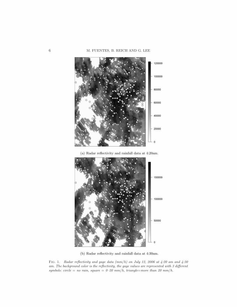
Fig. 1. Radar reflectivity and gage data (mm/h) on July 12, 2006 at 4:20 am and 4:30am. The background color is the reflectivity, the gage values are represented with 3 differentsymbols: circle = no rain, square = 0–20 mm/h, triangle=more than 20 mm/h.

SPATIAL–TEMPORAL MESOSCALE MODELING OF RAINFALL INTENSITY 7

stations over a subdomain in South Korea with latitude values ranging from

36.977 to 37.898 and longitude values from 126.173 to 127.33, for July 12,

2006. The total number of weather stations in our subdomain is 102. The

climate weather stations in the U.S. record rainfall accumulation every hour

and there are only few stations very sparse across space that record real-time

meteorological data. Some special stations transmit high temporal resolution

in real time. However, all station data used in this study are transmitted

every minute in real time. The average spatial resolution is about 13 km

and even higher around large cities (few kilometers in some parts of our

subdomain). In addition, the weather system in South Korea has complex

mesoscale features due to interactions with mountains and oceans. Thus,

these station data provide a unique opportunity to explore the small scale

structure of rain fields.

Elevation data. Geographical data are useful to understand the modu-

lation of precipitation systems by surface conditions, in particular, in Korea

where weather systems interact with complex geography. In this study we

use Digital Elevation Model (DEM) data. The DEM elevation data (in me-

ters above sea level) have resolution of 1 km and are available from the US

Geological Survey. The elevation increases as we move west-to-east in the

eastern part of our subdomain. Thus, this phenomenon could lead to more

beam blockage for the radar data in these areas, which is compensated by

selecting maximum values for the overlapping radar data.

3. Model description. Let R̂(s, t) be the continuous spatial temporal

process with the observed precipitation values at location s and time t as

measured by the rain gages, and R̃i(t) the radar reflectivity data for grid

cell i and time t. Ri(t) represents the continuous component (when it rains)

of the underlying true instant rainfall process at time t averaged within grid

cell i. We model the latent rainfall process Ri(t) in the natural logarithm

scale, and we denote Yi(t) = log(Ri(t)). The logarithm transformation is

preferred since in the original scale too much attention is given to strong

rainfall rates [Lee and Zawadzki (2005)].

In our framework we have 2 main stages. This framework is fitted using

a fully Bayesian approach. In stage 1 we model the different sources of data

in terms of an underlying latent rainfall process, and in stage 2 we describe

the model for the latent process given some weather covariates. We add a

stage 0 to model the weather covariates; this stage is implemented outside

the fully Bayesian framework for computational convenience.

8 M. FUENTES, B. REICH AND G. LEE

Stage 0.

Covariates. In our framework the weather variables, such as tempera-ture, relative humidity, and wind fields are important covariates to explainthe latent rainfall process and its temporal evolution. However, these weathercovariates are not observed at all locations of interest for rainfall predictionwithin our 1 km by 1 km resolution gridded domain. Therefore, we do spatialinterpolation using thin plate splines. The number of basis is chosen usinggeneralized cross-validation (GCV) [Craven and Wahba (1979)].

Stage 1.

Gage data model. We model the gage data in terms of an underlyingtrue rainfall process (averaged within each grid cell) with some error, andwe model the probability of zero-rain for the gage data as a spatial processπg(s, t) also in terms of the latent rainfall process. We call this model azero-inflated log-Gaussian process (LGP). Thus, we have

R̂(s, t) =

{

0, πg(s, t),

exp{Yi(s)(t) + ǫg(s, t)}, 1− πg(s, t),

with πg(s, t) the probability of zero rain at location s and time t for the raingage data. The subindex i(s) for the process Y with the log rainfall valuesrefers to the grid cell containing s. The component ǫg(s, t) characterizesthe variations in the gage data with respect to the truth at location s andtime t, due to measurement error and also due in part to the temporal andspatial misalignment (different scales) of the gage data and the truth. Themisalignment is a consequence of the temporal averaging of the gage datato obtain R̂(s, t) and the spatial averaging of the truth. This variation isexpected to be proportional to the precipitation levels that is why we havemultiplicative errors in the original scale.

The logits of the unknown π(s, t) probabilities (i.e., the logarithms ofthe odds) are modeled as a linear function of the rainfall values (log scale)Yi(s)(t), using a spatial logistic regression model,

logit(πg(s, t)) = ag + bgYi(s)(t),

where ag and bg are unknown coefficients.In our zero-inflated LGP we model the probability of zero rain in terms

of the continuous component of the rainfall, Yi(s)(t), and thus, it differsfrom most zero-inflated models that treat the probability of zero and thecontinuous part independently. This is an important feature of our modelthat allows to smooth some unrealistic nonzero values (due to measurementerror) in the middle of a storm.

SPATIAL–TEMPORAL MESOSCALE MODELING OF RAINFALL INTENSITY 9

Radar reflectivity model. For the radar reflectivity data we have a simi-lar model, except for the fact that we add multiplicative and additive biascomponents to the reflectivity–rainfall conversion model,

R̃i(t) =

{

0, πr(i, t),

exp{c1(i) + c2Yi(t) + ǫr(i, t)}, 1− πr(i, t),

with πr(i, t) the probability of zero-rain for the radar data at time t andgrid cell i. The above relationship [when R̃i(t)> 0] is the reflectivity–rainfallconversion function,

log(R̃i(t)) = c1(i) + c2 log(Ri(t)) + ǫr(i, t),

with the parameter c1 a spatial function (additive bias term), c2 a multi-plicative bias term and ǫr a random error component. We tried to modelthe parameter c2 as a spatial function too, but that led to a lack of iden-tifiability problem. The reflectivity–rainfall conversion function is modeledin the natural logarithm scale, because the error component is thought toincrease with the precipitation values, and in the original scale too muchweight is given to high rainfall rates [Lee and Zawadzki (2005), Germannand Zawadzki (2002)]. The logits of the unknown πr(i, t) probabilities aremodeled as a linear function of the Yi(t),

logit(πr(i, t)) = ar + brYi(t),

where ar and br are unknown coefficients. Modeling the probability of zerorain in terms of the rainfall continuous component becomes very relevant forthe radar measurements, since in many occasions we obtain isolated zero-rain events due to radar measurement error in the middle of a storm (seezero-rain radar data in the middle of our geographic domain in Figure 1).

Stage 2.

Latent rainfall process. The latent rainfall process (log scale) Yi(t) ismodeled as a spatio-temporal Gaussian Markov random field. The pro-cess at the first time point Y(1) = (Y1(t), . . . , Yn(t))

′ has a conditionallyautoregressive prior (CAR) prior. The CAR prior for Y(1) is a multivari-ate normal with a mean X(1)β, for X(1) = (X1(1), . . . ,Xn(1))

′, that is alinear function of temperature, relative humidity and elevation at time 1,and with inverse covariance τ2YQY , where τ

2Y ∼Gamma(0.5,0.005) is an un-

known precision, and QY = (I − ρY DW ), where ρY ∈ (0,1), I is a diagonalmatrix with Iii = 1, Wik = wik ≥ 0 for i 6= k and Wii = wi+ =

∑

k 6=iWik,and D =Diag(1/wi+) is a diagonal matrix with Dii = 1/wi+. An attractivefeature of this prior is that the full conditional prior Yi(1)|Yk(1), k 6= i, isnormal with mean ρY (

∑

k 6=iwik

wi+(Yk(1) +Xi(1)β)) and variance 1/(τ2wi+).

We assume the weights wjk are known and equal to wjk = I(j ∼ k), whereI(j ∼ k) indicates whether cells j and k are adjacent.

10 M. FUENTES, B. REICH AND G. LEE

Temporal evolution of the latent rainfall process. Successive values ofYi(t) are modeled using a dynamic linear model [Gelfand, Banerjee andGamerman (2005)]. The usual dynamic linear model smoothes Yj(t) towardthe cell j’s previous value, Yj(t− 1), that is,

Yi(t) = ρYi(t− 1) +Xi(t)β + ǫi(t),(1)

where ρ ∈ (0,1) controls the amount of temporal smoothing, ǫi(t) is a multi-variate normal vector with CAR prior, and with inverse covariance τ2ǫ(t)Qǫ(t)

[similar to the CAR model for Y(1), but with mean zero], Xi is a vectorwith the following covariates: elevation and the temporal gradients of tem-perature and relative humidity. However, this is inappropriate for rain databecause the storm moves over time. To correctly model the storm dynamics,we introduce a displacement vector ∆i(t) that explains the echo motion atthe grid point i. The model then becomes

Yi(t) = ρYi+∆i(t)(t− 1) +Xi(t)β + ǫi(t),(2)

if the shift ∆ at a given time is not a function of space that would imposeone constant translation vector, and it would not allow for rotation. To allowenough flexibility in the temporal evolution of the rainfall process, we model∆ as a spatial categorical process and we use the wind field information (uand v components) (Figure 2) as relevant covariates to explain the shift. Wewrite Wu,i(t) and Wv,i(t) to denote the u and v components of the windat time t and location i. S(t) represents a spatial spline basis function attime t [number of basis components is chosen using DIC (deviance informa-tion criterion), Speigelhalter et al. (2002)] at time t, and α, β1 and β2 areunknown coefficients. The basis function for S(t) are the tensor product oftwo 1-dimensional cubic B-spline basis functions. This type of basis func-tions was chosen for computational convenience, while still providing enoughsmoothing for the term S(t). We used information criteria for the selectionof number of basis and we ran sensitivity analysis.

We have

∆i(t) = ([δ1,i(t)], [δ2,i(t)]),

where [x] rounds to the nearest integer to x, and

δ1,i(t) = αWu,i(t) + S(t)β1

and

δ2,i(t) = αWv,i(t) + S(t)β1.

We introduce a spline basis function to characterize the behavior of thestorm motion not explained by the wind fields. The wind fields (Figure 2)can be very noisy at this high spatial–temporal resolution, so additionalsmoothing is needed and that is the role of the spline basis functions.

SPATIAL–TEMPORAL MESOSCALE MODELING OF RAINFALL INTENSITY11

Fig. 2. Wind fields on July 12, 2006 at 4:20 am. The arrow points in the direction thewind is moving toward and the length of the stem of the arrow is proportional to windspeed.

We estimate the rainfall intensity, Ri(t), and the probabilities of zero-rainfor the gage and radar data, πg(s, t) and πr(i, t), with their predictive pos-terior distribution summaries. We fit this framework using a fully Bayesianapproach. MCMC sampling is carried out using the software R [R Devel-opment Core Team (2006)]. Metropolis sampling is used for all parameters.The standard deviations of the Gaussian candidates are tuned to give accep-tance probabilities near 0.40. Convergence is monitored by inspecting traceplots of the deviance and several representative model parameters.

3.1. Covariance function of the rainfall intensity. It is of interest to cal-culate the spatial–temporal covariance of the latent rainfall process, as ameasure of the dependency structure and variability across time and spaceof the true underlying rainfall process. The process Y(1) has inverse co-variance τ2Y QY (defined in the previous section). Conditioning on the shiftvector, the covariance of Y (log of the rainfall intensity) is

cov(Yi(t), Yi+h(t+ τ))

12 M. FUENTES, B. REICH AND G. LEE

= ρ2t+τ τ−2Y Q

(−1)Y

(

i+t∑

k=2

∆i1k

(k); i+ ht+τ∑

k′=2

∆i2k′(k′)

)

+t∑

j=2

ρ2t−2j+2+τ τ−2ǫ(j−1)Q

(−1)ǫ(j−1)

(

i+t∑

k=j

∆i1k

(k); i+ h+t+τ∑

k′=j

∆i2k′(k′)

)

+ ρττ−2ǫ(t)Q

(−1)ǫ(t)

(

i; i+ h+t+τ∑

k′=t+1

∆i2k′(k′)

)

,

where ρ is the smoothing parameter used in equation (2), Q(−1)(i, j) denotesthe (i, j) element (row i, column j) of the inverse matrix of Q, and thesubindexes i2k and i1k for ∆(k) are functions of the location i and values of∆ at other time points than k. When the shift is constant across space, thecovariance above becomes a mixture of CAR covariance models. However,by allowing the shift to change across space depending on the wind fieldsand geographic features, the covariance becomes space-dependent and showsdifferent patterns across space (nonstationarity).

Thus, by using latent processes, we allow the spatial dependency of thelog instant rainfall process, Yi, to depend on location, rather than just beingmodeled as a function of distances between grid cells (stationarity assump-tion). From the previous expression for the covariance of the process Yi, wesee that the temporal evolution of the rainfall process at different locationsis a function of the shift vector with the wind fields, allowing for the lack offull symmetry in the space–time covariance.

4. Application. The relatively dense spatial coverage of the Korean au-tomatic weather stations with 1-minute weather measurements, combinedwith the high spatial resolution of the Doppler radar data from KMA, pro-vide a unique opportunity to study the radar reflectivity–rainfall conversionfunction, and to develop frameworks for spatial temporal mesoscale mod-eling of rainfall intensity. Lee, Seed and Zawadzki (2007) modeled the spa-tial/temporal variability of the conversion errors by using reflectivity andrainfall rate measurements at a fixed location. In the work by Lee, Seedand Zawadzki (2007) the conversion errors were not modeled across spaceand time due to the limited observations. In the work presented here weintroduce a statistical model that can capture the complex and heteroge-neous spatial temporal structure of mesoscale rainfall intensity combininggage and radar reflectivity data with a resolution of 10 minutes (time) and1 km ×1 km (space). Figure 1(a) presents the radar reflectivity (Ze) andgage rainfall rate (R in mm/h) on July 12, 2006 at 4:20 am. The empiricalPearson correlation between log radar reflectivity and log gage data is 0.5.There is an overall agreement between both sources of information in terms

SPATIAL–TEMPORAL MESOSCALE MODELING OF RAINFALL INTENSITY13

Table 1We present the DIC value, the posterior expectation of the deviance (D̄) and the

estimated effective number of parameters pD, for 5 different models. Model 1: shift andbias constant across space. Model 2: shift varying spatially and bias constant across

space. Model 3: shift constant across space and bias varying spatially. Model 4: shift andbias varying spatially (9 spline basis components). Model 5: shift and bias varying

spatially (25 spline basis components)

Model DIC D̄ pD

1 18700 13092 56072 18223 12535 56883 19247 13377 58704 17722 12020 57025 18813 12436 6377

of capturing the large scale structure. However, there are discrepancies atsome given locations. Similar empirical correlations are obtained at othertime points.

Figure 1(b) presents both sources of information on July 12, 2006 at4:30 am (the next time point). There is a storm moving from the south-western to the north-eastern part of our domain, and both sources of dataseem to capture that phenomenon, showing, however, small scale disagree-ments in the intensity of the rainfall. We use the statistical framework intro-duced in this paper to combine radar reflectivity and gage data to estimaterainfall intensity.

To determine and justify the need of the more complex model proposedin this paper, in which we introduce a spatially varying bias function (c1),and a spatially varying shift vector (∆), we compare 5 different models thatassume different spatial structure for the additive bias and the shift vector.In Model 1 we present a simple model, where the shift and bias are constantfunctions across space. In Model 2 the shift is varying spatially (using themodel in Section 3) and the additive bias is constant across space. In Model 3the shift is constant across space and the bias is varying spatially. In Model 4the shift and bias are varying spatially this is the general model presented inSection 3, using 9 basis components for the cubic B-spline function (tensorproduct of two 1-dimensional cubic B-spline basis functions). Model 5 isthe same as Model 4 but with a different number of components for thespline function (25 basis components). In Table 1 we present some modelcomparisons.

We use the DIC [deviance information criterion, Speigelhalter et al. (2002)]to compare model performance. PD indicates the estimated effective num-ber of parameters. Model 3 has larger PD than Model 4, even if Model 4is a more complicated model. The reason for that is that Model 4 has a

14 M. FUENTES, B. REICH AND G. LEE

spatially-varying shift, while Model 3 does not, and adding a small numberof shift parameters aligns the two time points in a way that allows for moretemporal smoothing and thus fewer effective random effects. Model 4 hasthe smallest DIC, and we give next a summary of the results for that model.

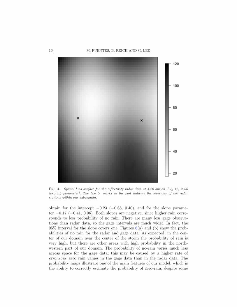
The prior used for the multiplicative bias (parameter c2 in the reflectivity–rainfall conversion equation) is a Gamma(1,1). The posterior median (95%interval) for this multiplicative bias is 1.05 (1.08, 1.13), which seems to in-dicate that the recommended 1.6 value for the multiplicative bias (obtainedbased on regression analysis) might not be always appropriate. In Figure 3we plot the rainfall gage data versus the reflectivity radar data for our sub-domain on July 12,2006 at 4:20 am and 4:30 am, eliminating the no-rainevents; we also show the standard conversion curve (Ze = 200R1.6). Theplot of the spatial posterior median for the spatial bias [parameter exp(c1)]is presented in Figure 4. The bias is larger in the south-eastern part of oursubdomain, where there seems to be more disagreement between radar andgage data. This figure also shows the location of the two radar stations.There is not much relationship between the location of the radar stationsand the magnitude of bias for the radar data. It is true that as the radarbeams propagate through the range of coverage of the Doppler radar, thesampling volume and measurement heights increase. In addition, at largerdistances from the station the radar beams can intercept the melting layerof the stratiform rain. Intercepting the melting layer could result in high val-ues of radar reflectivity, mainly due to the increase of the dielectric constantwhile maintaining the size of the individual precipitation particles. This phe-nomenon could increase the radar bias at locations that are further awayfrom the station. However, the current storm is mostly a convective system,where the increase of reflectivity in the melting layer is less significant orit is not present. Thus, a larger bias is not expected further away from theradar stations.

The estimated values of c2 were very similar for the other 4 models, whichseems to indicate that this parameter is robust to the structure imposed onthe additive bias and the shift parameter. The number of basis componentsfor the spline surface is 9 for both the additive bias and also for the shiftvector. Models with a different number of spline basis components had higherDIC values (see, e.g., Model 5).

We present in Figure 5 the vector that shows the storm motions (∆i(t)).The values presented are the mean of the posterior distribution of the stormdirection. We can appreciate in this graph the flexibility offered by our sta-tistical framework to characterize nonstationary and complex patterns inthis motion. The estimated displacement vector shows the dominant south–west to north–east direction of the storm, but it also captures some smallscales phenomena, such as the west–east shift in the lower left corner of ourdomain. The average shift is about 11 m/s. The median (95% interval) for

SPATIAL–TEMPORAL MESOSCALE MODELING OF RAINFALL INTENSITY15

Fig. 3. Plot of the rainfall data from rain gages, versus radar reflectivity, eliminatingthe zero-rain events, and using data from July 12, 2006 at 4:20 am and 4:30 am. Thesolid curve corresponds to the standard transformation Ze = 200R1.6. This scatterplot isgenerated in the natural logarithmic scale for both variables (log of rainfall versus log ofreflectivity), presenting the reflectivity radar and gage data on the original scale on theaxes.

the coefficient α that measures the effect of the smoothed wind fields onthe shift is 0.39 (0.22, 0.55), which indicates that the smoothed wind playsan important role explaining the storm motion (Figure 5). This might beexpected, since storm systems move along the wind fields at steering levels(around 700 to 500 hPa). However, it is also true that the surface winds(Figure 2) are highly affected by local effects such as terrain and local heat-ing. On the other hand, the smoothed version of the wind fields used in thisapplication should attenuate the impact of those local phenomena, and bea better predictor of the shift.

It is also of interest to study the probability of rain for both gage andradar data. We used vague normal prior distributions for the logistic pa-rameters, N(0,1/0.01), where 0.01 is the precision. The median (95% in-tervals) for the logistic parameters that explain the probability of zero-rainfor the radar data are −2.81 (−3.08, −2.61) for the intercept parameter,and −1.69 (−1.83, −1.58) for the slope parameter. For the gage data, we

16 M. FUENTES, B. REICH AND G. LEE

Fig. 4. Spatial bias surface for the reflectivity radar data at 4.20 am on July 12, 2006[exp(c1) parameter]. The two × marks in the plot indicate the locations of the radarstations within our subdomain.

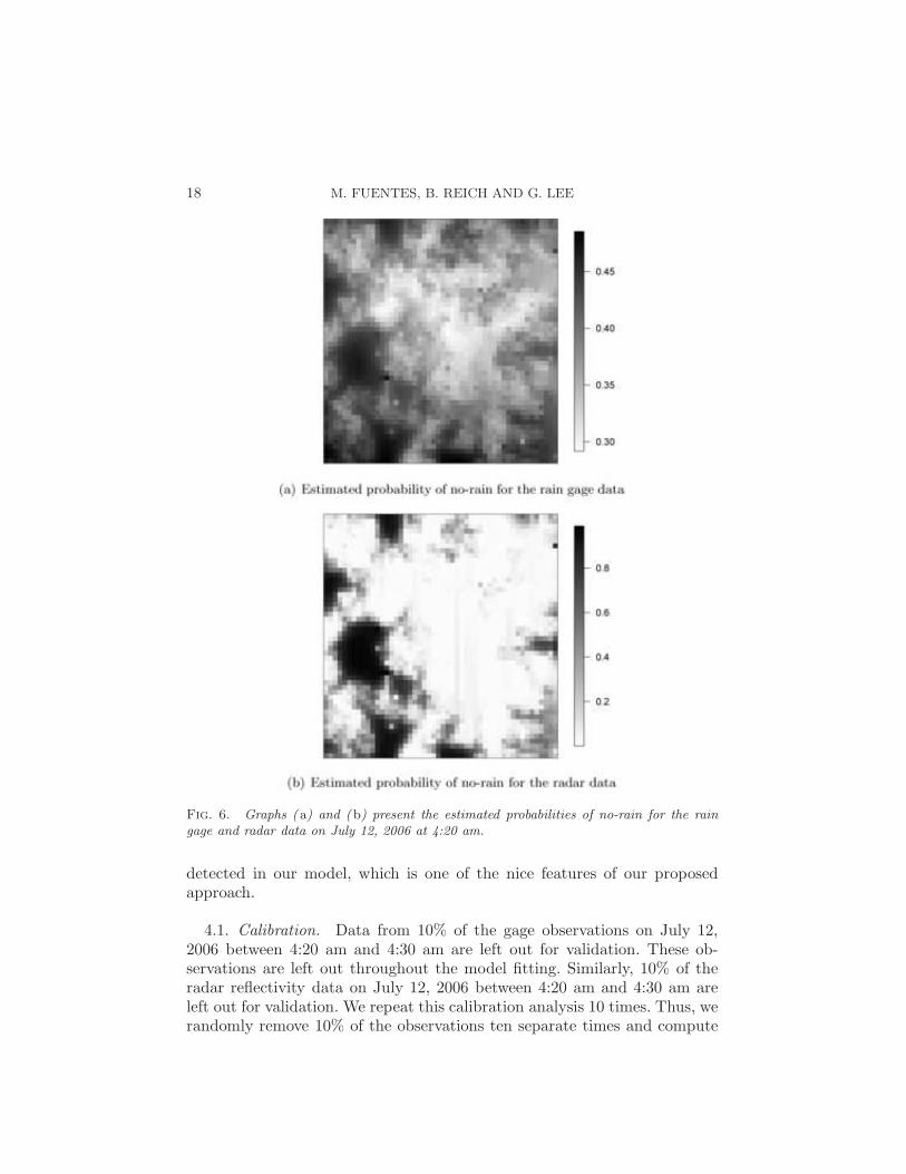
obtain for the intercept −0.23 (−0.68, 0.40), and for the slope parame-ter −0.17 (−0.41, 0.06). Both slopes are negative, since higher rain corre-sponds to less probability of no rain. There are many less gage observa-tions than radar data, so the gage intervals are much wider. In fact, the95% interval for the slope covers one. Figures 6(a) and (b) show the prob-abilities of no rain for the radar and gage data. As expected, in the cen-ter of our domain near the center of the storm the probability of rain isvery high, but there are other areas with high probability in the north-western part of our domain. The probability of no-rain varies much lessacross space for the gage data; this may be caused by a higher rate oferroneous zero rain values in the gage data than in the radar data. Theprobability maps illustrate one of the main features of our model, which isthe ability to correctly estimate the probability of zero-rain, despite some

SPATIAL–TEMPORAL MESOSCALE MODELING OF RAINFALL INTENSITY17

Fig. 5. The mean of the posterior distribution of the shift vector on July 12, 2006 at4:30 am.

incorrect zero-rain measurements in radar and gage data in the middle ofthe storm.

We present our rainfall maps in Figures 7(a) and (b). These figures presentthe mean of the predictive posterior distribution (ppd) of the rainfall inten-sity, Zi(t), on July 12, 2006 at 4:20 am and at 4:30 am, respectively. Thesegraphs, overall, present smoother surfaces but with similar rain patterns asthe radar reflectivity images (Figure 1), except for the areas with larger bias(see bias function in Figure 4). However, the scale is different, the estimatedreflectivity–rainfall function provides the change of scale equation.

We redid the analysis setting the gage values that were thought to beerroneous as missing rather than zero, which is the default value assigned bythe recording instrumentation at the gages. An empirical standard approachwas used to identify erroneous gage values based on ad-hoc comparison of thegage data with the 9 closest radar pixels. When the number of nonzero rain-value pixels was greater or equal than 3, then the zero-rain gage value wasreplaced with a missing label. The obtained additive bias, shift vectors, andpredictive rainfall values [see Figure 7(c) and (d)] were very similar to theones obtained using the potentially erroneous values. This is due to the factthat in our model we characterize the uncertainty in the gage measurements,and we combine radar and gage data, so clear erroneous values should be

18 M. FUENTES, B. REICH AND G. LEE

Fig. 6. Graphs ( a) and (b) present the estimated probabilities of no-rain for the raingage and radar data on July 12, 2006 at 4:20 am.

detected in our model, which is one of the nice features of our proposedapproach.

4.1. Calibration. Data from 10% of the gage observations on July 12,2006 between 4:20 am and 4:30 am are left out for validation. These ob-servations are left out throughout the model fitting. Similarly, 10% of theradar reflectivity data on July 12, 2006 between 4:20 am and 4:30 am areleft out for validation. We repeat this calibration analysis 10 times. Thus, werandomly remove 10% of the observations ten separate times and compute

SPATIAL–TEMPORAL MESOSCALE MODELING OF RAINFALL INTENSITY19

Fig. 7. Graphs ( a) and (b) present the mean of the predictive posterior distributionof the rainfall intensity (mm/h) on July 12, 2006 at 4:20 am and 4:30 am, respectively.Graphs ( c) and (d) also present the mean of the predictive posterior distribution of therainfall intensity (mm/h) on July 12, 2006 at 4:20 am and 4:30 am, but, treating whatwere thought to be erroneous zero-rain gage values as missing rather than zero.

the coverage probabilities of the 95% prediction intervals for each of the tenanalyses.

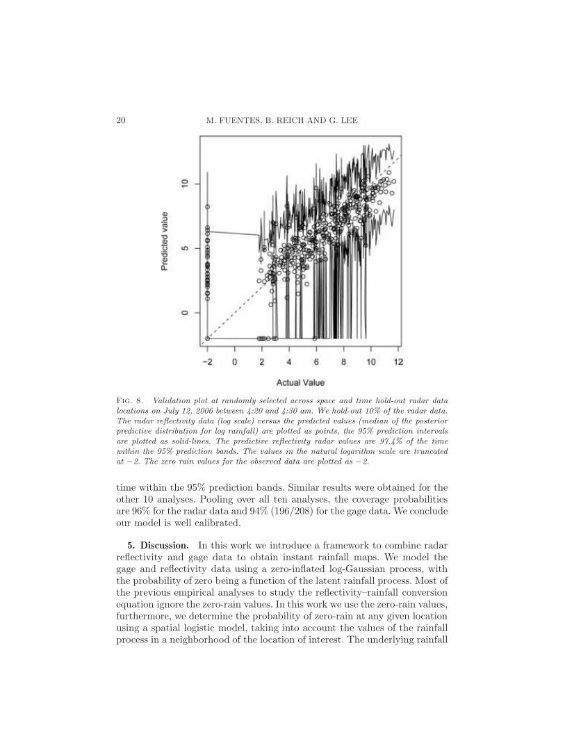
Figure 8 shows the validation plot for the radar data, for one of the 10analyses conducted. The predictive reflectivity radar values are 97.4% of the

20 M. FUENTES, B. REICH AND G. LEE

Fig. 8. Validation plot at randomly selected across space and time hold-out radar datalocations on July 12, 2006 between 4:20 and 4:30 am. We hold-out 10% of the radar data.The radar reflectivity data (log scale) versus the predicted values (median of the posteriorpredictive distribution for log rainfall) are plotted as points, the 95% prediction intervalsare plotted as solid-lines. The predictive reflectivity radar values are 97.4% of the timewithin the 95% prediction bands. The values in the natural logarithm scale are truncatedat −2. The zero rain values for the observed data are plotted as −2.

time within the 95% prediction bands. Similar results were obtained for theother 10 analyses. Pooling over all ten analyses, the coverage probabilitiesare 96% for the radar data and 94% (196/208) for the gage data. We concludeour model is well calibrated.

5. Discussion. In this work we introduce a framework to combine radarreflectivity and gage data to obtain instant rainfall maps. We model thegage and reflectivity data using a zero-inflated log-Gaussian process, withthe probability of zero being a function of the latent rainfall process. Most ofthe previous empirical analyses to study the reflectivity–rainfall conversionequation ignore the zero-rain values. In this work we use the zero-rain values,furthermore, we determine the probability of zero-rain at any given locationusing a spatial logistic model, taking into account the values of the rainfallprocess in a neighborhood of the location of interest. The underlying rainfall

SPATIAL–TEMPORAL MESOSCALE MODELING OF RAINFALL INTENSITY21

process has a nonstationary and asymmetric covariance that explains thespatial temporal complex dependency structures.

The dataset used for our analysis seem to indicate that the standard val-ues of the parameters in the reflectivity–rainfall conversion equation mightnot be appropriate for every storm and geographic domain, and that thereis need to allow the additive bias to change across space. The main differ-ences between the approach presented here and previous analyses are thetreatment of the zero values, the characterization of the storm motions, andthe fact that the additive bias is allowed to change across space. Our modelcomparisons seem to indicate that these are all important features that leadto a better and more accurate rainfall estimated surfaces.

In this paper we have made an effort to deal with the various problems ofthe rainfall data sources, but there is always more that could be done. Wediscuss here some forward-looking issues to illustrate some of the challengesin making the best use of these data. In our modeling framework we havetried to characterize the uncertainty in radar and gage data and in the R–Ze conversion equation. However, it would be helpful to conduct differentsub-analysis to study and understand better the different sources of errorthat contribute to the overall uncertainty, in particular, regarding radar mis-calibration and attenuation errors, and errors in the R–Ze conversion due tomicrophysical processes. Radar mis-calibration errors tend to provide a con-stant bias within the radar coverage range, while errors due to attenuationshow high correlation along the path, so it could be possible to separate bothsources of error. In addition, R–Ze conversion errors should be a functionof different microphysical processes. Thus, a new formulation that separatesthese various errors merits a new exploration. This would provide a betterunderstanding of error sources and a way of mitigating them.

The understanding of error structures and its use in hydrological and me-teorological models have enormous potential. Obvious applications are itsuse in probabilistic verification of the precipitation forecast from numericalmodels, and of the precipitation estimates from various remote sensing in-struments such as the space-based radiometers. From our analysis we canobtain probability maps of exceeding a certain threshold. This informationcould be used to improve the prediction of the stream flow of extreme hy-drological events, and that would aid in the preparation for extreme events.We have shown here the mean of the predictive posterior distributions whichshows a central tendency of each predictive field. Numerous predictive fieldscan be simulated from that distribution and could be used as inputs to gen-erate a hydrological and meteorological ensemble forecast. Since hydrologicaland meteorological models are nonlinear, the response to the small variationof initial inputs is highly unpredictable. Thus, an ensemble forecast basedon some initial predictive fields (as obtained in this paper) that characterizethe rainfall variability is essential to characterize extreme events.

22 M. FUENTES, B. REICH AND G. LEE

Acknowledgments. The authors greatly appreciate the Korean Meteoro-logical Administration, in particular, Dr. HyoKyung Kim and Mr. KyungYeupNam for providing the radar and surface station data. The National Centerfor Atmospheric Research is sponsored by the National Science Foundation.

REFERENCES

Bellon, A., Lee, G. W., Kilambi, A. and Zawadzki, I. (2006). Real-time comparisonsof VPR-corrected daily rainfall estimates with a gauge mesonet. J. Appl. MeteorologyClimatology 46 726–741.

Chumchean, S., Seed, A. and Sharma, A. (2004). Application of scaling in radar re-flectivity for correcting range-dependent bias in climatological radar rainfall estimates.J. Atmospheric Oceanic Technology 21 1545–1556.

Craven, P. and Wahba, G. (1979). Smoothing noisy data with spline functions: Esti-mating the correct degree of smoothing by the method of generalized cross-validation.Numer. Math. 31 377–403. MR0516581

Fuentes, M. (2002). Periodogram and other spectral methods for nonstationary spatialprocesses. Biometrika 89 197–210. MR1888368

Gelfand, A. E., Banerjee, S. and Gamerman, D. (2005). Spatial process modellingfor univariate and multivariate dynamic spatial data. Environmetrics 16 465–479.MR2147537

Germann, U., Galli, G., Boscacci, M. and Bolliger, M. (2006). Radar precipitationmeasurement in a mountainous region. Quarterly J. Roy. Meteorology Society 132 1669–1692.

Germann, U. and Zawadzki, I. (2002). Scale-dependence of the predictability of precip-itation from continental radar images. Part I: Description of the methodology. MonthlyWeather Review 130 2859–2873.

Gneiting, T. (2002). Nonseparable, stationary covariance functions for space–time data.J. Amer. Statist. Assoc. 97 590–600. MR1941475

Green, J. R. (1964). A model for rainfall occurrence. J. Roy. Statist. Soc. Ser. B 26

345–353. MR0171366Higdon, D., Swall, J. and Kern, J. (1999). Non-stationary spatial modeling. In

Bayesian Statistics 6 (J. M. Bernardo et al., eds.) 761–768. Oxford Univ. Press.Hughes, J. P. and Guttorp, P. (1994). Incorporating spatial dependence and atmo-

spheric data in a model of precipitation. American Meteorological Society 33 1503–1515.Jordan, P. W., Seed, A. W. and Austin, G. L. (2000). Sampling errors in radar

estimates rainfall. J. Geophysical Research 105 2247–2257.Joss, J. and Waldvogel, A. (1990). Precipitation measurement and hydrology. Radar

in Meteorology. In American Meteorological Society (D. Atlas, ed.) 577–606.Lee, G. W. and Zawadzki, I. (2005). Variability of drop size distributions: Time scale

dependence of the variability and its effects on rain estimation. J. Appl. Meteorology44 241–255.

Lee, G. W., Seed, A. W. and Zawadzki, I. (2007). Modeling the variability of drop sizedistributions in space and time. J. Appl. Meteorology and Climatology 46 742–756.

Lu, N. and Zimmerman, D. L. (2005). Testing for directional symmetry in spatial de-pendence using the periodogram. J. Statist. Plann. Inference 129 369–385. MR2126855

Nychka, D., Wikle, C. K. and Royle, J. A. (2002). Multiresolution models for non-stationary spatial covariance functions. Stat. Modell. 2 315–331. MR1951588

Park, M. S. and Fuentes, M. (2008). Testing lack of symmetry in spatial–temporalprocesses. J. Statist. Plann. Inference. To appear.

SPATIAL–TEMPORAL MESOSCALE MODELING OF RAINFALL INTENSITY23

R Development Core Team (2006). R: A language and environment for statisticalcomputing. Available at http://www.R-project.org.

Sanso, B. and Guenni, L. (2000). A nonstationary multisite model for rainfall. J. Amer.Statist. Assoc. 95 1089–1100. MR1821717

Sampson, P. D. and Guttorp, P. (1992). Nonparametric estimation of nonstationaryspatial covariance structure. J. Amer. Statist. Assoc. 87 108–119.

Scaccia, L. and Martin, R. J. (2005). Testing axial symmetry in separability in latticeprocesses. J. Statist. Plann. Inference 131 19–39. MR2136004

Spiegelhalter, D. J., Best, N. G., Carlin, B. P. and van der Linde, A. (2002).Bayesian measures of model complexity and fit (with discussion). J. Roy. Statist. Soc.Ser. B 64 583–639. MR1979380

Stein, M. L. (2005). Space–time covariance functions. J. Amer. Statist. Assoc. 100 310–321. MR2156840

Wang, J., Fisher, B. L. and Wolf, D. B. (2008). Estimating rain rates from tipping-bucket rain gauge measurements. J. Atmospheric and Oceanic Technology. To appear.

Zawadzki, I. (1984). Factors affecting the precision of radar measurements of rain. In 22ndConference on Radar Meteorology, Zurich. American Meteorological Society 251–256.

Zhang, Z. and Switzer, P. (2007). Stochastic space–time regional rainfall model-ing adapted to historical rain gauge data. Water Resources Research 43 W03441.DOI:10.1029/2005WR004654.

M. FuentesB. ReichDepartment of StatisticsNorth Carolina State UniversityRaleigh, North Carolina 27695USAE-mail: fuentes@stat.ncsu.edu

reich@stat.ncsu.edu

G. LeeDepartment of Astronomy and

Atmospheric SciencesKyungpook National University1370 Sangyeok-dongBukgu, Daegu, 702-701Korea (ROK)E-mail: gyuwon@knu.ac.kr