Spatial Structural Change and Agricultural Productivity∗

Fabian Eckert† Michael Peters‡

September 2017

Abstract

Standard models of structural change predict that the share of agricultural value added and agricultural

employment are equalized. In the data they are not. While both decline as the economy develops,

value added per worker in agriculture is substantially lower than in non-agriculture. Moreover, this

agricultural productivity gap is remarkably persistent despite the large reallocation of production fac-

tors across sectors. In this paper, we argue that this sectoral productivity gap might to a large extent

be a spatial gap. Using a novel dataset for more than 700 US commuting zones between 1880 and

2000, we document that agricultural employment shares are strongly negatively correlated with av-

erage earnings and uncorrelated with subsequent net population outflows. These facts are consistent

of substantive frictions to spatial mobility, which prevent the spatial equalization of marginal prod-

ucts. To quantify the strength of this mechanism, we construct a novel theory of spatial structural

change by embedding an economic geography model in a dynamic, neoclassical model of the struc-

tural transformation. We show that spatial frictions can account for more than 50% of the observed

productivity gap. This implies that the direct productivity gains from reallocating workers across

sectors are modest.

∗We thank seminar participants at Stanford, Penn State, the SED, the EEA, the NBER Macroeconomic Across Time andSpace Conference, the Edinburgh Workshop on Agricultural Productivity and the Yale International Lunch for very helpfulcomments. We are particularly thankful to Simon Alder, Timo Boppart, David Lagakos and Doug Gollin for their suggestions.We also thank Costas Arkolakis, Pete Klenow, and Aleh Tsyvinski for their comments. Zara Contractor, Andrés Gvirtz andAdam Harris provided outstanding research assistance.†Yale University. fabian.eckert@yale.edu‡Yale University and NBER. m.peters@yale.edu

1 Introduction

Standard models of the process of structural change imply that sectoral employment shares and sectoralvalue added shares are equalized. In the data they are not. Not only do agricultural employment sharesconsistently exceed the share of agricultural value added, but this “agricultural productivity gap” staysstubbornly high as countries undergo the structural transformation. A case in the point is the historicalexperience of the US. While the employment shares declined from 60% to essentially nil since 1850,value added per worker in the non-agricultural sector is about twice as high as its counterpart in theagricultural sector and varies little over time. Taken at face value, this implies that over the last 120 yearsof US growth, the marginal product of agricultural workers is about half as high as the marginal productin non-agriculture - despite the fact that more than 50% of the workforce reallocates.

In this paper, we argue that the spatial allocation of economic activity goes a long way to quantitativelyexplaining this pattern. Our argument is simple: If regions differ in their comparative advantage, indi-viduals need to relocate as the economy develops and aggregate spendings shifts away from agriculture.If mobility is costly, the process of structural change puts downward pressure on wages in rural regions,which specialize in agriculture. Both the size and the persistence of these wage differences across loca-tions depend on the speed of spatial reallocation. If spatial reallocation is subject to frictions, wage gapsemerge. Moreover, if the process of structural change evolves slowly, such wage gaps persist. In theaggregate, this spatial productivity gap manifests itself as an agricultural productivity gap, even thoughthe marginal product of labor might be equalized across sectors within a location at each point in time.

Two empirical regularities from the US experience are suggestive that this mechanism might be impor-tant. First of all, using a novel dataset on historical employment patters and manufacturing earningsacross all US counties starting in 1880, we document a sizable spatial wag gap across locations. Impor-tantly, there is a strong negative correlation with the share of agricultural employment and this correlationremains very stable between 1880 and 2000. Hence, regions specializing in agriculture are and remainlow wage regions. Our second fact suggests why such wage differentials are not arbitraged away throughspatial mobility: empirically, the extent of net migration is only weakly correlated with agricultural spe-cialization. While gross flows are substantial, the agricultural employment share is not the dominantpredictor of the direction of net flows. We for example show that the reallocation of workers from highto low agricultural places during the 20th century has essentially zero explanatory power for the declinein the aggregate agricultural employment share. This implies that the entirety of the structural transfor-mation is a within-region phenomenon and there might be very limited arbitrage (and hence aggregatereallocation gains) at the relevant, i.e. spatial, margin.

To quantify the importance of this mechanism, we combine an economic geography model with intra-national trade and labor mobility and an otherwise standard, neoclassical model of structural change.As far as the process of structural change is concerned, we follow the macroeconomic literature andallow for demand side forces (i.e. non-homothetic preferences) and supply side forces (i.e. non-balancedtechnological progress across sectors). To generate a need for spatial reallocation, we assume that regions

1

differ in their sectoral comparative advantage and workers can reallocate spatially subject to movingcosts. In order to expand, regions need to pay higher wages to attract individuals. Because the process ofstructural change requires non-agricultural intensive regions to grow, marginal products across space arenot equalized and agricultural value added shares shrink relative to the share of agricultural employment.

Moving costs are of course not the only plausible reason for the persistence of spatial wage gaps. Mostimportantly, it might be that differences in the average products are uninformative about a dispersionin marginal products. If workers for example select on unobserved skills and skilled workers have acomparative advantage in non-agricultural regions, the empirically observed persistent productivity gapmight simply be a reflection of sorting behavior, whereby skilled individuals locate in non-agriculturalregions. If that was the case, average value added per worker might very well systematically differ acrosssectors despite the fact that the marginal product of labor is equalized. Secondly, as for example stressedby Lagakos and Waugh (2011), sectoral specialization itself might be a reason why output per workermight be low - if individuals are heterogeneous in the skills they can provide to different industries, thequality of the marginal worker declines, the higher is the employment share of the industry. Finally,to the extent that rural regions provide other utility-relevant amenities, the agricultural productivity gapmight simply be a compensating differentials gap. In our theory, we take these aspects explicitly intoaccount and we show that (and why) one would understate the spatial gap if one were to abstract fromthese features.

Two modeling choices are crucial to make the analysis tractable, while still quantitatively meaningful.First of all, we follow the work of Boppart (2014) and assume that preferences are in the class of price

independent generalized linear (PIGL) preferences. This preference specification has much more flexi-bility in the strength of income effects compared to the widely-used Stone-Geary specification. This isimportant when trying to take the model to the long-run data. In the Stone-Geary case, income effectsvanish asymptotically (see e.g. Comin et al. (2015) or Alder et al. (2017)). This makes it difficult toquantitatively explain the observed decline in agricultural employment. The PIGL specification does amuch better job to match the long-run data. At the same time, it is still the case that the PIGL prefer-ence specification has convenient aggregation properties. While the preferences are not in the Gormanclass and hence do not permit a representative household, we show that these preferences together withthe commonly-used Frechet-distribution of individual skill heterogeneity delivers tractable closed formsolutions for the main objects of interests. Secondly, we frame our analysis in terms of an overlapping-generation model. This structure is key to allow for both individual savings (and hence capital accumu-lation) and costly spatial mobility. In particular, we show that individuals are forward looking in termsof their savings behavior but that their spatial choice problems reduces to a static problem. Hence, wedo not have to keep track of individuals’ expectations about the entire distribution of future wages indifferent locations - the aggregate interest rate is sufficient.

We apply our theory to the aggregate and regional pattern of the process of development of the USfrom 1880 to 2000. To do so we combine standard macroeconomic time-series data on the evolution of

2

GDP pc and relative prices with detailed spatial data (at the level of more than 700 commuting zone)on earnings, employment shares and employment. We show that the calibrated model can rationalizeabout 60% of the observed agricultural productivity gap without any frictions operating at the sectorallevel. We then ask to what extent moving costs are the fundamental cause underlying this productivitygap. To do so, we analyze a counterfactual, where we assume no costs of spatial reallocation. Whilethis would naturally increase the extent of gross workers flows, the implied agricultural productivity gapwould - surprisingly - not be substantially different. The reason is that our model - as estimated fromthe data - implies that workers move for a variety of reasons. While higher wages are one component,regional amenities and idiosyncratic locational preferences also affect moving flows. If spatial mobilitywas free, individuals would move more for all of these reasons. As the latter two are not correlated withagricultural productivity, the relationship between agricultural specialization and net outflows would notmarkedly change.

Related Literature Our paper builds heavily on the macroeconomic literature on structural change andthe recent literature on models of economic geography. The literature on the process of structural changehas almost exclusively focused on the time series implications. Authors such as Kuznets (1957) andChenery (1960) have been early observers of the striking downward trend in the aggregate agriculturalemployment share and the simultaneous increase in manufacturing employment in the United States.Later the same facts were documented across developed countries by Herrendorf et al. (2014).

As an explanation of these aggregate trends, two mechanism have been proposed. First of all, thereare models of non-homothetic demand, where non-agricultural goods are income elastic. Early exam-ples of this line of work are Kongsamut et al. (2001) and Gollin et al. (2002), who assume that subsis-tence requirements imply a low income elasticity of agricultural demand. Recently, Boppart (2014) andComin et al. (2015) consider alternative preference structures. While Comin et al. (2015) proposes anon-homothetic CES demand system, Boppart (2014) introduces the PIGL demand structure mentionedabove. In this paper, we follow Boppart (2014) in his choice of preference specification. This is mostlyfor analytical convenience, in particular its tractable aggregation properties.

An alternative supply-side explanation for the secular reallocation of resources across sectors is based onunbalanced technological progress or capital deepening. Originating with Baumol (1967), this mecha-nism has been formalized in Ngai and Pissarides (2007) and Acemoglu and Guerrieri (2008). Herrendorfet al. (2013) and Alvarez-Cuadrado and Long (2011) are recent example of empirically oriented pa-pers, trying to distinguish these explanations. In our model, we allow for both unbalanced technologicalprogress and non-homothetic demand.

We combine this strand of the literature with the recent literature on quantitative economic geographymodels following Allen and Arkolakis (2014). This literature is mostly static in nature and focuses onthe spatial reallocation of workers across heterogeneous locations (see e.g the recent survey in Reddingand Rossi-Hansberg (2016)). This literature has addressed questions of spatial misallocation (Hsieh

3

and Moretti (2015); Fajgelbaum et al. (2015)), the regional effects of trade opening (Fajgelbaum andRedding (2014),Tombe et al. (2015)), the importance of market access (Redding and Sturm (2005)) orthe productivity effects of agglomeration economies (Ahlfeldt et al. (2015)). Bryan and Morten (2015)also stress the importance of moving costs on wage differences across space. In contrast to us, theyonly consider a static environment and do not focus on the structural transformation or, more generally,sectoral employment patterns across space.

There are few papers that embed such models with spatial reallocation into dynamic macroeconomicenvironments. An early contribution is Caselli and Coleman II (2001), who - using a two region modelwith endogenous skill acquisition - argue that spatial mobility was an important by-product of the pro-cess of structural change in the US. Michaels et al. (2012) also study the relationship between structuralchange and spatial mobility but do not study the implications on agricultural productivity. Recent pa-pers are Desmet et al. (2015), Nagy (2016) and Desmet and Rossi-Hansberg (2014). While Desmet andRossi-Hansberg (2014) are concerned with the latter aspects of the structural transformation (betweenmanufacturing and service employment) and Nagy (2016) studies the process of city formation in thetime-period we are interested in (i.e. the US in the 19th century), none of them is concerned with agri-cultural productivity gap, the main focus of our work.

This productivity gap, is also the object of interest of a sizable empirical literature. Gollin et al. (2013) forexample measure this agricultural productivity gap for a large cross-sections of countries using micro-data. The find results, which are comparable to the aggregate numbers in the US cited above, i.e. arelative difference of a factor of 2. Lagakos and Waugh (2011) argue that sectoral selection might bean important reason for differences in physical productivity across sectors. As we will show explicitlybelow, such selection effect have no consequences for the agricultural productivity gap as measured byvalue added. Similarly, there are is a set of paper about the importance of spatial wage gaps. Young(2013) argues that the observed wage differences across space are consistent individuals selecting onunobserved skills. Bryan et al. (2014) present direct experimental evidence on the existence of spatialwage gaps in Bangladesh. Lagakos et al. (2015) use this experimental evidence within a macroeconomicmodel of incomplete risk-sharing to gauge the welfare implications. To the best of our knowledge, we arethe first to quantify to what extent spatial wage gaps could be the culprit of the agricultural productivitygap.

The remainder of the paper is structured as follows. In Sections 3 and 4 we describe our model and therelationship between spatial frictions and agricultural productivity. Section 5 contains our application tothe structural transformation in the US. Section 7 concludes. An Appendix contains the majority of ourtheoretical proofs and further details and robustness checks for our empirical results.

4

2 Spatial Structural Change and Agricultural Productivity: ThreeEmpirical Facts

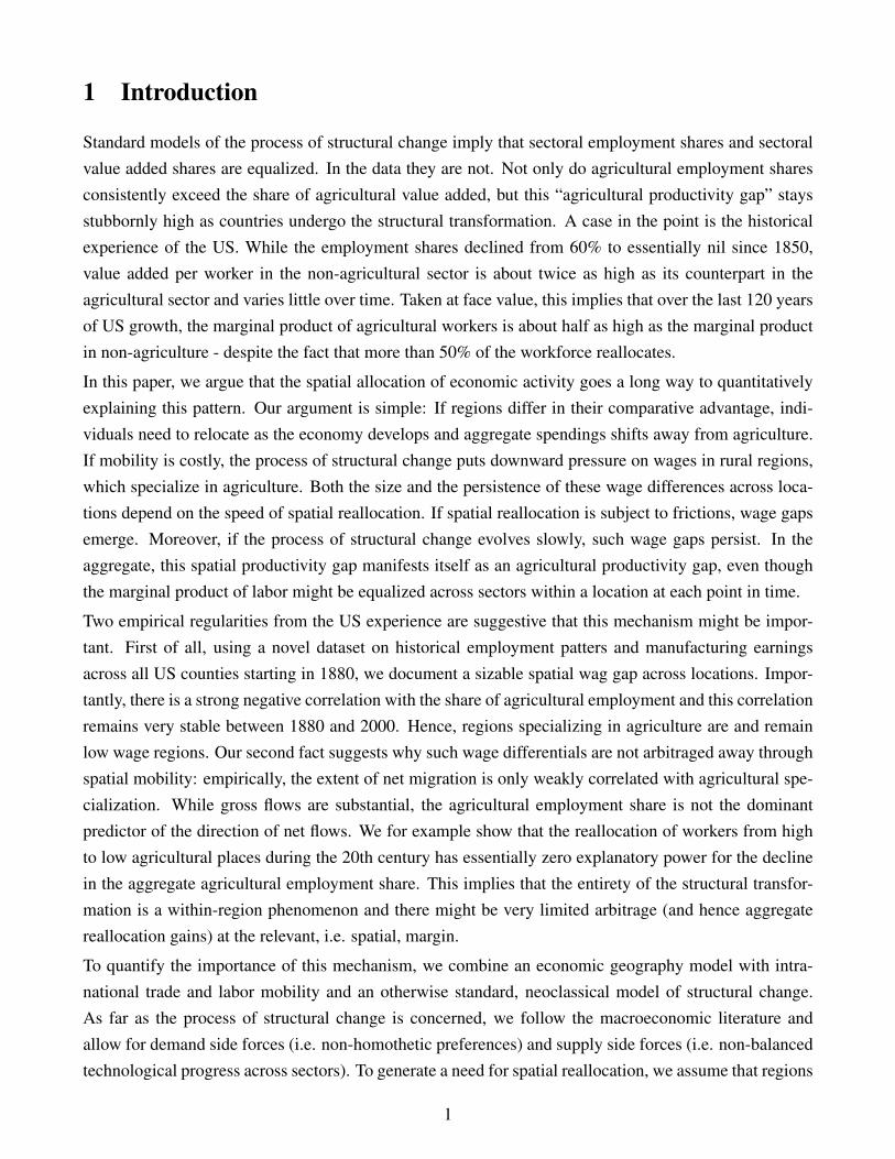
In this Section we provide three important empirical regularities, which suggest why the agriculturalproductivity gap could be a spatial gap. Consider first Figure 1, where we use aggregate data to displaythe time series of the agricultural employment share (blue line) and relative agricultural productivity, i.e.value added per worker in agricultural relative to non-agriculture, for the US economy since 1850. Whileagricultural employment declines sharply, relative agricultural productivity is essentially constant andonly half as large as productivity in the non-agricultural sector. This is inconsistent with most macroeco-nomic models of the structural transformation, where sectoral value added per worker is proportional tothe wage, which is equalized across sectors - see e.g. Herrendorf et al. (2014).1

0

.2

.4

.6

.8

1

1.2

Rel

ativ

e Pr

oduc

tivity

in A

gric

ultu

re0

.2

.4

.6

Agric

ultu

ral E

mpl

oym

ent S

hare

1850 1900 1950 2000Year

Notes: The figure shows the aggregate agricultural employment share (blue line) and value added per worker in agriculturalrelative to value added per worker in non-agriculture (red line).

Figure 1: The Structural Transformation and Agricultural Productivity in the US

In Figure 2 we report three empirical regularities about the spatial aspects of the structural transformation,which highlight why this agricultural productivity gap could be a spatial gap. In the left panel, wedepict the cross-sectional correlation between agricultural employment shares and average earnings since1880.2 We see that this correlation is strongly negative in 1880 and that it remains negative for theentirety of the 20th century. The fact that the correlation between average earnings and agriculturalemployment stays negative despite the fact agricultural employment declines drastically suggests thatspatial mobility is not the main driver for the process of structural change. The second panel in Figure 1

1To see this more formally, suppose that production in sector s takes place according to Ys = AsF (k, l), where F hasconstant returns to scale and all markets are competitive. This implies that the capital intensity is equalized. Hence,

VAs

Ls=

PsAsF (Ls,Ks)

Ls= w× F (k,1)

∂F(Ls,Ks)∂L

= w× F (1,k)∂F(1,k)

∂L

,

i.e. value added per worker is equalized across sectors.2In the paper, we use the definition of a commuting zone as our definition of a region. There are roughly 700 commuting

zones in the US. We describe our data in more detail in Section 5 below.

5

shows in what sense there indeed is an absence of “spatial arbitrage”.In particular, we report the impliedagricultural employment share, which emerged solely from spatial reallocation. More specifically, weconduct a “shift-share”-analysis, by fixing regional agricultural employment shares at their 1880 leveland calculate the aggregate agricultural employment share using the population distribution from thedata.3 This is the red line in the middle panel of Figure 1. For comparison we again superimpose theactual agricultural employment share from Figure 1 in blue. It is clearly seen that - in an accounting sense- spatial reallocation accounts for essentially nothing of the aggregate decline in agricultural employment.To put it differently, the process of the structural transformation is not driven by a reallocation of peoplefrom high to low agricultural places. Conversely, most of structural change seems to take place within

regions. That this is indeed the case is seen in the right panel of Figure 2, where we display the cross-sectional distribution of regional agricultural shares for different years. There is a marked leftwardsshift, whereby all regions see a decline in agricultural employment. Hence, the structural transformationtransforms places and is not merely a process which reallocates production factors across space.

-1

-.6

-.2

.2

.6

1

1880 1910 1940 1970 2000Year

Correlation of Earnings and Ag Employment

Across Component

Ag. Empl. Share

0

.2

.4

.6

.8

1

1880 1910 1940 1970 2000Year

Structural Change across Regions

188019101940

1970

0

2

4

6

0 .2 .4 .6 .8 1Agricultural Employment Share

Structural Change within Regions

Notes: In the left panel we show the correlation between the agricultural employment share and average earnings across UScommuting zones. In the middle panel we show the aggregate agricultural employment share (blue line) and the predictedagricultural share holdings regional agricultural shares at their 1880 level, i.e. ∑r sA,r,1880× lr,t , where sA,r,t and lr,t are theagricultural employment share and the population share of region r at time t. In the right panel we show the cross-sectionaldistribution of agricultural employment shares in different years. For a detailed description of the construction of the regionaldata we refer to Section 5.

Figure 2: Spatial Structural Change: Three Facts

The patterns in Figure 1 are qualitatively consistent with an important role for the spatial allocation ofresources in explaining the persistence of the agricultural productivity gap. Regions who specialize inagriculture are places with low wages on average and spatial arbitrage is too slow a process for suchspatial wage gaps to disappear. Finally, the fact that the vast majority of labor reallocation takes placewithin regions, implies that the sharp decline in aggregate agricultural employment is perfectly consistentwith persistent difference in average productivity if marginal products within locations are equalized. Inthis paper, we argue that the facts displayed in Figure 1 are also quantitatively consistent with the observedaggregate productivity gap displayed in Figure 1. This, of course, requires a structural model, which iswhere we turn now.

3More precisely, we calculate this series as ∑sA,r,1880×Lr,tLt

, where sA,r,1880 is the regional agricultural employment sharein 1880 and Lr.t is number of workers in region r.

6

3 Theory

In this section we present our theory of spatial structural change. The theory rests on three pillars. We startwith an essentially neoclassical model of the structural transformation, where the process of structuralchange is generated from non-homothetic demand and unbalanced technological progress. We introducea spatial dimension, by embedding this structure into an economic geography model of heterogeneouslocations and costly spatial mobility. Finally, we allow for skill-based selection across locations andsectors of production by assuming that individuals differ in their human capital and skilled workers haveboth an absolute advantage and a comparative advantage in the non-agricultural sector.

3.1 Environment

Technology We consider an economy with two goods, an agricultural good and a non-agriculturalgood. For simplicity we also sometimes refer to the latter as the manufacturing good. Each good is a CEScomposite of differentiated regional varieties with a constant elasticity of substitution σ . In particular,

Ys =

(R

∑r=1

Yσ−1

σrs

) σ

σ−1

, (1)

where Yrs is the amount of goods in sector s stemming from region rand σ is the elasticity of substitution.Production functions are fully neoclassical and given by

Yrst = ArstKαrstH

1−αrst ,

where Krst and Hrst denotes capital and labor (in efficiency units) in region r, sector s and time t. Forexpositional simplicity, we suppose that capital shares are identical across sectors. We will allow fordifferences in our empirical application. It is useful to express productivity Arst as

Arst = Zst×Qrst with ∑r

Qσ−1rst = 1. (2)

Here, Zst is an aggregate TFP shifter in sector s which affects all regions proportionally. Additionally,there are idiosyncratic sources of productivity. The vector of [Qrs] describes the distribution of regionalproductivity differences, that is the extent to which some regions are more efficient at producing sectors goods compared to other locations. The common components of Qrs across industries captures differ-ences in absolute advantage, i.e. some location might be more efficient to produce all goods. Similarly,regional differences in Qrs/Qrs′ capture differences in comparative advantage. Given the normalizationembedded in (2), we also refer to the Qrs as measuring the heterogeneity in productivity across space.

7

Capital accumulates in the usual way, i.e. according to

Kt+1 = (1−δ )Kt + It ,

where It denotes the amount of investment at time t and δ is the depreciation rate. We assume that theinvestment good is a Cobb-Douglas composite of the agricultural and non-agricultural good given in (1).Letting φ be the share of the agricultural good in the production of investment goods, the price of theinvestment good is given byPI,t = Pφ

A,tP1−φ

M,t . For the remainder we take the investment good to be thenumeraire.

Selection, Human Capital and Labor Supply We allow individuals to differ in their human capital.Doing so is important to credibly measure the agricultural productivity gap if individual skills are cor-related with sectoral sorting.4 In particular, suppose that individuals can be of two types - high skilledand low skilled. Their skill type h determines the distribution of their sector-specific efficiency unitszi =

(zi

A,ziNA

). For tractability, we assume that for each worker i, zi is drawn from the Frechet distribution

Fhzi

s(z) = e−Ψh

s z−ζ

, (3)

where Ψhs parametrizes the average level of human capital of individuals of skill type h in sector s and ζ

governs the dispersion of skills. The empirically relevant case is one where skilled individuals have anabsolute advantage, i.e. ΨH

s > ΨLs for all s and a comparative advantage in the manufacturing sector, i.e.

ΨHNA/ΨH

A > ΨLNA/ΨL

A. A convenient parametrization of these assumption is that5[ΨL

A ΨLNA

ΨHA ΨH

NA

]=

[1 1q qµ

].

Hence, q parametrizes the absolute advantage of skilled individuals and µ governs the complementaritybetween skills and non-agricultural employment.

We assume that - at the aggregate level - a fraction λ of the population is skilled. How people of differentskills are distributed across space is of course endogenous and will be determined endogenously frompeoples’ migration decisions. While individuals know their skills, i.e. h ∈ {L,H} prior to their mobilitydecision, they only learn the actual realization of their efficiency bundle zi afterwards. This structurehas two convenient properties. First of all, individuals differ in their spatial mobility choice only bytheir skill. Allowing mobility to depend on the realization of their efficiency bundle zi would be lesstractable as we would need to keep track of continuum of ex-ante heterogenous individuals. Secondly,this structure retains the convenient aggregation properties of the Frechet distribution in (3). If workers’

4Not surprisingly, such sorting behavior is going to be relevant for our application - we find strong evidence that unskilledindividuals are overrepresented in the agricultural sector.

5Note that ΨLs = 1 is a normalization given the regional technologies Qrs.

8

spatial choice was conditional on zi, the distribution of skills within a location would no longer be of theFrechet form.

Given these assumptions, we can now characterize the individual earnings and aggregate labor supply inlocation r. Let λrt be the endogenous share of skilled individuals working in region r. Total earnings ofindividual i residing in region r are given by

yir = max

{wr,A× zi

A,wr,NA× ziNA}, (4)

where wr,s denotes the prevailing equilibrium wage per efficiency unit in region r. The Frechet distribu-tion implies that average earnings of individual in skill group h are given by

E[yi,h

r

]= Γζ ×Θ

hr ,

where Γζ = Γ(1−ζ−1) and Γ(.) is the gamma function and

Θhr =

(Ψ

hAwζ

r,A +ΨhNAwζ

r,NA

)1/ζ

. (5)

Note that Θhr is equalized across sectors and can be directly calculated from the regional wages

(wr,A,wr,NA

)but differs across skill-types. This endogenous scalar Θh

r will turn out to be a key endogenous object inour analysis and we will refer to it as expected regional income (or for brevity regional income). Inparticular, given Θh

r , the share of people of skill group h employed in the two industries is given by

shs,r = Ψ

hs ×(

wr,s

Θhr

)ζ

, (6)

so that the sectoral labor supply elasticity is governed by ζ . Using (6) is also easy to show that our modelincorporates the consequences of worker selection stressed by Lagakos and Waugh (2011): the average

amount of efficiency units provided to sector s by individuals of skill group h is given by

Hhr,s

Lr× shs,r

=(

shs,r

)− 1ζ

(Ψ

hs

) 1ζ

,

i.e. is decreasing in the sectoral employment share shs,r as individual sorting implies that the marginal

worker in sector s is worse than the average worker.

Demographics In terms of preferences and demographics, we consider an OLG economy. Individualslive for two periods, work when they are young and save to be able to consume when they are old. TheOLG is structure is convenient because it generates a motive for savings (and hence capital accumulation),while still being sufficiently tractable to allow for spatial mobility.

In our model, individuals have three economic choices to make: (i) they decide how much to save and

9

consume, (ii) they allocate their spending optimally across the two consumption goods and (iii) andthey decide where to work and live. In terms of timing, we assume that individuals are born, decide ontheir preferred location when they are young and then remain in that location for their entire life. Theiroffsprings are born in the location where the old generation resides. For simplicity, we abstract fromendogenous human capital accumulation and assume that skills are perfectly inherited, i.e. parents withskill h have children of skill h.

Letting V (et ,Pt) be the indirect utility function of spending an amount et at prices Pt =(PA,t ,PNA,t

),

life-time utility of individual i after having moved to region r is given by

U ir = max

[et ,et+1,s]{V (et ,Pt)+βV (et+1,Pt+1)} , (7)

subject to

et + st = yirt (8)

et+1 = (1+ rt+1)st . (9)

Here, yirt is individual i’s real income in region r (see (4)), st denotes the amount of savings and rt =Rt−δ

is the real interest rate.

Preferences For our model to induce the process of structural change, we have to move away fromhomothetic preferences. In particular, we require a specification of preferences, where consumers reducetheir relative agricultural spending as they grow richer. To do so, we follow Boppart (2014) and assumethat individual preferences can be represented by the indirect utility function

V (e,P) =1η

(e

pφ

A p1−φ

NA

)η

− ν

γ

(pA

pNA

)γ

+ν

γ− 1

η, (10)

This is a slight generalization of the PIGL demand system employed by Boppart (2014).6 This demandsystem has two convenient properties. First of all, it incorporates both income effects (governed by η) andprice effects (governed by γ) in a flexible way. In particular, Roy’s Identity implies that the expenditure

6For V (e, p) to be well-defined, we have to impose additional parametric conditions. In particular, we require that η < 1,that γ ≥ η . These conditions are satisfied in our empirical application. See Section 8.6 of the Appendix for a detaileddiscussion. Boppart (2014) uses this demand system to study the the evolution of service sector. In terms of (10) he assumesthat PA is the price of goods and PNA is the price of services and considers the case of φ = 0.

10

share on the agricultural good, ϑA (e, p), is given by7

ϑA (e, p) ≡ xA (e, p) pA

e= φ +ν

(pA

pM

)γ

e−η . (11)

For η > 0, the expenditure share on agricultural goods is declining in total expenditure. This capturesthe income effect of non-homothetic demand, whereby higher spending reduces the relative expenditureshare on agricultural goods. The long-run secular decline in agricultural employment shown above is toa large extent driving by the increase in income per capita, which shifts aggregate demand away fromagriculture. Holding real income e constant, the expenditure share is increasing in the relative price ofagriculture if γ > 0. The case of η = 0 corresponds to a homothetic demand system, where expenditureshares only depend on relative prices. The case of η = γ = 0 is the Cobb Douglas case where expenditureshares are constant.

We opted for the the preferences specification in (10) for two reasons. First of all, Alder et al. (2017)have shown that while the more popular Stone-Geary specification is unable to quantitatively account forthe long-run process of structural change between 1880 and 2000, a preference specification in the PIGLclass provides a good fit to the long-run data. Secondly, we show below that these preferences allow fora very tractable aggregation despite the fact that they fall outside the Gorman class. Hence, they can beincorporated into a general equilibrium trade model in a tractable way.8

Spatial Mobility Now consider the decision for individual i with skill h to move from j to r. We followthe literature on discrete choice models and assume the value of doing so can be summarized by

U ihjr = Eh [Ur]−MC jr +Ar +κν

ij,

where Eh [Ur] is the expected utility of living in region r (which is conditional on the skill level h), Ur ischaracterized in (15), MC jr denotes the cost of moving from j to r, Ar is akin to a location amenity, whichsummarizes the attractiveness of region r and which is common to all individuals and νh

j is an idiosyn-cratic error term, which is independent across locations and individuals. Furthermore, κ parametrizes theimportance of the idiosyncratic shock, i.e. the extent to which individuals sort based on their idiosyn-cratic tastes relative to the systematic attractiveness of region r. The higher κ , the less responsive areindividuals to the fundamental value of a location embedded in Eh [Ur].

As in in the standard conditional logit model, we assume that νhj is drawn from a Gumbel distribution.

7As we show in detail in Section 8.2 in the Appendix, Roy’s Identity implies that

ϑA (e, p) = xMA (p,e)× pA

e=−

∂V (p,e(p,u))∂ pA

pA

∂V (p,e(p,u))∂e e

,

where xMA (p,e) denotes the Marshallian demand function. For V (p,e) given in (10), this expression reduces to (11).

8This is in contrast to the non-homothetic CES demand system, which has recently been analyzed in Comin et al. (2015).

11

This implies that the share of people with skill type h moving from j to r is given by

ρhjrt =

exp( 1

κ×(Eh [Ur]+Art−MC jr

))∑

Rl=1 exp

( 1κ×(Eh [Ul]+Alt−MC jl

)) , (12)

so that the total number of workers of skill type h in region r is simply

Lhr,t =

R

∑j=1

(ρ

hjrt×Lh

j,t−1

),

i.e. given by the inflows from all children of skilled individuals in all other regions. Note also that theshare of non-movers of skill type h is simply given by ρh

j j. We will show below that Eh [Ur] has a tractableclosed form expression, which makes (12) easy to solve.

3.2 Competitive Equilibrium

Given the environment above, we can now characterize the equilibrium of the economy. We proceed inthree steps. We first characterize the household problem, i.e. the optimal consumption-saving decisionand spatial choice. We then show that the solution to the household problem together with our distri-butional assumptions on individuals’ skills delivers an aggregate demand system, which can write as afunction of a single endogenous variable, despite the fact that our economy does not admit a represen-tative consumer. Finally, we show that the dynamic competitive equilibrium has a structure akin to theneoclassical growth model: given the sequence of interest rates {rt}t , we can solve the entire spatialequilibrium from simple static equilibrium condition. The equilibrium sequence of interest rates can thenbe calculated from households’ savings decisions.

Individual Behavior

Consider first the households’ consumption-saving decision given in (7). The two-period OLG structuretogether with the specification of preferences in (10) has a tractable solution for both the optimal allo-cation of expenditure and the consumers’ total utility Ur. We summarize this solution in the followingLemma.

Lemma 1. Consider the maximization problem in (7), (8) and (9) where V (e,P) is given in (10). The

solution to this problem is given by

eYt (y) = ψ (rt+1)× y (13)

eOt+1 (y) = (1+ rt+1)× (1−ψ (rt+1))× y (14)

Ur =1η

ψ (rt+1)η−1× yη +Λt,t+1 (15)

12

where

ψ (rt+1) =(

1+β1

1−η (1+ rt+1)η

1−η

)−1(16)

Λt,t+1 = −ν

γ

((pA,t

pM,t

)γ

+β

(pA,t+1

pM,t+1

)γ)+(1+β )

(ν

γ− 1

η

).

Proof. See Section 8.1 in the Appendix.

Lemma 1 characterizes the solution to the household problem. Three properties are noteworthy. First ofall, the policy functions for the optimal amount of spending when young (eY

t (y)) and old (eOt+1 (y)) are

linear in earnings. This will allow for a tractable aggregation of individuals’ demands. Secondly, theseexpenditure policies resemble the familiar OLG structure, where the individual consumes a share

eYt (y)y

= ψ (rt+1) =1

1+β1

1−η (1+ rt+1)η

1−η

of his income when young and consumes the remainder (and the accrued interest) when old. In particular,if η = 0, which is the case if demand is non-homothetic (again see Section 3.2 below), we recover thewell-known OLG formulation with log utility where the consumption share is simply given by 1/(1+β ).Importantly, this consumption share only depends on the interest rate rt+1 but not on the relative pricesPt or Pt+1. This is due to our assumption that nominal income e is deflated by the same price index asthe investment good. This is convenient for tractability and akin to the single-good neoclassical growthmodel, where the consumption good and the investment good uses all factors in equal proportions. Forour purposes, this ensures that an increase in the price of investment good, pI,t , makes savings moreattractive but at the same reduces the marginal utility of spending. Finally, overall utility Ur is additiveseparable between income y and current and future prices Pt and Pt+1 (which determine Λt,t+1). Thisproperty will be essential to characterize agents’ optimal spatial choice in a tractable way.

To solve agents’ spatial choice problem, we have to calculate their expected life-time utility Eh [Ur] - see(12). Given that life-time utility is a power function of individual income yi

r and individual income isFrechet distributed with shape ζ and mean Γζ ×Θh

r , expected life-time utility can be calculated as

Eh [Ur] =

[1η

ψ (rt+1)η−1× yη +Λt,t+1

]=

Γη/ζ

ηψ (rt+1)

η−1×(

Θhr

)η

+Λt,t+1.

Substituting this expression into (12) yields the equilibrium spatial choice probabilities as

ρhjrt =

exp(

1κ×(

Γη/ζ

ηψ (rt+1)

η−1×(Θh

r)η

+Art−MC jr

))∑

Rl=1 exp

(1κ×(

Γη/ζ

ηψ (rt+1)

η−1×(Θh

l

)η −MC jl

)) .This expression has two important properties. First of all, note that it does not feature Λt,t+1, which is

13

constant across locations and hence does not determine spatial labor flows. This additive separability offuture prices embedded in Λt,t,+1 is crucial, because it turns individuals’ optimal location choices into astatic problem.9 Moreover, for a given interest rate rt+1, spatial flows only depend on the endogenousvector of regional income

[Θh

rt]

r, which are determined from (static) labor market clearing conditions.This structure allows us to calculate the transitional dynamics in the model with a realistic geography,i.e. with about 700 regions.

Equilibrium Aggregation and Aggregate Structure Change

The spatial equilibrium of economic activity is of course driven by aggregate demand conditions. Oureconomy does not admit a representative consumer, because the PIGL preference specification in (10)falls outside of the Gorman class. In particular, consider a set of individuals i∈S , with spending ei. Theaggregate demand for agricultural products stemming from this set of consumers is given by

PCAS =

∫i∈S

ϑA (ei,P)eidi =(

φ +ν

(pA

pM

)γ ∫i∈S

e−η

ieidi∫i eidi

)×ES ,

where ES =∫

i∈S eidi denotes aggregate spending. Hence, as long as preferences are non-homothetic,i.e. as long as η > 0, aggregate demand does not only depend on aggregate spending ES , but theentire distribution of spending [ei]i matters. Hence, characterizing the aggregate demand function in oureconomy, which features ample heterogeneity through individuals’ skills, their location choice (whichdetermines the factor prices they face) and the actual realization of the skill vector zi, is in principlenon-trivial.

It turns out that our model delivers very tractable expressions for the economy’s aggregate quantities.This is due to three reasons. The distributional assumption on individual skills implies that individualincome yi is Frechet distributed. In Lemma 1 we showed that individuals’ expenditure policy functionsare linear. Hence, individual spending eis also Frechet distributed. And because individuals’ sectoraldemands depend on spending via a power function, we can solve for the term capturing the inequality inspending explicitly. In particular, suppose that ei is distributed Frechet with parameter A and shape ζ . Itis then easy to very that (see Section 8.3 in the Appendix)

∫i∈S

e−η

ieidi∫i eidi

=E[e1−η

]E [e]

= υ×A−η/ζ ,

where υ = Γ

(1− 1−η

ζ

)/Γ

(1− 1

ζ

)is a constant. Hence, aggregate demand is an explicit function of the

dispersion in spending (ζ ) and the level of income (A). Because equilibrium factor prices only determineindividuals’ income (and hence spending) via the parameter A, we can solve for the aggregate demandside of the economy explicitly. In particular the aggregate expenditure share of the set of consumers S

9Note that our assumption of frictionless trade is important for this result - with unrestricted trade costs, future priceswould be location specific and Λt,t+1 would not be constant across space.

14

is given by

ϑA([ei]i∈S ,P

)≡

PCAS

ES= φ + ν

(pA

pM

)γ

×E−η

S ,

where ES = Γζ A1/ζ is mean spending and ν = νΓ

(1− 1−η

ζ

)/Γ

(1− 1

ζ

)1−η

. Hence, the aggregatedemand system is as if it stems from a representative consumer with mean spending ES and an adjustedpreference parameter ν .

We exploit this “almost” aggregation property intensely in computing the model. Recall that our econ-omy, consists of 2×2×R distinct sets of the consumers - two generations, two skill types and R locations.Letting Eh,Y

r,t and Eh,Or,t denote the mean spending of the young and generation with skills h in region r,

Lemma 1 implies that

Eh,Yr,t = ψ (rt+1)Γζ Θ

hr,t and Eh,O

r,t = [(1+ rt)(1−ψ (rt))]Γζ Θhr,t−1.

Note that the amount of spending of the old generation in year t depends on their income earned in periodt−1, their savings rate (1−ψ (rt)) and the accrued interest. The aggregate amount of consumer spendingon agricultural goods is therefore given by

PCAt = φ ×Et + ν

(pA

pM

)γ

×∑r,h

((Eh,Y

r,t

)1−η

λhr,tLr,t +

(Eh,O

r,t

)1−η

λhr,t−1Lr,t−1

), (17)

where Et = ∑r,h

(Eh,Y

r,t λ hr,tLr,t +Eh,O

r,t λ hr,t−1Lr,t−1

)denotes aggregate consumer spending.

Because a fraction φ of total investment spending is spent on agricultural goods and total value added (orGDP) is given by PYt = It +PCt , the agricultural share in value added is given by

ϑA,t =φ It +PCA

tPYt

= φ + ν

(pA

pM

)γ

×∑r,h

((Eh,Y

r,t

)1−η

λ hr,tLr,t +

(Eh,O

r,t

)1−η

λ hr,t−1Lr,t−1

)PYt

. (18)

Moreover, because workers receive a fraction 1−α of aggregate output, we can express aggregate GDPas

PYt =1

1−α×∑

r,hΓζ Θ

hr,tλ

hr,tLr,t . (19)

Equations (18) and (19) highlight two properties. First of all, for a given allocation of people acrossspace, both aggregate income PYt and the agricultural share ϑA,t only depend on the vector of current andpast average regional incomes

[Θh

r,t ,Θhr,t−1

]r. Secondly, these equations highlight the usual demand side

forces of structural change. In particular, consider an allocation where the distribution of individuals byskill is stationary (i.e. λ h

rt = λ hr and Lr,t = Lr) and where regional incomes Θrt grow at rate g. Because

15

spending Eh,gr,t and GDP are then proportional, (18) implies

ϑA,t = φ +ν

(pA,t

pM,t

)γ

×Ξ×PY−η

t ,

where Ξ is an (endogenous) constant. Hence, rising aggregate income PYt will reduce the agriculturalspending share as long as demand is non-homothetic, i.e. η > 0. At the same time, changes in relativeprices will also affect ϑA,t . In our model, the spatial allocation of resources will of course not be stationaryas the economy undergoes the structural transformation. Similarly, regional incomes Θrt will also notgrow at a constant rate. These features of “unbalanced spatial growth” will also affect the agriculturalspending share directly.

Equilibrium

Given the physical environment above, we can now characterize the dynamic competitive equilibrium inour economy. Our assumptions ensure that the analysis remains very tractable. As highlighted above, thekey properties of our theory are that (i) individual moving decisions are static and (ii) that our economygenerates an aggregate demand system as a function of regional incomes

[Θh

rt]

h. This implies that, for agiven path of interest rates {rr}t , we can calculate the equilibrium by simply solving a set of equilibriumconditions.

Consider first the goods market. The market clearing condition for the agricultural good is given by

∑h

wr,AHhr,A = (1−α)×πrAt×ϑ

VAA,t ×PYt , (20)

i.e. total agricultural labor earnings in region rare equal to a constant share of total agricultural revenuein region r. This in turn is equal to region r’s share, πrAt , in aggregate spending on agricultural goods,ϑVA

A,t ×PYt . Standard arguments imply that regional trade shares π are given by

πrAt =

(PrAt

PAt

)1−σ

=

(QrAtw1−α

rAt

)σ−1

∑Rr=1

(QrAtw1−α

rAt

)σ−1 , (21)

i.e. they do neither depend on the identity of the sourcing region, nor the equilibrium interest rate Rt

or the common component of productivity Zst . Rather, a region r’s agricultural competitiveness onlydepends on its productivity QrAt and the equilibrium price of labor in the agricultural market. Similarly,it is easy to verify that regional agricultural labor income is given by

∑h

wrAtHhrAt = LrtΓ

(1− 1

ζ

)wζ

rAt×∑h

λhr Ψ

hs

(Θ

hr

)1−ζ

.

16

Together with the spatial labor supply equation (12) and the corresponding labor market clearing condi-tions for the non-agricultural sector, these equations directly determine the equilibrium levels of regionalincome

[Θh

rt]

h (or alternatively the equilibrium wages).

Finally, we can also directly calculate the remaining macroeconomic aggregates, in particular the dy-namic accumulation of capital. Because the future capital stock is only given by the savings of the younggeneration, we get that

Kt+1 = (1−ψ (rt+1))×∑r,h

Y hr,tλ

hr,tLr,t = (1−ψ (rt+1))(1−α)PYt . (22)

Hence, future capital is simply a fraction 1−ψ (rt+1) of aggregate labor earnings. This proportionalitybetween the aggregate capital stock and aggregate GDP is a consequence of the linearity of agents’consumption policy rules.

It is worthwhile to point out that our model retains many features of the baseline neoclassical growthmodel. In particular, for given initial conditions [K0,Lr,−1,wr−1] and a path of interest rates {rt}t , theequilibrium evolution of wages and people (by skill type) are solutions to the static equilibrium conditionshighlighted above. Given these allocations, the model predicts the evolution of the capital stock accordingto (22). A dynamic equilibrium requires that the set of interest rates {rt}t is consistent with the impliedevolution of the capital stock. More formally, a competitive equilibrium in our economy is defined in theusual way.

Definition 2. Consider the economy described above. Let the capital stock K0, the initial spatial alloca-

tion of people [Lr,−1] and the vector of past wages [wr,−1] be given. A dynamic competitive equilibrium is

a set of prices [Prst ], wages [wrt ], capital rental rates [Rt ], labor and capital allocations [Lrst ,Krst ], con-

sumption and saving decisions[eY

rt ,eOrt ,srt

], sectoral spending shares

[ϑY

rt ,ϑOrt]

and demands for regional

varieties [crst ] such that

1. consumers’ choices[eY

rt ,eOrt ,srt

]maximize utility, i.e. are given by (13) and (14),

2. the sectoral allocation of spending[ϑY

rt ,ϑOrt]

is optimal, i.e. given by (11),

3. the demand for regional varieties follows (21) and firms’ factor demands maximize firms’ profits

4. markets clear,

5. the capital stock evolved according to (22),

6. the allocation of people across space[LY

r,t]

is consistent with individuals’ migration choices in

(12).

17

4 The Spatial Gap

The above model is a model of spatial structural change. It delivers a concise framework to connectthe allocation of factors across space and sectors along the structural transformation. Besides being ofinterest in itself, this paper argues that novel spatial dimension of structural change can in fact explainwhy agricultural productivity at the aggregate level is likely to be persistently low during the structuraltransformation.

We define the agricultural productivity gap as the share of agricultural value added relative to the shareof agricultural employment. In our spatial model, this productivity gap can be written as

GAPt ≡ϑVA

A,t

LA,t/Lt=

∑Rr=1 sArt× yA

rtyrt× yrt×Lrt

∑Rr=1 yrt×Lrt

∑r sArt× Lrt∑r Lrt

. (23)

Here, sA,r and Lrt denote the regional agricultural employment share and the regional population and yrt

and yArt denote regional average earnings and agricultural earnings, respectively, i.e.

yAr =

λrsHA,rΘ

Hrt +(1−λr)ΘL

r sLA,r

sA,tand yr = λrtΘ

Hrt +(1−λrt)Θ

Lrt ,

where all the variables are defined as above. Hence, the aggregate agricultural productivity gap dependson the joint distribution of regional agricultural employment shares sArt , relative agricultural earningsyA

rt/yrt , average regional earnings yrt and the size of the population Lrt . While all these ingredients areof course endogenous to the process of structural change, we will show that the gap implied by (23) canquantitatively go a long way to explain the aggregate productivity gap observed in the US.

To build some intuition why this is the case, suppose there was only absolute advantage but no compara-tive advantage, i.e. µ = 1. This implies that high and low skilled earnings are proportional (ΘH

rt = q×ΘLrt)

and that sectoral employment shares are equalized across skill groups (i.e. sHA,r = sL

A,r = sA,r). Hence, rel-ative agricultural earnings within regions are equalized

(yA

rt = yrt)

and the aggregate productivity gap in(23) reduces to

GAPt =∑

Rr=1 sA,r× Lryr

∑Rr=1 Lryr

∑r sArt× LrtLt

, (24)

where regional income per capita yr is given by

yr = [λr×q+(1−λr)]︸ ︷︷ ︸Human Capital

× ΘLrt︸︷︷︸

MPL

, (25)

i.e. reflects both the skill composition of the regional workforce and average earnings, i.e. the marginalproductivity of labor in region r.

18

These equations are instructive. In particular, they highlight that agricultural productivity is relativelylow if the cross-sectional correlation between agricultural employment shares sA,r and regional incomeper capita yr is negative. Hence, the low aggregate productivity of the agricultural sector might simplyreflect the fact that agricultural intensive regions attract low-skilled individuals

(corr

(sA,r,λr

)< 0)

orthat they have low marginal productivity in all industries, i.e. a low level of productivity QA,r and QNA,r.If yr was equalized across space, there would be no productivity gap. This would for example be the caseif all regions were symmetric.

We can further decompose the variation in earnings ΘLrt . In particular, individual’s sectoral labor supply

function implies that (see (6)) thatΘ

Lrt = wrA,t︸︷︷︸

Skill prices

× s−1/ζ

rAt︸ ︷︷ ︸Selection

,

i.e. total earnings in region r could be low because agricultural skill prices are low or because the shareof workers in the agricultural sector is large. This last term is the selection effect highlighted by Lagakosand Waugh (2011), whereby sectoral specialization reduces the average product of labor through sortingbased on comparative advantage. Because the marginal worker in the agricultural sector is worse thanthe average worker, the larger the share of people working in agriculture, the lower average warnings,holding agricultural skill prices constant.

Finally, equation (24) also highlight why it is appropriate to refer to the agricultural productivity gapas a spatial gap: in case there is only a single region, i.e. R = 1, (24) implies that GAPt = 1, i.e.productivity is equalized across sectors as in the baseline model of structural change. While this isseemingly inconsistent with Lagakos and Waugh (2011), note that they look at physical productivityacross sector. The agricultural productivity gap, however, is evaluated at sectoral prices. If workerselection takes the Frechet form, the productivity and price effect exactly cancel out.10 If, however,there is spatial variation in the extent to which workers sort into different sectors and wages differ acrossregions, the extent of selection does directly determine the agricultural productivity gap. To what extentthis spatial friction is quantitatively important depends on the calibrated model. This is where we turnnow.

5 Quantitative Exercise

We now take the framework above to the data. To do so, we exploit a novel dataset on regional economicdevelopment of the US between 1880 and 2000. We first describe the dataset and provide three basicempirical regularities, which suggest the importance of spatial frictions for the productivity gap in agri-culture. After describing our calibration strategy we then turn to our two main results. First we measurethe spatial gap through the lens of the model. We then consider our counterfactual exercise, where wegauge the importance of the costs of spatial mobility for the agricultural productivity gap.

10We show this formally in Section 9.2 in the Online Appendix.

19

5.1 Data

Our main data sources are the Census of manufacturing for 1880 and 1910, the Micro Census for 1880-2000 and County and City Data Books for 1940-2000. From these sources we construct a data setof total workers [Lrt ]rt , average manufacturing wages [wrt ], and sectoral employment shares

[sA,rt

]rt

for all US counties at 30 year intervals between 1880 and 2000.11 We define the agricultural sectorto comprise agriculture, fishing and mining industries defined according to the 1950 Census Bureauindustrial classification system (outlined in Ruggles et al. (2015)). All remaining employed workers areclassified as non-agricultural workers. We construct average manufacturing wages from county leveltotal manufacturing payroll data and manufacturing head counts obtained from the same source.1213 InAppendix 9.14 table 7 contains a comprehensive list of data sources.

We are interested in structural change within and across regions of the continental US economy. Thisposes the question of what constitutes a meaningful spatial aggregation for local economies in the UnitedStates, which have the potential to experience structural change within them and together cover all USterritory.14 Commuting zones as constructed by Tolbert and Sizer (1996) constitute a meaningful defini-tion of such local economies. They partition the US economy into 741 local labor markets that in 1990maximized commuting flows within and minimized them across. Contrary to counties all of these com-muting zones exhibited non-zero non-agricultural employment shares in 1880 as can be seed in figure 3.Note that in 1880 around half of the workforce is employed in agriculture in the aggregate.

To map our county data to commuting zones we use ARCGis software to construct a crosswalk be-tween counties and 1990 commuting zones for every decade between 1880 and 2000. Using this were-aggregate county level data to commuting zones, employing area weights to allocate county levelallocations wherever counties are split.15

The result of this procedure is a panel data set for 717 continental commuting zones from 1880 to 2000which features sectoral employment shares, total employment and average manufacturing wages. For the

11There are a twelve states which in 1880 were not part of the Union yet (had not obtained statehood), we list them hereand give the year of the accession to the Union: North Dakota (1889), South Dakota (1889), Montana (1889), Washington(1889), Idaho (1890), Wyoming (1890), Utah (1896), Oklahoma (1907), New Mexico (1912), Arizona (1912), Alaska (1959)and Hawaii (1959). We exclude Alaska, Hawaii and Washington D.C. The 1880 Census does report data for counties in allstates, even those that had not yet officially obtained statehood in 1880, with two exceptions: Oklahoma and Hawaii. Weimpute 1880 data for Oklahoma’s counties using a procedure described in Appendix (9.14).

121880 wages: 1880 Census of Manufacturing; 1910 wages: 1920 Census of Manufacturing; 1940 wages: 1947 Countyand City Data Book; 1970 wages: 1970 County and City Data Book; 2000 wages: 2000 County and City Data Book.

131940 is the only year for which we have wage data from the micro census and on the county level from the Census ofManufacturing. Aggregating and averaging the former to the county level leads a worker weighted correlation coefficient ofabout 0.7.

14The requirement for this is a somewhat diversified industrial structure. In the 1880 data there are counties with agriculturalemployment shares of almost 1, making counties a seemingly unsuitable aggregation.

15The United States moved from 2473 counties in 1880 to 3142 counties in 2000. In this process some new counties werecreated by splitting in half an existing one and other new ones created by joining together parts of others. In order to map 1880county level data to 1990 counties and from there to commuting zones, it hence becomes necessary to work with fractionsof counties. We use area weights and the assumption of a uniform distribution of industrial activity across space for thisaggregation. More details in the Appendix.

20

0.843 − 0.9950.773 − 0.8430.673 − 0.7730.565 − 0.6730.379 − 0.5650.032 − 0.379No data

Agricultural Employment Shares across Commuting Zones 1880

1.39 − 3.551.15 − 1.391.00 − 1.150.81 − 1.000.62 − 0.810.22 − 0.62No data

Manufacturing Wages across Commuting Zones 1880

Figure 3: Left Panel: Agricultural Employment Share across US Commuting Zones in 1880. Right Panel:Ration of Local Manufacturing Wages relative to US Median across US Commuting Zones in 1880.

main calibration of the model we employ the cross-sections 1880, 1910, 1940, 1970 and 2000 only andnormalize the size of the workforce to unity in each period. We scale the level of wages to ensure thatincome per capita grows at a constant rate. More details on the the construction of this panel can be foundin online Appendix 9.14.

Beyond this panel, the 1940 version of the decennial Micro Census is a data source of particular im-portance for the paper: it is the most recent Census for which all US counties are available and it isthe first Census for which earnings and education variables are available.16 We define a skilled workeras one with a completed high school degree.17 This pins down the skilled employment share in 1940,λr1940. The next section demonstrates that the structure of the model together with other data inputs issuch that a single cross-section of skill shares is sufficient to infer local skill shares for the remainingcross-sections in the sample. Finally, we use the 1940 Census to compute the US wide skill premiumand a manufacturing skilled employment premium which are used in the calibration below. To that endwe use total pre-tax annual wage and salary income together with the same sector definitions as in theconstruction of the panel to construct the average annual wage of skilled workers relative non-skilledones. The manufacturing skilled employment premium is simply the ratio of the fraction of skilled peo-ple working in manufacturing over the fraction of unskilled workers working in manufacturing out of allunskilled workers.

In the model agents move once in their life time in order to choose a labor market. We use the USdecennial Census Micro data obtained from IPUMS (see Ruggles et al. (2015)) to construct an interstatemigration flow matrix for the cross-sections 1880, 1910, 1940, 1970 and 2000. In a given Census wechoose workers between 26 and 50 years of age, and compute the number of them living in a different

16We use the Public-use Micro Census data compiled and maintained Ruggles et al. (2015). In the publicly availablesamples counties are censored and only become available after 70 years. As a result we cannot identify all counties in Censuscross-sections beyond 1940, which is the cross-section most recently de-censored (2010).

17We assume a direct mapping between skilled employment and education. Choosing a higher education cutoff would resultin a overall skilled worker share in the US below 0.29, which seems unrealistic. We do robustness with lower cutoffs.

21

state from their state of birth. Where we use them state level wages are constructed by aggregating countylevel manufacturing wages from above panel.

We use the data constructed by Alvarez-Cuadrado and Poschke (2011) on the relative price of manu-facturing commodities to agricultural goods directly infer

[PA,tPM,t

]tfrom the data. To map the model more

directly to the data a combined price index for manufacturing and the service sector would be needed.We do not know of the existence of a reliable such series.

Finally, we use micro-data on expenditure patterns from the 1930s to estimate consumer preferences.The Consumer Expenditure Survey in 1936 (“Study of Consumer Purchases in the United States, 1935-1936”) contains detailed information on individual expenditure and allows us to calculate the expenditureshare of food. We exploit this cross-sectional information on expenditure shares and total expenditure toestimate the extent of non-homotheticities in demand, i.e. the parameter η .

5.2 Calibration

In this section we outline our calibration procedure. In Section 9.3 in the Appendix we describe ourcalibration in much more detail. We calibrate the model such that aggregate income per capita growsat a constant rate and that the capital-output ratio is constant. In Section 8.5 in the Appendix, we showthat this implies that interest rates are constant and have a closed form expression. For our counterfactualanalysis, interest rates will of course not be constant.

Skill Supply To parametrize the skill supply, we need values for the supply elasticity (ζ ), the compar-ative and absolute advantage of skilled workers (q and µ) and the initial distribution of skilled workersacross space λr,1880. We define skilled individuals as workers with at least a completed high-school edu-cation in 1940 and hold the aggregate share of skilled workers fixed. For the theory we need the spatialdistribution of skilled workers in 1880, i.e. λr,1880. In the data this object is unobserved, as the 1880 mi-cro census only has information on literacy, but not on schooling. We calibrate this initial allocation byrequiring the model to endogenously perfectly replicate the cross-sectional distribution of skill suppliesin 1940.

The 1940 cross-section of data is the only one for which we observe average manufacturing wages,sectoral employment and the commuting zone level skill share λr,1940. Section 9.3.1 in the Appendixshows how these data inputs can be translated into regional sectoral wages, wrs1940, and human capitalstocks, Hrs1940, conditional on the parameters ζ ,µ,q. This in turn allows us to construct Θx

r,1940 (ζ ,µ,q)

and sxr,s (ζ ,µ,q) for x = H,L.

We calibrate the parameter ζ , i.e. the dispersion in individual productivity, to match the dispersion ofearnings in the 1940 Census data. In particular, the model implies that the variance of log earnings with

22

region-skill cells is given by π2

6 ×ζ−2. We therefore identify ζ from

ζ =π

61/2 ×var(ui

rsh)−1/2

,

where var(ui

rsh

)is the variance of the estimated residuals from a regression of log earnings on region,

sector and skill-group fixed effects.

We calibrate q and µ to match the aggregate skill premium and the aggregate relative manufacturing em-ployment share of skilled workers in 1940. In the 1940 Micro Census data we calculate the unconditionalskill premium by taking the average yearly earnings of all individuals with at least high school educationand dividing it by the equivalent number for all workers with less than high school education, whichyields a skill premium of 1.62. We compute the relative manufacturing employment share of skilledworkers as the non-agricultural employment share of skilled workers relative to the one of unskilledworkers. Empirically, this number is equal to 1.21, i.e. high-skilled individuals are 20% more likely towork outside of agriculture. Note that these measures already incorporate the unbalanced spatial sortingof skilled and unskilled individuals, i.e. they take into account that skilled workers live in high-wage andmanufacturing intensive localities.

Aggregate and Local Productivities and Amenities We calibrate local productivities and amenities[Qrst ,Art ] as structural residuals, i.e. we force the model to match the spatial data perfectly with [Qrst ,Art ]

absorbing any residual variation. In the previous section we showed how to obtain sectoral wages andhuman capital conditional on regional skill shares and a range of other available data and already cali-brated parameters. In section (9.3.1) of the appendix we show that these objects can be used to calculatetrade shares as follows:

πrst =wr,sHr,s

∑r wr,sHr,s.

As a result we can treat πrst as data to obtain Qrst from the expression for trade shares given in (21) whichwe restate here for convenience

πrst =

(Qrst

w1−αrs

)σ−1

∑RJ=1

(Q jst

w1−α

js

)σ−1 withR

∑r

Qσ−1rst = 1

Together with sectoral wages and the parameters (σ ,α), this equation along with our normalizationidentifies Qrst exactly.18

18To see the role of Qrst as structural residuals more directly note we can rewrite (21) as follows:

logπrst

π1st= (σ −1) log(Qrst/Q1st)+(1−σ)(1−α) log(wrst/w1st)

23

Recall that we only observe skill shares on the county level in 1940. It turns out the structure of themodel provides sufficient restrictions to imply skill shares, λrt , for every other cross-section given λ1940.Skill shares and amenities are calibrated jointly using equation (12) which allows for the construction ofa useful mapping

Ak+1rt = f ({Θh

rt ,Lhrt ,L

hrt−1,A

krt}h=L,H) with ∑

rAr = 0

The algorithm to jointly back out skill shares and amenities is then as follows: (1) Use 1940 skill sharesfrom the data to calculate Θh

rt . (2) Guess skill shares in 1910 and use worker stocks in 1910 to calculateLh

rt−1. Then we iterate on f to get implied amenities Art . Since these amenities are not indexed by skilltype they may imply a Lh

rt−1 that yields skill shares for 1910 different from our initial guess. We iteratebetween updating skill shares and amenities until convergence. (3) We then guess skill shares for 1970and use the f mapping forward to obtain 1970 and 2000 skill shares and amenities: this time guessingskill shares three decades ahead, calculating implied amenities by iterating on f and then updating theskill share guess. This procedure leaves us with a panel of skill shares and amenities for all commutingzones and cross-sections. More details can be found in section 9.3.1 in the Appendix. In figure 14 in theAppendix we plot the densities of the calibrated [Qrst ,Art ] for every cross-section.

Lastly, we calibrate the time series of aggregate sectoral productivities, [ZAt ,ZMt ], to match the evolutionof relative prices and a GDP growth rate of 2%. We plot these two implied series in figure 15 in theAppendix.

Moving Costs We specify moving frictions as a quadratic function of distance as follows:

τi j =

τ if j = i

δ1di j +δ2d2i j if j 6= i

τ > 0 corresponds to a fixed cost of moving: if a worker decides to move away from his commutingzone of birth he forgoes the place utility τ . Additionally movers have to pay a cost, denominated inutils, that varies with the distance travelled. We normalize di j so that the maximum distance in the US is1. Before this normalization the largest distance between two continental commuting zone centroids is2827.4 miles.

In the Census data we observe for every decade and for every individual her state of birth and her currentstate of residence. Using this we can construct a lifetime state-to-state migration flow matrix. For ourbaseline estimates we would like to choose (κ,τ,δ1,δ2) so as to match these state to state flows asclosely as possible for the 1910-1940 period, while still matching local populations, employment sharesand wages exactly.

Regressing trade shares (now observed) on wages yields the log ratio of Qrst as a structural residual. The necessity of anadditional normalization then also becomes clear. We choose ∑

Rr Qσ−1

rst = 1 since this choice helps to simplify certain analyticexpressions.

24

Since our model features commuting zones while our data records state to state flows we will aggregatecommuting zone flows to the state level in the model and calibrate (κ,τ,δ1,δ2) so as to make the modelfit state to state flows as closely as possible.

Consider the flow equation from the model:

Lhr,t = ∑

jρ

hjr,t×Lh

j,t−1

where ρhjr is given in equation 12. Also note:

ρhj j

ρhjr=

exp( 1

κ×(Eh [U j

]+ τ +A j

))exp(

1κ×(

Eh [Ur]−δ1d jr−δ2d2jr +Ar

))So that the number of stayers relative to movers increases monotonically in τ for fixed Al . Note thatconsth

j is independent of moving cost parameters given that we always match local labor supply exactly.The procedure for estimating (κ,τ,δ1,δ2) is then to guess (κ,δ1,δ2), compute commuting zone flowsand aggregate them to the state level. For each guess τ is chosen so as to ensure the model matchesthe aggregate interstate migration rate of 0.3 exactly. We then search over combinations of (κ,δ1,δ2) toidentify the tupel that minimizes the following objective:

Λ = ∑i

∑j 6=i

Li,1940×(

logρDATAi j,1940− logρ

MODELi j,1940 (κ,δ1,δ2)

)2

The objective function Λ is a destination population weighted sum of the percentage difference betweenmodel and data of the inflows from all states except the destination itself. We evaluate this objectivefunction over a wide grid for (κ,δ1,δ2) and find that it is well behaved and in particular exhibits a uniqueminimum.

Note that for any guess of (κ,δ1,δ2) we resolve for skilled employment shares in 1910 and the amenityvector in 1940 so as to match skilled employment in 1940 as well as total populations in 1910 and 1940exactly.

Figure 4 shows the density of state level stayers in model and data as well as the distance-flow relation-ship. The model matches the pattern observed in the data quite well. In particular, the model matches thecross-sectional heterogeneity in the share of stayers within a location.

Preferences I: Estimating the non-homotheticity η We use the microdata from the Consumer Expen-diture Survey in 1936 (“Study of Consumer Purchases in the United States, 1935-1936”) to estimate theextent of non-homotheticities. The demand system implies that expenditure shares at the individual levelare given by ϑA (e, p) = φ +ν

(pApM

)γ

e−η . For φ ≈ 0, this implies that there is a log-linear relationship

25

-1.5

-.5

.5

1.5

2.5

Log

Inte

rsta

te F

low

s

0 .2 .4 .6 .8 1Normalized Distance

0

1

2

3

.2 .4 .6 .8 1Fraction of Stayers 1910-1940 (States)

Notes: In the right panel we plot the distribution of the share of people staying in their home state in the data (blue) and model (red). To construct the leftpanel, we run a gravity equation of the form

ρ jr

1−ρ j j= α j +αr +δ1×d jr +δ2×d2

d j +u jr

where ρ jr denote the share of people moving from j to r, α j and αr denote origin and destination fixed effects and d jr denotes the distance between j and r.We run the regression both in the model (red line) and in the data (blue line) and then plot the predicted values.

Figure 4: State-to-state migration: Model vs Data

between expenditure shares and total expenditure, i.e.

lnϑA (e, p) = f (p)−η× lne. (26)

Note that the intercept f (p) is a function of prices but does not vary in the cross-section of households.

In Figure 5 we depict the cross-sectional distribution of the expenditure share for food (left panel) andthe binned scatter plot between (the log of) expenditures and expenditure shares after taking our a set ofregional fixed effects, which are supposed to proxy for f (p). The slope of the regression line is exactlythe extent of the demand non-homotheticity η . It is clearly seen that there is substantial heterogeneityin the expenditure share on food in the cross-section of households. Moreover, the expenditure shareis systematically declining in the level of expenditure and the cross-sectional relationship is essentiallylog-linear as predicted by the theory. The slope coefficient implied that η = 0.32. In Section 9.3 in theAppendix we also report the regression results, when we do not impose the restriction that φ = 0 andestimate the demand function using non-linear least squares. The parameter η is precisely estimated and- depending on the specification - between 0.3 and 0.34.

Preferences II: Estimating (φ ,ν ,γ) In contrast to η , which is estimated from the cross-sectional rela-tionship, we use the time-series of the aggregate agricultural employment share to identify the remainingparameters (φ ,ν ,γ). As γ determines the price elasticity of demand, we discipline γ with the elasticity ofsubstitution. In particular, the model implies that the elasticity of substitution of individual i is given by

σESi = 1−η− (γ−η (1−φ))(1−φ)

1−ϑA,i+

[γ +φη ]φ

ϑA,i.

26

0.0

2.0

4.0

6

0 .2 .4 .6 .8 1Expenditure share for food

-.4-.2

0.2

.4ln

food

sha

re

-1.5 -1 -.5 0 .5 1ln expenditure

Notes: The figure shows the cross-sectional distribution of the individual expenditures shares on food (left panel) and the binscattered relationship between the (log) expenditure share on food and (log) total expenditure as in (26) (right panel). Therelationship in the right panel is conditional on a set of location and family size fixed effects. The underlying data stems fromthe Study of Consumer Purchases in the United States, 1935-1936.

Figure 5: Expenditure Shares on Food in 1936

Hence, the elasticity of substitution varies across households and across time. Comin et al. (2015) esti-mate this elasticity to be around 0.7 in post-war data for the US. We therefore chose γ so that the modelimplies an average elasticity of substitution of 0.7 in the year 2000.

Given our calibration strategy for the underlying distribution of productivity and amenity fundamentals,internal consistency requires us to match these four agricultural employment shares exactly. As wediscuss in detail in Section 9.13 in the Appendix, the income effects as implied from the cross-sectionalspending-food relationship displayed in Figure 5 are not strong enough to explain the entire decline inagricultural employment in the time-series.19 We therefore allow the parameter φ to be time-specific tofully account for the residual decline in agricultural employment and chose ν to minimize the requiredtime-variation in φt . Intuitively, ν is chosen for the model to explain as much of the aggregate process ofstructural change as possible, given the income and price elasticities η and γ . Note that φ does not enterthe household’s decision problem directly. This strategy, which we explain in detail in Section 9.10 ofthe Appendix, yields parameter estimates, which are reported in Table 1.

Endogenous Amenities In our counterfactuals we allow amenities to be a function of local populationLr. In particular we assume that the overall amenity in location r can be written as:

Ar,t = ρLθr,t + Ar,t (27)

where Ar is the exogenous component of the amenity inherent to location r and ρ,θ ∈ R flexibly param-eterize the endogenous effect of local population on amenities. It is natural to think about a congestive

19This discrepancy between the cross-section and time-series is not particular to our application. For example, the resultsreported in Comin et al. (2015) also imply different estimates for the income elasticity stemming from the cross-section andthe time-series. While reconciling this discrepancy between the cross-section and the time-series is an important open researchquestion, it is not the main focus or our paper.

27

effect of local population on local amenities as in Ahlfeldt et al. (2015) and Allen and Arkolakis (2014)and our estimates will imply this.

Similar to Ahlfeldt et al. (2015), notice that for each set of parameters of the model, there is a uniquevector Ar,t for each t = 1910,1940,1970,2000 such that the observed vectors of wages, local populationsand employment shares in each cross-section are an equilibrium of the model. This result is independentof (ρ,θ). In order to estimate (ρ,θ) we first fit the model to the data and back out the full panel ofamenities Ar,t for t = 1910,1940,1970,2000. We then rewrite 27 in differences:

∆Ar,t = ρ∆Lθr,t +∆Ar,t (28)

In equation 28 {∆Ar,t ,∆Lr,t}r=1,...,R,t=1910(30)2000 are observed independently of (ρ,θ). With an instru-ment ϕr,t for ∆Lθ

r,t that induces variation in local population inflows between t and t − 1 orthogonal to∆Ar,t the two parameters (ρ,θ) could be obtained by minimizing the sample equivalent of the followingmoment condition:

E[ϕr,t∆Ar,t

]= E

[ϕr,t

(∆Ar,t−ρ∆Lθ

r,t

)]= 0

To construct such an instrument we turn to a Model Implied Optimal IV (MOIV) general equilibriumestimator as recently proposed by Adao et al. (2017). We simulate the model for a given guess of (ρ,θ)holding the implied Ar,1880 fixed throughout but letting all other fundamentals vary as calibrated. Thisgenerates a series of population changes ∆Lr(∆Qr,s,t ,∆Ar,t = 0,∆Zs,t | θ ,ρ) which is by constructionorthogonal to changes in Ar,t .

Λ = ∑t=1940,1970,2000

[1N ∑

r∆Lr,t(∆Qr,s,t ,∆Ar,t = 0,∆Zs,t | θ ,ρ)∆Art

]2

Other parameters Finally, we need values of the capital share α , the rate of depreciation δ , the pref-erence parameter σ and the consumers’ discount rate β . For (α,σ ,δ ) we we take central values from theliterature. We take a capital share of 1/3. This implies that our model is consistent with the aggregatelabor share of 2/3, which is relatively constant during our time-period. We assume an annual rate ofdepreciation of 8%. Finally, we chose σ = 4. We also target an investment rate of 15% and a growthrate of 2%, both of which are consistent with the aggregate US experience in the 20th century. Thesemoments directly determine β .

5.3 Calibration Results

In Table 1 we report the calibrated parameters and the main targeted moment, both in the data and themodel. Naturally, the parameters are calibrated jointly.

An important part of our calibration strategy is that we calibrate the cross-sectional distribution of sectoralproductivities

{QA,rt ,QNA,rt

}r and amenities {Art}r as structural residuals. Hence, given the remaining

28

Para

met

erTa

rget

Valu

eM

omen

tsD

ata

Mod

el

Skill

Supp

lyζ

Skill

hete

roge

neity

Res

idua

lEar

ning

sva

rian

cein

1940

1.62

0.62

0.62

ξSh

are

ofsk

illed

indi

vidu

als

Shar

ew

ithm

ore

than

high

scho

olde

gree

in19

400.

30.

30.

3µ

Com

para

tive

adva

ntag

eR

el.n

on-a

g.sh

are

ofsk

illed

wor

kers

in19

403.

411.

211.

21q

Abs

olut

ead

vant

age

Skill

prem

ium

in19

400.

681.

621.

61[λ

r,188

0]In

itial

dist

ribu

tion

ofsk

illed

indi

vidu

als

Skill

dist

ribu

tion

in19

40.

{λr,1

940}

mat

chda

tape

rfec

tly

Reg

iona

lFun

dam

enta

ls[Q

rAt]

rst

Agr

icul

tura

lpro

duct

ivity

Reg

iona

lem

pl.s

hare

san

dea

rnin

gsSe

eA

ppen

dix{e

Man

r,t,s

A,r

t}m

atch

data

perf

ectly

[QrN

At] r

stN

on-a

gric

ultu

ralp

rodu

ctiv

ity[A

rt] r

tA

men

ities

Reg

iona

lpop

ulat

ion

{Lh r,t}

Tim

eSe

ries

Impl

icat

ions

[ZN

At]

Non

-agr

icul

tura

lpro

duct

ivity

Agg

rega

tegr

owth

rate

ofG

DP

pcSe

eA

ppen

dix

2%2%

[ZAt]

Agr

icul

tura

lpro

duct

ivity

Rel

ativ

epr

ice

ofag

.goo

dsSe

eA

ppen

dix{P

A,t/P

NA,t}

mat

chda

tape

rfec

tly

Pre

fere

nce

Para

met

ers

βD

isco

untr

ate

Inve

stm

entr

ate

alon

gth

eB

GP

0.29

0.15

0.15

φA

g.sh

are

inpr

ice

inde

xTi

me

seri

esof

ag..

empl

.sha

reSe

eA

ppen

dix

{sA,t}

mat

chda

tape

rfec

tlyν

PIG

LPr

efer

ence

para

met

erTi

me

seri

esof

ag..

empl

.sha

re0.

017

0.20

0.20

ηN

on-h

omot

hetic

ityA

g.sh

are

-exp

endi

ture

rela

tions

hip

0.35

0.04

0.04

γPr

ice

sens

itivi

tyE

last

icity

ofsu

bstit

ion

in20

000.

350.

70.

7M

ovin

gC

osts

and

Mob

ility

τFi

xed

cost

sof

mov

ing

Inte

rsta

tem

igra

tion

rate

1.63

0.3

0.3

κD

ispe

rsio

nof

idio

sync

ratic

spat

ialt

aste

sO

bser

ved

stat

e-to

-sta

teflo

ws

0.42

Est

imat

edw

ithN

LS

[δ1,

δ2]

Dis

tanc

e(m

iles)

elas

ticity

ofm

ovin

gco

sts

[8.4

4,−

6.39

]E

stim

ated

with

NL

SO

ther

para

met

ers

δD

epre

ciat

ion

rate

(ove

r30

year

s)se

texo

geno

usly

0.91

.α

Cap

itals

hare

inpr

oduc

tion

func

tion

sete

xoge

nous

ly1/

3.

.

Not

es:T

his

tabl

eco

ntai

nsth

eca

libra

ted

para

met

ers.

Tabl

e1:

Cal

ibra

ted

stru

ctur

alpa

ram

eter

s

29

Dependent Variablelog Pop. (lnLr) Agr. empl. share (sA,r) log manufac. earnings

Productivity (lnQNA,r) 0.522∗∗∗ -0.019∗∗∗ 0.138∗∗∗

(0.032) (0.004) (0.007)

Comparative Adv. (lnQA,r/QNA,r) -0.042 0.022∗∗∗ 0.038∗∗∗

(0.036) (0.004) (0.007)

Amenities (Ar) 0.567∗∗∗ 0.007 -0.164∗∗∗

(0.080) (0.011) (0.017)

Year FE Yes Yes YesObservations 2580 2580 2580R2 0.916 0.783 0.995

Notes: Robust standard errors in parentheses with ∗∗∗, ∗∗ and ∗ respectively denoting significance at the 1%, 5% and 10% levels. The dependent variablesare the structural residuals “productivity” (lnQNA,r), “comparative advantage (lnQA,r/QNA,r)” and “Amenities” (Art ), which are inferred from the calibratedmodel. The regressions are run for the years 1910, 1940, 1970 and 2000.

Table 2: Fundamentals and Endogenous Outcomes

parameters reported in Table 1, the model matches the population distribution, the regional agriculturalemployment shares and average manufacturing earnings exactly. In Table 2 we report three descriptiveregressions to illustrate the model’s mapping form unobserved fundamentals to observed endogenousoutcomes. In particular, we run regression of the form

yrt = δt + γ× lnQNA,rt +β × ln(

QA,rt

QNA,rt

)+α×Art +urt ,

where yrt denotes the endogenous outcomes at the regional level, i.e. population size, agricultural em-ployment shares or manufacturing earnings. For ease of interpretation, we project these outcomes onthe level of productivity

(QNA,rt

), the comparative advantage in agriculture and regional amenities. We

find that (i) regional size is mostly driven by the level of productivity and regional amenities, that (ii) aregions’ agricultural employment share is negatively correlated with regional productivity and positivelycorrelated with comparative advantage in agriculture and that (iii) manufacturings earnings are positivelycorrelated with productivity and comparative advantage but negatively correlated with amenities.

6 Results

With the calibrated model at hand, we can now answer the two questions we set out to address. In Section6.1 we ask to what extent the calibrated model can account for the observed agricultural productivity gapat the aggregate level. We also provide a decomposition into the different regional fundamentals. InSection 6.2 we then quantify the importance of spatial mobility costs. In particular, we show that thespatial gap would not have been markedly lower in the absence of moving costs and we also explain why

30

0

.2

.4

.6

.8

1

1.2

The

Ag. P

rodu

ctiv

ity G

ap

1880 1910 1940 1970 2000Year

Model GapAggregate Gap (Data)Naive Gap

Notes: The figure shows the agricultural productivity gap as implied by the calibrated model (red line), the agricultural productivity gap from the aggregatedata (blue line) and the “naive spatial gap”, which we calculate as GAPNaivs

t =(

∑r sA,rt × eMrt Lrt

∑r eMrt Lrt

)/LA,t , where eM

rt denotes the average manufacturingearnings from the data.

Figure 6: The Spatial Agricultural Productivity Gap in the US from 1880 - 1910

this is the case.

6.1 The Spatial Gap in the US from 1880 to 2000

With the quantitative model we can now calculate the implied spatial gap by evaluating (23). The resultis contained in Figure 6 below. In red we display the implied agricultural gap by the model. It is seenthat the model implies that value added per worker is substantially lower in agriculture than in non-agriculture, even though there are - by construction - no sectoral labor frictions. For comparison we alsodepict the productivity gap as measured in the aggregate data (and reported in Figure 1) as the blue line.Hence, Figure 6 shows that our model can comfortably explain between 50% and 70% of productivitydifferences between sectors without resorting to frictions across industries.

Because our model is calibrated to perfectly rationalize the data on employment shares and manufacturingearnings, the question is to what extent Figure 6 is informative about the mechanism of the model. Tosee that the model indeed adds explanatory power for the implied agricultural gap, the black line inFigure 6 shows the implied productivity gap from a “naive” exercise, which abstracts from human capitaldifferences and treats observed manufacturing earning as skill-adjusted wages.In particular, suppose onecalculates the productivity gap

GAPNaivet =

∑r sA,rt× eMrt Lrt

∑r eMrt Lrt

∑r sA,rt× Lrt∑r Lrt

, (29)

where eMrt denotes the observed average manufacturing earnings in region r. Note that (29) can be cal-

culated directly from the data. As can be seen from Figure 6, the implied productivity gap is much

31

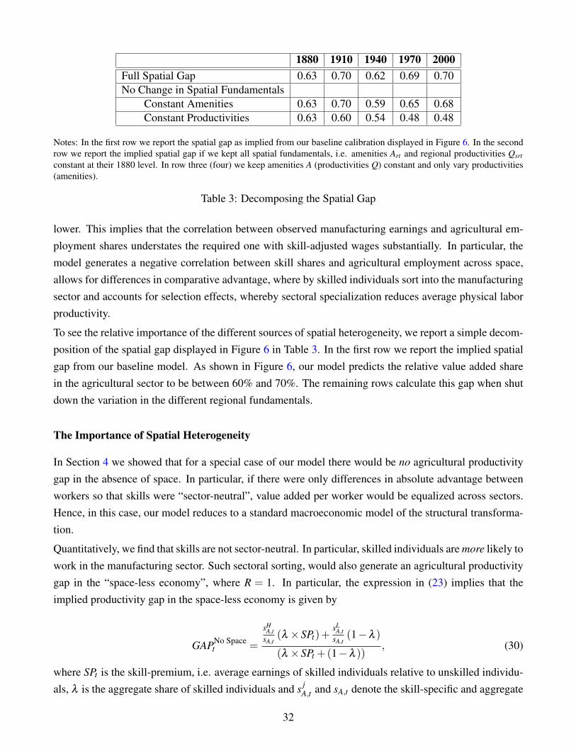
1880 1910 1940 1970 2000Full Spatial Gap 0.63 0.70 0.62 0.69 0.70No Change in Spatial Fundamentals

Constant Amenities 0.63 0.70 0.59 0.65 0.68Constant Productivities 0.63 0.60 0.54 0.48 0.48

Notes: In the first row we report the spatial gap as implied from our baseline calibration displayed in Figure 6. In the secondrow we report the implied spatial gap if we kept all spatial fundamentals, i.e. amenities Art and regional productivities Qsrtconstant at their 1880 level. In row three (four) we keep amenities A (productivities Q) constant and only vary productivities(amenities).

Table 3: Decomposing the Spatial Gap

lower. This implies that the correlation between observed manufacturing earnings and agricultural em-ployment shares understates the required one with skill-adjusted wages substantially. In particular, themodel generates a negative correlation between skill shares and agricultural employment across space,allows for differences in comparative advantage, where by skilled individuals sort into the manufacturingsector and accounts for selection effects, whereby sectoral specialization reduces average physical laborproductivity.

To see the relative importance of the different sources of spatial heterogeneity, we report a simple decom-position of the spatial gap displayed in Figure 6 in Table 3. In the first row we report the implied spatialgap from our baseline model. As shown in Figure 6, our model predicts the relative value added sharein the agricultural sector to be between 60% and 70%. The remaining rows calculate this gap when shutdown the variation in the different regional fundamentals.

The Importance of Spatial Heterogeneity

In Section 4 we showed that for a special case of our model there would be no agricultural productivitygap in the absence of space. In particular, if there were only differences in absolute advantage betweenworkers so that skills were “sector-neutral”, value added per worker would be equalized across sectors.Hence, in this case, our model reduces to a standard macroeconomic model of the structural transforma-tion.

Quantitatively, we find that skills are not sector-neutral. In particular, skilled individuals are more likely towork in the manufacturing sector. Such sectoral sorting, would also generate an agricultural productivitygap in the “space-less economy”, where R = 1. In particular, the expression in (23) implies that theimplied productivity gap in the space-less economy is given by

GAPNo Spacet =

sHA,t

sA,t(λ ×SPt)+

sLA,t

sA,t(1−λ )

(λ ×SPt +(1−λ )), (30)

where SPt is the skill-premium, i.e. average earnings of skilled individuals relative to unskilled individu-als, λ is the aggregate share of skilled individuals and s j

A,t and sA,t denote the skill-specific and aggregate

32

0

.2

.4

.6

.8

1

1.2

The

Ag. P

rodu

ctiv

ity G

ap

1880 1910 1940 1970 2000Year

Spaceless EconomySpatial Economy

Notes: The figure shows the agricultural productivity gap for the spatial model (red line) and the spaceless economy (blueline). As explained in the text, both models are calibrated to the same aggregate time-series data.

Figure 7: The Importance of Space

agricultural employment shares. Hence, if high skilled individuals have higher earnings (SPt > 1) andare less likely to work in agriculture, there will be a gap as relative value added per worker in agricultureis relatively low. Again that there would be no gap if sectoral employment shares were equalized acrossskill-groups.

It is useful to express the skill-specific relative agricultural employment shares as a function of the shareof skilled individuals λ , the aggregate agricultural share sA,r and the manufacturing share of high-skilledindividual relative to low-skilled individuals. As we show in Section 9.12 in the Appendix, this yields

sLA,t

sA,t=

sA,t +λ × (MSHt−1)(λ ×MSHt +(1−λ ))sA,t

andsH

A,t

sA,t=

sA,t− (1−λ )(MSHt−1)(λ ×MSHt +(1−λ ))sA,t

, (31)

where MSHt = sHNA,t/sL

NA,t is the relative non-agricultural employment share of high-skilled individuals.Hence, the productivity gap in the space-less economy is fully determined by

{sA,r,SPt ,MSHt

}t .

To calculate the implied spatial gap in the spaceless economy, we calculate GAPNo Spacet given the model-

implied skill premium and relative manufacturing share from our spatial economy. Hence, the spatialand the spaceless economy are calibrated to the exact same data. In Figure 7 we compare the impliedproductivity gap of the spatial model with the spaceless economy. The red line is again the spatialgap depicted in Figure 6. The blue line shows the productivity gap in the spaceless economy, which iscalibrated to the exact same aggregate time-series moments as the spatial economy. As Figure 7 clearlyshows: the implied productivity gap from the spaceless economy is only half as large as the one impliedby the spatial economy. Hence, the spatial gap displayed in Figure 6 is to a large extent due to space andnot only a function of the sectoral skill-composition.

33

0

.2

.4

.6

.8

1

Inte

rsta

te M

igra

tion

Rat

e

1880 1910 1940 1970 2000Year

0

.2

.4

.6

.8

1

1.2

The

Ag. P

rodu

ctiv

ity G

ap

1880 1910 1940 1970 2000Year

Notes: In the left panel we show the interstate migration rate in the baseline model (blue line) and in an economy withoutcosts of spatial mobility (red line). In the left panel we display the spatial gap in the baseline model (blue line) and in aneconomy without costs of spatial mobility (red line).

Figure 8: The (Non)-Importance of Spatial Mobility Costs

6.2 The Importance of Spatial Moving Costs

The results above highlight that differences in factor prices across space are highly persistent, i.e. thatthere is little spatial arbitrage between agricultural-intensive and manufacturing-intensive locations. Anatural culprit of such wage gaps are the existence of moving costs, MC jr. To analyze to what extentsuch moving costs are the fundamental driver of the low productivity in agriculture, we now consider acounterfactual exercise and calculate the agricultural productivity gap, if spatial mobility was free (i.e.τ = δ = 0).

Doing so naturally increases the amount of spatial mobility substantially. In particular, the share ofindividuals, who do not change their location after birth drops essentially to zero. This is natural: in thepresence of idiosyncratic regional taste shocks and with more than 700 locations to choose from, it isvery unlikely that any given individual considers her original location the preferred one. One implicationof these patterns of spatial mobility is a sharp increase in the interstate migration rate. In the left panel ofFigure 8, we show the time-series of the interstate migration rate in the baseline economy (blue line) andin counterfactual economy without moving costs - if there were no moving costs, the interstate migrationrate was close to 100%.

In the right panel of Figure 8 we display the implied spatial gap. Again we superimpose the results of thebaseline calibration for comparison. These lines are strikingly similar. Hence, the sharp increase in spatialmobility does not raises relative agricultural productivity. This was only the case if spatial net flowstended to be negatively correlated with agricultural employment as such flows will increase agriculturalwages relative to non-agricultural wages holding the fundamentals fixed. In our counterfactual economywith free mobility this does not occur in equilibrium.

34

Why do not lower moving costs reduce the spatial gap?

The underlying explanation for the patterns shown in Figure 8 is simple: in our economy (as apparentlyin the data) there are ample reasons move other than wage differences induced by differences in thesectoral structure. In particular, idiosyncratic tastes and regional amenities are powerful determinantsof individual location choices. If mobility was costless, these consideration would still be powerful anddissociate the equilibrium net flow of people from the extent of agricultural specialization.

To see this more clearly, consider a streamlined version of our model. In particular, suppose (i) thatthere are no amenity differences (Art = 0 for all r, t), (ii) that there is no skill heterogeneity (q = µ = 1),(iii) that regional productivity is constant at its 1880 level (Qs,r,t = Qs,r,1880) and (iv) that moving costsare only parametrized by the fixed costs of moving τ (δ = 0). This structure implies that individuals’mobility incentives are determined from the fixed costs of moving (τ) and the dispersion of idiosyncraticpreference shocks (κ). While the former parametrizes the ease of moving, the latter determines thedirection of flows conditional on moving, i.e. the correlation between wage differences and regionalflows.20

In Figure 9 we show the implied spatial gap for the case of free mobility (i.e. τ = 0) and the estimatedvalue of the fixed moving costs if individuals mostly care about earnings rather than locations per se, i.e.for κ ≈ 0. Figure 9 clearly shows that in such environments, spatial mobility is an arbitraging force. Ifmobility was free, the agricultural gap would indeed decline. In fact, without spatial mobility acting asa balancing force, relative agricultural productivity would decrease along the structural transformation.This pattern is closely related to the pattern in the spaceless economy shown in Figure 7 above. As thestructural transformation in itself is an aggregate force that puts pressure on agricultural regions through adecline in the demand for agricultural products, spatial mobility is an important margin for the aggregateeconomy to adjust.

However, empirically, individuals have locational preferences other than regional factor prices and ourstructural estimation reveals that these considerations are important. Hence, the empirically relevantcase is the one of κ > 0. If, however, such considerations are important, spatial mobility is no longeran arbitraging force. To see this concretely, consider the case of Memphis County. In 1880, MemphisCounty has a workforce of about 800.000 individuals, 75% of which worked in the agricultural sector. Atthe time, this put Memphis County at 67 percentile of the distribution of agricultural employment sharesin the US.

How do migration patterns of the model-residents in Memphis county in 1880 look like? In Figure 10

20To see this formally, note that the share of people from skill group h moving from j to r, ρhjr, satisfies

ρ jr

1−ρ j j=

exp(

1κ

(Γη/ζ

ηψ (rt+1)

η−1 (Θh

r)η))

∑l 6=r exp(

1κ

(Γη/ζ

ηψ (rt+1)

η−1 (Θh

l

)η)) ,

i.e. the probability of moving from j to r conditional only depends on κ .

35

.5

.6

.7

.8

.9

1

1.1

The

Ag. P

rodu

ctiv

ity G

ap

1880 1910 1940 1970 2000Year

Costly Mobility (τ=τ*)Free Mobility (τ=0)

Notes: This figure shows the implied spatial gap in the simplified model for a high and low level of moving costs τ

Figure 9: Arbitrage if Spatial Tastes are Unimportant (κ ≈ 0)

0

.2

.4

.6

.8

1

Shar

e of

Mov

ers

to le

ss A

gric

ultu

ral C

Z

0

.2

.4

.6

.8

1

Shar

e of

Mov

ers

0 .1 .2 .3 .4 .5 .6κ

Memphis Commuting Zone, 1880

Notes: This figure shows the share of people moving out of Memphis county (blue line, left axis) and the share of movers whomove to regions with an agricultural share exceeding the one in Daniels count (green line, right axis).

Figure 10: Mobility Out of Memphis County in 1880

we depict these patterns as a function of the importance of the idiosyncratic shock κ for the estimatedlevel of fixed costs τ∗. The blue line displays the share of young residents of Memphis County who moveto a new location. It is clearly seen that mobility out of Memphis County increases in the dispersion ofidiosyncratic tastes. At the same time, less movers from Memphis County actually move towards regions,with a smaller agricultural sector. As the red line shows, for small levels of κ , everyone who leavesMemphis County heads towards a less agricultural location. As κ increases, more people move and moreof these actually relocate to regions with a higher agricultural employment share. Our structural estimatessuggest that the US in the 20th century resembled much more a high-κworld, where the correlationbetween net population flows and agricultural employment shares is small. In such a world, spatialarbitrage is limited and lower costs of moving are unlikely generate large economic gains of reallocation.

36

7 Conclusion

The process of structural change is characterized by two salient regularities: a marked decline in theagricultural employment share and a persistent agricultural productivity gap, whereby agricultural valueadded per worker is consistently lower than in the non-agricultural sector. These facts are inconsistentwith the vast majority of models of structural change. Moreover, the persistence of the agricultural pro-ductivity gap despite the fact that the structural transformation induces a large reallocation of productionfactors, suggests that sectoral frictions might not be the major culprit.

In this paper, we argue that the agricultural productivity gap could in fact be a spatial gap. If regionsdiffer in their comparative advantage, individuals need to spatially relocate as the economy develops andaggregate spendings shifts away from agriculture. If this process of spatial reallocation is costly, spatialwage gaps emerge. In particular, manufacturing-intensive regions will have to pay higher wages to attractagricultural workers from afar. This spatial correlation between agricultural specialization and equilib-rium directly implies a sectoral productivity gap. Moreover, if agricultural specialization is only weaklycorrelated with net population outflows, this spatial agricultural productivity might be very persistent,even though the marginal product of labor might be equalized across sectors within a location at eachpoint in time.

We show that this mechanism can go a long way to explain the agricultural productivity gap quantita-tively. On the theoretical side, we introduce a novel model of spatial structural change by embedding aneconomic geography model with costly labor mobility into a dynamic, neoclassical model of the struc-tural transformation. We rely on a non-homothetic demand system of the PIGL class as considered inBoppart (2014). Combined with the canonical Frechet-structure of skill heterogeneity, this preferencestructure remains highly tractable, despite falling outside the Gorman class.

As our application, we study the growth experience of the US between 1880 and 2000. Using a noveldataset on earnings, sectoral employment shares and the number of workers across US commuting zones,we find that the model can comfortably explain 50% of the agricultural productivity gap observed in theaggregate data. Because the sectoral reallocation of production factors takes place almost entirely withinlocalities, this implies that the macroeconomic gains from worker reallocation are much more modestthan the agricultural productivity gap as inferred from aggregate data suggests.

37

References

Acemoglu, Daron and Veronica Guerrieri, “Capital deepening and nonbalanced economic growth,”Journal of political Economy, 2008, 116 (3), 467–498.

Adao, Rodrigo, Costas Arkolakis, and Federico Esposito, “Trade, Agglomeration Effects, and LaborMarkets: Theory and Evidence,” Mimeo, Yale University, 2017.

Ahlfeldt, Gabriel M, Stephen J Redding, Daniel M Sturm, and Nikolaus Wolf, “The economics ofdensity: Evidence from the Berlin Wall,” Econometrica, 2015, 83 (6), 2127–2189.

Alder, Simon, Timo Boppart, and Andreas Muller, “A Theory of Structural Change that Can Fit theData,” 2017.

Allen, Treb and Costas Arkolakis, “Trade and the Topography of the Spatial Economy,” The Quarterly

Journal of Economics, 2014, 129 (3), 1085–1140.

Alvarez-Cuadrado, Francisco and Markus Poschke, “Structural change out of agriculture: Labor pushversus labor pull,” American Economic Journal: Macroeconomics, 2011, 3 (3), 127–158.

and Ngo Van Long, “Capital-labor substitution, structural change and growth,” CIRANO-Scientific

Publications 2011s-68, 2011.

Baumol, William J, “Macroeconomics of unbalanced growth: the anatomy of urban crisis,” The Ameri-

can Economic Review, 1967, pp. 415–426.

Boppart, Timo, “Structural Change and the Kaldor Facts in a Growth Model With Relative Price Effectsand Non-Gorman Preferences,” Econometrica, 2014, 82 (6), 2167–2196.

Bryan, Gharad and Melanie Morten, “Economic development and the spatial allocation of labor: Evi-dence from Indonesia,” Manuscript, London School of Economics and Stanford University, 2015.

, Shyamal Chowdhury, and Ahmed Mushfiq Mobarak, “Underinvestment in a profitable technol-ogy: The case of seasonal migration in Bangladesh,” Econometrica, 2014, 82 (5), 1671–1748.

Caselli, Francesco and Wilbur John Coleman II, “The US structural transformation and regional con-vergence: A reinterpretation,” Journal of Political Economy, 2001, 109 (3), 584–616.

Chenery, Hollis B, “Patterns of industrial growth,” The American Economic Review, 1960, 50 (4), 624–654.

Comin, Diego, Danial Lashkari, and Martı Mestieri, “Structural Change with Long-Run Income andPrice Effects,” 2015. Working Paper.

38

Desmet, Klaus and Esteban Rossi-Hansberg, “Spatial Development,” American Economic Review,2014, 104 (4), 1211–43.

, David Krisztian Nagy, and Esteban Rossi-Hansberg, “The Geography of Delevopment: EvaluatingMigration Restrictions and Coastal Flooding,” 2015. Working Paper.

Fajgelbaum, Pablo and Stephen J Redding, “External integration, structural transformation and eco-nomic development: Evidence from argentina 1870-1914,” 2014. Working Paper.

Fajgelbaum, Pablo D, Eduardo Morales, Juan Carlos Suarez Serrato, and Owen M Zidar, “Statetaxes and spatial misallocation,” Technical Report, National Bureau of Economic Research 2015.

Gollin, Douglas, David Lagakos, and Michael E Waugh, “The Agricultural Productivity Gap,” Tech-nical Report, Quarterly Journal of Economics 2013.

, Stephen Parente, and Richard Rogerson, “The Role of Agriculture in Development,” American

Economic Review, 2002, 92 (2), 160–164.

Herrendorf, Berthold, Richard Rogerson, and Akos Valentinyi, “Two perspectives on preferencesand structural transformation,” The American Economic Review, 2013, 103 (7), 2752–2789.

, , and Ákos Valentinyi, “Growth and Structural Transformation,” Handbook of Economic Growth,2014, 2, 855–941.

Hsieh, Chang-Tai and Enrico Moretti, “Why do cities matter? Local growth and aggregate growth,”Technical Report, National Bureau of Economic Research 2015.

Kongsamut, Piyabha, Sergio Rebelo, and Danyang Xie, “Beyond balanced growth,” The Review of

Economic Studies, 2001, 68 (4), 869–882.

Kuznets, Simon, “Quantitative aspects of the economic growth of nations: II. industrial distribution ofnational product and labor force,” Economic Development and Cultural Change, 1957, pp. 1–111.

Lagakos, David and Michael E Waugh, “Selection, Agriculture and Cross-Country Productivity Dif-ferences,” Agriculture and Cross-Country Productivity Differences (November 1, 2011), 2011.

, Mushfiq Mobarak, and Michael E Waugh, “The Macroeconomics of Rural-Urban Migration,”2015.

Michaels, Guy, Ferdinand Rauch, and Stephen J Redding, “Urbanization and structural transforma-tion,” The Quarterly Journal of Economics, 2012, 127 (2), 535–586.

Nagy, Dávid Krisztián, “City location and economic development,” 2016. Working Paper.

39

Ngai, L Rachel and Christopher A Pissarides, “Structural change in a multisector model of growth,”The American Economic Review, 2007, 97 (1), 429–443.

Redding, Stephen and Esteban Rossi-Hansberg, “Quantitative Spatial Economics,” 2016. WorkingPaper.

Redding, Stephen J and Daniel M Sturm, “The costs of remoteness: Evidence from German divisionand reunification,” LSE STICERD Research Paper No. PEPP11, 2005.

Ruggles, Steven, Matthew Sobek, Trent Alexander, Catherine A Fitch, Ronald Goeken, Patri-cia Kelly Hall, Miriam King, and Chad Ronnander, “Integrated Public Use Microdata Series: Ver-sion 6.0 [dataset]. Minneapolis: University of Minnesota, 2015,” 2015.

Tolbert, Charles M and Molly Sizer, “US commuting zones and labor market areas: A 1990 update,”1996.

Tombe, Trevor, Xiaodong Zhu et al., “Trade, migration and productivity: A quantitative analysis ofchina,” Manuscript, University of Toronto, 2015.

Young, Alwyn, “Inequality, the urban-rural gap, and migration,” The Quarterly Journal of Economics,2013, 128 (4), 1727–1785.

40

8 Appendix

8.1 Proof of Lemma 1

Suppose that the indirect utility function falls in the PIGL class, i.e. V (e,P) = 1η

(e

B(p)

)η

+C (P)− 1η

.The maximization problem is

U ir = max

[et ,et+1,s]{V (et ,Pt)+βV (et+1,Pt+1)} ,

subject to

et + st pI,t = yirt

et+1 = (1+ rt+1)st pI,t+1.

Substituting for et+1 yields

U ir = max

et

{V (et ,Pt)+βV

((1+ rt+1)

(yi

rt− et) pI,t+1

pI,t,Pt+1

)}.

The optimal allocation of spending is determined from the Euler equation

∂V (et ,Pt)

∂e= β (1+ rt+1)

pI,t+1

pI,t

∂V (et+1,Pt+1)

∂e.

From above (33) we get that this equation is

eη−1t B(pt)

−η = β (1+ rt+1)pI,t+1

pI,teη−1

t+1 B(pt+1)−η

= β

((1+ rt+1)

pI,t+1

pI,t

)η ((yi

rt− et))η−1

B(pt+1)−η

This yields

yirt− et

et=

((1

1+ rt+1

B(pt+1)/B(pt)

pI,t+1/pI,t

)η 1β

) 1η−1

,

so that

et =1

1+(

φη

t,t+11β

) 1η−1× yi

rt

et+1 =(1+ rt+1) pI,t+1

pI,t

(φ

η

t,t+11β

) 1η−1

1+(

φη

t,t+11β

) 1η−1× yi

rt

41

whereφt,t+1 ≡

11+ rt+1

B(pt+1)/B(pt)

pI,t+1/pI,t.

Hence, (7) implies that

U jr = Vjr (et ,Pt)+βVjr (et+1,Pt+1)

= A jr1ε

(et

B(pt)

)ε

+C (Pt)−1ε+β

(A jr

1ε

(et+1

B(pt+1)

)ε

+C (Pt+1)−1ε

)

= A jr1ε

wεrt

B(pt)−ε

(1+(

1β

φεt,t+1

) 1ε−1)1−ε

+C (Pt)+βC (Pt+1)−1+β

ε.

This can be written asU jr = A jrwε

rtΦt,t+1 +Λt,t+1,

where

Φt,t+1 =1ε

B(pt)−ε

(1+(

1β

φεt,t+1

) 1ε−1)1−ε

Λt,t+1 = C (Pt)+βC (Pt+1)−1+β

ε.

For our specification we have that ε = η and B(pt) = pφ

A,t p1−φ

NA,t = 1. Hence,

φt,t+1 ≡B(pt+1)

B(pt)(1+ rt+1)=

11+ rt+1

= φt+1

and

Φt,t+1 =1η

1+(

1β

(1

1+ rt+1

)η) 1η−1

1−η

=1η

(1+β

11−η (1+ rt+1)

η

1−η

)1−η

.

Note also thatet =

1

1+(

φη

t,t+11β

) 1η−1×wt =

1

1+β1

1−η (1+ rt+1)η

1−η

×wt .

This proves the results for Lemma 1.

8.2 Consumption expenditure shares

We can derive the expenditure shares from the indirect utility function Vjr (e, p) in (10) from Roy’sidentity. The indirect utility function is defined by

V (p,e(p,u)) = u.

42

Hence,∂V (p,e(p,u))

∂ p j+

∂V (p,e(p,u))∂e

∂e(p,u)∂ p j

= 0.

The expenditure function is given by

e(p,u) = minx ∑ p jx s.t. u(x)≥ u.

Hence,∂e(p,u)

∂ p j= x j (p,u) ,

where x j (p,u) is the Hicksian demand function. We also have that the Hicksian and the Marshalliandemands are linked via

xH (p,u) = xM (p,e(p,u)) .

Hence,∂V (p,e(p,u))

∂ p j+

∂V (p,e(p,u))∂e

xMj (p,e(p,u)) = 0

Rearranging terms yields

xMj (p,e(p,u)) =−

∂V (p,e(p,u))∂ p j

∂V (p,e(p,u))∂e

.

The expenditure share on good j is therefore given by

ϑ j (e, p) = xMj (p,e)×

p j

e=−

∂V (p,e(p,u))∂ p j

p j

∂V (p,e(p,u))∂e e

. (32)

We consider an indirect utility function from the PIGL class

V (e,P) =1ε

(e

B(p)

)ε

+C (P)− 1ε.

We get that

∂Vr j

∂e= eε−1B(p)−ε (33)

∂Vr j

∂ p j= −eεB(p)−ε−1 ∂B(p)

∂ p j+

∂C (p)∂ p j

.

43

(32) therefore implies that

ϑ j (e, p) =eεB(p)−ε−1 ∂B(p)

∂ p jp j− ∂C(p)

∂ p jp j

eε−1B(p)−ε e

=∂B(p) p j

∂ p jB(p)−

∂C (p) p j

∂ p jC (p)C (p)

(e

B(p)

)−ε

= ηBj −η

Cj ×(

eB(p)

)−ε

C (p) ,

where ηBj and ηC

j are the price elasticities of the B and C function respectively.

The specification we consider is

V (e,P) =1η

(e

pφ

A p1−φ

M

)η

− ν

γ

(pA

pM

)γ

− 1η+

ν

γ.

Hence, we have that

∂V∂e

=

(e

pφ

A p1−φ

M

)η

1e

∂V∂ pA

= −φ

(e

pφ

A p1−φ

M

)η

1pA−ν

(pA

pM

)γ 1pA

.

Hence,

xA (e, p) = φepA

+ν

(pA

pM

)γ 1pA

(pφ

A p1−φ

M

)η

e1−η . (34)

The expenditure share is

ϑA (e, p) =xA (e, p) pA

e= φ +ν

(pA

pM

)γ(

e

pφ

A p1−φ

M

)−η

.

8.3 Earning, Expected Earnings and Aggregate Demand

Consider individual i in region r. Given her optimal occupational choice, the earnings of individual i aregiven by

yi = maxs

{ws,rzi

s}.

We assumed that individual productivities are Frechet Distributed, i.e.

Fhzi

s(z) = e−Ψh

s×z−ζ

, (35)

44

where Ψhs parametrizes the average level of productivity of individuals of skill h in region r in sector s

and ζ the dispersion of skills. Hence, the distribution of sectoral earning yisr ≡ ws,r× zi

s is also Frechetand given by

Fyisr(y) = P

(z≤ y

ws,r

)= e−Ψh

s wζs,r×y−ζ

.

Using standard arguments about the max stability of the Frechet, the distribution of total earnings yi isalso Frechet and given by

Fhyi

r(y) = e−(Θh

r)ζ×y−ζ

= e−(

yΘh

r

)−ζ

(36)

where

Θhr =

(∑s

Ψhs wζ

s,r

)1/ζ

=(

ΨhAwζ

A,r +ΨhNAwζ

NA,r

)1/ζ

.

Hence, average earnings of individual i with skill type h in region r are given by

E[yi

r,h

]= Γ

(1− 1

ζ

)×Θ

hr .

From (36) we can derive the distribution of y1−η . As η < 1, we have that

Fy1−η (q) = P(y1−η ≤ q

)= P

(y≤ q1/(1−η)

)= e

−Θζ×(

q1

1−η

)−ζ

= e−(

qΘ1−η

)− ζ

1−η

.

Hence, y1−η is still Frechet. Therefore

∫iy1−η

i di = Lhr ×E

[y1−η

i

]= Lh

r ×Γ

(1− 1−η

ζ

)×(

Θhr

)1−η

= Lhr ×Γ

(1+

η−1ζ

)×(

Θhr

)1−η

.

8.4 Agricultural Demand

In the main text we derived

ϑVAA,t =

φ It +PCAt

PYt= φ + ν

(pA

pM

)γ

×∑r,h

((Eh,Y

r,t

)1−η

λ hr,tLr,t +

(Eh,O

r,t

)1−η

λ hr,t−1Lr,t−1

)1

1−α×∑r,hY h

rtλhr,tLr,t

whereEh,Y

t = ψt+1×Γ

(1− 1

ζ

)Θ

hr,t = ψt+1×Y h

rt .

45

it is also that case that

Eh,Ot = (1+ rt)(1−ψt)×Y h

rt−1 = (1+ rt)(1−ψt)1ψt×Eh,Y

t−1.

Hence, note that

∑r,h

((Eh,Y

r,t

)1−η

λ hr,tLr,t+

(Eh,O

r,t

)1−η

λ hr,t−1Lr,t−1

)1

1−α×∑r,h Y h

rtλhr,tLr,t

= 1(1−α)−1

(ψ

1−η

t+1 ∑r,h(Y h

rt)−η Y h

rtλhr,tLr,t

∑r,h Y hrtλ

hr,tLr,t

+[(1+ rt)(1−ψt)]1−η

∑r,h(Y h

rt−1)−η Y h

rt−1λ hr,t−1Lr,t−1

∑r,h Y hrtλ

hr,tLr,t

)= 1

(1−α)−1

(ψ

1−η

t+1 ∑r,h(Y h

rt)−η Y h

rtλhr,tLr,t

∑r,h Y hrtλ

hr,tLr,t

+[(1+ rt)(1−ψt)]1−η (1+gt)

−1∑r,h

(Y h

rt−1)−η Y h

rt−1λ hr,t−1Lr,t−1

∑r,h Y hrt−1λ h

r,t−1Lr,t−1

)= 1

(1−α)−1

(ψ

1−η

t+1 ∑r,h(Y h

rt)−η

ωhrt +[(1+ rt)(1−ψt)]

1−η (1+gt)−1

∑r,h(Y h

rt−1)−η

ωhrt−1

).

This is the expression in the main text.

8.5 Balanced Growth Path Relationships

Consider a dynamic allocation where GDP grows at a constant rate and the capital output ratio is constant.Static optimality requires that

Rt =αPYt

Kt= α

11−α ∑

Rr=1 wr,tLr,t

Kt. (37)

Hence, a constant capital output ratio directly implies that the return to capital Rt has to be constant.Hence, the real interest on saving is also constant and given by r = R− δ . This also implies that theconsumption rate in (16) is constant and given by

ψ =(

1+β1

1−η (1+ r)η

1−η

)−1. (38)

To solve for the interest rate, note that (22) and (37) imply that

Kt+1

Kt=

(1−ψ)(1−α)PYt

αPYt/R= (1−ψ)

(1−α)

α(r+δ ) .

A constant capital output ratio implies that

Kt+1

Kt=

PYt

PYt= 1+g,

46

where g is the growth rate of the economy. Hence,

1+g = (1−ψ)(1−α)

α(r+δ ) =

(β

11−η (1+ r)

η

1−η

1+β1

1−η (1+ r)η

1−η

)(1−α)

α(r+δ ) . (39)

This equation determines r as a function of parameters.

Along the BGP the consumption and investment rate is equal to

PCt = ψ (1−α)PYt +αPYt +(1−δ )α

RPYt

PIt = (1−ψ)(1−α)PYt− (1−δ )α

RPYt .

Using (39) yieldsPItPYt

= (g+δ )α

Rand

PCt

PYt= 1− (g+δ )

α

R.

From (39) we also get that

ψ = 1− α

1−α

1+gR

. (40)

8.6 Regularity Conditions for the preferences to be well-defined

In our model, expenditure share on the two goods are given by

ϑA (e, p) = φ +ν

(pA

pM

)γ

e−η

ϑNA (e, p) = 1−φ −ν

(pA

pM

)γ

e−η .

For these expenditure shares to be positive, we need that

ϑA (e, p)≥ 0⇒ eη ≥−ν

φ

(pA

pM

)γ

, (41)

and

ϑNA (e, p)≥ 0⇒ eη ≥ ν

1−φ

(pA

pM

)γ

.

Note first that (41) is trivially satisfied as long as ν > 0. Also note that satisfying both of these restrictionsautomatically implies that ϑs (e, p)≤ 1. In addition, as we show in Section 10.1 in the Online Appendix,for the Slutsky matrix to be negative semi definite, we need that

ν (1−η)

(pA

pM

)γ

− (1−φ)φ

ν

(pA

pM

)−γ

e2η ≤ (1−2φ − γ)eη .

47

Hence, for our preferences to be well-defined, we require that

eη ≥ ν

1−φ

(pA

pM

)γ

(42)

(1−2φ − γ)eη +(1−φ)φ

ν

(pA

pM

)−γ

e2η ≥ ν (1−η)

(pA

pM

)γ

. (43)

Lemma 3. A sufficient condition for (42) to be satisfied is that (43) holds and that

γ > (1−φ)η . (44)

Proof. Equation (43) can be written as

eη − ν

1−φ

(pA

pM

)γ

+(1−φ)φ

ν

(pA

pM

)−γ

e2η ≥ ν (1−η)

(pA

pM

)γ

+(2φ + γ)eη − ν

1−φ

(pA

pM

)γ

eη

ν

1−φ

(pApM

)γ −1

ν

1−φ

(pA

pM

)γ

+φeη

ν

1−φ

(pApM

)γ eη ≥ [(1−φ)(1−η)−1]ν

1−φ

(pA

pM

)γ

+(2φ + γ)eη

eη

ν

1−φ

(pApM

)γ −1

+φeη

ν

1−φ

(pApM

)γ

eη

ν

1−φ

(pApM

)γ ≥ [(1−φ)(1−η)−1]+ (2φ + γ)eη

ν

1−φ

(pApM

)γ .

Letting x = eη

ν

1−φ

(pApM

)γ , this yields

(x−1)+(φx− (2φ + γ))x≥−(1− (1−φ)(1−η)) .

Now let h(x) = (x−1)+(φx− (2φ + γ))x. Hence, h is strictly concave with a minimum at

h′ (x∗) = 1+φx∗− (2φ + γ)+φx∗ = 0.

Hence,x∗ = 1− 1− γ

2φ< 1.

Also note thath(0) =−1 <−(1− (1−φ)(1−η)) .

Hence, for (43) to be satisfied, it has to be the case that x > x∗ = 1− 1−γ

2φ. Hence, condition (43) implies

(42) if

andh(1) = φ −2φ − γ <−(1− (1−φ)(1−η)) .

Rearranging terms yields (1−φ)η < γ , which is (44).

48

Hence, the preferences are well defined as long (43) is satisfied and (44) holds. Because the RHS of (43)is increasing in e in the relevant range, i.e. as long as (43) is satisfied, this implies that the preferencesare well defined as long as e is high enough.

Now note that eit = ψt+1× yit , where yit denotes total earnings of individual i. From (36) we know that

P(eit ≤ κ) = P(

yit ≤κ

ψt+1

)= e−(Θh

r ψt+1)ζ

κ−ζ

,

where

(Θ

hr ψt+1

)ζ

=(

ΨhAwζ

A,r +ΨhNAwζ

NA,r

)×ψ

ζ

t+1 >(

ΨhAwζ

A,r +ΨhNAwζ

NA,r

)×(

1η

(1+β

11−η

)1−η)ζ

.

Hence, as long as aggregate productivity is high enough, we can make P(eit ≤ κ) arbitrarily small.

8.7 Agricultural Specialization and Population growth

In Figure 2 we showed that the decline in the agricultural employment share in not driven by populationmobility away from agricultural locations. In this section we provide further evidence for this (non-)relationship between past agricultural specialization and subsequent population growth. In particular,we consider a regression of the form

g1880−2000L,r = α +β × s1880

A,r +ur,

where g1880−2000L,r denotes regional population growth between 1880 and 2000 and s1880

A,r denotes the agri-cultural employment share in 1880. The results are contained in Table 4. Columns 1 to 3 show that thereis no significant relationship between agricultural specialization in 1880 and population growth between1880 and 2000. Columns 2 and 3 weigh each regression by their initial population in 1880. In column4 we include a whole set of twenty fixed effects of the initial agricultural share quantiles. While thesefixed effects are jointly statistically significant, their explanatory power is still very small. Figure 11shows this relationship graphically. While population growth tends to be slightly smaller in regions witha high agricultural employment share in 1880, the relationship is not particularly strong and certainly notmonotone.

8.8 Urbanization within and across commuting zones

In Figure 2 we showed that the secular decrease in agricultural employment is a within commuting zonephenomenon. The same pattern holds true for the process of urbanization. The left panel in Figure 12shows the increase in urbanization since 1880. The share of people living in urban areas (i.e. cities withmore than 2500 inhabitants) increases from just shy of 20% in 1850 to more than 50% of the population

49

Dep. variable: Population growth 1880 - 2000Agricultural share 1880 -26.241 -3.702∗

(40.829) (1.917)

log Agricultural share 1880 -0.548(0.658)

Ag quantile FE No No No Yes

Weights No Yes Yes YesObservations 717 717 717 717R2 0.000 0.002 0.000 0.014

Notes: Robust standard errors in parentheses with ∗∗∗, ∗∗ and ∗ respectively denoting significance at the 1%, 5% and 10% levels. Column 4 contains a wholeset of 20 fixed effects for the different quantiles of agricultural employment shares.

Table 4: Agricultural Specialization in 1880 and Population growth 1880-2000

05

1015

20Po

pula

tion

grow

th 1

880

- 200

0

1 2 3 4 5 6 7 8 9 10 11 12 13 14 15 16 17 18 19 20

Notes: The figure shows the average rate of population growth between 1880 and 2000 for 20 quantiles of the agricultural employment share in 1880.

Figure 11: Agricultural Specialization in 1880 and Population growth 1880-2000

50

.1.2

.3.4

.5.6

1840 1860 1880 1900 1920 1940Year

Metropolitan areas Urban areas

.2.3

.4.5

.6

1880 1900 1920 1940Year

Actual urban share Counterfactual urban share

Notes: In the left panel we show the aggregate share of people living in urban areas and metropolitan areas between 1850 and1940. In the right panel, we again show the share of people living in urban areas and counterfactual urban share calculatedaccording to uCF

t = ∑r ur,1880× Lrt∑r Lrt

, where ur,1880 is the urban share in 1880.

Figure 12: Urbanization within and across commuting zones

in 1940. A different measure, the share of people living in metropolitan areas, shows a similar pattern. Inthe right panel we again decompose this time-series evolution into a within and across commuting zonecomponent. In particular, we calculate the counterfactual urbanization as

uCFt = ∑

rur,1880×

Lrt

∑r Lrt,

where ur,1880 is the urbanization rate in commuting zone r in 1880. If the increase in urbanizationstemmed from individuals migrating into high-urbanization commuting zone, this counterfactual urban-ization rate would be close to the actual time series. Figure 12 shows that this is not the case - as forthe agricultural employment share, the cross-commuting zone population flows explain a minor share ofactual increase observed in the data.

To see this within-commuting zone patter of urbanization more directly, consider Figure 13. In the leftpanel we depict the “extensive” margin of urbanization, i.e. the share of counties, which have no urbancenters. Expectedly, this number is declining. Similarly, the right panel shows the distribution of theshare of the urban population across commuting zones conditional on this share being positive. As forthe patterns of agricultural employment depicted in Figure 2 these densities shift to the right, indicatingthat urbanization takes place in all regions in the US.

51

0.2

.4.6

.81

Shar

e of

cou

ntie

s w

ith n

o ur

ban

settl

emen

ts

1850 1860 1870 1880 1900 1910 1920 1930 1940

01

23

4

0 .2 .4 .6 .8 1Share of urban population

1880 1900 1920 1940

Notes: In the left panel we depict the share of counties without any urban areas. In the right panel we show the cross-sectionaldistribution of the share of the urban population across counties.

Figure 13: Urbanization within commuting zones

9 Online Appendix

9.1 Additional derivations on the model with selection

In this section we derive some other properties of the selection model, which are convenient. Recall from(3) that the distribution of individual skills is given by

Fhzi

s(z) = e−Ψh

s×z−ζ

, (45)

where Ψhs parametrizes the average level of productivity of individuals of skill h in region r in sector s

and ζ the dispersion of skills. The following result will turn out to be useful

Lemma 4. Let [xi]ni=1 be distributed iid according to

Fxi (x) = e−Ai×x−ζ

.

Then

E[

xi|xi = maxi

[xi]

]= Γ

(1− 1

ζ

)×

(n

∑i=1

Ai

)1/ζ

. (46)

Note that this object does not depends on i.

Proof. Suppose that i = 1 and let us derive the conditional distribution of x1, conditional that x1 is thehighest

[x j]

j. The joint distribution of[x j]

j is given by

F (x1,x2, ...,x3) =n

∏j=1

F (xi) (47)

52

because of independence. Hence, we get that

P(

x1 ≤ m|x1 = maxj

[x j])

=1

P(x1 = max j

[x j]) ×∫ m

0

n

∏j=2

P(x j < x

)dFx1 (x)

=1

P(x1 = max j

[x j]) ×∫ m

0

n

∏j=2

e−A j×x−ζ

×A1ζ x−ζ−1e−A1×x−ζ

dx

=A1

P(x1 = max j

[x j]) ×∫ m

0ζ x−ζ−1

n

∏j=1

e−A j×x−ζ

dx

=A1

P(x1 = max j

[x j]) ×∫ m

0ζ x−ζ−1e−(∑ j A j)×x−ζ

dx.

Now let us derive P(x1 = max j

[x j])

. We get that

P(

x1 = maxj

[x j])

= P(x j ≤ x1 for all j ≥ 2

)=∫

x1

∂F∂x1

(x1,x1,x1, ..)dx1.

Using (47), we get that

∂F (x1,x2, ...,x3)

∂x1=

∂F (x1)

∂x1×

(n

∏j=2

F (xi)

)= e−A1×x−ζ

A1ζ x−ζ−11 ×

(n

∏j=2

e−Ai×x−ζ

j

)

= A1ζ x−ζ−11 ×

(n

∏j=1

e−Ai×x−ζ

i

)= A1ζ x−ζ−1

1 × e−∑ni Ai×x−ζ

i .

Hence,∫x1

∂F∂x1

(x1,x1,x1, ..)dx1 =∫

x1

A1ζ x−ζ−11 × e−(∑

ni Ai)×x−ζ

1 dx1

=A1

∑ni Ai

∫x1

ζ

(∑ni Ai)

1/ζ

(x1

(∑ni Ai)

1/ζ

)−ζ−1

× e−

x1

(∑ni Ai)

1/ζ

−ζ

dx1

=A1

∑ni Ai

.

Substituting this above yields

P(

x1 ≤ m|x1 = maxj

[x j])

=

(n

∑i

Ai

)×∫ m

0ζ x−ζ−1e−(∑ j A j)×x−ζ

dx

=∫ m

0

ζ

κ

( xκ

)−ζ−1e−(

xκ )−ζ

dx,

53

where κ =(∑ j A j

)1/ζ . This is a Frechet distribution with shape ζ and scale κ , i.e.

Fx1|x1=max j[x j] (m) = e−

x

(∑ j A j)1/ζ

−ζ

= e−(∑ j A j)×x−ζ

.

This implies (46)

Lemma 4 is useful because it allows us to calculate sectoral earnings and the sectoral supply of efficiencyunits. Consider first sectoral earnings. Let yi,h

sr = wrs× zi,hs be the earnings of individual i of skill h in

region r working in sector s. The distribution of earnings is

P(

yi,hsr < y

)= P

(zi,h

s <y

wrs

)= e−Ψh

s×(y

wrs )−ζ

= e−Ψhs wζ

rs×y−ζ

.

Hence, Lemma 4 implies that

E[yi,h

sr |yi,hsr = max

s

{yi,h

sr

}]= Γ

(1− 1

ζ

)×(

∑s

Ψhs wζ

rs

)1/ζ

.

Similarly, the average labor supply in sector s is given by

E[zi,h

s |yi,hsr = max

s

{yi,h

sr

}]= E

[zi,h

s |wrs× zi,hs = max

s

{wrs× zi,h

s

}]= E

[zi,h

s |zi,hs = max

k

{wrk

wrs× zi,h

k

}]

= Γ

(1− 1

ζ

)×

(Ψ

hs + ∑

k 6=sΨ

hk

(wrk

wrs

)ζ)1/ζ

= Γ

(1− 1

ζ

)× 1

wrs×(

∑s

Ψhs wζ

rs

)1/ζ

.

Also, the share of people working in sector s is given by

shs,r = P

(yi,h

sr = maxk

{yi,h

kr

})=

Ψhs wζ

rs

∑s Ψhs wζ

rs

= Ψhs ×

wrs(∑s Ψh

s wζrs

)1/ζ

ζ

.

It is useful to define the endogenous scalar of average earning of skill group h in region ras

Θhr =

(∑s

Ψhs wζ

rs

)1/ζ

.

54

Then we can write the sectoral employment share of skill group h, shsr, as

shsr = Ψ

hs ×(

wrs

Θhr

)ζ

,

the aggregate amount of sectoral earnings of skill group h, wrsHhrs, as

wrsHhrs = Lrλ

hr ×P

(yi,h

sr = maxk

{yi,h

kr

})×E

[yi,h

sr |yi,hsr = max

s

{yi,h

sr

}]= Lrλ

hr Γ

(1− 1

ζ

)×(

shsrΘ

hr

).

Note that we can writesh

srΘhr = Ψ

hs ×wζ

rs

(Θ

hr

)1−ζ

.

Hence,

wrsHhrs = LrΓ

(1− 1

ζ

)wζ

rs×(

λhr Ψ

hs

(Θ

hr

)1−ζ).

Note that the aggregate level of aggregate human capital of individuals of skill h working in sector s inregion r is given by

Hhrh = LrΓ

(1− 1

ζ

)wζ−1

rs ×(

λhr Ψ

hs

(Θ

hr

)1−ζ)

= LrΓ

(1− 1

ζ

)×

(λ

hr Ψ

hs

(wrs

Θhr

)ζ−1)

= LrΓ

(1− 1

ζ

)×

λhr Ψ

hs

(sh

sr

Ψhs

) ζ−1ζ

= LrΓ

(1− 1

ζ

)×(

λhr

(Ψ

hs

) 1ζ sh

sr

ζ−1ζ

).

This also implies that total earnings in sector s in region r are given by

Yrs = ∑h

wrsHhrs = LrΓ

(1− 1

ζ

)wζ

rs×∑h

λhr Ψ

hs

(Θ

hr

)1−ζ

.

55