Spatial Quantification of Groundwater Abstraction in the ... Quantiﬁcation of Groundwater...

Spatial Quantification of GroundwaterAbstraction in the Irrigated Indus Basinby M.J.M. Cheema1,2, W.W. Immerzeel3,4, and W.G.M. Bastiaanssen5,6

AbstractGroundwater abstraction and depletion were assessed at a 1-km resolution in the irrigated areas of the

Indus Basin using remotely sensed evapotranspiration (ET) and precipitation; a process-based hydrological modeland spatial information on canal water supplies. A calibrated Soil and Water Assessment Tool (SWAT) modelwas used to derive total annual irrigation applied in the irrigated areas of the basin during the year 2007. TheSWAT model was parameterized by station corrected precipitation data (R) from the Tropical Rainfall MonitoringMission, land use, soil type, and outlet locations. The model was calibrated using a new approach basedon spatially distributed ET fields derived from different satellite sensors. The calibration results weresatisfactory and strong improvements were obtained in the Nash-Sutcliffe criterion (0.52 to 0.93), bias (−17.3%to −0.4%), and the Pearson correlation coefficient (0.78 to 0.93). Satellite information on R and ET was thencombined with model results of surface runoff, drainage, and percolation to derive groundwater abstraction anddepletion at a nominal resolution of 1 km. It was estimated that in 2007, 68 km3 (262 mm) of groundwaterwas abstracted in the Indus Basin while 31 km3 (121 mm) was depleted. The mean error was 41 mm/year and62 mm/year at 50% and 70% probability of exceedance, respectively. Pakistani and Indian Punjab and Haryanawere the most vulnerable areas to groundwater depletion and strong measures are required to maintain aquifersustainability.

IntroductionQuantification of groundwater abstraction, especially

in arid regions where recharge is genuinely small, isof prime importance for sustainable basin scale water

1Department of Irrigation and Drainage, University ofAgriculture, Fasialabad, Pakistan.

2Corresponding author: Water Management Department, DelftUniversity of Technology, Stevinweg 1, 2628 CN Delft, TheNetherlands; 31-15-2785074; [email protected]

3Future Water, Costerweg 1G, 6702 AA Wageningen, TheNetherlands.

4Department of Physical Geography, University of Utrecht,Utrecht, The Netherlands.

5Water Management Department, Delft University ofTechnology, Stevinweg 1, 2628 CN Delft, The Netherlands.

6eLEAF Competence Center, Generaal Foulkesweg 28, 6703 BSWageningen, The Netherlands.

Received April 2012, accepted January 2013.© 2013, National Ground Water Association.doi: 10.1111/gwat.12027

resources. Long-term groundwater abstractions should notincrease than the recharge but rapid population growthand increased irrigation development for food security hasresulted in exhaustive groundwater abstractions in manyalluvial plains (Foster and Chilton 2003; Shah et al. 2007).Siebert et al. (2010) developed a global inventory ongroundwater which estimated that 43% of the total con-sumptive irrigation water use met through groundwater.Groundwater abstractions are temporally episodic and spa-tially variable and depend upon the crop irrigation needs,surface water availability, and water quality. The spatialvariability in groundwater availability and water require-ment by crops complicate the quantification of abstrac-tions. The Indus Basin is a typical example showing highvariability in land use, climate, canal water availability,soil types, and irrigation practices without any regulationin place to measure the groundwater abstraction.

In the Indus Basin, groundwater is utilized solely orin conjunction with surface water to augment insufficient

NGWA.org Vol. 52, No. 1–Groundwater–January-February 2014 (pages 25–36) 25

and unreliable surface water supplies. Groundwaterabstraction ranged between 40% and 60% of irrigationneeds depending upon land uses (Scott and Shah 2004;Sarwar and Eggers 2006; Arshad et al. 2008). The contin-uous abstractions, in high quantities, can adversely affectthe overall water balance when the average value consis-tently exceeds the recharge over a long period. Therefore,accurate information on spatial groundwater abstractionand depletion is immediately required to support develop-ment of management plans.

The estimation of groundwater abstraction isnormally carried out using the tube well utilizationfactor technique or water table fluctuation method(Maupin 1999; Healy and Cook 2002; Qureshi et al.2003). These methods become less suitable when appliedat basin scale due to the poor spatial density of the pointmeasurements.

Alternatively, data on groundwater abstraction can bederived from hydrological models. The success of thesemodels depends primarily on availability of comprehen-sive input data and how well the models are calibrated(Zhang et al. 2008). Long-term time series datasets withhigh spatial details are difficult to obtain in spatially het-erogeneous basins with a limited gauging network (Siva-palan et al. 2003). Extreme spatiotemporal variability inprecipitation and evapotranspiration (ET) in combinationwith low density surface and groundwater point mea-surements makes models prone to errors, as these pointmeasurements cannot represent the spatial variability.Measurements at few stations and their spatial extrapo-lation for the entire basin may yield unreliable estimatesof water use. The uncertainties associated with the mea-sured input data may also lead to biases in the modelestimations (Srinivasan et al. 2010).

In this study we develop, for the first time, a detailedSoil Water Assessment Tool (SWAT) model applicationthat encompasses the entire transboundary Indus Basinthat operates at a relatively high level of spatial detailand includes all components of the hydrological cycle.The SWAT model allows comprehensive modeling ofanthropogenic interventions in the hydrological cycleincluding irrigation, reservoirs, groundwater abstractions,and a wide variety of agricultural practices. The modelwas parameterized using remote sensing-derived datasetsof elevation, land use and precipitation, and calibratedagainst remotely sensed ET at hydrological response unit(HRU) level.

This paper employs new methods to obtaingroundwater information for each pixel, using satellitemeasurements, GIS system, and hydrological model. Themain objective of the paper is to demonstrate how asmart combination of modeling and remote sensing canbe used to provide more clarity on one of the largestunknowns in the hydrological cycle within the complexityof the Indus Basin. Our method identifies groundwaterhotspot areas at high spatial resolution and consequentlygroundwater-pumping activities are no longer a hiddenpiece of information.

Materials and Methods

Study AreaThe Indus Basin lies between latitude 24◦38′ to

37◦03′N and longitude 66◦18′ to 82◦28′E located in fourcountries (Figure 1). The lifeline of the Indus Basin isthe Indus River that traverses China, Afghanistan, Indiaand Pakistan, moving from upstream to the downstreamend of the basin. The elevations range from 0 to8600 m above mean sea level (a.m.s.l). The basin exhibitscomplex hydrological processes due to variability intopography, rainfall, land use, and water use. The averageannual rainfall varies from less than 200 mm in the desertarea to more than 1500 mm in the north and north-east ofthe basin. The 30-year (1961 to 1990) average referencecrop evapotranspiration (ETo) varies between 650 mm inthe northern parts and 2000 mm in the southern desertareas of the basin.

Water is diverted from the Indus River and itsmajor tributaries (Jhelum, Chenab, Ravi, Beas, and Sutlej)through a network of canals to irrigate the agriculturallands. The main reason for this diversion is rainfallinadequacy to fulfill crop water requirements. However,the availability of canal water is unreliable and that hasmotivated farmers to augment shortages in surface waterby groundwater resources (Shah et al. 2000).

Two agricultural seasons kharif (May to October) andrabi (November to April) are in practice. Wheat is themajor crop grown in rabi . Rice and cotton are the majorcrops of kharif season.

Soil and Water Assessment ToolThe SWAT model is a process-based distributed

hydrological model which provides spatial coverage ofthe hydrological cycle components. A comprehensivedescription of the model can be found in literature (Arnoldet al. 1998; Srinivasan et al. 1998; Neitsch et al. 2005);however, for the convenience of our readers, the SWATmodel is summarized in the following paragraphs.

SWAT provides continuous simulation of ET, per-colation, return flow, storage change, surface runoff,channel routing, transmission losses, crop growth, andsediment transport (Kannan et al. 2011). SWAT wasselected because it represents a simple groundwater reser-voir that acts as an interface between soil moisture inthe unsaturated zone, groundwater storage in the saturatedzone, and surface water systems. The spatial water balanceof the unsaturated zone reads as:

�Sus = SWt − SWo =t∑

i=1

(RSWAT + IRRSWAT + Cr

−ETSWAT − wseep − Qsurf − Qlat)

(1)

where �S us is the change in storage of the unsaturatedzone (mm), SWt is the final soil water content (mm H2O),SWo is the initial soil water content on day i (mm H2O),t is the time (d). RSWAT is the amount of precipitation

26 M.J.M. Cheema et al. Groundwater 52, no. 1: 25–36 NGWA.org

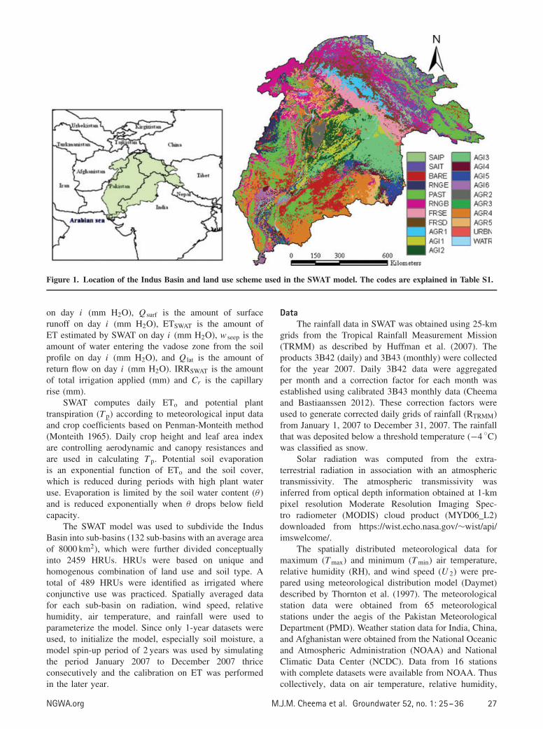
Figure 1. Location of the Indus Basin and land use scheme used in the SWAT model. The codes are explained in Table S1.

on day i (mm H2O), Q surf is the amount of surfacerunoff on day i (mm H2O), ETSWAT is the amount ofET estimated by SWAT on day i (mm H2O), w seep is theamount of water entering the vadose zone from the soilprofile on day i (mm H2O), and Q lat is the amount ofreturn flow on day i (mm H2O). IRRSWAT is the amountof total irrigation applied (mm) and Cr is the capillaryrise (mm).

SWAT computes daily ETo and potential planttranspiration (T p) according to meteorological input dataand crop coefficients based on Penman-Monteith method(Monteith 1965). Daily crop height and leaf area indexare controlling aerodynamic and canopy resistances andare used in calculating T p. Potential soil evaporationis an exponential function of ETo and the soil cover,which is reduced during periods with high plant wateruse. Evaporation is limited by the soil water content (θ )and is reduced exponentially when θ drops below fieldcapacity.

The SWAT model was used to subdivide the IndusBasin into sub-basins (132 sub-basins with an average areaof 8000 km2), which were further divided conceptuallyinto 2459 HRUs. HRUs were based on unique andhomogenous combination of land use and soil type. Atotal of 489 HRUs were identified as irrigated whereconjunctive use was practiced. Spatially averaged datafor each sub-basin on radiation, wind speed, relativehumidity, air temperature, and rainfall were used toparameterize the model. Since only 1-year datasets wereused, to initialize the model, especially soil moisture, amodel spin-up period of 2 years was used by simulatingthe period January 2007 to December 2007 thriceconsecutively and the calibration on ET was performedin the later year.

DataThe rainfall data in SWAT was obtained using 25-km

grids from the Tropical Rainfall Measurement Mission(TRMM) as described by Huffman et al. (2007). Theproducts 3B42 (daily) and 3B43 (monthly) were collectedfor the year 2007. Daily 3B42 data were aggregatedper month and a correction factor for each month wasestablished using calibrated 3B43 monthly data (Cheemaand Bastiaanssen 2012). These correction factors wereused to generate corrected daily grids of rainfall (RTRMM)from January 1, 2007 to December 31, 2007. The rainfallthat was deposited below a threshold temperature (−4 ◦C)was classified as snow.

Solar radiation was computed from the extra-terrestrial radiation in association with an atmospherictransmissivity. The atmospheric transmissivity wasinferred from optical depth information obtained at 1-kmpixel resolution Moderate Resolution Imaging Spec-tro radiometer (MODIS) cloud product (MYD06_L2)downloaded from https://wist.echo.nasa.gov/∼wist/api/imswelcome/.

The spatially distributed meteorological data formaximum (T max) and minimum (T min) air temperature,relative humidity (RH), and wind speed (U 2) were pre-pared using meteorological distribution model (Daymet)described by Thornton et al. (1997). The meteorologicalstation data were obtained from 65 meteorologicalstations under the aegis of the Pakistan MeteorologicalDepartment (PMD). Weather station data for India, China,and Afghanistan were obtained from the National Oceanicand Atmospheric Administration (NOAA) and NationalClimatic Data Center (NCDC). Data from 16 stationswith complete datasets were available from NOAA. Thuscollectively, data on air temperature, relative humidity,

NGWA.org M.J.M. Cheema et al. Groundwater 52, no. 1: 25–36 27

and wind speed from 81 stations were available. Thegridded daily datasets were aggregated per sub-basin,which provided 132 hypothetical meteorological stations(one per sub-basin) with uniform distribution.

A detailed land use and land cover (LULC) mapdeveloped by Cheema and Bastiaanssen (2010) was usedto infer information on different land uses in the IndusBasin. Twenty-seven LULC classes were classified. Thoseclasses were clustered into 21 land use classes based onSWAT land use library. The details of seven irrigated landuse classes including growing season and irrigation depthsare provided in the Table S1.

The actual dates of sowing and harvesting as wellas irrigation depths vary spatially and temporally. Forexample, wheat crop is sown between 1 and 30 Novemberand irrigation depths may vary from 45 to 105 mm, whilenumber of irrigations may vary from 3 to 5. Theseirrigation practices, provided by Pakistan AgriculturalResearch Council (PARC 1982) and Ahmad (2009), wereadopted for initiation of the SWAT model.

The FAO digital soil map of the world (FAO1995) was used to derive soil properties with theaid of pedo-transfer functions (Droogers 2006). Forty-eight different soil units were found in the basin andthe alluvial plains were predominantly characterized byvertisols and the steeper slopes by fluvisols. A GTOPO30-DEM was used in watershed delineation and definingstreams. The surface water supplies at canal heads forvarious canal command areas (CCA) were obtained fromPunjab Irrigation department (PID), Water and PowerDevelopment Authority (WAPDA), and Indus WaterCommission (IWC), Lahore, Pakistan.

ETLookThe ETLook algorithm uses a two-layer Penman-

Monteith equation (Monteith 1965) by dividing each pixelof the image into bare soil and canopy to infer evaporation(E ) and transpiration (T ), respectively (Bastiaanssen et al.2012). The Penman-Monteith equation for E and T canbe written as:

E =�

(Rn,soil − G

) + ρcp

(�e

ra,soil

)

� + γ(

1 + rsoilra,soil

) (2)

T =�

(Rn,canopy

) + ρcp

(�e

ra,canopy

)

� + γ(

1 + rcanopyra,canopy

) (3)

where E and T are in W/m2. G is soil heat flux. �

(mbar/K) is the slope of the saturation vapor pressurecurve which is a function of air temperature (T air,

◦C)and saturation vapor pressure (es, mbar); �e (mbar) isvapor pressure deficit, which is the difference betweenthe saturation vapor content and the actual vapor content;ρ (kg/m3) is the air density and cp is specific heat ofdry air = 1004 J/kg/K; γ (mbar/K) is the psychometricconstant; Rn ,soil and Rn ,canopy are the net radiations

at soil and canopy, respectively; r soil and rcanopy areresistances of soil and canopy, while ra ,soil and ra ,canopy

are aerodynamic resistances for soil and canopy. Allresistances are in s/m. Total ET is the sum of T and E andthe units can be converted to mm/d. In this study, the ETdata is available with an eight day interval for the period ofone calendar year from January 1 to December 31, 2007.

Model Calibration ProcedureThe calibration of the SWAT model was performed

by comparing SWAT modeled ET (ETSWAT) with ETestimated by ETLook at 1-km pixel (ETETLook) forall HRUs. In complex distributed hydrological modelhaving numerous parameters with a high spatial andtemporal heterogeneity, using conventional stream flowcalibration with limited number of discharge stationsmay lead to the equifinality problems, for example, thereare more than one parameter combination leading tosimilar results (Beven and Freer 2001; Beven 2006).Moreover, calibration becomes ineffective in basins, suchas the Indus, where stream flow is under human control(Immerzeel and Droogers 2008).

A stepwise heuristic iterative approach was thereforeadopted to perform calibration by adjusting the key soiland groundwater parameters. A number of importantmodel parameters, which have a large influence on ET,were used in the model calibration. The sensitive param-eters that control E and T fluxes were identified fromthe previous literature (Immerzeel and Droogers 2008;Immerzeel et al. 2008; Githui et al. 2012; Kannan et al.2011). The soil water holding capacity (�), capillary rise(Cr), depth of the evaporation front (�), and the relativewater uptake by plant roots as a function of soil moisture(wup,z ) were calibrated. Their allowable ranges werebound to 0.06 to 0.60 mm/mm for �, 0.02 to 0.9 for Cr,0.01 to 1.0 for � and 0.01 to 1.0 for wup,z (Neitsch et al.2005; Immerzeel and Droogers 2008; Immerzeel et al.2008). �, �, Cr and wup,z coefficients were optimizedfor each HRU. Most parameters were optimized per HRUof each land use class to capture the spatial heterogeneitybecause land use information is available at relativelydetailed level compared with the soil type information.Default values of these parameters were adopted for thebase run and implemented adjustments were constrainedby the ranges of parameters suggested by Neitsch et al.(2005).

Three common statistical indicators, as described byHoffmann et al. (2004), were used to quantify the achievedlevel of calibration and to evaluate the SWAT model’soverall performance. The Nash-Sutcliffe model efficiency(NSE) (Nash and Sutcliffe 1970), Pearson’s correlationcoefficient (r), and percent bias (Pbias) between modeledand estimated ET were determined, which are given as:

NSE = 1 −

n∑i=1

(ei − mi)2

n∑i=1

(ei − ei)2

(4)


r =

n∑i=1

(ei − e) (mi − m)

√√√√n∑

i=1

(ei − e)2n∑

i=1

(mi − m)2

(5)

P bias =

⎛⎜⎜⎜⎜⎝

n∑i=1

(mi − ei)

n∑i=1

ei

⎞⎟⎟⎟⎟⎠

× 100 (6)

where e represents the ET estimated by ETLook(ETETLook) and m represents the modeled (ETSWAT) ET. eis the mean of ETETLook and n is the total number of obser-vations. NSE ranges between −∞ and 1, with NSE = 1being the optimal value. Pearson’s r ranges between −1and +1, with r = 1 being optimal value. The Pbias revealsto which degree the modeled value is smaller or largerthan the estimated values given in percentage and closeto zero is preferred.

Pixel-Based Groundwater Abstraction DataThe pixel information on ETETLook and rainfall

(RTRMM) from TRMM is valuable additional spatialinformation. This information can be used to infer totalirrigation water supply at the farm gate for each pixel(IRRRS), when being integrated with HRU fluxes obtainedfrom SWAT calculations of Equation 1. Assuming thatcapillary rise and storage changes to be part of appliedwater, the analytical expression becomes:

IRRRS = �Sus + ETETLook + Qsurf + Qlat

+ Qperc − RTRMM (7)

Irrigation water, diverted to main canals irrigatinga specific CCA, was aggregated to monthly and annualirrigation volumes. The resulting vector maps of canalwater supplies for each CCA were prepared. The supplieswere then converted into depths by dividing over thearea of each CCA. The result was a canal irrigationvector map (IRRcw). The overlay helped to partitiontotal irrigation water supply (IRRRS) into canal irrigation(IRRcw) and gross groundwater abstraction from shallowaquifer (IRRgw):

IRRgw = IRRRS − IRRcw. (8)

The annual depths of canal water varied from 200to 1700 mm per diversion. Conveyance efficiency of 70%was considered for canals in Pakistani part of the IndusBasin (Habib 2004; Arshad et al. 2005; Kreutzmann 2011)and 80% for canals in Indian part of the Indus Basin(Bastiaanssen et al. 1999; Kroes et al. 2003; Jeevandaset al. 2008).

The net groundwater depletion (DEPgw: amount ofwater leaving the shallow aquifer) was estimated for theirrigated areas using information of canal water losses(LOSScw) as:

DEPgw = IRRgw + Qgw − Qperc − LOSScw. (9)

Note that the capillary rise is considered as acomponent of the irrigation water supply.

Results and Discussion

Model CalibrationThe model performance was evaluated using three

statistical indicators namely NSE, Pearson’s r , and Pbias.The performance was assessed at sub-basin and HRUlevels. At sub-basin level, NSE of the calibrated modelwas 0.93, while under un-calibrated conditions the NSEwas 0.52. Improvement in Pearson’s r was observed from0.78 to 0.97, suggesting a strongly improved correlationbetween ETSWAT and ETETLook when model parameterswere adjusted according to the existing ET layers from theenergy balance. The Pbias resulted in −0.4%, which wasvery low as compared to −17.3% (base run) indicating nosystematic under or over prediction of ET was observedat sub-basin level. Figure 2 shows the correspondencebetween the modeled and ETLook estimated ET at sub-basin scale.

Figure 3 shows the results for 489 HRUs that containirrigated land only. The NSE, Pbias, and Pearson’s r were0.93, −2.3, and 0.97. This level of agreement showsthat SWAT can produce ET values from the soil waterbalance that is very similar to the ET of irrigated crops asinterpreted from satellite images. The spatial pattern of ETmodeled by SWAT was in good agreement with ETETLook.

However, some local differences were observed and thereason is that ETSWAT results showed larger differenceswithin land use variation.

Figure 4 provides more insight into the temporalET patterns. The ET showed good agreement betweenthe monthly ETSWAT and ETETLook with a correlationcoefficient (R2) of 0.87. November and December showedlow ET rate due to lower solar altitudes and low ambienttemperature. The warm atmosphere and large rainfallamounts due to monsoon system were the reasons of peakET rates during July. The strong reduction in ET duringthe month of May—when land was being prepared forthe summer crop—was picked up well by SWAT.

It is notable that in the months of September toNovember, ETETLook was higher than the modeled valueswhile the reverse was observed for the months of Juneand July. One of the main reasons is that most of thefields became fallow due to the harvest of kharif crops.Normally harvesting starts at different dates at differentlocations depending upon the crop maturity. However,in SWAT parameterization each land use was assignedwith a single date of harvesting. The moisture retainedespecially in paddy fields, contributed to evaporation thus


Figure 2. Comparison between modeled (ETSWAT) and esti-mated (ETETLook) evapotranspiration for 132 sub-basins inthe Indus Basin.

Figure 3. Comparison between modeled (ETSWAT) andobserved (ETETLook) actual evapotranspiration for 489 irri-gated HRUs.

causing higher ETETLook than the ETSWAT. During themonth of August, ETETLook was higher than ETSWAT

because water was stagnated in the paddy fields causinghigher ET values. In contrary, during the months of Juneand July, ETSWAT showed higher values. These 2 monthscorrespond to the monsoon months with higher rainfalland considerable irrigation was supplied to the cropsespecially to rice and cotton. It suggests that ETSWAT

overestimates ET during these months.Moreover, during model simulations, the specified

irrigation dates for a particular crop were the same forthe HRUs representing that crop. It was assumed that

Figure 4. Comparison of monthly ETETLook against ETSWATfor all 489 irrigated HRU’s during 2007.

the total area under that particular crop was irrigatedon the specified date and specified depths. In reality,the irrigation of a particular crop was completed over aperiod of time depending on the farmer’s rotation for canalsupplies. Another source of temporal discrepancy couldbe that during the simulation periods canal water supplyto a certain CCA was taken as constant for the entirecommand area. In reality it varied based on the distancefrom the canal head. All these factors can be the cause ofdeviations.

Overall it can be concluded that the calibration onactual ET is highly satisfactory given the high correlation,NSE, and low biases. The Indus SWAT model wascalibrated at the highest possible spatial detail (HRU level)and the temporal ET patterns were also simulated withreasonable accuracy. The adopted calibration strategy iseffective and outperforms earlier work in this field (e.g.,Immerzeel and Droogers 2008).

Spatial Patterns of Water Supply and ConsumptionThe spatial distribution of total irrigation estimated by

applying pixel information (IRRRS), canal water suppliedat farm gate (IRRcw), and percolation to aquifer (Qperc) areprovided in Figure S1a to S1c, Supporting Information.Gross irrigation from groundwater (IRRgw) and relatedgroundwater depletion (DEPgw) are presented in Figure 5aand 5b. The total canal water available at the farm gatefor each canal command was estimated at 113 km3 (or434 mm) (Figure S1a). This amount was computed fromthe reservoir releases and reported conveyance losses.Canal water available at farm gates varied from 200 to900 mm/year. This spatial variability in canal supplies wasdue to the nonperennial system and variability in waterreleased from the reservoirs.

The total irrigation estimated by pixel information(IRRRS) using Equation 7 was 181 km3 (696 mm). Totalapplied water varied between 200 to 1400 mm/year inthe irrigated areas across the basin (Figure S1b). Higherrates of IRRRS were found in lower Indus (irrigated areasof Sindh province). IRRRS was also higher in Punjab


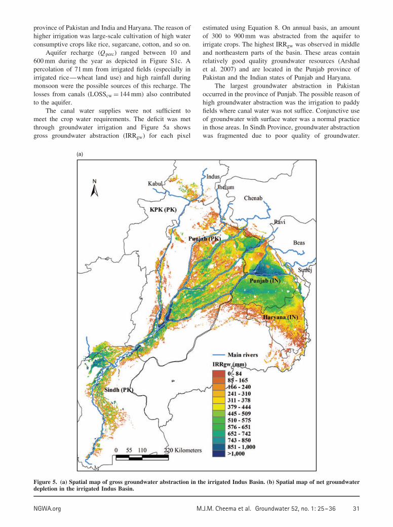
province of Pakistan and India and Haryana. The reason ofhigher irrigation was large-scale cultivation of high waterconsumptive crops like rice, sugarcane, cotton, and so on.

Aquifer recharge (Qperc) ranged between 10 and600 mm during the year as depicted in Figure S1c. Apercolation of 71 mm from irrigated fields (especially inirrigated rice—wheat land use) and high rainfall duringmonsoon were the possible sources of this recharge. Thelosses from canals (LOSScw = 144 mm) also contributedto the aquifer.

The canal water supplies were not sufficient tomeet the crop water requirements. The deficit was metthrough groundwater irrigation and Figure 5a showsgross groundwater abstraction (IRRgw) for each pixel

estimated using Equation 8. On annual basis, an amountof 300 to 900 mm was abstracted from the aquifer toirrigate crops. The highest IRRgw was observed in middleand northeastern parts of the basin. These areas containrelatively good quality groundwater resources (Arshadet al. 2007) and are located in the Punjab province ofPakistan and the Indian states of Punjab and Haryana.

The largest groundwater abstraction in Pakistanoccurred in the province of Punjab. The possible reason ofhigh groundwater abstraction was the irrigation to paddyfields where canal water was not suffice. Conjunctive useof groundwater with surface water was a normal practicein those areas. In Sindh Province, groundwater abstractionwas fragmented due to poor quality of groundwater.

(a)

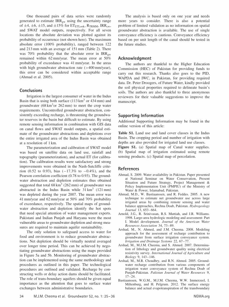
Figure 5. (a) Spatial map of gross groundwater abstraction in the irrigated Indus Basin. (b) Spatial map of net groundwaterdepletion in the irrigated Indus Basin.


(b)

Figure 5. Continued.

However, groundwater recharge by percolation from fieldsand canals resulted in conjunctive use of groundwater andsurface water in the northern Sindh Province (Siebert et al.2010).

Indian states of Punjab and Haryana were alsovulnerable to extensive groundwater pumping. The valueranged between 400 and 900 mm. Irrigated rice, wheatrotation was the dominant land use that required extensiveirrigation to meet crop water demand. The surfacewater supplies were not sufficient to meet the needtherefore the deficit was met through groundwater. Largenumber of small capacity tubewells was installed to pumpgroundwater. According to Shankar et al. (2011), tubewelldensity in the Punjab and Haryana states was 27 and 14.1

tubewells/km2 in 2001 and the number is increasing. Theflow rates may vary from 5 to 15 l/s.

The total irrigation supplies in the irrigated areas ofthe Indus Basin were estimated at 181 km3, an amountof 68 km3 originated from groundwater, while the surfacewater contribution was 113 km3. This diagnosis suggeststhat groundwater supplies 68/181 or 38% of the total waterapplied at the farm gate. The results are in agreementwith the 40% to 50% groundwater contribution reportedby Sarwar and Eggers (2006).

The gross groundwater abstraction can be exploredfurther to quantify the aquifer depletion (Figure 5b). Thetotal depletion of 31 km3 (121 mm/year) in the aquiferwas computed from IRRgw and the return flow Qgw. The


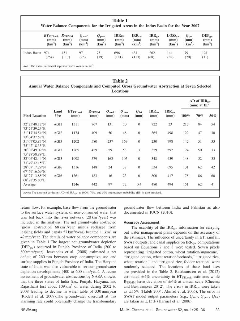
Table 1Water Balance Components for the Irrigated Areas in the Indus Basin for the Year 2007

ET ETLook(mm)(km3)

RTRMM(mm)(km3)

Q surf(mm)(km3)

Qperc(mm)(km3)

IRRRS(mm)(km3)

IRRcw(mm)(km3)

IRRgw(mm)(km3)

LOSScw(mm)(km3)

Qgw(mm)(km3)

DEPgw(mm)(km3)

Indus Basin 974(254)

451(117)

97(25)

75(19)

696(181)

434(113)

262(68)

144(38)

79(20)

121(31)

Note: The values in bracket represent water volume in km3.

Table 2Annual Water Balance Components and Computed Gross Groundwater Abstraction at Seven Selected

Locations

AD of IRRgw(mm) at EP

Pixel LocationLandUse

ETETLook(mm)

RTRMM(mm)

Q surf(mm)

Qperc(mm)

Q lat(mm)

IRRcw(mm)

IRRgw(mm) 100% 70% 50%

32◦25′48.12′′N73◦24′39.23′′E

AGI1 1311 767 131 70 0 722 23 213 84 54

31◦17′34.54′′N73◦04′37.52′′E

AGI2 1174 409 50 48 0 365 498 122 47 30

31◦07′05.83′′N75◦42′18.35′′E

AGI3 1202 580 237 169 0 230 798 142 51 33

30◦08′49.02′′N75◦28′58.89′′E

AGI3 1265 429 59 53 3 359 592 124 50 33

32◦06′42.44′′N73◦49′32.15′′E

AGI3 1098 579 163 105 0 348 439 148 52 35

28◦07′17.29′′N67◦59′16.69′′E

AGI6 1316 148 24 37 0 534 695 131 62 42

28◦27′13.85′′N68◦28′35.80′′E

AGI6 1361 183 16 23 0 800 417 175 86 60

Average 1246 442 97 72 0.4 480 494 151 62 41

Notes: The absolute deviation (AD) of IRRgw at 100%, 70%, and 50% exceedance probability (EP) is also provided.

return flow, for example, base flow from the groundwaterto the surface water system, of non-consumed water thatwas fed back into the river network (20 km3/year) wasincluded in the analysis. The net groundwater abstracted(gross abstraction 68 km3/year minus recharge fromleaking fields and canals 57 km3/year) became 11 km3 or42 mm/year. The details of water balance components aregiven in Table 1.The largest net groundwater depletion(DEPgw) occurred in Punjab Province of India (200 to800 mm/year). Jeevandas et al. (2008) estimated a netdeficit of 260 mm between crop consumptive use andsurface supplies in Punjab Province of India. The Haryanastate of India was also vulnerable to serious groundwaterdepletion developments (400 to 600 mm/year). A recentassessment of groundwater abstractions by NASA showedthat the three states of India (i.e., Punjab, Haryana, andRajasthan) lost about 109 km3 of water during 2002 to2008 leading to decline in water table of 330 mm/year(Rodell et al. 2009).The groundwater overdraft at thisalarming rate could potentially change the transboundary

groundwater flow between India and Pakistan as alsodocumented in IUCN (2010).

Accuracy AssessmentThe usability of the IRRgw information for carrying

out water management plans depends on the accuracy ofthe estimates. The influence of uncertainty in ET, rainfall,SWAT outputs, and canal supplies on IRRgw computationsbased on Equations 7 and 8 were tested. Seven pixelsrepresenting “irrigated cotton, wheat rotation/sugarcane,”“irrigated cotton, wheat rotation/orchards,” “irrigated rice,wheat rotation,” and “irrigated rice, fodder rotation” wererandomly selected. The locations of these land usesare provided in the Table 2. Bastiaanssen et al. (2012)estimated ±4% uncertainty in ETETLook estimates whileRTRMM have deviation of ±6% at annual scale (Cheemaand Bastiaanssen 2012). The errors in IRRcw were takenas ±15% (Habib 2004; Ahmad et al. 2005). The error inSWAT model output parameters (e.g., Q surf, Qperc, Q lat)are taken as ±15% (Harmel et al. 2006).


One thousand pairs of data series were randomlygenerated to estimate IRRgw using the uncertainty rangeof ±4, ±6, ±15, and ±15% for ETETLook, RTRMM, IRRcw,and SWAT model outputs, respectively. For all sevenlocations the absolute deviation was plotted against itsprobability of occurrence (not shown here). The maximumabsolute error (100% probability), ranged between 122and 213 mm with an average of 151 mm (Table 2). Therewas 70% probability that the absolute error in IRRgw

remained within 62 mm/year. The mean error at 50%probability of exceedance was 41 mm/year. In the areaswith high groundwater abstraction rate (>400 mm/year),this error can be considered within acceptable range(Ahmad et al. 2005).

ConclusionsIrrigation is the largest consumer of water in the Indus

Basin that is using both surface (113 km3 or 434 mm) andgroundwater (68 km3or 262 mm) to meet the crop waterrequirements. Uncontrolled groundwater abstraction, con-sistently exceeding recharge, is threatening the groundwa-ter reserves in the basin but difficult to estimate. By usingremote sensing information in combination with GIS dataon canal flows and SWAT model outputs, a spatial esti-mate of the groundwater abstractions and depletions overthe entire irrigated area of the Indus Basin was obtainedat a resolution of 1 km.

The parameterization and calibration of SWAT modelwas based on satellite data on land use, rainfall andtopography (parameterization), and actual ET (for calibra-tion). The calibration results were satisfactory and strongimprovements were obtained in the Nash-Sutcliffe crite-rion (0.52 to 0.93), bias (−17.3% to −0.4%), and thePearson correlation coefficient (0.78 to 0.93). The ground-water abstraction and depletion estimates thus obtainedsuggested that total 68 km3 (262 mm) of groundwater wasabstracted in the Indus Basin while 31 km3 (121 mm)was depleted during the year 2007. The mean error was41 mm/year and 62 mm/year at 50% and 70% probabilityof exceedance, respectively. The spatial maps of ground-water abstraction and depletion identify the hot spotsthat need special attention of water management experts.Pakistani and Indian Punjab and Haryana were the mostvulnerable areas to groundwater depletion and strong mea-sures are required to maintain aquifer sustainability.

The only solution to safeguard access to water forfood and environment is to reduce groundwater abstrac-tions. Net depletion should be virtually neutral averagedover longer time period. This can be achieved by nego-tiating groundwater abstractions using the maps providedin Figure 5a and 5b. Monitoring of groundwater abstrac-tion can be implemented using the same methodology andprocedures as outlined in this paper. The technologicalprocedures are outlined and validated. Recharge by con-structing wells or delay action dams should be facilitated.The role of trans-boundary aquifers should be given equalimportance as the attention that goes to surface waterexchanges between administrative boundaries.

The analysis is based only on one year and needsmore years to consider. There is also a potentialproblem of limited validation as no information on spatialgroundwater abstraction is available. The use of singleconveyance efficiency is cautious. Conveyance efficiencybased on per unit length of the canal should be tested inthe future studies.

AcknowledgmentThe authors are thankful to the Higher Education

Commission (HEC) of Pakistan for providing funds tocarry out this research. Thanks also goes to the PID,WAPDA and IWC, in Pakistan, for providing requireddata. Dr. Peter Droogers, of Future Water, kindly providedthe soil physical properties required to delineate basin’ssoils. The authors are also thankful to three anonymousreviewers for their valuable suggestions to improve themanuscript.

Supporting InformationAdditional Supporting Information may be found in theonline version of this article:

Table S1. Land use and land cover classes in the IndusBasin. The cropping period and number of irrigation withdepths are also provided for irrigated land use classes.Figure S1. (a) Spatial map of Canal water supplies.(b) Spatial map of irrigation estimated using remotesensing products. (c) Spatial map of percolation.

ReferencesAhmad, S. 2009. Water availability in Pakistan. Paper presented

at National Seminar on Water Conservation, PresentSituation and Future Strategy, Project Management &Policy Implementation Unit (PMPIU) of the Ministry ofWater & Power, Islamabad, Pakistan.

Ahmad, M.D., W. Bastiaanssen, and R. Feddes. 2005. A newtechnique to estimate net groundwater use across largeirrigated areas by combining remote sensing and waterbalance approaches, Rechna Doab, Pakistan. HydrogeologyJournal 13, 653–664.

Arnold, J.G., R. Srinivasan, R.S. Muttiah, and J.R. Williams.1998. Large-area hydrologic modeling and assessment: PartI. Model development. Journal of the American WaterResources Association 34, 73–89.

Arshad, M., N. Ahmed, and J.M. Cheema. 2008. Modelingapproach for the assessment of recharge contribution togroundwater from surface irrigation conveyance system.Irrigation and Drainage Systems 22, 67–77.

Arshad, M., M.J.M. Cheema, and S. Ahmed. 2007. Determina-tion of lithology and groundwater quality using electricalresistivity survey. International Journal of Agriculture andBiology 9, 143–146.

Arshad, M., M.R. Choudhry, and R.N. Ahmed. 2005. Ground-water recharge contribution from various components ofirrigation water conveyance system of Rechna Doab ofPunjab-Pakistan. Pakistan Journal of Water Resources 9,17–24.

Bastiaanssen, W.G.M., M.J.M. Cheema, W.W. Immerzeel, I.Miltenburg, and H. Pelgrum. 2012. The surface energybalance and actual evapotranspiration of the transboundary


Indus Basin estimated from satellite measurements and theETLook model. Water Resources Research 48, W11512.

Bastiaanssen, W.G.M., D.J. Molden, S. Thiruvengadachari,A.A.M.F.R. Smit, L. Mutuwatte, G. Jayasinghe. 1999.Remote sensing and hydrologic models for performanceassessment in Sirsa irrigation circle, India. Research Report27. International Water Management Institute, Colombo, SriLanka.

Beven, K. 2006. A manifesto for the equifinality thesis. Journalof Hydrology 320, 18–36.

Beven, K.J., and J. Freer. 2001. Equifinality, data assimilation,and uncertainty estimation in mechanistic modelling ofcomplex environmental systems. Journal of Hydrology 249,11–29.

Cheema, M.J.M., and W.G.M. Bastiaanssen. 2010. Land useand land cover classification in the irrigated Indus Basinusing growth phenology information from satellite datato support water management analysis. Agricultural WaterManagement 97, 1541–1552.

Cheema, M.J.M., and W.G.M. Bastiaanssen. 2012. Localcalibration of remotely sensed rainfall from the TRMMsatellite for different periods and spatial scales in theIndus Basin. International Journal of Remote Sensing 33,2603–2627.

Droogers, P. 2006. Unpublished data on pedo-transfer functions.Wageningen, The Netherlands, Future Water.

FAO. 1995. FAO-UNESCO digital soil map of the world andderived soil properties . Paris: UNESCO.

Foster, S.S.D., and P.J. Chilton. 2003. Groundwater: Theprocesses and global significance of aquifer degradation.Philosophical Transactions of the Royal Society of London.Series B: Biological Sciences 358, 1957–1972.

Githui, F., B. Selle, and T. Thayalakumaran. 2012. Rechargeestimation using remotely sensed evapotranspiration in anirrigated catchment in southeast Australia. HydrologicalProcesses . 26, 1379–1389.

Habib, Z. 2004. Scope for reallocation of river waters foragriculture in the Indus Basin. PhD dissertation. ENGREF,Montpellier, France.

Harmel, R.D., R.J. Cooper, R.M. Slade, R.L. Haney, andJ.G. Arnold. 2006. Cumulative uncertainty in measuredstreamflow and water quality data for small watersheds.Transactions of the ASABE 49, 689–701.

Healy, R., and P. Cook. 2002. Using groundwater levels toestimate recharge. Hydrogeology Journal 10, 91–109.

Hoffmann, L., A. El Idrissi, L. Pfister, B. Hingray, F. Guex,A. Musy, J. Humbert, G. Drogue, and T. Leviandier.2004. Development of regionalized hydrological models inan area with short hydrological observation series. RiverResearch and Applications 20, 243–254.

Huffman, G.J., R.F. Adler, D.T. Bolvin, G. Gu, E.J. Nelkin, K.P.Bowman, Y. Hong, E.F. Stocker, and D.B. Wolff. 2007. TheTRMM multisatellite precipitation analysis (TMPA): quasi-global, multiyear, combined-sensor precipitation estimatesat fine scales. Journal of Hydrometeorology 8, 38–55.

Immerzeel, W.W., and P. Droogers. 2008. Calibration of a dis-tributed hydrological model based on satellite evapotran-spiration. Journal of Hydrology 349, 411–424.

Immerzeel, W.W., A. Gaur, and S.J. Zwart. 2008. Integratingremote sensing and a process-based hydrological modelto evaluate water use and productivity in a south Indiancatchment. Agricultural Water Management 95, 11–24.

IUCN. 2010. Beyond Indus Water Treaty: Ground Water andEnvironmental Management—Policy Issues and Options .Karachi, Pakistan, IUCN.

Jeevandas, A., R.P. Singh, and R. Kumar. 2008. Concerns ofgroundwater depletion and irrigation efficiency in Punjabagriculture: A micro-level study. Agricultural EconomicsResearch Review 21, 191–199.

Kannan, N., J. Jeong, and R. Srinivasan. 2011. Hydrologicmodeling of a canal irrigated agricultural watershed with

irrigation best management practices: A case study. Journalof Hydrologic Engineering 16, 746–758.

Kreutzmann, H. 2011. Scarcity within opulence: Water man-agement in the Karakoram Mountains revisited. Journal ofMountain Science 8, 525–534.

Kroes, J.G., P. Droogers, R. Kumar, W.W. Immerzeel, R.S.Khatri, A. Roelevink, H.W. ter Maat, D.S. Dabas. 2003.A regional approach to model water productivity. In WaterProductivity of Irrigated Crops in Sirsa District, India.Integration of Remote Sensing, Crop and Soil Models andGeographical Information Systems , eds. J.C. Van Dam andR.S. Malik, 101–119. WATPRO Final Report.

Maupin, M.A. 1999. Methods to determine pumped irrigation-water withdrawals from the Snake River between upperSalmon Falls and Swan Falls dams, Idaho, using elec-trical power data,1990–95. U.S. Geological SurveyWater-Resources Investigation Report 99-4175. Littleton,Colorado: USGS.

Monteith, J.L. 1965. Evaporation and environment. Symposia ofthe Society for Experimental Biology 19, 205–234.

Nash, J.E., and J.V. Sutcliffe. 1970. River flow forecastingthrough conceptual models part 1—A discussion ofprinciples. Journal of Hydrology 10, 282–290.

Neitsch, S.L., J.G. Arnold, J.R. Kiniry, and J.R. Williams. 2005.Soil and Water Assessment Tool—Theoretical documenta-tion. Version 2005. Temple, Texas: Blackland Research &Extension Center.

PARC. 1982. Consumptive use of water for crops in Pakistan.Final Technical Report, 20–30. Pakistan AgriculturalResearch Council, Islamabad, Pakistan.

Qureshi, A.S., T. Shah, and M. Akhtar. 2003. The groundwatereconomy of Pakistan. Working Paper 64. Lahore, Pakistan:International Water Management Institute.

Rodell, M., I. Velicogna, and J.S. Famiglietti. 2009. Satellite-based estimates of groundwater depletion in India. Nature460, 999–1002.

Sarwar, A., and H. Eggers. 2006. Development of a conjunctiveuse model to evaluate alternative management options forsurface and groundwater resources. Hydrogeology Journal14, 1676–1687.

Scott, C.A., and T. Shah. 2004. Groundwater overdraft reductionthrough agricultural energy policy: Insights from Indiaand Mexico. International Journal of Water ResourcesDevelopment 20, 149–164.

Shah, T., J. Bruke, K. Vullholth, M. Angelica, E. Custodio,F. Daibes, J.D. Hoogesteger Van Dijk, M. Giordano, J.Girman, E. Kendy, J. Kijne, R. Llamas, M. Masiyandama,J. Margat, L. Marin, J. Peck, S. Rozelle, B. Sharma,L.F. Vincent, and J. Wang. 2007. Groundwater: A globalassessment of scale and significance. In Water for Food:Water for Life. A Comprehensive Assessment of WaterManagement in Agriculture, ed. D. Molden, 395–423.London, UK, Colombo, Sri Lanka: IWMI, Earthscan.

Shah, T., D.J. Molden, R. Sakthivadivel, and D. Seckler. 2000.The Global Groundwater Situation: Overview of Opportu-nities and Challenges . Colombo, Sri Lanka: InternationalWater Management Institute.

Shankar, P.S.V., H. Kulkarni, and S. Krishnan. 2011. India’sgroundwater challenge and the way forward. Economic andPolitical Weekly XLVI, 37–45.

Siebert, S., J. Burke, J.M. Faures, K. Frenken, J. Hoogeveen,P. Doll, and F.T. Portmann. 2010. Groundwater usefor irrigation—A global inventory. Hydrology and EarthSystem Sciences 14, 1863–1880.

Sivapalan, M., K. Takeuchi, S.W. Franks, V.K. Gupta, H.Karambiri, V. Lakshmi, X. Liang, J.J. McDonnell, E.M.Mendiondo, P.E. O’Connell, T. Oki, J.W. Pomeroy, D.Schertzer, S. Uhlenbrook, and E. Zehe. 2003. IAHS Decadeon Predictions in Ungauged Basins (PUB), 2003–2012:Shaping an exciting future for the hydrological sciences.Hydrological Sciences Journal 48, 857–880.


Srinivasan, R., T.S. Ramanarayanan, J.G. Arnold, and S.T.Bednarz. 1998. Large area hydrologic modeling andassessment: Part II. Model application. Journal of theAmerican Water Resources Association 34, 91–101.

Srinivasan, R., X. Zhang, and J. Arnold. 2010. SWAT ungauged:hydrological budget and crop yield predictions in the UpperMississippi River Basin. Transactions of the ASABE 53,1533–1546.

Thornton, P.E., S.W. Running, and M.A. White. 1997. Generat-ing surfaces of daily meteorological variables over largeregions of complex terrain. Journal of Hydrology 190,214–251.

Zhang, X., R. Srinivasan, and M.V. Liew. 2008. Multi-sitecalibration of the SWAT model for hydrologic modeling.Transactions of the ASABE 51, 2039–2049.


Spatial Quantification of Groundwater Abstraction in the ... Quantiﬁcation of Groundwater...

Documents

Transcript of Spatial Quantification of Groundwater Abstraction in the ... Quantiﬁcation of Groundwater...