Spatial OppositesSpatial Opposites

M. KubovyVirginia University, USAVirginia University, USA

U. Savardi Verona University, ItalyVerona University, Italy

I. Bianchi Macerata University, ItalyMacerata University, Italy

Spatial Opposites

The study of opposites as a cognitive structure has been more or less exhausted in contemporary psychology, within the study of pairs of antonyms (Croft & Cruse, 2004; Cruse, 1986, 2000; Fellbaum, 1998; Jones, 2002; Lyons, 1977; Muehleisen, 1997; Murphy, 2003; Willners, 2001).

-Gradable opposites (e.g. large/small), defined as qualities that can be conceived of as 'more or less' (e.g. fairly large, very large); the scale or dimension associated has a mid interval (e.g. if something is neither large nor small, it is medium size);

-Complementary opposites (e.g. dead/alive) characterized by the fact they divide a conceptual domain into two mutually exclusive compartments, so that “what does not fall into one of the compartments must necessarily fall into the other" (Cruse 1986, p. 198; see also Palmer, 1976; Carter, 1987; Jackson, 1988). These are sometimes called contradictory or simple binary opposites (Kempson, 1976);

- Reversive opposites (Lehrer & Lehrer, 1982, Egan, 1968): “adjectives or adverbs which signify a quality or verbs or nouns which signify an act or state that reverse or undo the quality, act, or state of the other” (Egan 1968, 27a). E.g. tie/untie, enter/leave.

Different classifications have been proposed:

- Directional opposites (Lyons, 1977; Cruse, 1986): pairs such as in/out or clockwise/anticlockwise, which are related to opposite directions on a common axis.

- Relational (Cruse 1986; Palmer, 1976; Leech 1974) or relative (Egan 1968) or conversive opposites (Lyons 1977): pairs which imply a relationship where one of them cannot be used without suggesting the other, such as parent/child and teacher/student.

Cruse (1986) also proposed defining two further classes of “near opposites”:

- "impure" opposites, i.e. opposites which include a more elementary opposition within their meaning: “Giant:dwarf can be said to encapsulate the opposition between large and small (but this opposition does not exhaust their meaning); likewise, shout and whisper encapsulate loud and soft, criticize and praise encapsulate good and bad..." (Cruse 1986, p. 198);

- pairs that are only weakly contrasted because of "the difficulty in establishing what the relevant dimension or axis is" (Cruse 1986, p.262). E.g. work/play, town/country.

• OBSERVATION 1: In these classifications, structural criteria (see the distinction between gradable and complementary opposites) coexist with semantic (e.g. reversive opposites, impure opposites) pragmatic (e.g. weakly contrasted opposites) and even logical (e.g. relational opposites) criteria.

• OBSERVATION 2: Despite the fact that very specialized taxonomies have been developed, this high level of descriptive specialization leaves researchers with too many questions when confronted with the everyday use of opposites. And this seems to be the cause of the recent need to look afresh at the cognitive structure of ‘opposites’, moving towards new approaches in semantics (Muehleisen, 1997; Jones, 2002), linguistics (Paradis & Willners, 2006) and even in brain sciences (Kelso & Engstrom, 2006).

Our goal:

We propose a new approach to the study of the “internal structure of

opposites” based on what Kubovy (2002) called phenomenological

psychophysics. (This could go beyond the simplistic distinction between

gradable and complementary opposites).

Our methods “are phenomenological: they rely on the reports of observers

about their phenomenal experiences. They are also psychophysical: they

involve systematic exploration of stimulus spaces and quantitative

representation of perceptual responses to variations in stimulus

parameters.” (Kubovy and Gepshtein, 2003, p. 45).

the structure of opposites can be defined metrically and topologically, based on direct estimates and descriptions of the characteristics of three components: the two poles and the intermediates.

Why using spatial opposites?

Since our intuition is that the analysis of the cognitive structure of contraries that we propose is grounded in perception. Since perception of space is recognized to be almost exclusively the result of automatic processes, we considered space a suitable domain to start with.

General Hypothesis:

Study 1: A Metrical analysis

Goal: to determine how observers think we should partition an interval () into two regions: one to which a property () applies and a complementary region to which the opposite property () applies.

E.g.: it is likely that we think that the scope of large things is greater than the scope of small things. Therefore, the interval between small and large (see Figure) should be partitioned into two unequal intervals, and ¯.

We do not mean that we encounter more large than small objects in an everyday environment. Nor do we mean that we encounter more types of large objects than small ones.

The question is rather how to put these objects or types of objects into a finite number of bins ( -experience bins).

The problem is closely related to the statistical problem of determining how to assign continuous data to bins in a histogram.

-experience bins

Consider two ants: one large, the other small. Since you can readily tell that one is bigger than the other you would say that they differ in size.

If, however, you were asked whether there was a qualitative size-difference between them, taking into account the range of all object sizes, from the smallest thing you can see (say, a grain of sand) to the biggest thing you can see (perhaps a tall and wide rock wall that exceeds your visual field), you might choose to place them in the same size-experience bin. On the other hand, you might decide that because there is a qualitative size-difference between the size of ants and the size of butterflies or nuts, they belong in different size-experience bins, whereas you might assign butterflies and nuts to the same size-experience bin.

Once the concept of -experience bins is clear, it is not difficult to take the next step which is to estimate the number of -experience bins referring to one property, to the opposite property, and to the properties perceived as intermediates.

Method

• Participants: 45 undergraduates (Industrial Design at the University of Milan) randomly assigned to ten groups of four and one group of five).

• Procedure: Each group was given a sheet of 37 labelled scales. Each scale consisted of two stacked bars. The distance between the end-points (10 cm), represented the whole range of variations in between the two poles. They were asked:

1. to draw a vertical boundary between opposites in the upper bar, in order to express the proportion referring to one property (-bins) and the proportion referring to the opposite property (¯-bins).

2. to draw in the lower bar two vertical boundaries, on either side of the boundary drawn in the upper bar, to indicate the range of -experiences that are neither nor ¯.

Results:

From the responses we computed the data in Table 1.

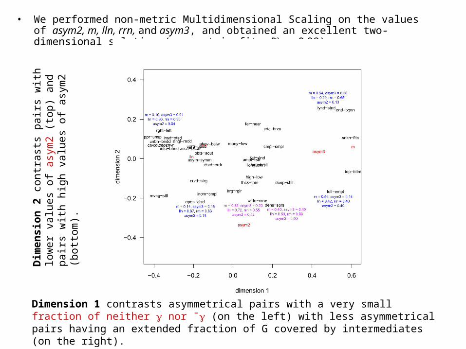
• We performed non-metric Multidimensional Scaling on the values of asym2, m, lln, rrn, and asym3, and obtained an excellent two-dimensional solution (non-metric fit, R2 = 0.99)

Dimension 1 contrasts asymmetrical pairs with a very small fraction of neither nor ¯ (on the left) with less asymmetrical pairs having an extended fraction of G covered by intermediates (on the right).

Dim

en

sio

n 2

contr

ast

s pair

s w

ith low

er

valu

es

of

asy

m2

(to

p)

and p

air

s w

ith

hig

h v

alu

es

of

asy

m2

(bott

om

).

Study 2: A topological analysis

From the results from study 1 it is not possible to recognize further differences between the pairs that may remain hidden behind the proportional indexes used.

For example, dense–sparse and wide–narrow are close in study 1.

However, to be maximally dense (e.g., a set of dots; passengers on a bus) means that when the elements are packed as densely as possible, adding dots will not change the texture—we have reached a saturation point (in topology this is called a closed interval). This is not the case for wide: we can perceive a road as being very wide, but there is no maximum width (in topology this is called an open interval). A point, in topology, is treated as a degenerate interval. This captures the structures of properties consisting of a single experience-bin (like closed, or still).

Method

Participants: 54 undergraduates (Industrial design at the University of Milan), divided in 18 groups of 3.

Procedure: The 37 spatial pairs were randomly presented in a table.

Participants were asked to make the following distinctions:

a) for the two poles, the distinction between single experiences (point, P) and ranges of experiences (intervals) and, in the latter case, between closed intervals (i.e. having a “final state”, showing the property at the maximum possible degree) and open intervals (i.e. where this “final” state is not identifiable);

b) for the intermediates, the distinction between the existence or non–existence of properties which are “neither one pole nor the other”. If these properties existed, participants were then asked to distinguish between single experiences (P) and intervals (I).

Results

We performed a Correspondence Analysis on the frequency table of the 37 pairs x 24 series of triples. This produced a two-dimensional solution.

If we divide the map into four quadrants, we note that:

- the n pairs fall in quadrant II (upper left)

- the p pairs straddle the boundary between quadrants I and IV,

- the r pairs form a rough diagonal line running from quadrant I to III.

n

pr

Joint Analysis

In order to describe the pairs both metrically and topologically, we took the four pairs of coordinates obtained in Studies 1 (nmMDS) and 2 (CA), and submitted them to nmMDS (fig. on the left) and hierarchical clustering (Fig. on the right).

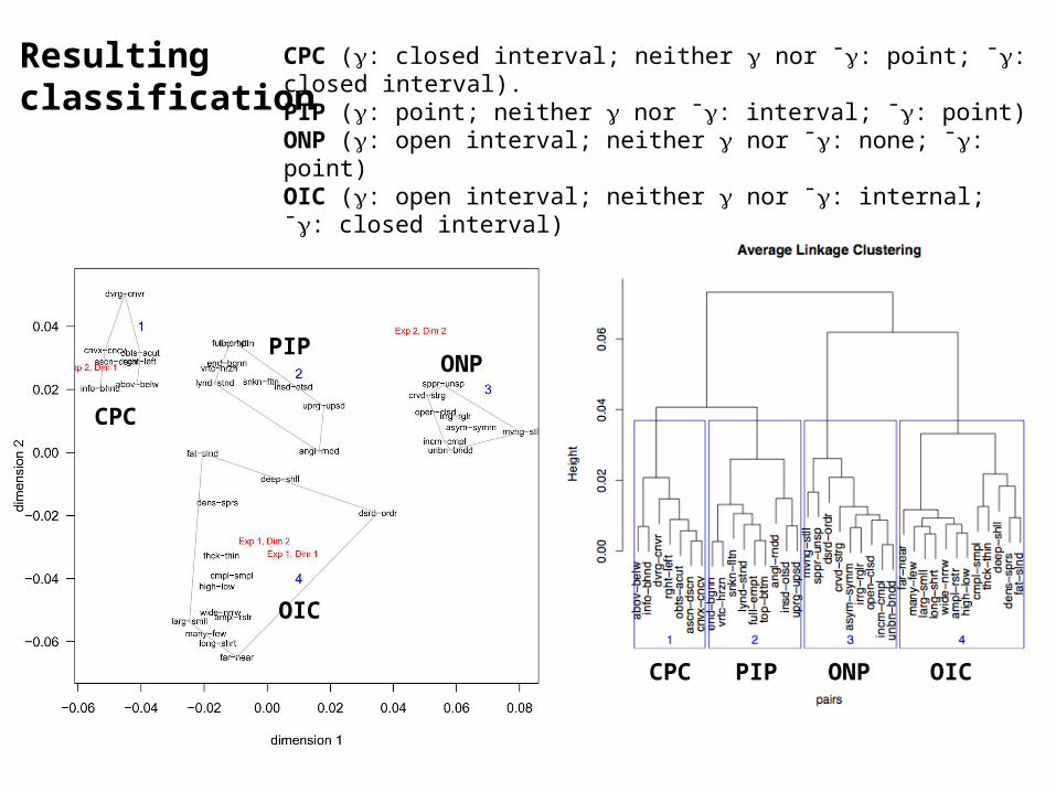
Resulting classification

CPC (: closed interval; neither nor ¯: point; ¯: closed interval).PIP (: point; neither nor ¯: interval; ¯: point) ONP (: open interval; neither nor ¯: none; ¯: point) OIC (: open interval; neither nor ¯: internal; ¯: closed interval)

CPC

CPC

PIP

PIP

ONP

ONP

OIC

OIC

Conclusions

• The studies presented have shown that the proportional extension of the two poles and the intermediates can be defined by participants with high accuracy, and that accurate metrical classifications can be identified.

• These metrical classifications are further enriched when considering topological aspects regarding the nature of the three components making up each pair.

• The combination of both metrical and topological aspects lead to a new system of classification.

We consider that the approach which was applied to the case of spatial opposites may be extended to the study of the opposites in whatever domain.

We are aware that a systematic validation of these spatial structures in different groups of languages is necessary. We are however inclined to expect that these structures will be for the most part generalized, if they describe, as we believe, the result of perceptual and cognitive processes that are somehow pre-linguistic.