Spatial Normalization of Human Back Images

for Dermatological Studies

H. Mirzaalian1,3, G. Hamarneh1, T. K. Lee2,3

1Medical Image Analysis Lab at the School of Computing Science, Simon FraserUniversity, BC, Canada, 2 Cancer Control Research, BC Cancer Agency, BC Canada,3Photomedicine Institute, Department of Dermatology and Skin Science University of

British Columbia, and Vancouver Coastal Health Research Institute, BC, Canada

Abstract. Density of pigmented skin lesions (PSL) is a strong predic-tor of malignant melanoma. Some dermatologists advocate periodic full-body scan for high-risk patients. It is clinically important to compareand detect changes in the number and appearance of PSL across time.However, manual inspection and matching of PSL is tedious, error-prone,and suffers from inter-rater variability. Therefore, an automatic methodfor tracking corresponding PSL would have significant health benefits.In order to automate the tracking of PSL in human back images, wemust perform spatial normalization of the coordinates of each PSL, asis done in brain atlases. We propose the first human back template (at-las) to obtain this normalization. Four pairs of anatomically meaningfullandmarks (neck, shoulder, armpit and hip points) are used as referencepoints on the skin-back image. Using the landmarks, a grid with longi-tudes and latitudes is constructed and overlaid on each subject specificback image. To perform spatial normalization, the grid is registered intothe skin-back template, a unit-square rectilinear grid. We demonstratethe benefits of our approach, on 56 pairs of real dermatological images,through the increased accuracy of PSL matching algorithms when ouranatomy-based normalized coordinates are used.

1 Introduction

Melanoma is one of the fastest growing cancers among the white population inthe world with an average 3% increase in incidence for the last four decades.In the USA and Canada alone, it was estimated that there will be 73,720 casesof melanoma in 2009 [2,3]. The mechanism of melanoma development is notfully understood. Nevertheless, pigmented skin lesions (PSL) density (numberof PSL per unit area of skin) have been reported as the strongest risk factor,with about 50% of melanoma originating from pre-existing PSL. Early diagno-sis of melanoma may lead to potentially life-saving therapy. To allow for earlydiagnosis, patients are full-body scanned periodically and digital color two di-mensional images of the skin are collected during the process. One example ofback images at two different times is shown in Figure 1. During a dermatologicalexamination, physicians compare the skin images at different time instances to

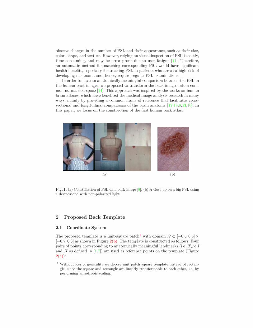
observe changes in the number of PSL and their appearance, such as their size,color, shape, and texture. However, relying on visual inspection of PSL is costly,time consuming, and may be error prone due to user fatigue [11]. Therefore,an automatic method for matching corresponding PSL would have significanthealth benefits, especially for tracking PSL in patients who are at a high risk ofdeveloping melanoma and, hence, require regular PSL examinations.

In order to have an anatomically meaningful comparison between the PSL inthe human back images, we proposed to transform the back images into a com-mon normalized space [14]. This approach was inspired by the works on humanbrain atlases, which have benefited the medical image analysis research in manyways; mainly by providing a common frame of reference that facilitates cross-sectional and longitudinal comparisons of the brain anatomy [17,18,8,13,10]. Inthis paper, we focus on the construction of the first human back atlas.

(a) (b)

Fig. 1: (a) Constellation of PSL on a back image [9], (b) A close up on a big PSL usinga dermoscope with non-polarized light.

2 Proposed Back Template

2.1 Coordinate System

The proposed template is a unit-square patch1 with domain Ω ⊂ [−0.5, 0.5] ×[−0.7, 0.3] as shown in Figure 2(b). The template is constructed as follows. Fourpairs of points corresponding to anatomically meaningful landmarks (i.e. Type I

and II as defined in [1,7]) are used as reference points on the template (Figure2(a)):

1 Without loss of generality we choose unit patch square template instead of rectan-gle, since the square and rectangle are linearly transformable to each other, i.e. byperforming anisotropic scaling.

i. The point where the left (right) side of the neck meets the left (right)shoulder, or neck-left nl (neck-right nr) for short, corresponds to Nl (Nr)in the normalized space of the template. Note that we use capital lettersfor template and small letters for image space coordinates.

ii. The point where the left (right) shoulder meets the left (right) arm,denoted by shoulder-left sl (shoulder-right sr), corresponds to Sl =(−0.5, 0.3) (Sr = (0.5, 0.3)) in the normalized space of the template.

iii. The left and right armpits (al and ar, respectively) correspond to Al =(−0.5, 0) and Ar = (0.5, 0) in the normalized space of the template,respectively.

iv. The left hip point (hl) and right hip point (hr) correspond to Hl =(−0.5,−0.7) and Hr = (0.5,−0.7) in the normalized space of the tem-plate, respectively.

According to the classification of the landmarks by Bookstein [1,7], Type

I landmark is defined as the discrete juxtapositions of tissues e.g. the pointwhere three structures meet, the branching point of the tree structures, or theintersections of extended curves with planes of symmetry. The armpit point isthe lateral intersection of left (right) arm and the backs left (right) silhouette andhence, can be classified as Type I. Landmark Type II is defined as the maximumof curvature or other local morphogenetic process. The neck and shoulder pointsare of this type.

Note that all the anatomical landmark locations in the template space (exceptNl and Nr) are at specific coordinates in the domain Ω (Figure 2(b)). Thesubject specific landmarks, on the other hand, can be any spatial coordinates inthe physical image space. The coordinate system of the template is formed bylongitudes and latitudes (Figure 2(b)).

The central latitude is a straight horizontal line segment AlAr which connectsAl and Ar, whereas the central longitude is the line segment NmHm connectingthe medial point Nm = (0, 0.3) with Hm = (0,−0.7) and passing through Sm =(0, 0.3) and Am = (0, 0), where the subscript m indicates the midpoint betweenthe corresponding left and right reference points, e.g. Nm = (Nl + Nr)/2. Thetopmost (superior) latitude SlSr, the bottommost (inferior) latitude HlHr, theleftmost longitude SlHl, and the rightmost longitude SrHr define the borders ofthe domain Ω of the template. Note that in the template space: AlAr⊥NmHm,SlHl ‖ NmHm ‖ SrHr and SlSr ‖ AlAr ‖ HlHr where ⊥ denotes perpendicularand ‖ denotes parallel. Finally, based on the anatomical landmarks and thereference central latitude and longitude, a template based rectilinear coordinatesystem is defined and a complete Cartesian grid is overlaid on the template.

nlsl

al

hl

nr

sr

ar

hr

(a) Landmark

−0.5 −0.4 −0.3 −0.2 −0.1 0 0.1 0.2 0.3 0.4 0.5

−0.6

−0.5

−0.4

−0.3

−0.2

−0.1

0

0.1

0.2

0.3

Sl

Al

Hl

Hm

Am

Nm

Sr

Ar

Hr

(b) Template

Fig. 2: Human back template. (a) Landmarks are shown in the image. (b) Templateof the back image. The red and green points correspond to the normalized coordinatesof the PSL and the reference anatomical landmarks, respectively. The vertical andhorizontal red lines correspond to the central longitude and latitude.

2.2 Spatial Normalization of Back Coordinates

At a high level, the spatial normalization is done by following these steps: de-tecting the basic longitudes and latitudes in the image space, constructing thegrid, and establishing a mapping between the continuous image space and thetemplate. The details are described below.

Detecting the Basic Longitudes and Latitudes To perform spatial nor-malization, a set of six basic latitudes (Superior, Central, and Inferior) andlongitudes (Left, Right and Central) is overlaid on each subject specific back im-age to register it into the template coordinate system (Figure 3). The latitudesand longitudes are constructed using the aforementioned anatomical landmarkpoints, some lateral edge points of the left and right silhouette of the back, andsuperior edge points of both shoulders’ silhouettes (Figure 3(a)). Note that, mostof the latitudes and longitudes in the image space are smooth curves fitted tothe anatomical landmarks and medial lines as explained below. Consequently,the grid in the image space is no longer rectilinear but rather curved. We nowprovide the details on how the latitudes and longitudes are constructed.

i. The Left (Right) longitude as shown in Figure 3(b) is a degree 3 poly-nomial least-squares fitted to the lateral edge points of the back’s left(right) silhouette and constrained to pass through al (ar). Least squarefitting calculates the polynomial coefficient such that the polynomialpasses as close as possible to the points, minimizing the square of theerror distance. We use a degree 3 polynomial because it provides suffi-cient degrees of freedom to model the sides without excessive inflectionpoints. Degree 2 is not flexible enough and higher degree than 3 would

increase the complexity in addition to over-fitting the curve to the noisein the detected edge points.

ii. The Central longitude (Figure 3(c)) is the medial curve between the leftand right longitudes and is calculated as follows: First, we calculate thedistance transform (DT ) between the Left and Right longitudes. Next,we calculate the gradient of the DT image: (DT ), which captures theamount by which the DT image changes along the vertical and hori-zontal directions. Finally, we construct the center longitude via a degree3 polynomial least-squares fitted to the local maxima of the gradientmagnitude of DT : |(DT )| (Figure 4). Alternatively, we can calculatethe center longitude as the loci of points midpoint between the Leftand Right longitudes (Figure 4). We obtained similar results using bothapproaches. The second definition, however, is preferable because its sim-pler to compute, whereas the first is more rigourous mathematically.

iii. Superior latitude (Figure 3(d)) is a degree 6 polynomial least-squaresfitted to the superior edge points of both shoulders’silhouettes. Degree6 is chosen to accommodate the number of concavities and convexitiesthat can occur along these superior edge points.

iv. Central latitude (Figure 3(e)) is a straight line segment alar connectingal to ar .

v. Inferior latitude (Figure 3(f)) is a straight line segment hlhr connectinghl and hr.

As a result, the image domain of a specific subject’s back, ω ⊂ R2, is boundedby the left and right longitudes and superior and inferior latitudes.

Constructing the Grid The intersections of the basic longitudes and latitudescan be considered as the control points for the mapping between two spaces. Asmore control points increase the precision of the mapping, we interpolate asmany additional longitudes and latitudes to achieve a desired accuracy. Thelines are interpolated between the basic longitudes and attitudes using equal arclength sampling points, which can be classified as Type III landmarks [1]. Figure3(g)-3(l) shows the steps of interpolating longitudes and latitudes of the grid

Mapping the Continuous Spaces After established the control points, weset up the correspondence between any point in the two continuous domains (notonly the landmarks, points on the latitudes and longitudes or their intersections)by warping the grid to the template. We evaluated two interpolation methods:Barycentric coordinates (BC) [6] and Thin plate splines (TPS) [5].

Barycentric Coordinates (BC) Method: The BC method can map pointsusing the following steps:

(a) (b) (c) (d)

(e) (f) (g) (h)

(i) (j) (k) (l)

Fig. 3: Different steps of the grid construction: (a) Points inserted by the user (blue arethe edge points, and red are the landmarks) (b) Left and Right longitudes, (c) Centrallongitude, (d) Superior latitude, (e) Central latitude, (f) Inferior latitude, (g) Equal arclength samplings , (h) Interpolating latitudes between superior and central latitudes,(i) Interpolating latitudes between central and inferior latitudes, (j) Interpolating lon-gitudes between left and central longitudes, (k) Interpolating longitudes between rightand central longitudes, (l)The grid overlaid on the back image.

i. For each point, p = (px, py) ∈ ω, find the cell cell(p) ⊂ ω containingp, i.e. cell(p) is the area enclosed between the two nearest longitudesand latitudes to p. As shown in Figure 5(a)-5(b), we locate the pointsa = (ax, ay), b = (bx, by), and c = (cx, cy).

ii. Find the corresponding cell CELL(P ) ⊂ Ω in the template domain.CELL(P ) is the area enclosed by the corresponding longitudes and lat-

(a) (b) (c) (d) (e)

Fig. 4: (a) Image contains the left and right longitudes. (b) Binary image contains theleft and right longitudes. (c) The distance transform of the image (b). (d) Points withmaximum gradient. (e) Red and blue curves show the central longitude resulted fromDT and average line between the left and right longitudes respectively. A close up ofthe small rectangular region near the neck is shown on the right.

itudes of the bounding cell(p) in the image domain. For example, welocate the control points A, B and C as shown in Figures 5(c)-5(d).

iii. Compute the BC coordinates (t1, t2, t3) of p using (1) [6].∣

∣

∣

∣

∣

∣

t1t2t3

∣

∣

∣

∣

∣

∣

=

∣

∣

∣

∣

∣

∣

ax bx cx

ay by cy

1 1 1

∣

∣

∣

∣

∣

∣

−1∣

∣

∣

∣

∣

∣

px

py

1

∣

∣

∣

∣

∣

∣

(1)

iv. The point P ⊂ Ω is determined by the same BC coordinates as P =t1A + t2B + t3C.

Thin Plate Splines (TPS) Method: TPS wraps points from one domain toanother domain by mimicking the deformation of a thin-plate and minimizes thebending energy. In particular, interpolated coordinates using TPS are given by[5]:

f(x, y) =

K∑

i=1

ciφ(|(x, y) − (xi, yi)|) + a10x + a01y + a00 (2)

where |.| denotes the usual Euclidian distance, (xi, yi) is a set of control points,aij and ci are warping coefficients representing the affine transformation andnon-affine deformations, respectively. φ is referred as the Kernel function of thethin plate spline and is given by φ = r2logr where r is the distance

√

x2 + y2.The kernel models elasticity and non-rigid transformation and govern the dis-placement of the control points.

Our control points are intersections of the longitudes and latitudes. TPS fitsa function f such that any point (xi, yi) ⊂ ω is mapped to (Xi, Yi) ⊂ Ω ((Xi, Yi):(Xi, Yi) = f(xi, yi)) by minimizing the following energy function [5]:

E =

∫ ∫

(Eb(x, y))2)dxdy (3)

where Eb(x, y) = (d2f

dx2 )2 + 2( d2f

dxdy)2 + (d2f

dy2 ) is a measure of the bending energy

at (x, y).

The result of these two alternative interpolation methods is to stablish abijective function f : ω → Ω mapping between points between two domains. Inthe BC method, curves bounding the cells are approximated by straight lineswhen establishing correspondence between the two continues domains. TPS doesnot rely on this assumption and hence it is more accurate. However, TPS is morecomputationally expensive than the BC. Using our database of back imagesdescribed in section 3, the difference between the normalized coordinates usingBC and TPS in the unit square patch is: |fBC(x, y) − fTPS(x, y)| = 2.3 ×10−5 ± 1.87 × 10−7, which shows that the increase in accuracy does not justifythe additional computational complexity of TPS.

Figure 6 demonstrates the mapping between the two spaces. Cells, longitudesand latitudes in the image and template space are colored with the same colors.

(a)

b

pc

a

(b)

−0.5 −0.4 −0.3 −0.2 −0.1 0 0.1 0.2 0.3 0.4 0.5

−0.6

−0.5

−0.4

−0.3

−0.2

−0.1

0

0.1

0.2

0.3

(c)

−0.45 −0.4 −0.35 −0.3 −0.25

0.1

0.15

0.2

0.25

0.3A

B C

P

(d)

Fig. 5: Interpolating points by Barycentric Coordinates: (a) Points in the image do-main. (b) Shows a close up of cell(p) which p ∈ cell(p). (c) Points in the templatedomain. (d) Shows a close up of CELL(P ) correspond to cell(p).

3 Back Images

The data used in this study were obtained from color slides taken from anepidemiologic study concerning the use of broad-spectrum sunscreen and PSLdevelopment. The images were digitized with 24-bit color at 2000 dpi, with afinal resolution of about 0.25 mm/pixel. A set of 56 pairs of digitized imagescontaining PSL was chosen to evaluate the proposed method. Each image pairbelongs to a single subject imaged at baseline and 3 years later. Ground truthidentification of all PSL, correspondence of the PSL across the pair of images, aswell as the anatomical landmarks were provided for images pairs by an expertuser [9].

(a) (b) (c)

−0.5 −0.4 −0.3 −0.2 −0.1 0 0.1 0.2 0.3 0.4 0.5

−0.6

−0.5

−0.4

−0.3

−0.2

−0.1

0

0.1

0.2

0.3

(d)

Fig. 6: Corresponding cells, longitudes and latitudes in the image and template domainare shown with the same color within the first and second rows respectively.

4 Experiment

Figure 7 shows four examples of the overlaid grids on the back images and thenormalized coordinates of the PSL resulting from our proposed template. Corre-sponding latitudes and longitudes on the image-template space are shown withthe same color. Our primary application of using normalized spatial coordinatesis to match PSL between two images captured at different times. In order toshow that utilizing normalized spatial coordinates improves the PSL matching,in [15], we compared the matching results of different algorithms with and with-out spatial normalization. The following matching algorithms were tested onthe 56 pairs of dermatological images: Coherent Point Drift (CPD) [16], shapecontexts (SC+TPS) [4], the spectral technique of (Spect) [12] and Hypergraphmatching (d = 2) (Hyp) [20]. Examples of finding corresponding PSL automati-cally in real image data are shown in Figure 8 (for further details, we refer thereader to [15]).

Figure 9 shows the number of incorrect matches (NIM) for the state of theart matching algorithms. Blue and red bars show the error results using imagespace coordinates (no spatial normalization) versus using normalized space co-ordinates (using the proposed template), respectively. As it can be seen, usingour proposed anatomy based normalized coordinates, we substantially improvedthe PSL matching accuracy for all algorithms.

5 Conclusions

An automatic method for matching PSL on human back images is of utmostimportance for early detection of potential malignancies. In order to have ananatomically meaningful comparison between PSL in the human back images,we need to perform spatial normalization. In this work, we propose the firsthuman back template to perform spatial normalization. The results show thatusing our proposed anatomy based normalized coordinates for the state of the

−0.5 −0.4 −0.3 −0.2 −0.1 0 0.1 0.2 0.3 0.4 0.5

−0.6

−0.5

−0.4

−0.3

−0.2

−0.1

0

0.1

0.2

0.3

−0.5 −0.4 −0.3 −0.2 −0.1 0 0.1 0.2 0.3 0.4 0.5

−0.6

−0.5

−0.4

−0.3

−0.2

−0.1

0

0.1

0.2

0.3

−0.5 −0.4 −0.3 −0.2 −0.1 0 0.1 0.2 0.3 0.4 0.5

−0.6

−0.5

−0.4

−0.3

−0.2

−0.1

0

0.1

0.2

0.3

−0.5 −0.4 −0.3 −0.2 −0.1 0 0.1 0.2 0.3 0.4 0.5

−0.6

−0.5

−0.4

−0.3

−0.2

−0.1

0

0.1

0.2

0.3

Fig. 7: Some example of the overlaid grid and the template. (a) The landmarks usedin constructing the grid. (b) The overlaid grid on the back images. (c) The resultingnormalized coordinates of the PSL using the proposed template. Corresponding lati-tudes and longitudes on the grid and the template are shown with the same color in(b-c). (d-e) Corresponding cells on the grid and the template are shown with the samecolor. Red points are correspond to the positions of the PSL.

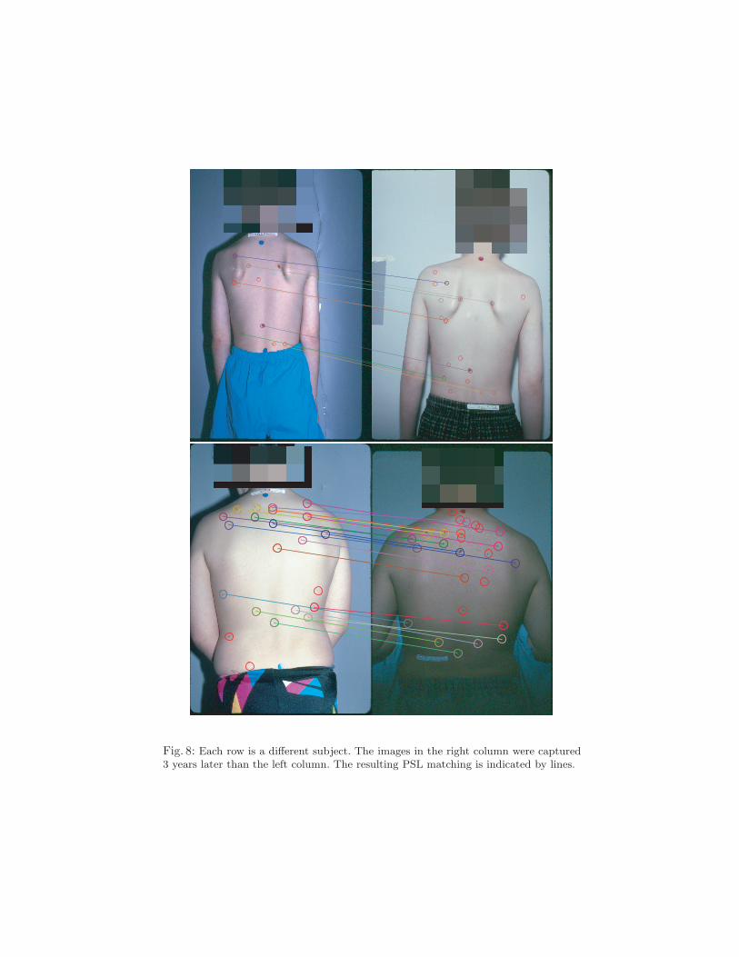
Fig. 8: Each row is a different subject. The images in the right column were captured3 years later than the left column. The resulting PSL matching is indicated by lines.

CPD Hyp ModifiedHypSC+TPS Vor Spect0

0.5

1

NIM

Fig. 9: PSL matching evaluation (using number of incorrect matches (NIM)) of differentmethods (along the horizontal axis) when spatial image coordinates (blue bars) ornormalized coordinates (red bars) are used in the matching. We note a substantialimprovement in accuracy when normalized coordinates are used.

art matching algorithms, we substantially improve the PSL matching accuracy.We do not claim that our template is the best possible template, so we plan tocontinue exploring alternative approaches to improve it and we anticipate othergroups will do too. One of the challenges, as observed in this study, will be todevelop a robust definition of the hip anatomical landmark, which we plan toaddress through discussions and consultations with dermatologists. We are alsoworking on automated image processing methods for identifying the PSL and theanatomical landmarks, which will complement our work on PSL matching [15]and spatial normalization presented in this paper, in order to produce an end-to-end system for reading pairs of human back images, counting the PSL, anddetecting appearing and disappearing PSL. Suspicious PSL are further analyzedusing shape and color and texture properties as in [19].

References

1. Morphometric Tools for Landmark Data. UK: Cambridge University Press, 1997.2, 3, 5

2. American cancer society (2009). cancer facts and figures 2009, american cancersociety. 2009. Atlanta, USA. 1

3. Canadian cancer societys steering committee (2009). canadian cancer statistics2009. 2009. Toronto, Canada. 1

4. S. Belongie, J. Malik, and J. Puzicha. Shape matching and object recognition usingshape contexts. IEEE PAMI, 24(4):509–522, 2002. 9

5. F. Bookstein. Principal warps: thin-plate splines and the decomposition of defor-mations. IEEE PAMI, 11(6):567–585, 1989. 5, 7

6. O. Bottema. On the area of a triangle in barycentric coordinates. 8:228–231, 1982.5, 7

7. T. Cootes, C. Taylor, D. Cooper, and J. Graham. Active shape models: Theirtraining and application. 61(1):38–59, 1995. 2, 3

8. A. Evans, M. Kamber, D. Collins, and D. MacDonald. An MRI-based probabilistic

atlas of neuroanatomy, chapter MRI-based probabilistic atlas of neuroanatomy,pages 263–274. Plenum Press, 1994. 2

9. R. Gallagher, J. Rivers, T. Lee, C. Bajdik, D. I. McLean, and A. Coldman.Broad-Spectrum Sunscreen Use and the Development of New Nevi in White Chil-

dren: A Randomized Controlled Trial. Journal of American Medical Association,283(22):2955–2960, 2000. 2, 8

10. D. Hill, P. Batchelor, M. Holden, and D. Hawkes. Medical image registration.Physics in medicine and biology, 46:R1–R45, 2001. 2

11. E. A. Holly, J. W. Kelly, S. N. Shpall, and S. H. Chiu. Number of melanocyticnevi as a major risk factor for malignant melanoma. J. Am. Acad. Dermatol,17:459–468, 1987. 2

12. M. Leordeanu and M. Hebert. A spectral technique for correspondence problemsusing pairwise constraints. IEEE ICCV, 2:1482–1489, 2005. 9

13. J. Mazziotta, A. Toga, A. Evans, P. Fox, and J. Lancaster. A probabilistic atlasof the human brain: Theory and rationale for its development : The internationalconsortium for brain mapping (icbm). NeuroImage, 2(Part 1):89–101, 1995. 2

14. H. Mirzaalian, G. Hamarneh, and T. Lee. Probabilistic graph for skin mole match-ing. Submitted for IEEE journal. 2

15. H. Mirzaalian, G. Hamarneh, and T. Lee. Graph-based approach to skin molematching incorporating template-normalized coordinates. In IEEE CVPR, pages2152–2159, 2009. 9, 12

16. A. Myronenko, X. Song, and M. Carreira-Perpinan. Non-rigid point set registra-tion: Coherent point drift. In B. Scholkopf, J. Platt, and T. Hoffman, editors,NIPS, pages 1009–1016. MIT Press, 2007. 9

17. J. Talairach and P. Tournoux. Co-Planar Stereotaxic Atlas of the Human Brain:

3-Dimensional Proportional System : An Approach to Cerebral Imaging. ThiemeMedical Publishers, 1988. 2

18. L. Thurfjell, C. Bohm, and E. Bengtsson. Cba–an atlas-based software tool usedto facilitate the interpretation of neuroimaging data. Computer Methods and Pro-

grams in Biomedicine, 47(1):51 – 71, 1995. 219. P. Wighton, M. Sadeghi, and T. L. ans S. Atkins. A fully automatic random walker

segmentation for skin lesions in a supervised setting. 5762:1108–1115, 2009. 1220. R. Zass and A. Shashua. Probabilistic graph and hypergraph matching. IEEE

CVPR, pages 1–8, 2008. 9