Spatial modeling with GIS - UC Santa Barbara

UNCORRECTED PROOFS

123456789

1011121314151617181920212223242526272829303132333435363738394041424344454647484950515253545556575859606162

63646566676869707172737475767778798081828384858687888990919293949596979899100101102103104105106107108109110111112113114115116117118119120121122123124

16 Spatial modeling with GIS

Models are used in many different ways, from simulations of how the worldworks, to evaluations of planning scenarios, to the creation of indicators.In all of these cases the GIS is used to carry out a series of transformationsor analyses, either at one point in time or at a number of intervals. Thischapter begins with the necessary definitions and presents a taxonomy ofmodels, with examples. It addresses the difference between analysis, thesubject of Chapters 14 and 15, and this chapter’s subject of modeling. Thealternative software environments for modeling are reviewed, along withcapabilities for cataloging and sharing models, which are developing rapidly.The chapter ends with a look into the future of modeling and associated GISdevelopments.

Geographic Information Systems and Science, 2nd edition Paul Longley, Michael Goodchild, David Maguire and David Rhind. 2005 John Wiley & Sons, Ltd. ISBNs: 0-470-87000-1 (HB); 0-470-87001-X (PB)

UNCORRECTED PROOFS

1234567891011121314151617181920212223242526272829303132333435363738394041424344454647484950515253545556575859606162

63646566676869707172737475767778798081828384858687888990919293949596979899

100101102103104105106107108109110111112113114115116117118119120121122123124

364 PART IV ANALYSIS

Learning Objectives

At the end of this chapter you will:

■ Know what modeling means in the contextof GIS;

■ Be familiar with the important types ofmodels and their applications;

■ Be familiar with the software environmentsin which modeling takes place;

■ Understand the needs of modeling, andhow these are being addressed by currenttrends in GIS software.

16.1 Introduction

This chapter identifies many of the distinct types ofmodels supported by GIS and gives examples of theirapplications. After system and object, model is probablyone of the most overworked terms in the Englishlanguage, with many distinct meanings in the contextof GIS and even of this book. So first it is importantto address the meaning of the term as it is used inthis chapter.

Model is one of the most overworked terms in theEnglish language.

A clear distinction needs to be made between the datamodels discussed in Chapters 3 and 8 and the spatialmodels that are the subject of this chapter. A data modelis a template for data, a framework into which specificdetails of relevant aspects of the Earth’s surface canbe fitted. For example, the raster data model forces allknowledge to be expressed as properties of the cells ofa regular grid laid on the Earth. A data model is, inessence, a statement about form or about how the worldlooks, limiting the options open to the data model’s user tothose allowed by its template. Models in this chapter areexpressions of how the world is believed to work, in otherwords they are expressions of process (see Section 1.3on how these both relate to the science of problemsolving). They may include dynamic simulation modelsof natural processes such as erosion, tectonic uplift,the migration of elephants, or the movement of oceancurrents. They may include models of social processes,such as residential segregation or the movements of carson a congested highway. They may include processesdesigned by humans to search for optimum alternatives,for example, in finding locations for a new retail store.Finally, they may include simple calculations of indicators

or predictors, such as happens when layers of geographicinformation are combined into measures of groundwatervulnerability or social deprivation.

The common element in all of these examples isthe manipulation of geographic information in multiplestages. In some cases these stages will perform a simpletransformation or analysis of inputs to create an output,and in other cases the stages will loop to simulatethe development of the modeled system through time,in a series of iterations – only when all the loops oriterations are complete will there be a final output. Therewill be intermediate outputs along the way, and it isoften desirable to save some or all of these in case themodel needs to be re-run or parts of the model need tobe changed.

All of the models discussed in this chapter are digitalor computational models, meaning that the operationsoccur in a computer and are expressed in a languageof 0s and 1s. In Chapter 3, representation was seen as amatter of expressing geographic form in 0s and 1s – thischapter looks for ways of expressing geographic processin 0s and 1s. The term geocomputation is often usedto describe the application of computational models togeographic problems; it is also the name of a successfulconference series.

All of the models discussed in this chapter are alsospatial models. There are two key requirements of sucha model:

1. There is variation across the space being manipulatedby the model (an essential requirement of all GISapplications, of course); and

2. The results of modeling change when the locations ofobjects change – location matters (this is also a keyrequirement of spatial analysis as defined inSection 14.1).

Models do not have to be digital, and it is worthspending a few moments considering the other type,known as analog. The term was defined briefly inSection 3.7 as describing a representation, such as a papermap, that is a scaled physical replica of reality. TheVarignon Frame discussed in Box 15.1 is an analog modelof a design process, the search for the point of minimumaggregate travel. Analog models can be very efficient,and they are widely used to test engineering constructionprojects and proposed airplanes. They have two majordisadvantages relative to digital models, however: theycan be expensive to construct and operate, and unlikedigital models they are virtually impossible to copy,store, or share. Box 16.1 describes the analog experimentsconducted in World War II in support of a famousbombing mission.

An analog model is a scaled physicalrepresentation of some aspect of reality.

The level of detail of any analog model is measured byits representative fraction (Section 3.7, Box 4.2), the ratioof distance on the model to distance in the real world.Like digital data, computational models do not have awell-defined representative fraction and instead the levelof detail is measured as spatial resolution, defined as the

UNCORRECTED PROOFS

123456789

1011121314151617181920212223242526272829303132333435363738394041424344454647484950515253545556575859606162

63646566676869707172737475767778798081828384858687888990919293949596979899100101102103104105106107108109110111112113114115116117118119120121122123124

CHAPTER 16 SPATIAL MODELING WITH GIS 365

Applications Box 16.1

Modeling the effects of bombing on a dam

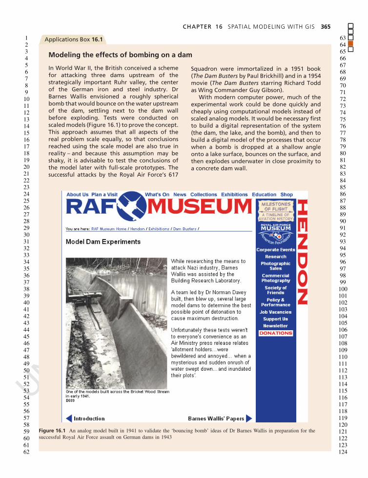
In World War II, the British conceived a schemefor attacking three dams upstream of thestrategically important Ruhr valley, the centerof the German iron and steel industry. DrBarnes Wallis envisioned a roughly sphericalbomb that would bounce on the water upstreamof the dam, settling next to the dam wallbefore exploding. Tests were conducted onscaled models (Figure 16.1) to prove the concept.This approach assumes that all aspects of thereal problem scale equally, so that conclusionsreached using the scale model are also true inreality – and because this assumption may beshaky, it is advisable to test the conclusions ofthe model later with full-scale prototypes. Thesuccessful attacks by the Royal Air Force’s 617

Squadron were immortalized in a 1951 book(The Dam Busters by Paul Brickhill) and in a 1954movie (The Dam Busters starring Richard Toddas Wing Commander Guy Gibson).

With modern computer power, much of theexperimental work could be done quickly andcheaply using computational models instead ofscaled analog models. It would be necessary firstto build a digital representation of the system(the dam, the lake, and the bomb), and then tobuild a digital model of the processes that occurwhen a bomb is dropped at a shallow angleonto a lake surface, bounces on the surface, andthen explodes underwater in close proximity toa concrete dam wall.

Figure 16.1 An analog model built in 1941 to validate the ‘bouncing bomb’ ideas of Dr Barnes Wallis in preparation for thesuccessful Royal Air Force assault on German dams in 1943

UNCORRECTED PROOFS

1234567891011121314151617181920212223242526272829303132333435363738394041424344454647484950515253545556575859606162

63646566676869707172737475767778798081828384858687888990919293949596979899

100101102103104105106107108109110111112113114115116117118119120121122123124


shortest distance over which change is recorded. Temporalresolution is also important, being defined as the shortesttime over which change is recorded and in the case ofmany dynamic models corresponding to the time intervalbetween iterations.

Spatial and temporal resolution are critical factors inmodels. They define what is left out of the model, inthe form of variation that occurs over distances or timesthat are less than the appropriate resolution. They alsotherefore define one major source of uncertainty in themodel’s outcomes. Uncertainty in this context can bedefined best through a comparison between the model’soutcomes and the outcomes of the real processes thatthe model seeks to emulate. Any model leaves its useruncertain to some degree about what the real world willdo – a measure of uncertainty attempts to give that degreeof uncertainty an explicit magnitude. Uncertainty has beendiscussed in the context of geographic data in Chapter 6;its meaning and treatment are discussed in the context ofspatial modeling later in this chapter.

Any model leaves its user uncertain to somedegree about what the real world will do.

Spatial and temporal resolution also determine thecost of acquiring the data because in general it is morecostly to collect a high-resolution representation than alow-resolution one. More observations have to be madeand more effort is consumed in making them. They alsodetermine the cost of running the model, since executiontime expands as more data have to be processed andmore iterations have to be made. One benchmark is ofcritical importance for many dynamic models: they mustrun faster than the processes they seek to simulate if theresults are to be useful for planning. One expects this to betrue of computational models, but in practice the amountof computing can be so large that the model simulationslows to unacceptable speed.

Spatial resolution is a major factor in the cost bothof acquiring data for modeling, and of actuallyrunning the model.

16.1.1 Why model?

Models are built for a number of reasons. First, a modelmight be built to support a design process, in which theuser wishes to find a solution to a spatial problem thatoptimizes some objective. This concept was discussed inSection 15.3 in the context of locating both point-likefacilities such as retail stores or fire stations, and line-like facilities such as transmission corridors or highways.Often the design process will involve multiple criteria, anissue discussed in Section 16.4.

Second, a model might be built to allow the userto experiment on a replica of the world, rather thanon the real thing. This is a particularly useful approachwhen the costs of experimenting with the real thingare prohibitive, or when unacceptable impacts would

result, or when results can be obtained much fasterwith a model. Medical students now routinely learnanatomy and the basics of surgery by working withdigital representations of the human body, rather thanwith expensive and hard-to-get cadavers. Humanity iscurrently conducting an unprecedented experiment on theglobal atmosphere by pumping vast amounts of CO2

into it. How much better it would have been if wecould have run the experiment on a digital replica, andunderstood the consequences of CO2 emissions well inadvance.

Experiments embody the notion of what-if scenarios,or policy alternatives that can be plugged into a model inorder to evaluate their outcomes. The ability to examinesuch options quickly and effectively is one of the majorreasons for modeling (Figure 16.2).

Models allow planners to experiment with‘what-if’ scenarios.

Finally, models allow the user to examine dynamicoutcomes, by viewing the modeled system as it evolvesand responds to inputs. As discussed in the next section,such dynamic visualizations are far more compelling andconvincing when shown to stakeholders and the publicthan descriptions of outcomes or statistical summaries.Scenarios evaluated with dynamic models are thus a veryeffective way of motivating and supporting debates overpolicies and decisions.

16.1.2 To analyze or to model?

Section 2.3.4.2 discussed the work of Tom Cova inanalyzing the difficulty of evacuating neighborhoodsin Santa Barbara, California, USA, in response to anemergency caused, for example, by a rapidly movingwildfire. The analysis provided useful results that couldbe employed by planners in developing traffic controlstrategies, or in persuading residents to use fewer carswhen they evacuate their homes. But the results arepresented in the form of static maps that must be explainedto residents, who might not otherwise understand the roleof the street pattern and population density in makingevacuation difficult.

By contrast, Box 16.2 describes the dynamic sim-ulations developed by Richard Church. These produceoutcomes in the form of dramatic animations that areinstantly meaningful to residents and planners. Theresearcher is able to examine what-if scenarios by varyinga range of parameters, including the number of vehiclesper household in the evacuation, the distribution of trafficcontrol personnel, the use of private and normally gatedexit roads, and many other factors. Simulations like thesecan galvanize a community into action far more effec-tively than static analysis.

Models can be used for dynamic simulation,providing decision makers with dramaticvisualizations of alternative futures.

UNCORRECTED PROOFS

123456789

1011121314151617181920212223242526272829303132333435363738394041424344454647484950515253545556575859606162

63646566676869707172737475767778798081828384858687888990919293949596979899100101102103104105106107108109110111112113114115116117118119120121122123124


Figure 16.2 A ‘live’ table constructed by Antonio Camara and his group (see Box 11.5) as a tool for examining alternativeplanning scenarios. The image on the table is projected from a computer and users are able to ‘move’ objects that represent sourcesof pollution around on the image by interacting directly with the display. Each new position results in the calculation of a hydrologicmodel of the impacts of the sources, and the display of the resulting pattern of impacts on the table

Biographical Box 16.2

Richard Church and traffic simulation

Figure 16.3 Richard Church,Professor of Geography, Universityof California, Santa Barbara

Richard Church (Figure 16.3) received his Bachelor of Science degree fromLewis and Clark College. After finishing two majors, one in Math andone in Chemistry, he continued his graduate education in Geographyand Environmental Engineering at The Johns Hopkins University wherehe specialized in water resource systems engineering. Currently, Rick isProfessor of Geography at the University of California, Santa Barbara. Hecontinues to be involved in environmental modeling and has specialized inforest systems modeling and ecological reserve design. He also teaches andconducts research in the area of logistics, transportation, urban planningand location modeling.

Rick is often motivated by real-world problems, whether it is operatinga reservoir, designing an ambulance posting plan for a city, or finding thebest corridor for a right-of-way.

One of his recent projects involves simulating the emergency evacuationof a neighborhood in advance of a rapidly moving fire, such as the one inthe Oakland Hills in 1991 that destroyed 2900 structures and resulted in 25deaths. Figure 16.4 shows the Mission Canyon area of Santa Barbara, a neighborhood that exhibits many ofthe same characteristics as the Oakland Hills.

Aware of the potential threat, members of the Mission Canyon neighborhood association asked if therewas a way in which then could better understand the difficulty then would face in an evacuation? To address

UNCORRECTED PROOFS

1234567891011121314151617181920212223242526272829303132333435363738394041424344454647484950515253545556575859606162

63646566676869707172737475767778798081828384858687888990919293949596979899

100101102103104105106107108109110111112113114115116117118119120121122123124


this problem Church utilized a micro-scale traffic simulation program called PARAMICS to model a numberof evacuation scenarios. Figure 16.5 shows the simulated pattern some minutes into an evacuation, with carsbumper-to-bumper crowding the available exits, and unable to move should the fire advance over them.Through this work, it was evident that the biggest gain in safety was to encourage residents to use onevehicle per household in making a quick exit. Furthermore, traffic control was found to be very important

Figure 16.4 The Mission Canyon neighborhood in Santa Barbara, California, USA (highlighted in red), a critical area forevacuation in a wildfire emergency. Note the contorted network of streets in this topographically rugged area

Figure 16.5 Simulation of driver behavior in a Mission Canyon evacuation some minutes after the initial evacuation order. The reddots denote the individual vehicles whose behavior is modeled in this simulation

UNCORRECTED PROOFS

123456789

1011121314151617181920212223242526272829303132333435363738394041424344454647484950515253545556575859606162

63646566676869707172737475767778798081828384858687888990919293949596979899100101102103104105106107108109110111112113114115116117118119120121122123124


in decreasing overall clearing time. The County Government has since agreed to pre-position traffic controlofficers during ‘red flag’ alerts (times of extreme fire danger) so that the time to respond with traffic controlmeasures is kept as low as possible. The work reported here was sponsored by a grant from the CaliforniaDepartment of Transportation (Caltrans).

The simulations using PARAMICS raise an important issue for GIS. The conventional representation of astreet in a GIS is as a polyline, a series of points connected by straight lines. However it would be impossibleto simulate driver behavior on such a representation because it would be necessary to slow to negotiate thesharp bends at each vertex. Instead PARAMICS uses a representation consisting of a series of circular arcs withno change of direction where arcs join. Integrating PARAMICS with GIS therefore requires transformationsoftware to convert polylines to acceptable representations (Figure 16.6).

Figure 16.6 The representation problem for driver simulation. The green line shows a typical polyline representation found in aGIS. But a simulated driver would have to slow almost to a halt to negotiate the sharp corners. Traffic simulation packages such asPARAMICS require a representation of circular arcs (the black line) with no change of direction where the arcs join (at the pointsindicated by red lines)

In summary, analysis as described in Chapters 14and 15 is characterized by:

■ A static approach, at one point in time;

■ The search for patterns or anomalies, leading to newideas and hypotheses; and

■ Manipulation of data to reveal what would otherwisebe invisible.

By contrast, modeling is characterized by:

■ Multiple stages, perhaps representing different pointsin time;

■ Implementing ideas and hypotheses; and

■ Experimenting with policy options and scenarios.

16.2 Types of model

16.2.1 Static models and indicators

A static model represents a single point in time andtypically combines multiple inputs into a single output.

There are no time steps and no loops in a static model,but the results are often of great value as predictors orindicators. For example, the Universal Soil Loss Equation(USLE, first discussed in Section 1.3) falls into thiscategory. It predicts soil loss at a point, based on fiveinput variables, by evaluating the equation:

A = R × K × LS × C × P

where A denotes the predicted erosion rate, R is theRainfall and Runoff Factor, K is the Soil ErodibilityFactor, LS is the Slope Length Gradient Factor, C isthe Crop/Vegetation and Management Factor, and P isthe Support Practice Factor. Full definitions of each ofthese variables and their measurement or estimation canbe found in descriptions of the USLE (see for examplehttp://www.co.dane.wi.us/landconservation/uslepg.htm).

A static model represents a system at a singlepoint in time.

The USLE passes the first test of a spatial modelin that many if not all of its inputs will vary spatiallywhen applied to a given area. But it does not passthe second test, since moving the points at which A isevaluated will not affect the results. Why, then, use aGIS to evaluate the USLE? There are three good reasons:

UNCORRECTED PROOFS

1234567891011121314151617181920212223242526272829303132333435363738394041424344454647484950515253545556575859606162

63646566676869707172737475767778798081828384858687888990919293949596979899

100101102103104105106107108109110111112113114115116117118119120121122123124


1) because some of the inputs, particularly LS, requirea GIS for their calculation from readily available data,such as digital elevation models; 2) because the inputsand output are best expressed, visualized, and used inmap form, rather than as tables of point observations; and3) because the inputs and outputs of the USLE are oftenintegrated with other types of data, for further analysisthat may require a GIS. Nevertheless, it is possible toevaluate the USLE in a simple spreadsheet applicationsuch as Excel, and the website cited in the previousparagraph includes a downloadable Excel macro for thispurpose.

Models that combine a variety of inputs to producean output are widely used, particularly in environmentalmodeling. The DRASTIC model calculates an index ofgroundwater vulnerability from input layers by apply-ing appropriate weights to the inputs (Figure 16.7).Box 16.3 describes another application, the calculationof a groundwater protection model, from several inputsin a karst environment (an area underlain by potentiallysoluble limestone, and therefore having substantial andrapid groundwater flow through cave passages). It usesESRI’s ModelBuilder software which is described laterin Section 16.3.1.

Figure 16.7 The results of using the DRASTIC groundwater vulnerability model in an area of Ohio, USA. The model combinesGIS layers representing factors important in determining groundwater vulnerability, and displays the results as a map ofvulnerability ratings

UNCORRECTED PROOFS

123456789

1011121314151617181920212223242526272829303132333435363738394041424344454647484950515253545556575859606162

63646566676869707172737475767778798081828384858687888990919293949596979899100101102103104105106107108109110111112113114115116117118119120121122123124


16.2.2 Individual and aggregatemodels

The simulation model described in Box 16.2 works at theindividual level, by attempting to forecast the behavior ofeach driver and vehicle in the study area. By contrast,it would clearly be impossible to model the behavior

of every molecule in the Mammoth Cave watershed,and instead any modeling of groundwater movementmust be done at an aggregate level, by predicting themovement of water as a continuous fluid. In general,models of physical systems are forced to adopt aggregateapproaches because of the enormous number of individualobjects involved, whereas it is much more feasible tomodel individuals in human systems, or in studies of

Applications Box 16.3

Building a groundwater protection model in a Karst environment

Rhonda Pfaff (ESRI staff) and Alan Glennon(a doctoral candidate at the University ofCalifornia, Santa Barbara) describe a simplebut elegant application of modeling to thedetermination of groundwater vulnerabilityin Kentucky’s Mammoth Cave watershed.Mammoth Cave is protected as a National Park,containing extensive and unique environments,but is subject to potentially damaging runofffrom areas in the watershed outside parkboundaries and therefore not subject tothe same levels of environmental protection.Figure 16.8 shows a graphic rendering of themodel in ESRI’s ModelBuilder. Each operationis shown as a rectangle and each dataset asan ellipse. Reading from top left, the modelfirst clips the slope layer to the watershed, thenselects slopes greater than or equal to 5 degrees.

A landuse layer is analyzed to select fields usedfor growing crops, and these are then combinedwith the steep slopes layer to identify crop fieldson steep slopes. A dataset of streams is bufferedto 300 m, and finally this is combined to forma layer identifying all areas that are crop fields,on steep slopes, within 300 m of a stream. Suchareas are particularly likely to experience soilerosion and to generate runoff contaminatedwith agricultural chemicals, which will thenimpact the downstream cave environment withits endangered populations of sightless fish.Figure 16.9 shows the resulting map.

A detailed description of this application isavailable at http://www.esri.com/news/arcuser/0704/files/modelbuilder.pdf, and the datasets areavailable at http://www.esri.com/news/arcuser/0704/summer2004.html.

Figure 16.8 Graphic representation of the groundwater protection model developed by Rhonda Pfaff and Alan Glennon for analysisof groundwater vulnerability in the Mammoth Cave watershed, Kentucky, USA

�

UNCORRECTED PROOFS

1234567891011121314151617181920212223242526272829303132333435363738394041424344454647484950515253545556575859606162

63646566676869707172737475767778798081828384858687888990919293949596979899

100101102103104105106107108109110111112113114115116117118119120121122123124


�

Figure 16.9 Results of the groundwater protection model. Highlighted areas are farmed for crops, on relatively steep slopes andwithin 300 m of streams. Such areas are particularly likely to generate runoff contaminated by agricultural chemicals and soil erosionand to impact adversely the cave environment into which the area drains

animal behavior. Even when modeling the movementof water as a continuous fluid it is still necessary tobreak the continuum into discrete pieces, as it is inthe representation of continuous fields (see Figure 3.11).Some models adopt a raster approach and are commonlycalled cellular models (see Section 16.2.3). Other modelsbreak the world into irregular pieces or polygons, as inthe case of the groundwater protection model describedin Box 16.3.

Aggregate models are used when it is impossibleto model the behavior of every individual elementin a system.

Models of individuals are often termed agent-basedmodels (ABM) or autonomous agent models (Box 16.4).With the massive computing power now available onthe desktop, and with techniques of object-orientedprogramming, it is comparatively easy to build andexecute ABMs, even when the number of agents is itselfmassive. Such models have been used to analyze andsimulate many types of animal behavior, as well as thebehavior of pedestrians in streets (Box 16.4), shoppersin stores, and drivers on congested roads (Box 16.2).They have also been used to model the behavior of

decision makers, not through their movements in spacebut through the decisions they make regarding spatialfeatures. For example, ABMs have been constructed tomodel the decisions made over land use in rural areas,by formulating the rules that govern individual decisionsby landowners in response to varying market conditions,policies, and regulations. The impact of these factors onthe fragmentation of the landscape, with its implicationsfor wildlife habitat, are of key interest in such models.

16.2.3 Cellular models

Cellular models, which were introduced in Section 2.3.5.1,represent the surface of the Earth as a raster. Each cell in thefixed raster has a number of possible states, which changethrough time as a result of the application of transitionrules. Typically the rules are defined over each cell’sneighborhood, and determine the outcome of each stagein the simulation based on the cell’s state, the states ofits neighbors, and the values of cell attributes. The studyof cellular models was first popularized by the work ofJohn Conway, Professor of Mathematics at Princeton, whostudied the properties of a model he called the Game ofLife (Box 16.5).

UNCORRECTED PROOFS

123456789

1011121314151617181920212223242526272829303132333435363738394041424344454647484950515253545556575859606162

63646566676869707172737475767778798081828384858687888990919293949596979899100101102103104105106107108109110111112113114115116117118119120121122123124


Technical Box 16.4

Agent-based models of movement in crowded spaces

Working at the University College London Cen-tre for Advanced Spatial Analysis, geographerand planner Michael Batty uses GIS to sim-ulate the disasters and emergencies that canoccur when large-scale events generate conges-tion and panic in crowds (Figure 16.10). Theevents involve large concentrations of peoplein small spaces that can arise because of acci-dents, terrorist attacks, or simply by the buildup of congestion through the convergence oflarge numbers of people into spaces with toolittle capacity. He has investigated scenarios fora number of major events, such as the move-ment of very large numbers of people to Meccato celebrate the Hajj (a holy event in the Mus-lim calendar; Figure 16.10) and the Notting HillCarnival (Europe’s largest street festival, heldannually in West Central London). His workuses agent-based models that take GIScienceto a finer level of granularity and incorporatetemporal processes as well as spatial structure.Fundamental to agent-based modeling of suchsituations is the need to understand how indi-viduals in crowds interact with each other andwith the geometry of the local environment.

Batty and his colleagues have been concernedwith modeling the behavior of individual humanagents under a range of crowding scenarios. Thisstyle of model is called agent-based because it

depends on simulating the aggregate effect ofthe behaviors of individual objects or persons inan inductive way (bottom-up: Section 4.9). Themodeling is based on averages – our objectiveis modeling an aggregate outcome (such as theonset of panic) although the particular behaviorof each agent is a combination of responseswhich are based on how routine behavior ismodified by the presence of other agents andby the particular environment in which theagent finds himself or herself. It is possibleto simulate a diverse range of outcomes, eachbased on different styles of interaction betweenindividual agents and different geometricalconfigurations of constraints.

Figure 16.11 shows one of Batty’s simula-tions of the interactions between two crowds.Here, a parade is moving around a street inter-section – the central portion of the movement(walkers in white) is the parade and the walkersaround this in gray/red are the watchers. Thismodel can be used to simulate the build-up ofpressure through random motion which thengenerates a breakthrough of the watchers intothe parade, an event that often leads to disas-ters of the kind experienced in festivals, rockconcerts, and football matches as well as ritualsituations like the Hajj.

Figure 16.10 Massive crowds congregate in Mecca during the annual Hajj. On February 1, 2004 244 pilgrims were trampled whenpanic stampeded the crowd. This was a unique but unfortunately not a freak occurrence: 50 pilgrims were killed in 2002, 35 in 2001,107 in 1998, and 1425 were killed in a pedestrian tunnel in 1990

�

UNCORRECTED PROOFS

1234567891011121314151617181920212223242526272829303132333435363738394041424344454647484950515253545556575859606162

63646566676869707172737475767778798081828384858687888990919293949596979899

100101102103104105106107108109110111112113114115116117118119120121122123124


�(A) (B)

Figure 16.11 Simulation of the movement of individuals during a parade. Parade walkers are in white, watchers in red. Thewatchers (A) build up pressure on restraining barriers and crowd control personnel, and (B) break through into the parade

Cellular models represent the surface of the Earthas a raster, each cell having a number of statesthat are changed at each iteration by theexecution of rules.

Several interesting applications of cellular methodshave been identified, and particularly outstanding are theefforts to apply them to urban growth simulation. Thelikelihood of a parcel of land developing depends onmany factors, including its slope, access to transportationroutes, status in zoning or conservation plans, but aboveall its proximity to other development. These models

express this last factor as a simple modification of therules of the Game of Life – the more developed thestate of neighboring cells, the more likely a cell isto make the transition from undeveloped to developed.Figure 16.13 shows an illustration from one such model,that developed by Keith Clarke and his co-workers atthe University of California, Santa Barbara, to predictgrowth patterns in the Santa Barbara area through 2040.The model iterates on an annual basis, and the effectsof neighboring states in promoting infilling are clearlyevident. The inputs for the model – the transportationnetwork, the topography, and other factors – are readily

Technical Box 16.5

The Game of Life

The game is played on a raster. Each cell has twostates, live and dead, and there are no additionalcell attributes (no variables to differentiate thespace), as there would be in GIS applications.Each cell has eight neighbors (the Queen’s case,Figure 15.19). There are three transition rules ateach time-step in the game:

1. A dead cell with exactly three live neighborsbecomes a live cell;

2. A live cell with two or three live neighborsstays alive; and

3. In all other cases a cell dies or remains dead.

With these simple rules it is possibleto produce an amazing array of patternsand movements, and some surprisingly sim-ple and elegant patterns emerge out of thechaos (in the field of agent-based model-ing these unexpected and simple patterns areknown as emergent properties). The pagehttp://www.math.com/students/wonders/life/life.html includes extensive details on the game,examples of particularly interesting patterns,and executable Java code. Figure 16.12 showsthree stages in an execution of the Game of Life.

UNCORRECTED PROOFS

123456789

1011121314151617181920212223242526272829303132333435363738394041424344454647484950515253545556575859606162

63646566676869707172737475767778798081828384858687888990919293949596979899100101102103104105106107108109110111112113114115116117118119120121122123124


(A) (B)

(C)

Figure 16.12 Three stages in an execution of the Game of Life: (A) the starting configuration, (B) the pattern after one time-step,and (C) the pattern after 14 time-steps. At this point all features in the pattern remain stable

Figure 16.13 Simulation of future urban growth patterns in Santa Barbara, California, USA. (Upper) growth limited by currenturban growth boundary; (Lower) growth limited only by existing parks (Courtesy: Keith Clarke)

UNCORRECTED PROOFS

1234567891011121314151617181920212223242526272829303132333435363738394041424344454647484950515253545556575859606162

63646566676869707172737475767778798081828384858687888990919293949596979899

100101102103104105106107108109110111112113114115116117118119120121122123124


prepared in GIS, and the GIS is used to output the resultsof the simulation.

One of the most important issues in such modeling iscalibration and validation – how do we know the rules areright, and how do we confirm the accuracy of the results?Clarke’s group has calibrated the model by brute force, byrunning the model forwards from some point in the pastunder different sets of rules and comparing the results tothe actual development history from then to the present.This method is extremely time-consuming since the modelhas to be run under vast numbers of combinations ofrules, but it provides at least some degree of confidencein the results. The issue of accuracy is addressed in moredetail, and with reference to modeling in general, later inthis chapter.

A model must be calibrated against real data todetermine appropriate values for its parametersand to ensure that its rules are valid.

16.2.4 Cartographic modeling andmap algebra

In essence, modeling consists of combining many stagesof transformation and manipulation into a single whole,for a single purpose. In the example in Box 16.3 thenumber of stages was quite small – only six – whereas inthe Clarke urban growth model several stages are executedmany times as the model iterates through its annual steps.

The individual stages can consist of a vast number ofoptions, encompassing all of the basic transformations ofwhich GIS is capable. In Section 14.1.2 it was argued thatGIS manipulations could be organized into six categories,depending on the broad conceptual objectives of eachmanipulation. But the six are certainly not the onlyway of classifying and organizing the numerous methodsof spatial analysis into a simple scheme. Perhaps themost successful is the one developed by Dana Tomlinand known as cartographic modeling or map algebra. Itclassifies all GIS transformations of rasters into four basicclasses, and is used in several raster-centric GISs as thebasis for their analysis languages:

■ local operations examine rasters cell by cell,comparing the value in each cell in one layer with thevalues in the same cell in other layers;

■ focal operations compare the value in each cell withthe values in its neighboring cells – most ofteneight neighbors;

■ global operations produce results that are true of theentire layer, such as its mean value;

■ zonal operations compute results for blocks ofcontiguous cells that share the same value, such as thecalculation of shape for contiguous areas of the sameland use, and attach their results to all of the cells ineach contiguous block.

With this simple schema, it is possible to express anymodel, such as Clarke’s urban growth simulation, as a

script in a well-defined language. The only constraint isthat the model inputs and outputs be in raster form.

Map algebra provides a simple language in whichto express a model as a script.

A more elaborate map algebra has been devised andimplemented in the PCRaster package, developed forspatial modeling at the University of Utrecht (pcras-ter.geog.uu.nl). In this language, a symbol refers to anentire map layer, so the command A = B + C takes thevalues in each cell of layers B and C, adds them, andstores the result as layer A.

16.3 Technology for modeling

16.3.1 Operationalizing models in GIS

Many of the ideas needed to implement models at apractical level have already been introduced. In thissection they are organized more coherently in a reviewof the technical basis for modeling.

Models can be defined as sequences of operations,and we have already seen how such sequences can beexpressed either as graphic flowcharts or as scripts. Oneof the oldest graphic platforms for modeling is Stella,now very widely distributed and popular as a means ofconceptualizing and implementing models. Although itnow has good links to GIS, its approach is conceptuallynon-spatial, so it will not be described in detail here.Instead, the focus will be on similar environments thatare directly integrated with GIS. The first of these mayhave been ERDAS’s Imagine software (www.gis.leica-geosystems.com/Products/Imagine/), which allows theuser to build complex modeling sequences from primitiveoperations, with a focus on the manipulations needed inimage processing and remote sensing. ESRI introduceda graphic interface to modeling in ArcView 3.x SpatialModeler, and enhanced it in ArcGIS 9.0 ModelBuilder(see Figure 16.8).

Any model can be expressed as a script, or visuallyas a flowchart.

Typically in these interfaces, datasets are representedas ellipses, operations as rectangles, and the sequence ofthe model as arrows. The user is able to modify andcontrol the operation sequence by interacting directly withthe graphic display.

Fully equivalent, but less visual and therefore moredemanding on the user, are scripts, which express modelsas sequences of commands, allowing the user to executean entire sequence by simply invoking a script. Initialefforts to introduce scripting to GIS were cumbersome,requiring the user to learn a product-specific languagesuch as ESRI’s AML (Arc Macro Language) or Avenue.

UNCORRECTED PROOFS

123456789

1011121314151617181920212223242526272829303132333435363738394041424344454647484950515253545556575859606162

63646566676869707172737475767778798081828384858687888990919293949596979899100101102103104105106107108109110111112113114115116117118119120121122123124


Today, it is common for GIS model scripts to be writtenin such industry-standard languages as Visual Basic forApplications (VBA), Perl, JScript, or Python. Scriptscan be used to execute GIS operations, request inputfrom the user, display results, or invoke other software.With interoperability standards such as Microsoft’s COM(Box 7.3), it is possible to call operations from anycompliant package from the same script. For example, ascript might combine GIS operations with calls to Excelfor simple tabular functions, or even calls to anothercompliant GIS (Section 7.6).

With standards like Microsoft’s COM it is possiblefor a script to call operations from several distinctsoftware packages.

16.3.2 Model coupling

The previous section described the implementation ofmodels as direct extensions of an underlying GIS, througheither graphic model-building or scripts. This approachmakes two assumptions: first, that all of the operationsneeded by the model are available in the GIS (or inanother package that can be called by the model); andsecond, that the GIS provides sufficient performance tohandle the execution of the model. In practice, a GISwill often fail to provide adequate performance, especiallywith very large datasets and large numbers of iterations,because it has not been designed as a modeling engine.Instead, the user is forced to resort to specialized code,written in a source language such as C. Clarke’s model,for example, is programmed in C, and the GIS is used onlyfor preparing input and visualizing output. Other modelsmay be spatial only in the sense of having geographicallydifferentiated inputs and outputs, as discussed in the caseof the USLE in Section 16.2.1, making the use of a GISoptional rather than essential.

In reality, therefore, much spatial modeling is done bycoupling GIS with other software. A model is said to beloosely coupled to a GIS when it is run as a separatepiece of software and data are exchanged to and fromthe GIS in the form of files. Since many GIS formatsare proprietary, it is common for the exchange files tobe in export format, and to rely on translators at eitherend of the transfer. In extreme cases it may be necessaryto write a special program to convert the files duringtransfer, when no common format is available. Clarke’s isan example of a model that is loosely coupled to GIS. Amodel is said to be closely coupled to a GIS when both themodel and the GIS read and write the same files, obviatingany need for translation. When the model is executed asa GIS script or through a graphic GIS interface it is saidto be embedded.

16.3.3 Cataloging and sharing models

In the digital computer everything – the program, thedata, the metadata – must be expressed in the samelanguage of 0s and 1s. The value of each bit or byte

(Box 3.1) depends on its meaning, and clearly somebits are more valuable than others. A bit in Microsoft’soperating system Windows XP is clearly extremelyvaluable, even though there are hundreds of millions ofthem. On the other hand, a bit in a remote sensing imagethat happens to have been taken on a cloudy day hasalmost no value at all, except perhaps to someone studyingclouds. In general, one would expect bits of programs tobe more valuable than bits of data, especially when thoseprograms are useable by large numbers of people.

This line of argument suggests that the GIS scripts,models, and other representations of process are poten-tially valuable to many users and well worth sharing. Butalmost all of the investment society has made in the shar-ing of digital information has been devoted to data andtext. In Section 11.2 we saw how geolibraries, data ware-houses, and metadata standards have been devised andimplemented to facilitate the sharing of geographic data,and parallel efforts by libraries, publishers, and buildersof search engines have made it easy nowadays to sharetext via the Web. But very little effort to date has goneinto making it possible to share process objects, digitalrepresentations of the process of GIS use.

A process object, such as a script, captures theprocess of GIS use in digital form.

Notable exceptions include ESRI’s ArcScripts, alibrary of GIS scripts contributed by users and maintainedby the vendor as a service to its customers. The libraryis easily searched for scripts to perform specific types ofanalysis and modeling. At the time of writing, it included3286 scripts, ranging from one to couple ArcView 3.xto the StormWater Management Model (SWMM) writtenin Avenue, to a set of basic tools for crime analysis andmapping. ArcGIS 9.0 includes the ability to save, catalog,and share scripts as GIS functions.

The term GIService is often used to describe a GISfunction being offered by a server for use by any userconnected to the Internet (see Sections 1.5.3 and 7.2). Inessence, GIServices offer an alternative to locally installedGIS, allowing the user to send a request to a remote siteinstead of to his or her GIS. GIServices are particularlyeffective in the following circumstances:

■ When it would be too complex, costly, ortime-consuming to install and run the service locally;

■ When the service relies on up-to-date data that wouldbe too difficult or costly for the user toconstantly update;

■ When the person offering the service wishes tomaintain control over his or her intellectual property.This would be important, for example, when thefunction is based on a substantial amount ofknowledge and expertise.

To date, several standard GIS functions are availableas GIServices, satisfying one or more of the aboverequirements. The Alexandria Digital Library offers agazetteer service (www.alexandria.ucsb.edu), allowinga user to send a placename and to receive in returnone or more coordinates of places that match the pla-cename. Several companies offer geocoding services,

UNCORRECTED PROOFS

1234567891011121314151617181920212223242526272829303132333435363738394041424344454647484950515253545556575859606162

63646566676869707172737475767778798081828384858687888990919293949596979899

100101102103104105106107108109110111112113114115116117118119120121122123124


returning coordinates in response to a street address(try www.geocode.com). The Geography Network(www.geographynetwork.com) provides a searchablecatalog to GIServices.

16.4 Multicriteria methods

The model developed by Pfaff and Glennon (depicted inFigure 16.8) rates vulnerability to runoff based on threefactors – cropland, slope, and distance from stream – buttreats all three as simple binary measures, and produces asimple binary result (land is vulnerable if slope is greaterthan 5%, land use is cropping, and distance from streamis less than 300 m). In reality, of course, 5% is nota precise cutoff between non-vulnerable and vulnerableslopes, and neither is 300 m a precise cutoff betweenvulnerable distances and non-vulnerable distances. Theissues surrounding rules such as these, and their fuzzyalternatives, were discussed at length in Section 6.2.

A more general and powerful conceptual frameworkfor models like this would be constructed as follows.There are a number of factors that influence vulnerability,denoted by x1 through xn. The impact of each factoron vulnerability is determined by a transformation of thefactor f (x) – for example, the factor distance would betransformed so that its impact decreases with increasingdistance (as in Section 4.5), whereas the impact of slopewould be increasing. Then the combined impact of allof the factors is obtained by weighting and adding them,each factor i having a weight wi :

I =n∑

i=1

wif (xi)

In this framework both the functions f and the weightsw need to be determined. In the example, the f for slopewas resolved by a simple step function, but it seemsmore likely that the function should be continuouslydecreasing, as shown in Figure 16.14. The U-shapedfunction also shown in the figure would be appropriatein cases where the impact of a factor declines in bothdirections from some peak value (for example, smokefrom a tall smokestack has its greatest impact at somedistance downwind).

Many decisions depend on identifying relevantfactors and adding their appropriatelyweighted values.

This approach provides a good conceptual frameworkboth for the indicator models typified by Box 16.3 andfor many models of design processes. In both cases,it is possible that multiple views might exist aboutappropriate functions and weights, particularly whenmodeling a decision over an important development withimpact on the environment. Different stakeholders in thedesign process can be anticipated to have different views

magnitude x

impact f (x)

Figure 16.14 Three possible impact functions: (red) the stepfunction used to assess slope in Figure 16.8; (blue) adecreasing linear function; and (black) a function showingimpact rising to a maximum and then decreasing

about what is important, how that importance shouldbe measured, and how the various important factorsshould be combined. Such processes are termed multi-criteria decision making or MCDM, and are commonlyencountered whenever decisions are controversial. Somestakeholders may feel that environmental factors deservehigh weight, others that cost factors are the mostimportant, and still others that impact on the social life ofcommunities is all-important.

An important maxim of MCDM is that it is betterfor stakeholders to argue in principle about the meritsof different factors and how their impacts should bemeasured, than to argue in practice about alternativedecisions. For example, arguing about whether slope isa more important factor than distance, and about howeach should be measured, is better than arguing aboutthe relative merits of Solution A, which might color halfof John Smith’s field red, over Solution B, which mightcolor all of David Taylor’s field red. Ideally, all of thecontroversy should be over once the factors, functions,and weights are decided, and the solution they produceshould be acceptable to all, since all accepted the inputs.Would it were so!

Each stakeholder in a decision may have his or herown assessment of the importance of eachrelevant factor.

Although many GIS have implemented various appro-aches to MCDM, Clark University’s Idrisi offers themost extensive functionality as well as detailed tutorialsand examples (www.clarklabs.org; see Box 16.6). Acommon framework is the Analytical Hierarchy Process(AHP) devised by Thomas Saaty, which focuses oncapturing each stakeholder’s view of the appropriateweights to give to each impact factor. First, the impactof each factor is expressed as a function, choosing fromoptions such as those shown in Figure 16.14. Then eachstakeholder is asked to compare each pair of factors(with n factors there are n(n − 1)/2 pairs), and to assesstheir relative importance in ratio form. A matrix is

UNCORRECTED PROOFS

123456789

1011121314151617181920212223242526272829303132333435363738394041424344454647484950515253545556575859606162

63646566676869707172737475767778798081828384858687888990919293949596979899100101102103104105106107108109110111112113114115116117118119120121122123124


Table 16.1 An example of the weights assigned to threefactors by one stakeholder. For example, the entry ‘7’ in Row 1Column 2 (and the 1/7 in Row 2 Column 1) indicates that thestakeholder felt that Factor 1 (slope) is seven times asimportant as Factor 2 (land use)

Slope Land use Distance fromstream

Slope 7 2Land use 1/7 1/3Distance from stream 1/2 3

created for each stakeholder, as in the example shown inTable 16.1. The matrices are then combined and analyzed,and a single set of weights extracted that represent aconsensus view (Figure 16.15). These weights would thenbe inserted as parameters in the spatial model to producea final result. The mathematical details of the method canbe found in books or tutorials on the AHP.

16.5 Accuracy and validity: testingthe model

Models are complex structures and their outputs are oftenforecasts of the future. How, then, can a model be tested,and how does one know whether its results can be trusted?Unfortunately, there is an inherent tendency to trustthe results of computer models because they appear innumerical form (and numbers carry innate authority) andbecause they come from computers (which also appearauthoritative).

Results from computers tend to carryinnate authority.

Normally, scientists test their results against reality,but in the case of forecasts reality is not yet available,and by the time it is there is likely little interest in testing.So modelers must resort to other methods to verify andvalidate their predictions.

Figure 16.15 Screen shot of an AHP application using Idrisi (www.clarklabs.org). The five layers in the upper left part of thescreen represent five factors important to the decision. In the lower left, the image shows the table of relative weights compiled byone stakeholder. All of the weights matrices are combined and analyzed to obtain the consensus weights shown in the lower right,together with measures to evaluate consistency among the stakeholders (Courtesy: Clark Labs)

UNCORRECTED PROOFS

1234567891011121314151617181920212223242526272829303132333435363738394041424344454647484950515253545556575859606162

63646566676869707172737475767778798081828384858687888990919293949596979899

100101102103104105106107108109110111112113114115116117118119120121122123124


Biographical Box 16.6

Ron Eastman, developer of the Idrisi GIS

Figure 16.16 Ron Eastman,developer of Idrisi

J. Ronald Eastman (Figure 16.16) is Director and lead software engineerof Clark Labs, a non-profit center within the George Perkins MarshInstitute of Clark University that produces the Idrisi GIS and imageprocessing system, non-profit software with over 35 000 registered usersworldwide. He is also Professor of Geography and former Director of theGraduate School of Geography at Clark University. He gained his Ph.D. inGeography from Boston University in 1982. His research is focused moststrongly on the development of analytical procedures for the investigationand modeling of land-cover change and effective resource allocation inenvironmentally related decision making. He also has extensive experiencein the deployment of GIS and remote sensing in the developing world, and is a Senior Special Fellow of theUnited Nations Institute for Training and Research. He writes:

With a degree in perceptual psychology and a strong love of travel and the diversity of landscapes andcultures, I became interested in the power of the visual system in facilitating the analysis of geographicphenomena through the medium of maps. My graduate degrees were thus is geography/cartography.However, I had the fortune of witnessing and participating in the birth of GIS and digital image processing. Itwas immediately clear to me that the analytical potential of this new medium far outstripped what could beachieved by visual analysis alone, particularly in the study of our rapidly changing environment. At the sametime, I was also concerned that many in the developing world had only limited access to computing resourcesand GIS/image processing technology – thus my motivation in developing a system focused on the analyticalneeds of development and global change.

Models can often be tested by comparison with pasthistory, by running the model not into the future, butforwards in time from some previous point. But these areoften the data used to calibrate the model, to determineits parameters and rules, so the same data are notavailable for testing. Instead, many modelers resort tocross-validation, a process in which a subset of data isused for calibration, and the remainder for validatingresults. Cross-validation can be done by separating thedata into two time periods, or into two areas, using onefor calibration and one for validation. Both are potentiallydangerous if the process being modeled is also changingthrough time, or across space (it is non-stationary in astatistical sense), but forecasting is dangerous in thesecircumstances as well.

Models of real-world processes can be validated byexperiment, by proving that each component in the modelcorrectly reflects reality. For example, the Game of Lifewould be an accurate model if some real process actuallybehaved according to its rules; and Clarke’s urban growthmodel could be tested in the same way, by examiningthe rules that account for each past land use transition.In reality, it is unlikely that real-world processes willbe found to behave as simply as model rules, and it isalso unlikely that the model will capture every real-worldprocess impacting the system.

If models are no better than approximations to reality,then are they of any value? Certainly human society

is so complex that no model will ever fit perfectly.As Ernest Rutherford, the experimental physicist andNobel Laureate is said to have once remarked, probablyin frustration with social-scientist colleagues, ‘The onlyresult that can possibly be obtained in the social sciencesis, some do, and some don’t’. Neither will a model of aphysical system ever perfectly replicate reality. Instead,the outputs of models must always be taken advisedly,bearing in mind several important arguments:

■ A model may reflect behavior under idealcircumstances and therefore provide a norm againstwhich to compare reality. For example, manyeconomic models assume a perfectly informed,rational decision maker. Although humans rarelybehave this way, it is still useful to know what wouldhappen if they did, as a basis for comparison.

■ A model should not be measured by how closely itsresults match reality but by how much it reducesuncertainty about the future. If a model can narrowthe options, then it is useful. It follows that anyforecast should also be accompanied by a realisticmeasure of uncertainty.

■ A model is a mechanism for assembling knowledgefrom a range of sources and presenting conclusionsbased on that knowledge in readily used form. It isoften not so much a way of discovering how theworld works, as a way of presenting existingknowledge in a form helpful to decision-makers.

UNCORRECTED PROOFS

123456789

1011121314151617181920212223242526272829303132333435363738394041424344454647484950515253545556575859606162

63646566676869707172737475767778798081828384858687888990919293949596979899100101102103104105106107108109110111112113114115116117118119120121122123124


■ Just as the British politician Denis Healey onceremarked that capitalism was the worst possibleeconomic system ‘apart from all of the others’, somodeling often offers the only robust, transparentanalytical framework that is likely to garner anyrespect amongst decision makers with competingobjectives and interests.

Any model forecast should be accompanied by arealistic measure of uncertainty.

Several forms of uncertainty are associated withmodels, and it is important to distinguish between them.First, models are subject to the uncertainty present intheir inputs. Uncertainty propagation was discussed inSection 6.4.2 – here, it refers to the impacts of uncertaintyin the inputs of a model on uncertainty in the outputs.In some cases propagation may be such that an error oruncertainty in an input produces a proportionate error inan output. In other cases, a very small error in an inputmay produce a massive change in output; and in othercases outputs can be relatively insensitive to errors ininputs. It is important to know which of these cases holdsin a given instance, and the normal approach is throughrepeated numerical simulation (often called Monte Carlosimulation because it mimics the random processes of thatfamous gambling casino), adding random distortions toinputs and observing their impacts on outputs. In somelimited instances it may even be possible to determinethe effects of propagation mathematically.

Second, models are subject to uncertainty over theirparameters. A model builder will do the best possiblejob of calibrating the model, but inevitably there willbe uncertainty about the correct values, and no modelwill fit the data available for calibration perfectly. It isimportant, therefore, that model users conduct some formof sensitivity analysis, examining each parameter in turnto see how much influence it has on the results. This canbe done by raising and lowering each parameter value, forexample by +10% and −10%, re-running the model andcomparing the results. If changing a parameter by 10%produces a less-than-10% change in results the model canbe said to be relatively insensitive to that parameter. Thisallows the modeler to focus attention on those parametersthat produce the greatest impact on results, making everyeffort to ensure that their values are correct.

Sensitivity analysis tests a model’s response tochanges in its parameters and assumptions.

Third, and most importantly, models are subject touncertainty because of the labeling of their results. Con-sider the model of Box 16.3, which computes an indicatorof the need for groundwater protection. In truth, the areasidentified by the model have three characteristics – slopegreater than 5%, used for crops, and less than 300 m froma stream. Described this way, there is little uncertaintyabout the results, though there will be some uncertaintydue to inaccuracies in the data. But once the areas selectedare described as vulnerable, and in need of management toensure that groundwater is protected, a substantial leap oflogic has occurred. Whether that leap is valid or not willdepend on the reputation of the modeler as an expert ingroundwater hydrology and biological conservation; onthe reputation of the organization sponsoring the work;and on the background science that led to the choice ofparameters (5% and 300 m). In essence, this third type ofuncertainty, which arises whenever labels are attached toresults that may or may not correctly reflect their mean-ing, is related to how results are described, in other wordsto their metadata, rather than to any innate characteristicof the data themselves.

16.6 Conclusion

Modeling was defined at the outset of this chapter as aprocess involving multiple stages, often in emulation ofsome real physical process. Modeling is often dynamic,and current interest in modeling is stretching the capabil-ities of GIS software, most of which was designed for thecomparatively leisurely process of analysis, rather thanthe intensive and rapid iterations of a dynamic model. Inmany ways, then, modeling represents the cutting edgeof GIS, and the next few years are likely to see explo-sive growth both in interest in modeling on the part ofGIS users, and software development on the part of GISvendors. The results are certain to be interesting.

Questions for further study

1. Write down the set of rules that you would use toimplement a simple version of the Clarke urbangrowth model, using the following layers:transportation (cell contains road or not), protected(cell is not available for development), alreadydeveloped, and slope.

2. Review the steps you would take and the argumentsyou would use to justify the validity of aGIS-based model.

3. Select a field of environmental or social science, suchas species habitat prediction or residentialsegregation. Search the Web and your library forpublished models of processes in this field andsummarize their conceptual structure, technicalimplementation, and application history.

UNCORRECTED PROOFS

1234567891011121314151617181920212223242526272829303132333435363738394041424344454647484950515253545556575859606162

63646566676869707172737475767778798081828384858687888990919293949596979899

100101102103104105106107108109110111112113114115116117118119120121122123124

382 PART IV ANALYSIS382 PART IV ANALYSIS

4. Compare the relative advantages of the differenttypes of dynamic models discussed in this chapterwhen applied to a selected area of environmental orsocial science.

Further readingHeuvelink G.B.M. 1998 Error Propagation in Environ-

mental Modelling with GIS. London: Taylor andFrancis.

Saaty T.L. 1980 The Analytical Hierarchy Process: Plan-ning, Priority Setting, Resource Allocation. New York:McGraw-Hill.

Tomlin C.D. 1990 Geographic Information Systems andCartographic Modeling. Englewood Cliffs, NJ: Pren-tice Hall.

Spatial modeling with GIS - UC Santa Barbara

Documents

Transcript of Spatial modeling with GIS - UC Santa Barbara