Spatial Lag Regression
268
THE DYNAMIC INTERACTION BETWEEN RESIDENTIAL MORTGAGE FORECLOSURE, NEIGHBORHOOD CHARACTERISTICS, AND NEIGHBORHOOD CHANGE DISSERTATION Presented in Partial Fulfillment of the Requirements for the Degree Doctor of Philosophy in the Graduate School of The Ohio State University By Yanmei Li, M.A. ***** The Ohio State University 2006 Dissertation Committee: Professor Hazel Morrow-Jones, Adviser Professor Donald R. Haurin Professor Philip A. Viton Approved by Adviser Graduate Program in City and Regional Planning
Transcript of Spatial Lag Regression
8/6/2019 Spatial Lag Regression
http://slidepdf.com/reader/full/spatial-lag-regression 1/268
THE DYNAMIC INTERACTION BETWEEN RESIDENTIALMORTGAGE FORECLOSURE, NEIGHBORHOOD
CHARACTERISTICS, AND NEIGHBORHOOD CHANGE
DISSERTATION
Presented in Partial Fulfillment of the Requirements for
the Degree Doctor of Philosophy in the Graduate
School of The Ohio State University
By
Yanmei Li, M.A.
*****
The Ohio State University
2006
Dissertation Committee:
Professor Hazel Morrow-Jones, Adviser
Professor Donald R. Haurin
Professor Philip A. Viton
Approved by
AdviserGraduate Program in City and Regional
Planning

8/6/2019 Spatial Lag Regression
http://slidepdf.com/reader/full/spatial-lag-regression 2/268
Copyright by
Yanmei Li
2006
8/6/2019 Spatial Lag Regression
http://slidepdf.com/reader/full/spatial-lag-regression 3/268
ii
ABSTRACT
Many factors lead to mortgage default and foreclosure, and neighborhood
characteristics are among the most important (Quercia and Stegman, 1992). However,
few scholars have examined how neighborhood characteristics contribute to mortgage
foreclosure (Cotterman, 2001; Baxter and Lauria, 2000; Lauria, 1998) and none of the
previous studies have systematically addressed the mutual interaction between
foreclosure and neighborhood characteristics and change. This research uses multiple
datasets from Ohio’s two most populous counties to examine some of these previously
omitted or understudied aspects of the issue. Particular attention has been paid to each
neighborhood’s racial composition, economic level, housing prices and other housing
stock characteristics as well as to the changes over time in those variables.
The analysis starts with simple descriptive statistics, spatial autocorrelation analysis,
and comparison of different foreclosure patterns in the two counties. Then spatial
regression models, H-Robust models and Iterated Seemingly Unrelated Regression
(ITSUR) are used to explain the interaction between mortgage foreclosure and
neighborhood characteristics and change. The study finds that foreclosures cluster in low-
income minority neighborhoods and inner cities, although suburban areas have seen an
increase. Educational attainment, median household income, and average housing cost
burden contribute to foreclosures in both counties. As expected there are similarities and

8/6/2019 Spatial Lag Regression
http://slidepdf.com/reader/full/spatial-lag-regression 4/268
iii
disparities in the interaction of foreclosure and neighborhoods between the two counties.
The use of panel data, Robust OLS, spatial lag models and SUR has solved some
problems related to spatial dependence, heteroskedasticity and mutual non-recursive
interaction between foreclosure and neighborhoods.
The research not only contributes to the literate and methodology in related topics,
but also contributes to our understanding of the relationship between foreclosure and
neighborhoods, and will assist in the creation of better policies to deal with the issue of
foreclosure. The policy recommendations include a strong focus on neighborhood
foreclosure prevention, not just policies aimed at individual homeowners. These policies
might focus on neighborhoods with low educational attainment, an increasing percentage
black population, or a high female headship rate. This project suggests that foreclosure
prevention programs not be the same in all places.

8/6/2019 Spatial Lag Regression
http://slidepdf.com/reader/full/spatial-lag-regression 5/268
iv
Dedicated to my father and mother
8/6/2019 Spatial Lag Regression
http://slidepdf.com/reader/full/spatial-lag-regression 6/268
v
ACKNOWLEDGMENTS
I wish to thank my adviser, Professor Hazel Morrow-Jones, for her intellectual
support, encouragement, and enthusiasm that made this dissertation possible, and for her
patience in correcting my English, stylistic and scientific errors.
I thank Professor Jean M. Guldmann, Professor Phillip Viton, and Professor Donald
Haurin for their guidance which made the methodology more appealing.
I am grateful to Charlie Post from the Housing Research Center at Cleveland State
University to provide Cuyahoga County’s parcel data.
I wish to thank Katrin Anacker and Fang-Chi Hsu for their continuous
encouragement. I am indebted to Joe Gakenheimer for his support and suggestions in
writing and preparing this manuscript. I thank Eileen Frey, Cheryl Kaufman, and Donna
Fasnacht for their continuous prayers and love.
This research was supported by a grant from the Center for Urban and Regional
Analysis (CURA) at the Ohio State University. The financial support from the grant has
made this dissertation possible.
8/6/2019 Spatial Lag Regression
http://slidepdf.com/reader/full/spatial-lag-regression 7/268
vi
VITA
December 25, 1975 ..……..…………...Born - Qujing, China
1998 ……………………….…………..B.S. Geography, East China Normal University,Shanghai, China
2001 …………………………………M.A. Regional Economics, Beijing Normal
University, Beijing, China
2001 – present ………………………Graduate Research Associate, The Ohio StateUniversity
PUBLICATIONS
1. Wu, Dianting, Yanmei Li, et. al. 2002. The Development of Intellectual Economy inChina. Economic Geography (Chinese). Vol. 22, No. 4
2. Wu, Dianting, Jie Tian, Yanmei Li, et. al. 2002. The Analysis of the Relationships
between Modernization, Industrialization, Urbanization, Intellectualization andEconomic Development in China. Systems Engineering – Theory and Practice
(Chinese). Vol.22. No. 11.3. Li, Yanmei, Dianting Wu, and Gang Zeng, 1999. The Characteristics and
Development Strategies of Hi-tech in Changjiang Delta, Areal Research and
Development (Chinese), Vol.18, No.34. Wu, Dianting, Shen Ji, and Yanmei Li. 1998. Dividing One Integrated Part to Three
Sections in Geographic Thoughts, Youth Geographer(Chinese), Vol.9, No.4
FIELDS OF STUDY
Major Field: City and Regional Planning

8/6/2019 Spatial Lag Regression
http://slidepdf.com/reader/full/spatial-lag-regression 8/268
vii
TABLE OF CONTENTS
ABSTRACT ............................................................................................................. ii
ACKNOWLEDGMENTS................................................................................................ vVITA ................................................................................................................ vi
LIST OF TABLES........................................................................................................... ix
LIST OF FIGURES......................................................................................................... xi
CHAPTER 1 INTRODUCTION AND RESEARCH QUESTIONS......................... 1
Nature of the Problem..................................................................................................... 2Objective of the Research ............................................................................................... 3Research Questions......................................................................................................... 4Scope of the Research..................................................................................................... 6
CHAPTER 2 LITERATURE REVIEW...................................................................... 8Residential Mortgage Foreclosure .................................................................................. 8The Interaction between Neighborhood Characteristics, Neighborhood Change andResidential Mortgage Foreclosure ................................................................................ 31Major Problems in Neighborhood-Effects Research .................................................... 46Literature Summary and the Derivation of Research Questions .................................. 50
CHAPTER 3 RESEARCH METHODOLOGY........................................................ 52Hypotheses.................................................................................................................... 52Major Datasets Used in Foreclosure Research ............................................................. 56Summary of Datasets Used in this Research ................................................................ 62Variable Selection and Description .............................................................................. 64Research Methodology ................................................................................................. 73
CHAPTER 4 DESCRIPTIVE AND SPATIAL ANALYSIS .................................. 84Judicial Foreclosure Process and Sheriff’s Deed Transfer Data................................... 84Ohio’s Foreclosure Situation ........................................................................................ 87
Research Area and Geographic Definition of Neighborhood....................................... 91Data Description for Each County................................................................................ 99Conclusions................................................................................................................. 139
CHAPTER 5 THE INTERACTION BETWEEN RESIDENTIAL MORTGAGE
FORECLOSURE, NEIGHBORHOOD CHARACTERISTICS,
AND NEIGHBORHOOD CHANGE.............................................. 141Effects of Neighborhoods on Foreclosure .................................................................. 145

8/6/2019 Spatial Lag Regression
http://slidepdf.com/reader/full/spatial-lag-regression 9/268
viii
Summary: Effects of Neighborhood Characteristics on Residential MortgageForeclosure.................................................................................................................. 167The Impact of Residential Mortgage Foreclosure on Neighborhood Change: ASeemingly Unrelated Regression (SUR) Approach.................................................... 173Conclusion: The Interaction between Residential Mortgage Foreclosure, Neighborhood
Characteristics, and Neighborhood Change................................................................ 188
CHAPTER 6 CONCLUSIONS, POLICY IMPLICATIONS AND FUTURE
RESEARCH DIRECTIONS............................................................ 192
APPENDIX A FORECLOSURE PROCEDURES ................................................. 207
APPENDIX B TOTAL SHERIFF’S DEEDS AT THE SCHOOL DISTRICTLEVEL IN FRANKLIN COUNTY................................................. 214
APPENDIX C SPATIAL AUTOCORRELATION OF SELECTED VARIABLES
............................................................................................................. 216
APPENDIX D SUR MODEL RESULTS................................................................. 229
APPENDIX E THE GEOGRAPHIC DISTRIBUTION OF SELECTED
NEIGHBORHOOD CHANGE INDICATORS AT THE BLOCK
GROUP LEVEL IN FRANKLIN AND CUYAHOGA COUNTIES............................................................................................................. 233
BIBLIOGRAPHY…………………………………………………………….……….239
NOTES ……………………………………………………………………………….252
8/6/2019 Spatial Lag Regression
http://slidepdf.com/reader/full/spatial-lag-regression 10/268
ix
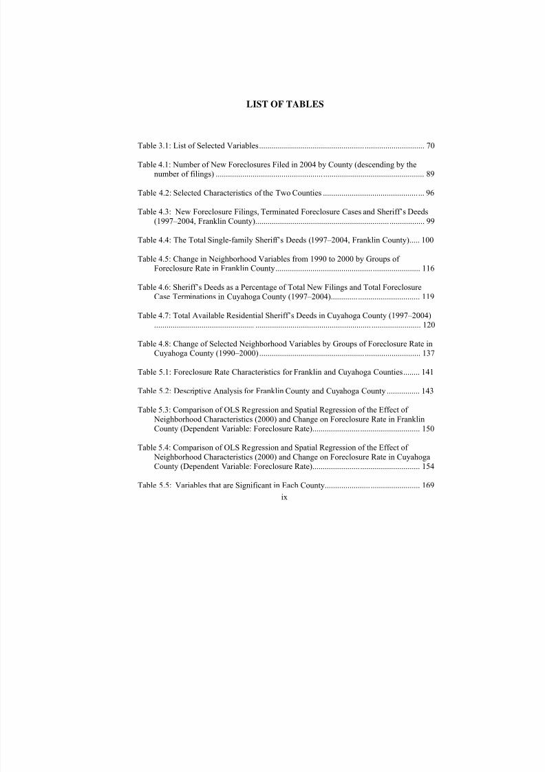
LIST OF TABLES
Table 3.1: List of Selected Variables................................................................................ 70
Table 4.1: Number of New Foreclosures Filed in 2004 by County (descending by thenumber of filings) ..................................................................................................... 89
Table 4.2: Selected Characteristics of the Two Counties ................................................. 96
Table 4.3: New Foreclosure Filings, Terminated Foreclosure Cases and Sheriff’s Deeds(1997–2004, Franklin County).................................................................................. 99
Table 4.4: The Total Single-family Sheriff’s Deeds (1997–2004, Franklin County)..... 100
Table 4.5: Change in Neighborhood Variables from 1990 to 2000 by Groups of Foreclosure Rate in Franklin County...................................................................... 116
Table 4.6: Sheriff’s Deeds as a Percentage of Total New Filings and Total ForeclosureCase Terminations in Cuyahoga County (1997–2004)........................................... 119
Table 4.7: Total Available Residential Sheriff’s Deeds in Cuyahoga County (1997–2004)................................................................................................................................. 120
Table 4.8: Change of Selected Neighborhood Variables by Groups of Foreclosure Rate inCuyahoga County (1990–2000) .............................................................................. 137
Table 5.1: Foreclosure Rate Characteristics for Franklin and Cuyahoga Counties........ 141
Table 5.2: Descriptive Analysis for Franklin County and Cuyahoga County ................ 143
Table 5.3: Comparison of OLS Regression and Spatial Regression of the Effect of
Neighborhood Characteristics (2000) and Change on Foreclosure Rate in FranklinCounty (Dependent Variable: Foreclosure Rate).................................................... 150
Table 5.4: Comparison of OLS Regression and Spatial Regression of the Effect of Neighborhood Characteristics (2000) and Change on Foreclosure Rate in CuyahogaCounty (Dependent Variable: Foreclosure Rate).................................................... 154
Table 5.5: Variables that are Significant in Each County.............................................. 169

8/6/2019 Spatial Lag Regression
http://slidepdf.com/reader/full/spatial-lag-regression 11/268
x
Table 5.6: Cross Model Covariance Matrix for Cuyahoga County ................................ 175
Table 5.7: ITSUR Estimate Results with “FORECLOSURE” (as an independent variable)Significant (System Weighted R-Square: 0.4104; System Weighted MSE: 1.0000)................................................................................................................................. 177
Table A.1: Legislation Requirement of Mortgage Foreclosure in Different States in theU.S. ......................................................................................................................... 208
Table B.1: Total Sheriff’s Deeds at the School District Level in Franklin County (1997-2004, Note: 11838 total cases and 6 cases can’t be identified at the school districtlevel) ....................................................................................................................... 215
Table D.1: ITSUR Estimate Results (where “FORECLOSURE” is not significant) ..... 230

8/6/2019 Spatial Lag Regression
http://slidepdf.com/reader/full/spatial-lag-regression 12/268
xi
LIST OF FIGURES
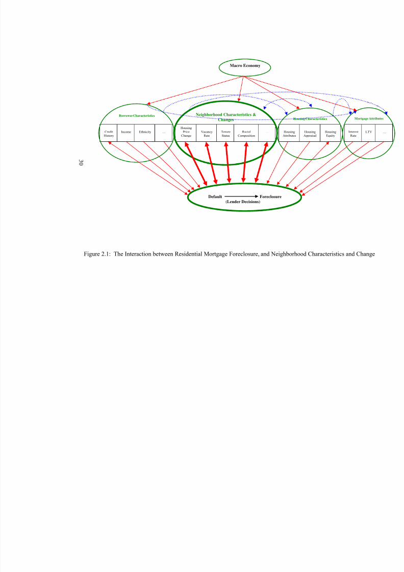
Figure 2.1: The Interaction between Residential Mortgage Foreclosure, and Neighborhood Characteristics and Change............................................................... 30
Figure 3.1: Spatial Regression Decision Process (Anselin, 2005: 217) ........................... 78
Figure 4.1: Judicial Foreclosure Process .......................................................................... 86
Figure 4.2: New Foreclosure Filings in Ohio (1990–2005).............................................. 87
Figure 4.3: Change of Foreclosures Started in Ohio (1984–2003)................................... 89
Figure 4.4: Average Annual Growth Rate of New foreclosure Filings by County .......... 90
Figure 4.5 New Foreclosure Filings in Cuyahoga County and Franklin County (1990– 2004) ................................................................................................................................. 92
Figure 4.6: Research Area: Cuyahoga County and Franklin County, Ohio ..................... 95
Figure 4.7: Franklin County Foreclosure Rate Distribution at the Block Group Level(1997–2004)............................................................................................................ 101
Figure 4.8: Spatial Distribution of Sheriff’s Deeds in Franklin County (1997–2004) ... 103
Figure 4.9: Total Residential Sheriff’s Deeds in Franklin County (1997–2004) ........... 105
Figure 4.10: Comparison between the 1997 and 2004 of the Distribution of Sheriff’sDeeds in Franklin County ....................................................................................... 106
Figure 4.11: Foreclosure Rates by Block Groups in Franklin County (1997–2004)...... 107
Figure 4.12: Connectivity of Block Groups in Franklin County .................................... 109
Figure 4.13: Map of Foreclosure Rate Local Spatial Autocorrelation in Franklin County(1997–2004)............................................................................................................ 113
Figure 4.14: Total Sheriff’s Deeds in Cuyahoga County (1965–2004).......................... 118

8/6/2019 Spatial Lag Regression
http://slidepdf.com/reader/full/spatial-lag-regression 13/268
xii
Figure 4.15: Cuyahoga County Foreclosure Rate Distribution at the Block Group Level(1997–2004)............................................................................................................ 121
Figure 4.16: Spatial Distribution of Sheriff’s Deeds in Cuyahoga County (1997–2004)................................................................................................................................. 122
Figure 4.17: Total Residential Sheriff’s Deeds in Cuyahoga County (1997–2004)....... 124
Figure 4.18: Comparison between the 1997 and 2004 Distribution of Sheriff’s DeedTransfer in Cuyahoga County................................................................................. 125
Figure 4.19: Foreclosure Rates by Block Groups in Cuyahoga County (1997–2004) ... 126
Figure 4.20: Foreclosure Rates by Block Groups in Cuyahoga County (1983-1989).... 128
Figure 4.21: Connectivity of Block Groups in Cuyahoga County.................................. 130
Figure 4.22: Map of Foreclosure Rate Local Spatial Autocorrelation in Cuyahoga County(1997–2004)............................................................................................................ 134
Figure 5.1: Summary of the Interaction between Residential Mortgage Foreclosure and Neighborhood Characteristics and Change............................................................. 191
Figure 6.1: Change in Female Headship Rate in Cuyahoga County (1990–2000, % points)................................................................................................................................. 201
Figure 6.2: Change in Percentage Population below the Poverty Line in CuyahogaCounty (% points) ................................................................................................... 202
Figure C.1: The Local Spatial Autocorrelation between Female Headship Rate in 2000and Foreclosure Rate (2001–2004) in Franklin County ......................................... 217
Figure C.2: The Local Autocorrelation between Median Household Income in 2000 andForeclosure Rate (2001–2004) in Franklin County ................................................ 218
Figure C.3: The Local Autocorrelation between Housing Cost Burden with a Mortgage in2000 and Foreclosure Rate (2001–2004) in Franklin County ................................ 219
Figure C.4: The Local Autocorrelation between Median Housing Value of Owner-Occupied Housing Units in 2000 and Foreclosure Rate (2001–2004) in FranklinCounty..................................................................................................................... 220
Figure C.5: The Local Autocorrelation between Housing Vacancy Rate in 2000 andForeclosure Rate (2001–2004) in Franklin County ................................................ 221
8/6/2019 Spatial Lag Regression
http://slidepdf.com/reader/full/spatial-lag-regression 14/268
xiii
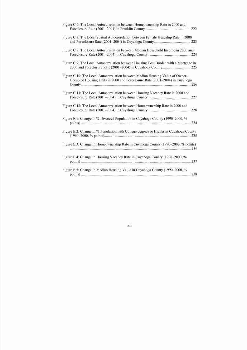
Figure C.6: The Local Autocorrelation between Homeownership Rate in 2000 andForeclosure Rate (2001–2004) in Franklin County ................................................ 222
Figure C.7: The Local Spatial Autocorrelation between Female Headship Rate in 2000and Foreclosure Rate (2001–2004) in Cuyahoga County....................................... 223
Figure C.8: The Local Autocorrelation between Median Household Income in 2000 andForeclosure Rate (2001–2004) in Cuyahoga County.............................................. 224
Figure C.9: The Local Autocorrelation between Housing Cost Burden with a Mortgage in2000 and Foreclosure Rate (2001–2004) in Cuyahoga County.............................. 225
Figure C.10: The Local Autocorrelation between Median Housing Value of Owner-Occupied Housing Units in 2000 and Foreclosure Rate (2001–2004) in CuyahogaCounty..................................................................................................................... 226
Figure C.11: The Local Autocorrelation between Housing Vacancy Rate in 2000 andForeclosure Rate (2001–2004) in Cuyahoga County.............................................. 227
Figure C.12: The Local Autocorrelation between Homeownership Rate in 2000 andForeclosure Rate (2001–2004) in Cuyahoga County.............................................. 228
Figure E.1: Change in % Divorced Population in Cuyahoga County (1990–2000, % points) ..................................................................................................................... 234
Figure E.2: Change in % Population with College degrees or Higher in Cuyahoga County(1990–2000, % points)............................................................................................ 235
Figure E.3: Change in Homeownership Rate in Cuyahoga County (1990–2000, % points)................................................................................................................................. 236
Figure E.4: Change in Housing Vacancy Rate in Cuyahoga County (1990–2000, % points) ..................................................................................................................... 237
Figure E.5: Change in Median Housing Value in Cuyahoga County (1990–2000, % points) ..................................................................................................................... 238

8/6/2019 Spatial Lag Regression
http://slidepdf.com/reader/full/spatial-lag-regression 15/268
1
CHAPTER 1
INTRODUCTION AND RESEARCH QUESTIONS
Residential mortgage foreclosures are the processes that homeowners are legally
forced to foreclose on their properties because they default on their mortgage payment.
There are many factors contributing to foreclosures. Foreclosures have profound impacts
on individual homeowners, neighborhoods, mortgage lenders, and policies. As the first
step of a research agenda this project focuses on the interaction between residential
mortgage foreclosures, neighborhood characteristics, and neighborhood change.
Residential mortgage default and foreclosure issues did not attract much attention
until the mid 1970s, when the single-family foreclosure rate in the U.S. began to increase.
Most of the studies since then focused on the factors contributing to mortgage default and
foreclosure, with an emphasis on what financial institutions could do better to manage
their credit risk (Quercia and Stegman, 1992). Since 2000, there has been a dramatic rise
in foreclosure rates, especially in Ohio and Indiana, and it has caused great concern
among policy makers, citizen advocacy groups, fair housing agencies, and other
concerned individuals. This means that many more stakeholders are showing an interest
in mortgage default and foreclosure. The complexity of this issue has increased with the
advent of flexible financial products, along with increasing ethical and legal challenges
8/6/2019 Spatial Lag Regression
http://slidepdf.com/reader/full/spatial-lag-regression 16/268
2
facing the real estate profession (such as mortgage fraud, incomplete disclosure of costs
associated with mortgages, using a “teaser rate” to confuse loan borrowers, etc.).
Nature of the Problem
There is abundant literature on factors contributing to mortgage default and
foreclosure. Many of the previous studies focused on measuring default risk using
various factors and models, in order to provide more accurate mortgage pricing and risk
management for financial institutions. Neighborhood characteristics are one of the
important sets of factors that should be considered in these models of residential
mortgage foreclosure. But only a few scholars have paid attention to the impact of
neighborhood characteristics on residential mortgage foreclosure (Cotterman, 2001; von
Furstenburg and Green, 1974; Williams et. al., 1974; Sandor and Sosin, 1975).
Residential mortgage foreclosure is an issue in housing markets, and housing
markets are geographically bounded. So mortgage foreclosure, neighborhood
characteristics and neighborhood change are related to each other in complex ways. But,
just as with the studies of neighborhood effects on mortgage default and foreclosure, the
impacts of foreclosure on neighborhood characteristics and change have not been fully
explored, with the notable exception of the studies conducted by Lauria and Baxter in
New Orleans (Lauria, 1998; Lauria and Baxter, 1999; Baxter and Lauria, 2000), and
Immergluck and Smith in Chicago (Immergluck and Smith, 2005a, 2005b).
The interaction between mortgage foreclosure and neighborhood change is very
complicated and is related to many different aspects of housing market equilibrium,
economic development, lender and borrower decision theory and social transition, among
8/6/2019 Spatial Lag Regression
http://slidepdf.com/reader/full/spatial-lag-regression 17/268
3
other things. In order to examine the interactive relationships between residential
mortgage foreclosure and neighborhood characteristics and change, this study uses
Sheriff’s foreclosure sales data in the two most populous counties in Ohio, Cuyahoga
County and Franklin County, the central counties of the Cleveland and Columbus
metropolitan areas, respectively.
Ohio has one of the highest residential mortgage foreclosure rates in the United
States, where the foreclosure rate is defined as the number of mortgages in foreclosure as
a percentage of all mortgage loans outstanding (Krumkin, 2000). There has been a
tremendous increase in foreclosures in Ohio since 1995. These two Ohio counties provide
good case studies for testing hypotheses about the interaction between mortgage
foreclosure and neighborhood characteristics and change. The Sheriff’s Sales data are
combined with other datasets, such as census demographic data, housing and economic
data, and real property parcel data in each county, to develop a deeper understanding of
the complexities than has been previously available (Cotterman, 2001; Baxter and Lauria,
2000).
Objective of the Research
The objective of this research is to improve our understanding of the complex
relationship between neighborhood characteristics, foreclosure and neighborhood change.
In addition, I hope to make a significant contribution to housing and foreclosure policy in
Ohio. The findings will contribute to both theory and policy on foreclosure and
neighborhood change. The research results will also help target community-based
foreclosure prevention programs to the most at-risk neighborhoods. The document
8/6/2019 Spatial Lag Regression
http://slidepdf.com/reader/full/spatial-lag-regression 18/268
4
includes suggestions for ways to intervene to reduce foreclosure concentration and the
impacts of such concentration on neighborhoods. The research will contribute to the
limited academic literature on this topic by adding significant work over time and across
space, allowing an analysis of the context within which foreclosure occurs. The explicit
consideration of racial issues and the problem of house price depreciation incorporated in
this analysis will also enhance the existing models.
Research Questions
There are three primary questions that the research tries to answer. Following each
question are more detailed hypotheses.
1. Do neighborhood characteristics and changes affect residential mortgage default and
foreclosure? If so, how?
If the answer to this question is yes, several subsidiary questions need to be
addressed. For example, what neighborhood factors contribute to mortgage default risk
and rising mortgage foreclosure rates? What kinds of neighborhoods have seen the
highest increase in foreclosure sales? Why do different neighborhoods have different
foreclosure rates? Do the phenomena follow certain patterns over time in different
metropolitan areas?
2. Do mortgage foreclosures affect neighborhoods? How and under what circumstances?
According to previous research, mainly by Lauria and Baxter (1998, 1999, 2000),
the impact of mortgage foreclosure on neighborhoods in which foreclosed properties are
8/6/2019 Spatial Lag Regression
http://slidepdf.com/reader/full/spatial-lag-regression 19/268
5
located is very significant. They found important impacts on racial transition and general
economic condition of the neighborhoods.
Properties in some neighborhoods tend to have a lower price appreciation (Oliver
and Shapiro, 1995; Raffalovich, 2002; Shapiro, 2004), which in turn makes it more likely
that people will default on mortgages because a lower appreciation rate or depreciation
will decrease the property’s real value, and that leads to less equity. If values depreciate
enough, the property could end up with negative equity. Negative equity is one of the
leading reasons for people to default on mortgage payments (Case and Shiller, 1996;
Cunningham and Capone, 1990). Higher foreclosure rates in a neighborhood can
decrease housing values in the neighborhood and make price appreciation even lower,
thus making more people likely to default. On the other hand, the characteristics of the
residents of these neighborhoods must also be taken into account as those characteristics
could tend to lead to higher default rates. Thus, the complexity of the geographic
relationships, as well as the interdependencies of the people and the neighborhoods,
requires special attention. In this research, in addition to the racial composition and
general economic condition of neighborhoods, housing price appreciation and other
housing stock characteristics of neighborhoods are explored to find out whether and how
mortgage foreclosure affects housing price appreciation and neighborhood stability.
3. Can we model the cyclical nature of the relationship between neighborhood
characteristics, neighborhood change and foreclosure rates?
The first two research questions indicate that separating the impact of
neighborhoods on foreclosures from the impact of foreclosures on neighborhoods is a
8/6/2019 Spatial Lag Regression
http://slidepdf.com/reader/full/spatial-lag-regression 20/268
6
crucial methodological problem. Thus, in order to address these two substantive
questions, the research must address the methodological question that is relevant to many
neighborhood-effects studies. Neighborhood-effects research is a controversial area of
inquiry in social sciences (Dietz, 2002), although there is abundant literature addressing
research methods in the area. There are several difficult problems in this area of research,
including endogenous effects, omitted variables, and reflection problems (Dietz, 2002;
Manski, 2001). My research develops a model to deal with the nonrecursive nature of the
relationship between neighborhood characteristics, neighborhood change and foreclosure
rates, taking into account the possibility of endogenous effects, omitted independent
variables and the reflection problem (Dietz, 2002).
Scope of the Research
The major datasets used for this research are the Sheriff’s deed transfer data from
1997 to 2004 (in Cuyahoga County the data from 1983 to 1989 are also used), the census
block group data from 1990 and 2000, the census designated place data from 1990 and
2000, and real property parcel data from 2004 and 2005. These datasets were merged for
analysis purposes. More details in the data sets and the methodologies are included in the
relevant chapters. The second chapter of this dissertation provides the literature review
and conceptual models. Then I turn to the results.
The first section of results provides the descriptive and spatial analyses of the
foreclosure patterns in each county, and their relationships with selected neighborhood
characteristics.
8/6/2019 Spatial Lag Regression
http://slidepdf.com/reader/full/spatial-lag-regression 21/268
7
The second results section reports the outcomes of the advanced spatial analysis and
the spatial modeling. Spatial autocorrelation analysis measures how spatial
autocorrelation affects the regression results and how the spatial lag and error models
differ from the Ordinary Least Square (OLS) regression models when using
neighborhood variables to predict foreclosure rate.
The third section of the results formulates a Seemingly Unrelated Regression (SUR)
system to measure how foreclosure rates and other neighborhood and place-characteristic
variables affect each selected neighborhood change variable in each county.
In the final chapter of the dissertation, the major findings from the research will be
used as the basis for policy suggestions to help policy makers be aware of the spatial
patterns of foreclosure, the mutual impact of neighborhood variables and foreclosure, and
the specific neighborhood factors that are highly related to foreclosure. Targeted policies
can be created to manage neighborhood variables identified in this research in order to
break the cyclic nature of the relationship between neighborhood characteristics and
foreclosure. The establishment of spatial analysis and models and SUR models in the
research will provide an effective method for analyzing similar research questions, and
the combination of these spatial and quantitative models will contribute to foreclosure
research.
8/6/2019 Spatial Lag Regression
http://slidepdf.com/reader/full/spatial-lag-regression 22/268
8
CHAPTER 2
LITERATURE REVIEW
Residential Mortgage Foreclosure
Concepts of Mortgage Delinquency, Mortgage Default and Foreclosure
Mortgage foreclosure is “the process by which the mortgage originators claim legal
rights to the property by foreclosing the mortgage in the event of mortgage default”
(Frumkin, 2000). A mortgage delinquency, which usually means a mortgage repayment is
overdue 30 days or more, becomes a mortgage default when it is overdue by more than
90 days. When the mortgage is in default, the lender may choose to work with the
borrower to see if the loan can be modified or brought back to a normal balance. When
these efforts fail, the lender will usually file a foreclosure with the court to claim its legal
rights under the mortgage. Many studies treat “default” and “foreclosure” as synonymous
(Goering and Wienk, 1996), but in fact, default is incurred and affected by borrowers’
choices, while foreclosure is one of the options available to lenders to enforce the
repayment of a mortgage in default. This research will treat default and foreclosure as
two related but different processes.
A civic real estate sale is the final procedure in a judicial foreclosure process. The
property can be withdrawn from this process if the borrower(s) file for bankruptcy, bring
8/6/2019 Spatial Lag Regression
http://slidepdf.com/reader/full/spatial-lag-regression 23/268
9
the back payments up to date, sell the property, legally cancel the mortgage, or resume
the mortgage repayments.
In contemporary U.S. society, with its mature financial markets and innovative and
flexible financial products, buying a home has become much easier. Homebuyers do not
need to accumulate large amounts of savings in order to purchase a house. When certain
conditions are met, they can readily obtain a mortgage to finance a home purchase,
although different financial agencies might have different underwriting standards.
When a borrower obtains a mortgage to buy a house, a scheduled repayment of the
mortgage is incurred. This schedule is determined by the loan-to-value ratio, loan term,
mortgage interest rate, and interest compounding factors. But the mortgage performances
of borrowers differ greatly and are related to the differences in household characteristics,
such as income, family structure, and mobility decisions, and to the general economic
context, including recessions, interest rates and so forth. Mortgage performance includes
timely submission of mortgage payments, prepayment behavior, refinancing behavior,
mortgage delinquency and mortgage default. Of these behaviors only mortgage
delinquency and default are related to a possible change of homeownership status of
borrowers and the risk of borrowers losing their homes if they are not able to resume the
mortgage repayment.
Mortgage delinquency usually means missing one scheduled payment. At that time,
lenders cannot tell whether the payment will be continued or stopped in the next payment
cycle. But if several payments are missed, usually three (Quercia and Stegman, 1992),
lenders will consider borrowers to have defaulted. The criteria that determine a default
vary among financial institutions. When a loan defaults, lenders will choose either to use
8/6/2019 Spatial Lag Regression
http://slidepdf.com/reader/full/spatial-lag-regression 24/268
10
loss-mitigation techniques to work with the borrowers to resolve the issue and resume the
payments, or foreclose the mortgage by auctioning the mortgage property to cover the
loan balances of the borrowers (Capone Jr., et. al., 1996). Lenders choose the option that
costs the least to process. If the costs of working out the troubled loan are much larger
than foreclosure costs, lenders prefer to choose foreclosure. On the other hand, many
lenders are willing to work with borrowers first to find ways to resolve the issue. If this
cooperation fails, a foreclosure action will be filed in the local civic court or a non-
judicial trustee’s sales process will be initiated. A civic real estate sale is the final
procedure in a judicial foreclosure process.
The decision of whether to choose foreclosure depends greatly on state legislation
(Clauretie, 1987). In a non-judicial process, when loans are in default a notice of default
will be issued to the borrower. Then, if the borrower cannot repay the back payments, a
trustee’s sale will be initiated to sell the foreclosed properties. Thus a non-judicial
foreclosure does not need the involvement of courts and Sheriff’s Offices. But the
judicial process starts with foreclosure filings to the local court. Then, if the borrower
cannot walk out of the foreclosure process (e.g. cannot sell the property before the
auction, or get a bankruptcy), the court will order a Sheriff’s sale. Both judicial and non-
judicial processes have advantages and disadvantages. The biggest advantage of the
judicial process is the legal guarantee that helps the involved parties avoid disputes in
titles and other real estate claims. However, judicial foreclosure is much more expensive
in terms of legal fees and is more time consuming than non-judicial processes. Many
states in the U.S. allow both judicial and non-judicial processes, but Ohio only allows a
judicial process (see Appendix A for a detailed description of the process).
8/6/2019 Spatial Lag Regression
http://slidepdf.com/reader/full/spatial-lag-regression 25/268
11
According to research conducted by Clauretie (1987), states without judicial
foreclosure usually see a higher foreclosure rate because of the low foreclosure costs,
controlling the time span of the foreclosure process. This makes Ohio’s high foreclosure
rate even more surprising.
Previous Research on Mortgage Default and Foreclosure
Studies on residential mortgage default have changed over time. Many have focused
on lenders’ and financial institutions’ need to understand the mechanisms in mortgage
default. Using these studies, financial institutions have sought to minimize mortgage
default risk and losses associated with the risk. Only in recent years has research on the
social impacts of mortgage default and foreclosure begun to appear in the academic
literature. But the recent research still has not resolved some essential issues related to
foreclosure, such as whether there are racial differences in mortgage default decisions,
how and where the households move after they lose their homes due to the foreclosure
process, and how those changes affect the structure of a neighborhood.
Three Generation’s Research on Mortgage Default
In the early 1990s, Quercia and Stegman (1992) summarized the literature on
residential mortgage default. They provided a comprehensive analysis of mortgage
default risk from three different perspectives, that of lenders, borrowers, and institutions,
each of which is associated with a research generation. These perspectives have
contributed to the mortgage default literature either theoretically or empirically. Their
research also tried to seek different indicators to measure mortgage default risk, such as
8/6/2019 Spatial Lag Regression
http://slidepdf.com/reader/full/spatial-lag-regression 26/268
12
default rates, expected mortgage losses, and interest rate premiums (Quercia and
Stegman, 1992).
The first generation’s studies were from the lender’s perspective. Minimizing credit
risk is one of the essential activities in the daily management of financial institutions
(Saunders and Cornett, 2003). The goal of lenders facing mortgage default by borrowers
is to lower the costs associated with defaults and foreclosures. This stream of research
found that mortgage default rates are correlated with loan characteristics, borrower
characteristics and property characteristics. For example, loans with higher loan-to-value
ratios, higher interest rates and longer terms are much more likely to be in default
compared to the reverse characteristics of those indicators. Higher initial payment-to-
income ratio, properties with poor conditions and unstable neighborhoods usually are also
associated with a higher default risk.
The second generation’s research was from the borrower’s perspective and probed
borrower payment models. The models are based on utility (net wealth) optimization in
consumer theories and option-based choices. The utility (net wealth) optimization
theories indicate that when borrowers make decisions (timely payment, prepay, refinance,
or default) in their mortgage performance they base those decisions on the maximization
of their net wealth. The option-based models view default as a put option, where the
borrowers can sell the property back to the lender for the value of the mortgage at the
beginning of each payment period. Those mortgage performance choices are determined
by many factors, such as transaction costs, family crises and mobility decisions.
The third generation’s research was from the perspective of large financial
institutional loan pools and financial regulators. The research explored, for example, how
8/6/2019 Spatial Lag Regression
http://slidepdf.com/reader/full/spatial-lag-regression 27/268
13
default happens on an FHA-insured mortgage or on a fixed-interest mortgage, and how
some regulations (e.g., capital requirements) affect mortgage default. But the studies of
the third generations are more complete and have considered the roles of all three sectors:
lenders, large financial institutions and regulators, and borrowers.
Quercia and Stegman concluded that there are still some obstacles in the research.
One of the greatest is the lack of data about changes to borrower, lender and property
information over time, which limits the research to some extent. But the most difficult
problem is the lack of data about borrower’s issues and decisions. They also indicate that
mortgage default models need to incorporate not only the role of borrowers but also the
mobility decision of borrowers.
Mortgage Default and Foreclosure Factors
There are many factors determining the possible mortgage default risk of certain
loans, but loan-to-value ratio, payment-to-income ratio, householder’s occupation (with
or without volatile income), property and neighborhood condition, regional
unemployment rate, transaction costs, crisis events, and borrowers’ expectations are some
of the major elements contributing to the risk of mortgage default and foreclosure
(Quercia and Stegman, 1992; HUD, 1992; Vandell and Tribodeau, 1985).
Among those factors, the macro economic situation, housing price appreciation and
neighborhood characteristics are macro spatial factors that help determine borrower
characteristics in certain geographical areas and, therefore, the loan characteristics
associated with those borrowers. Using those factors, loan default risk in certain
geographical areas can be measured. According to previous literature on mortgage default
8/6/2019 Spatial Lag Regression
http://slidepdf.com/reader/full/spatial-lag-regression 28/268
14
and foreclosure, the following is a list of major factors contributing to mortgage default
and foreclosure, although some of them are correlated to others:
• Macro economic situation
• Mortgage loan characteristics
• Types of Mortgage Products
• Borrower characteristics and default decisions
• Mortgage lending legislation and foreclosure legislation
• Lender decisions in mortgage foreclosure
•
Housing attributes
• Housing appraisal
• Housing price appreciation
• Mortgage fraud
• Neighborhood characteristics.
I will discuss each of these briefly, though they are not the focus of this dissertation.
Macro economic situation
Studies have found that mortgage default is largely related to macro economic
changes over time. The most obvious indexes that are associated with mortgage default
are the unemployment rate, interest rate, and housing price index.
Bellamy (2002) found that in Ohio between 1994 and 2001 the unemployment rate
fell consistently, with minor volatility, but foreclosure filings increased consistently.
Therefore, he suggested that the increasing foreclosure rates in Ohio are not solely
dependent on the economic situation. A report from Policy Matters Ohio in 2004 assumes
8/6/2019 Spatial Lag Regression
http://slidepdf.com/reader/full/spatial-lag-regression 29/268
15
a weak economy since 2001 to be one of the leading reasons for the high foreclosure rate
in Ohio in recent years. Case and Shiller (1996) found that high mortgage default rates
“strongly follow” real estate price declines or interruptions of real estate price increases.
Also, mortgage delinquency and foreclosure rates themselves are important economic
indicators (Frumkin, 2000).
Mortgage Loan Characteristics
Loan characteristics are important factors that can affect mortgage defaults and
foreclosures. In early research there were many interesting findings, such as that the
interest risk is one indicator of mortgage risk, and a higher loan-to-value ratio means
more default risk.
Many studies found that the initial loan-to-value (LTV) ratio has a significant
influence on mortgage default (Von Fustenberg, 1969, 1970a, 1970b; Deng and Gabriel,
2002; Calhoun and Deng, 2002; Ambrose et. al. 2002). The LTV ratio directly
determines the equity position of a borrower (HUD, 2004), and HUD found that a high
LTV ratio is associated with a high default rate by examining FHA-insured and GSE
(Government Sponsored Enterprises: Fannie Mae, Freddie Mac and Ginnie Mae)-
purchased loans. Von Furstenberg (1969, 1970a, 1970b) thought that home equity at the
time of loan origination is highly related to mortgage default. When the LTV ratio is
raised by seven percentage points from 90% to 97%, default rates for new homes increase
by seven times. But research found that in subprime mortgages the LTV has little effect
on loan performance (OCC, 2003). Quercia et.al. found that LTV ratio does not affect
8/6/2019 Spatial Lag Regression
http://slidepdf.com/reader/full/spatial-lag-regression 30/268
16
default in their panel data of rural low-income mortgage borrowers (Quercia et. al.,
1995).
Interest rates that financial institutions charge to loan borrowers reflect the
expectations from the lenders about default potential. The lenders are hedging possible
losses from credit risk, so interest rate should be related to mortgage default risk (Jung,
1962). The yield curve slope therefore should be a factor contributing to mortgage
defaults (HUD, 2004). This hypothesis was later proven by other research. For example,
Page (1964) found that default risk was related to property values; financial institutions
are willing to issue loans with a lower interest rate to borrowers purchasing a high-value
property. A borrower who caught a loan to buy an expensive house probably has good
credit so their interest rate is low. In a situation of burnout1, where borrowers passed up
some previous good opportunities to refinance the mortgage at a more favorable interest
rate, they have a higher tendency to default because of the high interest rates (HUD,
2004). Ambrose and Sanders (2003) also found that the change in yield curve has a direct
impact on the probability of mortgage default.
Besides interest rates and LTV ratios, loan term length and the age of the mortgage
are also important factors (von Furstenberg, 1969). Von Furstenberg (1969) found that
mortgage default risk positively correlates with the term of the mortgage and a mortgage
younger than 3 or 4 years is at higher risk as well.
HUD (2004) found that loan size is also a factor in determining loan default risk by
exploring both PMI (Private Mortgage Insurance) and FHA loan data. Smaller loan sizes
usually are associated with a higher default rate, which might be because that low-income
borrowers, low-liquid-asset borrowers, or borrowers with high income-volatility tend to
8/6/2019 Spatial Lag Regression
http://slidepdf.com/reader/full/spatial-lag-regression 31/268
17
have smaller loans. That can also indicate high housing price volatility in low-priced
houses.
Quercia and Stegman (1992) stated that default patterns for adjustable rate
mortgages (ARMs) were not comprehensively studied before. With ARMs, payment
shock due to unexpected interest rate increase is one of the important reasons for people
to default. Early ARM payment accounts for the impact of the change of payment coupon
from an initial low rate (“teaser rate”) to an index-adjusted rate during the first year of the
loan. Therefore, early ARM payment can also explain some of the default risk.
Another factor contributing to mortgage delinquency and default is the presence and
holding status of junior or subordinate loans and liens (Herzog and Earley, 1970; LaCour-
Little, 2004). Their research found that junior or subordinate loans and liens might
increase the default risk of primary loans.
Types of Mortgage Products
Product types such as FHA-insured, VA-insured, Conventional, ARM, FRM (Fixed
Rate Mortgage), GRM (Graduated Rate Mortgage) and subprime loans affect mortgage
default risk due to their own characteristics. According to the Mortgage Bankers’
Association, FHA loans usually have a higher foreclosure rate than conventional
mortgages. But determinants of delinquency rates in different types of loans are different,
especially for some non-profit community lending organizations in which social
networks, business culture, funding sources, composition of the board and loan
committees, staff structure, loan intake, and collection tools are major organizational
factors affecting loan delinquency rate (Baku and Smith, 1998).
8/6/2019 Spatial Lag Regression
http://slidepdf.com/reader/full/spatial-lag-regression 32/268
18
The role of subprime and predatory lending on increasing mortgage foreclosures is
addressed by many previous studies and in different states such as Ohio, Indiana and
Arizona (Realtors, 2003; Goldstein, 2004; Rhey and Posner, 2004; Stock et. al., 2001). A
study of the differences in mortgage default rates of prime and non prime mortgages
indicates that these mortgages are significantly different in many aspects, such as
different risk levels at the loan origination. They both default at elevated levels but
respond differently to incentives to prepay or default (Pennington-Cross, 2003). The
study also found that mortgage default is less responsive to the amount of equity when
credit scores are included in the analysis.
Borrower Characteristics and Default Decisions
Default decisions made by borrowers are determined by many factors. A default is
usually due to two situations: inability to pay and/or unwillingness to pay. Those two
scenarios should be separated when exploring mortgage default decisions. In addition to
factors described in the preceding section on borrower characteristics in mortgage default
risk models, certain events such as changes in borrower characteristics and life crises can
also make borrowers choose default. The most important such factors are job loss, family
structure change (such as divorce, children going to college, or decease of a financially
supportive adult), and moving.
When terminating a mortgage, the decision of a household to default is determined
by the borrower’s perception of the value of the mortgage versus the value of the home.
When the house is perceived to be less valuable than the outstanding mortgage balance, a
decision to default might be made and this is a voluntary default decision. Another
8/6/2019 Spatial Lag Regression
http://slidepdf.com/reader/full/spatial-lag-regression 33/268
8/6/2019 Spatial Lag Regression
http://slidepdf.com/reader/full/spatial-lag-regression 34/268
20
and credit history on mortgage default risk, recent research has begun to focus more on
comprehensive loan characteristics, borrower characteristics, and property and
neighborhood characteristics.
The payment-to-income ratio is thought to have a significant effect on mortgage
default, but empirical studies show mixed results. Therefore, we cannot say that its
impact on mortgage default is significant (HUD, 2004).
Earlier research found that the effect of income on mortgage default was ambiguous
(HUD, 1992). However, Van Order and Zorn (2002), in a recent study of competing risk
of mortgage termination, found that borrower income is an important determinant for
mortgage default decisions when the borrower’s property has negative equity. Although
few studies have focused on income levels, many have tried to examine the impact of
income variability (stability and growth) on mortgage default. Van Order and Zorn
(2002) also found a positive relationship between income variability and the mortgage
default rate. This means that high volatility of income is usually associated with a high
default rate. Borrowers with certain occupations, such as those who are self employed,
those whose major income depends on commissions, and those with low-skilled jobs
(HUD, 2004), have high income volatility. Research also found that borrowers with low
liquid assets have a higher mortgage default probability (HUD, 2004).
In several studies the impact of a borrower’s ethnic background was greatly reduced
by controlling other characteristics, such as down payment and credit history (Cotterman,
2002; Van Order and Zorn, 2002). Therefore, many researchers believe that loan default
differences among different racial groups can be better explained by down payment
amount and credit history of the borrowers. Some think that racial minorities are more
8/6/2019 Spatial Lag Regression
http://slidepdf.com/reader/full/spatial-lag-regression 35/268
21
likely to become targets of predatory lending, but little attention has been paid to possible
racial disparities in mortgage performances, mortgage default and mortgage foreclosures.
Only in recent years have some scholars noticed this issue (Lauria and Baxter, 1999;
Lauria, 1998; Baxter and Lauria, 2000).
Mortgage default will affect the future credit worthiness of a borrower. But for some
borrowers, repeated mortgage decisions can be observed. Ambrose and Capone (2000)
found that borrowers with a first default have a greater risk for a second default, and the
risk is also greater when the time difference between two defaults is shorter than two
years. They also found that the economic factors affecting the first default have no effect
on the second default. The findings of this study imply that the ability of borrowers to
obtain another mortgage will be lower since they have been found to have a higher
default probability in their second mortgage.
Mortgage Lending Legislation and Foreclosure Legislation
The impact of mortgage lending legislation on foreclosure is under-investigated
because of the difficulty of evaluating how legislation contributes to foreclosure. But
recently, with the increasing awareness of mortgage foreclosure, some non-profit
organization and concerned citizen groups have begun to question whether loose
mortgage lending legislation and regulations are an important factor affecting
foreclosure. They might especially affect the geographically clustered distribution of
foreclosure in low-to-moderate-income neighborhoods. The major agenda that these
groups propose is to enact anti-predatory lending legislation and require real estate and
mortgage brokers/agents and real estate appraisers to pass stricter licensing exams. At the
8/6/2019 Spatial Lag Regression
http://slidepdf.com/reader/full/spatial-lag-regression 36/268
8/6/2019 Spatial Lag Regression
http://slidepdf.com/reader/full/spatial-lag-regression 37/268
23
State bankruptcy laws also have some impact on default decisions of borrowers. Lin
and White (2001) found that in states with higher bankruptcy exemptions borrowers have
greater tendencies to choose default.
Lender Decisions in Mortgage Foreclosure
There are three possible outcomes when a mortgage is defaulted: (1) resumption of
payments, (2) termination by prepayment, or (3) foreclosure (Phillips and VanderHoff,
2004). The value of termination options and local economic and housing market
conditions affect default resolution probabilities greatly. After a study of loan pools in a
large national savings and loan institution, Phillips and VanderHoff (2004) found that
judicial procedure and tenancy statutes decrease the probability of foreclosure by 25%,
due to the increasing costs of foreclosure. They also indicate a possibility of adjusting
mortgage rate premiums to compensate the added costs to lenders.
For FHA-insured loans, lenders do not bear many foreclosure costs when
foreclosures occur (Realtors, 2003). This could be one of the reasons why FHA loans
have a high foreclosure rate.
The amount of time between mortgage default and foreclosure is different
depending upon the mortgage interest rate and home equity values (Lauria, 2004). Lauria
found that lower interest rate loans and loans with an outstanding balance below the
median value of the home were given a longer time from default to foreclosure. Whether
there is racial discrimination in the foreclosure process is still unclear.
8/6/2019 Spatial Lag Regression
http://slidepdf.com/reader/full/spatial-lag-regression 38/268
24
Housing Attributes
Housing attributes, such as the number of bedrooms in a dwelling and the units in
the building, building type, and building year, are important factors in loan approval in
the automated mortgage scoring system of many types of mortgages, and this is where
home equity values could go. Therefore they can be important indirect factors affecting
mortgage default risk (Sandor and Sosin, 1975).
Housing Appraisal
In research on the role of real estate appraisal on mortgage lending and performance
in Alaska’s housing market, Lacour-Little and Malpezzi (2003) found that if the appraisal
value of a property is higher than the estimated price from a hedonic model they
developed, the mortgage against this property is exposed to more default risk. In other
research, Lacour-Little and Green (1998) found that minorities and minority
neighborhoods are much more likely to get low appraisals, which increases the loan
application rejection rates of racial minorities. But they found that the low appraisal is
related to poor neighborhood and housing quality. Noordewier et. al. (2001) found that
properties with a higher appraisal value than similar recently sold properties are related to
higher default risk of the borrowers.
Housing Price Appreciation
Housing price change is a very important factor in determining mortgage default
probabilities. This is true, first, because of the possibility of negative equity, which
affects mortgage default decisions greatly (Quigley et. al., 1993), is largely determined by
8/6/2019 Spatial Lag Regression
http://slidepdf.com/reader/full/spatial-lag-regression 39/268
25
housing price changes (Case and Shiller, 1996). Second, as housing prices fall, the loss
severity followed by a default increases, and loss severity increases non-linearly and
faster than the decline of housing prices (Case and Shiller, 1994). Third, the research on
housing price appreciation in low-income and/or minority neighborhoods should help
explain the disparities among mortgage foreclosure rates in different neighborhoods
(Raffalovich, 2002). By examining neighborhood effects on FHA-insured loans,
Cotterman (2001) found that low housing price appreciation in minority neighborhoods is
an important factor in the higher default rates in those neighborhoods.
Housing price appreciation is also an important motivation for people to move
(Kiel, 1993). When a moving decision is made, borrowers will choose either to sell or
default on the property in which they currently reside (Pavlov, 2001). When the equity
value is positive they will usually choose to sell the property and prepay the mortgage.
But when the equity value is negative and cannot offset default costs, they will choose to
default. However, only a small percentage of borrowers actually choose to default in this
situation. Their decision might be more determined by life crisis events because choosing
default is costly for borrowers in regard to its negative impact on borrower credit scores
(HUD, 1992; Foster and Van Order, 1985).
Mortgage Fraud
Foreclosure cases because of mortgage fraud are few and there is no literature
related to the relationship between mortgage fraud and foreclosures. Hence there are no
empirical studies conducted to see how mortgage fraud affects foreclosure. The definition
of mortgage fraud can be very broad, but here it means that lenders use some illegal
8/6/2019 Spatial Lag Regression
http://slidepdf.com/reader/full/spatial-lag-regression 40/268
8/6/2019 Spatial Lag Regression
http://slidepdf.com/reader/full/spatial-lag-regression 41/268
27
and other minorities are required to have a higher standard than Whites in loan approval,
and thus Blacks and other minorities have a lower tendency to default because those who
can have a loan are those who meet the higher standards; also “minorities tend to have
less attractive distributions of factors leading to default” compared to whites because of
the more strict underwriting standards (Cotterman, 2004). But a study by Berkovee et. al.
(1994, 1995) found that black homeowners have a higher default rate than white
homeowners, which contradictorily indicates that mortgage default has no relationship to
lending discrimination. Anderson and VanderHoff (1999) also found that Black
homeowners have a higher marginal default rate than white households, controlling for
borrower and property characteristics. Other scholars found that there are flaws with
using mortgage default to predict mortgage lending discrimination (Ross, 1996;
Anderson and VanderHoff, 1999). Controlling credit history reduces the effect of races
on mortgage default (Cotterman, 2002). Deng and Gabriel (2003) and Van Order and
Zorn (2001) found that minorities have higher default probabilities, but the losses from
their high default risk can be offset by their low tendency for prepayment. They
recommend that financial institutions should have similar pooling and risk-based
mortgage pricing for all borrowers, which will benefit more racial minorities and
therefore improve their homeownership rate. Cotterman (2004) concluded that Blacks
and Hispanic borrowers incur a larger loan loss rate than Whites in FHA-insured loans,
but he did not explore whether the loss could be offset by the lower prepayment tendency
of racial minorities.
Therefore, many researchers think that racial disparities in mortgage default can be
explained by other factors, such as down payment amount and credit history, which
8/6/2019 Spatial Lag Regression
http://slidepdf.com/reader/full/spatial-lag-regression 42/268

8/6/2019 Spatial Lag Regression
http://slidepdf.com/reader/full/spatial-lag-regression 43/268
8/6/2019 Spatial Lag Regression
http://slidepdf.com/reader/full/spatial-lag-regression 44/268
3 0
Figure 2.1: The Interaction between Residential Mortgage Foreclosure, and Neighborhood Characteristi
Macro Economy
CreditHistory
Income Ethnicity …Housing
PriceChange
VacancyRate
TenureStatus
RacialComposition
… HousingAttributes
HousingAppraisal
HousingEquity
Default Foreclosure
(Lender Decisions)
Neighborhood Characteristics &
Changes Housing CharacteristicsBorrower Characteristics
8/6/2019 Spatial Lag Regression
http://slidepdf.com/reader/full/spatial-lag-regression 45/268
31
The Interaction between Neighborhood Characteristics, Neighborhood
Change and Residential Mortgage Foreclosure
General Theories of Neighborhood Change
As mentioned earlier, the development of neighborhood change theory can be
summarized into three generations and research concentrations (Galster and Krall, 2003).
Because these generations have temporal overlap, it is not appropriate to conclude that
they have specific temporal orders. Many contemporary scholars still use the theories
formulated in the first generation in their research. Many conduct their research on
neighborhood change based on the theories of one of the three generations, or the
combined theories from two or three generations.
1. The first generation: descriptive, cartographic and causal analysis (1950 – )
Simple descriptive, cartographic and causal analysis dominates in this generation.
The major theoretical bases are the invasion-succession model that was proposed by the
Chicago School of Sociology (Park, 1952; Duncan and Duncan, 1957; Taeuber and
Taeuber, 1965), the life-cycle model (Hoover and Vernon, 1959), the
demographic/ecological model, the social-cultural/organizational model, the social
movement model (Downs, 1981; Bradbury, et. al., 1982; Schwirian, 1983), the stage
model, and the political-economy model. These theories have been followed by
Maclenna(1982), Taub, et. al. (1984), Grigsby, et. al. (1987), Rothenburg et. al. (1991),
Temkin and Rohe (1996), Lauria (1998), and Galster (2003). All these theories have
formed the fundamental basis of neighborhood change theory by describing how
neighborhoods change, the push and pull factors of the change, and what factors are
affected the most in the neighborhood-succession process. Some of the theories use
8/6/2019 Spatial Lag Regression
http://slidepdf.com/reader/full/spatial-lag-regression 46/268
32
mechanisms in other disciplines, for example, ecology, to explain the dynamic processes
of a neighborhood. This research will use some of the aforementioned methodology, such
as cartography and descriptive and causal analysis to explain how foreclosures and
neighborhood characteristics and change interact with each other. Some of the terms
developed in this generation, such as racial transition and exogenous variables, will be
used extensively in this research.
2. The second generation: regression and predictive models (1970 – )
Regression and predictive models are used to explore how exogenous variables
affect neighborhood outcome indicators and estimate-related indicators (Galster and
Krall, 2003). Examples of those indicators are population density (Guest, 1972, 1973;
Fogarty, 1977), income or social class (Guest, 1974; Vandel, 1981; Coulson and Bond,
1990; Galster and Mincy, 1993; Galster et. al., 1997; Carter et. al., 1998),
homeownership rate (Baxter and Lauria, 2000), female headship rates (Krivo et. al.,
1998), and racial composition changes (Guest and Weed, 1976; Schwab and Marsh,
1980; Ottensmann et. al., 1990; Galster, 1990; Denton and Massey, 1991; Ottensmann
and Gleeson, 1992; Lauria and Baxter, 1999; Crowder, 2000; Ellen, 2000; Baxter and
Lauria, 2000). There are mixed findings in the studies, but all these indicators provided
the basis for this research when selecting variables. Similarly, when exploring the impact
of foreclosure on neighborhood characteristics and change, foreclosure rate is the
exogenous variable that affects the neighborhood indicators and their change. Only a few
scholars have paid attention to this matter. This research will also use regression and
8/6/2019 Spatial Lag Regression
http://slidepdf.com/reader/full/spatial-lag-regression 47/268
33
predictive models to find out how foreclosures and neighborhood characteristics and
change interact.
3. The third generation: threshold effect, endogenous neighborhood theory,
neighborhood tipping and complexity models (1990 – )
In more recent neighborhood-change literature, Quercia and Galster (1997, 2000)
proposed a new theory that is called the “Threshold Effect”, which is defined as “a
dynamic process in which the magnitude of the response changes significantly as the
triggering stimulus exceeds some critical value” (Quercia and Galster, 1997: 409). They
advocate using non-linear regression models to predict threshold effects of the change in
neighborhood indicator outcomes caused by exogenous variables. Spline and quadratic
regressions are used in their studies of the threshold effects and neighborhood change.
Galster et. al. (2000) empirically tested the theory by analyzing some exogenous
variables on neighborhood quality-of-life indicators.
Many people have explored how exogenous variables affect the change in
neighborhood outcome indicators, but little has been done to explain how these indicators
change endogenously after the breakdown in stability by the exogenous variable.
Schelling (1971, 1972), and Galster and Krall (2003) are among several people who have
explored the endogenous dynamic change of the neighborhood outcome indicators
affected by exogenous variables. They named the model “Neighborhood Tipping”.
“Complexity Models” evolved from the neighborhood tipping theory.
This generation’s study of neighborhood change has created a new and interesting
scenario. The proposed methodology can be used to determine the extent that

8/6/2019 Spatial Lag Regression
http://slidepdf.com/reader/full/spatial-lag-regression 48/268
34
foreclosures (the exogenous variable) affect the change in neighborhood indicators
(endogenous variables). Then, the threshold points at which the endogenous variables
change from stability to instability will be calculated. When foreclosures have
contributed to homogenous racial composition, the effect is very similar to the
“Neighborhood Tipping” theory.
Major Neighborhood Indicators Estimated
In these three generations of research, many neighborhood indicators have been
explored for their potential importance to the dynamics of neighborhood change:
• Income or Social Class (Guest, 1974; Vandel, 1981; Coulson and Bond, 1990;
Galster and Mincy, 1993; Galster et. al., 1997; Carter et. al., 1998)
• Homeownership Rate (Baxter and Lauria, 2000)
• Female Headship Rates (Krivo et. al., 1998)
• Racial Composition Changes (Guest and Weed, 1976; Schwab and Marsh,
1980; Ottensmann et. al., 1990; Galster, 1990; Denton and Massey, 1991;
Ottensmann and Gleeson, 1992; Lauria and Baxter, 1999; Crowder, 2000;
Ellen, 2000; Baxter and Lauria, 2000)
• Median Value of Homes (Galster and Krall, 2003)
• Property Delinquency Rate (Galster and Krall, 2003)
• Poverty Rates (Carter et. al., 1998; Galster and Mincy, 1993; Galster et. al.,
1997; Vandell, 1981; Krivo et. al. 1998)
These studies have found that some of the variables have complicated endodynamic
and exodynamic changes (e.g., poverty rate and change). Others are affected by

8/6/2019 Spatial Lag Regression
http://slidepdf.com/reader/full/spatial-lag-regression 49/268
35
exogenous variables, such as foreclosures or metropolitan economic restructuring
affecting the racial transition of a neighborhood. This research will continue to test how
foreclosures and these selected variables interact with each other because all these
variables are very important indicators of neighborhood quality.
Theories of Neighborhood Change
Neighborhood change is an important focus in urban theory and social science. The
literature on neighborhood change, which is quite abundant, mainly focuses on social or
economic explanations of change.
The economic explanation of neighborhood change “focuses on residential
preferences and the interplay of supply-demand relationships in local housing markets”
(Baxter and Lauria, 2000). A simplified version of this idea says that many industries and
jobs moved out to the suburbs because of the development of the transportation network,
the universal use of automobiles, and land price differences inside and outside of the city
center. The process is followed by the out-movement of residents and workers who can
afford both the transit and housing costs in the suburbs and who prefer a less dense living
environment. Those residents who cannot afford those costs are left behind, and many of
them lose their jobs. With the decline of economic activities and household income in
those neighborhoods, housing demand decreased due to lack of housing appreciation,
safety, appropriate municipal service, and other factors that impact homebuyers’
preferences (Galster, et. al. 1997; Squires, 1994; Wilson, 1987, 1996). In the economic
explanation, neighborhood change starts as household segregation by income levels
(Grigsby et. al., 1987). The classical stage model explains in more detail the process of
8/6/2019 Spatial Lag Regression
http://slidepdf.com/reader/full/spatial-lag-regression 50/268
36
neighborhood succession (Bradbury, et. al., 1982; Downs, 1981; Faris, 1967). With rapid
inner-city development, land becomes much scarcer and its value increases rapidly.
Overcrowding, deteriorating living environment, and increased crime rate then become
major issues facing inner-city neighborhoods. As a result, affluent people, who can afford
to choose more preferable housing situations, will move out to the less dense and more
livable suburb (Muth, 1969). The development of highway systems and the universal use
of automobiles stimulated the process. People who cannot afford to move stay in the
neighborhood. Many previously owner-occupied buildings are remodeled into cheap
multifamily rental units, and many people with low incomes move into the neighborhood
because it is close to work or school or because rents are low. The maintenance of these
old buildings is very poor, and landlords are not willing to invest to rehabilitate the
buildings because of low return potentials. The change from single family houses to
multifamily rental units made some neighborhoods more crowded than before, but in
some neighborhoods with low housing demand, the abandoned houses stayed empty most
of the time and finally became dilapidated, which negatively affects the city landscape.
Income, housing and neighborhood preferences of households determine the
establishment of the income-segregated housing submarkets (Grigsby et. al., 1987). This
segregation process is often called “filtering” in urban housing market theories (Grigsby
et. al., 1987).
Supplementing the stage theory, the neo-Marxist explains that economic change,
which causes household income change and neighborhood decline, is due to the industrial
shifts during the worldwide industrial revolution (Harvey, 1973; Logan and Molotch,
1987). Many neighborhoods lost manufacturing jobs, and the neighborhoods where

8/6/2019 Spatial Lag Regression
http://slidepdf.com/reader/full/spatial-lag-regression 51/268
37
manufacturing workers lived began to decline due to unemployment of those workers
(Grant, 1995; Harrison and Bluestone, 1988). In recent years, especially after September
11th
, 2001, the U.S. economy experienced slower development, with increasing
unemployment and government budget deficit. Many large corporations continued and
even accelerated the movement of jobs overseas, which contributed to increasing
unemployment. Job loss and economic recession created good reasons for homeowners to
default on their mortgages, which further affected neighborhood-succession processes.
Economic change, especially when related to industrial sector shifts, affects more people
who lack skills and education because it is not easy for them to transfer to another job
sector (Jargowsky, 1997). Also, with the hiring of large numbers of cheaper, immigrant
laborers, local unemployed workers found it even more difficult to find a lower level
position. Wilson (1987, 1996) explains in more detail about how the dual labor market
contributes to the concentration of poverty in inner-city neighborhoods.
Major social theories are institutional and place-stratification theories. These argue
that racial and class identification and stereotypes affect “decisions in lending and
residential location made by residents, real estate agents, and bankers” (Lauria, 2000;
Farley et. al., 1994; Massey and Denton, 1993; South and Crowder, 1997). Many scholars
believe that racial segregation is an “institutional” process that causes poverty to
concentrate in certain neighborhoods and affects neighborhood change (Eggers and
Massey, 1992; Massey, 1990; Massey and Denton, 1993; Massey and Eggers, 1990).
These authors argue that racial composition or racial change is an important “proxy” for
neighborhood characteristics and change (Immergluck and Smith, 2003; Clark, 1992;
Ellen, 2000; Taub et. al., 1984). Some other scholars think that racial discrimination may
8/6/2019 Spatial Lag Regression
http://slidepdf.com/reader/full/spatial-lag-regression 52/268
38
be occurring in housing markets because housing supply and demand is not sufficient to
explain neighborhood change without considering the effects of discrimination (Cook,
1988; Galster, 1990; Galster and Hill, 1992; Squires, 1994).
This research will test whether these theories are affecting neighborhood change in
Ohio’s two biggest counties. These theories are also part of the basis in variable selection,
such as median household income, unemployment rate, and occupational structure. The
change in the aforementioned indicators might affect foreclosures in a neighborhood.
Foreclosures might impact on the change in these indicators and thus contribute to
neighborhood decline. The research might also discover some social factors (e.g., racial
transition) underlying the relationship between foreclosures and neighborhood
characteristics and change.
8/6/2019 Spatial Lag Regression
http://slidepdf.com/reader/full/spatial-lag-regression 53/268
39
The Interaction of Foreclosure and Neighborhood Characteristics and Change
Little literature contributes to our understanding of the relationship between
neighborhood change and residential mortgage foreclosure or the mechanics of that
relationship. Stone (1986) indirectly related neighborhood change with the mortgage
default rate. He found that higher default risk and foreclosure rates usually follow the
change from economic boom to economic downturn, especially for homeowners who
paid a high interest rate and an inflated housing price during the economic boom. Much
of the literature fails to address the geographical concentration of foreclosure and its
impact on neighborhood conditions (Cincotta et. al., 1998).
Lauria and Baxter (1998, 1999, 2000) are two of the few scholars who have tried to
explain how neighborhood change and characteristics affect mortgage foreclosure. Baxter
and Lauria (2000) think that mortgage foreclosure is one of the factors mediating the
effects of neighborhood economic situations and racial composition on neighborhood
tenure patterns, vacancy rates and racial composition changes. They believe that low
housing price appreciation and low incomes caused by economic downturns and
neighborhood succession are the main reasons for foreclosure, and foreclosure, in turn,
affects neighborhood changes in racial transition and income changes. But they do not
explain in detail whether or how mortgage foreclosure affects housing price appreciation
in a given neighborhood. Although negative equity is one reason leading to mortgage
default and housing abandonment (Case and Shiller, 1996; Cunningham and Capone,
1990), it might only affect a small portion of the total foreclosure cases. But mortgage
foreclosure might affect housing price change greatly in neighborhoods with concentrated
foreclosures.

8/6/2019 Spatial Lag Regression
http://slidepdf.com/reader/full/spatial-lag-regression 54/268
40
Baxter and Lauria (2000) found that income decreases and housing price
depreciation, which are major factors contributing to mortgage foreclosure of borrowers,
are associated with economic changes and prior racial composition. The high foreclosure
rates in declining neighborhoods will affect neighborhood change in many aspects, such
as housing stock characteristics (vacancy rate, tenure status and housing price), racial
composition, and median income of the neighborhood. Also, the long-term impact of
housing foreclosures on the social-economic structure of a neighborhood depends on the
characteristics of the purchasers of those foreclosed properties (Lauria, 1998). Cotterman
(2001, 2003) found similar neighborhood effects on mortgage foreclosures and racial
disparities in mortgage foreclosure.
Neighborhood Effects in Mortgage Default and Foreclosure
In addition to the fact that loan defaults concentrate in neighborhoods with a high
percentage of poor-credit borrowers (Cotterman, 2003) and poor-quality neighborhoods,
no correlation between neighborhood characteristics and mortgage default has even been
found (HUD, 2004). Therefore, the impact of neighborhood characteristics on mortgage
default is still unclear, and very few studies have been done to explore the neighborhood
effects on mortgage default and foreclosure.
Cotterman (2001) examined how neighborhood and borrower characteristics affect
FHA default rates. His combination of neighborhood and borrower characteristics is to
separate the two effects (neighborhood and borrower effects) by controlling the effect of
each other. His study also includes credit history data for the individual borrowers. The
study found that higher default rates are associated with census tracts that have lower
8/6/2019 Spatial Lag Regression
http://slidepdf.com/reader/full/spatial-lag-regression 55/268
41
median household incomes and higher concentrations of black homeowners, but
individual race or income is not related to default. The effect of neighborhood race and
income was reduced when lagged default, prepayment and neighborhood housing price
change were added to the regression model. In this situation, the effect of neighborhood
income on default is unchanged, but the effect of neighborhood racial composition on
default is not significant.
Williams et. al. (1974) found that neighborhoods with high unemployment rates
usually have higher mortgage default rates. Their finding is not surprising because often a
higher unemployment rate is associated with lower income and, thus, a higher default
rate. Sandor and Sosin (1975) found that neighborhood conditions are negatively related
to the mortgage interest rates that financial institutions of loan originators charge to the
borrowers. But they did not further explain whether those conditions are related to
mortgage discrimination, or whether they are caused by the aggregated individual
borrowers with poor credit scores who thus receive higher interest rates.
In terms of the spatial distributions of mortgage default and foreclosure, Von
Furstenburg and Green (1974) found that in the 1970s suburban areas had less default
risk than central-city locations, which might not be true in the contemporary setting.
Notice that many of the aforementioned studies focus on neighborhood effects on
mortgage default and default risk, while the relationship between neighborhood
characteristics and mortgage foreclosure is less investigated, except for a few scholars’
work.
Can (1998) states that when lending institutions make decisions about mortgage
underwriting or portfolio management, they consider many different factors at the
8/6/2019 Spatial Lag Regression
http://slidepdf.com/reader/full/spatial-lag-regression 56/268
42
neighborhood level, such as recent house price movements, unemployment rates, vacancy
rates, and homeownership rates. Thus, the lending decision will cause mortgages with
similar characteristics to concentrate in certain areas. She claims that foreclosure is
spatially contagious. She states, “An abandoned property resulting from foreclosure in a
neighborhood acts as a catalyst by reducing the expected return on investment on
surrounding properties” (Can, 1998: 68). The direct consequence of this phenomenon is
lower quality housing, including those houses adjacent to the foreclosed ones; lower
demand for those houses, and thus lower prices of the houses; higher Loan-to-Value
(LTV) ratios; and increased risk of adjacent properties going through foreclosure and
abandonment. If the contagious chain keeps working, the final result is large-scale
neighborhood decline and increasing housing vacancy rates. Also, the large number of
foreclosed properties in a neighborhood will further reduce the housing prices in the
whole neighborhood because of the increased housing supply. This spillover effect of
foreclosure also contributes to the concentration of foreclosed properties in certain
neighborhoods.
Baxter and Lauria (2000) found that both economic change and prior racial
transition are associated with the reduction in median household income. Therefore racial
transition, unemployment and the reduction in household income causes the foreclosure
rate to increase rapidly. They concluded that racial transition and economic change
indirectly affect neighborhood decline through reduced income and increased foreclosure.
Neighborhood decline is associated with higher vacancy rate, higher percentage of a
black population, and higher percentage of renters.
8/6/2019 Spatial Lag Regression
http://slidepdf.com/reader/full/spatial-lag-regression 57/268
43
The Impact of Mortgage Foreclosure on Neighborhood Restructuring
The impact of mortgage foreclosure is complicated, and many parties are affected.
For borrowers, losing their real property and titles and being driven out of their home is
the biggest direct loss; but the credit problem caused by foreclosure might be an obstacle
when they want to purchase homes again in the future. It would be very interesting to
explore the impact of mortgage foreclosure on borrowers and where they live after losing
their homes. For lenders, foreclosure brings about operational costs and income losses on
the mortgages. The impact of foreclosure on neighborhoods is also significant and many
neighborhood indicators are thought to be affected by mortgage foreclosure.
The Effect of Mortgage Foreclosure on Racial Composition and Transition
As mentioned before, minority neighborhoods usually have a higher foreclosure rate,
and in those neighborhoods housing price appreciation is much slower than in similar
white neighborhoods. The interaction between lower housing price appreciation and
higher foreclosure rates might cause the economic and housing situation in those
neighborhoods to deteriorate. Therefore, for foreclosure-mitigation purposes, more
intensive research needs to be done to confirm the existence of the relationship between
foreclosure and racial composition, economic condition and housing price appreciation.
Also, for foreclosed minority homeowners, the impaired credit quality will greatly affect
their future application for new loans and therefore can widen the existing
homeownership rate gap between white and minority homeowners; the result is more
housing hardship for those people.
8/6/2019 Spatial Lag Regression
http://slidepdf.com/reader/full/spatial-lag-regression 58/268
8/6/2019 Spatial Lag Regression
http://slidepdf.com/reader/full/spatial-lag-regression 59/268
45
have low to lowest income levels and a large proportion of and increasing Black
population.
The Impact of Mortgage Foreclosure on Neighborhood Property Value Change and
Other Housing Stock Characteristics
Hypothetically speaking, neighborhoods with a high foreclosure rate over time will
have depreciated housing prices, although the flipping of properties might happen with
those properties which were sold at a discount in the foreclosure process. Due to a lack of
literature and theory bases, research on this topic can be very challenging. It is well
known that foreclosed properties are usually sold at a discounted price compared to other
similar properties in the same or nearby neighborhoods (Carroll et. al., 1995; Forgey
et. al. 1994), although the discount is very different controlling for some factors, such as
location and common characteristics. However, there are controversies about whether
foreclosed properties will provide arbitrage in the real estate market (Carroll et. al.,
1995). Also, FHA properties and properties in their neighborhoods are usually sold at a
higher discount rate compared to properties with conventional loans because of the
adverse characteristics of those properties (Carroll et. al., 1995). Pennington-Cross (2003)
found that properties with loans that foreclose early in their life were sold at the highest
discount, and properties in a state requiring the judicial process of foreclosure are sold at
a higher discount than in states that do not require the legal process. He also found that a
more accurate appraisal of properties with low down payment loans leads to a lower
discount in foreclosure resale.
Recently, Immergluck and Smith (2005a, 2005b) conducted intensive research on
the impact of foreclosure on neighborhood characteristics in Chicago. They found that
8/6/2019 Spatial Lag Regression
http://slidepdf.com/reader/full/spatial-lag-regression 60/268
8/6/2019 Spatial Lag Regression
http://slidepdf.com/reader/full/spatial-lag-regression 61/268
47
Simultaneity or Reverse Causality
Reverse causality between individual and peer group behavior in neighborhood-
effects research is a common problem. Exploring the relationship between mortgage
foreclosure and neighborhood characteristics and change will inevitably have problems
with this issue because of the reverse causality between foreclosure and neighborhood
characteristics and change.
Reflection Problem and Inferring Causality
The reflection problem refers to the fact that the behavior of residents in a certain
neighborhood or cohort is reflective and that each person’s behavior affects everyone
else’s. Manski (2000) thinks that since the mean behavior of a group (neighborhood) is
determined by the behavior of the group members (neighborhood residents). It is hard to
tell whether the group behavior reveals the individual behavior or whether the group
behavior is the aggregation of individual behaviors. He describes the phenomenon as a
person’s movement and the movement of his image in a mirror, which is simultaneous.
Therefore he questions whether the group behavior is caused by the individual behavior
or is simply the reflection of individual behavior.
In neighborhood effects research inferring causality is an issue that we should be
aware of. We state that neighborhood indicators and their changes are interactive with
foreclosure rates, but it is difficult to tell whether the neighborhood indicators reveal
individual householders’ characteristics, or the aggregated householders’ characteristics.
Therefore it is difficult to tell whether it is the neighborhood or the individual
characteristics are related to foreclosures. At the same time the foreclosure rate is a ratio
8/6/2019 Spatial Lag Regression
http://slidepdf.com/reader/full/spatial-lag-regression 62/268
8/6/2019 Spatial Lag Regression
http://slidepdf.com/reader/full/spatial-lag-regression 63/268
49
having their characteristics affected by the neighborhood. However, they may self-select
into certain kinds of neighborhoods because of their characteristics and then also have
those characteristics affected by the neighborhood. In addition, the household’s choice of
neighborhood will be affected by the characteristics of the neighborhood and how they
interact with the characteristics of the household. Therefore, in this research if we claim
that foreclosures affect neighborhood change it means that an individual’s selection of a
neighborhood depends on foreclosures in that neighborhood, not only his or her own
characteristics, because neighborhood change is related to that individual’s
characteristics. So we have to assume that there are no selection problems in this research
and people’s behavior depends not only on their individual characteristics but also on
other exogenous factors, such as foreclosures.
Spatial Autocorrelation
Spatial autocorrelation is a universal problem when geographic data, either physical
or human, are involved in analysis. One significant example of spatial autocorrelation is
that housing price is highly related to location, and houses adjacent to each other usually
affect each other in terms of market price and value appreciation, assuming there are no
other non-spatial factors involved such as jurisdiction limitations, speculation or policy
issues. Each attribute correlates to not only the same attributes in a neighboring location
but also to different attributes in that location. Foreclosed properties will have a negative
impact on the property values of surrounding or adjacent properties (Immergluck, 2005a),
so spatial autocorrelation exists. Spatial autocorrelation also helps to reduce the
8/6/2019 Spatial Lag Regression
http://slidepdf.com/reader/full/spatial-lag-regression 64/268
50
influence of omitted variables because spatial dependence among the errors is generally
due to omitted variables (Bell and Bockstael, 2000; Pace et. al. 1998).
Spatial regression is usually used instead of a general Ordinary Least Square (OLS)
regression model in studies where spatial autocorrelation might affect the research results
in a significant manner. This study will report results of a spatially lagged regression
model.
Literature Summary and the Derivation of Research Questions
Many factors lead to mortgage default and foreclosure, and neighborhood
characteristics are among the most important (Quercia and Stegman, 1992; Cotterman,
2002, 2003; HUD, 2004). However, few scholars have examined how neighborhood
characteristics contribute to mortgage foreclosure (Cotterman, 2001; Lauria, 1998; Lauria
and Baxter, 1999; Baxter and Lauria, 2000; Immergluck and Smith, 2005a, 2005b), and
even fewer have incorporated many neighborhood variables into mortgage default models
and foreclosure analysis. Some variables that theory tells us should be important (e.g.,
household income and mortgage payment amounts) have been found to have mixed
effects on mortgage default (Quercia and Stegman, 1992). In addition, the
methodological problems in neighborhood-effects research call for statistical models
which will resolve or reduce the effects of endogenous variables, omitted variables and
reflection problems (Dietz, 2002). The research uses foreclosure data from Ohio’s two
most populous counties to examine some of these previously omitted or understudied
variables. In addition, I try to incorporate spatial analysis, especially spatial trend
analysis, spatial autocorrelation and spatial regression models, into the OLS model. A

8/6/2019 Spatial Lag Regression
http://slidepdf.com/reader/full/spatial-lag-regression 65/268
51
model correcting for heterscedasticity is also estimated. I then model the impact of
foreclosure on neighborhood change using SUR. I also pay particular attention to each
neighborhood’s racial composition, economic level, housing prices and other housing
stock characteristics as well as to the changes over time in those variables.
8/6/2019 Spatial Lag Regression
http://slidepdf.com/reader/full/spatial-lag-regression 66/268
52
CHAPTER 3
RESEARCH METHODOLOGY
Based on the research questions and related literature review, the research will test
several hypotheses. These hypotheses will help answer some subsidiary questions
associated with the first two primary ones.
Hypotheses
Hypothesis 1: The effect of neighborhood characteristics on mortgage foreclosure does
not change randomly over time. For example, certain kinds of neighborhoods are likely to
have higher or lower foreclosure rates.
In his research on FHA loans, Cotterman (2000) found that mortgage foreclosure
concentration at the neighborhood level changes randomly over time. This means that the
geographical distribution of foreclosure rates is not fixed over time, which might mean
that neighborhood characteristics and changes are not associated with foreclosure-rate
changes. I will test that whether changing foreclosure rates over time are random because
I believe there is some neighborhood-based mechanism pushing the change according to
certain patterns. But if my hypothesis does not hold, further studies will be needed to
understand the relationship between foreclosure and neighborhoods.
8/6/2019 Spatial Lag Regression
http://slidepdf.com/reader/full/spatial-lag-regression 67/268
53
Hypothesis 2a: Neighborhoods with slower housing value appreciation or negative
appreciation rates have higher mortgage foreclosure rates, holding neighborhood income
and racial composition constant.
Housing value change is a very important factor affecting mortgage default
tendencies. This is true because negative equity, which has a significant effect on
mortgage default decisions (Quigley et. al., 1993), is largely determined by housing value
changes in combination with loan characteristics (Case and Shiller, 1996). Research on
housing price appreciation in low-income and/or minority neighborhoods (Cotterman,
2001) found that low price appreciation in these neighborhoods is an important factor
leading to higher default rates. We do not yet know the causes of this correlation.
Hypothesis 2b: Neighborhoods with high foreclosure rates experience slower housing
value appreciation.
This hypothesis will test whether mortgage foreclosure rates cause slower housing
value appreciation or negative appreciation. If the hypothesis is supported, foreclosure
prevention efforts might focus on reducing foreclosure concentration in neighborhoods. If
it is not, the causal relationship between foreclosure rates and housing value appreciation
is recursive, instead of non-recursive, and the model discussed in the previous chapter
becomes simple.
Hypothesis 3a: Neighborhoods with minority concentrations and racially diverse
neighborhoods have higher mortgage foreclosure rates, holding income constant.
This study also will test whether racial composition of a neighborhood, holding
income and other indicators constant, affects mortgage foreclosure rate.
8/6/2019 Spatial Lag Regression
http://slidepdf.com/reader/full/spatial-lag-regression 68/268
54
Hypothesis 3b: Neighborhoods with high foreclosure rates have large scale racial
transitions.
Lauria and Baxter’s research (1998, 1999, 2000) on New Orleans found that racial
transition occurs mostly in neighborhoods with high foreclosure rates. My study will test
whether this finding holds in two counties in Ohio as well. If it does, we need to consider
issues of causality and what processes link racial transition and foreclosure rates.
Hypothesis 4a: Low-moderate income neighborhoods have higher mortgage foreclosure
rates than middle-income and upper-income neighborhoods, holding racial composition
constant.
The purpose of this hypothesis is to test whether race is a key factor in mortgage
foreclosure, or if it is only a factor when associated with certain income categories of
neighborhoods. If controlling racial composition foreclosure rates correlate with income
level of a neighborhood, we can conclude that income has an independent effect.
Hypothesis 4b: Neighborhoods with high foreclosure rates also have declining median
incomes.
Lauria and Baxter’s research (1998, 1999, 2000) found that neighborhoods with
high foreclosure rates have declining median incomes. But, they could not explain
whether the declining median income is caused by rising foreclosure rates in those
neighborhoods. So this study will test whether the findings hold in the two counties in
Ohio and, if they do, explain how the mechanism works in this situation.
8/6/2019 Spatial Lag Regression
http://slidepdf.com/reader/full/spatial-lag-regression 69/268
55
Hypothesis 5: Neighborhoods with high foreclosure rates have a greater housing supply
than housing demand with high vacancy rates and declining neighborhood quality.
This hypothesis will test the relationship between changes in vacancy rates in a
neighborhood and foreclosure rates.
Hypothesis 6: In counties with different macro economic situations, the interaction
between neighborhood characteristics, changes, and residential mortgage foreclosure has
different mechanics.
Macro economic situations affect macro mortgage repayment behavior and the real
estate market greatly. For two counties that have different economic situations and
growth rates, the relationship between neighborhood characteristics and foreclosure
should be different between them as well.
8/6/2019 Spatial Lag Regression
http://slidepdf.com/reader/full/spatial-lag-regression 70/268
56
Major Datasets Used in Foreclosure Research
Because of the complexity of default and foreclosure processes, there are some
related datasets that have been used by scholars in default and foreclosure research. Each
of them has its own strengths and weaknesses, and oftentimes two or more have to be
combined in a study to help achieve research objectives.
1. The Mortgage Bankers Association Datasets
The U.S. Mortgage Bankers Association (MBA) provides quarterly aggregated case
counts for foreclosures (started) at the state level. The data usually start from the late
1970s and present the quarterly foreclosure rates for prime loans, sub prime loans, FHA-
insured loans, VA- insured loans, and other types of loans. The Association also provides
market-share data for different types of loans and the biggest vendors of those loans.
MBA datasets are appropriate to explore the foreclosure status and trends of the whole
U.S. When combined with other demographic, economic and legal data, the MBA
datasets can be used to compare foreclosure patterns for the 50 states. Since the datasets
also include longitude data, they can be used to run time-series analyses combined or not
combined with other datasets. Their major weakness is that they contain no data below
the state level.
2. Home Mortgage Disclosure Act Datasets
The Home Mortgage Disclosure Act (HMDA), enacted in 1975, requires major
financial institutions to provide data known as the HMDA data. HMDA data are
administered and monitored by the Federal Financial Institutions Examination Council
8/6/2019 Spatial Lag Regression
http://slidepdf.com/reader/full/spatial-lag-regression 71/268
57
(FFIEC). FFIEC collects these data to assist in determining whether financial institutions
are serving the housing needs of their communities, assist public officials in allocating
public funds to attract private investment, and promote fair lending practices. HMDA
data includes mortgage applicants’ and borrowers’ characteristics at the origination of the
mortgage, including age, race, income, FICO credit score, and other information. If an
application for a mortgage is rejected, the reason for the rejection has to be documented.
HMDA data also include loan information at the origination of the mortgage. Some
people have combined HMDA data with foreclosure filing data, Mortgage Loan
Performance Data, and/or the HUD (U.S. Department of Housing and Urban
Development) sub-prime lenders list to map the distribution of sub-prime loans and the
distribution of foreclosure filings. These distributions are then compared to determine
whether the two phenomena are correlated. Some have tried to model how mortgage
default is related to borrower and loan characteristics.
HMDA data have some weaknesses and limitations. As far as foreclosure research
goes, since HMDA only captures borrower and loan characteristics at the origination of
the mortgage, not when default has happened, such research cannot accurately measure
what factors may be causing the default and foreclosure, except to predict the default risk
of the borrowers.
3. Mortgage Loan Performance Data
Mortgage loan performance data are mega datasets to trace the performance of
individual loans. The datasets capture most of the sub-prime loans and many prime loans
in the U.S. Loan Performance, Inc., a nationwide mortgage data provider, manages the

8/6/2019 Spatial Lag Regression
http://slidepdf.com/reader/full/spatial-lag-regression 72/268
8/6/2019 Spatial Lag Regression
http://slidepdf.com/reader/full/spatial-lag-regression 73/268

8/6/2019 Spatial Lag Regression
http://slidepdf.com/reader/full/spatial-lag-regression 74/268
60
the cases. They usually do not include historical data, either. Commercial data can be
found from many carriers on the internet.
7. Sheriff’s Deed-Transfer Data
After a property is sold at the public auction most buyers will go to the Recorder’s
Office or the Auditor’s Office to record the deed transfer. (In some counties the recording
of the deed is voluntary while in others it’s mandatory. This depends solely on
requirements imposed by the local legislature. But many buyers will record the deed in
order to add security to the title). The biggest strength of using the deed-transfer data is
that there are enough historical data on record to do analysis over time. One weakness is
that if the recording process is not required by the county some buyers might not record
the transfer. In these cases, the deed-transfer data cannot cover all properties sold in the
Sheriff’s sales. Another limitation is that a small number of properties at Sheriff’s sales
are sold because of tax delinquency, mechanic’s liens and other obligations. But the
biggest drawback is the number of foreclosed properties that don’t get to Sheriff’s sales,
and it is not a random process because the best investments (probably in the best
neighborhoods) are purchased before this point.
The purpose of this research is to explore the relationship between mortgage
foreclosure and neighborhood characteristics and change. Selling a property at auction
finishes the foreclosure process (except that, in some states, the previous owner has
redemption rights within a certain time period after the transaction). We assume that
those foreclosed properties, instead of those filed for a foreclosure but then withdrawn
due to different reasons, might have a greater impact on neighborhoods. New foreclosure

8/6/2019 Spatial Lag Regression
http://slidepdf.com/reader/full/spatial-lag-regression 75/268
8/6/2019 Spatial Lag Regression
http://slidepdf.com/reader/full/spatial-lag-regression 76/268
62
Summary of Datasets Used in this Research
This study uses the following five sets of data:
• Cuyahoga County and Franklin County Sheriff’s Deed Transfer Data (1997–
2004)
• Cuyahoga County Sheriff’s Deed Transfer Data (1983–1989)
• Cuyahoga County and Franklin County Property Parcel Data (2004, 2005)
• Census Block Group Data (1990–2000)
• Census Designated Place Data (1990–2000)
• TIGER street line GIS data.
The Sheriff’s Deed transfer data are retrieved from the deed record index that is
managed by each county’s Recorder’s Office. The data in Cuyahoga County starts in
1983. Franklin County records can be traced back to the early 1990s, but records before
1997 only include legal descriptions of the property, which are not possible to geocode
when using the TIGER maps. Therefore, to compare data between the two counties,
those cases foreclosed between 1997 and 2004 are used.
The Sheriff’s Deed transfer data were merged with property parcel data using the
parcel ID number. Only sales of single-family homes were kept in the analysis because
multifamily homes are often classified as commercial instead of residential properties.
For Franklin County the parcel data is in GIS format; therefore, there was no need to
geocode the Sheriff’s Deeds data. But the property parcel data from Cuyahoga County
are not in the GIS format; therefore, the merged data had to be geocoded using TIGER as
base maps. In this process, any duplicated cases that might be caused by errors in
recording or multiple foreclosures were eliminated.
8/6/2019 Spatial Lag Regression
http://slidepdf.com/reader/full/spatial-lag-regression 77/268
63
The geocoded datasets with GIS and parcel information were then spatially merged
with census block-group and designated-place boundary files. After the combination
there are a total of 11,844 cases in Franklin County and 12,353 cases in Cuyahoga
County. These cases were aggregated based on block groups. In Cuyahoga County there
are 1262 block groups and in Franklin County there are 883 block groups. The datasets
have block group ID numbers by which those datasets can be merged with the census
demographic, economic and housing data in 1990 and 2000. The census block group
boundary files and census data have been unified for the years of 1990 and 2000.
Therefore, there will not be any issues in terms of using the census data from two
different years because of the difference in boundaries for certain block groups or census
places.
Inevitably, during the process of merging, geocoding, and retrieving data some cases
are lost. Whether those lost cases will affect the research results remains unknown
without further investigations. Although it is possible to test the difference of the data
used in this research and the lost cases to see if they are different. But this research will
leave the test to the future and assume that there is no significant difference between the
lost cases and the cases used in this research. As stated before, the final datasets include
11,844 cases in Franklin County and 12,353 cases in Cuyahoga County.
To derive the foreclosure rate, all accumulated foreclosure cases between 1997 and
2004 in each block group are divided by the total owner-occupied housing units in the
same block group. Furthermore, in order to separate the neighborhood effects on
foreclosures from the impact of foreclosure on neighborhood indicators, two panels of
foreclosures are created. One is between 1983 and 1989 in Cuyahoga County, and the
8/6/2019 Spatial Lag Regression
http://slidepdf.com/reader/full/spatial-lag-regression 78/268
8/6/2019 Spatial Lag Regression
http://slidepdf.com/reader/full/spatial-lag-regression 79/268
8/6/2019 Spatial Lag Regression
http://slidepdf.com/reader/full/spatial-lag-regression 80/268
8/6/2019 Spatial Lag Regression
http://slidepdf.com/reader/full/spatial-lag-regression 81/268
67
Housing Characteristics
As the literature review section has indicated, housing characteristics and attributes
are important factors related to mortgage default and foreclosure. Housing tenure and
homeownership rate, average housing cost burden, change in owner-occupied housing
units, housing vacancy rate and the median value of owner-occupied homes are all very
important factors related to mortgage default and foreclosure. This study looks at the
relationship between foreclosure and single-family housing units; therefore,
homeownership rate in a neighborhood will be highly related to the foreclosures on those
properties because only owned homes can be foreclosed. In the succession of a
neighborhood some foreclosed single-family units will be transformed into rental
complexes with multiple housing units in each one.
A mortgage usually includes PITI — principle, interest, tax, and insurance
payments. In situations where there is a housing cost burden the borrowers may not have
considered some of the costs and the potential appreciation of those costs, for example,
the potential change in payment associated with ARM loans, GRM loans, loans with a
“tease” rate, 3-to-1 buy-downs, balloon payments, and other seemingly attractive
features. Many borrowers also are not aware that property taxation, utility payments, and
housing maintenance are also potential costs associated with being a homeowner. The
Bureau of Census defines the housing cost burden with a mortgage as follows:
A household has a "housing cost burden" if it spends 30 percent or moreof its income on housing costs. A household has a "severe housing cost burden" if it spends 50 percent or more of its income on housing. Owner housing costs consist of payments for mortgages, deeds of trust, contractsto purchase, or similar debts on the property; real estate taxes; fire, hazard,and flood insurance on the property; utilities; and fuels. Where applicable,owner costs also include monthly condominium fees. Household income is
8/6/2019 Spatial Lag Regression
http://slidepdf.com/reader/full/spatial-lag-regression 82/268
68
the total pre-tax income of the householder and all other individuals atleast 15 years old in the household.
However, the housing cost burden in 1990 and 2000 is not comparable because the
two years recorded the burden in different ways. Median owner costs with a mortgage are
included in 1990, but median owner costs as a percentage of household income are
included in 2000. Therefore, the 1990 variable is a dollar value but the 2000 variable is a
percentage value. Simply dividing median household income by the median owner costs
is not the most accurate proxy for the housing cost burden measured in 1990. Therefore,
this research will only use the 2000 housing cost burden.
Housing vacancy rates should be closely related to mortgage foreclosure since
many foreclosed houses or houses going through foreclosure are vacant. In a
neighborhood with a high foreclosure rate, the vacancy rate is assumed to be high in part
because of the foreclosures. The high vacancy rate then decreases property values and
neighborhood quality, thus resulting in more severe foreclosure problems.
The change in the median value of owner-occupied housing units from 1990 to
2000 will provide the estimate for housing appreciation over the 10-year span. Housing
value appreciation is closely related to mortgage default risk because the borrower is
more likely to abandon the building and go through the foreclosure process when there is
negative equity. Therefore, housing value change is highly associated with mortgage
default and foreclosure, and high foreclosure rates will cause lower housing appreciation
not only to the foreclosed properties, but also the properties adjacent to them
(Immergluck and Smith, 2005a).
Some other variables, for example, the percentage of owner-occupied housing units
with a mortgage and the percentage of units with a second mortgage and/or home equity

8/6/2019 Spatial Lag Regression
http://slidepdf.com/reader/full/spatial-lag-regression 83/268
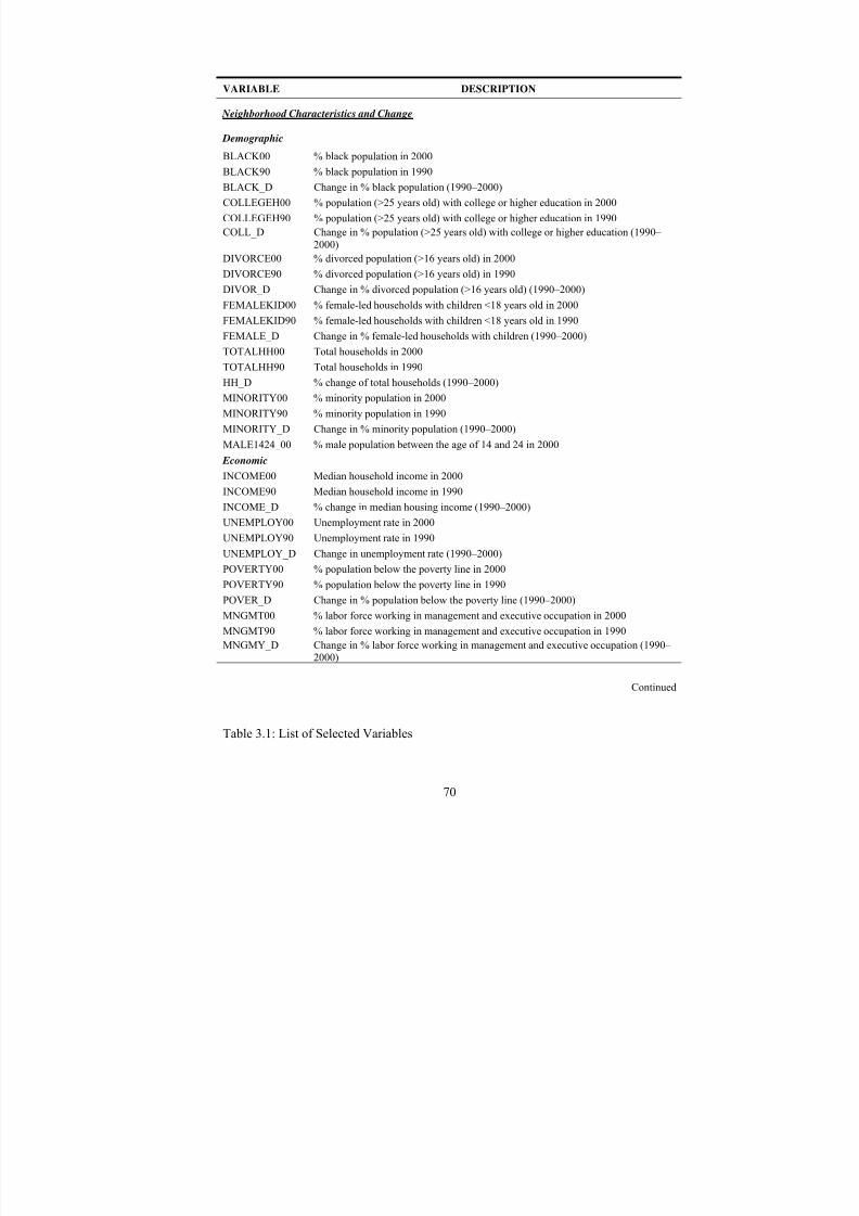
8/6/2019 Spatial Lag Regression
http://slidepdf.com/reader/full/spatial-lag-regression 84/268
70
VARIABLE DESCRIPTION
Neighborhood Characteristics and Change
Demographic
BLACK00 % black population in 2000
BLACK90 % black population in 1990
BLACK_D Change in % black population (1990–2000)
COLLEGEH00 % population (>25 years old) with college or higher education in 2000
COLLEGEH90 % population (>25 years old) with college or higher education in 1990
COLL_D Change in % population (>25 years old) with college or higher education (1990– 2000)
DIVORCE00 % divorced population (>16 years old) in 2000
DIVORCE90 % divorced population (>16 years old) in 1990
DIVOR_D Change in % divorced population (>16 years old) (1990–2000)
FEMALEKID00 % female-led households with children <18 years old in 2000
FEMALEKID90 % female-led households with children <18 years old in 1990
FEMALE_D Change in % female-led households with children (1990–2000)
TOTALHH00 Total households in 2000
TOTALHH90 Total households in 1990
HH_D % change of total households (1990–2000)
MINORITY00 % minority population in 2000
MINORITY90 % minority population in 1990
MINORITY_D Change in % minority population (1990–2000)
MALE1424_00 % male population between the age of 14 and 24 in 2000
Economic
INCOME00 Median household income in 2000
INCOME90 Median household income in 1990INCOME_D % change in median housing income (1990–2000)
UNEMPLOY00 Unemployment rate in 2000
UNEMPLOY90 Unemployment rate in 1990
UNEMPLOY_D Change in unemployment rate (1990–2000)
POVERTY00 % population below the poverty line in 2000
POVERTY90 % population below the poverty line in 1990
POVER_D Change in % population below the poverty line (1990–2000)
MNGMT00 % labor force working in management and executive occupation in 2000
MNGMT90 % labor force working in management and executive occupation in 1990
MNGMY_D Change in % labor force working in management and executive occupation (1990–
2000)
Continued
Table 3.1: List of Selected Variables
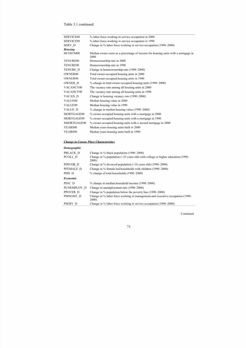
8/6/2019 Spatial Lag Regression
http://slidepdf.com/reader/full/spatial-lag-regression 85/268
71
Table 3.1 continued
SERVICE00 % labor force working in service occupation in 2000
SERVICE90 % labor force working in service occupation in 1990
SERV_D Change in % labor force working in service occupation (1990–2000)
Housing
HCOSTM00 Median owner costs as a percentage of income for housing units with a mortgage in2000
TENURE00 Homeownership rate in 2000
TENURE90 Homeownership rate in 1990
TENURE_D Change in homeownership rate (1990–2000)
OWNER00 Total owner-occupied housing units in 2000
OWNER90 Total owner-occupied housing units in 1990
OWNER_D % change in total owner-occupied housing units (1990–2000)
VACANCY00 The vacancy rate among all housing units in 2000
VACANCY90 The vacancy rate among all housing units in 1990
VACAN_D Change in housing vacancy rate (1990–2000)
VALUE00 Median housing value in 2000
VALUE90 Median housing value in 1990
VALUE_D % change in median housing value (1990–2000)
MORTGAGE00 % owner-occupied housing units with a mortgage in 2000
MORTGAGE90 % owner-occupied housing units with a mortgage in 1990
SMORTGAGE00 % owner-occupied housing units with a second mortgage in 2000
YEARS00 Median years housing units built in 2000
YEARS90 Median years housing units built in 1990
Change in Census Place Characteristics
Demographic
PBLACK_D Change in % black population (1990–2000)
PCOLL_D Change in % population (>25 years old) with college or higher education (1990– 2000)
PDIVOR_D Change in % divorced population (>16 years old) (1990–2000)
PFEMALE_D Change in % female-led households with children (1990–2000)
PHH_D % change of total households (1990–2000)
Economic
PINC_D % change in median household income (1990–2000)
PUNEMPLOY_D Change in unemployment rate (1990–2000)PPOVER_D Change in % population below the poverty line (1990–2000)
PMNGMT_D Change in % labor force working in management and executive occupation (1990– 2000)
PSERV_D Change in % labor force working in service occupation (1990–2000)
Continued

8/6/2019 Spatial Lag Regression
http://slidepdf.com/reader/full/spatial-lag-regression 86/268
8/6/2019 Spatial Lag Regression
http://slidepdf.com/reader/full/spatial-lag-regression 87/268
73
Research Methodology
Simple Descriptive Analysis
After data cleansing, simple descriptive analysis will be used to measure how the
foreclosure cases are distributed over time and place in the two study counties.
Geocoding, geographic aggregation, frequency analysis, univariate analysis, bivariate
analysis, and t-tests will be used in this step of the research.
The geocoding process is the vehicle to find out how those foreclosure cases are
distributed. Each case is geocoded and layered with block groups, the census designated
place, and/or school districts, which provided a convenient way to compare the spatial
pattern in those eight years. All the cases in the eight years are then aggregated at the
block-group level and divided by the total number of owner-occupied housing units in the
same block group to determine a measure of the foreclosure rate. The foreclosure rate
will be classified into five categories and then displayed in a thematic map.
Spatial Analysis
When a variable’s spatial distribution is not random and the values of a variable at a
set of locations depend on values of the same variable at other locations, spatial
autocorrelation exists and will affect the OLS regression results (Odland, 1988). A typical
example in housing market research is housing price. The housing price in a
neighborhood will affect or be affected by the housing price in adjacent neighborhoods.
When we run hedonic housing price models, spatial autocorrelation should be tested. If
the autocorrelation is significant, the spatial lag or error terms should be added to the
hedonic housing price model (Basu and Tribodeau, 1998).
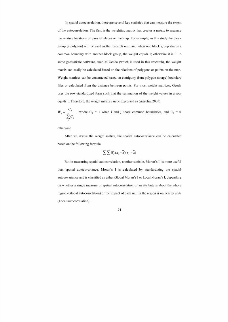
8/6/2019 Spatial Lag Regression
http://slidepdf.com/reader/full/spatial-lag-regression 88/268
8/6/2019 Spatial Lag Regression
http://slidepdf.com/reader/full/spatial-lag-regression 89/268
75
The Global Moran’s I can be expressed as:
∑∑∑
∑∑ −
−−×=
2)(
))((
x x
x x x xW
W
N I
i
jiij
ij
In a row-standardized format of the weighting matrix the term∑∑ ijW
N equals 1.
The Local Moran’s I can be expressed as:
∑= N
j
jijii zW z I
where zi and z j are standardized values of attributes in the region of i and j where
they are neighbors defined according to the weight matrix.
When exploring the spatial autocorrelation of one attribute, univariate Moran’s I is
used, but when exploring the spatial autocorrelation relationship between multiple
variables, for example, to explore whether the foreclosure rate in one neighborhood
would affect the housing price in adjacent neighborhoods, multivariate Moran’s I will be
used.
Spatial Regression
Spatial dependency is a very common phenomenon for geographically distributed
attributes such as those in housing markets. Therefore, when we are dealing with spatial
datasets we initially assume that there is spatial autocorrelation of certain attributes or a
dependency of some attributes on others in neighboring areas. These assumptions make
the research much more complicated, but due to the development of geostatistic
methodology and software incorporating spatial autocorrelation into traditional OLS
regression, the research is feasible.
8/6/2019 Spatial Lag Regression
http://slidepdf.com/reader/full/spatial-lag-regression 90/268
76
The format of a general OLS model can be expressed as:
ξ β += X Y
where Y is the matrix of values for the dependent variable(s), X is the matrix of
values for the independent variables, and ξ is the error-term matrix.
When considering the effect of spatial autocorrelation, the formula can be revised to:
ν ξ ρ β ++= W X Y
where we notice that ρ is the spatial autoregressive coefficient, W is the spatial
weighting matrix, ξ is the spatial error term and υ is another error term. This transformed
OLS regression, which contains a spatial autocorrelation error term, is usually called
spatial error regression.
Another format of spatial regression is based on spatial lags and is called spatial lag
regression. The general format of the spatial lag regression model is:
ν ρ β ++= Wy X Y
where the Wy is a spatially lagged variable of the dependent variable Y
When considering which regression models are appropriate to measure the datasets
(OLS, spatial error, or spatial lag), there are some rules that a researcher can follow,
although these rules are not absolute when making a decision (Anselin, 2005). The
process starts with the Lagrange Multiplier (LM)-error 2 and LM-lag test3. If none of the
tests are significant, then one can choose the OLS model. If only one is significant, then
we should use spatial lag or error models to do further tests. If the LM-error test is
significant, then we should choose the spatial error model; otherwise, we should choose
the spatial lag model.
8/6/2019 Spatial Lag Regression
http://slidepdf.com/reader/full/spatial-lag-regression 91/268
77
If both the LM-error and LM-lag tests are significant, then we look at the Robust
LM-error diagnostic. If the Robust LM-error 4 is significant, we choose the spatial error
model, and if the Robust LM-lag is significant, we choose the spatial lag model. See
Figure 3.1 for a summary of this process.
In this research, when measuring neighborhood effects on foreclosures the OLS
model will be tested in both counties. If the effect is different in each county, then the
analysis will run the OLS models separately for the counties. If the OLS spatial
dependence diagnosis finds significant spatial dependence spatial error or lag models will
be used to estimate the neighborhood effects. The rule of choosing between the error or
lag models is based on the chart in Figure 3.1.
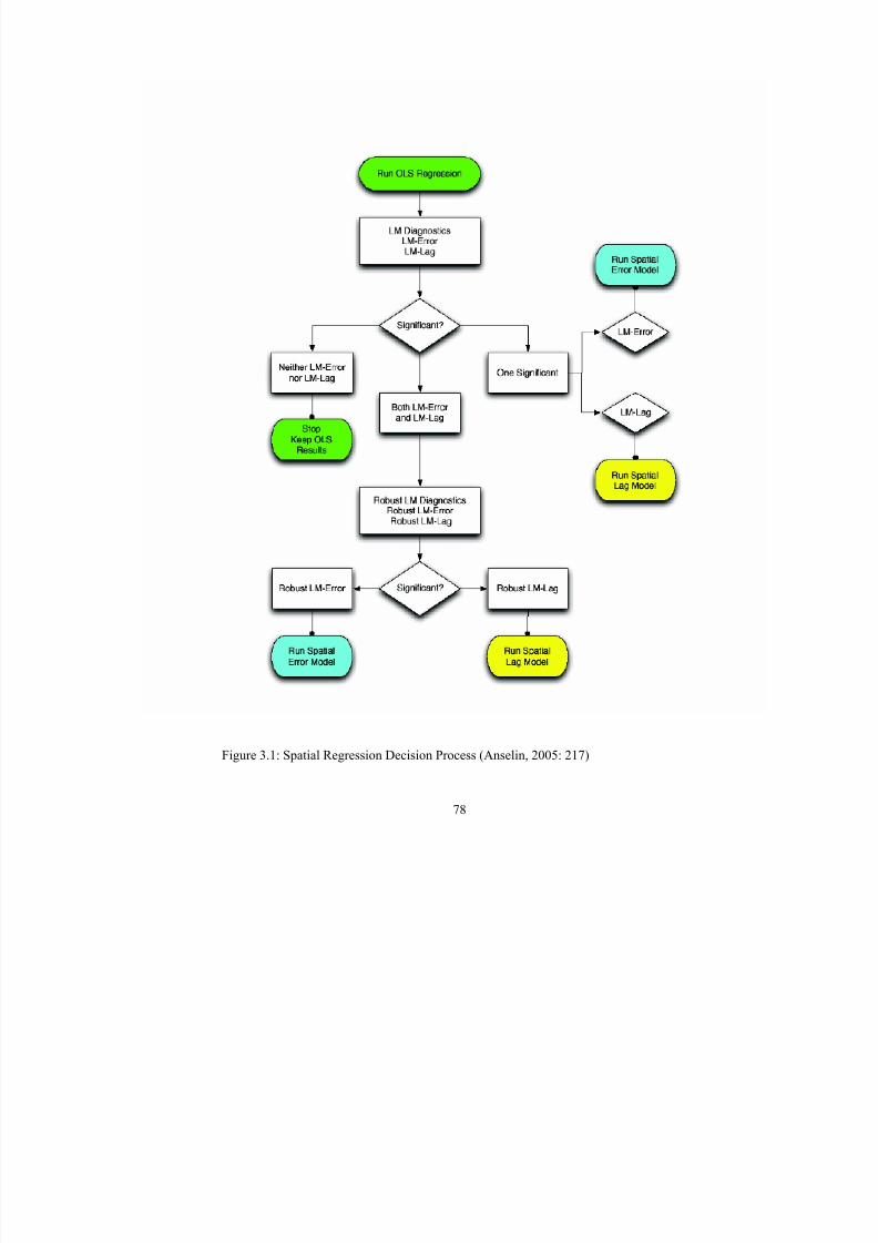
8/6/2019 Spatial Lag Regression
http://slidepdf.com/reader/full/spatial-lag-regression 92/268
78
Figure 3.1: Spatial Regression Decision Process (Anselin, 2005: 217)
8/6/2019 Spatial Lag Regression
http://slidepdf.com/reader/full/spatial-lag-regression 93/268
79
Seemingly Unrelated Regression (SUR)
Seemingly unrelated regression (SUR), also called joint generalized least squares
(JGLS) or Zellner estimation, is a system of OLS for multiple equations. Like OLS, SUR
assumes that all the regressors are independent variables, but SUR uses the correlations
among the errors in different equations to improve the regression estimates. The SUR
method requires an initial OLS regression to compute residuals. The OLS residuals are
used to estimate the cross-equation covariance matrix.
SUR may improve the efficiency of parameter estimates when there is
contemporaneous correlation of errors across equations. Under two sets of circumstances,
SUR parameter estimates are the same as those produced by OLS: when there is no
contemporaneous correlation of errors across equations (the estimate of contemporaneous
correlation matrix is diagonal); and when the independent variables are the same across
equations.
Theoretically, SUR parameter estimates will always be at least as efficient as OLS
in large samples, provided that the equations are correctly specified. However, in small
samples the need to estimate the covariance matrix from the OLS residuals increases the
sampling variability of the SUR estimates, and this effect can cause SUR to be less
efficient than OLS. If the sample size is small and the across-model correlations are
small, then OLS is preferred to SUR. The consequences of specification error are also
more serious with SUR than with OLS.
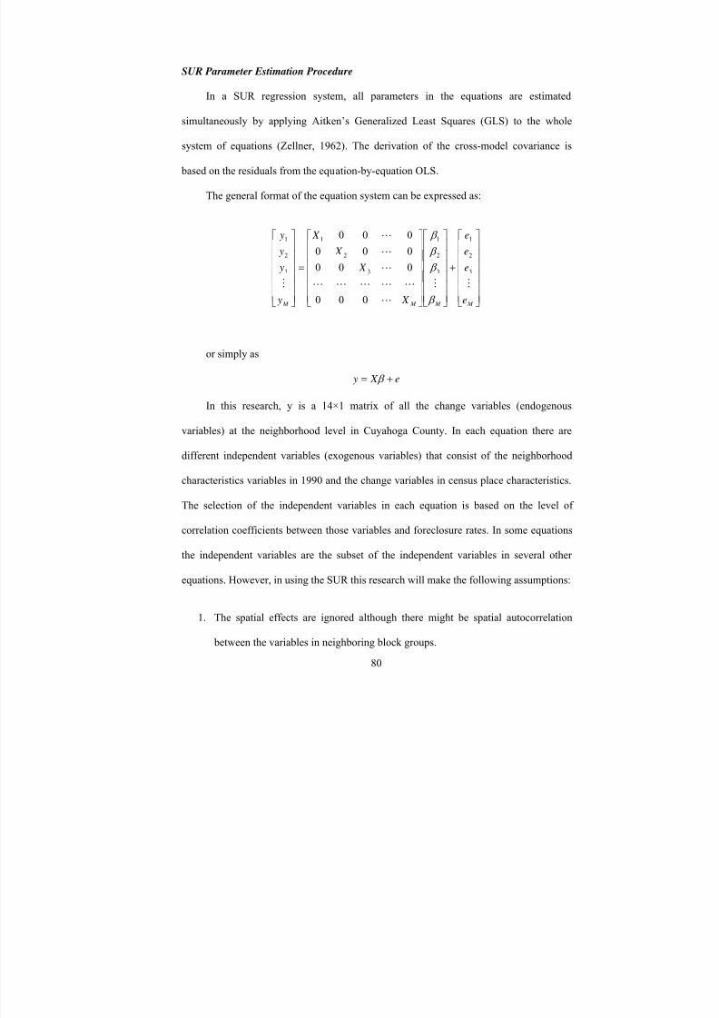
8/6/2019 Spatial Lag Regression
http://slidepdf.com/reader/full/spatial-lag-regression 94/268
80
SUR Parameter Estimation Procedure
In a SUR regression system, all parameters in the equations are estimated
simultaneously by applying Aitken’s Generalized Least Squares (GLS) to the whole
system of equations (Zellner, 1962). The derivation of the cross-model covariance is
based on the residuals from the equation-by-equation OLS.
The general format of the equation system can be expressed as:
⎥⎥⎥⎥⎥⎥
⎦
⎤
⎢⎢⎢⎢⎢⎢
⎣
⎡
+
⎥⎥⎥⎥⎥⎥
⎦
⎤
⎢⎢⎢⎢⎢⎢
⎣
⎡
⎥⎥⎥⎥⎥⎥
⎦
⎤
⎢⎢⎢⎢⎢⎢
⎣
⎡
=
⎥⎥⎥⎥⎥⎥
⎦
⎤
⎢⎢⎢⎢⎢⎢
⎣
⎡
M M M M e
e
e
e
X
X
X
X
y
y
y
y
MM
L
LLLLL
L
L
L
M
3
2
1
3
2
1
3
2
1
3
2
1
000
000
000
000
β
β
β
β
or simply as
e X y += β
In this research, y is a 14×1 matrix of all the change variables (endogenous
variables) at the neighborhood level in Cuyahoga County. In each equation there are
different independent variables (exogenous variables) that consist of the neighborhood
characteristics variables in 1990 and the change variables in census place characteristics.
The selection of the independent variables in each equation is based on the level of
correlation coefficients between those variables and foreclosure rates. In some equations
the independent variables are the subset of the independent variables in several other
equations. However, in using the SUR this research will make the following assumptions:
1. The spatial effects are ignored although there might be spatial autocorrelation
between the variables in neighboring block groups.
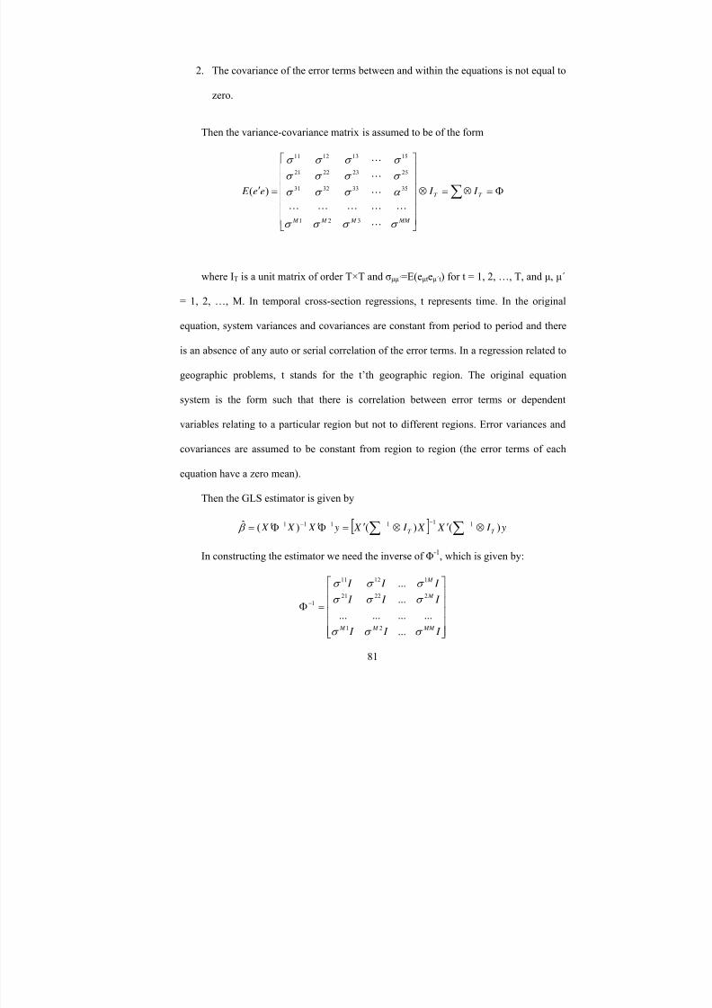
8/6/2019 Spatial Lag Regression
http://slidepdf.com/reader/full/spatial-lag-regression 95/268
81
2. The covariance of the error terms between and within the equations is not equal to
zero.
Then the variance-covariance matrix is assumed to be of the form
∑ Φ=⊗=⊗
⎥⎥⎥⎥⎥⎥
⎦
⎤
⎢⎢⎢⎢⎢⎢
⎣
⎡
=′T T
MM M M M
I I ee E
σ σ σ σ
α σ σ σ
σ σ σ σ
σ σ σ σ
L
LLLLL
L
L
L
321
35333231
25232221
15131211
)(
where IT is a unit matrix of order T×T and σμμ΄=E(eμteμ΄t) for t = 1, 2, …, T, and μ, μ΄
= 1, 2, …, M. In temporal cross-section regressions, t represents time. In the original
equation, system variances and covariances are constant from period to period and there
is an absence of any auto or serial correlation of the error terms. In a regression related to
geographic problems, t stands for the t’th geographic region. The original equation
system is the form such that there is correlation between error terms or dependent
variables relating to a particular region but not to different regions. Error variances and
covariances are assumed to be constant from region to region (the error terms of each
equation have a zero mean).
Then the GLS estimator is given by
[ ] y I X X I X y X X X T T )()()(ˆ 111111 ⊗′⊗′=Φ′Φ′= ∑∑ −−−−−− β
In constructing the estimator we need the inverse of Φ-1
, which is given by:
⎥⎥⎥⎥⎥
⎦
⎤
⎢⎢⎢⎢⎢
⎣
⎡
=Φ −
I I I
I I I
I I I
MM M M
M
M
σ σ σ
σ σ σ
σ σ σ
...
............
...
...
21
22221
11211
1
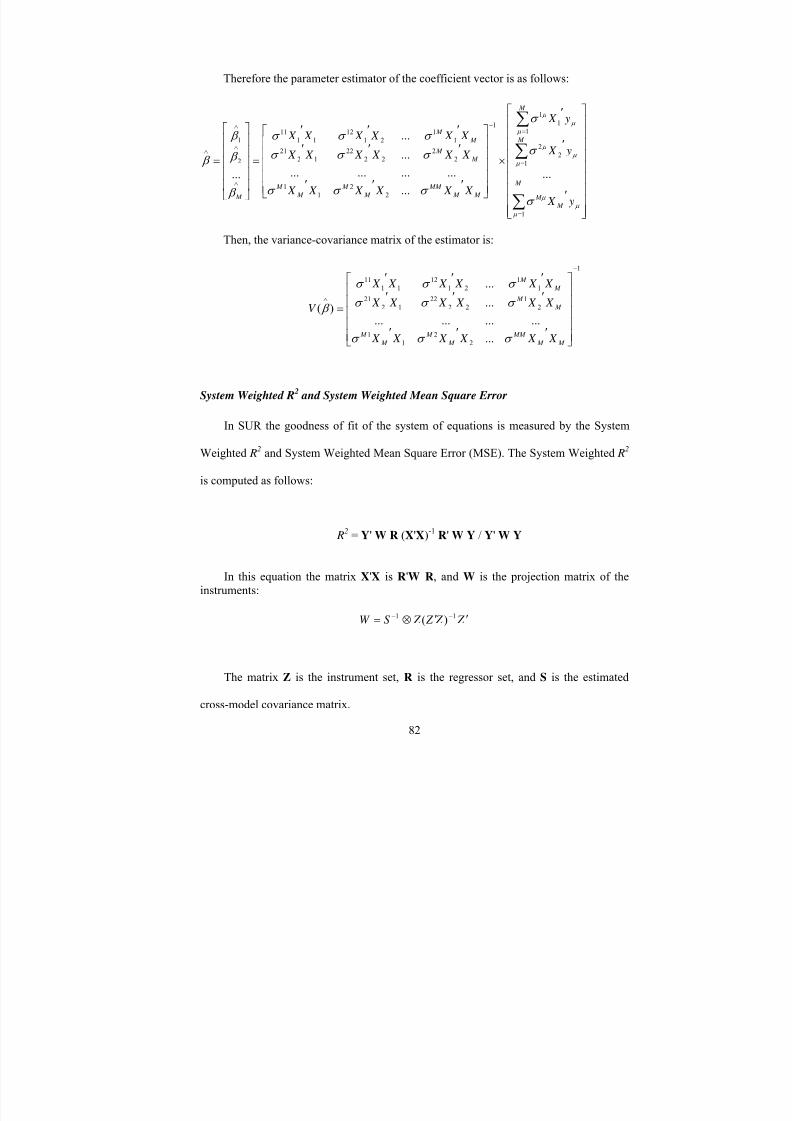
8/6/2019 Spatial Lag Regression
http://slidepdf.com/reader/full/spatial-lag-regression 96/268
82
Therefore the parameter estimator of the coefficient vector is as follows:
⎥⎥⎥⎥⎥⎥⎥
⎥⎥
⎦
⎤
⎢⎢⎢⎢⎢⎢⎢
⎢⎢
⎣
⎡
′
′
′
×
⎥⎥⎥⎥⎥
⎦
⎤
⎢⎢⎢⎢⎢
⎣
⎡
′′′
′′′
′′′
=
⎥⎥⎥⎥
⎥
⎦
⎤
⎢⎢⎢⎢
⎢
⎣
⎡
=
∑
∑
∑
=
=
=−
∧
∧
∧
∧
M
M
M
M
M
M M
MM
M
M
M
M
M M
M
M
M y X
y X
y X
X X X X X X
X X X X X X
X X X X X X
1
1
2
2
1
1
1
1
2
2
1
1
22
2222
1221
11
2112
1111
2
1
...
...
............
...
...
...
μ
μ
μ
μ
μ
μ
μ
μ
μ
σ
σ
σ
σ σ σ
σ σ σ
σ σ σ
β
β
β
β
Then, the variance-covariance matrix of the estimator is:
System Weighted R 2
and System Weighted Mean Square Error
In SUR the goodness of fit of the system of equations is measured by the System
Weighted R2
and System Weighted Mean Square Error (MSE). The System Weighted R2
is computed as follows:
R2 = Y' W R (X'X)-1 R' W Y / Y' W Y
In this equation the matrix X'X is R'W R, and W is the projection matrix of theinstruments:
Z Z Z Z SW ′′⊗= −− 11 )(
The matrix Z is the instrument set, R is the regressor set, and S is the estimated
cross-model covariance matrix.
1
2
2
1
1
2
1
22
22
12
21
1
1
21
12
11
11
...
...............
...
)(
−
∧
⎥⎥⎥⎥
⎥
⎦
⎤
⎢⎢⎢⎢
⎢
⎣
⎡
′′′
′′′
′′′
=
M M
MM
M
M
M
M
M
M
M
M
X X X X X X
X X X X X X
X X X X X X
V
σ σ σ
σ σ σ
σ σ σ
β

8/6/2019 Spatial Lag Regression
http://slidepdf.com/reader/full/spatial-lag-regression 97/268
83
The system weighted MSE is computed as follows:
MSE = [1/tdf ] ( Y' W Y - Y' W R (X'X)-1
R' W Y )
In this equation, tdf is the sum of the error degrees of freedom for the equations in
the system.
8/6/2019 Spatial Lag Regression
http://slidepdf.com/reader/full/spatial-lag-regression 98/268
84
CHAPTER 4
DESCRIPTIVE AND SPATIAL ANALYSIS
Judicial Foreclosure Process and Sheriff’s Deed Transfer Data
When borrowers are in default, usually defined as being three months behind in
mortgage repayments, lenders in some states can file a foreclosure lawsuit in the local
civic court and initiate a judicial foreclosure process. In other states, lenders file a notice
of default and initiate a trustee’s sale of the properties without going through the judicial
system. This is called non-judicial foreclosure. In some states both judicial and non-
judicial systems exist. In Ohio, only judicial foreclosure is allowed.
There are several critical procedures in the process of judicial foreclosure. When the
mortgage lender detects a loan default, they will notify the loan borrower about the
default and possible plans to restore a normal status. If the borrower does not respond, or
the work-out plans or loan modification plans fail, the lender will file a civil lawsuit
against the borrower (mortgagor) to claim the payoff of the loan balance. This is the start
of the foreclosure process. If at this stage the borrower repays the loan, sells the property
and pays off the loan, or files for bankruptcy the case will be finalized. If none of these
occur, the property, as collateral for the mortgage, will be put into a civic sale. These
sales are usually conducted by the Sheriff’s Office of each county, which holds an
8/6/2019 Spatial Lag Regression
http://slidepdf.com/reader/full/spatial-lag-regression 99/268
85
auction on a regular basis. If the loan balance is fully paid, or the borrower announces
bankruptcy, or the property is bought by private investors prior the auction, the property
will be withdrawn from the sales process. Otherwise, the property will go to the Sheriff’s
Sale. If no bid is made on a property the lenders will usually take the title of the property
to sell in the future; this kind of property is called a Real Estate Owned (REO) property.
Properties sold at the Sheriff’s sales will be recorded at the county Recorders’ Office as
Sheriff’s Deeds. The process of judicial foreclosure and the handling of the properties
before and after foreclosure is summarized in Figure 4.1.
Because of the complex nature of the process when conducting foreclosure
research, it is difficult to decide what datasets to use. The choice largely depends on the
objectives of the research. If we want to know what factors lead to foreclosures,
foreclosure filing datasets or mortgage loan performance datasets can be used. But if we
want to explore the impact of the foreclosure process (from foreclosure start to finish) on
neighborhood characteristics and change, it is appropriate to use the Sheriff’s Deeds
transfer data since those properties are foreclosed and probably have the biggest impact
on neighborhoods.
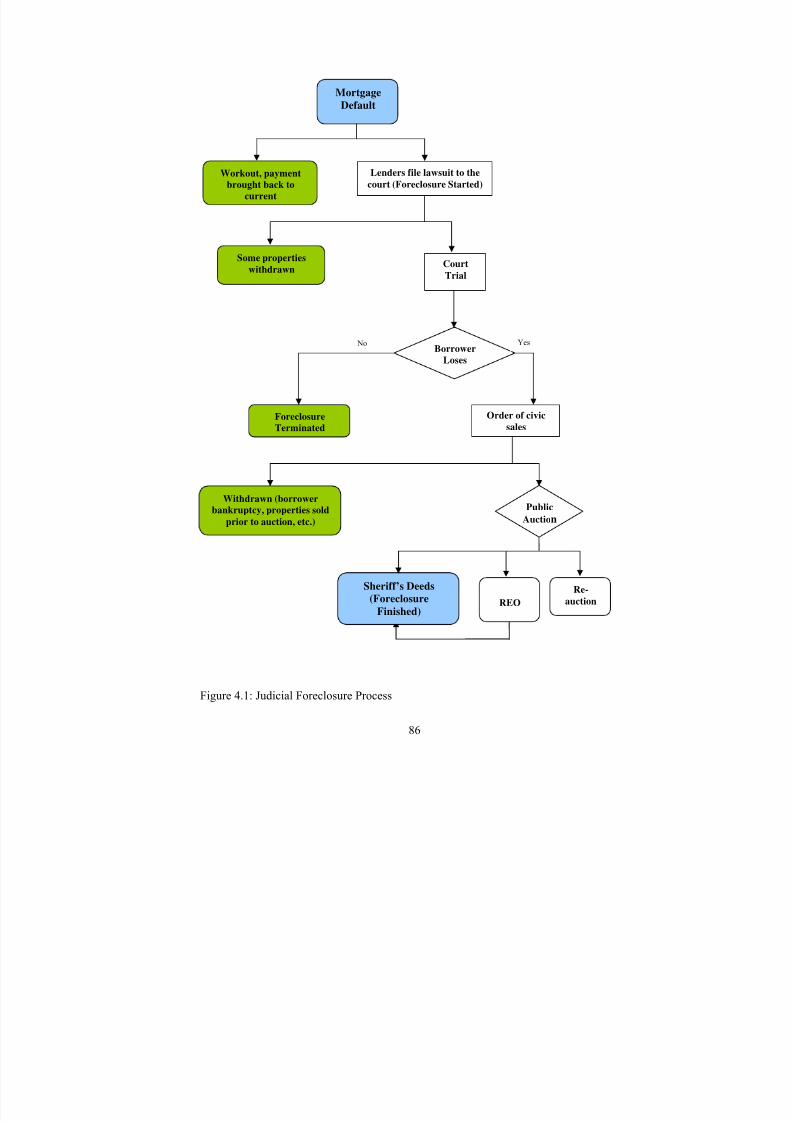
8/6/2019 Spatial Lag Regression
http://slidepdf.com/reader/full/spatial-lag-regression 100/268
86
Figure 4.1: Judicial Foreclosure Process
Lenders file lawsuit to the
court (Foreclosure Started)
Court
Trial
Borrower
Loses
Order of civic
sales
Public
Auction
Sheriff’s Deeds
(Foreclosure
Finished)
Re-
auction
Mortgage
Default
Workout, payment
brought back to
current
Some properties
withdrawn
Foreclosure
Terminated
Withdrawn (borrower
bankruptcy, properties sold
prior to auction, etc.)
REO
No Yes
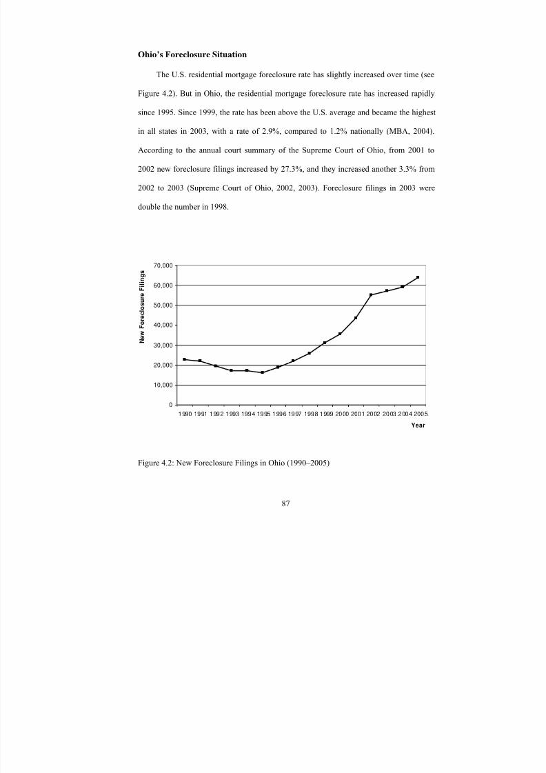
8/6/2019 Spatial Lag Regression
http://slidepdf.com/reader/full/spatial-lag-regression 101/268
87
Ohio’s Foreclosure Situation
The U.S. residential mortgage foreclosure rate has slightly increased over time (see
Figure 4.2). But in Ohio, the residential mortgage foreclosure rate has increased rapidly
since 1995. Since 1999, the rate has been above the U.S. average and became the highest
in all states in 2003, with a rate of 2.9%, compared to 1.2% nationally (MBA, 2004).
According to the annual court summary of the Supreme Court of Ohio, from 2001 to
2002 new foreclosure filings increased by 27.3%, and they increased another 3.3% from
2002 to 2003 (Supreme Court of Ohio, 2002, 2003). Foreclosure filings in 2003 were
double the number in 1998.
Figure 4.2: New Foreclosure Filings in Ohio (1990–2005)
0
10,000
20,000
30,000
40,000
50,000
60,000
70,000
1990 1991 1992 1993 1994 1995 1996 1997 1998 1999 2000 2001 2002 2003 2004 2005
Year
N e w
F o r e c
l o s u r e F i l i n g s
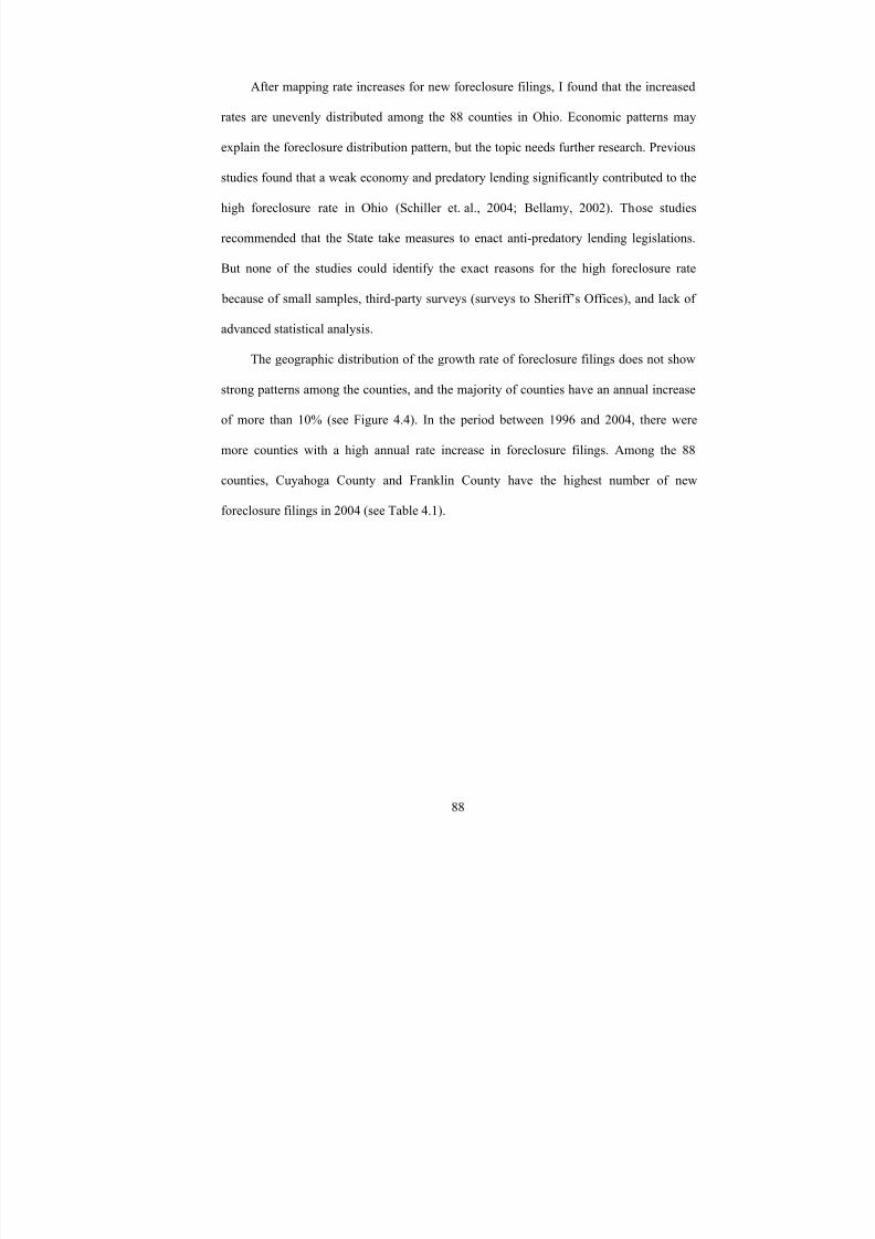
8/6/2019 Spatial Lag Regression
http://slidepdf.com/reader/full/spatial-lag-regression 102/268
88
After mapping rate increases for new foreclosure filings, I found that the increased
rates are unevenly distributed among the 88 counties in Ohio. Economic patterns may
explain the foreclosure distribution pattern, but the topic needs further research. Previous
studies found that a weak economy and predatory lending significantly contributed to the
high foreclosure rate in Ohio (Schiller et. al., 2004; Bellamy, 2002). Those studies
recommended that the State take measures to enact anti-predatory lending legislations.
But none of the studies could identify the exact reasons for the high foreclosure rate
because of small samples, third-party surveys (surveys to Sheriff’s Offices), and lack of
advanced statistical analysis.
The geographic distribution of the growth rate of foreclosure filings does not show
strong patterns among the counties, and the majority of counties have an annual increase
of more than 10% (see Figure 4.4). In the period between 1996 and 2004, there were
more counties with a high annual rate increase in foreclosure filings. Among the 88
counties, Cuyahoga County and Franklin County have the highest number of new
foreclosure filings in 2004 (see Table 4.1).
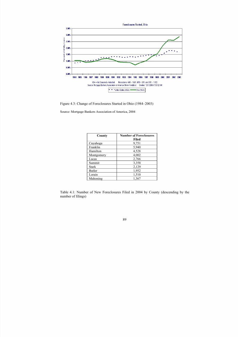
8/6/2019 Spatial Lag Regression
http://slidepdf.com/reader/full/spatial-lag-regression 103/268
89
Figure 4.3: Change of Foreclosures Started in Ohio (1984–2003)
Source: Mortgage Bankers Association of America, 2004
Table 4.1: Number of New Foreclosures Filed in 2004 by County (descending by thenumber of filings)
County Number of ForeclosuresFiled
Cuyahoga 9,751
Franklin 5,940
Hamilton 4,528
Montgomery 4,002
Lucas 2,766
Summit 3,358
Stark 2,129
Butler 1,952
Lorain 1,510
Mahoning 1,367
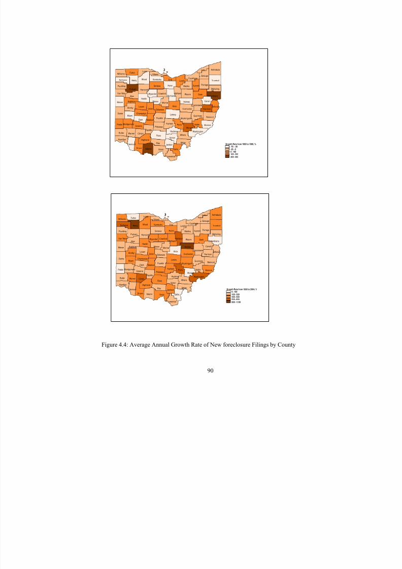
8/6/2019 Spatial Lag Regression
http://slidepdf.com/reader/full/spatial-lag-regression 104/268
90
Ross
Stark
Wood
Knox
Darke
Pike
Licking
Scioto
Allen
Adams
Huron
Lorain
Gallia
Wayne
Butler
Brown
Perry
Clark
LoganUnion
Trumbull
Seneca
Ashtabula
Athens
Henry
Hardin
Erie
Meigs
Noble
Miami
Mercer
Franklin
Fulton
Belmont
Portage
Preble
Vinton
Putnam
Fairfield
Highland
Hancock
Carroll
Shelby
Monroe
Lucas
Marion
Medina
Muskingum
Clinton
Richland
Holmes
Summit
GreeneMorgan
Morrow
Madison
Guernsey
Fayette
Warren
Pickaway
Ashland
Coshocton
Washington
Geauga
Hocking
Williams
JacksonClermont
Lake
Paulding
HarrisonDelaware
Tuscarawas
Defiance
Auglaize
Lawrence
Cuyahoga
Wyandot
Hamilton
ColumbianaCrawford
Jefferson
Mahoning
Van Wert
Sandusky
Ottawa
Champaign
Montgomery
Growth Rate from 1996 to 2004, %0 - 100
100 - 300300 - 500500 - 800
800 - 1100
Ross
Stark
Wood
Knox
Darke
Pike
Licking
Scioto
Allen
Adams
Huron
Lorain
Gallia
Wayne
Butler
Brown
Perry
Clark
LoganUnion
Trumbull
Seneca
Ashtabula
Athens
Henry
Hardin
Erie
Meigs
Noble
Miami
Mercer
Franklin
Fulton
Belmont
Portage
Preble
Vinton
Putnam
Fairfield
Highland
Hancock
Carroll
Shelby
Monroe
Lucas
Marion
Medina
Muskingum
Clinton
Richland
Holmes
Summit
GreeneMorgan
Morrow
Madison
Guernsey
Fayette
Warren
Pickaway
Ashland
Coshocton
Washington
Geauga
Hocking
Williams
JacksonClermont
Lake
Paulding
HarrisonDelaware
Tuscarawas
Defiance
Auglaize
Lawrence
Cuyahoga
Wyandot
Hamilton
ColumbianaCrawford
Jefferson
Mahoning
Van Wert
Sandusky
Ottawa
Champaign
Montgomery
Growth Rate from 1990 to 1996, %-70 - -35
-35 - 00 - 100
100 - 200200 - 360
Figure 4.4: Average Annual Growth Rate of New foreclosure Filings by County
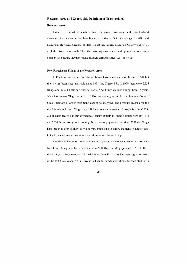
8/6/2019 Spatial Lag Regression
http://slidepdf.com/reader/full/spatial-lag-regression 105/268
91
Research Area and Geographic Definition of Neighborhood
Research Area
Initially, I hoped to explore how mortgage foreclosure and neighborhood
characteristics interact in the three biggest counties in Ohio: Cuyahoga, Franklin and
Hamilton. However, because of data availability issues, Hamilton County had to be
excluded from the research. The other two major counties should provide a good study
comparison because they have quite different characteristics (see Table 4.2).
New Foreclosure Filings of the Research Area
In Franklin County new foreclosure filings have risen continuously since 1990, but
the rise has been steep and rapid since 1995 (see Figure 4.5). In 1990 there were 2,533
filings and by 2004 this had risen to 5,940. New filings doubled during those 15 years.
New foreclosure filing data prior to 1990 was not aggregated by the Supreme Court of
Ohio, therefore a longer term trend cannot be analyzed. The potential reasons for the
rapid increases in new filings since 1995 are not clearly known, although Schiller (2003,
2004) stated that the unemployment rate cannot explain the trend because between 1995
and 2000 the economy was booming. It is encouraging to see that since 2002 the filings
have begun to drop slightly. It will be very interesting to follow the trend in future years
to try to connect macro economic trends to new foreclosure filings.
Foreclosure has been a serious issue in Cuyahoga County since 1990. In 1990 new
foreclosure filings numbered 5,595, and in 2004 the new filings jumped to 9,751. Over
those 15 years there were 84,672 total filings. Franklin County has seen slight decreases
in the last three years, but in Cuyahoga County foreclosure filings dropped slightly in
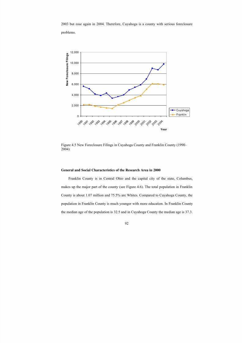
8/6/2019 Spatial Lag Regression
http://slidepdf.com/reader/full/spatial-lag-regression 106/268
92
2003 but rose again in 2004. Therefore, Cuyahoga is a county with serious foreclosure
problems.
0
2,000
4,000
6,000
8,000
10,000
12,000
1 9 9 0
1 9 9 1
1 9 9 2
1 9 9 3
1 9 9 4
1 9 9 5
1 9 9 6
1 9 9 7
1 9 9 8
1 9 9 9
2 0 0 0
2 0 0 1
2 0 0 2
2 0 0 3
2 0 0 4
Year
N e w
F o r e c l o s u r e F i l i n g s
Cuyahoga
Franklin
Figure 4.5 New Foreclosure Filings in Cuyahoga County and Franklin County (1990– 2004)
General and Social Characteristics of the Research Area in 2000
Franklin County is in Central Ohio and the capital city of the state, Columbus,
makes up the major part of the county (see Figure 4.6). The total population in Franklin
County is about 1.07 million and 75.5% are Whites. Compared to Cuyahoga County, the
population in Franklin County is much younger with more education. In Franklin County
the median age of the population is 32.5 and in Cuyahoga County the median age is 37.3.

8/6/2019 Spatial Lag Regression
http://slidepdf.com/reader/full/spatial-lag-regression 107/268
93
In Franklin County 85.7% of the population are high school graduates (or higher),
compared to 81.6% in Cuyahoga County.
Cuyahoga County is located at the northeastern corner of the state and Cleveland
makes up the major part of the county (see Figure 4.6). The total population in Cuyahoga
County is 1.39 million and 67.4% are Whites. Therefore, Cuyahoga County has a larger
percentage of a minority population.
There are 438,778 total housing units in Franklin County and 56.9% are owner-
occupied. Female headship rate, defined as the percentage of female householders
without a husband present, is 13.0%.
There are 616,903 total housing units in Cuyahoga County and 63.2% are owner-
occupied. Female headship rate is 15.7%.
Economic Characteristics of the Research Area
In Franklin County 70.7% of the population over 16 are in the labor force, and in
Cuyahoga County the ratio is 62.5%. In 2000 the unemployment rate was 3.0% in
Franklin County and 3.9% in Cuyahoga County. The 2005 unemployment rate was 6.1%
for Cuyahoga County and 5.3% for Franklin County. This increase in unemployment may
have contributed to overall increases in foreclosures.
Median household income in Franklin County is $42,734 (in 2004 inflation-adjusted
dollars); in Cuyahoga County it is $39,168. And, in Franklin County there are fewer
families that are under the poverty line (8.2%, compared to 10.2% in Cuyahoga County).
Generally speaking, the economic situation in Franklin County is better than that in
Cuyahoga County with a higher household income, lower poverty rate, and a lower
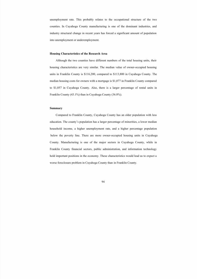
8/6/2019 Spatial Lag Regression
http://slidepdf.com/reader/full/spatial-lag-regression 108/268
94
unemployment rate. This probably relates to the occupational structure of the two
counties. In Cuyahoga County manufacturing is one of the dominant industries, and
industry structural change in recent years has forced a significant amount of population
into unemployment or underemployment.
Housing Characteristics of the Research Area
Although the two counties have different numbers of the total housing units, their
housing characteristics are very similar. The median value of owner-occupied housing
units in Franklin County is $116,200, compared to $113,800 in Cuyahoga County. The
median housing costs for owners with a mortgage is $1,077 in Franklin County compared
to $1,057 in Cuyahoga County. Also, there is a larger percentage of rental units in
Franklin County (43.1%) than in Cuyahoga County (36.8%).
Summary
Compared to Franklin County, Cuyahoga County has an older population with less
education. The county’s population has a larger percentage of minorities, a lower median
household income, a higher unemployment rate, and a higher percentage population
below the poverty line. There are more owner-occupied housing units in Cuyahoga
County. Manufacturing is one of the major sectors in Cuyahoga County, while in
Franklin County financial sectors, public administration, and information technology
hold important positions in the economy. These characteristics would lead us to expect a
worse foreclosure problem in Cuyahoga County than in Franklin County.
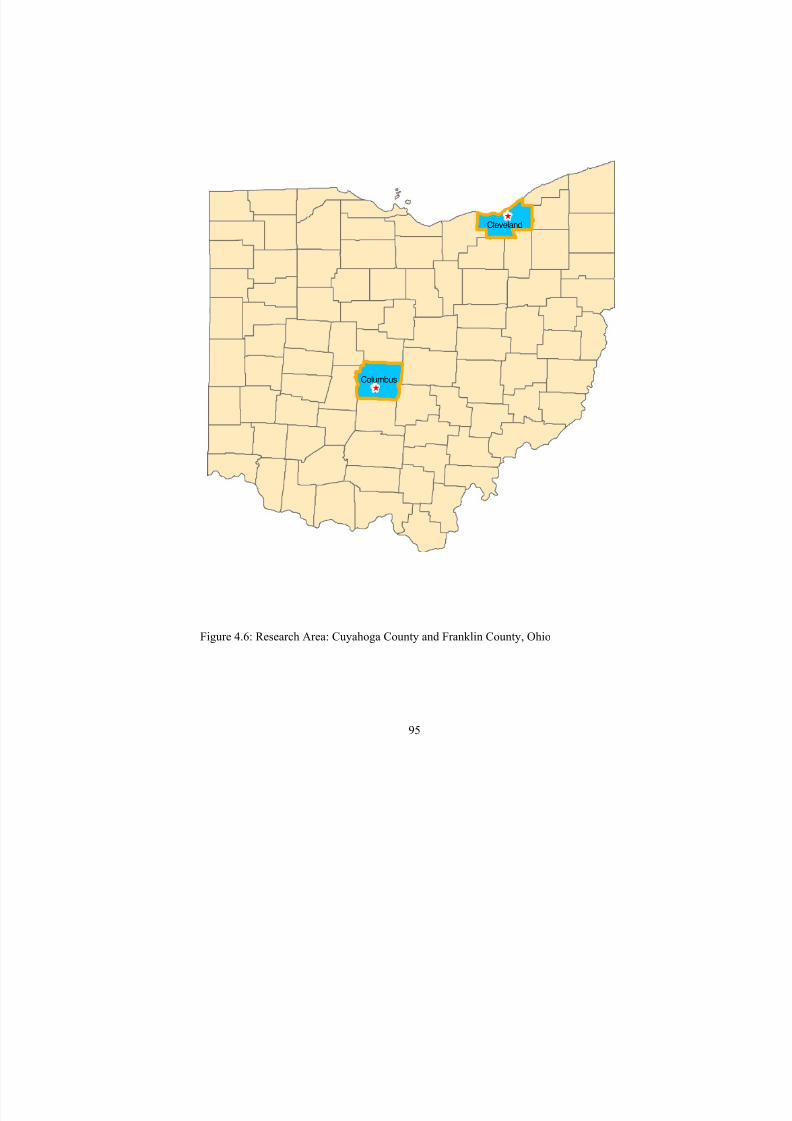
8/6/2019 Spatial Lag Regression
http://slidepdf.com/reader/full/spatial-lag-regression 109/268
95
Columbus
Cleveland[
[
Figure 4.6: Research Area: Cuyahoga County and Franklin County, Ohio

8/6/2019 Spatial Lag Regression
http://slidepdf.com/reader/full/spatial-lag-regression 110/268
96
2000
Franklin County Cuyahoga County
Number % Number %
General Characteristics
Total population 1,068,978 - 1,393,978 -
Median age (years) 32.5 - 37.3 -
White 806,851 75.50 938,863 67.40
Black or African American 191,196 17.90 382,634 27.40
American Indian and Alaska Native 2,899 0.30 2,529 0.20
Asian 32,784 3.10 25,245 1.80
Native Hawaiian and Other Pacific Islander 466 0.00 338 0.00
Some other race 10,992 1.00 20,962 1.50
Two or more races 23,790 2.20 23,407 1.70
Average household size 2.39 - 2.39 -
Female householder, no husband present 57,195 13.00 89,793 15.70
With own children under 18 years old 36,260 8.30 51,100 8.90
Average family size 3.03 - 3.06 -
Total housing units 438,778 93.20 616,903 -
Owner-occupied housing units 249,633 56.90 360,980 63.20
Renter-occupied housing units 189,145 43.10 210,477 36.80
Vacant housing units 32,238 6.80 45,446 7.40
Social Characteristics
High school graduate or higher 579,896 85.70 764,186 81.60
Bachelor's degree or higher 215,180 31.80 235,413 25.10
Male, Now married, except separated (>= 15 years old) 201,802 50.10 261,433 51.40Female, Now married, except separated (>=15 yearsold) 201,354 45.90 261,741 44.10
Economic Characteristics
In labor force (>= 16 years old) 584,391 70.70 676,874 62.50
Unemployed 24,594 3.00 41,778 3.90
Median household income (in 2004 inflation-adjusteddollars) 42,734 - 39,168 -
Median family income (in 2004 inflation-adjusteddollars) 53,905 - 49,559 -
Per capita income (in 2004 inflation-adjusted dollars) 23,059 - 22,272 -
Families below poverty level 21,742 8.20 36,535 10.30
Female householder, no husband present 13,787 24.30 - -Female householder, no husband present, with
children < 18 12,421 30.30 - -
Individuals below poverty level 121,843 11.60 179,372 13.10
Continued
Table 4.2: Selected Characteristics of the Two Counties
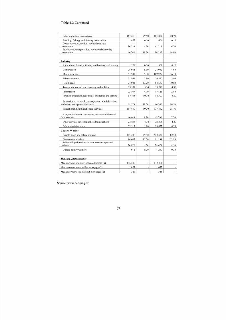
8/6/2019 Spatial Lag Regression
http://slidepdf.com/reader/full/spatial-lag-regression 111/268
97
Table 4.2 Continued
Sales and office occupations 167,418 29.90 181,884 28.70
Farming, fishing, and forestry occupations 472 0.10 606 0.10
Construction, extraction, and maintenanceoccupations 36,533 6.50 42,211 6.70
Production, transportation, and material-movingoccupations 66,742 11.90 94,237 14.90
Industry
Agriculture, forestry, fishing and hunting, and mining 1,229 0.20 901 0.10
Construction 28,664 5.10 28,952 4.60
Manufacturing 51,907 9.30 102,279 16.10
Wholesale trade 21,861 3.90 24,570 3.90
Retail trade 74,001 13.20 68,699 10.80
Transportation and warehousing, and utilities 29,537 5.30 30,779 4.90
Information 22,167 4.00 17,821 2.80
Finance, insurance, real estate, and rental and leasing 57,468 10.30 54,773 8.60
Professional, scientific, management, administrative,and waste management services 61,573 11.00 64,340 10.10
Educational, health and social services 107,669 19.30 137,562 21.70
Arts, entertainment, recreation, accommodation andfood services 46,648 8.30 48,796 7.70
Other services (except public administration) 23,888 4.30 28,090 4.40
Public administration 32,517 5.80 26,857 4.20
Class of Worker
Private wage and salary workers 445,498 79.70 523,380 82.50
Government workers 86,647 15.50 81,138 12.80
Self-employed workers in own non-incorporated business 26,072 4.70 28,671 4.50
Unpaid family workers 912 0.20 1,230 0.20
Housing Characteristics
Median value of owner-occupied homes ($) 116,200 - 113,800 -
Median owner costs with a mortgage ($) 1,077 - 1,057 -
Median owner costs without mortgages ($) 326 - 346 -
Source: www.census.gov

8/6/2019 Spatial Lag Regression
http://slidepdf.com/reader/full/spatial-lag-regression 112/268
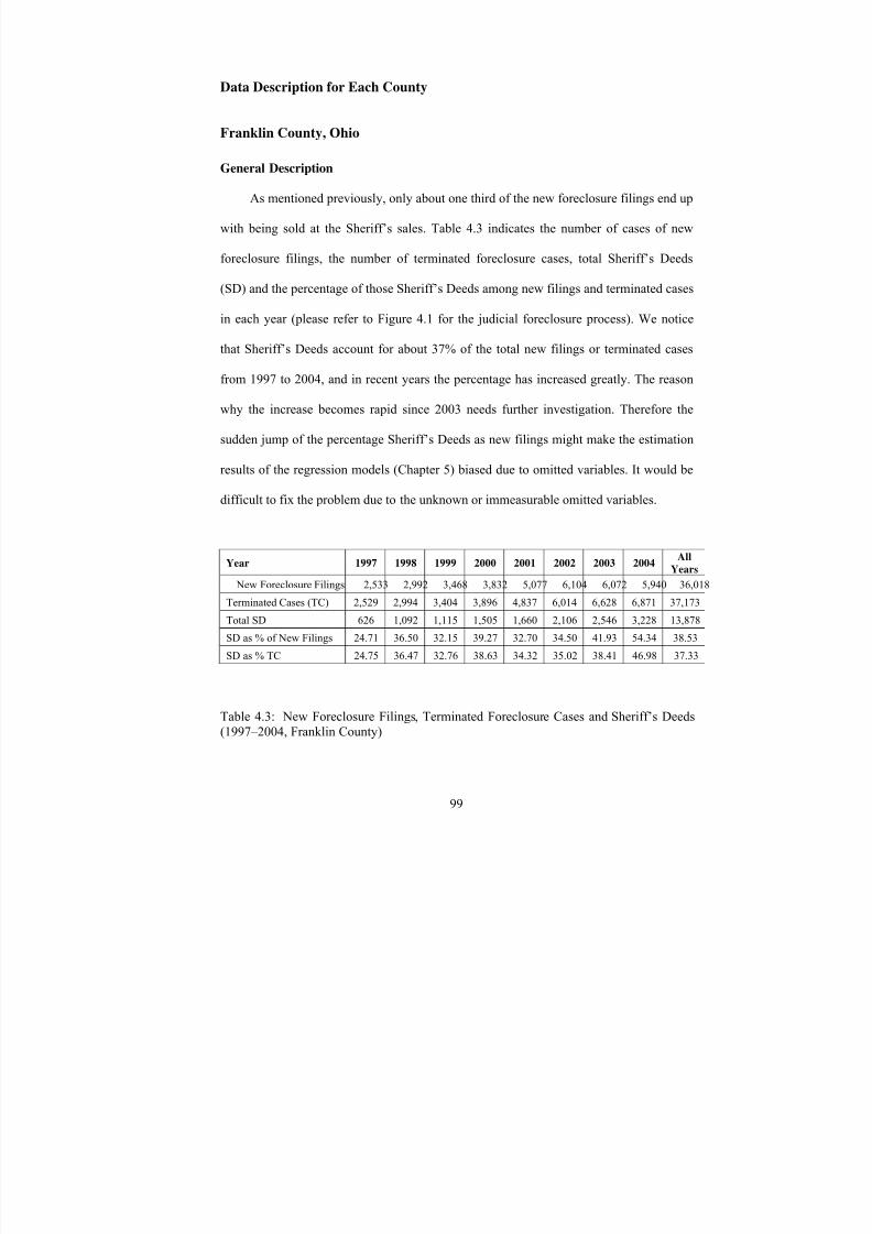
8/6/2019 Spatial Lag Regression
http://slidepdf.com/reader/full/spatial-lag-regression 113/268
99
Data Description for Each County
Franklin County, Ohio
General Description
As mentioned previously, only about one third of the new foreclosure filings end up
with being sold at the Sheriff’s sales. Table 4.3 indicates the number of cases of new
foreclosure filings, the number of terminated foreclosure cases, total Sheriff’s Deeds
(SD) and the percentage of those Sheriff’s Deeds among new filings and terminated cases
in each year (please refer to Figure 4.1 for the judicial foreclosure process). We notice
that Sheriff’s Deeds account for about 37% of the total new filings or terminated cases
from 1997 to 2004, and in recent years the percentage has increased greatly. The reason
why the increase becomes rapid since 2003 needs further investigation. Therefore the
sudden jump of the percentage Sheriff’s Deeds as new filings might make the estimation
results of the regression models (Chapter 5) biased due to omitted variables. It would be
difficult to fix the problem due to the unknown or immeasurable omitted variables.
Year 1997 1998 1999 2000 2001 2002 2003 2004All
Years
New Foreclosure Filings 2,533 2,992 3,468 3,832 5,077 6,104 6,072 5,940 36,018
Terminated Cases (TC) 2,529 2,994 3,404 3,896 4,837 6,014 6,628 6,871 37,173
Total SD 626 1,092 1,115 1,505 1,660 2,106 2,546 3,228 13,878
SD as % of New Filings 24.71 36.50 32.15 39.27 32.70 34.50 41.93 54.34 38.53
SD as % TC 24.75 36.47 32.76 38.63 34.32 35.02 38.41 46.98 37.33
Table 4.3: New Foreclosure Filings, Terminated Foreclosure Cases and Sheriff’s Deeds(1997–2004, Franklin County)
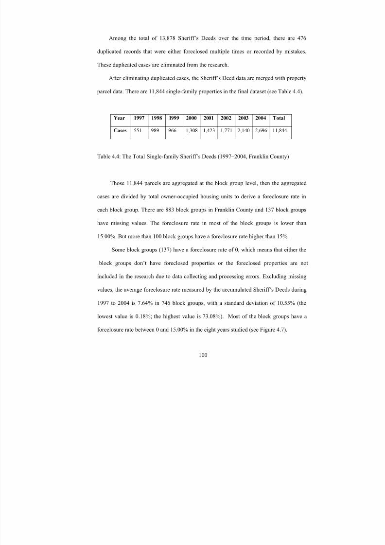
8/6/2019 Spatial Lag Regression
http://slidepdf.com/reader/full/spatial-lag-regression 114/268
100
Among the total of 13,878 Sheriff’s Deeds over the time period, there are 476
duplicated records that were either foreclosed multiple times or recorded by mistakes.
These duplicated cases are eliminated from the research.
After eliminating duplicated cases, the Sheriff’s Deed data are merged with property
parcel data. There are 11,844 single-family properties in the final dataset (see Table 4.4).
Year 1997 1998 1999 2000 2001 2002 2003 2004 Total
Cases 551 989 966 1,308 1,423 1,771 2,140 2,696 11,844
Table 4.4: The Total Single-family Sheriff’s Deeds (1997–2004, Franklin County)
Those 11,844 parcels are aggregated at the block group level, then the aggregated
cases are divided by total owner-occupied housing units to derive a foreclosure rate in
each block group. There are 883 block groups in Franklin County and 137 block groups
have missing values. The foreclosure rate in most of the block groups is lower than
15.00%. But more than 100 block groups have a foreclosure rate higher than 15%.
Some block groups (137) have a foreclosure rate of 0, which means that either the
block groups don’t have foreclosed properties or the foreclosed properties are not
included in the research due to data collecting and processing errors. Excluding missing
values, the average foreclosure rate measured by the accumulated Sheriff’s Deeds during
1997 to 2004 is 7.64% in 746 block groups, with a standard deviation of 10.55% (the
lowest value is 0.18%; the highest value is 73.08%). Most of the block groups have a
foreclosure rate between 0 and 15.00% in the eight years studied (see Figure 4.7).
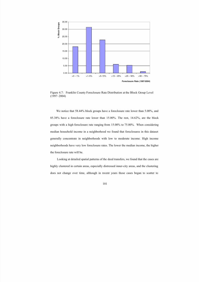
8/6/2019 Spatial Lag Regression
http://slidepdf.com/reader/full/spatial-lag-regression 115/268
101
0.00
5.00
10.00
15.00
20.00
25.00
30.00
35.00
>0 – 1% >1–5% >5–15% >15 – 25% >25 – 50% >50 – 75%
Foreclosure Rate (1997-2004)
% B
l o c k G r o u p s
Figure 4.7: Franklin County Foreclosure Rate Distribution at the Block Group Level(1997–2004)
We notice that 58.44% block groups have a foreclosure rate lower than 5.00%, and
85.38% have a foreclosure rate lower than 15.00%. The rest, 14.62%, are the block
groups with a high foreclosure rate ranging from 15.00% to 75.00%. When considering
median household income in a neighborhood we found that foreclosures in this dataset
generally concentrate in neighborhoods with low to moderate income. High income
neighborhoods have very low foreclosure rates. The lower the median income, the higher
the foreclosure rate will be.
Looking at detailed spatial patterns of the deed transfers, we found that the cases are
highly clustered in certain areas, especially distressed inner-city areas, and the clustering
does not change over time, although in recent years those cases began to scatter to

8/6/2019 Spatial Lag Regression
http://slidepdf.com/reader/full/spatial-lag-regression 116/268
102
wealthier suburbs (see Figure 4.8). This pattern is not surprising since households in
these distressed inner-city areas suffer more during economic downturns. On the other
hand, those houses might be less attractive to pre-foreclosure investors and, therefore,
many of them have to go to the Sheriff’s sales auction. So the dataset may over represent
them.
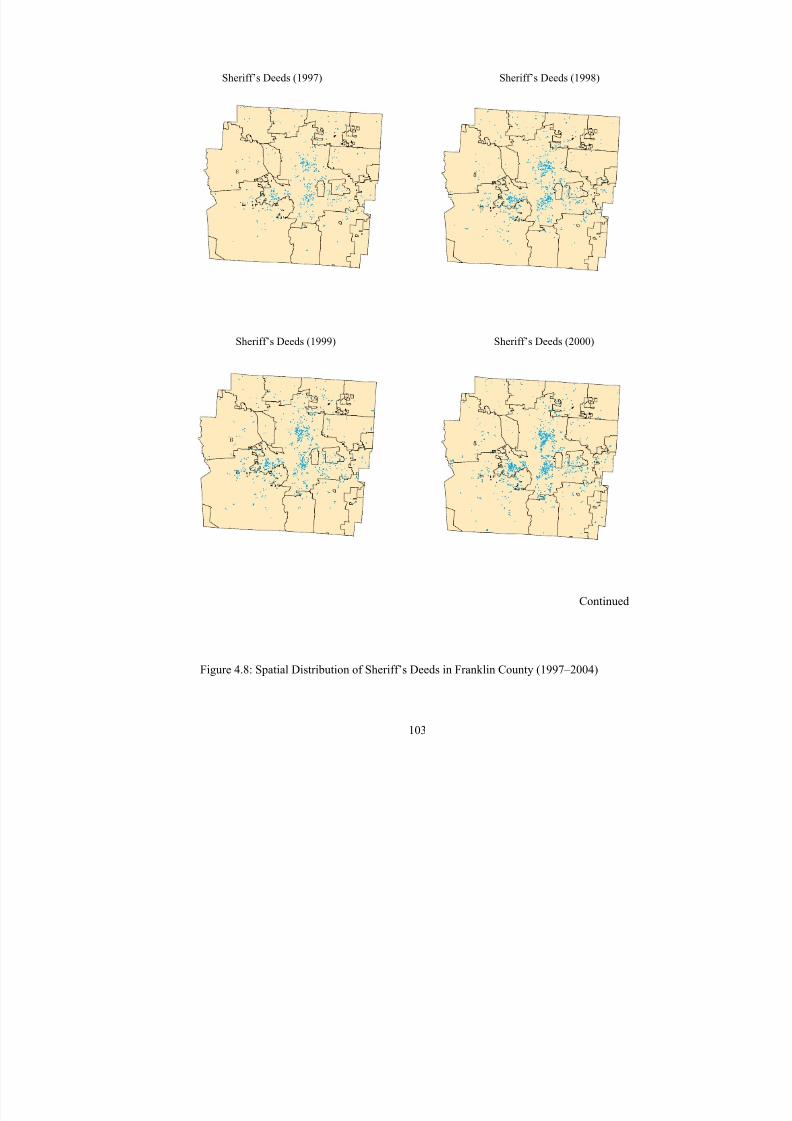
8/6/2019 Spatial Lag Regression
http://slidepdf.com/reader/full/spatial-lag-regression 117/268
103
Sheriff’s Deeds (1997) Sheriff’s Deeds (1998)
Sheriff’s Deeds (1999) Sheriff’s Deeds (2000)
Continued
Figure 4.8: Spatial Distribution of Sheriff’s Deeds in Franklin County (1997–2004)
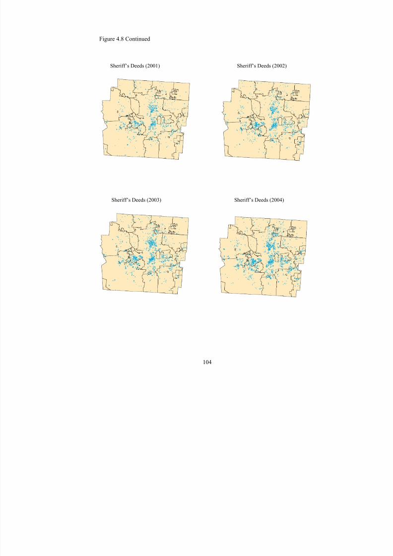
8/6/2019 Spatial Lag Regression
http://slidepdf.com/reader/full/spatial-lag-regression 118/268
104
Figure 4.8 Continued
Sheriff’s Deeds (2001) Sheriff’s Deeds (2002)
Sheriff’s Deeds (2003) Sheriff’s Deeds (2004)
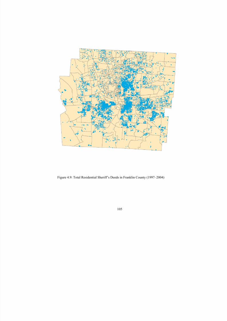
8/6/2019 Spatial Lag Regression
http://slidepdf.com/reader/full/spatial-lag-regression 119/268
105
Figure 4.9: Total Residential Sheriff’s Deeds in Franklin County (1997–2004)
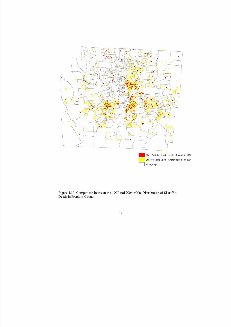
8/6/2019 Spatial Lag Regression
http://slidepdf.com/reader/full/spatial-lag-regression 120/268
106
Sheriff's Sales Deed Transfer Records in 1997
Sheriff's Sales Deed Transfer Records in 2004
blockgroup
Figure 4.10: Comparison between the 1997 and 2004 of the Distribution of Sheriff’sDeeds in Franklin County
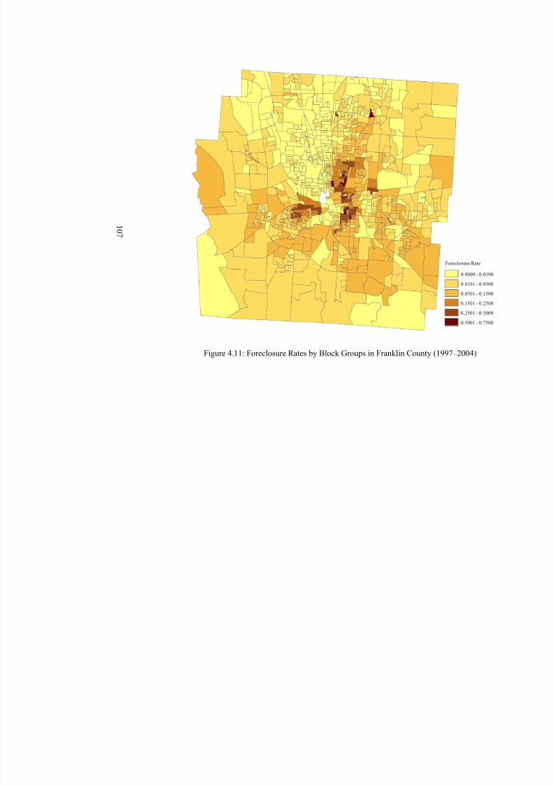
8/6/2019 Spatial Lag Regression
http://slidepdf.com/reader/full/spatial-lag-regression 121/268
1 0 7
Foreclos
0
0
0
0
0
0
Figure 4.11: Foreclosure Rates by Block Groups in Franklin County (1997–20
8/6/2019 Spatial Lag Regression
http://slidepdf.com/reader/full/spatial-lag-regression 122/268
108
Spatial Autocorrelation Analysis
Univariate and multivariate spatial autocorrelation are the two most common
analysis methods in spatial autocorrelation analysis. Univariate spatial autocorrelation
explores whether a variable is spatially autocorrelated with the same variable in adjacent
neighborhoods. Multivariate analysis explores the autocorrelation between two or more
different variables in adjacent neighborhoods. In this analysis, several sets of variables
are considered to explore whether spatial autocorrelation exists. The first set is the
univariate autocorrelation of foreclosure rates; the other sets are the bivariate
autocorrelation between foreclosure rate and median housing value of owner-occupied
housing units, percentage minority population, housing vacancy rate, and homeownership
rate. Among those bivariate autocorrelation analyses, the mutual relationship between
foreclosure rate and the selected neighborhood indicators are explored. For example, the
autocorrelation test starts with the effect of the median housing value in 2000 on
foreclosure rate between 2001 and 2004, and then the effect of foreclosure rate between
1997 and 2000 on median housing value in 2000. All the variables in this section are
standardized. All the univariate and bivariate autocorrelation tests are based on global
and local autocorrelation analyses. The significance of using local autocorrelation
analysis is to determine the relationship at the individual block group level; thus, local
autocorrelation analysis maps can be generated to illustrate those relationships.
Connectivity of Block Groups in Franklin County
Connectivity of different block groups is the basis of calculating weighting matrixes.
The connectivity of block groups is illustrated in Figure 4.12. From left to right, the
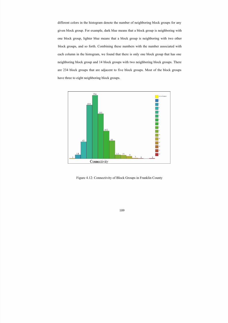
8/6/2019 Spatial Lag Regression
http://slidepdf.com/reader/full/spatial-lag-regression 123/268
109
different colors in the histogram denote the number of neighboring block groups for any
given block group. For example, dark blue means that a block group is neighboring with
one block group, lighter blue means that a block group is neighboring with two other
block groups, and so forth. Combining these numbers with the number associated with
each column in the histogram, we found that there is only one block group that has one
neighboring block group and 14 block groups with two neighboring block groups. There
are 234 block groups that are adjacent to five block groups. Most of the block groups
have three to eight neighboring block groups.
Figure 4.12: Connectivity of Block Groups in Franklin County
8/6/2019 Spatial Lag Regression
http://slidepdf.com/reader/full/spatial-lag-regression 124/268
8/6/2019 Spatial Lag Regression
http://slidepdf.com/reader/full/spatial-lag-regression 125/268
111
Foreclosure Rate and Percentage Minority Households
Contrary to the relatioonship between foreclosure and median housing value, the
relationship between foreclosure rate and racial composition of neighboring block groups
are positive, both for the correlation between racial composition and foreclosure rate
(2001– 2004) (Moran’s I = 0.4603) and the correlation between foreclosure rate (1997–
2000) on racial composition (Moran’s I = 0.4440). This means that racial composition in
2000 does are auto correlated with foreclosure rate between 2001 and 2004 in
neighboring block groups, and foreclosure rate between 1997 and 2000 is autocorrelated
with racial composition in 2000 in neighboring block groups.
Foreclosure Rate and Housing Vacancy Rate
When looking at both the correlation between housing vacancy rate and foreclosure
rate between 2001 and 2004 (Moran’s I = 0.4078) and the correlation between
foreclosure (1997–2000) and housing vacancy rate (Moran’s I = 0.4103), we found that
the relationships are positive.
Foreclosure Rate and Homeownership Rate
The autocorrelation between foreclosure rate and homeownership rate is not very
significant because Moran’s I is only slightly close to -0.15, for both the correlation
between homeownership rate in 2000 and foreclosure rate (2001–2004) and the
correlation between foreclosure rate (1997–2000) and homeownership rate in 2000.
8/6/2019 Spatial Lag Regression
http://slidepdf.com/reader/full/spatial-lag-regression 126/268
112
Local Spatial Autocorrelation
Local spatial autocorrelation explores the relationship between block groups in
terms of a certain variable (univariate), such as foreclosure rate, or the relations between
two variables (bivariate).
The analysis of local spatial autocorrelation of foreclosure rate in Franklin County
shows that a high-high spatial autocorrelation exists in the inner-city neighborhoods with
low income and a large percentage of minority population, for example, Franklinton,
Olde Town East, and Weinland Park. Those neighborhoods have high foreclosure rates
and are surrounded by ones with a high foreclosure rate. Some higher-end neighborhoods
that are adjacent to the low income ones, such as Victorian Village, Italian Village, and
German Village, present a low-high autocorrelation. Most of the northern part of the
county has a low-low autocorrelation. The autocorrelation is not significant in southern
areas. The only high-low autocorrelation in the northern suburbs of metropolitan
Columbus appears in two block groups in Dublin and Worthington. Therefore, the
neighborhoods with a significant local Moran’s I are either located in inner-city low
income neighborhoods (high-high autocorrelation), inner-city median to high income
neighborhoods (low-high autocorrelation), or suburban median to high income
neighborhoods (low-low autocorrelation). The southern part of the County has mixed-
income neighborhoods and the local Moran’s I is not significant.
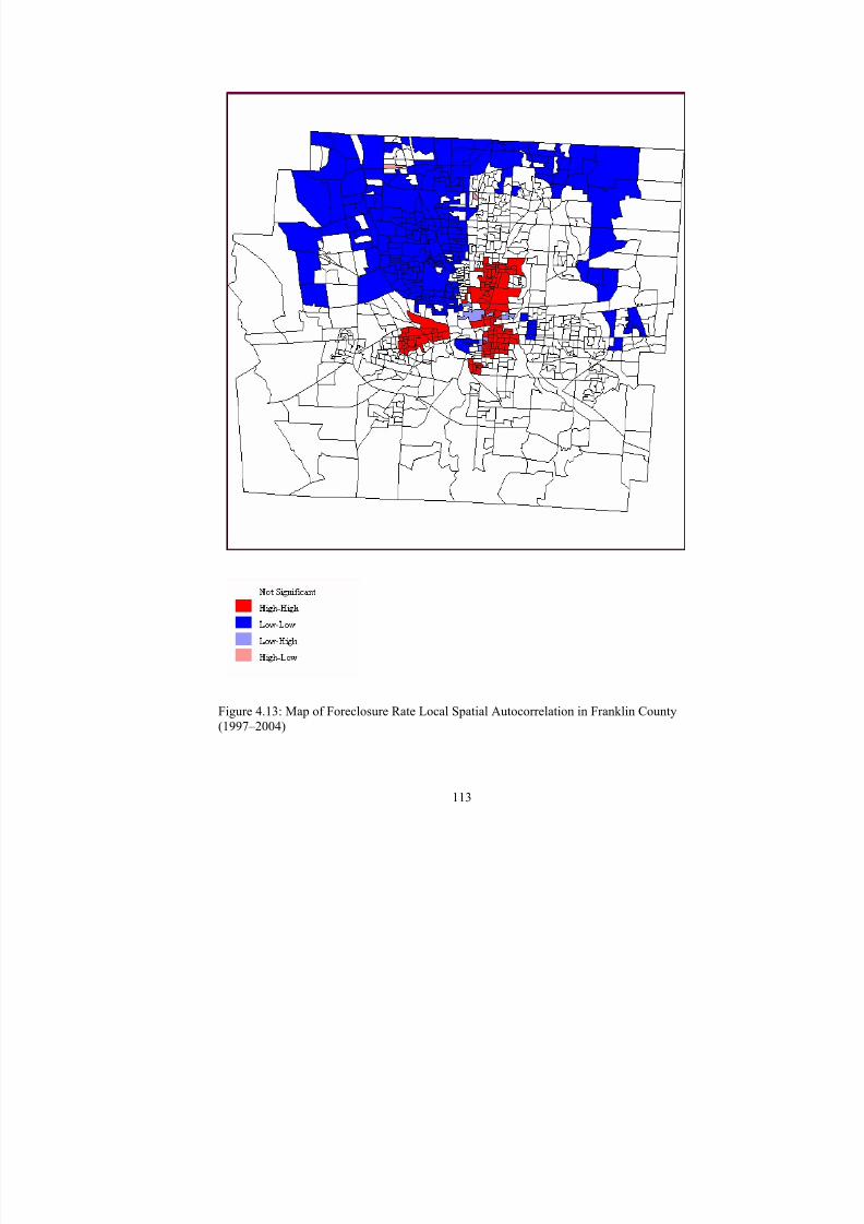
8/6/2019 Spatial Lag Regression
http://slidepdf.com/reader/full/spatial-lag-regression 127/268
113
Figure 4.13: Map of Foreclosure Rate Local Spatial Autocorrelation in Franklin County(1997–2004)
8/6/2019 Spatial Lag Regression
http://slidepdf.com/reader/full/spatial-lag-regression 128/268
114
Temporal Change in Selected Neighborhood Variables
From 1990 to 2000, Franklin County experienced rapid changes in some
neighborhood characteristics. Generally speaking, the most significant changes were an
increased percentage of minority population and thus a decreased percentage of white
population, increased housing cost burden, and increased total housing units. The
countywide change and the change by different levels of foreclosure rate are summarized
in the following sections.
Demographic Characteristics
For the entire county, the black population increased by 3.92% points and the
minority population in general increased by 8.03% points. Thus, the white population
decreased by 8.00% points. The county is more diverse than ever, and the outflow of the
white population continues to be a significant phenomenon. However, the most
significant increase of minority population and decrease of white population is
concentrated in the neighborhoods with a foreclosure rate of 5–15% (see Table 4.5).
Economic Characteristics
It is interesting to note that from 1990 to 2000 the unemployment rate decreased by
0.90% points, and for those block groups with observations the decrease is even bigger
(1.30% points). The population employed in management occupations increased
dramatically by 20.22% points, and the biggest increase is in those neighborhoods with
the lowest foreclosure rate. The population employed in service occupations increased by
2.55% points, but there is no obvious patterns observed at different levels of foreclosure
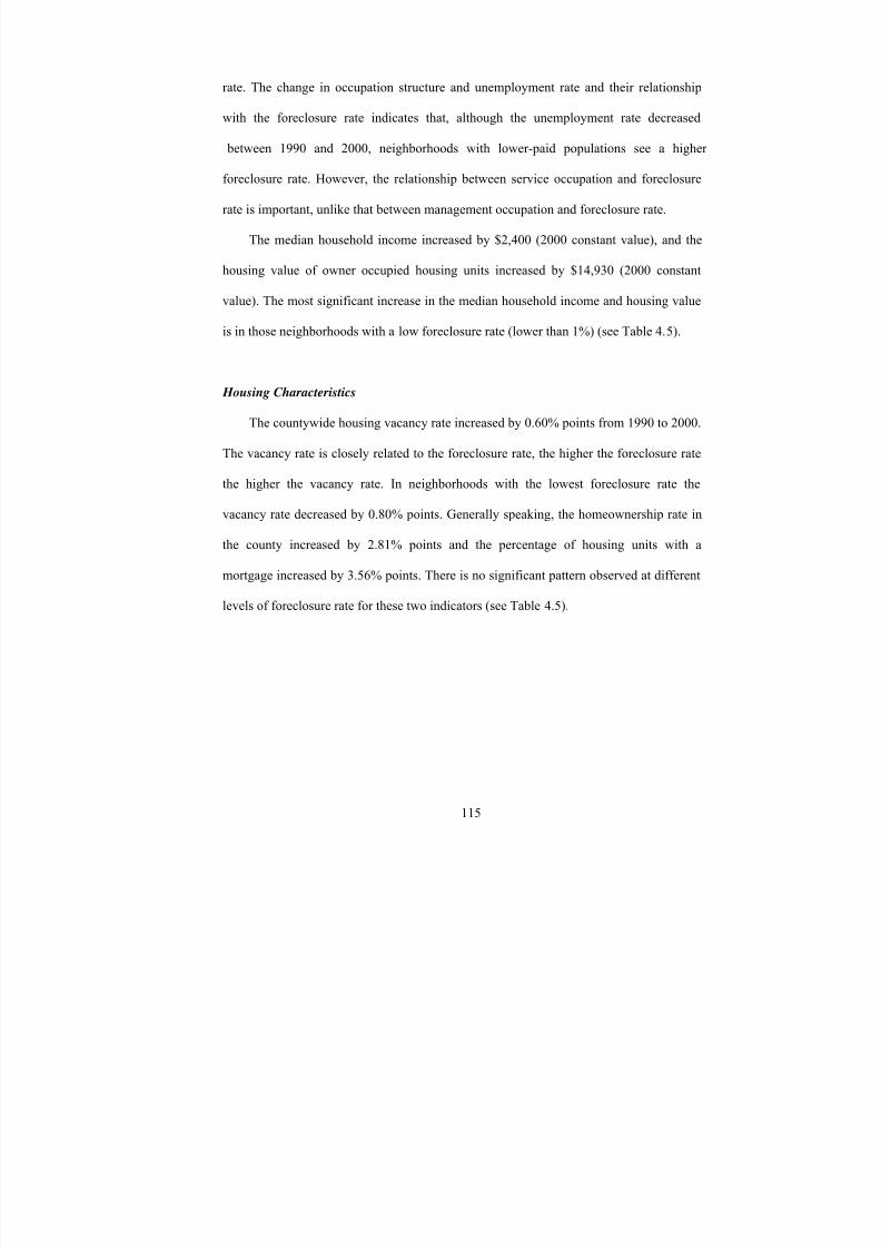
8/6/2019 Spatial Lag Regression
http://slidepdf.com/reader/full/spatial-lag-regression 129/268
115
rate. The change in occupation structure and unemployment rate and their relationship
with the foreclosure rate indicates that, although the unemployment rate decreased
between 1990 and 2000, neighborhoods with lower-paid populations see a higher
foreclosure rate. However, the relationship between service occupation and foreclosure
rate is important, unlike that between management occupation and foreclosure rate.
The median household income increased by $2,400 (2000 constant value), and the
housing value of owner occupied housing units increased by $14,930 (2000 constant
value). The most significant increase in the median household income and housing value
is in those neighborhoods with a low foreclosure rate (lower than 1%) (see Table 4.5).
Housing Characteristics
The countywide housing vacancy rate increased by 0.60% points from 1990 to 2000.
The vacancy rate is closely related to the foreclosure rate, the higher the foreclosure rate
the higher the vacancy rate. In neighborhoods with the lowest foreclosure rate the
vacancy rate decreased by 0.80% points. Generally speaking, the homeownership rate in
the county increased by 2.81% points and the percentage of housing units with a
mortgage increased by 3.56% points. There is no significant pattern observed at different
levels of foreclosure rate for these two indicators (see Table 4.5).
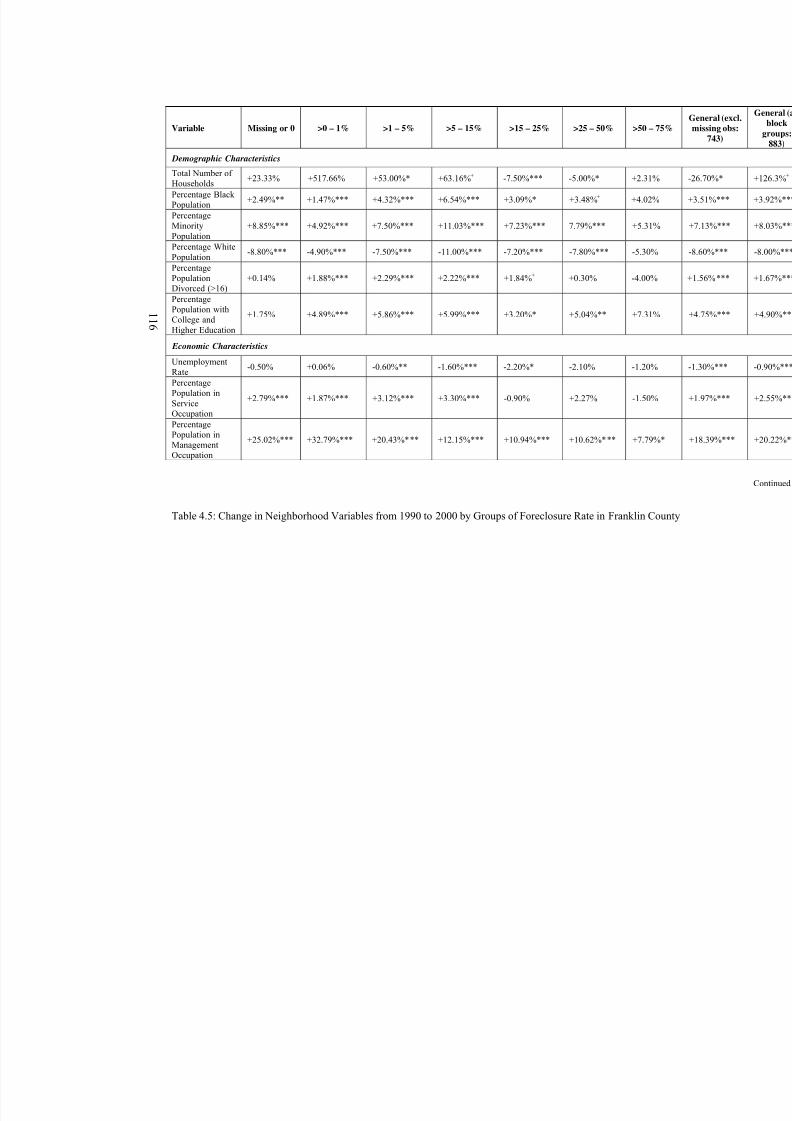
8/6/2019 Spatial Lag Regression
http://slidepdf.com/reader/full/spatial-lag-regression 130/268
1 1 6
Variable Missing or 0 >0 – 1% >1 – 5% >5 – 15% >15 – 25% >25 – 50% >50 – 7
Demographic Characteristics
Total Number of Households
+23.33% +517.66% +53.00%* +63.16%+ -7.50%*** -5.00%* +2.31%
Percentage Black Population
+2.49%** +1.47%*** +4.32%*** +6.54%*** +3.09%* +3.48%+ +4.02%
PercentageMinorityPopulation
+8.85%*** +4.92%*** +7.50%*** +11.03%*** +7.23%*** 7.79%*** +5.31%
Percentage WhitePopulation
-8.80%*** -4.90%*** -7.50%*** -11.00%*** -7.20%*** -7.80%*** -5.30%
PercentagePopulationDivorced (>16)
+0.14% +1.88%*** +2.29%*** +2.22%*** +1.84%+ +0.30% -4.00%
PercentagePopulation withCollege andHigher Education
+1.75% +4.89%*** +5.86%*** +5.99%*** +3.20%* +5.04%** +7.31%
Economic Characteristics
UnemploymentRate
-0.50% +0.06% -0.60%** -1.60%*** -2.20%* -2.10% -1.20%
PercentagePopulation inServiceOccupation
+2.79%*** +1.87%*** +3.12%*** +3.30%*** -0.90% +2.27% -1.50%
PercentagePopulation inManagement
Occupation
+25.02%*** +32.79%*** +20.43%*** +12.15%*** +10.94%*** +10.62%*** +7.79%*
Table 4.5: Change in Neighborhood Variables from 1990 to 2000 by Groups of Foreclosure Rate in Franklin Co
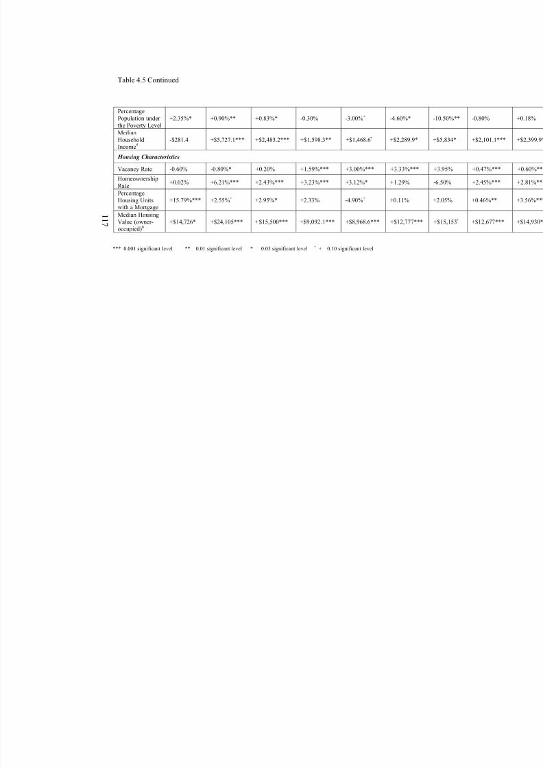
8/6/2019 Spatial Lag Regression
http://slidepdf.com/reader/full/spatial-lag-regression 131/268
1 1 7
Table 4.5 Continued
PercentagePopulation under the Poverty Level
+2.35%* +0.90%** +0.83%* -0.30% -3.00%+ -4.60%* -10.50%
MedianHouseholdIncome5
-$281.4 +$5,727.1*** +$2,483.2*** +$1,598.3** +$1,468.6+ +$2,289.9* +$5,834
Housing Characteristics
Vacancy Rate -0.60% -0.80%* +0.20% +1.59%*** +3.00%*** +3.33%*** +3.95%
HomeownershipRate
+0.02% +6.21%*** +2.43%*** +3.23%*** +3.12%* +1.29% -6.50%
PercentageHousing Units
with a Mortgage
+15.79%*** +2.55%+ +2.95%* +2.33% -4.90%+ +0.11% +2.05%
Median HousingValue (owner-occupied)6
+$14,726* +$24,105*** +$15,500*** +$9,092.1*** +$8,968.6*** +$12,777*** +$15,153
*** 0.001 significant level ** 0.01 significant level * 0.05 significant level + + 0.10 significant level
8/6/2019 Spatial Lag Regression
http://slidepdf.com/reader/full/spatial-lag-regression 132/268
118
Cuyahoga County, Ohio
General Description
In terms of Sheriff’s Deeds, the Cuyahoga County Recorder’s Office provides the
most complete records of Sheriff’s sales data among those counties I examined. There are
more than 30 years of historical data on Sheriff’s Deeds. Since 1983 parcel IDs have been
incorporated into the index file, which can be used as a 21-year time series record of
Sheriff’s sales data.
Sheriff's Deeds
0
500
1000
1500
2000
2500
3000
1 9 6 5
1 9 6 7
1 9 6 9
1 9 7 1
1 9 7 3
1 9 7 5
1 9 7 7
1 9 7 9
1 9 8 1
1 9 8 3
1 9 8 5
1 9 8 7
1 9 8 9
1 9 9 1
1 9 9 3
1 9 9 5
1 9 9 7
1 9 9 9
2 0 0 1
2 0 0 3
Year
Figure 4.14: Total Sheriff’s Deeds in Cuyahoga County (1965–2004)
The 21-year span is shown in Figure 4.14 for reference. However, to compare the
two counties this research uses those sales between 1997 and 2004. Over those eight
years, there were 54,584 total new foreclosure filings and 16,705 recorded Sheriff’s
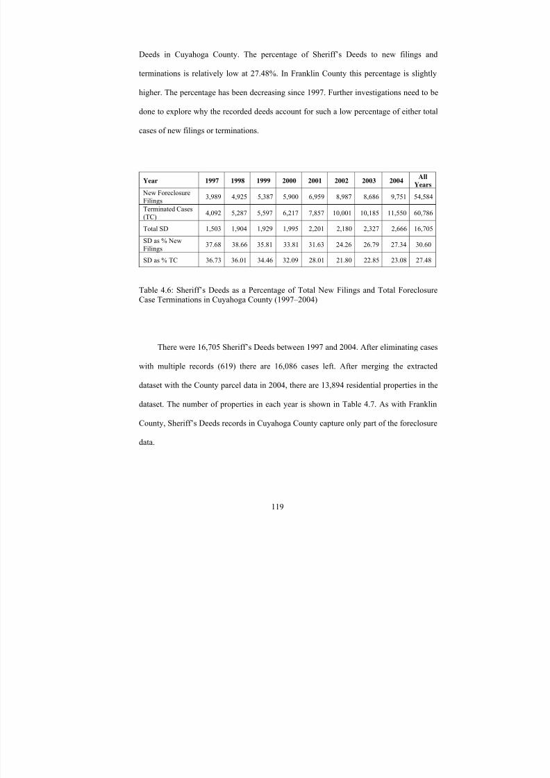
8/6/2019 Spatial Lag Regression
http://slidepdf.com/reader/full/spatial-lag-regression 133/268
119
Deeds in Cuyahoga County. The percentage of Sheriff’s Deeds to new filings and
terminations is relatively low at 27.48%. In Franklin County this percentage is slightly
higher. The percentage has been decreasing since 1997. Further investigations need to be
done to explore why the recorded deeds account for such a low percentage of either total
cases of new filings or terminations.
Year 1997 1998 1999 2000 2001 2002 2003 2004All
Years
New ForeclosureFilings
3,989 4,925 5,387 5,900 6,959 8,987 8,686 9,751 54,584
Terminated Cases(TC)
4,092 5,287 5,597 6,217 7,857 10,001 10,185 11,550 60,786
Total SD 1,503 1,904 1,929 1,995 2,201 2,180 2,327 2,666 16,705
SD as % NewFilings
37.68 38.66 35.81 33.81 31.63 24.26 26.79 27.34 30.60
SD as % TC 36.73 36.01 34.46 32.09 28.01 21.80 22.85 23.08 27.48
Table 4.6: Sheriff’s Deeds as a Percentage of Total New Filings and Total ForeclosureCase Terminations in Cuyahoga County (1997–2004)
There were 16,705 Sheriff’s Deeds between 1997 and 2004. After eliminating cases
with multiple records (619) there are 16,086 cases left. After merging the extracted
dataset with the County parcel data in 2004, there are 13,894 residential properties in the
dataset. The number of properties in each year is shown in Table 4.7. As with Franklin
County, Sheriff’s Deeds records in Cuyahoga County capture only part of the foreclosure
data.
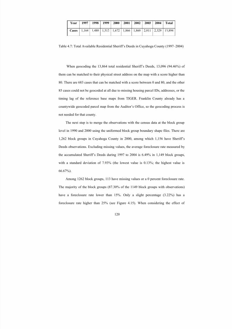
8/6/2019 Spatial Lag Regression
http://slidepdf.com/reader/full/spatial-lag-regression 134/268
120
Year 1997 1998 1999 2000 2001 2002 2003 2004 Total
Cases 1,164 1,480 1,512 1,672 1,866 1,860 2,011 2,329 13,894
Table 4.7: Total Available Residential Sheriff’s Deeds in Cuyahoga County (1997–2004)
When geocoding the 13,864 total residential Sheriff’s Deeds, 13,096 (94.46%) of
them can be matched to their physical street address on the map with a score higher than
80. There are 683 cases that can be matched with a score between 0 and 80, and the other
85 cases could not be geocoded at all due to missing housing parcel IDs, addresses, or the
timing lag of the reference base maps from TIGER. Franklin County already has a
countywide geocoded parcel map from the Auditor’s Office, so the geocoding process is
not needed for that county.
The next step is to merge the observations with the census data at the block group
level in 1990 and 2000 using the uniformed block group boundary shape files. There are
1,262 block groups in Cuyahoga County in 2000, among which 1,156 have Sheriff’s
Deeds observations. Excluding missing values, the average foreclosure rate measured by
the accumulated Sheriff’s Deeds during 1997 to 2004 is 6.49% in 1,149 block groups,
with a standard deviation of 7.93% (the lowest value is 0.13%; the highest value is
66.67%).
Among 1262 block groups, 113 have missing values or a 0 percent foreclosure rate.
The majority of the block groups (87.30% of the 1149 block groups with observations)
have a foreclosure rate lower than 15%. Only a slight percentage (3.22%) has a
foreclosure rate higher than 25% (see Figure 4.15). When considering the effect of
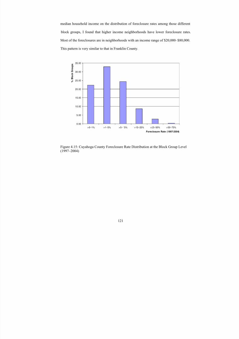
8/6/2019 Spatial Lag Regression
http://slidepdf.com/reader/full/spatial-lag-regression 135/268
121
median household income on the distribution of foreclosure rates among those different
block groups, I found that higher income neighborhoods have lower foreclosure rates.
Most of the foreclosures are in neighborhoods with an income range of $20,000–$80,000.
This pattern is very similar to that in Franklin County.
0.00
5.00
10.00
15.00
20.00
25.00
30.00
35.00
>0–1% >1–5% >5–15% >15–25% >25–50% >50–75%
Foreclosure Rate (1997-2004)
% B
l o c k G r o u p s
Figure 4.15: Cuyahoga County Foreclosure Rate Distribution at the Block Group Level(1997–2004)

8/6/2019 Spatial Lag Regression
http://slidepdf.com/reader/full/spatial-lag-regression 136/268
1 2 2
Sheriff’s Deeds (1997) Sheriff’s Deeds (1998)
Sheriff’s Deeds (1999) Sheriff’s Deeds (2000)
Figure 4.16: Spatial Distribution of Sheriff’s Deeds in Cuyahoga County (1997–2004)

8/6/2019 Spatial Lag Regression
http://slidepdf.com/reader/full/spatial-lag-regression 137/268
1 2 3
Figure 4.16 Continued
Sheriff’s Deeds (2001) Sheriff’s Deeds (2002)
Sheriff’s Deeds (2003) Sheriff’s Deeds (2004)
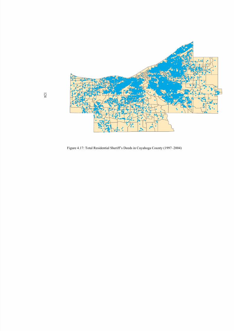
8/6/2019 Spatial Lag Regression
http://slidepdf.com/reader/full/spatial-lag-regression 138/268
1 2 4
Figure 4.17: Total Residential Sheriff’s Deeds in Cuyahoga County (1997–2004)
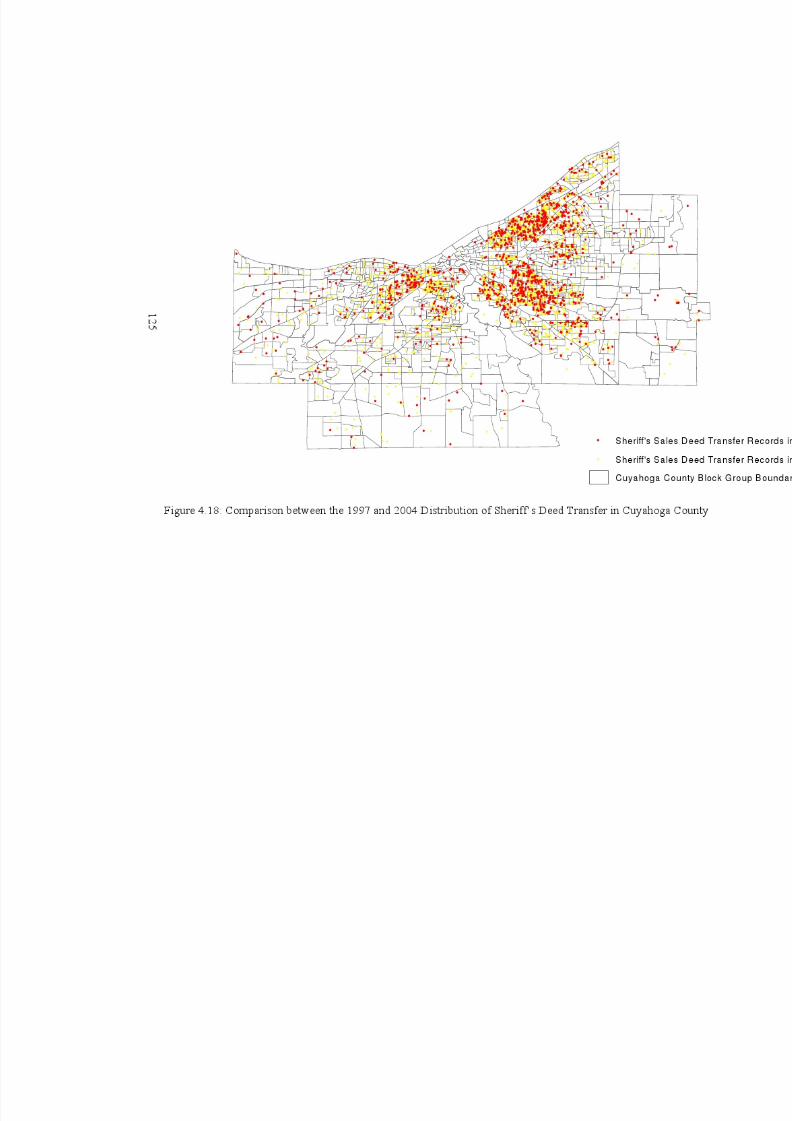
8/6/2019 Spatial Lag Regression
http://slidepdf.com/reader/full/spatial-lag-regression 139/268
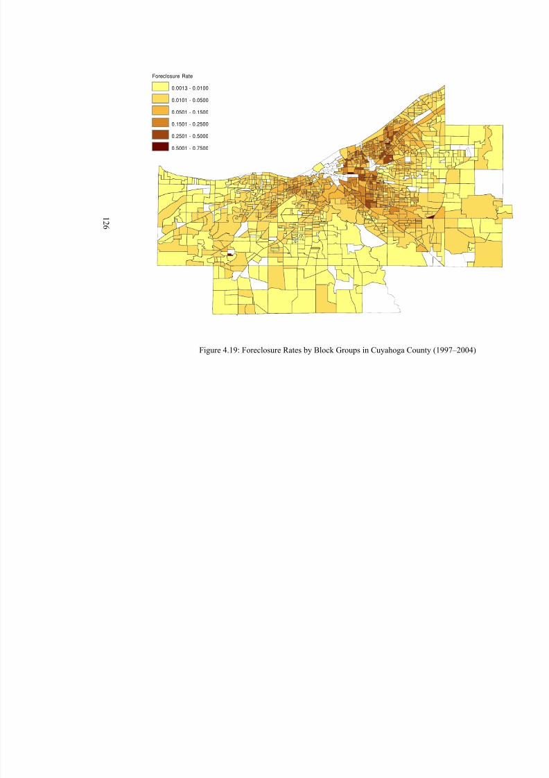
8/6/2019 Spatial Lag Regression
http://slidepdf.com/reader/full/spatial-lag-regression 140/268
1 2 6
Foreclosure Rate
0.0013 - 0.0100
0.0101 - 0.0500
0.0501 - 0.1500
0.1501 - 0.2500
0.2501 - 0.5000
0.5001 - 0.7500
Figure 4.19: Foreclosure Rates by Block Groups in Cuyahoga County (1997–2
8/6/2019 Spatial Lag Regression
http://slidepdf.com/reader/full/spatial-lag-regression 141/268
127
Foreclosures in 1983–1989
In order to create necessary time lags when exploring how foreclosures are related
to neighborhood change, Sheriff’s Deeds in 1983–1989 in Cuyahoga County are used.
There were 9,185 Sheriff’s Deeds during this time period. After getting rid of the
duplicated cases there are 8,900 deeds left. Those properties were then merged with 1988
Cuyahoga County parcel data7. There are 7,872 residential properties. After geocoding
there left 7,412 valid cases (460 addresses could not be geocoded, thus could not merge
with the census data). Then those cases are aggregated at block group level, merged with
the census block and place data, and divided by 1990 owner-occupied housing units in a
block group to derive foreclosure rates. The aggregated foreclosure rate in 1983–1989 in
Cuyahoga County is 3.67% (including those block groups with 0 foreclosures) based on
1221 block groups. Forty-one block groups have missing values. The highest foreclosure
rate is 59.02%. The standard deviation of foreclosure rates is 5.50%. Figure 4.20 is the
detailed map of the distribution of foreclosure rates at the block group level in Cuyahoga
County in the time period.

8/6/2019 Spatial Lag Regression
http://slidepdf.com/reader/full/spatial-lag-regression 142/268
1 2 8
Foreclosure Rate
0.0000 - 0.0100
0.0101 - 0.0500
0.0501 - 0.1500
0.1501 - 0.2500
0.2501 - 0.5000
0.5001 - 0.7500
Figure 4.20: Foreclosure Rates by Block Groups in Cuyahoga County (1983-1

8/6/2019 Spatial Lag Regression
http://slidepdf.com/reader/full/spatial-lag-regression 143/268
129
Spatial Autocorrelation Analysis
As with Franklin County, both global and local spatial autocorrelation are analyzed
for Cuyahoga County. Univariate and multivariate autocorrelation are analyzed to
explore whether the foreclosure rate in one neighborhood is autocorrelated with the
foreclosure rate in adjacent neighborhoods, and whether the foreclosure rate in one
neighborhood is autocorrelated with other neighborhood indicators in adjacent
neighborhoods.
Connectivity of Block Groups in Cuyahoga County
In Cuyahoga County, most of the block groups are neighboring three to eight other
block groups. There are 350 block groups that have five neighboring block groups. Only
a few block groups have only one and two adjacent block groups; and only a few have
more than 10 adjacent block groups. The weighting matrix is derived based on the
connectivity of block groups and thus is used as the basis for further spatial regression
analysis.

8/6/2019 Spatial Lag Regression
http://slidepdf.com/reader/full/spatial-lag-regression 144/268
130
Figure 4.21: Connectivity of Block Groups in Cuyahoga County
Global Spatial Autocorrelation
Foreclosure Rate
The spatial autocorrelation of foreclosure rates in different neighborhoods is
significant with a Moran’s I of 0.5588. This means that foreclosure rate is autocorrelated
with the foreclosure rate in neighboring block groups. Therefore, the spatial distribution
of foreclosure rates is not random but is highly clustered. Similar patterns show in the
foreclosure rates between 1997 and 2000 (Moran’s I = 0.4339), and between 2001 and
2004 (Moran’s I = 0.5647). This means that foreclosures become more clustered after
2000.
Foreclosure Rate and Median Housing Value
Looking at the relationship between median housing value in 1990 and foreclosure
rate between 1997 and 2004, we found that these variables are negatively autocorrelated
8/6/2019 Spatial Lag Regression
http://slidepdf.com/reader/full/spatial-lag-regression 145/268
131
(Moran’s I = -0.3714). This means that median housing value in one neighborhood is
negatively autocorrelated with foreclosure rate in neighboring block groups. Similar
patterns exist when investigating how foreclosure rate between 1997 and 2004 is
autocorrelated with median housing value in 2000 (Moran’s I = -0.3068). These simple
relationships between foreclosure rate and median housing value indicate that those two
variables are not only closely related to each other but also have a spatial relationship.
Median housing value is autocorrelated with foreclosure rate and vise versa; foreclosure
rate is autocorrelated with median housing value in adjacent neighborhoods.
Foreclosure Rate and Percentage Minority Population
Contrary to the relationships between foreclosure and median housing value, the
relationships between foreclosure rate and racial composition of neighboring block
groups are positive, both for the correlation between racial composition and foreclosure
rate (2001–2004) (Moran’s I = 0.5752) and the correlation between foreclosure rate
(1997–2000) and racial composition (Moran’s I = 0.5211). This means that the 1990
racial transition is autocorrelated with foreclosure rate between 1997 and 2004 in
neighboring block groups, and foreclosure rate between 1997 and 2004 is autocorrelated
with racial composition in 2000 in neighboring block groups.
Foreclosure Rate and Housing Vacancy Rate
When looking at both the correlation between housing vacancy rate and foreclosure
rate between 2001 and 2004 (Moran’s I = 0.4170) and the correlation between
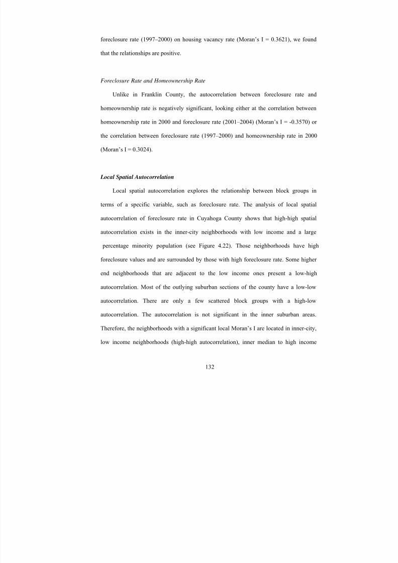
8/6/2019 Spatial Lag Regression
http://slidepdf.com/reader/full/spatial-lag-regression 146/268
132
foreclosure rate (1997–2000) on housing vacancy rate (Moran’s I = 0.3621), we found
that the relationships are positive.
Foreclosure Rate and Homeownership Rate
Unlike in Franklin County, the autocorrelation between foreclosure rate and
homeownership rate is negatively significant, looking either at the correlation between
homeownership rate in 2000 and foreclosure rate (2001–2004) (Moran’s I = -0.3570) or
the correlation between foreclosure rate (1997–2000) and homeownership rate in 2000
(Moran’s I = 0.3024).
Local Spatial Autocorrelation
Local spatial autocorrelation explores the relationship between block groups in
terms of a specific variable, such as foreclosure rate. The analysis of local spatial
autocorrelation of foreclosure rate in Cuyahoga County shows that high-high spatial
autocorrelation exists in the inner-city neighborhoods with low income and a large
percentage minority population (see Figure 4.22). Those neighborhoods have high
foreclosure values and are surrounded by those with high foreclosure rate. Some higher
end neighborhoods that are adjacent to the low income ones present a low-high
autocorrelation. Most of the outlying suburban sections of the county have a low-low
autocorrelation. There are only a few scattered block groups with a high-low
autocorrelation. The autocorrelation is not significant in the inner suburban areas.
Therefore, the neighborhoods with a significant local Moran’s I are located in inner-city,
low income neighborhoods (high-high autocorrelation), inner median to high income

8/6/2019 Spatial Lag Regression
http://slidepdf.com/reader/full/spatial-lag-regression 147/268
133
neighborhoods (low-high autocorrelation), or outlying suburban median to high income
neighborhoods (low-low autocorrelation).
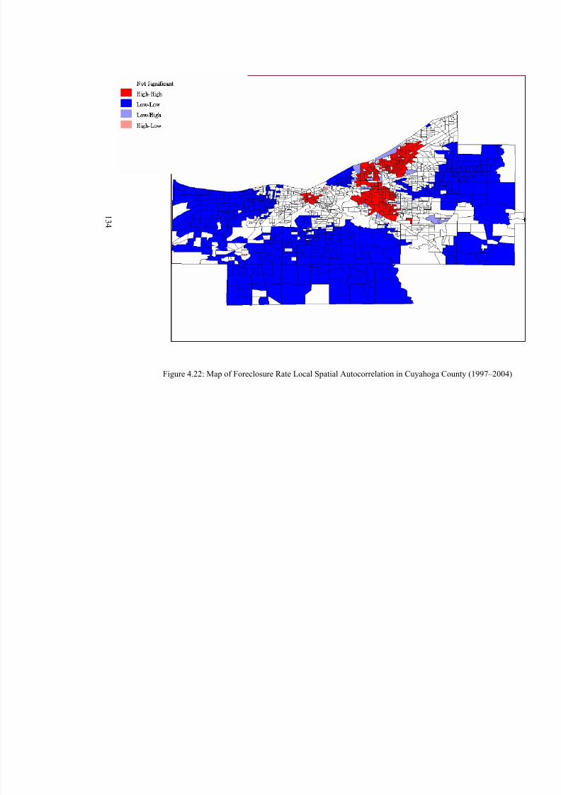
8/6/2019 Spatial Lag Regression
http://slidepdf.com/reader/full/spatial-lag-regression 148/268
1 3 4
Figure 4.22: Map of Foreclosure Rate Local Spatial Autocorrelation in Cuyahoga County (
8/6/2019 Spatial Lag Regression
http://slidepdf.com/reader/full/spatial-lag-regression 149/268
135
Temporal Change in Selected Neighborhood Variables
Generally speaking, the pattern of change in neighborhood variables in Cuyahoga
County is very similar to that in Franklin County. The percentage of black and minority
population is increasing and the percentage of white population is decreasing. The
population is more educated than in 1990. The housing vacancy rate has increased and
the housing cost burden for those with a mortgage has increased dramatically (see Table
4.8).
Demographic Characteristics
Unlike Franklin County, the total number of households decreased slightly (0.42%)
for Cuyahoga County. The higher the neighborhood foreclosure rate the higher the
decrease in household formations. Neighborhoods with increased number of total
households are those with a relatively low foreclosure rate (less than 1%). All other types
of neighborhoods experienced loss of households.
There is more increase in black population and less increase in overall percentage
minority population than in Franklin County. This might mean that the County is not as
attractive to all minorities as Franklin County, while it is more attractive to black
population. The biggest increase of black and minority populations concentrate on those
neighborhoods with a foreclosure rate of 5–15%. The percentage of white population has
decreased by 8.30% points, which is similar to the decrease in Franklin County. The
biggest decrease in white population is observed in the neighborhoods with foreclosure
rates of 5–50%.
8/6/2019 Spatial Lag Regression
http://slidepdf.com/reader/full/spatial-lag-regression 150/268
136
Compared to 1990, the divorced population increased by 1.18% points, but there is
no significant pattern observed at different levels of foreclosure rate. In most block
groups the education level of the residents has increased; for the entire county the
increase is 7.05% points for the population with college and higher education. The only
neighborhoods with a decrease in educational attainment are those several with the
highest foreclosure rate (50–75%).
Economic Characteristics
The unemployment rate in Cuyahoga County decreased by 1.90% points compared
to that in 1990. As with Franklin County, the percentage population employed in a
management occupation is highly related to foreclosure rate, where the higher the
foreclosure rate the lower the increase in percentage population in management
occupations. The percentage population employed in service occupations increased
slightly (by 1.77% points). The median household income increased $1,545.6 (2000
constant value), which is much lower than the increase in Franklin County.
Housing Characteristics
The increase in the median value of owner-occupied housing units is about $16,363.
The housing vacancy rate increased by 0.66% points, and the pattern is not significant
when considering its relationship with foreclosure rate. The homeownership rate
increased by 2.36% points. Compared to Franklin County, the percentage increase of
housing units with a mortgage is much larger at 8.36% points (It is 3.56% points for
Franklin County).
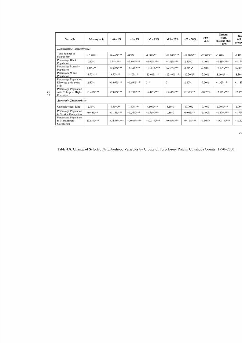
8/6/2019 Spatial Lag Regression
http://slidepdf.com/reader/full/spatial-lag-regression 151/268
1
3 7
Variable Missing or 0 >0 – 1% >1 – 5% >5 – 15% >15 – 25% >25 – 50%
Demographic Characteristics
Total number of Households
-15.40% +6.46%*** -0.9% -4.90%** -11.80%*** -17.10%** -3
Percentage Black Population
-1.60% 0.74%*** +3.89%*** +6.99%*** +4.51%*** -2.50% -4
Percentage MinorityPopulation
0.11%** +2.62%*** +6.94%*** +10.13%*** +6.56%*** -0.20%* -2
Percentage WhitePopulation
-6.70%** -3.70%*** -8.80%*** -13.60%*** -13.40%*** -10.20%* -2
Percentage PopulationDivorced (>16 yearsold)
-2.60% +1.99%*** +1.66%*** 0** 0* -2.80% -9
Percentage Population
with College or Higher Education
+3.45%*** +7.05%*** +6.99%*** +6.44%*** +5.64%*** +2.30%** -1
Economic Characteristics
Unemployment Rate -2.90% -0.80%** -1.40%*** -4.10%*** -3.10% -10.70% -7
Percentage Populationin Service Occupation
+0.45%** +1.15%*** +1.26%*** +1.71%*** -0.80% +0.03%** -3
Percentage Populationin ManagementOccupation
23.63%*** +24.68%*** +20.66%*** +12.77%*** +9.67%*** +9.11%*** -3
Table 4.8: Change of Selected Neighborhood Variables by Groups of Foreclosure Rate in Cuyahoga
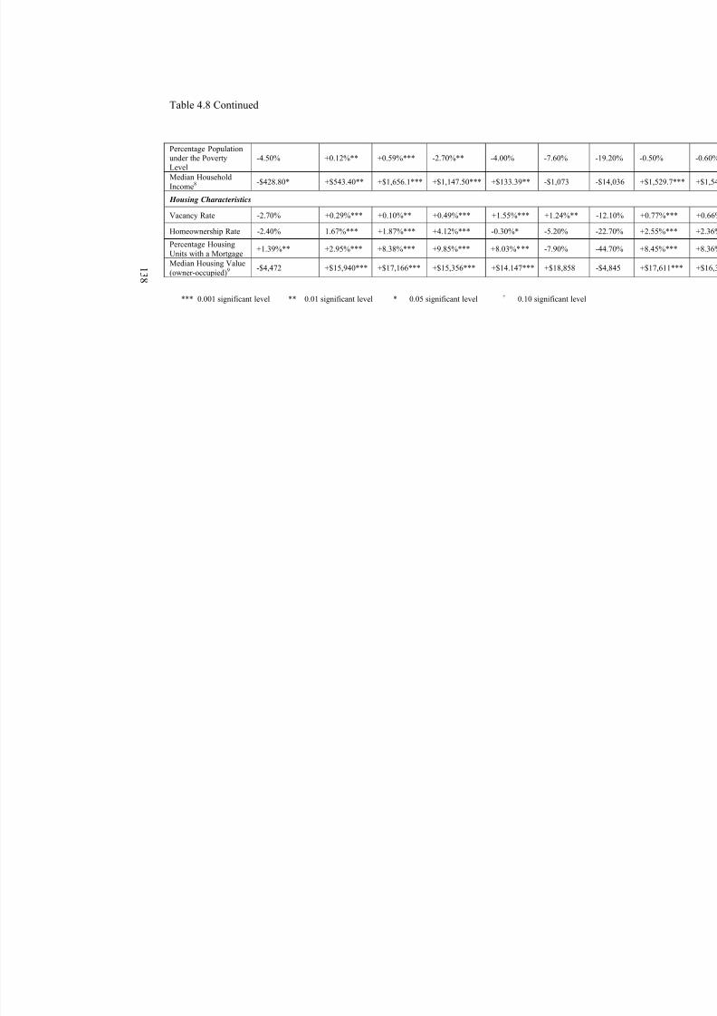
8/6/2019 Spatial Lag Regression
http://slidepdf.com/reader/full/spatial-lag-regression 152/268
1
3 8
Table 4.8 Continued
Percentage Populationunder the PovertyLevel
-4.50% +0.12%** +0.59%*** -2.70%** -4.00% -7.60% -1
Median HouseholdIncome8
-$428.80* +$543.40** +$1,656.1*** +$1,147.50*** +$133.39** -$1,073 -$
Housing Characteristics
Vacancy Rate -2.70% +0.29%*** +0.10%** +0.49%*** +1.55%*** +1.24%** -1
Homeownership Rate -2.40% 1.67%*** +1.87%*** +4.12%*** -0.30%* -5.20% -2
Percentage HousingUnits with a Mortgage
+1.39%** +2.95%*** +8.38%*** +9.85%*** +8.03%*** -7.90% -4
Median Housing Value
(owner-occupied)9
-$4,472 +$15,940*** +$17,166*** +$15,356*** +$14.147*** +$18,858 -$
*** 0.001 significant level ** 0.01 significant level * 0.05 significant level + 0.10 significant level
8/6/2019 Spatial Lag Regression
http://slidepdf.com/reader/full/spatial-lag-regression 153/268
139
Conclusions
Simple statistical and spatial analysis shows that in both counties new foreclosure
filings and the foreclosure rate measured in this study have increased dramatically since
the mid 1990s. Foreclosures have concentrated in low to moderate income and inner-city
neighborhoods, although suburban areas have seen some increases in recent years. In
both counties foreclosures become a broader county-wide issue over time. Among the
new foreclosure filings there are only about a quarter to a third that finished the
foreclosure process. The reason why many of those new filings did not terminate as
foreclosed properties remains unknown.
The economic situation of the two counties is different with Franklin County having
a stronger economy and a younger and better educated population. Cuyahoga County has
a higher homeownership rate than in Franklin County. When aggregating data and
considering all block groups, the residential foreclosure rate from 1997 to 2004 in
Franklin County is 6.47% and in Cuyahoga County is 6.49%. Block groups with
foreclosures are usually those with a median income between $20,000 and $80,000. The
study found that the educational levels of the population in both counties have increased
greatly, but those neighborhoods with the highest foreclosure rate (50–75%) show
decreases in educational attainment.
One of the significant findings is that in both counties the percentage of the white
population decreased by about 8% between 1990 and 2000. The biggest increase of
minority population occured in those neighborhoods with foreclosure rates in the range of
5–15%. When considering the effect of occupation on foreclosures, the research found
that the percentage population in management and executive jobs negatively relates to the

8/6/2019 Spatial Lag Regression
http://slidepdf.com/reader/full/spatial-lag-regression 154/268
140
foreclosure rate. The neighborhood unemployment rate is not significantly related to
foreclosures in either county.
The housing vacancy rate has been found to be positively related to the foreclosure
rate. The pace of real income increase does not match the increase in housing value,
leaving more people vulnerable to foreclosures.
Spatial autocorrelation shows that foreclosures clustered in both counties.
Foreclosures in one block group are autocorrelated with foreclosures in neighboring
block groups. Foreclosures are positively autocorrelated with percentage minority
population and housing vacancy rate in neighboring block groups. Foreclosures are
negatively autocorrelated with median housing value of owner-occupied housing units in
neighboring block groups. In Franklin County foreclosures and homeownership rate is
not autocorrelated, but in Cuyahoga County the two are significantly autocorrelated. All
those findings indicate that foreclosures and some neighborhood characteristics are
autocorrelated with each other in neighboring block groups.
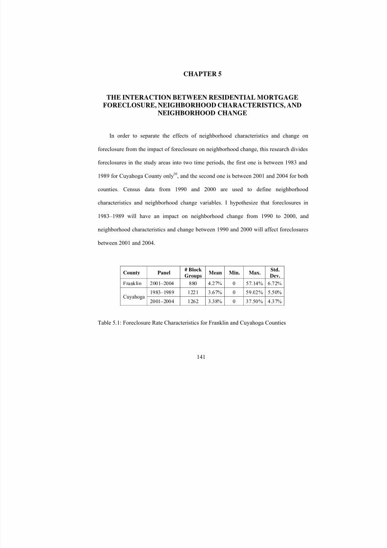
8/6/2019 Spatial Lag Regression
http://slidepdf.com/reader/full/spatial-lag-regression 155/268
8/6/2019 Spatial Lag Regression
http://slidepdf.com/reader/full/spatial-lag-regression 156/268
142
In Franklin County in 2001–2004 the aggregated average foreclosure rate is 4.27%,
with a maximum of 57.14% and a standard deviation of 6.72% (see Table 5.1).
Cuyahoga County’s foreclosure rate is lower in this time period, with an aggregated
average foreclosure rate of 3.38%. The highest rate is 37.50%. In 1983–1989 the
aggregated average foreclosure rate is 3.67% and the highest rate is 59.02%. Since the
two time periods do not have the same length, those numbers are not precisely
comparable.. Compared to Franklin County, the distribution of foreclosures in Cuyahoga
County is more even, especially in the data period (both 1983–1989 and 2001–2004)
according to the standard deviation. There is a larger percent of block groups that have
been affected by foreclosures (see Table 5.1).
Table 5.2 includes the basic descriptive statistics for all the variables used in this
analysis of the interactive mutual relationships between foreclosures, neighborhood
characteristics, and neighborhood change for Franklin County and Cuyahoga County. We
notice that most of the variables are significantly different between the two counties
(including the foreclosure rates in 2001–2004). In the next sections, we will undertake:
1. Several different regressions to estimate the neighborhood effects on foreclosures
using the 2001–2004 foreclosure rates in each county. These models include OLS, spatial
models and using H-Robust OLS for heteroskedasticity correction. We will run the
models separately for each county. 2. Seemingly Unrelated Regression (SUR) to estimate
the impact of foreclosures on neighborhood change using the 1983–1989 foreclosure
rates in Cuyahoga County only since the comparable data in Franklin County are not
available.
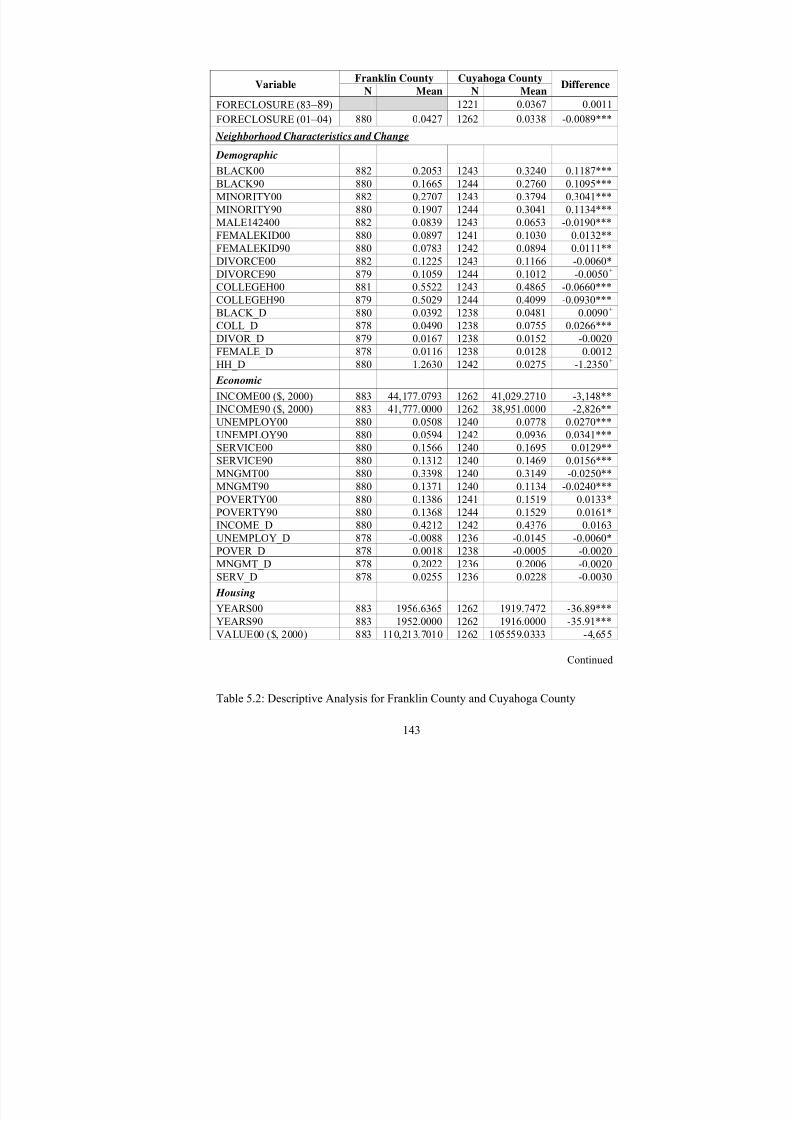
8/6/2019 Spatial Lag Regression
http://slidepdf.com/reader/full/spatial-lag-regression 157/268
143
Franklin County Cuyahoga CountyVariable
N Mean N MeanDifference
FORECLOSURE (83 –89) 1221 0.0367 0.0011
FORECLOSURE (01 – 04) 880 0.0427 1262 0.0338 -0.0089***
Neighborhood Characteristics and Change
Demographic
BLACK00 882 0.2053 1243 0.3240 0.1187***
BLACK90 880 0.1665 1244 0.2760 0.1095***
MINORITY00 882 0.2707 1243 0.3794 0.3041***
MINORITY90 880 0.1907 1244 0.3041 0.1134***
MALE142400 882 0.0839 1243 0.0653 -0.0190***
FEMALEKID00 880 0.0897 1241 0.1030 0.0132**
FEMALEKID90 880 0.0783 1242 0.0894 0.0111**
DIVORCE00 882 0.1225 1243 0.1166 -0.0060*
DIVORCE90 879 0.1059 1244 0.1012 -0.0050+
COLLEGEH00 881 0.5522 1243 0.4865 -0.0660***
COLLEGEH90 879 0.5029 1244 0.4099 -0.0930***BLACK_D 880 0.0392 1238 0.0481 0.0090+
COLL_D 878 0.0490 1238 0.0755 0.0266***
DIVOR_D 879 0.0167 1238 0.0152 -0.0020
FEMALE_D 878 0.0116 1238 0.0128 0.0012
HH_D 880 1.2630 1242 0.0275 -1.2350+
Economic
INCOME00 ($, 2000) 883 44,177.0793 1262 41,029.2710 -3,148**
INCOME90 ($, 2000) 883 41,777.0000 1262 38,951.0000 -2,826**
UNEMPLOY00 880 0.0508 1240 0.0778 0.0270***
UNEMPLOY90 880 0.0594 1242 0.0936 0.0341***
SERVICE00 880 0.1566 1240 0.1695 0.0129**
SERVICE90 880 0.1312 1240 0.1469 0.0156***
MNGMT00 880 0.3398 1240 0.3149 -0.0250**
MNGMT90 880 0.1371 1240 0.1134 -0.0240***
POVERTY00 880 0.1386 1241 0.1519 0.0133*
POVERTY90 880 0.1368 1244 0.1529 0.0161*
INCOME_D 880 0.4212 1242 0.4376 0.0163
UNEMPLOY_D 878 -0.0088 1236 -0.0145 -0.0060*
POVER_D 878 0.0018 1238 -0.0005 -0.0020
MNGMT_D 878 0.2022 1236 0.2006 -0.0020
SERV_D 878 0.0255 1236 0.0228 -0.0030
Housing
YEARS00 883 1956.6365 1262 1919.7472 -36.89***YEARS90 883 1952.0000 1262 1916.0000 -35.91***
VALUE00 ($, 2000) 883 110,213.7010 1262 105559.0333 -4,655
Continued
Table 5.2: Descriptive Analysis for Franklin County and Cuyahoga County
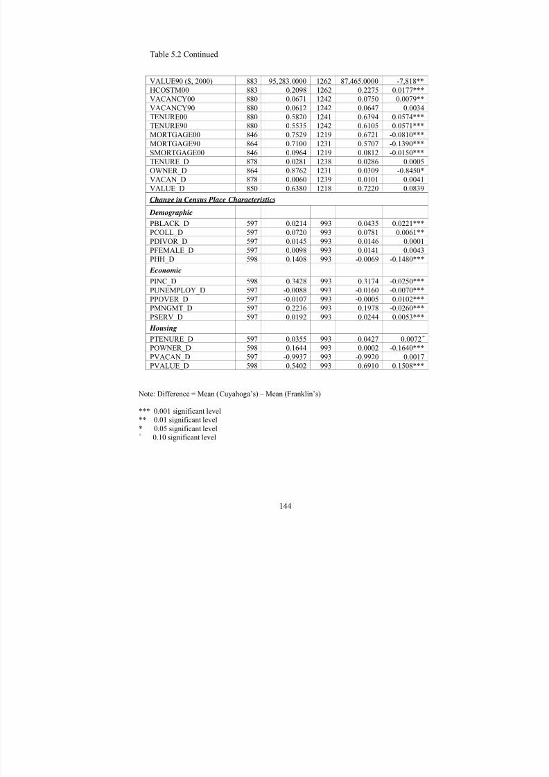
8/6/2019 Spatial Lag Regression
http://slidepdf.com/reader/full/spatial-lag-regression 158/268
144
Table 5.2 Continued
VALUE90 ($, 2000) 883 95,283.0000 1262 87,465.0000 -7,818**
HCOSTM00 883 0.2098 1262 0.2275 0.0177***
VACANCY00 880 0.0671 1242 0.0750 0.0079**
VACANCY90 880 0.0612 1242 0.0647 0.0034
TENURE00 880 0.5820 1241 0.6394 0.0574***
TENURE90 880 0.5535 1242 0.6105 0.0571***
MORTGAGE00 846 0.7529 1219 0.6721 -0.0810***
MORTGAGE90 864 0.7100 1231 0.5707 -0.1390***
SMORTGAGE00 846 0.0964 1219 0.0812 -0.0150***
TENURE_D 878 0.0281 1238 0.0286 0.0005
OWNER_D 864 0.8762 1231 0.0309 -0.8450*
VACAN_D 878 0.0060 1239 0.0101 0.0041
VALUE_D 850 0.6380 1218 0.7220 0.0839
Change in Census Place Characteristics
Demographic
PBLACK_D 597 0.0214 993 0.0435 0.0221***
PCOLL_D 597 0.0720 993 0.0781 0.0061**
PDIVOR_D 597 0.0145 993 0.0146 0.0001
PFEMALE_D 597 0.0098 993 0.0141 0.0043
PHH_D 598 0.1408 993 -0.0069 -0.1480***
Economic
PINC_D 598 0.3428 993 0.3174 -0.0250***
PUNEMPLOY_D 597 -0.0088 993 -0.0160 -0.0070***
PPOVER_D 597 -0.0107 993 -0.0005 0.0102***
PMNGMT_D 597 0.2236 993 0.1978 -0.0260***
PSERV_D 597 0.0192 993 0.0244 0.0053***
Housing
PTENURE_D 597 0.0355 993 0.0427 0.0072+
POWNER_D 598 0.1644 993 0.0002 -0.1640***
PVACAN_D 597 -0.9937 993 -0.9920 0.0017
PVALUE_D 598 0.5402 993 0.6910 0.1508***
Note: Difference = Mean (Cuyahoga’s) – Mean (Franklin’s)
*** 0.001 significant level
** 0.01 significant level* 0.05 significant level+ 0.10 significant level

8/6/2019 Spatial Lag Regression
http://slidepdf.com/reader/full/spatial-lag-regression 159/268
145
The following sections will present the research results for the research questions
about the effect of neighborhoods on foreclosures and the impact of foreclosures on
neighborhoods separately. We begin with the comparison between OLS regressions,
spatial regressions and heterscedasticity-corrected regressions to compare the model
results and develop the best prediction of the effect of neighborhoods characteristics on
foreclosure rates. SUR is used to explore how foreclosures contribute to neighborhood
change.
Effects of Neighborhoods on Foreclosure
In order to explore how neighborhood indicators and change affect foreclosure rates
in different block groups the three sets of variables (demographic, economic and housing
characteristics) and the changes in the variables are used in the analysis. For the
foreclosure panel data from 2001 to 2004 static neighborhood characteristics are
measured by the 2000 census block group values. In these models only the variables at
the neighborhood level are used. The demographic characteristics and changes include
indicators of racial composition, family structure, educational attainment, and percentage
divorced population. The effects of percent black population and percent minority
population are separately considered in the model because the two effects might be
different. The economic characteristics and changes include variables related to median
household income, unemployment rate, occupational structure and percentage population
below the poverty line. Housing characteristics and change variables include the median
years that the housing units were built (e.g., 19xx), median housing value of owner-
occupied housing units, average housing cost burden, housing vacancy rate,
8/6/2019 Spatial Lag Regression
http://slidepdf.com/reader/full/spatial-lag-regression 160/268
146
homeownership rate, and the mortgage status of owner-occupied housing units. Please
refer to the previous section and Chapter 3 for detailed narratives and statistical
descriptions of the selected variables.
As mentioned in Chapter 3, since spatial data are used in the research the effect of
spatial autocorrelation should be tested as the first step of the analysis. Ordinary Least
Square (OLS) methods were used in Geoda to test the spatial dependency of the model.
Then if there are significant spatial autocorrelation effects in the OLS model, spatial lag
or error models have to be tested to see how the spatial autocorrelation has affected the
model results. Originally only the neighborhood change variables are included in the
OLS model to predict foreclosure rates and the effect of spatial autocorrelation. This
research finds that spatial models have significantly improved the model fit by increasing
the log likelihood. When static neighborhood characteristics are added into the model the
effect of spatial autocorrelation still exists, but the effects have been reduced
significantly. This means that spatial autocorrelation is more significant when not
controlling for static neighborhood characteristics.
When combining the two counties and adding a dummy variable standing for each
county I found that the two counties are significantly different in terms of neighborhood
effects on foreclosures. Therefore each county will be separated to run the regression
models to see how the effects differ.
After running the OLS model I found that heteroskedasticity is significant for both
counties. In this situation I used White’s robust standard errors to correct for
heteroskedasticity. Then I compared the results with the spatial models. Thus I will report
results from an OLS model, a model corrected for spatial autocorrelation and a model
8/6/2019 Spatial Lag Regression
http://slidepdf.com/reader/full/spatial-lag-regression 161/268
147
corrected for heteroskedasticity. At present I am unable to correct for both spatial
autocorrelation and heterscedasticity in the same model. Thus I will focus my analysis
only on the variables that are significant in both the Heteroskedasticity-Robust OLS11
models and the Spatial Models. There is no difference in the coefficients, but there is a
difference in the levels of significance. Thus to make the analysis as conservative as
possible, the significance levels of the variables analyzed are determined based on
whichever model has the lower significance level for a specific variable . In this way I
hope to correct for both heteroskedasticity and spatial autocorrelation even though I am
unable to run a statistical model that simultaneously corrects both. Since this method
corrects for both heteroskedasticity and spatial autocorrelation separately, future work
should formally correct for heteroskedasticity and spatial autocorrelation at the same
time.
Summary of OLS and Spatial Regression Models
The OLS results of Franklin County’s neighborhood effects on foreclosures indicate
that the R 2 is 0.55, which means a relatively good fit. The Jarque-Bera test is used to
check for multicollinearity and the result is significant, which indicates that the R-square
might improve if multicollinearity is reduced. However, the variables were included for
sound theoretical reasons so the research will continue to use them all. Heteroskedasticity
is significant for the model too, which means that the error term does not have a constant
variance and thus the significant heteroskedasticity has violated one assumption of OLS..
Also the variance of the coefficient distribution increases. However, it is usually difficult
to determine the nature of the bias. But the significant heteroskedasticity will not yield

8/6/2019 Spatial Lag Regression
http://slidepdf.com/reader/full/spatial-lag-regression 162/268
148
biased coefficient estimates. The issue of significant heteroskedasticity can be corrected
or alleviated by redefining the variables, using Weighted Least Squares to re-estimate the
equation, or when working with large samples, using heteroskedasticity-corrected errors
to make the standard errors more accurate (though still biased).
All the indicators of spatial dependence are significant. In this situation both spatial
error and spatial lag models are used to see which one will have the best fit. We notice
(see Table 5.3) that both models have improved the R-square slightly12. The spatial lag
model turns out to have the higher R 2
(0.60) and the spatial lag term is highly significant,
although heteroskedasticity still exists. Among the three models (OLS, spatial error and
spatial lag) the spatial lag model also has the highest log likelihood. Because it is the
strongest model the parameter estimates from the spatial lag model will be analyzed to
see what neighborhood characteristics and changes significantly affect the foreclosure
rates in Franklin County.
Notice that the R 2
is 0.54 for the OLS model for Cuyahoga County (see Table 5.4).
Muticollinearity and Heteroskedasticity are apparent in this regression as they were for
Franklin County. Like Franklin County, when only the change variables are included the
effect of spatial autocorrelation on the foreclosure rates is large. But when the static
neighborhood characteristic variables are added the spatial effect is greatly reduced. All
the indicators for diagnosing spatial dependence (LM lag, Robust LM lag, LM error, and
Robust LM error) are significant. Again, both the spatial error and lag models are tested
to see which one has the best fit. The spatial lag model has the highest log likelihood in
Cuyahoga County as it did in Franklin County. Therefore the spatial lag model is the best
fit, although the three models (OLS, spatial error and spatial lag) yield very similar

8/6/2019 Spatial Lag Regression
http://slidepdf.com/reader/full/spatial-lag-regression 163/268
149
results (as they did in Franklin County). Notice that change in the homeownership rate
does not affect foreclosure rates in the OLS model while it does in the Spatial Lag Model
(see Table 5.4). This is important because when the spatial autocorrelation of foreclosures
is controlled the homeownership rate is significantly related to foreclosure rates. Thus
considering spatial effects can improve the model results by changing our view of the
neighborhood effects on foreclosures. But the most important reason for using the spatial
models is because they can yield more efficient estimates by accounting for spatial
effects and the effects of related omitted variables.
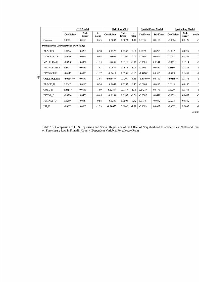
8/6/2019 Spatial Lag Regression
http://slidepdf.com/reader/full/spatial-lag-regression 164/268
1
5 0
OLS Model H-Robust OLS Spatial Error Model
CoefficientStd-
Error
t-
ValueCoefficient
Std-
Error
t-
valueCoefficient Std-Error
Constant 0.0082 0.0191 0.43 0.0082 0.0073 1.12 0.0136 0.0188
Demographic Characteristics and Change
BLACK00 0.0276 0.0283 0.98 0.0276 0.0345 0.80 0.0277 0.0293
MINORITY00 -0.0010 0.0265 -0.04 -0.001 0.0290 -0.03 0.0090 0.0271
MALE142400 -0.0390 0.0338 -1.15 -0.039 0.0511 -0.76 -0.0305 0.0341
FEMALEKID00 0.0677+ 0.0350 1.93 0.0677 0.0646 1.05 0.0502 0.0350
DIVORCE00 -0.0617 0.0525 -1.17 -0.0617 0.0708 -0.87 -0.0920+ 0.0516
COLLEGEH00 -0.0664*** 0.0183 -3.64 -0.0664** 0.0201 -3.31 -0.0740*** 0.0182
BLACK_D 0.0047 0.0197 0.24 0.0047 0.0282 0.17 -0.0009 0.0197
COLL_D 0.0357* 0.0180 1.99 0.0357+ 0.0187 1.91 0.0435* 0.0176
DIVOR_D -0.0284 0.0433 -0.65 -0.0284 0.0505 -0.56 -0.0307 0.0418
FEMALE_D 0.0209 0.0357 0.58 0.0209 0.0503 0.42 0.0155 0.0342
HH_D -0.0003 0.0002 -1.23 -0.0003+ 0.0002 -1.91 -0.0003 0.0002
Table 5.3: Comparison of OLS Regression and Spatial Regression of the Effect of Neighborhood Charon Foreclosure Rate in Franklin County (Dependent Variable: Foreclosure Rate)

8/6/2019 Spatial Lag Regression
http://slidepdf.com/reader/full/spatial-lag-regression 165/268
1
5 1
Table 5.3 Continued
Economic Characteristics and Change
INCOME00 5.09E-007* 2.02E-007 2.525.09E-
07**
1.7759E-07
2.874.01E-
007*2.01E-007
UNEMPLOY00 0.1408** 0.0519 2.71 0.1408 0.1242 1.13 0.1307** 0.0495
SERVICE00 0.1229** 0.0412 2.98 0.1229+ 0.0663 1.85 0.0956* 0.0396
MNGMT00 -0.0038 0.0353 -0.11 -0.0038 0.0340 -0.11 -0.0170 0.0341
POVERTY00 0.0604* 0.0235 2.57 0.0604+ 0.0310 1.95 0.0262 0.0235
INCOME_D 0.0080 0.0049 1.63 0.008 0.0070 1.14 0.0104* 0.0046
UNEMPLOY_D -0.0221 0.0393 -0.56 -0.0221 0.0751 -0.29 -0.0063 0.0373
POVER_D -0.0655** 0.0252 -2.60 -0.0655* 0.0282 -2.32 -0.0372 0.0241
MNGMT_D 0.0053 0.0302 0.18 0.0053 0.0291 0.18 -0.0023 0.0294
SERV_D -0.0438 0.0331 -1.32 -0.0438 0.0469 -0.93 -0.0304 0.0314
Housing Characteristics and Change
YEARS00 -2.77E-005* 1.30E-005 -2.12 -2.77E-05*
1.1963E-
05 -2.32 -1.26E-005 1.29E-005
VALUE00 -1.02E-007* 5.10E-008 -2.00 -1.02E-07*4.9611E-
08-2.06 -5.18E-008 0

8/6/2019 Spatial Lag Regression
http://slidepdf.com/reader/full/spatial-lag-regression 166/268
1
5 2
Table 5.3 Continued
HCOSTM00 0.0011*** 0.0003 3.79 0.0011* 0.0004 2.47 0.0011*** 0.0003
VACANCY00 0.3375*** 0.0474 7.13 0.3375*** 0.0710 4.75 0.2708*** 0.0474
TENURE00 0.0286* 0.0124 2.31 0.0286* 0.0139 2.05 0.0182 0.0122
MORTGAGE00 0.0188+ 0.0097 1.95 0.0188 0.0148 1.27 0.0114 0.0094
SMORTGAGE000.0315+ 0.0190 1.65 0.0315 0.0310 1.02 0.0357* 0.0178
TENURE_D -0.0944*** 0.0166 -5.69 -0.0944** 0.0297 -3.18 -0.0894*** 0.0158
OWNER_D 0.0005 0.0005 0.95 0.0005 0.0003 1.44 0.0006 0.0005
VACAN_D -0.2132*** 0.0465 -4.58 -0.2132*** 0.0623 -3.42 -0.1610*** 0.0458
VALUE_D -0.0019* 0.0008 -2.56 -0.0019** 0.0007 -2.60 -0.0013+ 0.0007
LAMDA 0.3522*** 0.0457
W-FORECLOSURE
# of Observations 883 883
R-Square 0.55 0.58
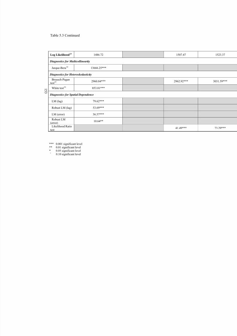
8/6/2019 Spatial Lag Regression
http://slidepdf.com/reader/full/spatial-lag-regression 167/268
1
5 3
Table 5.3 Continued
Log Likelihood13 1486.72 1507.47
Diagnostics for Multicollinearity
Jarque-Bera14 13666.25***
Diagnostics for Heteroskedasticity
Breusch-Pagantest15
2960.84*** 2962.92***
White test16 853.01***
Diagnostics for Spatial Dependence
LM (lag) 79.62***
Robust LM (lag) 53.69***
LM (error) 36.57***
Robust LM(error)
10.64**
Likelihood Ratiotest
41.49***
*** 0.001 significant level** 0.01 significant level* 0.05 significant level+ 0.10 significant level

8/6/2019 Spatial Lag Regression
http://slidepdf.com/reader/full/spatial-lag-regression 168/268
1
5 4
OLS Model H-Robust OLS Spatial Error Model
CoefficientStd-
Error
t-
valueCoefficient
Std-
Error
t-
valueCoefficient Std-Error
Constant 0.0005 0.0067 0.07 0.0005 0.0011 0.44 0.0123+ 0.0071
Demographic Characteristics and Change
BLACK00 0.0289* 0.0130 2.22 0.0289+ 0.0152 1.91 0.0212 0.0143
MINORITY00 0.0067 0.0139 0.48 0.0067 0.0160 0.42 0.0203 0.0150
MALE142400 0.0281 0.0250 1.13 0.0281 0.0425 0.66 0.0246 0.0237
FEMALEKID00 0.0456** 0.0170 2.69 0.0456 0.0392 1.16 0.0392* 0.0164
DIVORCE00 -0.0200 0.0253 -0.79 -0.02 0.0344 -0.58 -0.0110 0.0243
COLLEGEH00 -0.0267* 0.0115 -2.32 -0.0267* 0.0114 -2.34 -0.0281* 0.0115
BLACK_D 0.0203* 0.0085 2.40 0.0203* 0.0103 1.97 0.0182+ 0.0095
COLL_D 0.0079 0.0109 0.73 0.0079 0.0132 0.60 0.0101 0.0105
DIVOR_D 0.0204 0.0200 1.02 0.0204 0.0262 0.78 0.0097 0.0191
FEMALE_D -0.0054 0.0175 -0.31 -0.0054 0.0345 -0.16 -0.0040 0.0167
HH_D 0.0013 0.0019 0.68 0.0013 0.0026 0.49 0.0006 0.0018
Table 5.4: Comparison of OLS Regression and Spatial Regression of the Effect of Neighborhood Charon Foreclosure Rate in Cuyahoga County (Dependent Variable: Foreclosure Rate)

8/6/2019 Spatial Lag Regression
http://slidepdf.com/reader/full/spatial-lag-regression 169/268
1
5 5
Table 5.4 Continued
Economic Characteristics and Change
INCOME00 3.52E-7*** 1.06E-7 3.313.52E-
07***
9.9591E-08
3.53 2.92E-7** 1.04E-7
UNEMPLOY00 -0.0176 0.0249 -0.71 -0.0176 0.0421 -0.42 -0.0126 0.0237
SERVICE00 -0.0108 0.0177 -0.61 -0.0108 0.0293 -0.37 -0.0228 0.0172
MNGMT00 -0.0305 0.0207 -1.47 -0.0305 0.0251 -1.22 -0.0204 0.0199
POVERTY00 0.0557*** 0.0154 3.61 0.0557* 0.0263 2.11 0.0374* 0.0152
INCOME_D -0.0016 0.0023 -0.69 -0.0016 0.0033 -0.49 -0.0020 0.0022
UNEMPLOY_D 0.0183 0.0167 1.09 0.0183 0.0346 0.53 0.0216 0.0159
POVER_D -0.0368** 0.0139 -2.64 -0.0368+ 0.0211 -1.74 -0.0341* 0.0135
MNGMT_D 0.0023 0.0171 0.14 0.0023 0.0191 0.12 -0.0066 0.0165
SERV_D -0.0115 0.0137 -0.84 -0.0115 0.0209 -0.55 -0.0039 0.0132
Housing Characteristics and Change
YEARS00 2.31E-006 5.82E-006 0.39 2.31E-06
8.6598E-
06 0.27 2.05E-006 5.95E-006
VALUE00 -4.16E-008 2.77E-008 -1.50 -4.16E-082.7978E-
08-1.49 -3.68E-008 0

8/6/2019 Spatial Lag Regression
http://slidepdf.com/reader/full/spatial-lag-regression 170/268
1
5 6
Table 5.4 Continued
HCOSTM00 0.0587*** 0.0132 4.44 0.0587* 0.0243 2.42 0.0381** 0.0128
VACANCY00 0.0466* 0.0228 2.05 0.0466 0.0482 0.97 0.0546* 0.0221
TENURE00 -0.0163* 0.0068 -2.40 -0.0163+ 0.0086 -1.88 -0.0117+ 0.0068
MORTGAGE000.0181** 0.0063 2.89 0.0181+ 0.0107 1.70 0.0057 0.0061
SMORTGAGE00-0.0129 0.0124 -1.04 -0.0129 0.0158 -0.82 -0.0001 0.0120
TENURE_D -0.0211 0.0131 -1.62 -0.0211 0.0162 -1.30 -0.0343** 0.0123
OWNER_D -0.0117*** 0.0033 -3.54 -0.0117+ 0.0066 -1.77 -0.0086** 0.0031
VACAN_D 0.0287 0.0200 1.43 0.0287 0.0430 0.67 0.0163 0.0195
VALUE_D 0.0033* 0.0013 2.48 0.0033 0.0028 1.18 0.0036** 0.0013
LAMDA 0.3535*** 0.0384
W-FORECLOSURE
# of Observations 1262 1262
R-Square 0.54 0.58
Log Likelihood17 2657.05 2686.90
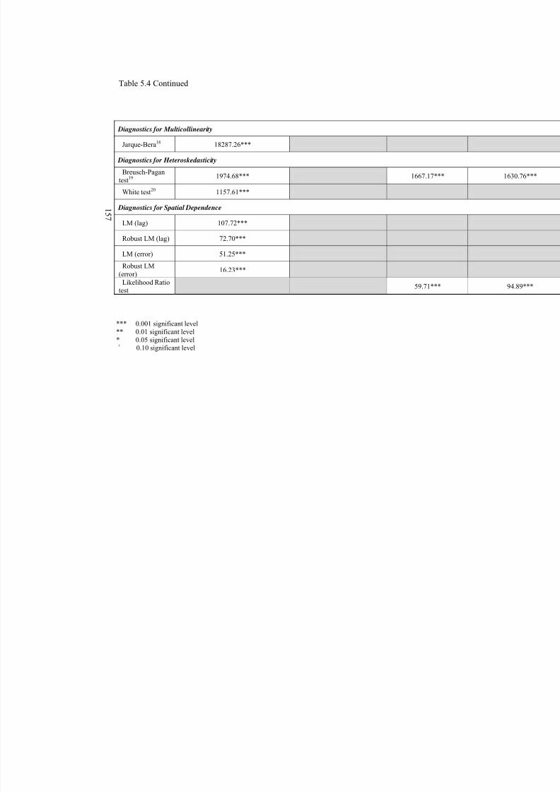
8/6/2019 Spatial Lag Regression
http://slidepdf.com/reader/full/spatial-lag-regression 171/268
1
5 7
Table 5.4 Continued
Diagnostics for Multicollinearity
Jarque-Bera18 18287.26***
Diagnostics for Heteroskedasticity
Breusch-Pagantest19
1974.68*** 1667.17***
White test20 1157.61***
Diagnostics for Spatial Dependence
LM (lag) 107.72***
Robust LM (lag) 72.70***
LM (error) 51.25***
Robust LM(error)
16.23***
Likelihood Ratiotest
59.71***
*** 0.001 significant level** 0.01 significant level* 0.05 significant level+ 0.10 significant level

8/6/2019 Spatial Lag Regression
http://slidepdf.com/reader/full/spatial-lag-regression 172/268
158
The following narrative will report the variables that are significant for both the
Heteroskedasticity-Robust OLS and Spatial Lag Model, so that we can make the results
more efficient by correcting for each problem separately but considering their results
together.
In Franklin County, when the Robust OLS model and the spatial lag models are both
used none of the change variables among the demographic characteristics are significant.
However, one static neighborhood characteristic is significant in both models and thus is
related to foreclosures (see Table 5.3).
In addition racial composition in 2000, which was assumed to affect foreclosures, is
not significant for Franklin County, when controlling for other factors. The percentage
divorced population does not affect foreclosures either. The only one demographic
variable that is significant is percentage population with college degree or higher and the
relationship, as expected, is negative.
None of the economic change variables have an effect on foreclosure rates in
Franklin County. Median household income in 2000 has a positive relationship with
foreclosures in both models. This seems strange since higher income should be associated
with lower foreclosure rates. Perhaps this is the remaining effect of median income once
educational level is accounted for. Poverty level and percentage population employed in
executive or management occupation do not have a significant impact on foreclosure
rates. However, percentage population employed in service occupations is significant and
positive in both of the models we are considering.
More changes in housing characteristics have significant impacts on foreclosure
rates in neighborhoods in Franklin County than any other variable type. Change in the
8/6/2019 Spatial Lag Regression
http://slidepdf.com/reader/full/spatial-lag-regression 173/268
159
homeownership rate, change in the housing vacancy rate, and change in housing value
are all negatively related to foreclosure rates. This means that high turnover and change
in housing characteristics in 1990–2000 are related to foreclosure rates in 2001–2004 in
Franklin County. The change in housing vacancy rates is negatively related to
foreclosures and this might mean that more dynamic housing markets have fewer
foreclosures. Among static housing characteristics in 2000 the average housing cost
burden and the housing vacancy rate are significant factors affecting foreclosure rates and
both are positive in both the H-Robust model and the spatial lag model. Thus
neighborhoods where residents pay significant portions of their income, and those with
high vacancy rates are at more risk of foreclosures in Franklin County.
In Cuyahoga County, the effect of neighborhood demographic characteristics and
change on foreclosure is very similar to that in Franklin County. Educational attainment
in 2000 is the one of the major factors in both equations, with the expected negative sign.
But in Cuyahoga County percentage black population and its change are also significant
(and positive) in affecting foreclosures, although the significance level is 0.10. The
potential reason for this difference between the two counties might be the difference in
racial composition between the two counties. Cuyahoga County has a larger percent of
black population than Franklin County. So either the larger proportion or more
segregation could cause this effect. The standard deviation of percentage black
population is larger than that in Franklin County too, which means that black population
in Cuyahoga County is more clustered than in Franklin County. Percentage minority
population does not have a significant effect on foreclosures in either county.
8/6/2019 Spatial Lag Regression
http://slidepdf.com/reader/full/spatial-lag-regression 174/268
160
Cuyahoga County’s results for the impact of economic neighborhood characteristics
on foreclosure rates are slightly different from those for Franklin County. The percentage
population below the poverty line (positive) and its change (negative) has significant
impacts on foreclosures in Cuyahoga County unlike Franklin County. Similar to Franklin
County, median household income has a positive relationship with foreclosures. The
change in percentage population below the poverty line is negatively related to
foreclosures and this might be because of collinearity, omitted variables, and some other
reasons. While in Franklin County, occupational structure (percentage population
employed in service occupations) also affects foreclosures, but this has no significant
impact in Cuyahoga County.
Average housing cost burden, Homeownership rate, change in number of owner-
occupied housing units, and percentage of housing units with a mortgage are all
significant factors affecting foreclosures in Cuyahoga County in both models. This is
very different from Franklin County. In fact, average housing cost burden is the only
common factor for both counties regarding the effect of housing characteristics and
change on foreclosures.
Common Neighborhood Characteristics Affecting Foreclosures in Both Counties
Educational Attainment
The importance of residents’ educational attainment in determining neighborhood
quality has been stated in previous chapters. Educational attainment is highly related to
median household income, housing value, and other neighborhood or personal indicators.
But when controlling for most of those indicators educational attainment still remains
8/6/2019 Spatial Lag Regression
http://slidepdf.com/reader/full/spatial-lag-regression 175/268
161
significant. This might mean that educational attainment is more important than other
factors in contributing to foreclosure. Another explanation of why educational attainment
in a neighborhood is related to foreclosure might be because the higher the educational
attainment of a household the more possible it is for them to have a prime loan. They will
also be less likely to become the victims of predatory lending. The models found that the
higher the educational attainment of the residents in a neighborhood the lower the
foreclosure rate in that neighborhood for both counties, controlling for other factors.
Median Household Income
We expected that median household income will be negatively related to
foreclosures. But this research finds that in both counties median household income is
positively related to foreclosure rates. This seems strange. But this might be because
although a neighborhood has a higher income the housing cost burden can be high, thus
contributing to more foreclosures. As suggested above, this may be a residual effect after
educational attainment is taken into account. Another explanation is that householders
with lower income in a higher income neighborhood might be more likely to default on
their properties and thus increased the foreclosure rates in that neighborhood. However,
those explanations should not ignore the possible effect of omitted variables and other
factors in the regression.
Average Housing Cost Burden
The average housing cost burden is measured by the ratio of housing expenses (with
a mortgage) to monthly income in the neighborhood. The results indicate that a higher
8/6/2019 Spatial Lag Regression
http://slidepdf.com/reader/full/spatial-lag-regression 176/268
162
housing cost burden has a positive effect on foreclosure rates. In the spatial lag model in
Franklin County a one percentage point increase (or decrease) in the average housing cost
burden is related to a foreclosure rate increase (or decrease) of 0.0011% points. This
effect is not very large but it is significant at the 0.001 level (see Table 5.3). In Cuyahoga
County when the housing cost burden is 1% point higher (or lower) foreclosure rates
increase (or decrease) by 0.0391% points (see Table 5.4). This result is consistent with
that in Franklin County. A large housing cost burden seems to be a consistent indicator
of neighborhoods with higher foreclosure risks.
Difference in the Effect of Neighborhood Characteristics on Foreclosures in Each
County
Franklin County
Percentage Labor Force Employed in Service Occupation
The use of the variable percentage labor force employed in service occupations in
this research is intended to explore how service occupations, which are often associated
with lower paying and/or unstable jobs, affect foreclosure rates in neighborhoods. The
results in Franklin County indicate that service employment is positively related to
foreclosure rates. The variable was not significant in Cuyahoga County.
Housing Vacancy Rate
The housing vacancy rate is one of the most important indicators of the health of
housing markets. Higher housing vacancy rates usually mean a surplus of housing supply
compared to housing demand. Housing vacancy is necessary in the housing market since
in many situations the housing absorption rate cannot be as high as 100% (if it were
8/6/2019 Spatial Lag Regression
http://slidepdf.com/reader/full/spatial-lag-regression 177/268
163
mobility would be severely restricted). A moderate to low housing vacancy rate usually
will not have a significant negative effect on the housing markets (thought it might drive
up prices). But a high housing vacancy rate indicates a housing market that is unhealthy.
This research found that the housing vacancy rate has a significant positive impact on the
foreclosure rate in one of the two study areas, but not the other. This means that
neighborhoods with a weak housing market will have much higher foreclosure rates.
Change in Homeownership Rate
The homeownership rate in a neighborhood should be related to foreclosures
because previous research found that homeownership is highly related to neighborhood
quality and stability. We find that the change in the homeownership rate is negatively
related to foreclosures in Franklin County only (see Table 5.3). This means that increases
in the homeownership rate will lower the foreclosure rate in a neighborhood in that
county.
Change in Housing Vacancy Rate
The research results indicate that the higher the change in housing vacancy rate in a
neighborhood, the lower the foreclosure rates in Franklin County. This means that the
increases in vacancy rates in a neighborhood are negatively related to foreclosure rates.
This seems counter intuitive, but might indicate that the more dynamic a neighborhood
housing market is the less likely the neighborhood will have a high foreclosure rate.
8/6/2019 Spatial Lag Regression
http://slidepdf.com/reader/full/spatial-lag-regression 178/268
164
Change in Median Housing Value
In the literature housing value is found to have a strong impact on foreclosures,
especially for individual homeowners. Many scholars believe that negative home equity
is one of the factors leading to mortgage default decisions of the borrowers and it can
arise from negative appreciation and low house values. However this study examines
neighborhoods, not individual owners and found that the median housing value does not
have an effect on foreclosure rates at the neighborhood level, holding other things
constant. However, in Franklin County the change in median housing value has a
negative relationship with foreclosure rate. When the average housing values increase
foreclosure rates decrease. This argues that change in value is more critical than the
average value in a neighborhood in Franklin County and an upward trajectory is
important as we would expect.
Cuyahoga County
Percentage Black Population and Change
We found that racial composition and turnover (especially percentage black
population and change in percentage black population) have a significant positive impact
on foreclosures in Cuyahoga County. The more racial turnover (i.e. increase in
percentage black population), the higher the foreclosure rate, which means that racially
stable neighborhoods will have a relatively lower foreclosure rate, though stable white
neighborhoods have lower foreclosure rates than stable black neighborhoods.
8/6/2019 Spatial Lag Regression
http://slidepdf.com/reader/full/spatial-lag-regression 179/268
165
Percentage Population below the Poverty Line and Change
Percentage population below the poverty line has a positive impact on foreclosures
in Cuyahoga County. Therefore, poorer neighborhoods are often associated with higher
foreclosure rates in Cuyahoga County, but not in Franklin County.
A higher poverty level in 2000 is associated with higher foreclosure rates in the later
time period, but the more the poverty rate increased between 1990 and 2000, the smaller
that effect. This might mean that when there is more population below the poverty line,
housing affordability will decrease thus fewer people will have mortgages. Foreclosure
rates will decrease with the decrease in affordability.
Homeownership Rate and Change in Percentage Owner-occupied Housing Units
The homeownership rate has a negative relationship with foreclosure rates. This
result is different from that in Franklin County because in Franklin County the
homeownership rate itself does not have an impact on foreclosures. The change in
percentage owner-occupied housing units is also found to be positively related to
foreclosure rates in Cuyahoga County. The effect is similar to that of the change in
homeownership rate.
Percentage Housing Units with a Mortgage
This indicator has a significant effect on foreclosures in Cuyahoga County but not in
Franklin County. The larger the percentage owner-occupied housing units with a
mortgage, the higher the foreclosure rates (see Table 5.4). In contemporary U.S. society
the majority of owner households hold a mortgage. In Franklin County the

8/6/2019 Spatial Lag Regression
http://slidepdf.com/reader/full/spatial-lag-regression 180/268

8/6/2019 Spatial Lag Regression
http://slidepdf.com/reader/full/spatial-lag-regression 181/268
167
Summary: Effects of Neighborhood Characteristics on Residential Mortgage
Foreclosure
Comparing the research results from the two counties we found that the same
economic characteristics and change variables do not significantly affect foreclosures
(see Table 5.5). This is consistent with our initial expectations because the economic
situations of the two counties are different, thus the neighborhood effects on foreclosures
might be different. However, the counties have some similarities in terms of the effect of
neighborhood characteristics and change, although some of the variables have different
impact on foreclosures in the two counties.
For both counties percentage population with college degrees or higher has a
negative impact on foreclosures. Therefore, educational attainment at the neighborhood
level is the common and important factor contributing to neighborhood foreclosures.
Educational attainment is related to many other factors. More education leads to higher
and more stable income, and the higher the educational attainment the less likely that the
residents will be the victims of mortgage fraud and/or predatory lending, thus lowering
the foreclosure rates.
For both counties median household income has a positive impact on foreclosures,
which is difficult to explain. However, this might be related to the increasing housing
cost burden. The increase in housing value and costs associated with owning a home is
much larger than the increase in median household income, thus the increase in median
household income is positively related to foreclosures. At the same time the increase in
median household income will also make it easier for homeowners to get mortgages in

8/6/2019 Spatial Lag Regression
http://slidepdf.com/reader/full/spatial-lag-regression 182/268
168
these neighborhoods, and people may stretch to purchase the most expensive houses thus
using mortgage types invented in the late 1990s which are more risky.
For both counties housing cost burdens has a positive impact on foreclosures. This is
consistent with our expectations and detailed narratives of the rationales can be found in
previous sections.
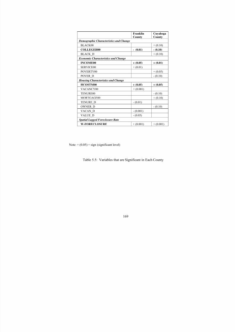
8/6/2019 Spatial Lag Regression
http://slidepdf.com/reader/full/spatial-lag-regression 183/268
169
Note: + (0.05) = sign (significant level)
Table 5.5: Variables that are Significant in Each County
Franklin
County
Cuyahoga
County
Demographic Characteristics and Change
BLACK00 + (0.10)
COLLEGEH00 - (0.01) - (0.10)
BLACK_D + (0.10)
Economic Characteristics and Change
INCOME00 + (0.05) + (0.01)
SERVICE00 + (0.01)
POVERTY00 + (0.05)
POVER_D - (0.10)
Housing Characteristics and Change
HCOSTM00 + (0.05) + (0.05)
VACANCY00 + (0.001)TENURE00 - (0.10)
MORTGAGE00 + (0.10)
TENURE_D - (0.01)
OWNER_D - (0.10)
VACAN_D - (0.001)
VALUE_D - (0.05)
Spatial Lagged Foreclosure Rate
W-FORECLOSURE + (0.001) + (0.001)

8/6/2019 Spatial Lag Regression
http://slidepdf.com/reader/full/spatial-lag-regression 184/268
170
There are some differences in neighborhood effects on foreclosures between the
two counties (see Table 5.5).
Percentage black population is related to foreclosures in Cuyahoga County but not
in Franklin County. This might be because the two counties have different racial
characteristics. In Cuyahoga County there is a larger percent of black population and the
distribution of the black population in different block groups is more segregated. Change
in percentage black population is the only change variable in demographic characteristics
that is significant for Cuyahoga County, although not for Franklin County.
Economic effects are quite different for the two counties. In Franklin County the
occupational structure has impacts on foreclosures, while in Cuyahoga County the
poverty rate (percentage population below the poverty line) and its change play dominant
roles in affecting foreclosures. It is not clear why the percentage population below the
poverty line affects foreclosures, especially when controlling for unemployment rate,
occupational structure and median household income. Probably it is because high poverty
in the neighborhood may make it unlikely that houses there will be worth anything thus
householders are more likely to walk away. The change in this percentage has a negative
relationship with foreclosure rates. This might mean that when there is a higher decrease
in percentage population below the poverty line there will be a lower foreclosure rate.
Among the housing characteristics and change variables (except average housing
cost burden), all significant variables are different between the counties. In Franklin
County, housing vacancy rates have a significant positive impact on foreclosures. This is
not surprising since higher vacancy rates are usually associated with neighborhoods with
decreased life and housing quality. The decreased housing quality will lower the housing
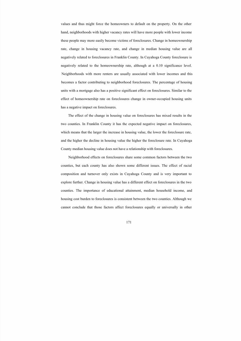
8/6/2019 Spatial Lag Regression
http://slidepdf.com/reader/full/spatial-lag-regression 185/268
171
values and thus might force the homeowners to default on the property. On the other
hand, neighborhoods with higher vacancy rates will have more people with lower income
these people may more easily become victims of foreclosures. Change in homeownership
rate, change in housing vacancy rate, and change in median housing value are all
negatively related to foreclosures in Franklin County. In Cuyahoga County foreclosure is
negatively related to the homeownership rate, although at a 0.10 significance level.
Neighborhoods with more renters are usually associated with lower incomes and this
becomes a factor contributing to neighborhood foreclosures. The percentage of housing
units with a mortgage also has a positive significant effect on foreclosures. Similar to the
effect of homeownership rate on foreclosures change in owner-occupied housing units
has a negative impact on foreclosures.
The effect of the change in housing value on foreclosures has mixed results in the
two counties. In Franklin County it has the expected negative impact on foreclosures,
which means that the larger the increase in housing value, the lower the foreclosure rate,
and the higher the decline in housing value the higher the foreclosure rate. In Cuyahoga
County median housing value does not have a relationship with foreclosures.
Neighborhood effects on foreclosures share some common factors between the two
counties, but each county has also shown some different issues. The effect of racial
composition and turnover only exists in Cuyahoga County and is very important to
explore further. Change in housing value has a different effect on foreclosures in the two
counties. The importance of educational attainment, median household income, and
housing cost burden to foreclosures is consistent between the two counties. Although we
cannot conclude that those factors affect foreclosures equally or universally in other

8/6/2019 Spatial Lag Regression
http://slidepdf.com/reader/full/spatial-lag-regression 186/268
172
counties in or out of Ohio, this research serves as a good first step in understanding the
neighborhood factors contributing to foreclosures in a neighborhood. A detailed
conclusion and policy implications based on these research results will be presented in
Chapter 6.
So far I have analyzed the effect of neighborhood characteristics and change on
foreclosure rates. In the next section I turn to the impact of foreclosure rates on
neighborhood change.
8/6/2019 Spatial Lag Regression
http://slidepdf.com/reader/full/spatial-lag-regression 187/268
173
The Impact of Residential Mortgage Foreclosure on Neighborhood Change:
A Seemingly Unrelated Regression (SUR) Approach
The impact of residential mortgage foreclosure on neighborhood change is
measured by predicting the effect of foreclosures in 1983–1989 in Cuyahoga County on
neighborhood change in 1990–2000. Since Sheriff’s Deeds in 1983–1989 in Franklin
County are not available or not geographically identifiable, only Cuyahoga County’s data
will be used to test whether mortgage foreclosure has an impact on neighborhood
changes. The results of the previous section indicate significant differences between the
two counties, so it is unfortunate that we cannot study Franklin County. However, the
research methodology can be duplicated in the future when testing the impact in other
geographic areas.
As mentioned in the research methodology section SUR systems can estimate
regression coefficients more efficiently than single-equation OLS regressions (Zellner,
1962) when certain assumptions are met. This research compares the results of OLS and
SUR, and finds that SUR can better predict the equation systems than OLS due to the
correlated cross-model errors (see Table 5.6 for the Cross Model Covariance Matrix in
Cuyahoga County) since it considers the correlation between error terms of the equations.
In SUR procedures all coefficients are estimated simultaneously by using Aitken’s
general least squares (GLS). The goodness of fit of the SUR system is generally based on
the weighted system R-square and weighted mean square error (MSE) of the equation
systems. In order to minimize the determinant of the error covariance matrix Iterated
SUR 21 (ITSUR) was used in this research. All fourteen neighborhood change variables
are used as dependent variables in the SUR system. The independent variables are chosen
based on the correlation coefficients of those variables with the change variables. The
8/6/2019 Spatial Lag Regression
http://slidepdf.com/reader/full/spatial-lag-regression 188/268
174
ones with a coefficient lower than 0.02 are omitted from the equation system. Although
independent variables in all other equations are the subsets of the ones in the equation of
median housing value (as the dependent variable), ITSUR will still be used to include the
effects of correlated error terms between equations. In ITSUR estimation, other factors,
such as spatial effects, might be omitted variables, and thus can bias the error structure.
The OLS and ITSUR estimations yield similar parameter estimates. Due to
correlated residuals between the equations, ITSUR is more efficient than OLS and
produces more accurate estimates than OLS. When running the ITSUR system, the
weighted R-square is 0.4104 and the Weighted MSE is 1.0000, with 11,276 degrees of
freedom. The model fits relatively well with the data. The results indicate that foreclosure
rates have a relationship with educational attainment, change in percentage divorced
population, change in female headship rate, change in percentage population below the
poverty line, change in homeownership rate, change in housing vacancy rate, and change
in median housing values (see Table 5.7 for details). All of the signs are consistent with
our expectations expect for the negative relationship of foreclosure rates with change in
housing vacancies and the positive relationship of foreclosures with change in property
values. Future investigations should focus on understanding these results.

8/6/2019 Spatial Lag Regression
http://slidepdf.com/reader/full/spatial-lag-regression 189/268
1 7 5
BLACK_D COLL_D DIVOR_D FEMALE_D HH_D INCOME_D
BLACK_D 0.010146 -.000391 0.000006 0.002190 -.000408 -.001299
COLL_D -.000391 0.005776 -.000051 -.000115 0.002255 0.002930
DIVOR_D 0.000006 -.000051 0.001581 0.000203 -.000645 -.000591
FEMALE_D 0.002190 -.000115 0.000203 0.003671 -.000524 -.003213
HH_D -.000408 0.002255 -.000645 -.000524 0.314843 -.000363
INCOME_D -.001299 0.002930 -.000591 -.003213 -.000363 0.071090
UNEMPLOY_D 0.000709 -.000532 -.000089 0.000598 -.001453 -.003270
POVER_D 0.001388 -.001132 0.000253 0.001468 -.001785 -.009223
MNGMT_D -.000498 0.002719 -.000080 -.000399 0.000210 0.001749
SERV_D 0.000815 -.000959 -.000016 0.000462 0.000513 -.001802
TENURE_D -.000696 0.000299 -.000344 -.001127 -.003801 0.005347
OWNER_D -.002565 0.002221 -.001085 -.001868 0.087901 0.011377
VACAN_D 0.000421 -.000193 0.000037 0.000089 -.000245 0.000171
VALUE_D -.002666 0.001252 -.001221 -.000930 0.007705 0.010164
POVER_D MNGMT_D SERV_D TENURE_D OWNER_D VACAN
BLACK_D 0.001388 -.000498 0.000815 -.000696 -.002565 0.0004
COLL_D -.001132 0.002719 -.000959 0.000299 0.002221 -.0001
DIVOR_D 0.000253 -.000080 -.000016 -.000344 -.001085 0.0000
FEMALE_D 0.001468 -.000399 0.000462 -.001127 -.001868 0.0000
Table 5.6: Cross Model Covariance Matrix for Cuyahoga County

8/6/2019 Spatial Lag Regression
http://slidepdf.com/reader/full/spatial-lag-regression 190/268
1 7 6
Table 5.6 Continued
HH_D -.001785 0.000210 0.000513 -.003801 0.087901 -.0002
INCOME_D -.009223 0.001749 -.001802 0.005347 0.011377 0.0001
UNEMPLOY 0.001122 -.000062 -.000009 -.000524 -.002604 0.0000
POVER_D 0.005798 -.000254 0.000436 -.001630 -.003185 0.0002
MNGMT_D -.000254 0.006618 -.001707 0.000159 0.001453 -.0003
SERV_D 0.000436 -.001707 0.004211 -.000422 -.001630 0.0002
TENURE_D -.001630 0.000159 -.000422 0.006603 0.013371 -.0000
OWNER_D -.003185 0.001453 -.001630 0.013371 0.128129 -.0013
VACAN_D 0.000291 -.000350 0.000237 -.000073 -.001351 0.0015
VALUE_D -.000401 0.002442 0.000757 0.001457 0.055470 0.0005
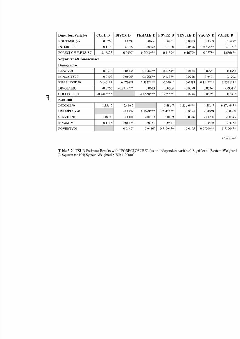
8/6/2019 Spatial Lag Regression
http://slidepdf.com/reader/full/spatial-lag-regression 191/268
1 7 7
Dependent Variable COLL_D DIVOR_D FEMALE_D POVER_D TENURE_D V
ROOT MSE (σ) 0.0760 0.0398 0.0606 0.0761 0.0813
INTERCEPT 0.1190 0.3627 -0.0492 0.7368 0.0506
FORECLOSURE(83–89) -0.1682* -0.0699+ 0.2563*** 0.1459* 0.1670*
Neighborhood Characteristics
Demographic
BLACK90 0.0373 0.0673* 0.1262** -0.1254* -0.0164
MINORITY90 -0.0403 -0.0596* -0.1266** 0.1338* 0.0268
FEMALEKID90 -0.1401** -0.0796** -0.5158*** 0.0904+ 0.0513 0
DIVORCE90 -0.0766 -0.8414*** 0.0623 0.0669 -0.0350
COLLEGEH90 -0.4443*** -0.0858*** -0.1225*** -0.0234
Economic
INCOME90 1.53e-7 -2.46e-7 1.48e-7 1.23e-6***
UNEMPLOY90 -0.0279 0.1699*** 0.2247*** -0.0764
SERVICE90 0.0807+ 0.0181 -0.0163 0.0169 0.0386
MNGMT90 0.1115 -0.0677* -0.0131 -0.0541
POVERTY90 -0.0340+ -0.0486+ -0.7100*** -0.0195 0
Table 5.7: ITSUR Estimate Results with “FORECLOSURE” (as an independent variable) SignifR-Square: 0.4104; System Weighted MSE: 1.0000)
22
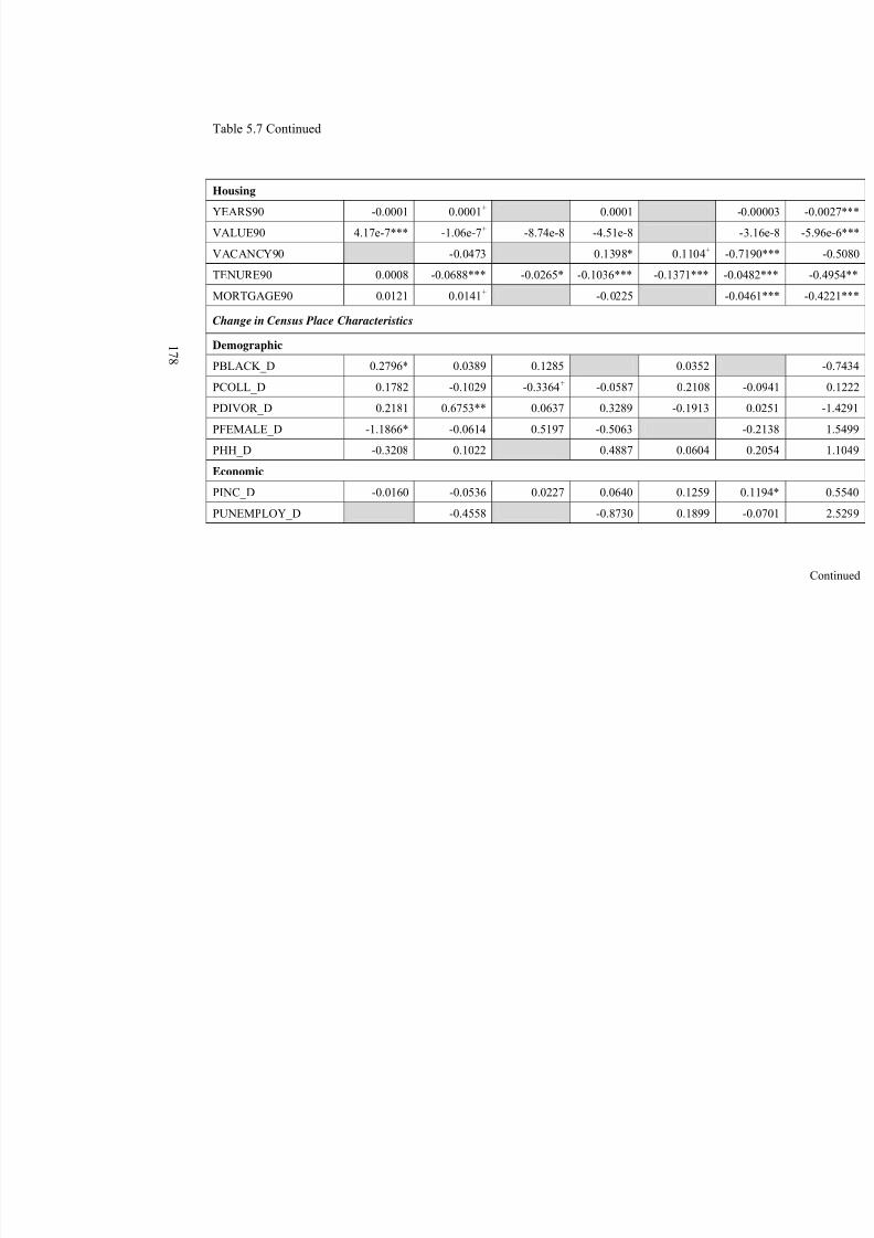
8/6/2019 Spatial Lag Regression
http://slidepdf.com/reader/full/spatial-lag-regression 192/268
1 7 8
Table 5.7 Continued
Housing
YEARS90 -0.0001 0.0001+ 0.0001
VALUE90 4.17e-7*** -1.06e-7+ -8.74e-8 -4.51e-8
VACANCY90 -0.0473 0.1398* 0.1104+ -0
TENURE90 0.0008 -0.0688*** -0.0265* -0.1036*** -0.1371*** -0
MORTGAGE90 0.0121 0.0141+ -0.0225 -0
Change in Census Place Characteristics
Demographic
PBLACK_D 0.2796* 0.0389 0.1285 0.0352
PCOLL_D 0.1782 -0.1029 -0.3364+ -0.0587 0.2108
PDIVOR_D 0.2181 0.6753** 0.0637 0.3289 -0.1913
PFEMALE_D -1.1866* -0.0614 0.5197 -0.5063
PHH_D -0.3208 0.1022 0.4887 0.0604
Economic
PINC_D -0.0160 -0.0536 0.0227 0.0640 0.1259
PUNEMPLOY_D -0.4558 -0.8730 0.1899
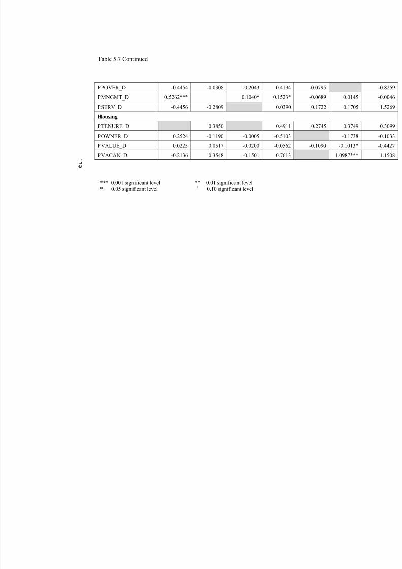
8/6/2019 Spatial Lag Regression
http://slidepdf.com/reader/full/spatial-lag-regression 193/268
1 7 9
Table 5.7 Continued
PPOVER_D -0.4454 -0.0308 -0.2043 0.4194 -0.0795
PMNGMT_D 0.5262*** 0.1040* 0.1523* -0.0689
PSERV_D -0.4456 -0.2809 0.0390 0.1722
Housing
PTENURE_D 0.3850 0.4911 0.2745
POWNER_D 0.2524 -0.1190 -0.0005 -0.5103
PVALUE_D 0.0225 0.0517 -0.0200 -0.0562 -0.1090
PVACAN_D -0.2136 0.3548 -0.1501 0.7613
*** 0.001 significant level ** 0.01 significant level* 0.05 significant level + 0.10 significant level

8/6/2019 Spatial Lag Regression
http://slidepdf.com/reader/full/spatial-lag-regression 194/268
180
Change Variables Associated with Foreclosures
As mentioned before there are seven change variables that are significantly related
to foreclosures: change in educational attainment (negative), change in percentage
divorced population (negative), change in female headship rate (positive), change in
percentage population below the poverty line (positive), change in homeownership rate
(positive), change in housing vacancy rate (negative), and change in median housing
value (positive). The foreclosure rate has different levels of significance in those
regression equations. In all other equations where the dependent variables are the other
change variables, foreclosure rate is not significant. The estimate results of those latter
equations are in Appendix D (Table D.1).
Change in Percentage Population with College or Higher Education (>25 years old)
The importance of residents’ educational attainment to the quality and stability of a
neighborhood has been stated in previous sections. In this analysis the research found that
foreclosure rates are negatively related to the change in percentage population with
college degrees or higher. This means that higher foreclosure rates in the previous time
period are associated with a lower increase (or a larger decrease) in the percentage
population with college degrees or higher. This is consistent with our expectations
because educational attainment is highly related to other household characteristics, and
thus can be related to foreclosures. Neighborhoods with higher foreclosures are usually
associated with poor neighborhood quality. Neighborhood decline associated with
foreclosures will be less attractive to populations with higher education attainment.
It is also possible that people with higher educational attainment move out of
8/6/2019 Spatial Lag Regression
http://slidepdf.com/reader/full/spatial-lag-regression 195/268
181
neighborhoods because of the expected impact of the rising foreclosure rates on housing
values, crime and other neighborhood indicators. On the other hand, the lower increase or
larger decrease in educational attainment associated with higher foreclosure rates might
be because the neighborhoods with higher foreclosure rates have characteristics that
attract people with lower educational attainment, thus the in-movement of those people
will lower the general educational attainments of the residents in those neighborhoods.
Change in Percentage Divorced Population (>16 years old)
It is interesting to see that foreclosures are associated with the change in percentage
divorced population in a negative way. This means that higher foreclosure rates in the
previous time period are related to lower increase (or higher decrease) in the percentage
divorced population in a neighborhood. There are several potential explanations for this
phenomenon.
The first one is that more divorced people had their homes foreclosed and moved
out of the neighborhoods. Foreclosures can be caused by the financial shock of a divorce
and divorced householders may be at more risk of other financial problems. On the other
hand, it is also possible that the foreclosed homes are attractive to singles or married
couples, especially those first-time homebuyers who can only afford the discounted price
of those foreclosed houses. Another possibility would be gentrification pioneers (those
who are not divorced) purchasing the foreclosed properties from which divorced
households move out.
8/6/2019 Spatial Lag Regression
http://slidepdf.com/reader/full/spatial-lag-regression 196/268
182
Change in Female Headship Rate
The female headship rate is widely used to measure neighborhood quality (Galster
and Krall, 2003) and how welfare policy and benefits affect family structure (especially
the formation of female-led households) (Moffitt, 2000). Female-led households are
vulnerable to various financial and housing hardships, and are often the victims of
predatory lending (CRL, 2004). According to the Center for Responsible Lending (CRL),
female-led households also account for a larger share of subprime loans than of prime
loans. Given all these entire issues associated with female-led households, it is not
surprising to see that foreclosures have a positive relationship with the change in female
headship rate. This means that higher foreclosure rates in the previous time period are
associated with faster increases (or slower decreases) in the percentage of female-led
households.
Higher foreclosures usually happen in neighborhoods with higher percentage
female-led households. And many of those households are minority, especially black
households. Because those female-led households are in a more vulnerable financial
situation on average they are more likely to become victims of foreclosure. Even if many
of those householders are renters, the clustering of this type of households is often
associated with poor neighborhood quality. In such a neighborhood if a homeowner gets
in trouble there is less reason to try to work out the problem and it is more likely that the
homeowners will give up the property to foreclosure and move away. When the higher
foreclosure rates and the concentration of female-led households are highly associated
with each other, creates an even more vulnerable environment for female-led households.
Policy makers might want to pay more attention to neighborhoods with concentrations of
8/6/2019 Spatial Lag Regression
http://slidepdf.com/reader/full/spatial-lag-regression 197/268
183
female-led households. It might also be a good idea to initiate programs to help those
households in dealing with the stress and impacts of foreclosures.
Change in Percentage Population below the Poverty Line
The research found that foreclosures have a positive relationship with the change in
percentage population below the poverty line. This means that higher foreclosures
between 1983 and 1989 are associated with a larger increase (or a slower decrease) in the
percentage population below the poverty line during the subsequent decade. Thus higher
foreclosures are related to the neighborhoods that are more likely to have a concentration
of population below the poverty line.
Higher foreclosures can make a neighborhood less attractive to people with higher
income because of the decreased quality of houses and neighborhoods. On the one hand
higher foreclosures will increase housing vacancy rates when homeowners are forced to
move out of the neighborhood because of foreclosures or simply because of the
deteriorated neighborhood and housing quality. The loss of homeowners can increase the
percentage population below the poverty line in the neighborhoods. On the other hand,
even if the foreclosed houses are occupied again, the new owners or renters might be
those with lower income, even those below the poverty line, since the home is likely to be
sold at a discount. This can contribute to the increase in percentage population below the
poverty line. Homeowners who have not been foreclosed are also likely to leave
neighborhoods with high foreclosure rates and those homes may be subdivided for rental
to lower income groups.
8/6/2019 Spatial Lag Regression
http://slidepdf.com/reader/full/spatial-lag-regression 198/268
184
Change in Homeownership Rate
The importance of homeownership has been stated by many scholars in their
research, and the interaction between the homeownership rate and foreclosures is very
important and can have significant policy implications. This research has very important
findings in terms of the relationships between the two. Both the homeownership rate and
the change in the rate have been found to affect foreclosure rates in the preceding
analysis of neighborhood effects on foreclosures. In this section the research found that
foreclosures in a previous time period are associated with the later change in the
homeownership rate in a positive manner. This means that an increase in foreclosure rates
is associated with an increase or slower decrease in the homeownership rate. This seems
to be the opposite of what we expected. This might mean that higher foreclosures in some
neighborhoods will cause housing values to drop, thus attracting lower income people
moving into those neighborhoods to become homeowners, even to occupy the previously
vacant properties or rental properties. This is a very important possibility given how often
we try to get more owners in a neighborhood by getting poorer people (more likely to
have a foreclosure) into owner-occupied houses in those neighborhoods.
When foreclosure rates rise in a neighborhood there will be more vacant housing
units. Many of those houses (even those who are not foreclosed in the research time
period) are purchased by people. Therefore, the neighborhood may gain some owners
because of the foreclosure. Another possible reason is that gentrification can happen in
those neighborhoods with higher foreclosures (and lower values), and thus the process of
gentrification can improve the homeownership rate in those neighborhoods.
8/6/2019 Spatial Lag Regression
http://slidepdf.com/reader/full/spatial-lag-regression 199/268
185
On the other hand, if a neighborhood is experiencing decreasing homeownership
rate, increasing foreclosure rates will slow down the decreasing process.
Foreclosures being positively associated with increases in homeownership rates in
Cuyahoga County, is difficult to explain. It may be accurate with the some possible
explanations listed above or there may be omitted variables that were not controlled.
Further investigation can be helpful if there are data available in other geographic areas,
or if there are other important variables to include.
Change in Housing Vacancy Rate
The housing vacancy rate has been found to positively contribute to foreclosures in
previous neighborhood effects research. In this analysis of the impact of foreclosures on
neighborhood change the results indicate that foreclosures have a negative relationship
with housing vacancy rates. This means that higher foreclosures in a previous time period
are associated with slower increases (or faster decreases) of housing vacancy rates in the
subsequent decade. This is also an unexpected result, similar to the relationship between
foreclsoures and the change in the homeownership rate. It might be because higher
foreclosures will bring investors to those foreclosed properties (including the ones
foreclosed beyond the research time period) and those properties are converted to rental
properties (with higher value than they had as owner occupied properties – especially if
subdivided). Another explanation could be the effect of redevelopment and/or
gentrifications. These processes will reduce vacant housing units in those neighborhoods.
Concentrations of foreclosures (higher foreclosure rates) might attract various kinds of
investors to inexpensive properties. If these investors are gentrifiers, in particular, the
8/6/2019 Spatial Lag Regression
http://slidepdf.com/reader/full/spatial-lag-regression 200/268
186
time gap between the two sets of data used in this analysis could allow for improvements
in the units, decreases in vacancy rates and increases in property values.
Change in Median Housing Values
As mentioned in the previous section of neighborhood effects research, the
relationship between the change in median housing value and foreclosures has different
results in the two counties. In Franklin County, change in median housing value is
negatively related to subsequent foreclosure rates, but in Cuyahoga County change in
median housing value is positively related to subsequent foreclosure rates. In this analysis
of the impact of foreclosures on later housing values we found that foreclosures have a
positive relationship with change in median housing value in Cuyahoga County. This
seems odd and deserves more research. Although we argue that urban redevelopment
policies and gentrification might cause this effect, it is also possible that omitted
variables, time differences between the data sets and data collection errors might also
contribute to this unexpected phenomenon.
The results indicate that higher foreclosures are associated with a larger increase (or
a slower decrease) in median housing values. In this situation, when two neighborhoods
both have an increased median housing value, the one with a higher foreclosure rate will
be associated with a larger increase in the value (might be associated with subsequent
revitalization or gentrification processes). When two neighborhoods both have a
decreased median housing value a higher foreclosure rate is associated with a slower
decrease in median housing value (might be associated with increased housing values due
to renovated foreclosed properties). If one neighborhood has an increased median

8/6/2019 Spatial Lag Regression
http://slidepdf.com/reader/full/spatial-lag-regression 201/268
187
housing value and the other one has a decreased median housing value, the neighborhood
with a higher foreclosure rate is the one with an increased median housing value.
8/6/2019 Spatial Lag Regression
http://slidepdf.com/reader/full/spatial-lag-regression 202/268
188
Conclusion: The Interaction between Residential Mortgage Foreclosure,
Neighborhood Characteristics, and Neighborhood Change
The interaction between residential mortgage foreclosure and neighborhood
characteristics and change is very complicated and there are many factors related to the
issue. However, this research finds some very interesting phenomena among the
relationship. The two elements interact with each other in terms of specified
neighborhood indicators and their changes. The research results do not support all of the
initial hypotheses, and so contradict some previous research on the topic.
First of all, neighborhood characteristics and change in the immediately proceeding
time period affects foreclosure rates. Many factors are involved, although some of the
effects are different for the two study counties. Common factors affecting foreclosures
for the two counties are percentage population with college degrees or higher, median
household income, and average housing cost burden. In Cuyahoga County percentage
black population and the change in this percentage has a positive relationship with
foreclosures. However, foreclosure does not affect the change in percentage black
population in Cuyahoga County. This finding is very different from what Baxter and
Lauria (2000) found in the relationship between foreclosures and racial turnover in New
Orleans. It is difficult to determine which finding is more appropriate because there are
many differences in social-economic characteristics in different places. If some of the
characteristics are not controlled there will be inconsistent results from the analyses. The
results may also indicate the importance of local context to the impact of foreclosure.
There are also some unique attributes in the neighborhood effects of each county.
When looking at demographic characteristics and change we found that percentage black
8/6/2019 Spatial Lag Regression
http://slidepdf.com/reader/full/spatial-lag-regression 203/268
189
population and the change in percentage black population has an impact on foreclosures
in Cuyahoga County, which is not the case in Franklin County. From the point of view of
economic characteristics and change, percentage labor force employed in service
occupation affects foreclosures in Franklin County, while percentage population below
the poverty line and the change in the percentage affect foreclosures in Cuyahoga
County. Besides the common housing factor change in homeownership rate, change in
housing vacancy rate and change in median housing value are all negatively affect
foreclosures in Franklin County, while homeownership rate, percentage housing units
with a mortgage, and change in owner-occupied housing units affect foreclosures in
Cuyahoga County. The reasons for these differences between counties need further
exploration.
When we examine whether and how foreclosures affect neighborhood change in
Cuyahoga County using the 1983-1989 foreclosure data we found that there are seven
change variables from 1990 to 2000 that are significantly related to those earlier
foreclosures: change in educational attainment (negatively), change in percentage
divorced population (negatively), change in female headship rate (positively), change in
percentage population below the poverty line (positively), change in homeownership rate
(positively), change in housing vacancy rate (negatively), and change in median housing
value (positively). Among those relationships the ones between change in
homeownership, change in housing vacancy rate, and change in median housing value are
different from what we expected. We argued that perhaps neighborhood revitalization,
renovation of the foreclosed properties, and/or gentrification might contribute to those
relationships. Also data collection errors, omitted variables, the correlation between the
8/6/2019 Spatial Lag Regression
http://slidepdf.com/reader/full/spatial-lag-regression 204/268
190
change variables at the neighborhood level, the relatively long time span between the
beginning of one data set and the end of the other and spatial effects might also make the
estimated results somewhat difficult to interpret. Thus using simultaneous spatial models
might resolve some of those issues. But it is difficult to find an instrument variable to
help identify the simultaneous equations. Also incorporating spatial effects into
simultaneous equation models might be very challenging. These would be fruitful areas
for future research.
If we draw a diagram to see how neighborhood characteristics and change interact
with foreclosures (see Figure 5.1) we find that change in percentage population below the
poverty line is the only factors with mutually interactive relationship with foreclosures in
Cuyahoga County. Other neighborhood characteristics and change variables only interact
with foreclosures in a one way direction. However, we notice that the change in median
housing value negatively affects foreclosures in Franklin County, but in Cuyahoga
County it is not related to foreclosures. This is very interesting and deserves further
investigation. In Cuyahoga County the change in percentage population below the
poverty line yields opposite signs in the neighborhood effects analysis versus the impact
analysis of foreclosures. It is negatively related to foreclosures when we examine them as
precursors to the foreclosure rate. When foreclosures are used to explain neighborhood
change variables (foreclosure rates in an earlier time period affect neighborhood change
in a later time period) the effect of foreclosure rates is positive. Please refer to the
previous detailed narratives for potential reasons explaining this phenomenon.
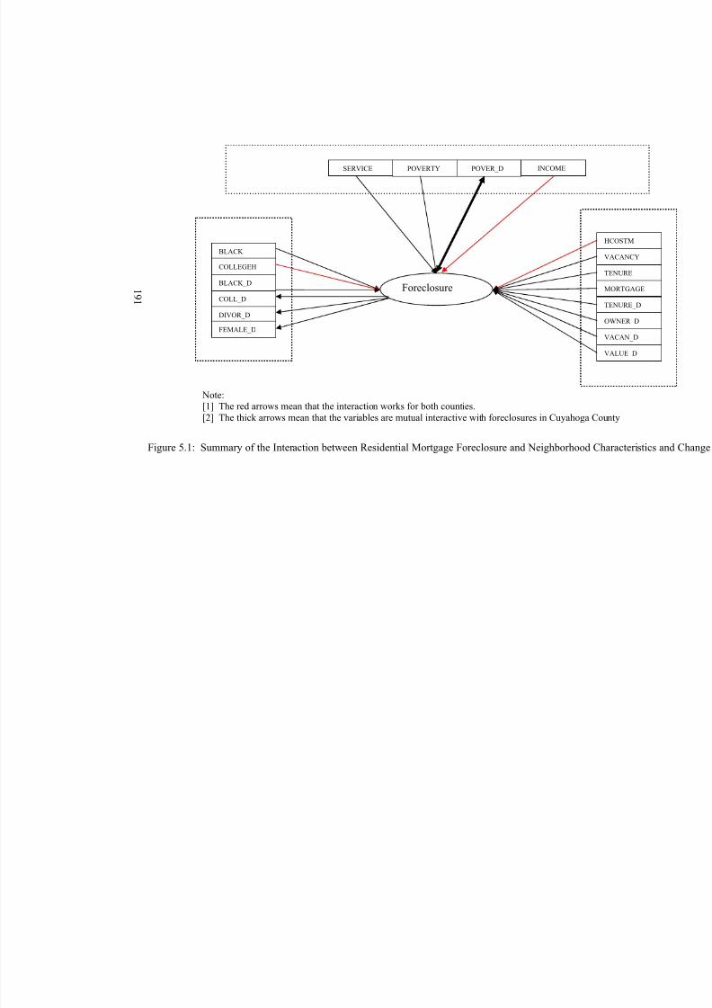
8/6/2019 Spatial Lag Regression
http://slidepdf.com/reader/full/spatial-lag-regression 205/268
1 9 1
Note:
[1] The red arrows mean that the interaction works for both counties.[2] The thick arrows mean that the variables are mutual interactive with foreclosures in Cuyahoga C
BLACK
COLLEGEH
BLACK_D
COLL_D
DIVOR_D
POVER_DPOVERTYSERVICE
Foreclosure
FEMALE_D
INCOME
Figure 5.1: Summary of the Interaction between Residential Mortgage Foreclosure and Neighborhood C
8/6/2019 Spatial Lag Regression
http://slidepdf.com/reader/full/spatial-lag-regression 206/268
192
CHAPTER 6
CONCLUSIONS, POLICY IMPLICATIONS AND
FUTURE RESEARCH DIRECTIONS
As mentioned in previous chapters the relationship between residential mortgage
foreclosure and neighborhood characteristics and change is very complicated and is
related to many aspects of the issue. However, this research has helped us understand
more about the relationship. The research methodology and results can provide useful
insights to both theory and policy in foreclosure research. The research can also serve as
a pilot study for larger future research projects. At the beginning the research proposed
three research questions and several sets of hypotheses. The findings answered most of
the questions, although not all hypotheses were supported.
The first research question is whether and how neighborhood characteristics and
change affect foreclosures. Our results indicate that neighborhood characteristics and
change affect foreclosures in a profound manner. First we examined the spatial patterns
of foreclosure rates and found that foreclosures rates are spatially autocorrelated across
neighboring block groups. This indicates that foreclosures may be spatially contagious.
We would also expect that foreclosures in one time period will be spatially autocorrelated
with neighborhood indicators in neighboring block groups in the following time period.
We also found strong heteroskedasticity in the data sets of both counties. The
8/6/2019 Spatial Lag Regression
http://slidepdf.com/reader/full/spatial-lag-regression 207/268
193
neighborhood effects in the two study counties share some common attributes, although
there are disparities between the results for the two counties as well.
The independent variables were divided into three categories of neighborhood
characteristics and change, demographic, economic and housing. These three categories
all affect foreclosures in a similar way in both counties through the variables educational
attainment (demographic), median household income (economic) and average housing
cost burden (housing). There are some differences in the neighborhood effects on
foreclosures between the two counties. The most important difference that is related to
our hypothesis is that racial composition and turnover affect foreclosures only in
Cuyahoga County. Change in median housing value has a positive effect on foreclosures
in Franklin County but there is on effect in Cuyahoga County. The detailed explanation
can be found in Chapter 5.
The second question is whether and how foreclosures affect neighborhood change.
Our results found that foreclosures in a previous time period do affect some
neighborhood change indicators for the subsequent decade. Higher foreclosure rates are
related to increases in the less educated population, female-led households and the poor
population in neighborhoods. Foreclosure rates are negatively related to the percentage
divorced population.
The relationships between foreclosure rates and the change in homeownership rate,
the change in housing vacancy rate, and the change in median housing value in Cuyahoga
County have results that are not consistent with our expectations. We expected that
foreclosures would hinder the increase in homeownership rates, but the research results
indicate that foreclosure rates are positively related to the change in homeownership
8/6/2019 Spatial Lag Regression
http://slidepdf.com/reader/full/spatial-lag-regression 208/268
194
rates. We also expected that foreclosures would aggravate housing vacancy issues in a
neighborhood, but the results indicate that foreclosure rates are negatively related to the
change in housing vacancy rate. We expected that foreclosures would decrease housing
value appreciation or speed up depreciation, but the results indicate that foreclosure rates
are positively related to the change in median housing values. While data issues may be a
problem, revitalization and gentrification of declining neighborhoods and investor
behavior (subdivision, renovation or flipping of the foreclosed properties) might help
explain the research results as well. In the future when data from more geographic areas
are available more research can be done to test whether the effects happen in other places
and what contextual variables affect the relationships. At the same time a spatial
simultaneous equation model might be constructed and estimated with the same dataset.
However, it will be very challenging to identify the estimation techniques related to the
spatial simultaneous equation models. Resolving identification problems associated with
simultaneous equations becomes more difficult when there are a large number of related
variables and non-recursive causal relationships in the model.
The third question asked at the beginning of the research is related to developing a
model that can separate the two effects. The use of panel data made it possible to separate
the effect of neighborhood characteristics on foreclosures from the effect of foreclosures
on neighborhoods, and the use of spatial analysis, spatial regression, heteroskedasticity
correction and Seemingly Unrelated Regression (SUR) contributed significantly to the
research methodology on this topic. However, even if we use panel data (foreclosures in
1983-1989 affect neighborhood change from 1990 to 2000; and then neighborhood
characteristics in 2000 and change from 1990 to 2000 affect foreclosures in 2001-2004)
8/6/2019 Spatial Lag Regression
http://slidepdf.com/reader/full/spatial-lag-regression 209/268
195
other factors, such as policy change, omitted variables, and collinearity between the
variables, will affect the estimation results. As indicated above, a goal for future research
should be to combine the separate effects in a simultaneous equation model.
When looking at the sets of hypotheses in detail we found that the findings
supported some of the initial expectations but not others.
The research finds that foreclosures concentrate in certain neighborhoods over time
and strong spatial autocorrelation in foreclosure rates exists. These findings support our
expectations.
In terms of the interaction between foreclosures and change in housing value the
research did not support the idea that housing value depreciation contributes to
foreclosures, although change in housing value does negatively affect foreclosures in
Franklin County. This means that the drops in housing value in the earlier time period are
associated with increases in the foreclosure rates as we would expect. The SUR found
that foreclosure rates in the earlier time period significantly and positively contribute to
the change in median housing value in a neighborhood in Cuyahoga County. This is very
different from what we expected. Therefore, the interaction between housing value and
foreclosures at a neighborhood level is more complex than that the literature indicates
and needs further investigation.
When exploring the effect of racial composition on foreclosure rates the research
found that percentage black population and its change affect foreclosures only in
Cuyahoga County. In Franklin County, racial composition does not directly contribute to
foreclosure rates. On the other hand, the SUR found that foreclosures do not affect the
change in racial composition of a neighborhood in Cuyahoga County. Therefore, the
8/6/2019 Spatial Lag Regression
http://slidepdf.com/reader/full/spatial-lag-regression 210/268
196
research does not support our initial hypothesis that racial factors would contribute to
foreclosures in both counties (it is not true in Franklin County), nor do the findings
support our expectations that foreclosures affect racial turnover of a neighborhood. So the
findings of the relationship between racial composition and foreclosures are not
consistent with research by Baxter and Lauria (2000) in New Orleans. This might
because some place-related characteristics are not controlled in either or both of the
studies, thus the results are different. For example, New Orleans might also be more
racially segregated than Cuyahoga County, and thus foreclosure will acerbate the
segregation. It is important that future research consider multiple geographic areas and
their racial contexts in order to shed more light on this issue.
For both counties median household income is positively related to foreclosures.
This does not support our initial hypothesis that median household income would be
negatively related to foreclosures. Perhaps the increase in housing cost burden has offset
the benefits of gaining income, thus higher income will be related to higher foreclosure
rates. On the other hand, foreclosure rates do not affect the change in income in our
Cuyahoga County analysis.
Housing vacancy rates in an earlier time period are significantly related to
foreclosure rates in Franklin County in the later time period in a positive way, as we
expected. But foreclosure rates in the earlier period are negatively associated with the
change in the housing vacancy rate in Cuyahoga County during the subsequent decade.
The two counties are different in terms of demographic, economic and housing
characteristics and change. Therefore the interaction between residential mortgage
foreclosure and neighborhood characteristics and change is different, although there are

8/6/2019 Spatial Lag Regression
http://slidepdf.com/reader/full/spatial-lag-regression 211/268
197
some common findings in both counties. In particular, the economic and racial context of
the two counties underlies some of the differences that we have discovered.
The research has answered most of the research questions, and some results indicate
important directions for future research.

8/6/2019 Spatial Lag Regression
http://slidepdf.com/reader/full/spatial-lag-regression 212/268
198
Policy Implications
Concern about foreclosure and its impact on homeowners and neighborhoods has
promoted research and policy innovations in recent years. One of the purposes of this
project is to provide information to policy makers to help in understanding the
relationship between residential mortgage foreclosure and neighborhood characteristics
and change. Therefore, the research findings have significance in helping address
foreclosure issues.
For both counties foreclosures have concentrated in certain neighborhoods. These
are usually inner city areas, although there are some scattered cases stretching to the
suburbs, especially in later years. Therefore policy makers should pay particular attention
to those neighborhoods with clustered foreclosure cases. However, since there are many
factors affecting foreclosures and the factors vary somewhat between counties, each of
those neighborhoods should have tailored programs for foreclosure prevention. For both
counties, educational attainment is one of the demographic factors related to foreclosure
rates. Policy makers can try to promote educational attainment and it can be incorporated
into community development policies. If the effect of educational attainment on
foreclosures lies in the fact that more educated people do not easily become the victims
of predatory lending, then financial education to the residents might help prevent
foreclosures, and all neighborhood residents would benefit, especially in those
neighborhoods with low educational attainment.
The research found that decreasing housing cost burden in a neighborhood is related
to decreasing foreclosure rates. Policy makers might initiate funds to help alleviate
housing cost burdens, especially for highly cost burdened homeowners in high cost
8/6/2019 Spatial Lag Regression
http://slidepdf.com/reader/full/spatial-lag-regression 213/268
199
burden neighborhoods. Decreasing housing vacancy rates in a neighborhood is also
related to decreasing foreclosure rates and also helps diminish the clustering of foreclosed
homes. Policy can encourage redevelopment for areas with high vacancy rates, or
encourage real estate investors to purchase vacant properties. This latter policy would
have to guard against flippers and predatory lenders who could simply make the problem
worse. The goals of all those policies cannot be achieved in a short time and there might
be many obstacles in implementing the policies. However, the research provides a
foundation for policy makers to refer to when making policy changes and it argues for
policies aimed at neighborhoods, not just policies aimed at individual homeowners. This
is particularly important because of the clear spatial clustering and probable contagion
effect in foreclosures.
As the impact of foreclosure on neighborhood change variables indicates, change in
female headship rate and change in homeownership rate are positively related to
foreclosures in Cuyahoga County. These relationships could lead to increased involuntary
income segregation or concentration of the low income population in neighborhoods with
high foreclosures (and thus weakens housing appreciation and other market indicators).
Policy makers can focus on the neighborhoods with an increasing percentage of female
headship rate and/or an increase in percentage population below the poverty line with
pre-foreclosure prevention and post foreclosure remedial programs (see Figure 6.1 and
Figure 6.2 for the change in female headship rate and the change in percentage
population below the poverty line). However, this does not mean that we should not put
any efforts into other neighborhoods.
8/6/2019 Spatial Lag Regression
http://slidepdf.com/reader/full/spatial-lag-regression 214/268
200
Generally speaking foreclosure prevention should not be the same in all places. Each
neighborhood has unique characteristics and patterns of change and each county has a
unique economic and demographic context. Therefore, when we seriously work to
prevent foreclosures we need to have an individualized program for each neighborhood
that is vulnerable to foreclosures. The research has provided some specified findings in
terms of what neighborhood characteristics and change variables will affect foreclosure
rates, and what neighborhood change variables are affected by foreclosures. Hopefully
the significance of the research for policy making can be recognized in this way.
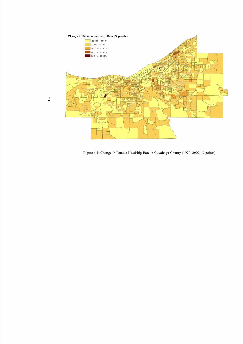
8/6/2019 Spatial Lag Regression
http://slidepdf.com/reader/full/spatial-lag-regression 215/268
2 0 1
Change in Femaile Headship Rate (% points)
-30.59% - 0.0000
0.01% - 10.00%
10.01% - 20.00%
20.01% - 30.00%
30.01% - 50.00%
Figure 6.1: Change in Female Headship Rate in Cuyahoga County (1990–2000, %
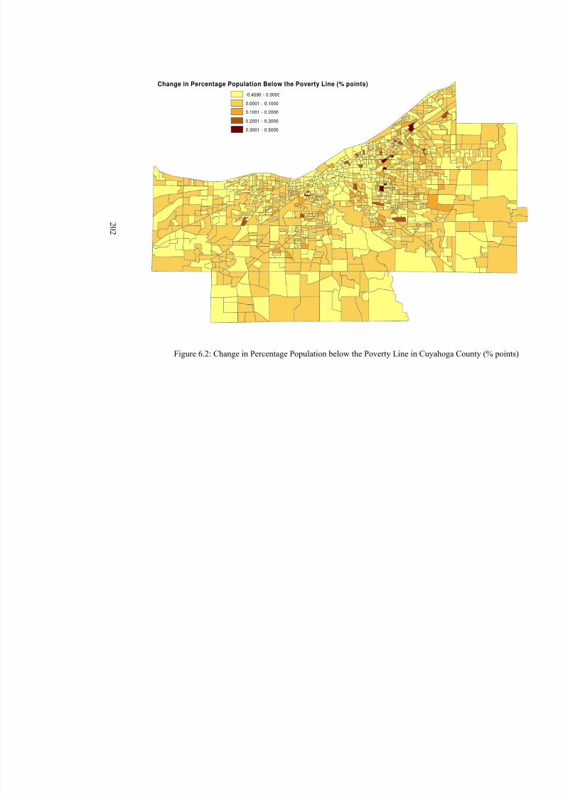
8/6/2019 Spatial Lag Regression
http://slidepdf.com/reader/full/spatial-lag-regression 216/268
2 0 2
Change in Percentage Population Below the Poverty Line (% points)
-0.4590 - 0.0000
0.0001 - 0.1000
0.1001 - 0.2000
0.2001 - 0.3000
0.3001 - 0.5000
Figure 6.2: Change in Percentage Population below the Poverty Line in Cuyahoga Coun

8/6/2019 Spatial Lag Regression
http://slidepdf.com/reader/full/spatial-lag-regression 217/268
203
Future Research Directions
Since this research explores the mutual interaction between residential mortgage
foreclosure and neighborhood characteristics and change, the research results can be used
as the foundation for a Structural Equation Model that incorporates the separate effects
into one model. Thus the methodology can be changed to see how consistent the results
will be. Ideally spatial effects would be considered although this makes the
methodological task even more challenging. This should be the first step in future
research on the topic. However, when exploring the impact of foreclosures on
neighborhood change, a spatial simultaneous model can be separately constructed, if
feasible, thus resolving some issues in the current SUR model (such as the omitted
variables, non-recursive relationships, and others).
Another path to use in studying the impact of foreclosures on neighborhood change
could focus on using spline regression models to capture the “threshold effects”. These
possible effects suggest that the relationships are not continuous, but rather that there is
little effect from a particular variable until a “threshold” is reached and then the effect is
relatively large. For example, it would be valuable to find out at what point foreclosures
will contribute to neighborhood change positively, or negatively, or at what point
neighborhood characteristics become important to foreclosures.
As far as other methodological issues go, future research should try to find a viable
approach for running the spatial regression models controlling for both heteroskedasticity
and spatial autocorrelation at the same time, and then compare the results with those in
this research. The purpose of the comparison is to see if separately controlling for
heteroskedasticity and spatial autocorrelation yields similar results as running the model
8/6/2019 Spatial Lag Regression
http://slidepdf.com/reader/full/spatial-lag-regression 218/268
204
by controlling the two problems simultaneously. Ideally we should also pay attention to
other issues associated with the spatial regression models, such as omitted variables, data
improvements, and multicollinearity.
Many of the research findings are very interesting, but need further investigation.
One of the future research directions is to find out why some neighborhood
characteristics and changes contribute to foreclosures and others do not. And on the other
hand, why certain neighborhood change variables are related to foreclosures but others
are not. When we want to know the relationship of an individual neighborhood factor and
foreclosures we can only focus on one factor, such as the relationship between racial
turnover and foreclosure, the relationship between the female headship rate and
foreclosure, or the relationship between the homeownership rate and foreclosure.
The biggest problem in this research lies in data and time limitations. Sheriff’s real
estate sales data and court records can be easily accessed through many approaches, but
they usually do not have the data format that an academic researcher needs. To rebuild
the data consumes time. Therefore, given time and budget, future research can use those
data and merge them with multiple years’ Home Mortgage Disclosure Act (HMDA) data
and county property transaction data to find out how loan and borrowers’ characteristics,
as well as housing attributes at the loan’s origination can affect foreclosure. This will be
much more accurate than simulations of default probability using HMDA data at the loan
origination such as those performed by Ambrose and Sanders (2002). The research can
expand to using data from other states in the U.S. to find out the relations between real
mortgage default and loan and borrowers’ characteristics at the loan origination. The
result will provide more reliable underwriting standards for lenders. In addition,
8/6/2019 Spatial Lag Regression
http://slidepdf.com/reader/full/spatial-lag-regression 219/268
205
research should examine the relationship between foreclosure filings and sheriff sale
properties. What happens to the properties that are foreclosed but do not go to sheriff’s
sales and do they have different relationships with neighborhood variables?
Another aspect of the future research is to track the addresses of the borrowers
whose properties were foreclosed and conduct a survey to explore the reasons why they
defaulted, the impact of the default on them and where they moved. This will be very
helpful to learn how borrower characteristics affect default decisions and foreclosure
risks.
The tracking of addresses includes both tracking where the borrowers go after
foreclosure and civic real estate sales, and also who buys the foreclosed properties and
what they do with them. The negative impact of foreclosure on a homeowner is very
significant. After losing their homes borrowers will have different tenure and moving
selections. Whether they choose to rent or buy again (and over what time period) and
where they move will affect neighborhood changes greatly, in both their previous
neighborhoods and their future neighborhoods. There are a variety of other questions
about those who have defaulted and lost their homes to foreclosure. There is no
assistance program helping them recover from the financial and emotional stress from
foreclosure. The other interesting set of questions refers to those who bought the
foreclosed properties. What are the buyers’ characteristics and what impact do they have
on the neighborhoods in which the properties are located? Other questions, such as how
foreclosure affects children’s school outcomes and individual development can also be
explored. All those questions are very challenging and interesting but no literature has
addressed them.
8/6/2019 Spatial Lag Regression
http://slidepdf.com/reader/full/spatial-lag-regression 220/268
206
Another direction for the future research is to find out why lenders choose
foreclosure, not other alternatives to resolve a troubled mortgage. Default decisions are
usually made by borrowers. But it is up to lenders to choose ways to resolve a troubled
loan. Is the decision based on cost effectiveness, or other reasons? Is there any racial or
geographic bias when lenders choose whose mortgage will be foreclosed, whose
mortgage will be modified, when there will be foreclosure sales, or when other
alternatives will be preferred?
Since the research in foreclosure and its impact on borrowers, lenders and the
neighborhoods is not mature, there are many directions for research related to
foreclosures. The research reported here provides a first step and thus contributes to the
scanty literature in this field.

8/6/2019 Spatial Lag Regression
http://slidepdf.com/reader/full/spatial-lag-regression 221/268
207
APPENDIX A
FORECLOSURE PROCEDURES
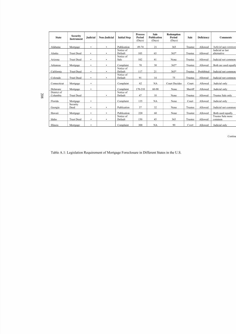
8/6/2019 Spatial Lag Regression
http://slidepdf.com/reader/full/spatial-lag-regression 222/268
2 0 8
StateSecurity
InstrumentJudicial Non-Judicial Initial Step
ProcessPeriod (Days)
SalePublication
(Days)
RedemptionPeriod(Days)
Sale
Alabama Mortgage • • Publication 49-74 21 365 Trustee
Alaska Trust Deed • • Notice of Default 105 65 365* Trustee
Arizona Trust Deed • • Notice of Sale 102 41 None Trustee
Arkansas Mortgage • • Complaint 70 30 365* Trustee
California Trust Deed • • Notice of Default 117 21 365* Trustee
Colorado Trust Deed • • Notice of Default 91 14 75 Trustee
Connecticut Mortgage • Complaint 62 NA Court Decides Court
Delaware Mortgage • Complaint 170-210 60-90 None Sheriff District of Columbia Trust Deed •
Notice of Default 47 18 None Trustee
Florida Mortgage • Complaint 135 NA None Court
GeorgiaSecurityDeed • • Publication 37 32 None Trustee
Hawaii Mortgage • • Publication 220 60 None Trustee
Idaho Trust Deed • • Notice of Default 150 45 365 Trustee
Illinois Mortgage • Complaint 300 NA 90 Court
Table A.1: Legislation Requirement of Mortgage Foreclosure in Different States in the U.S.
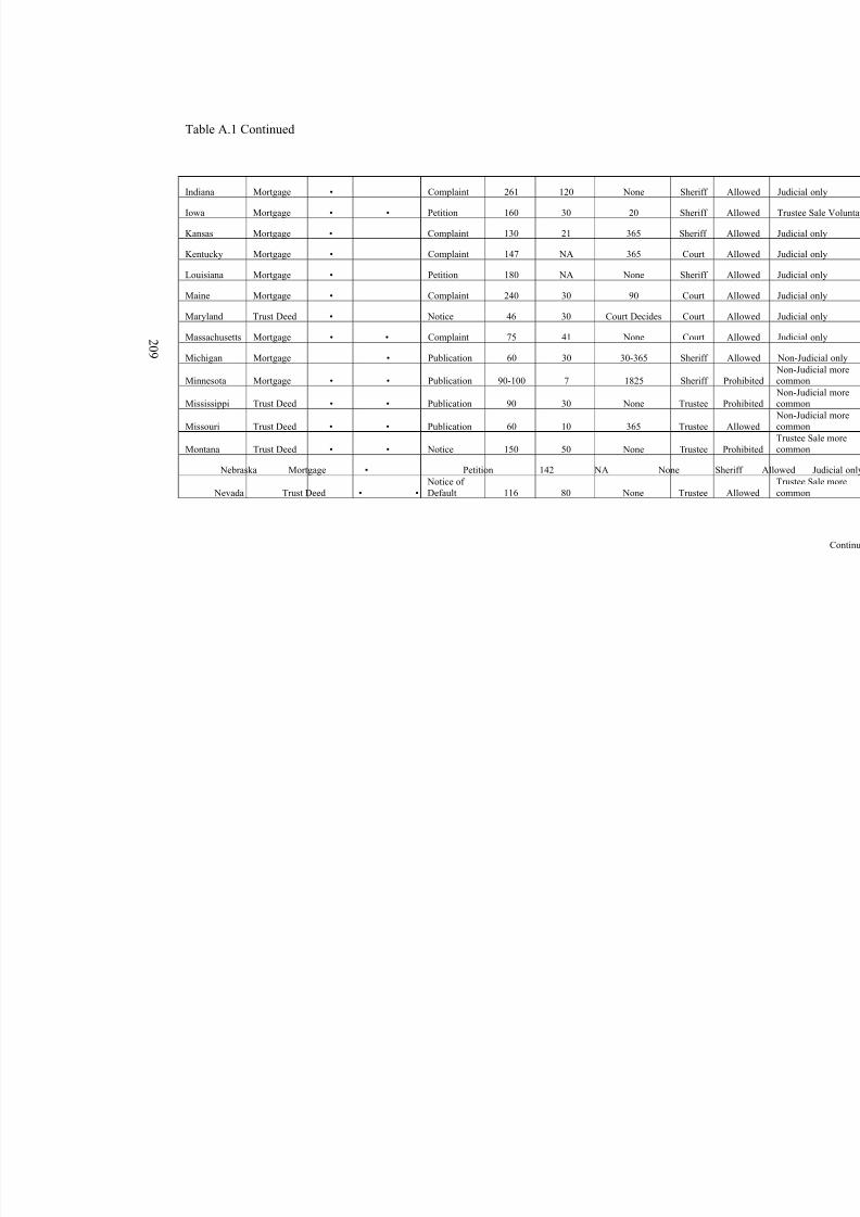
8/6/2019 Spatial Lag Regression
http://slidepdf.com/reader/full/spatial-lag-regression 223/268
2 0 9
Table A.1 Continued
Indiana Mortgage • Complaint 261 120 None Sheriff
Iowa Mortgage • • Petition 160 30 20 Sheriff
Kansas Mortgage • Complaint 130 21 365 Sheriff
Kentucky Mortgage • Complaint 147 NA 365 Court
Louisiana Mortgage • Petition 180 NA None Sheriff
Maine Mortgage • Complaint 240 30 90 Court
Maryland Trust Deed • Notice 46 30 Court Decides Court
Massachusetts Mortgage • • Complaint 75 41 None Court
Michigan Mortgage • Publication 60 30 30-365 Sheriff
Minnesota Mortgage • • Publication 90-100 7 1825 Sheriff
Mississippi Trust Deed • • Publication 90 30 None Trustee
Missouri Trust Deed • • Publication 60 10 365 Trustee
Montana Trust Deed • • Notice 150 50 None Trustee
Nebraska Mortgage • Petition 142 NA None S
Nevada Trust Deed • •
Notice of
Default 116 80 None Trustee
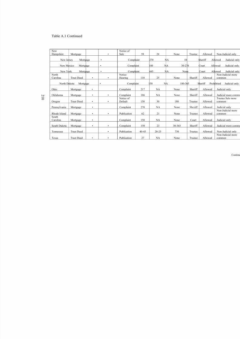
8/6/2019 Spatial Lag Regression
http://slidepdf.com/reader/full/spatial-lag-regression 224/268
2 1 0
Table A.1 Continued
NewHampshire Mortgage •
Notice of Sale 59 24 None Trustee
New Jersey Mortgage • Complaint 270 NA 10 Sh
New Mexico Mortgage • Complaint 180 NA 30-270 Co
New York Mortgage • Complaint 445 NA None C
NorthCarolina Trust Deed • •
NoticeHearing 110 25 None Sheriff
North Dakota Mortgage • Complaint 150 NA 180-365 She
Ohio Mortgage • Complaint 217 NA None Sheriff
Oklahoma Mortgage • • Complaint 186 NA None Sheriff
Oregon Trust Deed • • Notice of Default 150 30 180 Trustee
Pennsylvania Mortgage • Complaint 270 NA None Sheriff
Rhode Island Mortgage • • Publication 62 21 None Trustee
SouthCarolina Mortgage • Complaint 150 NA None Court
South Dakota Mortgage • • Complaint 150 23 30-365 Sheriff
Tennessee Trust Deed • Publication 40-45 20-25 730 Trustee
Texas Trust Deed • • Publication 27 NA None Trustee
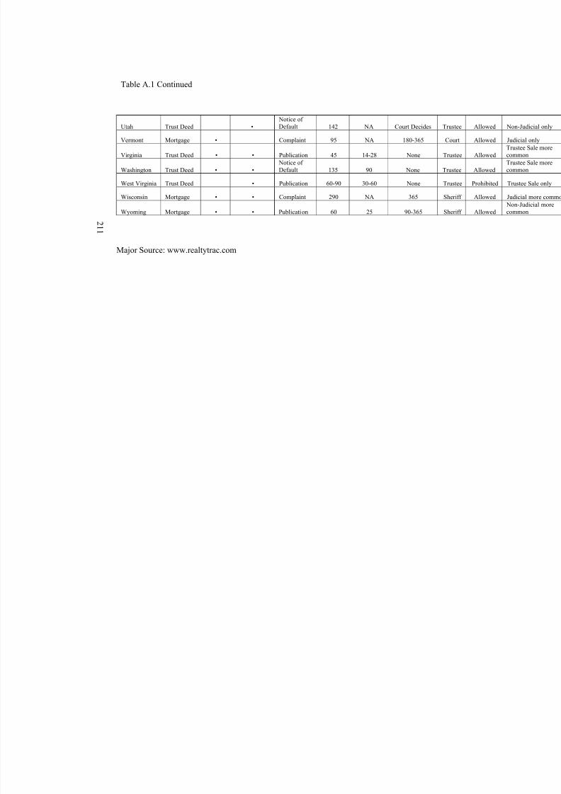
8/6/2019 Spatial Lag Regression
http://slidepdf.com/reader/full/spatial-lag-regression 225/268
2 1 1
Table A.1 Continued
Utah Trust Deed • Notice of Default 142 NA Court Decides Trustee
Vermont Mortgage • Complaint 95 NA 180-365 Court
Virginia Trust Deed • • Publication 45 14-28 None Trustee
Washington Trust Deed • • Notice of Default 135 90 None Trustee
West Virginia Trust Deed • Publication 60-90 30-60 None Trustee
Wisconsin Mortgage • • Complaint 290 NA 365 Sheriff
Wyoming Mortgage • • Publication 60 25 90-365 Sheriff
Major Source: www.realtytrac.com
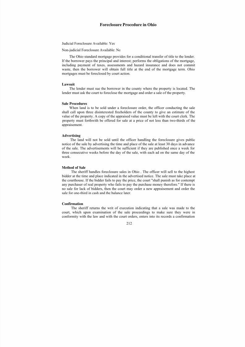
8/6/2019 Spatial Lag Regression
http://slidepdf.com/reader/full/spatial-lag-regression 226/268
212
Foreclosure Procedure in Ohio
Judicial Foreclosure Available: Yes
Non-judicial Foreclosure Available: No
The Ohio standard mortgage provides for a conditional transfer of title to the lender.If the borrower pays the principal and interest; performs the obligations of the mortgage,including payment of taxes, assessments and hazard insurance and does not commitwaste, then the borrower will obtain full title at the end of the mortgage term. Ohiomortgages must be foreclosed by court action.
LawsuitThe lender must sue the borrower in the county where the property is located. The
lender must ask the court to foreclose the mortgage and order a sale of the property.
Sale ProceduresWhen land is to be sold under a foreclosure order, the officer conducting the sale
shall call upon three disinterested freeholders of the county to give an estimate of thevalue of the property. A copy of the appraised value must be left with the court clerk. The property must forthwith be offered for sale at a price of not less than two-thirds of theappraisement.
Advertising
The land will not be sold until the officer handling the foreclosure gives publicnotice of the sale by advertising the time and place of the sale at least 30 days in advanceof the sale. The advertisements will be sufficient if they are published once a week for three consecutive weeks before the day of the sale, with each ad on the same day of theweek.
Method of SaleThe sheriff handles foreclosure sales in Ohio . The officer will sell to the highest
bidder at the time and place indicated in the advertised notice. The sale must take place atthe courthouse. If the bidder fails to pay the price, the court "shall punish as for contemptany purchaser of real property who fails to pay the purchase money therefore." If there is
no sale for lack of bidders, then the court may order a new appraisement and order thesale for one-third in cash and the balance later.
ConfirmationThe sheriff returns the writ of execution indicating that a sale was made to the
court, which upon examination of the sale proceedings to make sure they were inconformity with the law and with the court orders, enters into its records a confirmation
8/6/2019 Spatial Lag Regression
http://slidepdf.com/reader/full/spatial-lag-regression 227/268
213
of the legality of the sale and directs the officer who made the sale to create and deliver the purchaser a deed for the property.
Special ProceduresIf the property is in danger of being damaged the court may appoint a receiver to
take charge of it.
DeficiencyA deficiency judgment may be lender along with the order commanding a
foreclosure sale. The deficiency is void two years after the foreclosure sale is confirmed.However, the enforcement may continue if the debtor signs an agreement to postpone theenforcement past two years.
RedemptionThe debtor can redeem by paying the amount of the judgment plus costs and
interests up until the confirmation of sale, but not afterward.
Source: http://www.defaultresearch.com
8/6/2019 Spatial Lag Regression
http://slidepdf.com/reader/full/spatial-lag-regression 228/268
214
APPENDIX B
TOTAL SHERIFF’S DEEDS AT THE SCHOOL DISTRICT LEVEL INFRANKLIN COUNTY
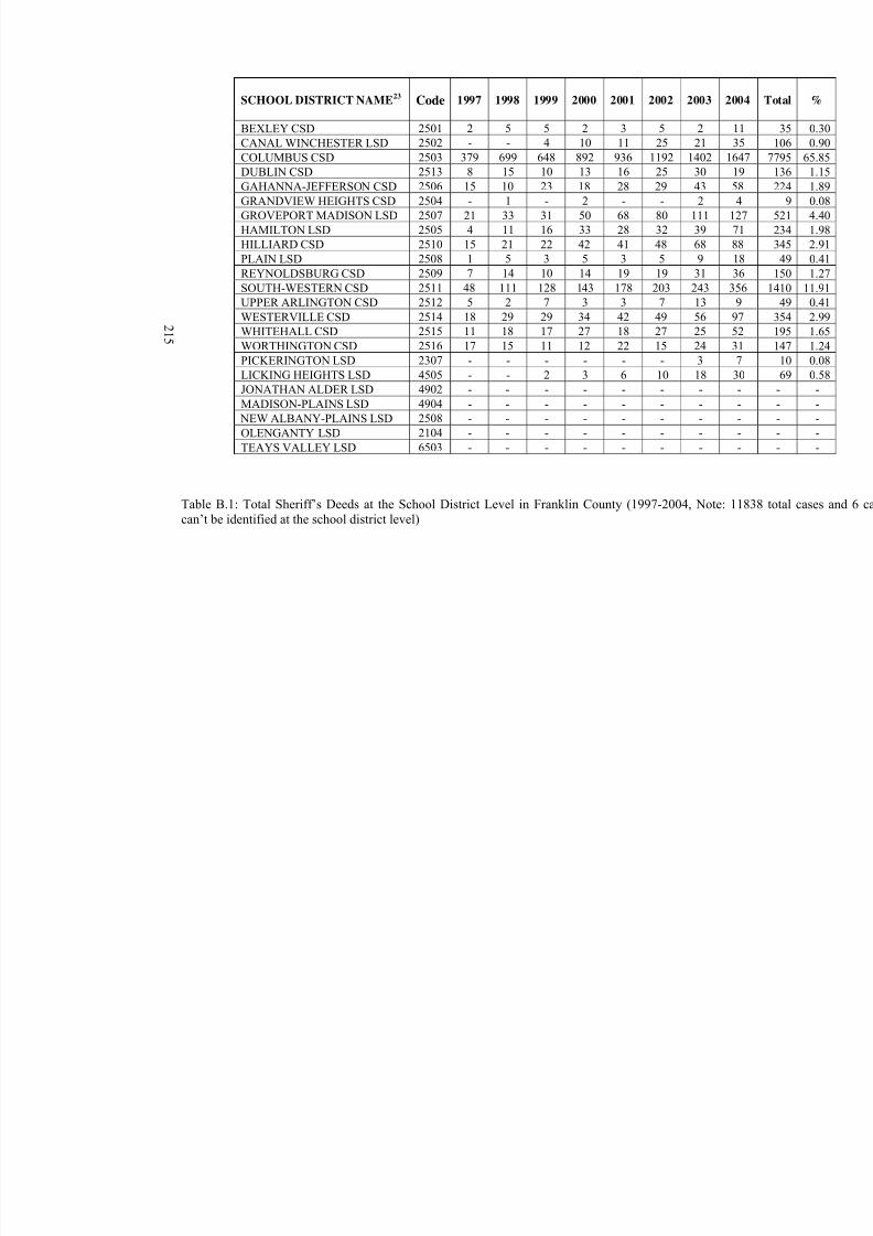
8/6/2019 Spatial Lag Regression
http://slidepdf.com/reader/full/spatial-lag-regression 229/268
2
1 5
SCHOOL DISTRICT NAME23
Code 1997 1998 1999 2000 2001 2002 2003 2
BEXLEY CSD 2501 2 5 5 2 3 5 2
CANAL WINCHESTER LSD 2502 - - 4 10 11 25 21
COLUMBUS CSD 2503 379 699 648 892 936 1192 1402 1
DUBLIN CSD 2513 8 15 10 13 16 25 30
GAHANNA-JEFFERSON CSD 2506 15 10 23 18 28 29 43
GRANDVIEW HEIGHTS CSD 2504 - 1 - 2 - - 2
GROVEPORT MADISON LSD 2507 21 33 31 50 68 80 111
HAMILTON LSD 2505 4 11 16 33 28 32 39
HILLIARD CSD 2510 15 21 22 42 41 48 68
PLAIN LSD 2508 1 5 3 5 3 5 9
REYNOLDSBURG CSD 2509 7 14 10 14 19 19 31
SOUTH-WESTERN CSD 2511 48 111 128 143 178 203 243
UPPER ARLINGTON CSD 2512 5 2 7 3 3 7 13
WESTERVILLE CSD 2514 18 29 29 34 42 49 56
WHITEHALL CSD 2515 11 18 17 27 18 27 25 WORTHINGTON CSD 2516 17 15 11 12 22 15 24
PICKERINGTON LSD 2307 - - - - - - 3
LICKING HEIGHTS LSD 4505 - - 2 3 6 10 18
JONATHAN ALDER LSD 4902 - - - - - - -
MADISON-PLAINS LSD 4904 - - - - - - -
NEW ALBANY-PLAINS LSD 2508 - - - - - - -
OLENGANTY LSD 2104 - - - - - - -
TEAYS VALLEY LSD 6503 - - - - - - -
Table B.1: Total Sheriff’s Deeds at the School District Level in Franklin County (1997-2004, Note: can’t be identified at the school district level)

8/6/2019 Spatial Lag Regression
http://slidepdf.com/reader/full/spatial-lag-regression 230/268
216
APPENDIX C
SPATIAL AUTOCORRELATION OF SELECTED VARIABLES
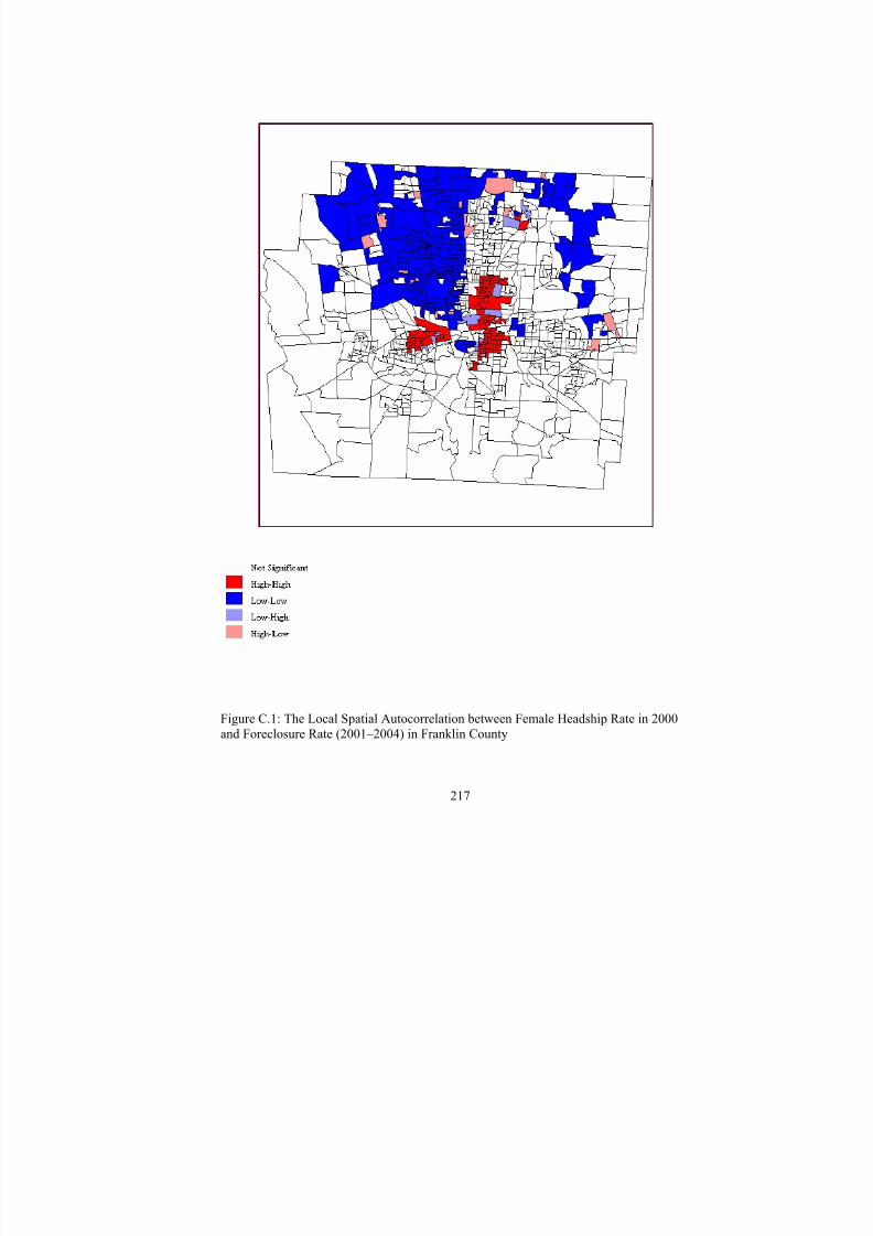
8/6/2019 Spatial Lag Regression
http://slidepdf.com/reader/full/spatial-lag-regression 231/268
217
Figure C.1: The Local Spatial Autocorrelation between Female Headship Rate in 2000and Foreclosure Rate (2001–2004) in Franklin County
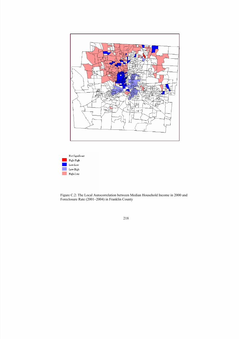
8/6/2019 Spatial Lag Regression
http://slidepdf.com/reader/full/spatial-lag-regression 232/268
218
Figure C.2: The Local Autocorrelation between Median Household Income in 2000 andForeclosure Rate (2001–2004) in Franklin County
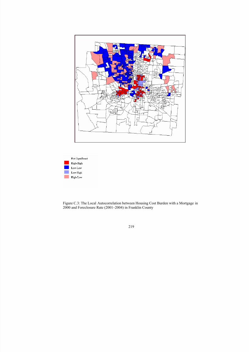
8/6/2019 Spatial Lag Regression
http://slidepdf.com/reader/full/spatial-lag-regression 233/268
219
Figure C.3: The Local Autocorrelation between Housing Cost Burden with a Mortgage in2000 and Foreclosure Rate (2001–2004) in Franklin County
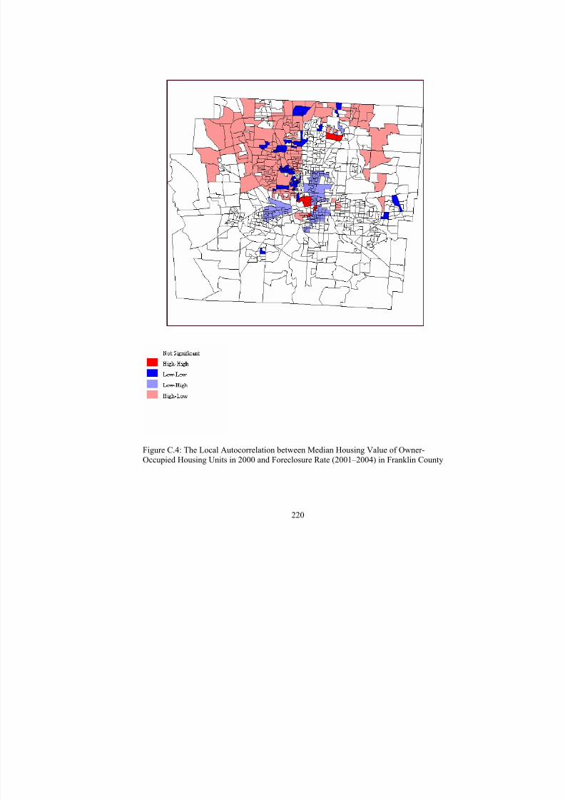
8/6/2019 Spatial Lag Regression
http://slidepdf.com/reader/full/spatial-lag-regression 234/268

8/6/2019 Spatial Lag Regression
http://slidepdf.com/reader/full/spatial-lag-regression 235/268
221
Figure C.5: The Local Autocorrelation between Housing Vacancy Rate in 2000 andForeclosure Rate (2001–2004) in Franklin County
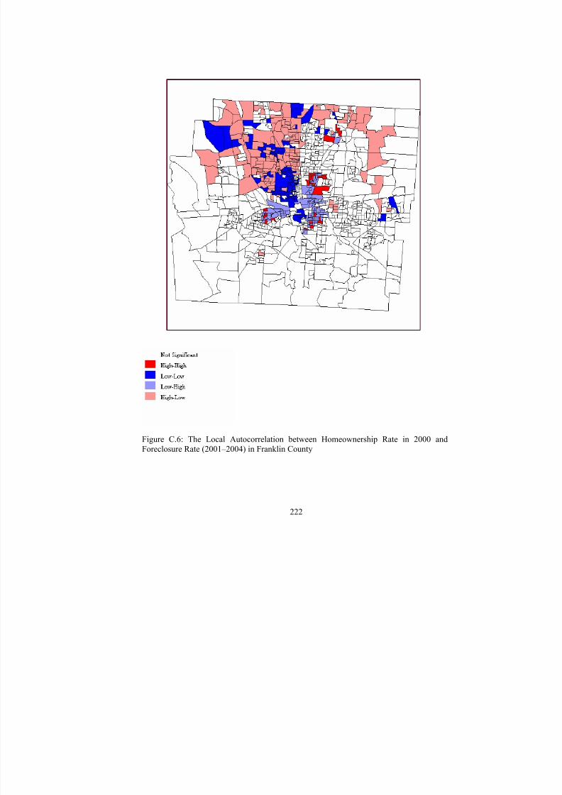
8/6/2019 Spatial Lag Regression
http://slidepdf.com/reader/full/spatial-lag-regression 236/268
222
Figure C.6: The Local Autocorrelation between Homeownership Rate in 2000 andForeclosure Rate (2001–2004) in Franklin County
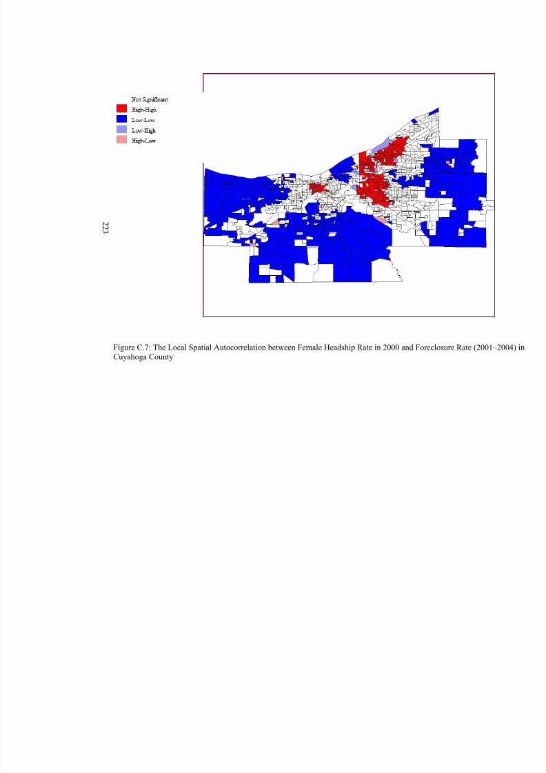
8/6/2019 Spatial Lag Regression
http://slidepdf.com/reader/full/spatial-lag-regression 237/268
2 2 3
Figure C.7: The Local Spatial Autocorrelation between Female Headship Rate in 2000 and Foreclosure RCuyahoga County
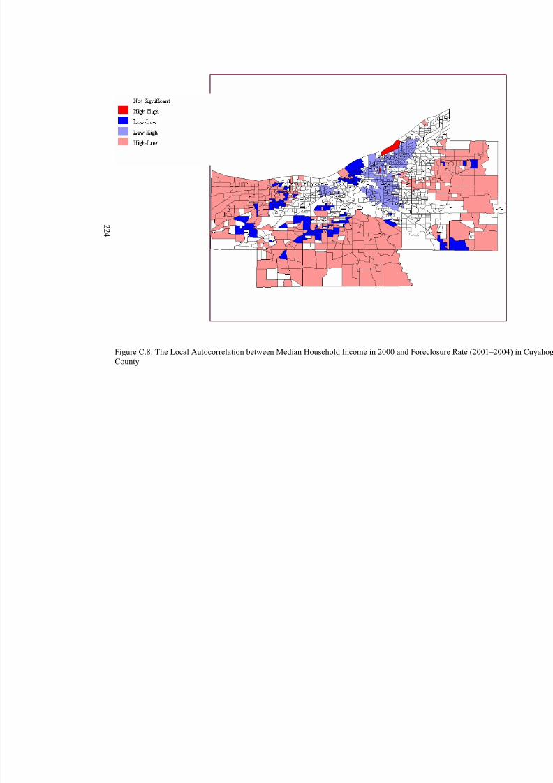
8/6/2019 Spatial Lag Regression
http://slidepdf.com/reader/full/spatial-lag-regression 238/268
2 2 4
Figure C.8: The Local Autocorrelation between Median Household Income in 2000 and Foreclosure RatCounty
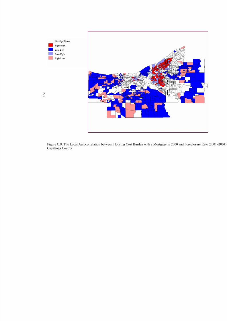
8/6/2019 Spatial Lag Regression
http://slidepdf.com/reader/full/spatial-lag-regression 239/268
2 2 5
Figure C.9: The Local Autocorrelation between Housing Cost Burden with a Mortgage in 2000 and ForeCuyahoga County
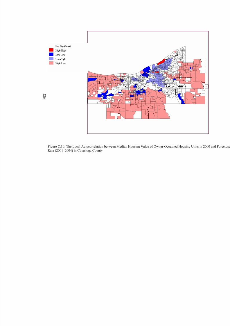
8/6/2019 Spatial Lag Regression
http://slidepdf.com/reader/full/spatial-lag-regression 240/268
2 2 6
Figure C.10: The Local Autocorrelation between Median Housing Value of Owner-Occupied Housing URate (2001–2004) in Cuyahoga County
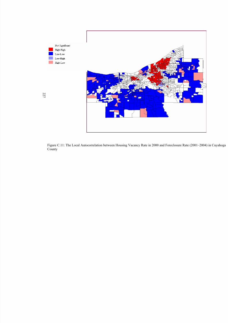
8/6/2019 Spatial Lag Regression
http://slidepdf.com/reader/full/spatial-lag-regression 241/268
2 2 7
Figure C.11: The Local Autocorrelation between Housing Vacancy Rate in 2000 and Foreclosure Rate (2County
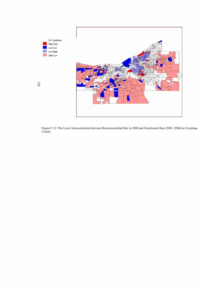
8/6/2019 Spatial Lag Regression
http://slidepdf.com/reader/full/spatial-lag-regression 242/268
2 2 8
Figure C.12: The Local Autocorrelation between Homeownership Rate in 2000 and Foreclosure Rate (20County

8/6/2019 Spatial Lag Regression
http://slidepdf.com/reader/full/spatial-lag-regression 243/268
229
APPENDIX D
SUR MODEL RESULTS
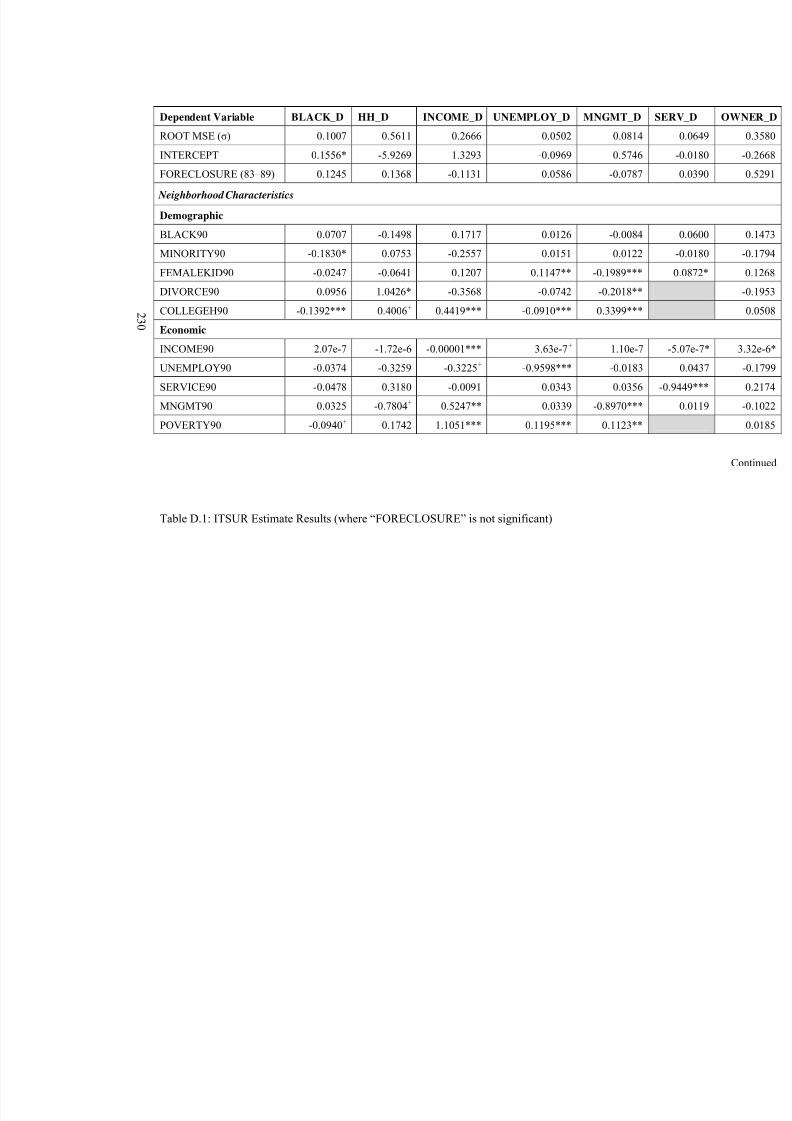
8/6/2019 Spatial Lag Regression
http://slidepdf.com/reader/full/spatial-lag-regression 244/268
2 3 0
Dependent Variable BLACK_D HH_D INCOME_D UNEMPLOY_D MNGMT_D SE
ROOT MSE (σ) 0.1007 0.5611 0.2666 0.0502 0.0814
INTERCEPT 0.1556* -5.9269 1.3293 -0.0969 0.5746
FORECLOSURE (83–89) 0.1245 0.1368 -0.1131 0.0586 -0.0787
Neighborhood Characteristics
Demographic
BLACK90 0.0707 -0.1498 0.1717 0.0126 -0.0084
MINORITY90 -0.1830* 0.0753 -0.2557 0.0151 0.0122
FEMALEKID90 -0.0247 -0.0641 0.1207 0.1147** -0.1989***
DIVORCE90 0.0956 1.0426* -0.3568 -0.0742 -0.2018**
COLLEGEH90 -0.1392*** 0.4006+ 0.4419*** -0.0910*** 0.3399***
Economic
INCOME90 2.07e-7 -1.72e-6 -0.00001*** 3.63e-7+ 1.10e-7
UNEMPLOY90 -0.0374 -0.3259 -0.3225+ -0.9598*** -0.0183
SERVICE90 -0.0478 0.3180 -0.0091 0.0343 0.0356 -
MNGMT90 0.0325 -0.7804+ 0.5247** 0.0339 -0.8970***
POVERTY90 -0.0940+ -0.1742 1.1051*** 0.1195*** 0.1123**
Table D.1: ITSUR Estimate Results (where “FORECLOSURE” is not significant)

8/6/2019 Spatial Lag Regression
http://slidepdf.com/reader/full/spatial-lag-regression 245/268
2 3 1
Table D.1 Continued
Housing
YEARS90 0.0007 -0.0018*** 0.00009+ -0.0001
VALUE90 -2.04e-7 -1.11e-6 1.53e-6*** -9.35e-8 6.75e-7***
VACANCY90 0.2106** 0.2779 -0.0880 0.0967* -0.0002
TENURE90 -0.0666* 0.4421*** -0.0225 0.0016
MORTGAGE90 -0.0284 0.1602 -0.0477 0.0164 -0.0378*
Change in Census Place Characteristics
Demographic
PBLACK_D 1.1124*** -0.2587 -0.0021 0.1003
PCOLL_D -0.4186 1.2331 -0.2124 0.4316
PDIVOR_D -0.4131 0.0930 0.3211 -0.2409
PFEMALE_D -0.2475 0.0448 -0.9977 -0.1725 -0.4667
PHH_D 0.3125 1.6735 0.7695 0.0163 0.0239
Economic
PINC_D -0.0058 -0.3259 -0.0526 0.0936 -0.0136
PUNEMPLOY_D -0.0880 -4.0054 -0.8215 -0.1036 -0.2433

8/6/2019 Spatial Lag Regression
http://slidepdf.com/reader/full/spatial-lag-regression 246/268
2 3 2
Table D.1 Continued
PPOVER_D -0.4732 2.8284 0.1346 -0.0142 0.2956
PMNGMT_D 0.1819* -0.2665 0.2160 -0.0011 0.5423***
PSERV_D 0.1597 -2.1254 -0.3965 0.1749 0.1827
Housing
PTENURE_D 0.4972 1.4083 0.0389 0.2790
POWNER_D -0.3872 1.2556 -0.8065 -0.0338 -0.0899
PVALUE_D 0.0241 0.2966 0.0762 -0.0814 0.0071
PVACAN_D -4.5057 -1.9122 0.3614
*** 0.001 significant level ** 0.01 significant level* 0.05 significant level + 0.10 significant level
8/6/2019 Spatial Lag Regression
http://slidepdf.com/reader/full/spatial-lag-regression 247/268
233
APPENDIX E
THE GEOGRAPHIC DISTRIBUTION OF SELECTED NEIGHBORHOODCHANGE INDICATORS AT THE BLOCK GROUP LEVEL IN FRANKLIN AND
CUYAHOGA COUNTIES
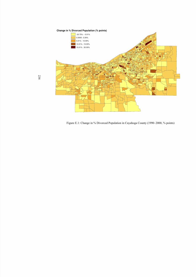
8/6/2019 Spatial Lag Regression
http://slidepdf.com/reader/full/spatial-lag-regression 248/268
2 3 4
Change in % Divorced Population (% points)
-20.75% - -0.01%
0.0000 - 5.00%
5.01% - 10.00%
10.01% - 15.00%
15.01% - 30.00%
Figure E.1: Change in % Divorced Population in Cuyahoga County (1990–2000, %
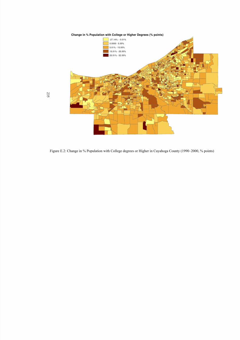
8/6/2019 Spatial Lag Regression
http://slidepdf.com/reader/full/spatial-lag-regression 249/268
2 3 5
Change in % Population with College or Higher Degrees (% points)
-27.14% - -0.01%
0.0000 - 5.00%
5.01% - 15.00%
15.01% - 25.00%
25.01% - 52.00%
Figure E.2: Change in % Population with College degrees or Higher in Cuyahoga County (1990–2000, %
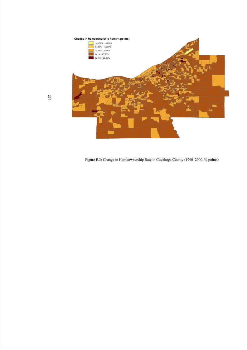
8/6/2019 Spatial Lag Regression
http://slidepdf.com/reader/full/spatial-lag-regression 250/268
2 3 6
Change in Homeownership Rate (% points)
-100.00% - -65.00%
-64.99% - -35.00%
-34.99% - 0.0000
0.01% - 25.00%
25.01% - 55.00%
Figure E.3: Change in Homeownership Rate in Cuyahoga County (1990–2000, %
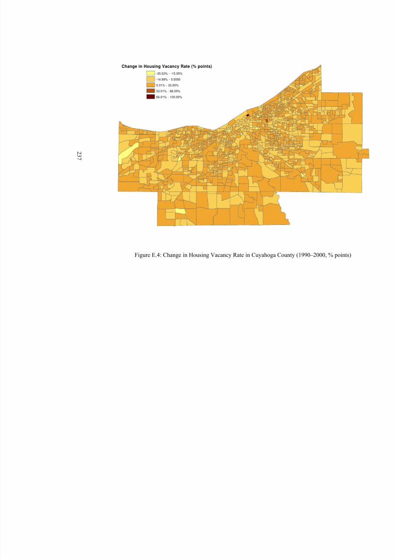
8/6/2019 Spatial Lag Regression
http://slidepdf.com/reader/full/spatial-lag-regression 251/268
2 3 7
Change in Housing Vacancy Rate (% points)
-35.53% - -15.00%-14.99% - 0.0000
0.01% - 33.00%
33.01% - 66.00%
66.01% - 100.00%
Figure E.4: Change in Housing Vacancy Rate in Cuyahoga County (1990–2000, %
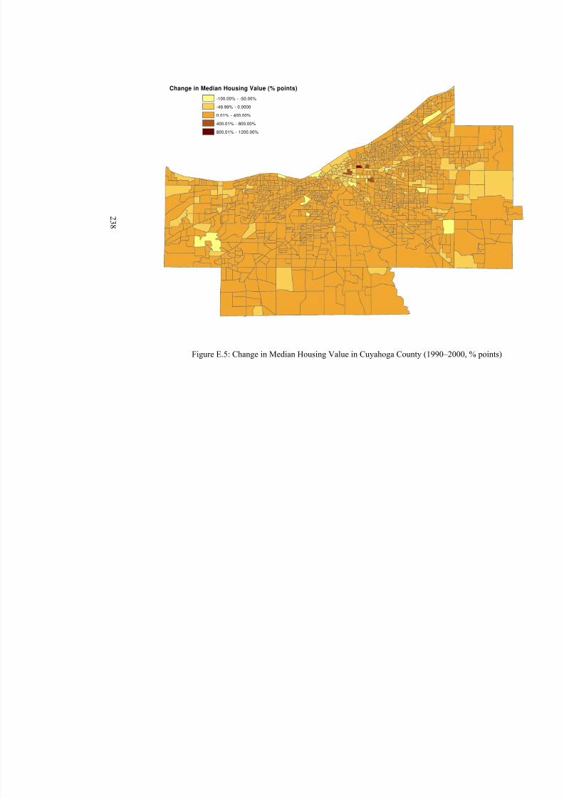
8/6/2019 Spatial Lag Regression
http://slidepdf.com/reader/full/spatial-lag-regression 252/268
2 3 8
Change in Median Housing Value (% points)
-100.00% - -50.00%
-49.99% - 0.0000
0.01% - 400.00%
400.01% - 800.00%
800.01% - 1200.00%
Figure E.5: Change in Median Housing Value in Cuyahoga County (1990–2000, %
8/6/2019 Spatial Lag Regression
http://slidepdf.com/reader/full/spatial-lag-regression 253/268
239
BIBLIOGRAPHY
Ambrose, Brent W. and Charles A. Capone. 2000. The Hazard Rates of the First andSecond Default. Journal of Real Estate Finance and Economics 20(3): 275-293
Ambrose, Brent W., Michael LaCour-Little and Anthony B. Sanders. 2002. Credit
Spreads: Evidence from the Mortgage Market
Ambrose, Brent W. and Anthony B. Sanders. 2003. Commercial Mortgage-Backed
Securities: Prepayment and Default. Journal of Real Estate Finance and Economics 26(2/3): 179-196
Ambrose, Brent W. and Anthony B. Sanders. 2002. High LTV Loans and Credit Risk.Working Paper
Anderson, Richard and James VanderHoff. 1999. Mortgage Default Rates and Borrower Race. Journal of Real Estate Research 18(2): 279-289
Anselin, Luc. 2005. Exploring Spatial Data with Geoda: A Workbook. University of Illinois at Urbana, Champaign
Asher, Herbert B. 1976. Causal Modeling. In Series: Quantitative Applications in the
Social Sciences. Sage Publications
Baku, Esmail and Marc Smith. 1998. Loan Delinquency in Community LendingOrganizations: Case Studies of NeighorWorks Organizations. Housing Policy Debate 9(1): 151-175
Basu, Sabyasachi and Thomas G. Thibodeau. 1998. Analysis of Spatial Autocorrelationin House Prices. The Journal of Real Estate Finance and Economics. 17(1): 61-85
Baxter, Vern and Michey Lauria. 2000. Residential Mortgage Foreclosure and Neighborhood Change. Housing Policy Debate 11(3): 675-699
Bell, Kathleen P. and Nancy E. Bockstael. 2000. Applying the Generalized-MomentsEstimation Approach to Spatial Problems Involving Micro-Level Data. The Review of Economics and Statistics: 82(1):72-82
8/6/2019 Spatial Lag Regression
http://slidepdf.com/reader/full/spatial-lag-regression 254/268
240
Berkovec, J., G. Canner, S. Gabriel, and T. Hannan. 1994. Race, Redlining, andResidential Mortgage Loan Performance. Journal of Real Estate Finance and Economics 9:263–294.
______. 1995. Discrimination, Default, and Loss in FHA Mortgage Lending. Paper
presented at the American Real Estate and Urban Economics Association AnnualMeeting.
Berry, William D. 1984. Nonrecursive Causal Models. Sage Publications
Bollen, Kenneth A. 1989. Structural Equations with Latent Variables. New York: Wiley
Bunce, Harold L., William J. Reeder and Randall M. Scheessele. 1999. UnderstandingConsumer Credit and Mortgage Scoring: A Work in Progress at HUD. UnpublishedPaper. The U.S. Department of Housing and Urban Development
Bradbury, Katherine L., Anthony Downs, and Kenneth A. Small. 1982. Urban Declineand the Future of American Cities. Washington D.C.: Brookings Institution
Brooks-Gunn, Jeanne, Gred J. Duncan, and J. Lawrence Abner, eds. 1997. Neighborhood
Poverty: Context and Consequences for Children. Volume I. New York: Russell SageFoundation.
Calhoun, Charles A. and Yongheng Deng, 2002. A Dynamic Analysis of Fixed- andAdjustable-Rate Mortgage Terminations. Journal of Real Estate Finance and Economics 24: 9-33
Can, Ayse. 1996. Spatial Segmentation in Urban House Prices: Alternative Approaches.Washington DC. Fannie Mae Foundation. Mimeo.
Can, Ayse. 1992a. Residential Quality Assessment: Alternative Approaches Using GIS.The Annals of Regional Science 26: 97-110
Can, Ayse. 1992b. Specification and Estimation of Hedonic Housing Price Models. Regional Science and Urban Economics 22: 453-474
Can, Ayse, and Isaac Megbolugbe, 1997. Spatial Dependence and House Price IndexConstruction, Journal of Real Estate Finance and Economics 32: 2214-2232
Can, Ayse. 1998. GIS and Spatial Análysis of Housing and Mortgage Market. Journal of Housing Research 9(1): 61-86
Capone, Charles A. Jr. et. al. 1996. Providing Alternatives to Mortgage Foreclosure: AReport to Congress. U.S. Department of Housing and Urban Development
8/6/2019 Spatial Lag Regression
http://slidepdf.com/reader/full/spatial-lag-regression 255/268
241
Carroll, Thomas M., Terrence M. Clauretie and Helen R. Neil. 1995. Effect of Foreclosure Status on Residential Selling Price: Comment. Journal of Real Estate
Research
Carroll, Thomas M., Terrence M. Clauretie, Helen Neil and Cindy Jorgensen. 1995. HUD
versus Private Bank Foreclosures: A Spatial and Temporal Analysis. Journal of Housing Economics 4: 183-194
Case, Karl E and Maryna Marynchenko. 2001. Home Price Appreciation in Low- andModerate-Income Markets. Joint Center for Housing Studies, Harvard University.Presented at the Symposium on Low-Income Homeownership as an Asset-BuildingStrategy.
Carter, William H., Michael H. Schill, and Susan M. Wachter. 1998. Polarization, PublicHousing, and Racial Minorities in U.S. Cities. Urban Studies 35(10):1889-911
Case, Karl and Robert Shiller. 1994. A Decade of Boom and Bust in the Prices of Single-Family Homes: Boston and Los Angeles: 1983-1993. New England Economic Review:40-51.
______. 1996. Mortgage Default Risk and Real Estate Prices: The Use of Index-basedFutures and Options in Real Estate. Journal of Housing Research 7(2): 243-258
Cincotta, Gale, David Rose, and Liz Ryan. 1998. The Devil’s in the Details: An Analysisof Federal Housing Administration Default Concentration and Lender Performance in 20U.S. Cities. Chicago: National Training and Information Center
Clark, W.A.V. 1992. Residential Preferences and Residential Choices in a MultiethnicContext. Demography 29: 451-466
Clauretie, Terrence M. 1987. The Impact of Interstate Foreclosure Cost Differences andthe Value of Mortgages on Default Rates. AREUEA (American Real Estate and Urban
Economics Association) Journal 15(3): 152-67
Cook, Christine C. 1988. Components of Neighborhood Satisfaction: Responses fromUrban and Suburban Low-Income, Single-Parent Women. Environment and Behavior 20(2): 115-149
Cotterman, Robert F. 2001. Neighborhood Effects in Mortgage Default Risk. Preparedfor the Office of Policy Development and Research. The U.S. Department of Housingand Urban Development
______. 2002. New Evidence on the Relationship between Race and Mortgage Default:The Importance of Credit History Data. Study Prepared for the Office of PolicyDevelopment and Research. The U.S. Department of Housing and Urban Development

8/6/2019 Spatial Lag Regression
http://slidepdf.com/reader/full/spatial-lag-regression 256/268
242
______. 2003. Assessing Problems of Default in Local Mortgage Market. Prepared for the Office of Policy Development and Research, U.S. Department of Housing and UrbanDevelopment
______. 2004. Analysis of FHA Single-Family Default and Loss Rate. Prepared for the
Office of Policy Development and Research, U.S. Department of Housing and UrbanDevelopment
Coulson, N. Edward and Eric W. Bond. 1990. A Hedonic Approach to ResidentialSuccession. The Review of Economics and Statistics 72(3): 433-44
CRL (Center for Responsible Lending). 2004. Predatory Mortgage Lending: A Women’sIssue. CRL Issue Brief 15
Crowder, Kyle. 2000. The Racial Context of White Mobility: An Individual LevelAssessment of the White Flight Hypothesis. Social Science Research 29:223-257
Deng, Yongheng and Stuart Gabriel, 2002. Modeling the Performance of FHA-InsuredLoans: Borrower Heterogeneity and the Exercise of Mortgage Default and PrepaymentOptions, Prepared for the Office of Policy Development and Research, The U.S.Department of Housing and Urban Development
______. 2003. Are Underserved Borrowers Lower Risk? New Evidence on thePerformance and Pricing of FHA-Insured Mortgages. University of Southern California
Denton, Nancy A. and Douglas S. Massey. 1991. Patterns of Neighborhood Transition ina Multiethnic World: U.S. Metropolitan Areas, 1970-1980. Demography 28(1): 41-63
Dietz, Robert. 2002. Estimation of Neighborhood Effects in the Social Sciences: AnInterdisciplinary Approach. Social Science Research 31(4):539-575
Downs, Anthony. 1981. Neighborhood and Urban Development . Washington D.C.:Brookings Institution
Duncan, Otis D. and Beverly Duncan. 1957. The Negro Population of Chicago. Chicago,IL: University of Chicago Press
Eggers, Mitchell L., and Douglas Massey. 1992. A Longitudinal Analysis of UrbanPoverty: Blacks in U.S. Metropolitan Areas between 1970 and 1980. Social ScienceResearch 21(2): 175-203
Ellen, Ingrid Gould. 2000. Sharing the America’s Neighborhoods: The Prospects for Stable Racial Integration. Cambridge, MA: Harvard University Press
8/6/2019 Spatial Lag Regression
http://slidepdf.com/reader/full/spatial-lag-regression 257/268
243
Elwakil, Mohamed Abdel-Washed. 1994. Identifying and Predicting Changes in Neighborhood Quality: Experiments in Techniques to Assess Quality and ProjectChange. Dissertation: The Ohio State University
Faris, Robert. 1967. Chicago Sociology 1920-1932. Chicago: University of Chicago
Press
Farley, Reynolds, et.al. 1994. Stereotypes and Segregation: Neighborhoods in the DetroitArea. American Journal of Sociology 100(3): 750-780
Flippen, Chenoa A. 2001. Racial and Ethnic Inequality in Homeownership and HousingEquity. Sociological Quarterly 42: 121-149
Forgarty, Michael S. 1977. Predicting Neighborhood Decline within a Large CentralCity: An Application of Discriminant Analysis. Environment and Planning 9:579-84
Forgey, F.A., R.C. Rutherford and M. L. VanBuskirk. 1994. Effect of Foreclosure Statuson Residential Selling Price. Journal of Real Estate Research 9(3): 313-318
Foster, Chester and Robert Van Order. 1985. An Option-based Model of MortgageDefault. Housing Finance Review 3(3): 273-291
Frumkin, Norman. 2000. Guide to Economic Indicators (Third Edition). M.E. Shape Inc.
Galster, George C. 1990. White Flight from Racially Integrated Neighborhoods in the1970s: The Cleveland Experience. Urban Studies 27(3): 385-399
Galster, George C., and Ed. Hill. 1992. The Metropolis in Black and White. NewBrunswick, NJ: Center for Urban Policy Research
Galster, George C. and Ronald Mincy. 1993. Understanding the Changing Fortunes of Metropolitan Neighborhoods. Housing Policy Debate 4(3):303-52
Galster, George C., Ronald B. Mincy, and Mitchell S. Tobin. 1997. The Disparate Racial Neighborhood Impacts of Metropolitan Economic Restructuring. Urban Affairs Review 32(6): 797-824
Galster, George C. 2003. Neighborhood Dynamics and Housing Markets. In TonyO’Sullivan and Kenneth Gibb (eds.). Housing Economics & Public Policy: 153-71.Oxford, UK: Blackwell Publishing
Galster, George C., Roberto G. Quercia and Alvaro Corte. 2000. Identifying Neighborhood Thresholds: An Empirical Exploration. Housing Policy Debate 11(2): 701-32
8/6/2019 Spatial Lag Regression
http://slidepdf.com/reader/full/spatial-lag-regression 258/268
244
Galster, George C. and Jackie M. Krall. 2003. Exploring Endogenous NeighborhoodDynamics. Paper presented at the ACSP/AESOP conferences
Goering, John and Ron Wienk (ed.). 1996. Mortgage Lending, Racial Discrimination and
Federal Policy. The Urban Institute Press. Washington D.C.
Goldstein, Ira. 2004. Bringing Subprime Mortgages to Market and the Effects on Lower-Income Borrowers. Joint Center for Housing Studies. Harvard University
Grant, Donald E. 1995. The Political Economy of Business Failures across the AmericanStates. American Sociological Review 60(6):851-873
Grigsby, William G., Morton Baratz, George Galster, and Duncan Maclenna. 1987. TheDynamics of Neighborhood Change and Decline. Progress in Planning 28:1-76
Guest, Avery M. 1972. Urban History, Population Densities, and Higher Status
Residential Location. Economic Geography 48:375-87
Guest, Avery M. 1973. Urban Growth and Population Densities. Demography 10(1):53-69
Guest, Avery M. 1974. Neighborhood Life Cycles and Social Status. EconomicGeography 50: 228-43
Guest, Avery M. and James A. Weed. 1976. Ethnic Residential Segregation: Patterns of Change. American Journal of Sociology 81(5):1088-111
Harris, David R. 1999. Property Value Drop When Blacks Move In Because…” Racialand SES Determinants of Neighborhood Quality. American Sociological Review 64: 461-479
Harrison, Ben, and Barry Bluestone. 1988. The Great U-Turn. New York: Basic
Hartarska, Valentina, Claudio Gonzalez-Vega and David Dobos. 2002. Credit Counselingand the Incidence of Default on Housing Loans by Low-Income Households. RuralFinance Program. The Ohio State University
Harvey, David. 1973. Social Justice and the City. Oxford, England: Blackwell
Herzog, J.P., and J.S. Earley. 1970. Home Mortgage Delinquency and Foreclosure. NewYork: National Bureau of Economic Research
Hoover, Edgar M. and Raymond Vernon. 1959. Anatomy of a Metropolis. Cambridge,MA: Harvard University Press
8/6/2019 Spatial Lag Regression
http://slidepdf.com/reader/full/spatial-lag-regression 259/268
245
HUD (The U.S. Housing and Urban Development Department). 1986. Providing
Alternatives to Foreclosure: A Report to Congress
______. 1992. Report to Congress on the Home Loan Mortgage Corporation: 120-176
______. 2004. Housing Goals for Fannie Mae and Freddie Mac for the Years 2005-2008:Chapter VI: Costs of Housing Goals: Credit Risk.
IMBA (Indiana Mortgage Bankers Association). 2003. Indiana Mortgage Foreclosure
Rate
Immergluck, Dan, and Geoff Smith. Measuring Neighborhood Diversity and Stability inHome-Buying: Examining Patterns by Race and Income in a Robust Housing Market.Journal of Urban Affairs 25(4): 473-491
Immergluck, Dan, and Geoff Smith. 2005a. The External Costs of Foreclosure: The
Impact of Single-Family Foreclosures on Property Values.
Immergluck, Dan, and Geoff Smith. 2005b. The Impact of Single Family MortgageForeclosures on Neighborhood Crime.
Jargowsky, Paul. 1997. Poverty and Place. New York: Russell Sage
Johnston, John. 1984. Econometric Methods, 3rd ed. New York, NY: McGraw-Hill
Jung, A. 1962. Terms on Conventional Mortgage Loans on Existing Homes. Journal of
Finance 17: 432-443
Kiel, Katherine A. 1994. The Impact of House Price Appreciation on HouseholdMobility. Journal of Housing Economics 3:92-108
Kline, Rex B. 1998. Structural Equation Modeling. New York, NY: The Guilford Press
Krivo, Lauren J., Ruth D. Peterson, Helen Rizzo, and John R. Reynolds. 1998. Race,Segregation, and the Concentration of Disadvantage: 1980-1990. Social Problems 45(1):61-80
LaCour-Little, Michael and Richard K. Green. 1998. Are Minorities or Minority Neighborhoods More Likely to Get Low Appraisals? Journal of Real Estate Finance and
Economics 16(3): 301-315
LaCour-Little, Michael. 2004. Equity Dilution: An Alternative Perspective on MortgageDefault. Real Estate Economics 32(3):359-384
8/6/2019 Spatial Lag Regression
http://slidepdf.com/reader/full/spatial-lag-regression 260/268
246
LaCour-Little, Michael and Stephen Malpezzi. 2003. Appraisal Quality and ResidentialMortgage Default: Evidence from Alaska. Journal of Real Estate Finance and Economics 27(2):211-233
Lauria, Mickey. 1998. A New Model of Neighborhood Change: Reconsidering the Role
of White Flight. Housing Policy Debate 9(2): 395-424
Lauria, Mickey and Vern Baxter. 1999. Residential Mortgage Foreclosure and RacialTransition in New Orleans. Urban Affairs Review 34(6): 757-786
Lauria, Mickey, Vern Baxter and Bridget Bordelon. 2004. An Investigation of the Time between Mortgage Default and Foreclosure. Housing Studies 19(4): 581-600
Lin, Emily Y. and Michelle J. White. 2001. Bankruptcy and the Market for Mortgage andHome Improvement Loans. Journal of Urban Economics 50: 138-162
Logan, John, and Harvey Molotch. 1987. Urban Fortunes: The Political Economy of Place. Berkeley, CA: University of California Press
Maclennan, Duncan. 1982. Housing Economics: An Applied Approach. London,UK:Longmans
Manski, Charles F. 1993. Identification of Endogenous Social Effects: The ReflectionProblem. Review of Economic Studies 60: 531-542
Manski, Charles F. 2000. Economic Analysis of Social Interactions. Journal of Economic
Perspectives
Massey, Douglas S. , and Nancy A. Denton. 1993. American Apartheid: Segregation andthe Making of the Underclass. Cambridge, MA: Harvard University Press.
Massey, Douglas S. 1990. American Apartheid: Segregation and the Making of theUnderclass. American Journal of Sociology 96:329-357
Massey, Douglas S., and Mitchell L. Eggers. 1990. The Ecology of Inequality: Minoritiesand the Concentration of Poverty, 1970-1980. American Journal of Sociology95(5):1153-1188
Massey, Douglas S. and Nancy A. Denton. 1993. American Apartheird: Segregation and
the Making of the Underclass. Cambridge: Harvard University Press
Moffitt, Robert A. 2000. Welfare Benefits and Female headship in U.S. Time Series.John Hopkins University
Muth, Richard F. 1969. Cities and Housing. Chicago: University of Chicago Press
8/6/2019 Spatial Lag Regression
http://slidepdf.com/reader/full/spatial-lag-regression 261/268
247
Noordewier, Thomas G., David M. Harrison and K. Ramagopal. 2001. Semivariance of Property Value Estimates as a Determinant of Default Risk. Real Estate Economics 29(1): 127- 159
OCC(Comptroller of the Currency). 2003. Economic Issues in Predatory Lending. OCC
Working Paper
Odland, John. 1988. Spatial Autocorrelation. Sage Publications, Inc. CA: Newbury Park
Oliver, M, and T. Shapiro. 1995. Black Wealth / White Wealth: A New Perspective on
Racial Inequality. New York: Routledge.
Pace, R. Kelley, Ronald Barry and C. F. Sirmans. 1998. Spatial Statistics and Real Estate.The Journal of Real Estate Finance and Economics: 17(1):5-13
Page, A. 1964. The Variation of Mortgage Interest Rates. Journal of Business 37(3): 280-
294
Pavlov, Andrey D. 2001. Competing Risk of Mortgage Termination: Who Refinances,Who Moves, and Who Defaults? Journal of Real Estate Finance and Economics 23(2):185-211
Park, Robert A. 1952. Human Communities. Glencoe, IL: Free Press
Pennington-Cross, Anthony. 2003. Credit History and the Performance of Prime and Nonprime Mortgages. Journal of Real Estate Finance and Economics 27(3): 279-301
______. 2003. The Value of Foreclosed Property: House Prices, Foreclosure Laws, andAppraisals. Office of Federal Housing Enterprise and Oversight
Pence, Karen M. 2003. Foreclosing on Opportunity: State Laws and Mortgage Credit.Board of the Governors of the Federal Reserve System
Phillips, Richard A. and James H. VanderHoff. 2004. The Conditional Probability of Foreclosure: An Empirical Analysis of Conventional Mortgage Loan Defaults. Real
Estate Economics 32(4): 571-587
OCI (The Ohio Continuing Legal Education Institute). 1996. Foreclosure Practice. OhioCLE Institute
Ottensmann, John R. and Michael E. Gleeson. 1992. The Movement of Whites andBlacks into Racially Mixed Neighborhoods: Chicago, 1960-1980. Social ScienceQuarterly 73(3): 645-62
Ottensmann, John R., David H. Good, and Michael E. Gleeson. 1990. The Impact of NetMigration on Neighborhood Racial Composition. Urban Studies 27(5):705-17
8/6/2019 Spatial Lag Regression
http://slidepdf.com/reader/full/spatial-lag-regression 262/268
248
Pindyck, Robert S. and Daniel L. Rubinfeld. 1991. Econometric Models and Economic
Forecast . 3rd. ed. McGraw-Hill, Inc.
Quercia, Roberto G., and Michael A. Stegman. 1992, Residential Mortgage Default: A
Review of the Literature. Journal of Housing Research. Vol 3 (2): 341-379
Quercia, Robert G., George W. McCarthy and Michael S. Stegman. 1995. MortgageDefault among Rural, Low-Income Borrowers. Journal of Housing Research 6(2): 349-369
Quercia, Roberto G. and George C. Galster. 1997. Threshold Effects and the ExpectedBenefits of Attracting Middle Income Households to the Central City. Housing Policy
Debate 8(2):409-35
Quercia, Roberto G., Spencer M. Cowan and Ana Moreno. 2004. The Cost-Effectiveness
of Community-based Foreclosure Prevention. Joint Center for Housing Studies. HarvardUniverseity
Quercia, Roberto G. et. al. 2000. Spatial-Temporal Measurement of House PriceAppreciation in Under Served Areas. Journal of Housing Research. Volume 11. Issue 1.
Quercia, Roberto G. and George C. Galster. 2000. Threshold Effects and NeighborhoodChange. Journal of Planning Education and Research 20:146-62
Quigley, John, Robert Van Order and Yongheng Deng. 1993. The Competing Risks for Mortgage Termination by Default and Prepayment in Residential Housing Markets.Paper Presented at the NBER Summer Institute. Cambridge, Mass.
Raffalovich, Lawrence. et. al. 2002. Racial Disparities in Housing Value Appreciation:Six Metropolitan Areas, 1980-1990. Presented at the 97 th Annual Meetings of theAmerican Sociological Association.
Realtors (National Association of Realtors) Research Division. 2003. Rising Foreclosure
Rates in Indiana: An Explanatory Analysis of Contributing Factors.
Rhey Richard and Ari Posner. 2004. The American Dream Lost: Foreclosures in Pima
County, Arizona. Prepared for Pima County Community Development and NeighborhoodConservation Department
Ross, Stephen L. 1996. Flaws in the Use of Loan Defaults to Test for Mortgage LendingDiscrimination. CityScape: A Journal of Policy Development and Research 2(1): 41-48.The U.S. Department of Housing and Urban Development
8/6/2019 Spatial Lag Regression
http://slidepdf.com/reader/full/spatial-lag-regression 263/268
249
Rothenburg, Jerome, George Galster, Richard Butler, and John Pitkin. 1991. The Maze of
Urban Housing Markets: Theory, Practice, and Evidence. Chicago, IL: University of Chicago Press
Sandor, R., and H. Sosin. 1975. The Determinants of Mortgage Risk Premiums: A Case
Study of the Portfolio of a Savings and Loan Association. The Journal of Business 48(1):27-38
Saunders, Anthony and Marcia Millon Cornett. 2003. Financial Institutions
Management: A Risk Management Approach. 4th Edition. McGraw-Hill, Irwin: 259-322
Schelling, Thomas C. 1971. Dynamic Models of Segregation. Journal of Mathematical
Sociology 1: 143-86
Schelling, Thomas C. 1972. The Process of Residential Segregation: NeighborhoodTipping. In Anthony H. Pascal (ed.). Racial Discrimination in Economic Life, 157-84.
Lexington, MA: D.C., Heath and Co.
Schwab, W. A. and E. Marsh. 1980. The Tipping-Point Model: Prediction of Change inthe Racial Composition of Cleveland, Ohio, Neighborhoods, 1940-1970. Environment
and Planning A 12: 385-98
Schwirian, Kent. 1983. Models of Neighborhood Change. Annual Review of Sociology 9:83-102
Shapiro, T. 2004. The Hidden Cost of Being African American: How Wealth Perpetuates
Inequality: Oxford University Press.
South, Scott, and Kyle D. Crowder. 1997. Escaping Distressed Neighborhoods:Individual, Community, and Metropolitan Influences. American Journal of Sociology102(4): 1040-1084
Squires, Gregory D. 1994. Capital and Communities in Black and White. Albany, NY:State University of New York.
Stegman, Michael A, Roberto G. Quercia, and Walter R. Davis. 2003. NC’s Anti-Predatory Lending Law: Doing What it’s Supposed to Do: A Reply. Center for Community Capitalism. University of North Carolina at Chapel Hill
Stock, Richard D., et.al. 2001. Predation in the Sub-prime Lending Market: MontgomeryCounty. Prepared for Lutheran Social Services of the Miami Valley
Stone, Michael E. 1986. Housing and the Dynamics of U.S. Capitalism. In CriticalPerspectives on Housing, ed. Rachel G. Bratt, Chester Hartman, and Anne Meyerson, 41-67. Philadelphia: Temple University Press
8/6/2019 Spatial Lag Regression
http://slidepdf.com/reader/full/spatial-lag-regression 264/268
8/6/2019 Spatial Lag Regression
http://slidepdf.com/reader/full/spatial-lag-regression 265/268
251
Young, H. Peyton. 1998. Individual Strategy and Social Structure: An Evolutionary
Theory of Institutions. Princeton, NJ: Princeton University Press
Zellner, Arnold. 1962. An Efficient Method of Estimating Seemingly Unrelated
Regressions and Tests of Aggregation Bias. Journal of the American Statistical Association 57:500-509.
Zhang, J. 2001. Racial Segregation in an All-Integrationist World . San Francisco, CA:Public Policy Institute of California
8/6/2019 Spatial Lag Regression
http://slidepdf.com/reader/full/spatial-lag-regression 266/268
252
NOTES
1 Burnout means the tendency of mortgage pools in mortgage-related securities to become less sensitive tointerest rate as they tend to maturity. The older the pool, the more burnt out is the sensitivity to interest ratechanges. In a burnout refinancing the mortgage will not bring more benefits than before the burnout, thusthe borrowers missed previous good opportunities to refinance and have a higher tendency to default.
2 As suggested by Burridge (1980), the Largange Multiplier principle can be applied for the test for spatialerror dependence can be based on. The test is:
)(/)( 22
'
W W W tr W e
error LM e +′=− σ
where tr represents the matrix trace operator, σ2 is a maximum likelihood estimate for the error variance
(i.e., σ2=e’e/N). The LM-error follows an asymptotic χ2(1) distribution under the null hypothesis of no
spatial dependence (H0: λ=0).
3 To test for the substantive spatial dependence, Anselin (1988) suggested an alternative LargrangeMultiplier test:
⎥⎦
⎤⎢⎣
⎡ +′+′′
=− )()(
/ 2
22W W W tr
MWXbWXbWyelag LM
σ σ
where Wy is the spatial lag, b is vector of the OLS estimators for parameters β, M is a projection matrix,
M=I-X(X’X)-1X’. The LM-lag also follows an asymptotic χ2(1) distribution under the null hypothesis of
no spatial dependence (H0: ρ=0).
4 The robust LM tests are robust to misspecification of the other source of spatial dependence—i.e. therobust LM error test is robust to any spatial lag dependence that may be present and vice versa (i.e. tests for error dependence in presence of missing lag), the robust LM lag test is robust to any spatial error dependence that may be present (tests for lag dependence in presence of missing error).
5 The 1990 Median Household Income has been converted to the 2000 constant dollar values based on thedeflator.
6 The Median Housing Value of owner-occupied housing units has been converted to the 2000 constantdollar values based on the deflator.
7
Among the available parcel datasets (1988, 1994, 1997, 2000, 2004), 1988 Cuyahoga Parcel data are theclosest to capture most of the 9,185 Sheriff’s Deeds in 1983–1989.
8 The Median Household Income has been converted to the 2000 constant dollar values based on thedeflator.
9 The Median Housing Value of owner-occupied housing units has been converted to the 2000 constantdollar values based on the deflator.
10 The foreclosure data in this time period are not available in Franklin County.
8/6/2019 Spatial Lag Regression
http://slidepdf.com/reader/full/spatial-lag-regression 267/268
253
11 Heteroskedasticity-Robust OLS adjustment is used to correct for heteroskedasticity in the OLSregression, base on White’s standard errors. Heteroskedasticity-robust (H-Robust) standard errors are very popular in applied econometrics, and in practice they are more often used to deal with heteroskedasticitythan Weighted Least Squares. Please refer to textbooks in econometrics for detailed procedures of
conducting the adjustments.12 R 2 in a spatial model is called Pseudo R-square, which is defined as the ratio of the variance of the predicted values over the variance of the observed values for the dependent variable. Therefore it is notdirectly comparable with the results from the OLS regression. Log Likelihood is appropriately comparable between spatial models and OLS models.
13 Please refer to Spatial Econometrics: Methods and Models (Luc Anselin, 1989) for the detailed statisticdescription of the log likelihood functions in spatial models.
14 The Jarque-Bera test is a goodness-of-fit measure of departure from normality, based on the samplekurtosis and skewness. The test statistic JB is defined as
)4
)3((6
)( 22 −+−= K Sk n JB
where S is the skewness, K is the kurtosis, n is the number of observations, and k is the number of estimatedcoefficients used to create the series. The statistic has an asymptotic chi-squared distribution with twodegrees of freedom and can be used to test the null hypothesis that the data are from a normal distribution;since samples from a normal distribution have an expected skewness of 0 and an expected kurtosis of 3. Asthe equation shows, any deviation from this increases the JB statistic.
15 The first step of Breusch-Pagan test is to obtain the residuals of the estimated regression equation. Thenuse the squared residuals as the dependent variable in a secondary equation that includes all theindependent variables suspected of being related to the error term:
i pi pii Z Z e μ α α α ++++= L1102)( .
Afterwards use a Chi-square test to test that all the coefficients in this equation are zero.
16 As in a Breusch-Pagan test the first step of White test is to obtain the residuals of the estimatedregression equation. Then use the squared residuals as the dependent variable in a secondary equation thatincludes all the independent variables from the original regression equation:
i pi pii X X e μ α α α ++++= L1102)(
Afterwards use a Chi-square test to test that all the coefficients in this equation are zero.
17 Please refer to Spatial Econometrics: Methods and Models (Luc Anselin, 1989) for the detailed statisticdescription of the log likelihood functions in spatial models.
18 The Jarque-Bera test is a goodness-of-fit measure of departure from normality, based on the samplekurtosis and skewness. The test statistic JB is defined as
)4
)3((
6
)( 22 −+
−=
K S
k n JB
where S is the skewness, K is the kurtosis, n is the number of observations, and k is the number of estimatedcoefficients used to create the series. The statistic has an asymptotic chi-squared distribution with two
8/6/2019 Spatial Lag Regression
http://slidepdf.com/reader/full/spatial-lag-regression 268/268
degrees of freedom and can be used to test the null hypothesis that the data are from a normal distribution;since samples from a normal distribution have an expected skewness of 0 and an expected kurtosis of 3. Asthe equation shows, any deviation from this increases the JB statistic.