Spatial Input-Output Models: PECAS · PDF fileSpatial Input-Output Models: PECAS Webinar 4 of...
93
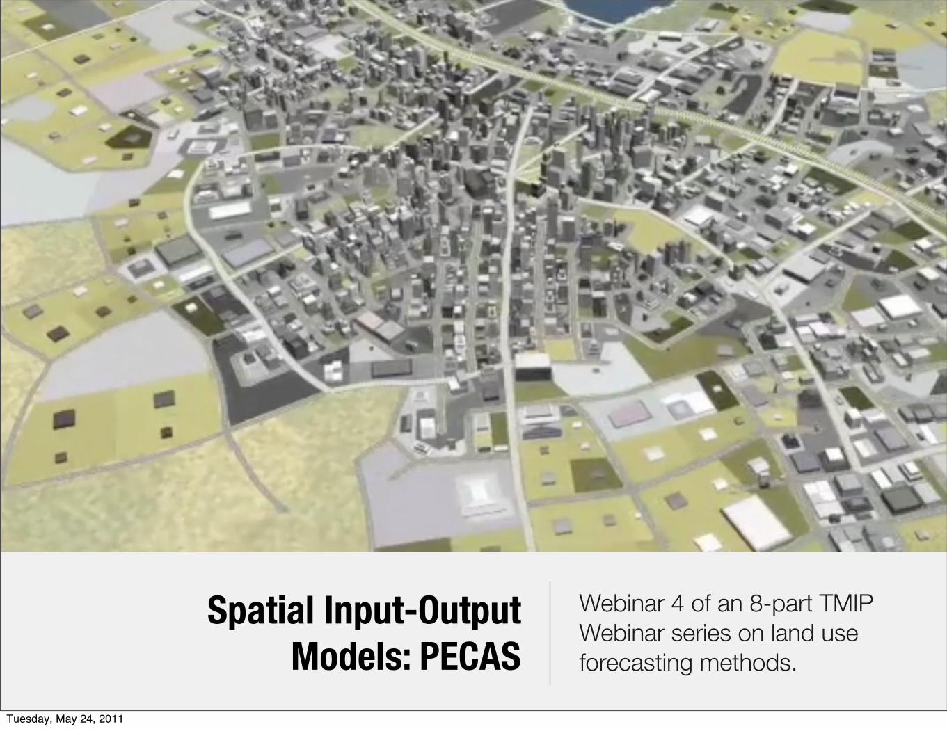
Spatial Input-Output Models: PECAS Webinar 4 of an 8-part TMIP Webinar series on land use forecasting methods. Tuesday, May 24, 2011
Transcript of Spatial Input-Output Models: PECAS · PDF fileSpatial Input-Output Models: PECAS Webinar 4 of...
Spatial Input-Output Models: PECAS
Webinar 4 of an 8-part TMIP Webinar series on land use forecasting methods.
Tuesday, May 24, 2011
Paul Waddell, 2011
1. PECAS Overviewa. Backgroundb. Theoretical Basisc. Software Implementationd. Data Inputs and Outputs
2. Anatomy of the Model3. Application in Practice4. Comparison and Assessment
Tuesday, May 24, 2011

Paul Waddell, 2011
PECAS Background
• PECAS (the Production, Exchange and Consumption Allocation System) is an urban and regional modeling tool to support transportation and economic planning
• Developed by Dr. Doug Hunt and Dr. John Abraham, University of Calgary
• Contains two principal models:
- Activity Allocation (AA): an aggregate, equilibrium Spatial Input-Output Model
- Spatial Development (SD): a disaggregate State-Transition model
• Developed initially as part of an Oregon Department of Transportation (ODOT) Statewide Modeling project as a replacement for a 1st generation statewide model using TRANUS
• Recently, CalTrans implemented a contract with UC Davis to support development of a California Statewide PECAS model, and to support MPOs within the state in the development of metropolitan level PECAS models
Tuesday, May 24, 2011

Paul Waddell, 2011
Application:Current Applications (from model developers)
• Oregon, USA State-wide
- part of larger modelling system with micro-simulation components
• Ohio, USA State-wide
- Model designed and used as basis for data collection
• Sacramento Area, USA
- Part of larger modelling system with micro-simulation components
• Calgary Region, Canada
- Design for new urban level modelling system
• Edmonton Region, Canada
- Design for new urban level modelling system
• Baltimore Metropolitan Area
- Design for new urban level modelling system
Tuesday, May 24, 2011

Paul Waddell, 2011
The State of the Practice: Survey of MPOs in 2010
5
Tuesday, May 24, 2011

Paul Waddell, 2011
Evolution of Land Use Model Frameworks
Aggregate Dynamic Discrete Choice
HUDS
Lowry:Gravity Model
Spatial InteractionDRAM/EMPAL
HLFM II+
Leontieff: Input-Output Model
Alonso/Mills/Muth:Urban EconomicBid-Rent Theory
Orcutt:Microsimulation
McFadden: Discrete-Choice
Models
1960
Aggregate EquilibriumDiscrete Choice
METROSIM; MUSSA
Spatial Input-OutputMEPLAN; TRANUS
Microsimulation Dynamic Discrete Choice
UrbanSim
Spatially DetailedRule-based Planning ToolsIndex; I-PLACE3S; WhatIf?
Geographic Information Systems
1970
1980
1990
2000
2010
PECAS
Tuesday, May 24, 2011
Paul Waddell, 2011
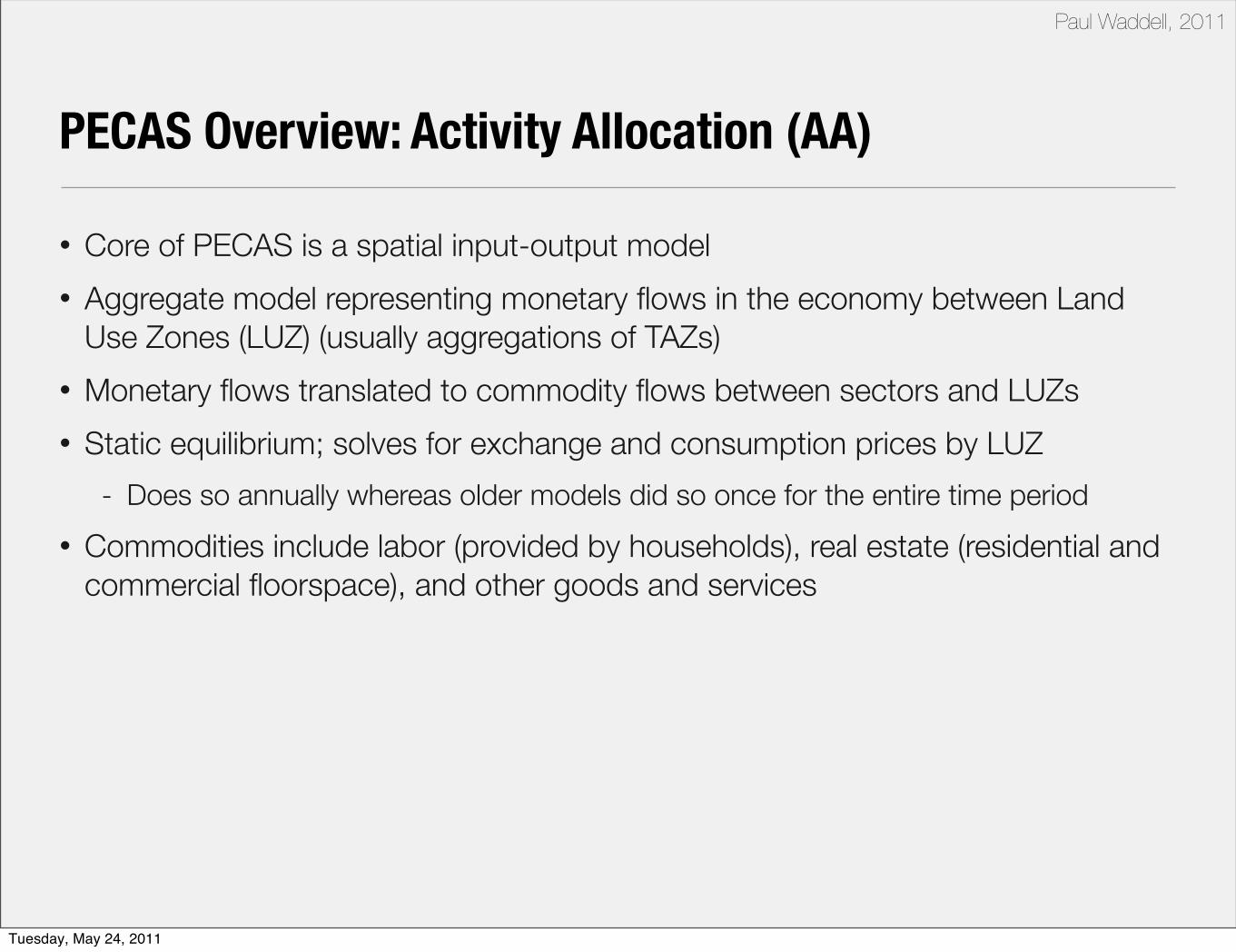
PECAS Overview: Activity Allocation (AA)
• Core of PECAS is a spatial input-output model
• Aggregate model representing monetary flows in the economy between Land Use Zones (LUZ) (usually aggregations of TAZs)
• Monetary flows translated to commodity flows between sectors and LUZs
• Static equilibrium; solves for exchange and consumption prices by LUZ
- Does so annually whereas older models did so once for the entire time period
• Commodities include labor (provided by households), real estate (residential and commercial floorspace), and other goods and services
Tuesday, May 24, 2011
Paul Waddell, 2011
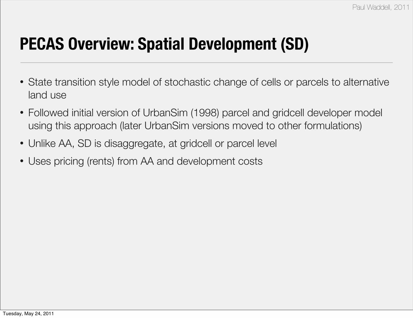
PECAS Overview: Spatial Development (SD)
• State transition style model of stochastic change of cells or parcels to alternative land use
• Followed initial version of UrbanSim (1998) parcel and gridcell developer model using this approach (later UrbanSim versions moved to other formulations)
• Unlike AA, SD is disaggregate, at gridcell or parcel level
• Uses pricing (rents) from AA and development costs
Tuesday, May 24, 2011

Paul Waddell, 2011
Theoretical Basis: Input-Output Models
• PECAS’s core (the AA) is a spatial input-output model
• This venerable approach represents an economy as a matrix
- cells contain values representing the amount of economic activity (production or consumption) for a particular combination of sectors
- equations represent the interlinkages between portions of the economy and allow changes in one area to be traced through to other areas
- tracking the activities and flows by geographic location makes the table spatial
• Now a brief review of this approach
Tuesday, May 24, 2011

Paul Waddell, 2011
In order to produce a total output of $20000, the retail sector consumes inputs for its production process. Assume the following inputs are purchased to produce the $20000 of retail output, based on the production process for retail:
Example I-O Expenditure Table for Retail
Retail
Basic
Retail
Services
$5000
$2000
$3000
Tuesday, May 24, 2011
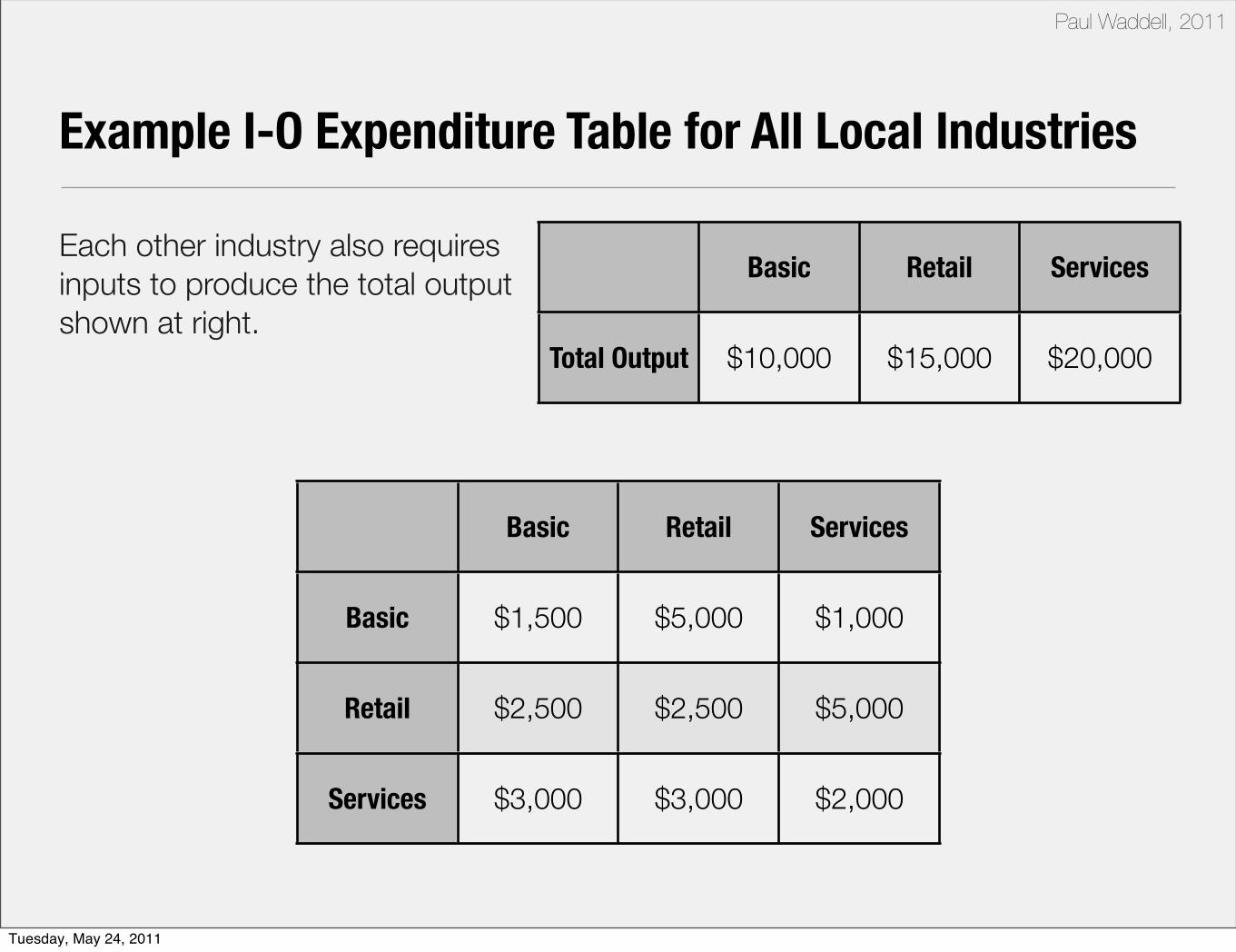
Each other industry also requires inputs to produce the total output shown at right.
Example I-O Expenditure Table for All Local Industries
Basic Retail Services
Basic
Retail
Services
$1,500 $5,000 $1,000
$2,500 $2,500 $5,000
$3,000 $3,000 $2,000
Basic Retail Services
Total Output $10,000 $15,000 $20,000
Paul Waddell, 2011
Tuesday, May 24, 2011

Paul Waddell, 2011
This table shows the standardized inputs per dollar of output for each industry, also known as technical coefficients.
Example I-O Direct Input Requirements Matrix
Basic Retail Services
Basic
Retail
Services
0.15 0.33 0.05
0.25 0.13 0.25
0.30 0.20 0.10
Tuesday, May 24, 2011
Paul Waddell, 2011
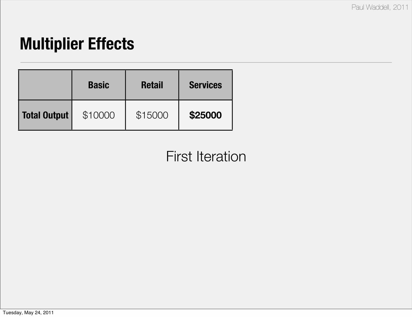
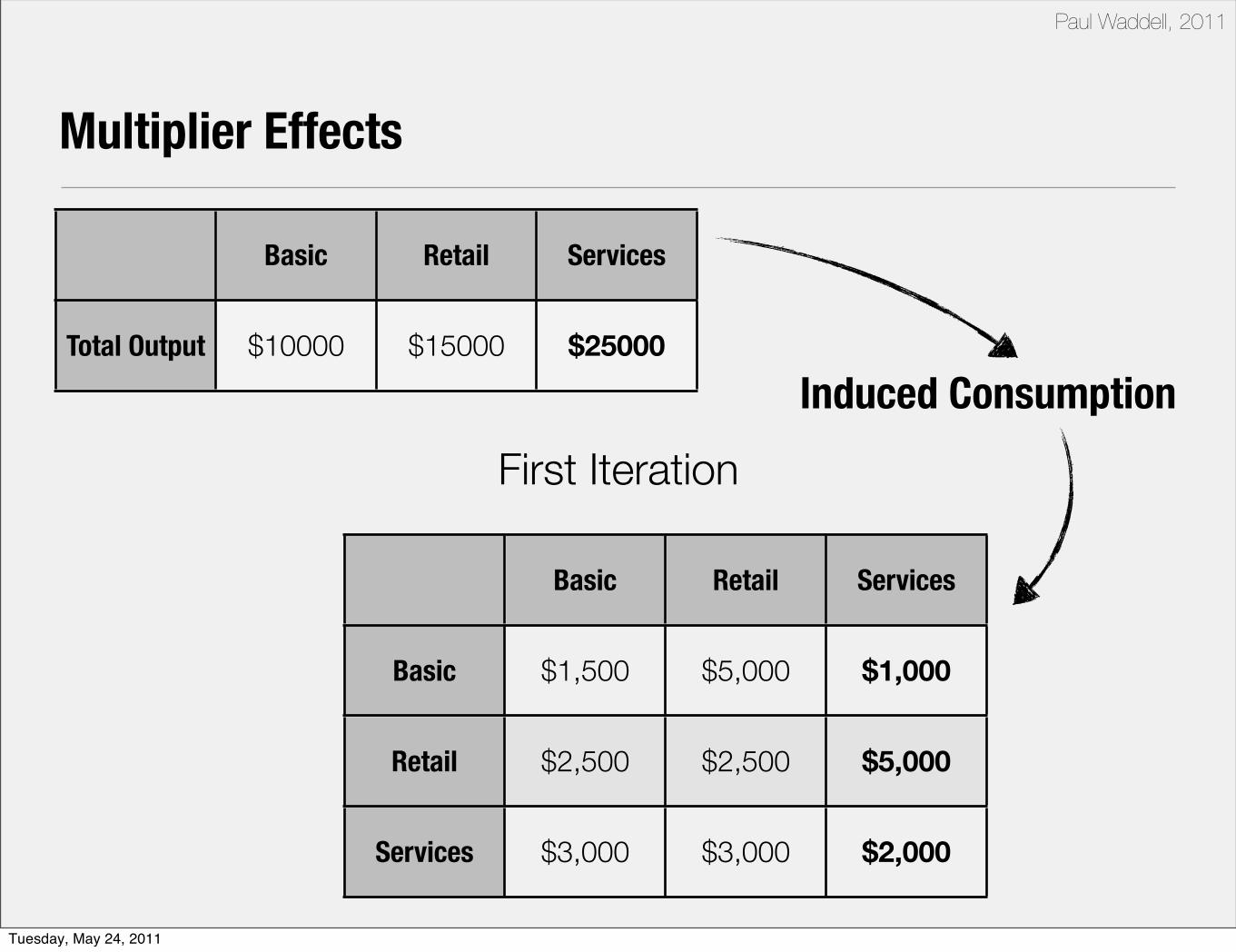
Multiplier Effects
Basic Retail Services
Total Output $10000 $15000 $25000
First Iteration
Tuesday, May 24, 2011

Paul Waddell, 2011
Multiplier Effects
Basic Retail Services
Total Output $10000 $15000 $25000
Induced Consumption
First Iteration
Tuesday, May 24, 2011
Paul Waddell, 2011
Multiplier Effects
Basic Retail Services
Total Output $10000 $15000 $25000
Induced Consumption
Basic Retail Services
Basic
Retail
Services
$1,500 $5,000 $1,000
$2,500 $2,500 $5,000
$3,000 $3,000 $2,000
First Iteration
Tuesday, May 24, 2011

Paul Waddell, 2011
Multiplier Effects
Basic Retail Services
Total Output $10000 $15000 $25000
Induced Consumption
Basic Retail Services
Basic
Retail
Services
$1,500 $5,000 $1,000
$2,500 $2,500 $5,000
$3,000 $3,000 $2,000
Basic Retail Services
Total Output $10,500 $16,250 $25,250
First Iteration
Tuesday, May 24, 2011

Paul Waddell, 2011
Basic Retail Services
Total Output $11,302 $17,344 $26,510
Multiplier Effects
Induced Consumption
Basic Retail Services
Basic
Retail
Services
$1,695 $5,781 $1,326
$2,826 $2,891 $6,628
$3,391 $3,469 $2,651
After Convergence
Tuesday, May 24, 2011

Paul Waddell, 2011
Economic Flows Can be Split by Region (Spatial I-O)
EconomicActivitiesEconomicActivitiesEconomicActivitiesEconomicActivities
Region ARegion ARegion A Region BRegion BRegion B Final Demand and Exports Total Demand
Basic Retail Services Basic Retail Services
Final Demand and Exports Total Demand
Region A
Basic
Region A RetailRegion A
Services
Region B
Basic
Region B RetailRegion B
Services
Final Paymentsand Imports
Final Paymentsand Imports
Total InputsTotal Inputs
Tuesday, May 24, 2011
Paul Waddell, 2011
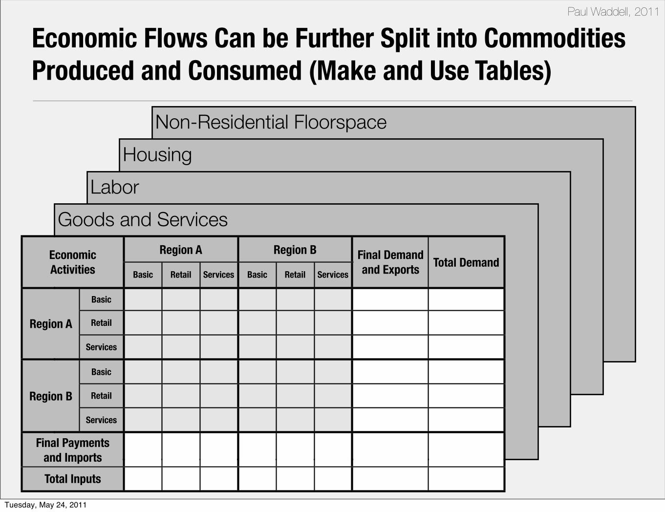
Economic Flows Can be Further Split into Commodities Produced and Consumed (Make and Use Tables)
EconomicActivitiesEconomicActivitiesEconomicActivitiesEconomicActivities
Region ARegion ARegion A Region BRegion BRegion B Final Demand and Exports Total Demand
Basic Retail Services Basic Retail Services
Final Demand and Exports Total Demand
Region A
Basic
Region A RetailRegion A
Services
Region B
Basic
Region B RetailRegion B
Services
Final Paymentsand Imports
Final Paymentsand Imports
Total InputsTotal Inputs
Tuesday, May 24, 2011
Paul Waddell, 2011
Non-Residential Floorspace
Economic Flows Can be Further Split into Commodities Produced and Consumed (Make and Use Tables)
Housing
Labor
Goods and Services
EconomicActivitiesEconomicActivitiesEconomicActivitiesEconomicActivities
Region ARegion ARegion A Region BRegion BRegion B Final Demand and Exports Total Demand
Basic Retail Services Basic Retail Services
Final Demand and Exports Total Demand
Region A
Basic
Region A RetailRegion A
Services
Region B
Basic
Region B RetailRegion B
Services
Final Paymentsand Imports
Final Paymentsand Imports
Total InputsTotal Inputs
Tuesday, May 24, 2011

Paul Waddell, 2011
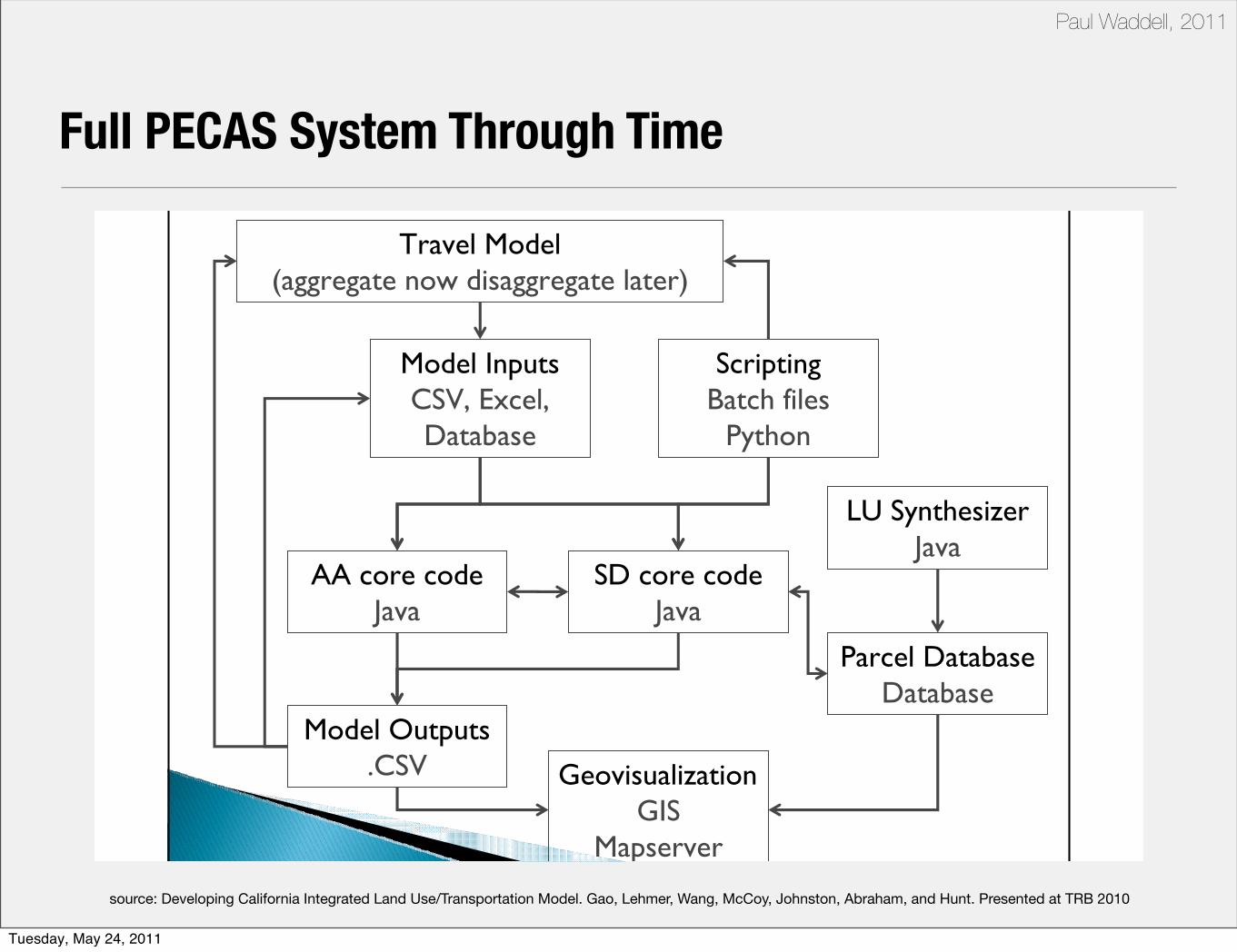
PECAS Software Architecture
• Base PECAS system consists of two major Java modules (the AA and the SD) and supporting infrastructure
• Model runs initiated using DOS shell or Python script
• Most data stored and passed between modules in CSV format
- Scenario inputs and parameters are set by creating CSV files
- Most model outputs are also in many CSV files
• Parcel information is stored in a database such as SQL Server or PostGIS
• Data preparation requires GIS and statistical software
• Loose integration with travel model through squeezed skims in CSV
• Runs on a multi-processor server
- Calibration can take days for a single run
- Multi-decade projections can take hours
Tuesday, May 24, 2011

Paul Waddell, 2011
Activity Allocation (AA) ModuleInputs and Data Sources (1)
• Aggregate economic flow: IMPLAN
- Demargined for wholesale and retail
• Synthetic households by TAZ
- Census PUMS
- Census SF 3 summary files
- Automated in Python
• Synthetic employment (by industry and occupation)
- CTPP
- InfoUSA
- Automated in Python
• Technology options
- Aggregate economic flow; Census PUMS; cluster analysis
Source: Shengyi Gao (et al)Tuesday, May 24, 2011
Paul Waddell, 2011
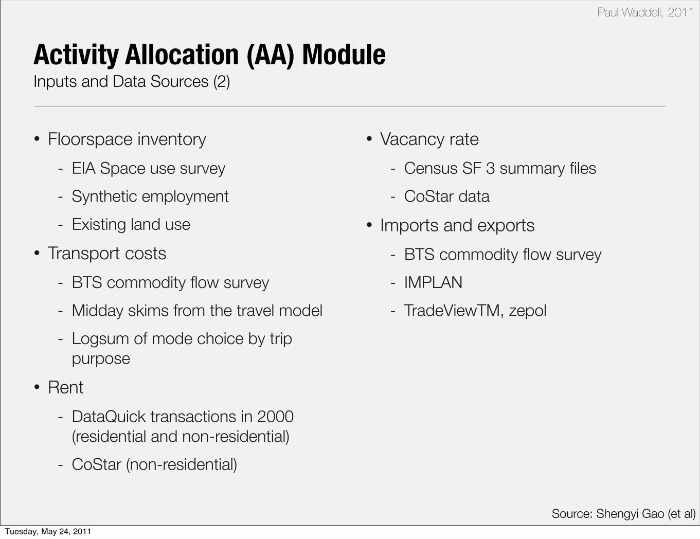
Activity Allocation (AA) ModuleInputs and Data Sources (2)
• Floorspace inventory
- EIA Space use survey
- Synthetic employment
- Existing land use
• Transport costs
- BTS commodity flow survey
- Midday skims from the travel model
- Logsum of mode choice by trip purpose
• Rent
- DataQuick transactions in 2000 (residential and non-residential)
- CoStar (non-residential)
• Vacancy rate
- Census SF 3 summary files
- CoStar data
• Imports and exports
- BTS commodity flow survey
- IMPLAN
- TradeViewTM, zepol
Source: Shengyi Gao (et al)Tuesday, May 24, 2011
Paul Waddell, 2011
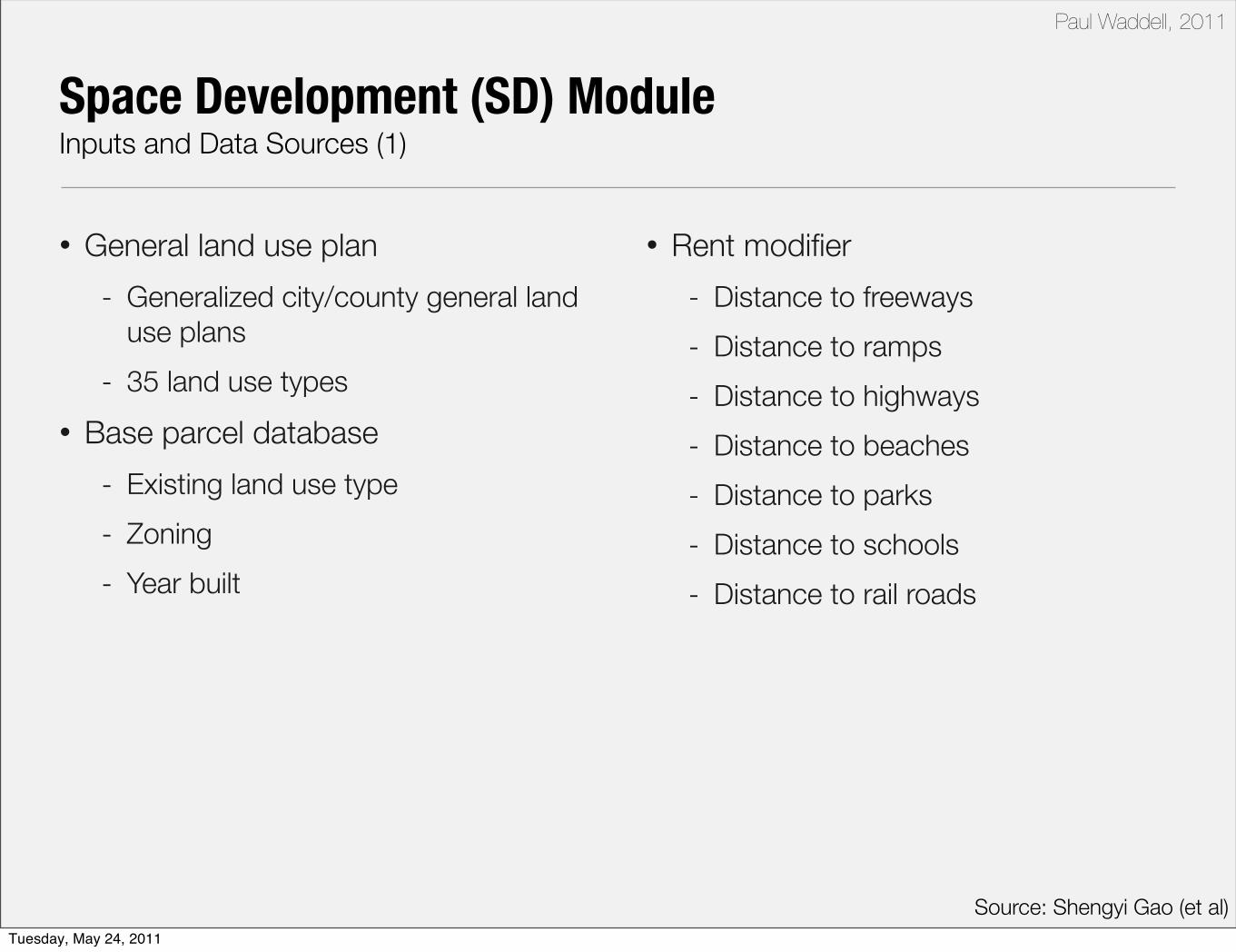
Space Development (SD) ModuleInputs and Data Sources (1)
• General land use plan
- Generalized city/county general land use plans
- 35 land use types
• Base parcel database
- Existing land use type
- Zoning
- Year built
• Rent modifier
- Distance to freeways
- Distance to ramps
- Distance to highways
- Distance to beaches
- Distance to parks
- Distance to schools
- Distance to rail roads
Source: Shengyi Gao (et al)Tuesday, May 24, 2011

Paul Waddell, 2011
Space Development (SD) ModuleInputs and Data Sources (2)
• Construction cost
- RSMeans data
• Maintenance cost
• Typical FAR
• Density rent discount
• Demolition costs
• Age discount
- Multiple sources
• Maximum/minimum intensity
- Zoning ordinance
• Development fees
- HCD database
Source: Shengyi Gao (et al)Tuesday, May 24, 2011
Paul Waddell, 2011
1. PECAS Overview
2. Anatomy of the Systema. Model Designb. Software Architecturec. Estimation, Calibration, and Validation
3. Application in Practice4. Comparison and Assessment
Tuesday, May 24, 2011
Paul Waddell, 2011
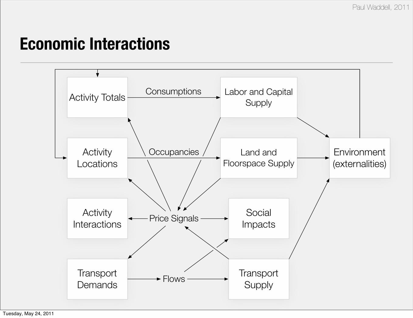
Activity Totals
Activity Locations
Activity Interactions
Transport Demands
Labor and Capital Supply
Land and Floorspace Supply
Social Impacts
Transport Supply
Price Signals
Flows
Environment (externalities)
Consumptions
Occupancies
Economic Interactions
Tuesday, May 24, 2011

Paul Waddell, 2011
PECAS Overview
Activity Totals
Activity Locations
Activity Interactions
Transport Demands
Labor and Capital Supply
Land and Floorspace Supply
Social Impacts
Transport Supply
Price Signals
Flows
Environment (externalities)
Consumptions
Occupancies
PECAS
Tuesday, May 24, 2011
Paul Waddell, 2011
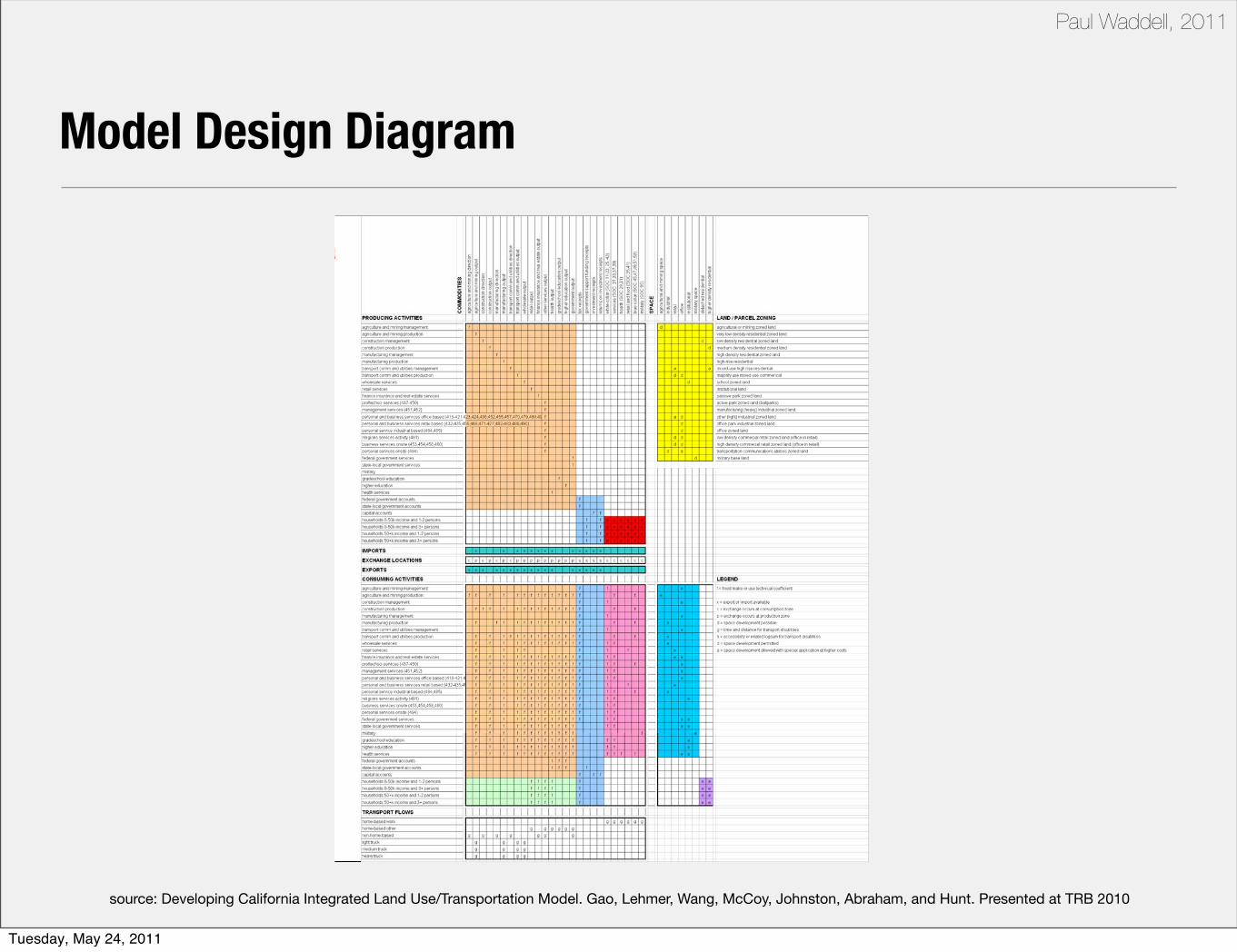
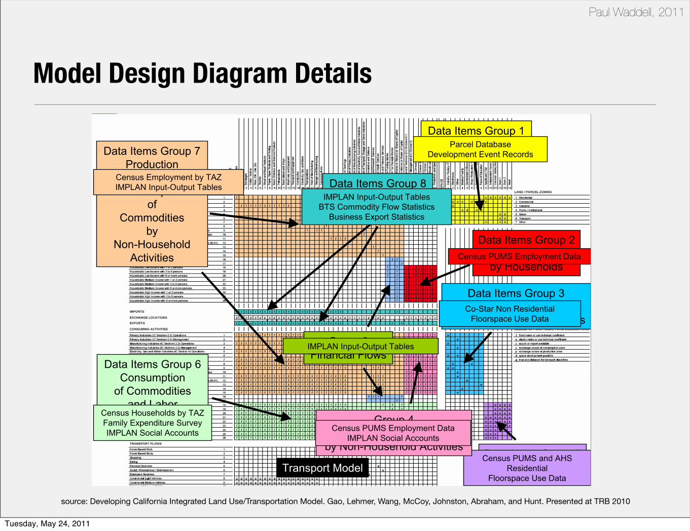
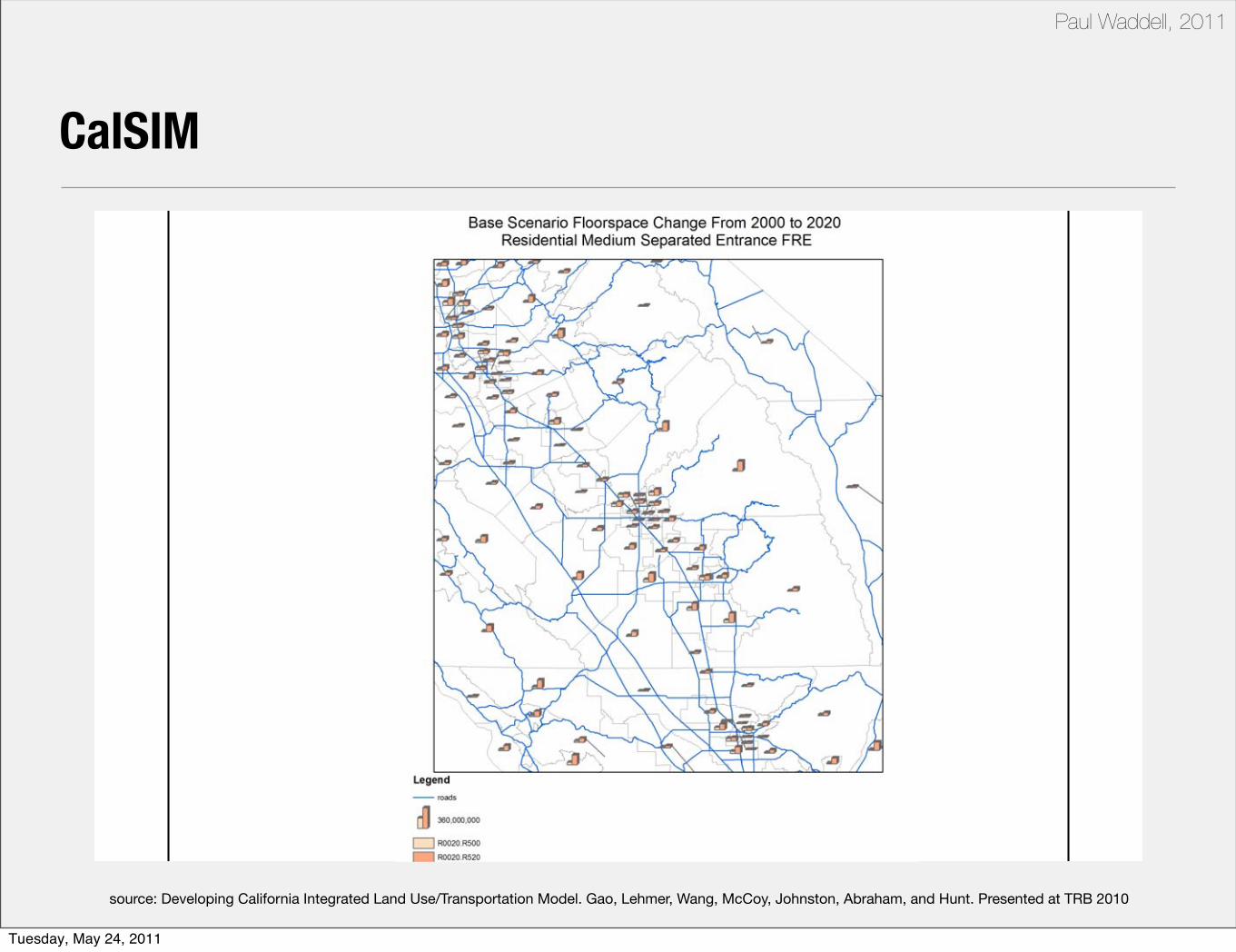
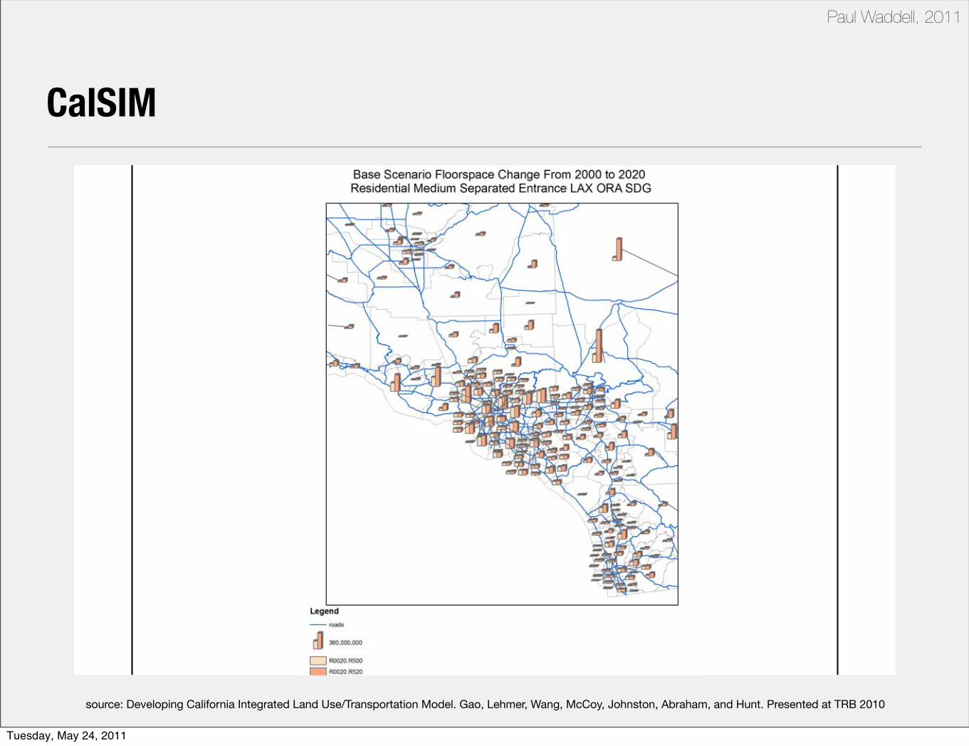
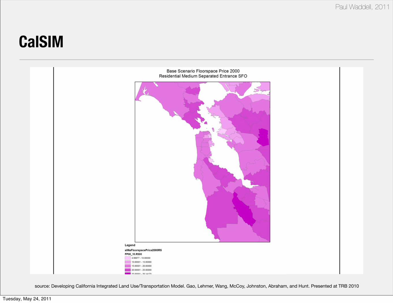
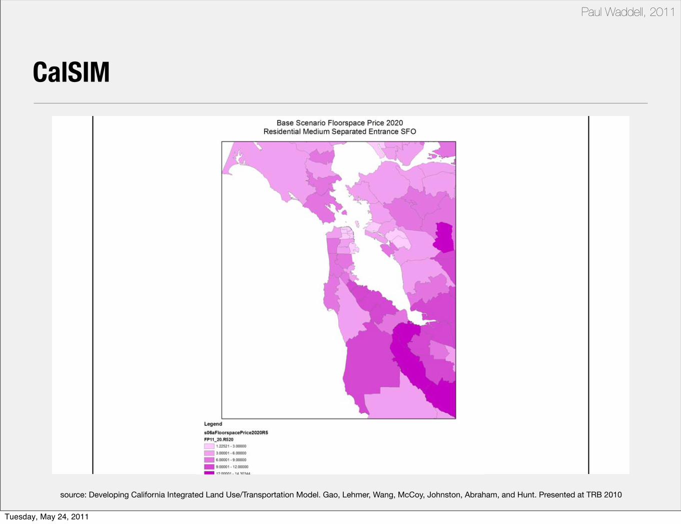
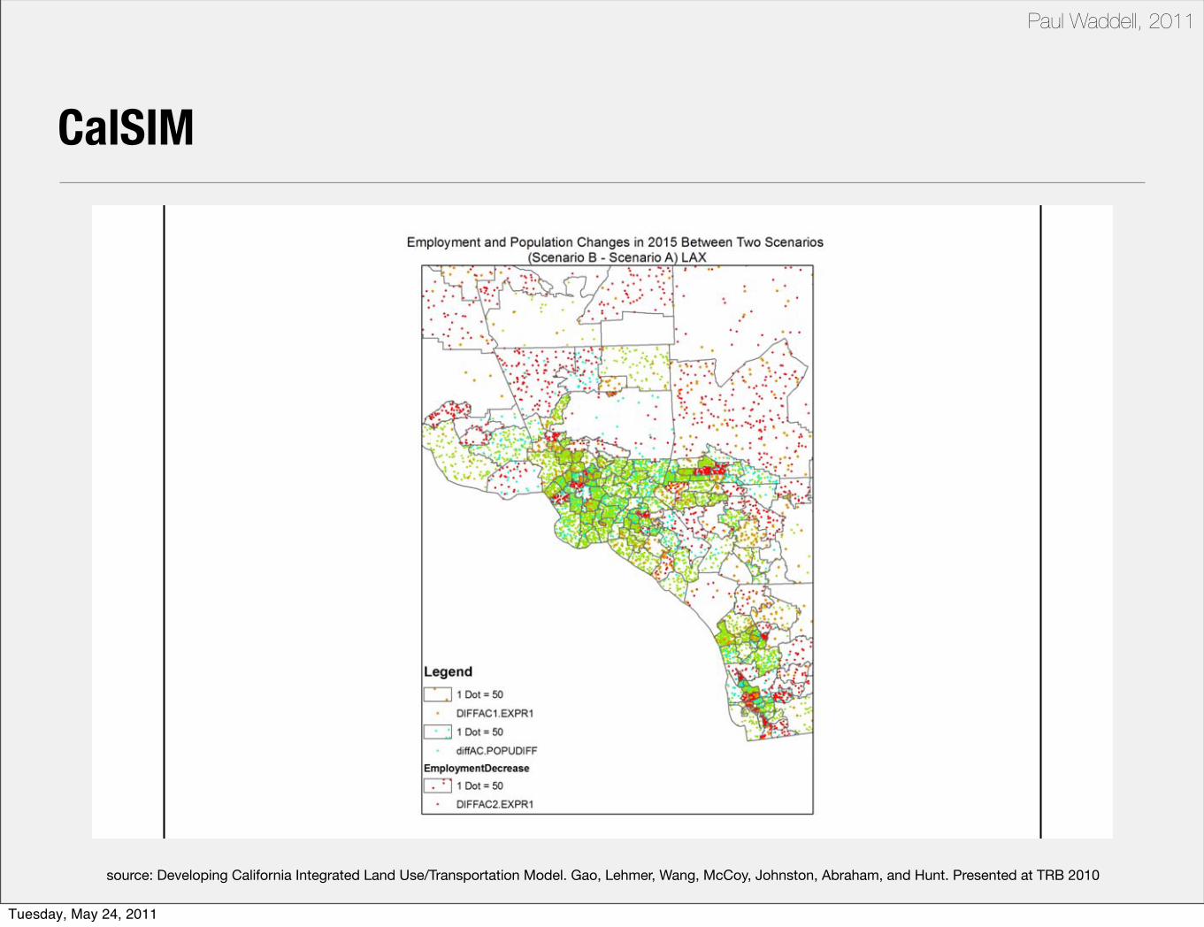
source: Developing California Integrated Land Use/Transportation Model. Gao, Lehmer, Wang, McCoy, Johnston, Abraham, and Hunt. Presented at TRB 2010
Atlanta
Model Design Diagram
Tuesday, May 24, 2011
Paul Waddell, 2011
source: Developing California Integrated Land Use/Transportation Model. Gao, Lehmer, Wang, McCoy, Johnston, Abraham, and Hunt. Presented at TRB 2010
Data Items Group 1Space Development
Data Items Group 2Production of Labor
by Households
Data Items Group 3Use of Space
by Non-Household Activities
Data Items Group 5Use of Space
by Households
Data Items Group 6Consumption
of Commoditiesand Labor
by Households
Data Items Group 7Production
andConsumption
ofCommodities
byNon-Household
Activities
Data Items Group 8Imports and Exports
of Commodities
Parcel DatabaseDevelopment Event Records
Census Households by TAZFamily Expenditure SurveyIMPLAN Social Accounts
Census Employment by TAZIMPLAN Input-Output Tables
Census PUMS Employment Data
IMPLAN Input-Output TablesBTS Commodity Flow Statistics
Business Export Statistics
Co-Star Non Residential Floorspace Use Data
Census PUMS and AHSResidential
Floorspace Use DataTransport ModelTransport Model
Group 4Use of Labor
by Non-Household Activities
Census PUMS Employment DataIMPLAN Social Accounts
Group 9Financial Flows
IMPLAN Input-Output Tables
Model Design Diagram Details
Tuesday, May 24, 2011

Paul Waddell, 2011
Activity Allocation (AA) Module
• Aggregate spatial input-output model
• Represents interaction of activities through commodity flows
- Food shipping to a processing plant to store
- Person driving to work
• Travel model provides the yearly description of disutility of movement between locations (congestion) that underly activity interaction
- e.g Congestion might move two interdependent industries closer together
- e.g. A new highway might drive development of new subdivisions
• Connection with SD
- Activities occupy floorspace build by the SD
- Spatial choices of activities drive prices that motivate SD developer
Tuesday, May 24, 2011
Paul Waddell, 2011
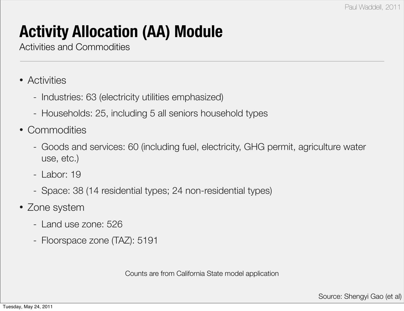
Activity Allocation (AA) ModuleActivities and Commodities
• Activities
- Industries: 63 (electricity utilities emphasized)
- Households: 25, including 5 all seniors household types
• Commodities
- Goods and services: 60 (including fuel, electricity, GHG permit, agriculture water use, etc.)
- Labor: 19
- Space: 38 (14 residential types; 24 non-residential types)
• Zone system
- Land use zone: 526
- Floorspace zone (TAZ): 5191
Source: Shengyi Gao (et al)
Counts are from California State model application
Tuesday, May 24, 2011

Paul Waddell, 2011
Activity Allocation (AA) ModuleDecision Tree
Location Choices
Production/Consumption Choices
Exchange Location Choices
Tuesday, May 24, 2011
Paul Waddell, 2011
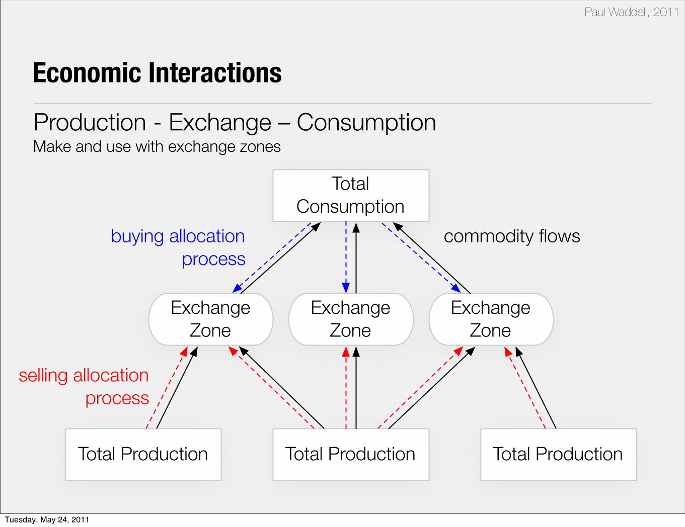
Economic Interactions
Production - Exchange – ConsumptionMake and use with exchange zones
Total Consumption
Total Production
Exchange Zone
Total Production
Exchange Zone
Total Production
Exchange Zone
commodity flowsbuying allocationprocess
selling allocationprocess
Tuesday, May 24, 2011

Paul Waddell, 2011
Economic Interactions
Production - Exchange – Consumption
technology selection
1:
2:
3:buying
allocations
selling allocations
production allocation
allocating production activity to zones
allocating consumption to
commodities
allocating production to commodities
allocating produced commodities to selling locations
allocating consumed commodities to buying locations
3-level nested logit modelTuesday, May 24, 2011

Paul Waddell, 2011
Activity Allocation (AA) ModuleJoint Discrete Utility
Source: Atlanta Regional Commission
Additional utility associated with location l for activity a
Additional utility associated with production option p
Stochastic error terms
Utility of exchanging and shipping one unit of
commodity between l and e
Quantity of commodity produced or consumed
under production option p
Tuesday, May 24, 2011

Paul Waddell, 2011
Space Development (SD) Module
• Disaggregate process at the parcel level
- Grid cells or parcels
• Represent developers’ actions
• Connection with AA
- From AA: current year space price at LUZ level
- To AA: quantity of the spaces for next year AA
• Space is a commodity consumed by the activities in the AA model
- Unlike other commodities, space cannot be transported
- Different activities consume different types of space• e.g. in Atlanta there are 8 PECAS space types (A/D/S/M/O/R/L/H)
• Rents are space prices
• Zoning rules limit the type of space the can be developed on a parcel
Source: Atlanta Regional CommissionTuesday, May 24, 2011

Paul Waddell, 2011
Space Development (SD) ModuleDevelopment Events
• Year-by-year step
• Possible development events
- E0: no change
- En: new space type and quantity
- Er: alter or renovate
- Ed: derelict
• Two step process for each parcel
- Selection of development events and update space type
- Update space amount
• Data needs
- Permits
- Parcel level data
- Rents
Source: Atlanta Regional CommissionTuesday, May 24, 2011

Paul Waddell, 2011
• Space prices are rents for the use of space
• Per unit of space per unit of time
• Rent equation:
- Space price at LUZ level in AA (done by AA & SD integration)
- Local-level effects due to:• Density of development around the parcel
• Age of the structure
• Local Effects: distance from (or proximity to) local-level influences
• Expressway
• Interstate exit
• Major road
• School
• Marta
• Green space
Space Development (SD) ModuleRents
Source: Atlanta Regional CommissionTuesday, May 24, 2011

Paul Waddell, 2011
Space Development (SD) ModuleSimulation of Transitions
more the sam
e
no change
mid density residential
comm
ercial
industrial
derelict
zoning dictates set of alternatives
Parcel-by-parcel microsimulation
Source: Atlanta Regional Commission
quantity
Tuesday, May 24, 2011
Paul Waddell, 2011
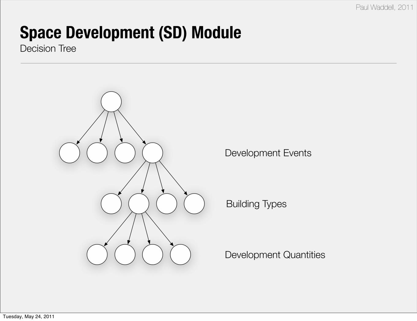
Development Events
Building Types
Development Quantities
Space Development (SD) ModuleDecision Tree
Tuesday, May 24, 2011
Paul Waddell, 2011
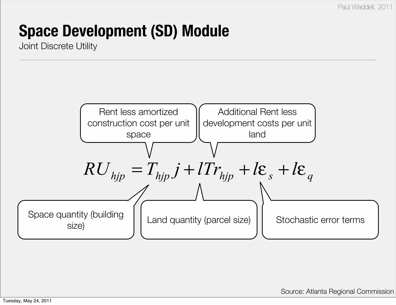
Space Development (SD) ModuleJoint Discrete Utility
Source: Atlanta Regional Commission
Rent less amortized construction cost per unit
space
Additional Rent less development costs per unit
land
Space quantity (building size)
Land quantity (parcel size) Stochastic error terms
Tuesday, May 24, 2011

Paul Waddell, 2011
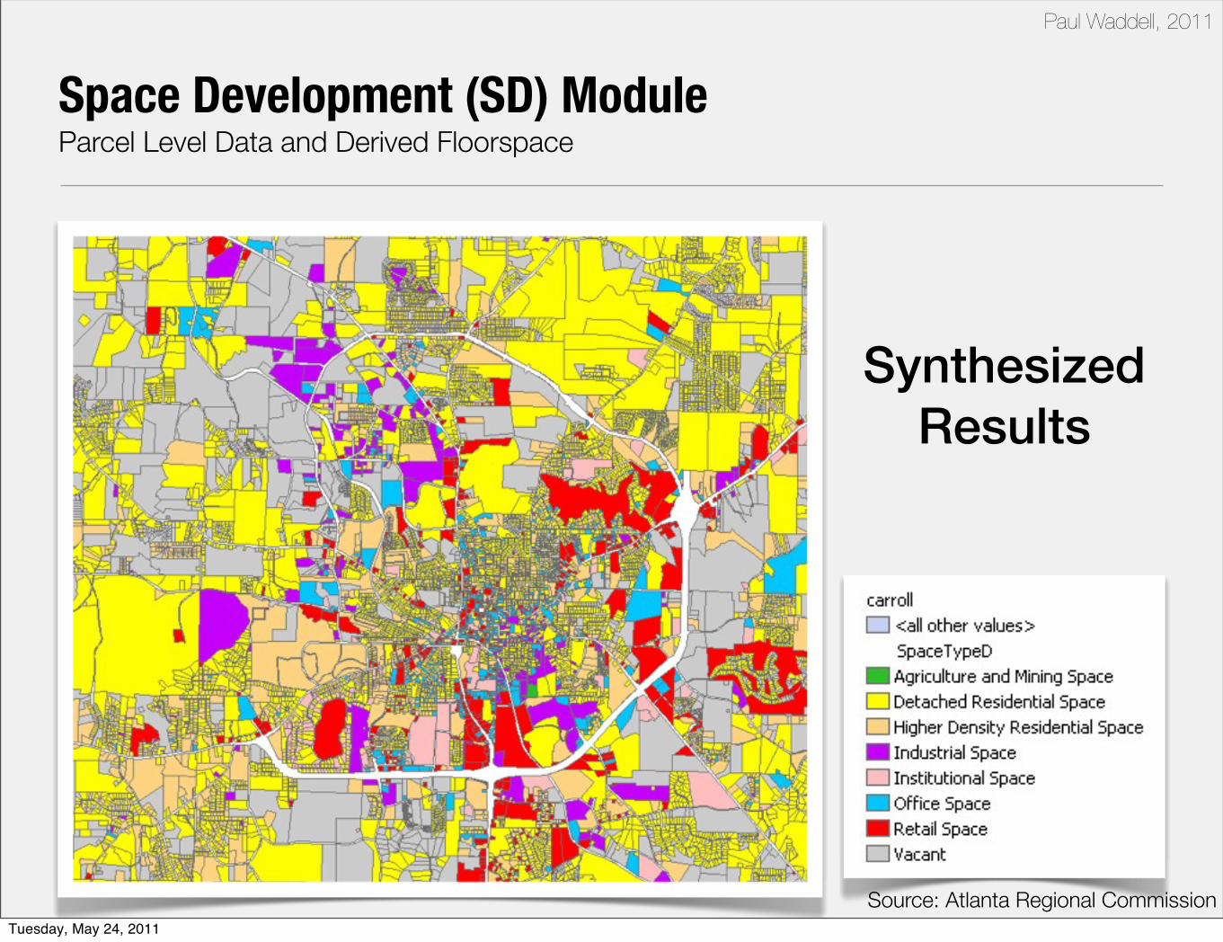
Space Development (SD) ModuleParcel Level Data and Derived Floorspace
• For each parcel:
- Area of the parcel
- Existing space type
- Existing space quantity (building floorspace)
- Structure year
- Zoning rules (allowable uses and density range)
- Cost and fees (associated with development of each permitted space type and quantity)
• Challenges (20 Counties: every dataset is different)
- Parcel features and ID
- Parcel attributes (building floorspace, space type…)
- Geocoded points for Clayton…
- Combine parcel with tax assessors’ data
- Updates
• 20-county parcels are cleaned and loaded
- About 2 million parcels are cleaned
• Benefit other planning projects
Source: Atlanta Regional CommissionTuesday, May 24, 2011
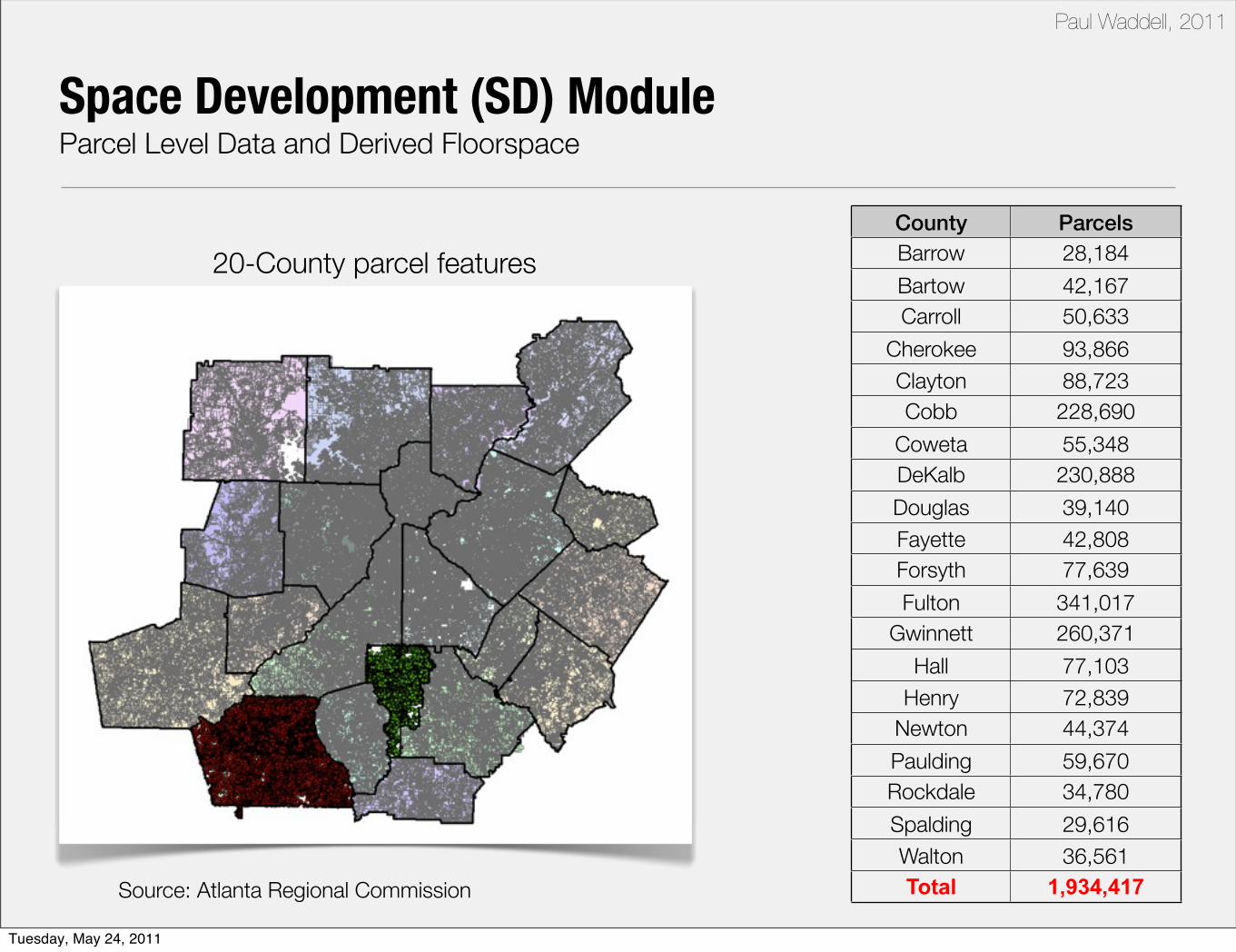
Paul Waddell, 2011
Space Development (SD) ModuleParcel Level Data and Derived Floorspace
County ParcelsBarrow 28,184
Bartow 42,167Carroll 50,633
Cherokee 93,866Clayton 88,723Cobb 228,690
Coweta 55,348DeKalb 230,888
Douglas 39,140Fayette 42,808Forsyth 77,639
Fulton 341,017Gwinnett 260,371
Hall 77,103Henry 72,839
Newton 44,374
Paulding 59,670Rockdale 34,780
Spalding 29,616Walton 36,561Total 1,934,417
20-County parcel features
Source: Atlanta Regional Commission
Tuesday, May 24, 2011
Paul Waddell, 2011
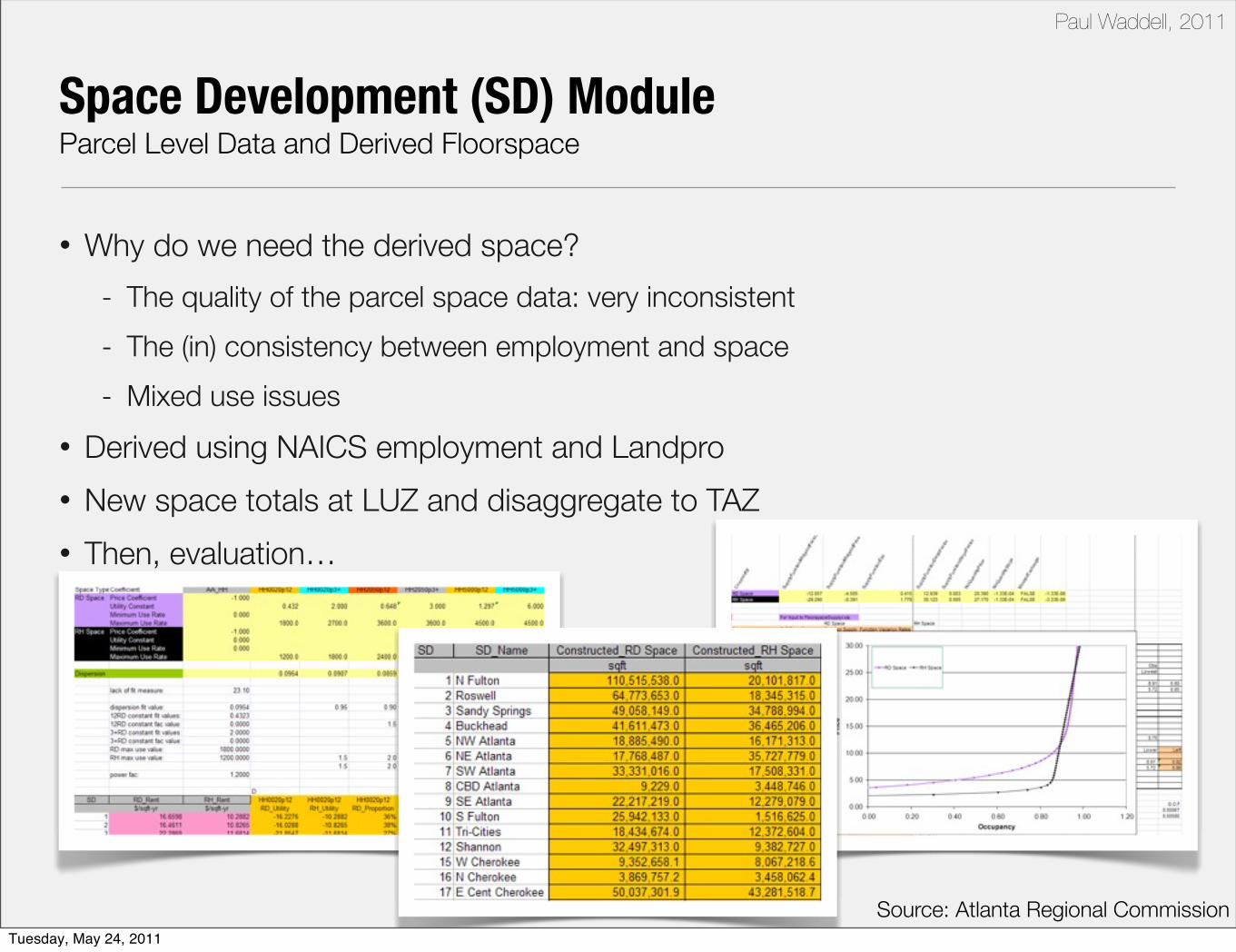
• Why do we need the derived space?
- The quality of the parcel space data: very inconsistent
- The (in) consistency between employment and space
- Mixed use issues
• Derived using NAICS employment and Landpro
• New space totals at LUZ and disaggregate to TAZ
• Then, evaluation…
Space Development (SD) ModuleParcel Level Data and Derived Floorspace
Source: Atlanta Regional CommissionTuesday, May 24, 2011

Paul Waddell, 2011
• FloorSpace Synthesizer Tool
• Based on existing space type, quantity and zoning…
• Calibration
Space Development (SD) ModuleParcel Level Data and Derived Floorspace
Source: Atlanta Regional CommissionTuesday, May 24, 2011
Paul Waddell, 2011
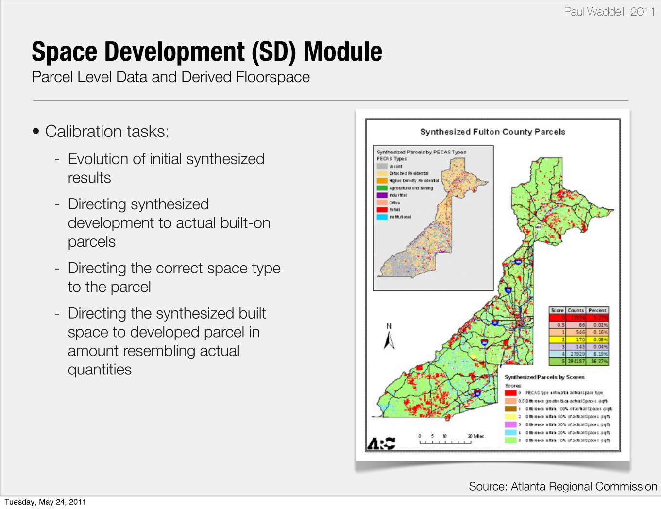
Space Development (SD) ModuleParcel Level Data and Derived Floorspace
• Calibration tasks:
- Evolution of initial synthesized results
- Directing synthesized development to actual built-on parcels
- Directing the correct space type to the parcel
- Directing the synthesized built space to developed parcel in amount resembling actual quantities
Source: Atlanta Regional CommissionTuesday, May 24, 2011
Paul Waddell, 2011
Space Development (SD) ModuleParcel Level Data and Derived Floorspace
Synthesized Results
Source: Atlanta Regional CommissionTuesday, May 24, 2011
Paul Waddell, 2011
source: Developing California Integrated Land Use/Transportation Model. Gao, Lehmer, Wang, McCoy, Johnston, Abraham, and Hunt. Presented at TRB 2010
AA core codeJava
SD core codeJava
Parcel DatabaseDatabase
GeovisualizationGIS
Mapserver
ScriptingBatch files
Python
Model InputsCSV, Excel,Database
Model Outputs.CSV
LU SynthesizerJava
Travel Model(aggregate now disaggregate later)
Full PECAS System Through Time
Tuesday, May 24, 2011
Paul Waddell, 2011
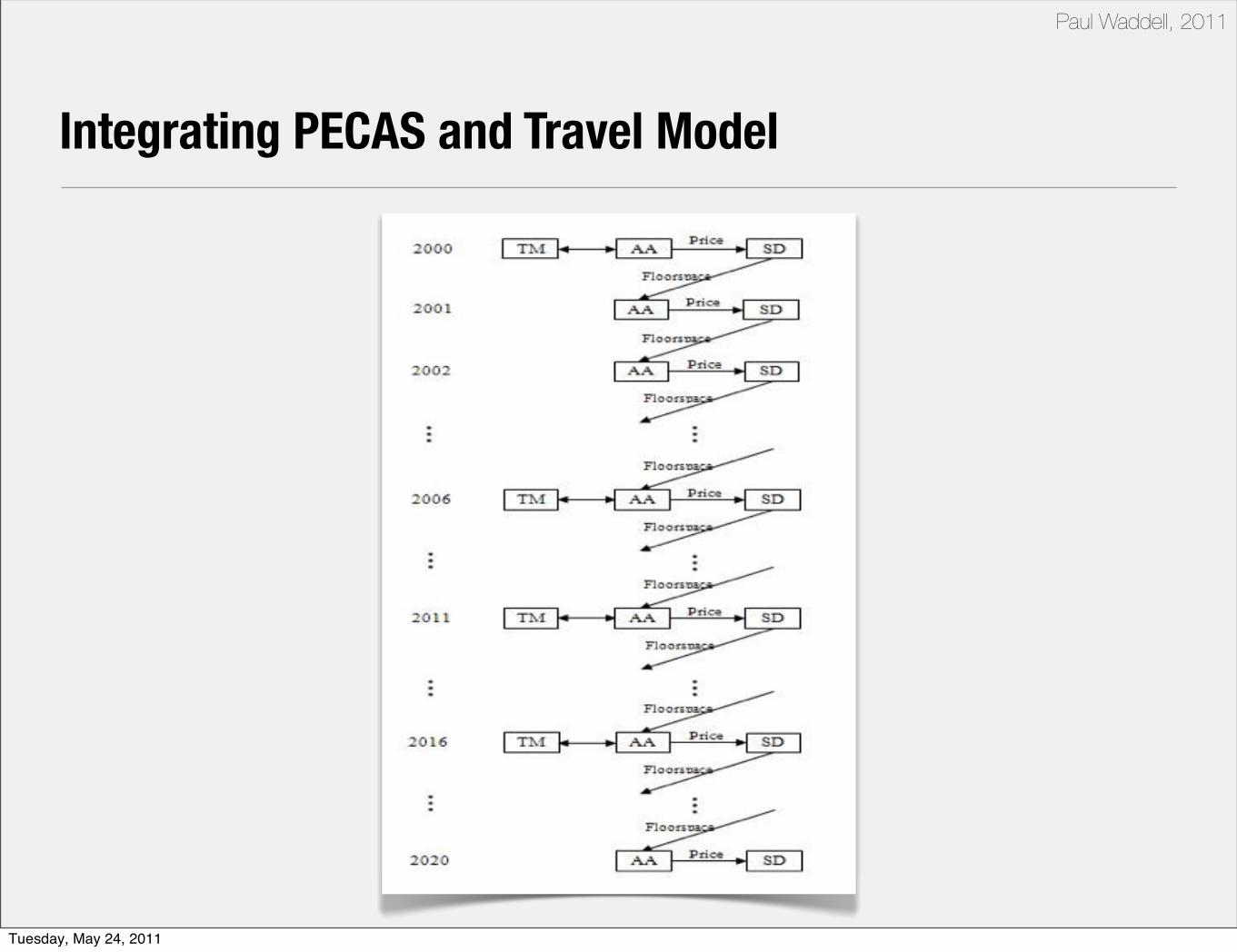
Integrating PECAS and Travel Model
Tuesday, May 24, 2011

Paul Waddell, 2011
PECAS 3-Stage Calibration Approach
• Stage 1 - the S1 parameters
- Consider each module separately
- Based on specific, separate dataset
- Often ‘disaggregate data’
- Often statistical estimation
- Fixed for remainder of calibration
• Stage 2 - the S2 parameters
- Consider each module separately
- Based on module hitting targets
- Often ‘aggregate data’
- Some also S3 parameters
- Specialized software developed
• Stage 3 - the S3 parameters
- Consider all modules linked together
- Based on module hitting targets
- ‘Aggregate data’
- Certain S2 parameters also S3 parameters, process updates these in response to total model behaviour
- Specialized software developed
Tuesday, May 24, 2011

Paul Waddell, 2011
Calibration Targets
AA Calibration Targets
• Buying and selling choice
- Distance to buy or sell
- CFS survey
• Technology choice
- Synthetic population
- PUMS
- Cluster analysis
• Location choice
- Synthetic population
- Synthetic employment
SD Calibration Targets
• Transition constant
- Building permit
- Parcel data at two time points
• Dispersion parameter
- Existing land use
Source: Shengyi Gao (et al)Tuesday, May 24, 2011

Paul Waddell, 2011
1. PECAS overview2. Anatomy of the System
3. Application in Practice4. Comparison and Assessment
Tuesday, May 24, 2011
Paul Waddell, 2011
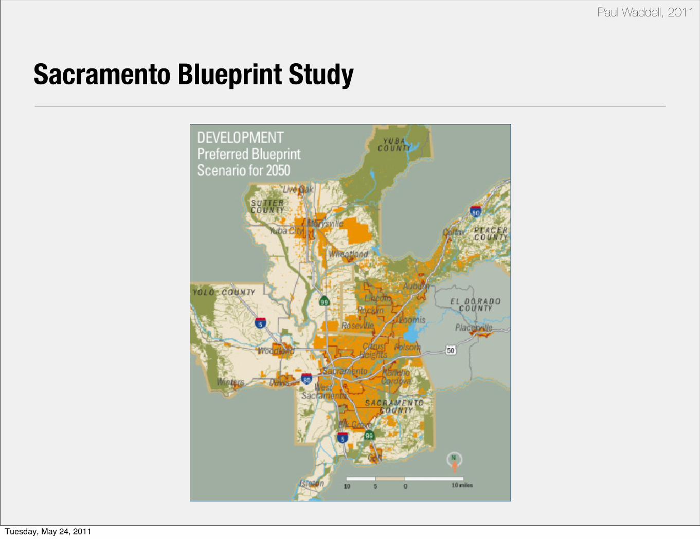
Sacramento Blueprint Study
Tuesday, May 24, 2011

Paul Waddell, 2011
Sacramento Blueprint Study
Tuesday, May 24, 2011
Paul Waddell, 2011
Sacramento Blueprint Study
Tuesday, May 24, 2011
Paul Waddell, 2011
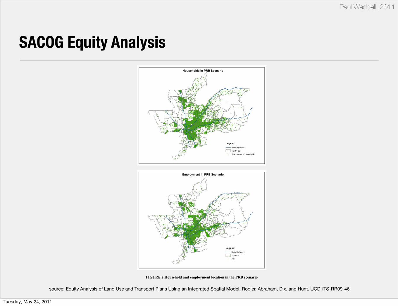
source: Equity Analysis of Land Use and Transport Plans Using an Integrated Spatial Model. Rodier, Abraham, Dix, and Hunt. UCD-ITS-RR09-46
6
FIGURE 2 Household and employment location in the PRB scenario
SACOG Equity Analysis
Tuesday, May 24, 2011
Paul Waddell, 2011
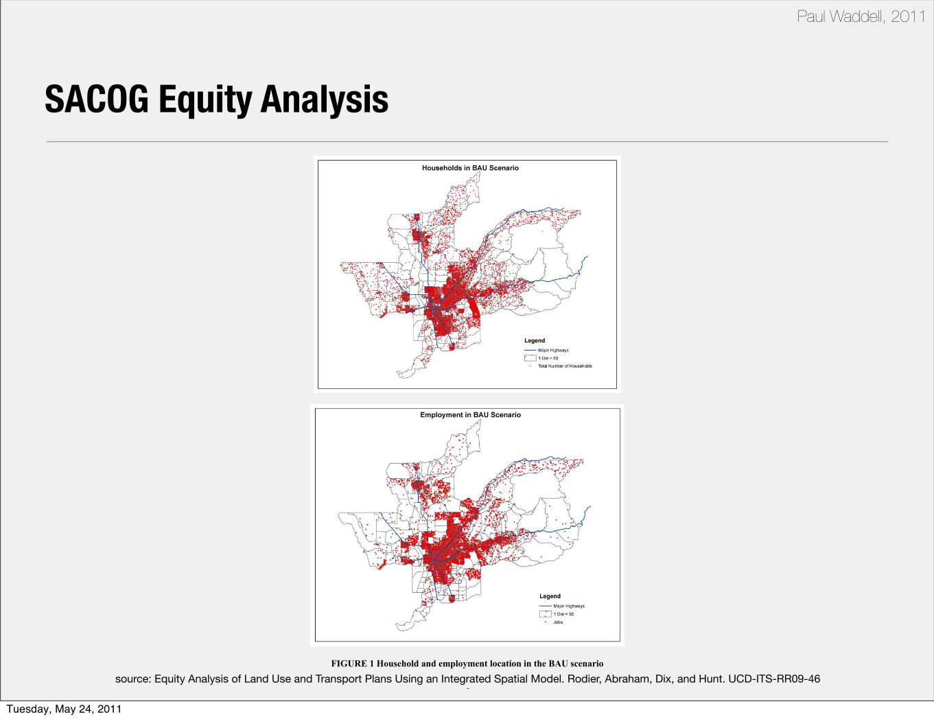
source: Equity Analysis of Land Use and Transport Plans Using an Integrated Spatial Model. Rodier, Abraham, Dix, and Hunt. UCD-ITS-RR09-46
5
FIGURE 1 Household and employment location in the BAU scenario
SACOG Equity Analysis
Tuesday, May 24, 2011

Paul Waddell, 2011
source: Equity Analysis of Land Use and Transport Plans Using an Integrated Spatial Model. Rodier, Abraham, Dix, and Hunt. UCD-ITS-RR09-46
7
FIGURE 3 Percent Change in Dwelling Units by Type Between the BAU and the PRB
SFD=single family dwelling units; MFD=multi family dwelling units
SACOG Equity Analysis
Tuesday, May 24, 2011
Paul Waddell, 2011
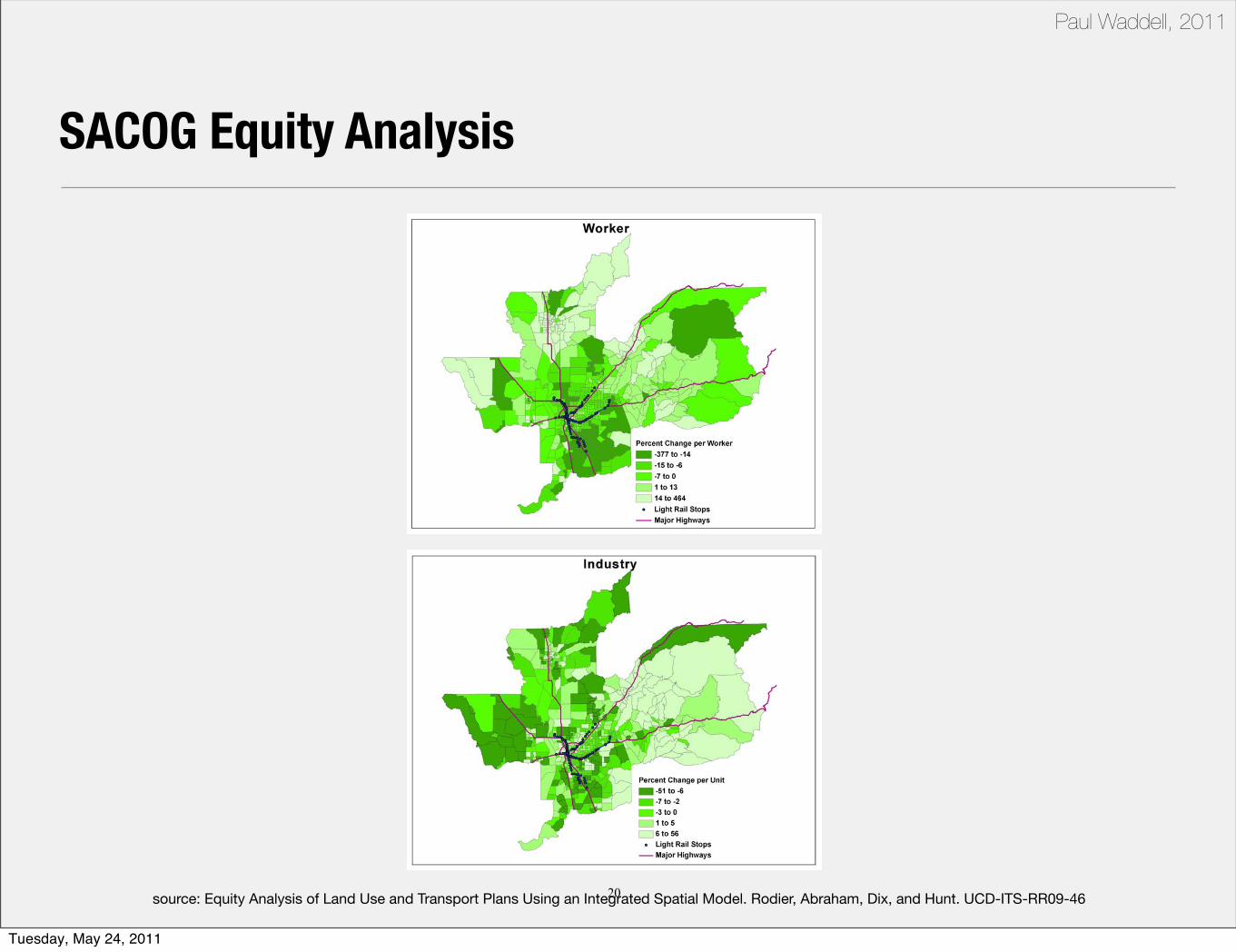
source: Equity Analysis of Land Use and Transport Plans Using an Integrated Spatial Model. Rodier, Abraham, Dix, and Hunt. UCD-ITS-RR09-46
20
SACOG Equity Analysis
Tuesday, May 24, 2011
Paul Waddell, 2011
source: Equity Analysis of Land Use and Transport Plans Using an Integrated Spatial Model. Rodier, Abraham, Dix, and Hunt. UCD-ITS-RR09-46
21
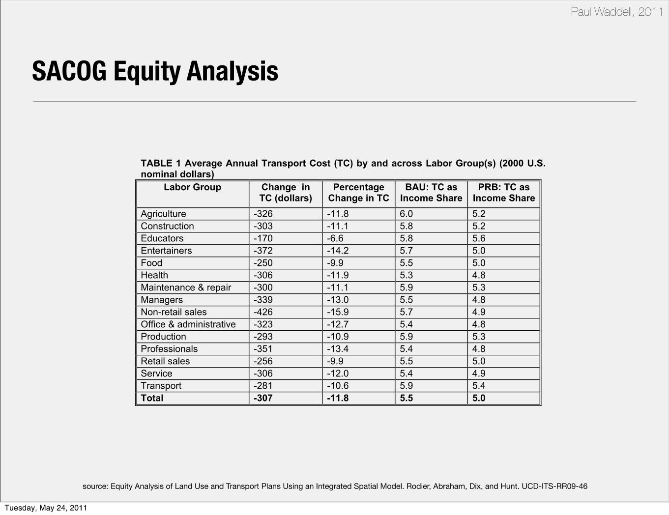
FIGURE 7 Percentage change in annual worker and industry transport cost from the BAU to the PRB scenario
TABLE 1 Average Annual Transport Cost (TC) by and across Labor Group(s) (2000 U.S. nominal dollars)
Labor Group Change in TC (dollars)
Percentage Change in TC
BAU: TC as Income Share
PRB: TC as Income Share
Agriculture -326 -11.8 6.0 5.2 Construction -303 -11.1 5.8 5.2 Educators -170 -6.6 5.8 5.6 Entertainers -372 -14.2 5.7 5.0 Food -250 -9.9 5.5 5.0 Health -306 -11.9 5.3 4.8 Maintenance & repair -300 -11.1 5.9 5.3 Managers -339 -13.0 5.5 4.8 Non-retail sales -426 -15.9 5.7 4.9 Office & administrative -323 -12.7 5.4 4.8 Production -293 -10.9 5.9 5.3 Professionals -351 -13.4 5.4 4.8 Retail sales -256 -9.9 5.5 5.0 Service -306 -12.0 5.4 4.9 Transport -281 -10.6 5.9 5.4 Total -307 -11.8 5.5 5.0
SACOG Equity Analysis
Tuesday, May 24, 2011
Paul Waddell, 2011
source: Equity Analysis of Land Use and Transport Plans Using an Integrated Spatial Model. Rodier, Abraham, Dix, and Hunt. UCD-ITS-RR09-46
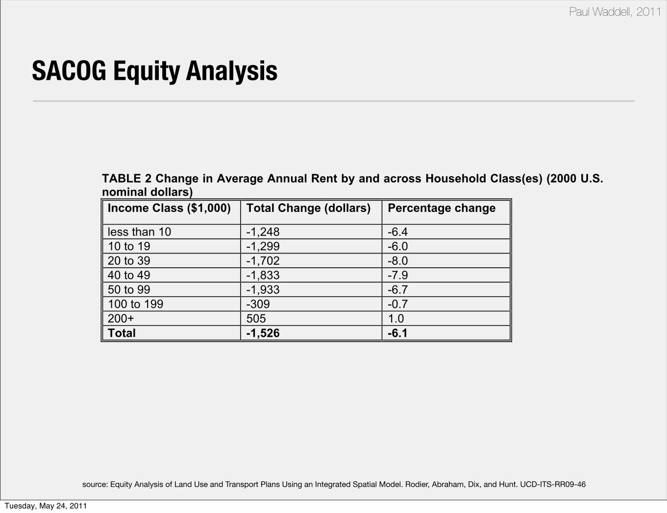
22
Average annual rents also decline in the region in the PRB scenario relative to the BAU (see Table 2). As described above, the total distribution of housing units by type in the PRB scenario represents a 10.9% increase in the number of multi-family units and 6.3% reduction in luxury single family dwelling units. Because of the greater supply of multi-family housing units, which are typically less expensive, average annual rents, for all but the highest income classes, are reduced in the PRB scenario. On average, rents are reduced by $1,526, which is a 6.1% reduction. The three lowest household income classes experience reductions in annual rent ranging from $1,248 to $1,702 (percentage reductions from 6.4% to 8%). Note that according to federal government standards, the lowest household income class (less than $10,000 a year) is considered to be extremely low income (or approximately 30% of the Sacramento area median income or AMI), $10,000 to $19,000 is very low income (or approximately 50% of AMI), and $20,000 to $39,000 is low income (or approximately 80% of AMI). The middle income classes ($20,000 to $99,000) see the greatest total reduction in rent. The highest income class ($200,000 and above) experiences an increase in rent ($505), which is a 1.0% increase. The second highest income class experiences the lowest reduction in rent ($309 and 0.7%).
In sum, it appears that the preference among the highest income households for larger homes and lots, the relatively diminished supply, and higher transport costs in the outer suburban areas where such homes are typically located have driven up average rents for the highest income class and mitigated declines relative to the regional mean. It also appears that the low and middle income household categories have benefited from the significantly increased supply of multi-family housing and lower transport costs in the areas in which they are located (i.e., the inner suburbs and central business areas). Upper income households are also more likely to be owner-occupied, and thus receive less benefit from reductions in rent than do lower income households. Note that this sort of reduction in rents will not necessarily lead to an increase in consumer surplus in AA, since AA also represents the greater preference for single family dwelling units. The PRB scenario reduces opportunities for housing, which reduces consumer surplus, but also reduces rents for housing, which increases consumer surplus. AA represents both of these and weighs them against each other.
TABLE 2 Change in Average Annual Rent by and across Household Class(es) (2000 U.S. nominal dollars) Income Class ($1,000) Total Change (dollars) Percentage change
less than 10 -1,248 -6.4 10 to 19 -1,299 -6.0 20 to 39 -1,702 -8.0 40 to 49 -1,833 -7.9 50 to 99 -1,933 -6.7 100 to 199 -309 -0.7 200+ 505 1.0 Total -1,526 -6.1
SACOG Equity Analysis
Tuesday, May 24, 2011

Paul Waddell, 2011
source: Equity Analysis of Land Use and Transport Plans Using an Integrated Spatial Model. Rodier, Abraham, Dix, and Hunt. UCD-ITS-RR09-46
23
Table 3 shows that the total annual value of owned homes decreases across all income brackets with the exception of the highest income category. This is consistent with the general decreases and increases in rental values by income class and indicates a change in residential property value.
TABLE 3 Total Annual Value of Owned Homes (2000 U.S. nominal dollars) Household Income ($1,000) BAU ($100,000) PRB ($100,000) Percentage Change less than 10 7,840 7,788 -0.7 10 to 19 13,384 13,201 -1.4 20 to 39 38,520 37,578 -2.4 40 to 49 20,868 20,258 -2.9 50 to 99 124,620 121,462 -2.5 100 to 199 78,739 78,122 -0.8 200 or more 15,298 15,415 0.8 Total 299,268 293,823 -1.8
The results suggest that lower transport and housing costs in the PRB scenario have driven down the region’s cost of living, and thus average annual wages (see Table 4). Average wage income is reduced by $783 (a percentage reduction of 1.6%). By labor occupation category, average reduction ranges from a low of $50 to a high of approximately $1,000 (percentage reductions of 0.1% to 2.0%, respectively). Agricultural and construction workers, typically lower income jobs, experience some of the lowest reductions and professional, sales, and administrative labor groups, typically higher income, experience some of the highest reductions.
TABLE 4 Change in Average Annual Wage Income by and across Labor Group(s) (2000 U.S. nominal dollars) Labor Group Total Change (dollars) Percentage Change Agriculture -50 -0.1 Construction -282 -0.6 Educators -802 -1.8 Entertainers -925 -1.9 Food workers -752 -1.6 Health workers -847 -1.7 Maintenance & repair -731 -1.6 Managers -922 -1.9 Non-retail sales -951 -2.0 Office & administrative -892 -1.9 Production -670 -1.4 Professionals -980 -2.0 Retail sales -759 -1.6 Service -749 -1.5 Transport -719 -1.6 Total -783 -1.6
SACOG Equity Analysis
23
Table 3 shows that the total annual value of owned homes decreases across all income brackets with the exception of the highest income category. This is consistent with the general decreases and increases in rental values by income class and indicates a change in residential property value.
TABLE 3 Total Annual Value of Owned Homes (2000 U.S. nominal dollars) Household Income ($1,000) BAU ($100,000) PRB ($100,000) Percentage Change less than 10 7,840 7,788 -0.7 10 to 19 13,384 13,201 -1.4 20 to 39 38,520 37,578 -2.4 40 to 49 20,868 20,258 -2.9 50 to 99 124,620 121,462 -2.5 100 to 199 78,739 78,122 -0.8 200 or more 15,298 15,415 0.8 Total 299,268 293,823 -1.8
The results suggest that lower transport and housing costs in the PRB scenario have driven down the region’s cost of living, and thus average annual wages (see Table 4). Average wage income is reduced by $783 (a percentage reduction of 1.6%). By labor occupation category, average reduction ranges from a low of $50 to a high of approximately $1,000 (percentage reductions of 0.1% to 2.0%, respectively). Agricultural and construction workers, typically lower income jobs, experience some of the lowest reductions and professional, sales, and administrative labor groups, typically higher income, experience some of the highest reductions.
TABLE 4 Change in Average Annual Wage Income by and across Labor Group(s) (2000 U.S. nominal dollars) Labor Group Total Change (dollars) Percentage Change Agriculture -50 -0.1 Construction -282 -0.6 Educators -802 -1.8 Entertainers -925 -1.9 Food workers -752 -1.6 Health workers -847 -1.7 Maintenance & repair -731 -1.6 Managers -922 -1.9 Non-retail sales -951 -2.0 Office & administrative -892 -1.9 Production -670 -1.4 Professionals -980 -2.0 Retail sales -759 -1.6 Service -749 -1.5 Transport -719 -1.6 Total -783 -1.6
Tuesday, May 24, 2011

Paul Waddell, 2011
source: Equity Analysis of Land Use and Transport Plans Using an Integrated Spatial Model. Rodier, Abraham, Dix, and Hunt. UCD-ITS-RR09-46
25
TABLE 5 Total and Average Consumer or Producer Surplus for PRB Scenario Relative to the BAU Scenario (2000 U.S. nominal dollars) Industry Activities Total ($100,000) Average
(per million dollars of production) Agriculture 254 13,819 Construction 944 8,783 Manufacturing 962 5,588 Transport 249 12,336 Communication 483 9,630 Wholesale trade 996 8,532 Retail 5,354 20,345 Restaurants 2,281 51,192 Financial 1,961 18,934 Real estate 1,330 6,804 Business services 1,200 15,477 Automotive services 308 13,994 Amusement services 197 46,647 Education 717 36,163 Personal services 697 35,366 Non-profit organizations 565 48,809 Professional services 1,213 17,099 Government 2,916 15,501 Total 22,626 15,028 Household Income Class ($1,000) Total ($100,000) Average per Household less than 10 731 1,008 10 to 19 1,226 1,074 20 to 39 1,617 647 40 to 49 254 229 50 to 99 -1,966 -442 100 to 199 -1,384 -668 200+ -151 -454 Total 327 27
SACOG Equity Analysis
Tuesday, May 24, 2011
Paul Waddell, 2011
source: Equity Analysis of Land Use and Transport Plans Using an Integrated Spatial Model. Rodier, Abraham, Dix, and Hunt. UCD-ITS-RR09-46
26
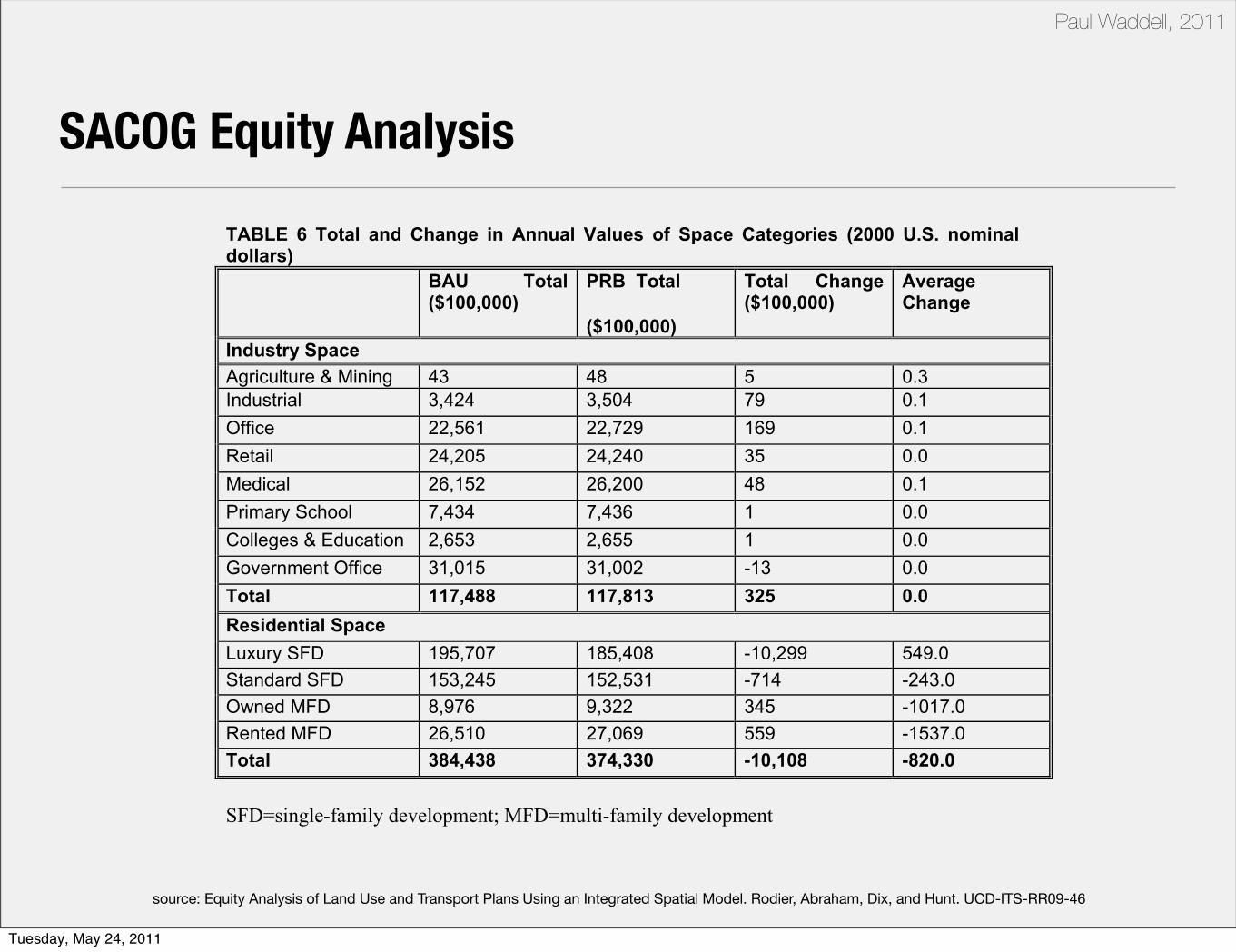
TABLE 6 Total and Change in Annual Values of Space Categories (2000 U.S. nominal dollars) BAU Total
($100,000) PRB Total
($100,000)
Total Change ($100,000)
Average Change
Industry Space Agriculture & Mining 43 48 5 0.3 Industrial 3,424 3,504 79 0.1 Office 22,561 22,729 169 0.1 Retail 24,205 24,240 35 0.0 Medical 26,152 26,200 48 0.1 Primary School 7,434 7,436 1 0.0 Colleges & Education 2,653 2,655 1 0.0 Government Office 31,015 31,002 -13 0.0 Total 117,488 117,813 325 0.0 Residential Space Luxury SFD 195,707 185,408 -10,299 549.0 Standard SFD 153,245 152,531 -714 -243.0 Owned MFD 8,976 9,322 345 -1017.0 Rented MFD 26,510 27,069 559 -1537.0 Total 384,438 374,330 -10,108 -820.0
SFD=single-family development; MFD=multi-family development
SACOG Equity Analysis
Tuesday, May 24, 2011
Paul Waddell, 2011
• California Statewide Integrated Model
• Integrated PECAS land use model and new statewide activity-based transportation model
• Spurred by California SB375: land use related reductions from autos and light trucks
• Funded by CalTrans in conjunction with metropolitan-level upgrades
• Massive data collection and imputation effort
• Timeline
- Transportation model built and calibrated during 2010
- Land use model calibration ongoing
- Metropolitan models ready by 2015
• Preliminary results
CalSIM
Tuesday, May 24, 2011

Paul Waddell, 2011
source: Developing California Integrated Land Use/Transportation Model. Gao, Lehmer, Wang, McCoy, Johnston, Abraham, and Hunt. Presented at TRB 2010
CalSIM
Tuesday, May 24, 2011
Paul Waddell, 2011
source: Developing California Integrated Land Use/Transportation Model. Gao, Lehmer, Wang, McCoy, Johnston, Abraham, and Hunt. Presented at TRB 2010
2
0
2
4
6
8
10
1 0 1 2 3 4 5 6 7 8 9
AGRICULTURE (Animals) PRODUCT
AGRICULTURE (Forestry and Fishing) PRODUCT
AGRICULTURE (Plants) PRODUCT
CONSTRUCTION (space) PRODUCT
HomeToOther
HomeToRec
HomeToShop
Labor
MANUFACTURING (Chemicals Plastic Rubber Glass Cement) PRODUCT
MANUFACTURING (Computers Electronics) PRODUCT
MANUFACTURING (Electrical Equipment Appliance) PRODUCT
MANUFACTURING (Food) PRODUCT
MANUFACTURING (Machinery) PRODUCT
MANUFACTURING (Metal Steel) PRODUCT
MANUFACTURING (Petro Coal production) PRODUCT
MANUFACTURING (Pulp and Paper) PRODUCT
MANUFACTURING (Textiles) PRODUCT
MANUFACTURING (Transportation Equipment) PRODUCT
MANUFACTURING (Wood Products Printing Furniture Misc) PRODUCT
MINING AND EXTRACTION PRODUCT
OtherToOther
OtherToRecreation
SCRAP
Transportation Comm Util and Wholesale
WorkToOther
Constrained 0 iteration model (supply/demand not matched)
CalSIM
Tuesday, May 24, 2011

Paul Waddell, 2011
source: Developing California Integrated Land Use/Transportation Model. Gao, Lehmer, Wang, McCoy, Johnston, Abraham, and Hunt. Presented at TRB 2010
CalSIM
Tuesday, May 24, 2011

Paul Waddell, 2011
source: Developing California Integrated Land Use/Transportation Model. Gao, Lehmer, Wang, McCoy, Johnston, Abraham, and Hunt. Presented at TRB 2010
Develop Target space quantity transitions10 counties selected to represent low med and high growth situations, plus San Francisco as a special county
Low: Sacramento, San Diego, Orange CountyMed: Amador, Inyo, ShastaHigh: Fresno, Imperial, PlacerSan Francisco
CalSIM
Tuesday, May 24, 2011

Paul Waddell, 2011
source: Developing California Integrated Land Use/Transportation Model. Gao, Lehmer, Wang, McCoy, Johnston, Abraham, and Hunt. Presented at TRB 2010
CalSIM
Tuesday, May 24, 2011
Paul Waddell, 2011
source: Developing California Integrated Land Use/Transportation Model. Gao, Lehmer, Wang, McCoy, Johnston, Abraham, and Hunt. Presented at TRB 2010
CalSIM
Tuesday, May 24, 2011
Paul Waddell, 2011
source: Developing California Integrated Land Use/Transportation Model. Gao, Lehmer, Wang, McCoy, Johnston, Abraham, and Hunt. Presented at TRB 2010
CalSIM
Tuesday, May 24, 2011
Paul Waddell, 2011
source: Developing California Integrated Land Use/Transportation Model. Gao, Lehmer, Wang, McCoy, Johnston, Abraham, and Hunt. Presented at TRB 2010
CalSIM
Tuesday, May 24, 2011

Paul Waddell, 2011
source: Developing California Integrated Land Use/Transportation Model. Gao, Lehmer, Wang, McCoy, Johnston, Abraham, and Hunt. Presented at TRB 2010
CalSIM
Tuesday, May 24, 2011

Paul Waddell, 2011
source: Developing California Integrated Land Use/Transportation Model. Gao, Lehmer, Wang, McCoy, Johnston, Abraham, and Hunt. Presented at TRB 2010
CalSIM
Tuesday, May 24, 2011

Paul Waddell, 2011
source: Developing California Integrated Land Use/Transportation Model. Gao, Lehmer, Wang, McCoy, Johnston, Abraham, and Hunt. Presented at TRB 2010
CalSIM
Tuesday, May 24, 2011

Paul Waddell, 2011
source: Developing California Integrated Land Use/Transportation Model. Gao, Lehmer, Wang, McCoy, Johnston, Abraham, and Hunt. Presented at TRB 2010
CalSIM
Tuesday, May 24, 2011

Paul Waddell, 2011
source: Developing California Integrated Land Use/Transportation Model. Gao, Lehmer, Wang, McCoy, Johnston, Abraham, and Hunt. Presented at TRB 2010
CalSIM
Tuesday, May 24, 2011
Paul Waddell, 2011
source: Developing California Integrated Land Use/Transportation Model. Gao, Lehmer, Wang, McCoy, Johnston, Abraham, and Hunt. Presented at TRB 2010
CalSIM
Tuesday, May 24, 2011
Paul Waddell, 2011
source: Developing California Integrated Land Use/Transportation Model. Gao, Lehmer, Wang, McCoy, Johnston, Abraham, and Hunt. Presented at TRB 2010
CalSIM
Tuesday, May 24, 2011

Paul Waddell, 2011
source: Developing California Integrated Land Use/Transportation Model. Gao, Lehmer, Wang, McCoy, Johnston, Abraham, and Hunt. Presented at TRB 2010
CalSIM
Tuesday, May 24, 2011

Paul Waddell, 2011
source: Developing California Integrated Land Use/Transportation Model. Gao, Lehmer, Wang, McCoy, Johnston, Abraham, and Hunt. Presented at TRB 2010
CalSIM
Tuesday, May 24, 2011
Paul Waddell, 2011
source: Developing California Integrated Land Use/Transportation Model. Gao, Lehmer, Wang, McCoy, Johnston, Abraham, and Hunt. Presented at TRB 2010
CalSIM
Tuesday, May 24, 2011
Paul Waddell, 2011
source: Developing California Integrated Land Use/Transportation Model. Gao, Lehmer, Wang, McCoy, Johnston, Abraham, and Hunt. Presented at TRB 2010
CalSIM
Tuesday, May 24, 2011

Paul Waddell, 2011
source: Developing California Integrated Land Use/Transportation Model. Gao, Lehmer, Wang, McCoy, Johnston, Abraham, and Hunt. Presented at TRB 2010
CalSIM
Tuesday, May 24, 2011
Paul Waddell, 2011
source: Developing California Integrated Land Use/Transportation Model. Gao, Lehmer, Wang, McCoy, Johnston, Abraham, and Hunt. Presented at TRB 2010
CalSIM
Tuesday, May 24, 2011

Paul Waddell, 2011
1. PECAS overview2. Anatomy of the System3. Application in Practice
4. Assessment
Tuesday, May 24, 2011
Paul Waddell, 2011
Strengths of Input-Output Models
• I-O Models provide a concise summary of the economic flows in the economy
• Multipliers from I-O models are used widely to predict the impact of changes in output of a sector on the broader economy - the multiplier effect
• With suitable data, national I-O models can be localized to states or possibly lower units of geography
- Keep in mind the model represents economic flows between every geographic unit and every sector, as in an international trade model - so the data requirements to generate a highly disaggregate I-O model are immense
Tuesday, May 24, 2011
Paul Waddell, 2011
Limitations of Input-Output Models
• Wikipedia’s article on Input-Output models provides the following assessment:
- “Input-output is conceptually simple. Its extension to a model of equilibrium in the national economy is also relatively simple and attractive but requires great skill and high-quality data. One who wishes to do work with input-output systems must deal skillfully with industry classification, data estimation, and inverting very large, ill-conditioned matrices. Moreover, changes in relative prices are not readily handled by this modeling approach alone.”
• I-O model theory does not account for the effects of changes in relative prices on production functions of firms, and therefore on the I-O structure
• I-O model does not allow flexible substitution among inputs and price adjustment
• I-O model deals only with monetary flows in the economy, not quantities of employment, households, population, etc.
• I-O model is an aggregate, static equilibrium model, with no capacity to represent effects of heterogeous agents, temporal dynamics, changes in production technology
Tuesday, May 24, 2011
Paul Waddell, 2011
• Built on a half-century of Input-Output modeling of macro-economies dating to Leontieff’s 1960’s model of U.S. economy, and spatial input-output models of MEPLAN and TRANUS from approximately 1970
• The spatial input-output framework has been used over several decades outside the U.S., and is beginning to see more use in the U.S., especially at a statewide scale
• Integrates interregional trade with and supports modeling of freight due to the relationship between trade and the movement of goods by mode at a time when logistics is becoming increasingly important in many cities
• The model development process can be started with IMPLAN, commercially available data that many U.S. regional planners already use
• Has been extended in PECAS to include not only origin and destination markets but also exchange markets
• Provides a static equilibrium framework, but can be run annually
• Is marketed as open source software (but not clear that it is downloadable)
Strengths of the PECAS Model System
Tuesday, May 24, 2011
Paul Waddell, 2011
Limitations of PECAS Model System
• Theory for price adjustment and its integration with I-O model needs development
• Spatial extensions to include production, consumption and exchange locations is complex and abstract
• Data is not readily available for the large number of assumptions to be made especially at the the metropolitan spatial scale, much must be synthesized.
• Creation of quantities of population, jobs, and commodity weights for freight movement are all derived by translating dollars flows to quantities
• AA module is an aggregate, static equilibrium model - not microsimulation
• SD module is a loosely coupled land transition model at a cell or parcel level, lacks demand side at comparable level of detail
• Model estimation/calibration is difficult and to our knowledge no applications have been developed without substantial consulting involvement by developers
• There is limited experience with fully operational applications. No MPOs had used PECAS for official Regional Transportation Plan updates in a 2010 survey by Maricopa Association of Governments; only one reported having used it in their projection series.
Tuesday, May 24, 2011

Questions and Discussion
PECAS Links:http://www.hbaspecto.com
Presenters:Paul WaddellDepartment of City and Regional PlanningUniversity of California Berkeleyemail: waddell at berkeley.edu
Mike ReillyAssociation of Bay Area Governmentsemail: michaelr at abag.ca.gov
Tuesday, May 24, 2011