Spatial Discrepancies between NHDPlus and LIDAR-Derived Stream Networks

University of Tennessee, KnoxvilleTrace: Tennessee Research and CreativeExchange

Masters Theses Graduate School

5-2012

Spatial Discrepancies between NHDPlus andLIDAR-Derived Stream NetworksNicole Marie [email protected]

This Thesis is brought to you for free and open access by the Graduate School at Trace: Tennessee Research and Creative Exchange. It has beenaccepted for inclusion in Masters Theses by an authorized administrator of Trace: Tennessee Research and Creative Exchange. For more information,please contact [email protected].

Recommended CitationSamu, Nicole Marie, "Spatial Discrepancies between NHDPlus and LIDAR-Derived Stream Networks. " Master's Thesis, University ofTennessee, 2012.https://trace.tennessee.edu/utk_gradthes/1202

https://trace.tennessee.edu

https://trace.tennessee.edu

https://trace.tennessee.edu/utk_gradthes

https://trace.tennessee.edu/utk-grad

mailto:[email protected]

To the Graduate Council:

I am submitting herewith a thesis written by Nicole Marie Samu entitled "Spatial Discrepancies betweenNHDPlus and LIDAR-Derived Stream Networks." I have examined the final electronic copy of thisthesis for form and content and recommend that it be accepted in partial fulfillment of the requirementsfor the degree of Master of Science, with a major in Geography.

Liem T. Tran, Major Professor

We have read this thesis and recommend its acceptance:

Carol P. Harden, Glenn A. Tootle

Accepted for the Council:Dixie L. Thompson

Vice Provost and Dean of the Graduate School

(Original signatures are on file with official student records.)

Spatial Discrepancies between NHDPlus and LIDAR-Derived Stream Networks

A Thesis Presented for the Master of Science

Degree The University of Tennessee, Knoxville

Nicole Marie Samu

May 2012

ii

Copyright 2012 by Nicole Marie Samu All rights reserved.

iii

Acknowledgements

I would like to thank Dr. Liem Tran for serving as my committee chair and for his resolute patience, encouragement, and guidance throughout my graduate school experience. I also thank my committee members, Drs. Carol Harden and Glenn Tootle, for helping me gain a better understanding of watershed processes and hydrology and for their support and guidance with my coursework and thesis. I greatly appreciate Dr. Yingkui Li for sharing his expertise in GIS and for the valuable learning experience that I had as his teaching assistant. I thank the Geographic Information Science and Technology Group at Oak Ridge National Laboratory for their support, words of wisdom, and encouragement over the years. I am eternally grateful for all of the coursework and thesis advice that I received from other graduate students. I am particularly in debt to Obeidillah Abdoul for helping me survive my hydrology engineering courses; to Pamela Dalal for sharing her wealth of knowledge about spatial statistics; and to Charlynn Burd for proofreading parts of my thesis. And finally, I thank my parents, Linda and Joe, my sister, Diane, and all of my friends and family for their unwavering support throughout this process.

iv

Abstract

Many organizations demand that current water resource issues necessitate improved stream network mapping for more accurate and reliable watershed analysis and modeling results, which can ultimately enable better management and policy decisions. Stream network data from the National Hydrography Dataset Plus (NHDPlus) and derived from Light Detection and Ranging (LIDAR) are each widely accepted to be of superior quality compared to many other conventional datasets. Each dataset indicates potential to improve a wide range of water resource applications; NHDPlus for its high spatial accuracy and functionality, and LIDAR-derived networks for their high resolutions. NHDPlus is publicly available and widely used; yet, until recently, high production costs and limited availability of LIDAR data have traditionally limited their widespread use in stream network mapping for water resource applications. However, recently increasing availability and decreasing costs suggest that LIDAR-derived networks could potentially be used to improve many application initiatives.

This study analyzes spatial discrepancies between NHDPlus and LIDAR-derived stream

network datasets. Results from analyses are intended to contribute information that can lead to improved stream network mapping and water resource applications. Mann-Whitney U and Wilcoxon-Signed Rank tests were first conducted to ascertain statistically significant types of spatial discrepancies existing between the datasets. Spatial autocorrelation analysis was then used to quantify spatial patterns of discrepancies between NHDPlus and LIDAR-derived networks. Next, Kruskal-Wallis tests were conducted to determine associations between local patterns of discrepancies and various landscape characteristics. Lastly, Spearman Rank Correlation tests were used to ascertain relationships between landscape characteristics and discrepancies between networks per catchment.

Results indicate that significant types and patterns of spatial discrepancies exist between NHDPlus and LIDAR-derived stream network datasets, and local patterns of the discrepancies are spatially related to various landscape characteristics. These findings imply how spatial discrepancies resulting between NHDPlus and LIDAR-derived networks may lead to differing watershed analysis and modeling results. Collectively, this research contributes building fundamental information for better understanding how to improve stream network mapping and water resource applications.

v

Table of Contents

Chapter Page

Chapter 1 Introduction ...................................................................................................................................................... 1

1.1 Problem Statement ................................................................................................................................................... 1

1.2 Research Questions and Hypotheses .................................................................................................................... 2

Chapter 2 Literature Review ............................................................................................................................................. 4

2.1 A Watershed Approach to Water Resource Initiatives ....................................................................................... 4

2.2 Stream Network Datasets and Watershed-based Decisions .............................................................................. 5

2.3 Characterizing Drainage Network Morphology .................................................................................................. 5

2.4 NHDPlus Stream Networks ................................................................................................................................... 7

2.5 DEM-derived Stream Networks ............................................................................................................................ 8

2.6 LIDAR-derived Stream Networks ......................................................................................................................... 9

Chapter 3 Study Areas ...................................................................................................................................................... 10

Chapter 4 Data and Methods .......................................................................................................................................... 12

4.1 Data Processing....................................................................................................................................................... 12

4.2 Determining Study Areas ...................................................................................................................................... 12

4.3 Automated Stream Network Extraction Process .............................................................................................. 12

4.4 Identifying Reach-Level Spatial Discrepancies .................................................................................................. 13

4.5 Identifying Catchment-Level Spatial Discrepancies .......................................................................................... 14

4.6 Spatial Autocorrelation Analysis .......................................................................................................................... 15

4.7 Relating Spatial Discrepancy Patterns to Landscape Characteristics ............................................................. 16

4.8 Spearman Rank Correlation Analysis .................................................................................................................. 17

Chapter 5 Results .............................................................................................................................................................. 19

5.1 Identifying Reach-Level Spatial Discrepancies .................................................................................................. 19

5.2. Identifying Catchment-Level Spatial Discrepancies ......................................................................................... 24

5.2.1 Total Stream Length per Catchment............................................................................................................. 25

5.2.2 Drainage Density per Catchment .................................................................................................................. 25

5.2.3 Reach Frequency per Catchment ................................................................................................................... 26

5.2.4 Mean Reach Length per Catchment ............................................................................................................. 26

5.3.1 Upper French Broad Watershed .................................................................................................................... 34

5.3.2 Rocky Watershed.............................................................................................................................................. 35

vi

5.3.3 Pamlico Watershed .............................................................................................................................................. 35

5.4 Spatial Discrepancy Patterns and Landscape Characteristics .......................................................................... 39

5.4.1 Total Stream Length Discrepancy Patterns ................................................................................................. 39

5.4.2 Drainage Density Discrepancy Patterns ....................................................................................................... 39

5.4.3 Reach Frequency Discrepancy Patterns ....................................................................................................... 40

5.4.4 Mean Reach Length Discrepancy Patterns .................................................................................................. 40

5.5 Spearman Rank Correlation Analysis Results .................................................................................................... 52

5.5.1 Total Stream Length per Catchment............................................................................................................. 52

5.5.2 Drainage Density per Catchment .................................................................................................................. 52

5.5.3 Stream Reach Frequency per Catchment ..................................................................................................... 53

5.5.4 Mean Stream Reach Length per Catchment ................................................................................................ 53

Chapter 6 Discussion and Conclusions ......................................................................................................................... 58

6.1 Discussion ................................................................................................................................................................ 58

6.2 Recommendations .................................................................................................................................................. 63

6.3. Conclusions ............................................................................................................................................................ 64

References .......................................................................................................................................................................... 66

Appendix ............................................................................................................................................................................ 70

Vita ...................................................................................................................................................................................... 77

vii

List of Tables

Table Page

Table 4.1. Classification of Land Cover Variables ....................................................................................................... 17

Table 5.1. Mann-Whitney U Tests of Reach Length Discrepancies Between LIDAR-derived and NHDPlus

Stream Network Datasets ............................................................................................................................................ 19

Table 5.2. Wilcoxon-Signed Rank Tests of Catchment-Level Spatial Discrepancies Between LIDAR-derived

and NHDPlus Stream Network Datasets ................................................................................................................. 25

Table 5.3. Kruskal-Wallis Tests based on Differences in Total Stream Length per Catchment between

LIDAR-derived and NHDPlus Datasets .................................................................................................................. 41

Table 5.4. Kruskal-Wallis Tests based on Differences in Drainage Density per Catchment between LIDAR-

derived and NHDPlus Datasets ................................................................................................................................. 42

Table 5.5. Kruskal-Wallis Tests based on Differences in Reach Frequency per Catchment between LIDAR-

derived and NHDPlus Datasets ................................................................................................................................. 43

Table 5.6. Kruskal-Wallis Tests based on Differences in Mean Reach Length per Catchment between

LIDAR-derived and NHDPlus Datasets .................................................................................................................. 44

Table 5.7. Spearman Rank Correlation Tests of Landscape Characteristics and Differences in Total Stream

Length per Catchment between LIDAR-derived and NHDPlus Stream Network Datasets .......................... 54

Table 5.8. Spearman Rank Correlation Tests of Landscape Characteristics and Differences in Drainage

Density per Catchment between LIDAR-derived and NHDPlus Stream Network Datasets ......................... 55

Table 5.9. Spearman Rank Correlation Analysis of Landscape Characteristics and Differences in Reach

Frequency per Catchment between LIDAR-derived and NHDPlus Stream Network Datasets..................... 56

Table 5.10. Spearman Rank Correlation Tests of Landscape Characteristics and Differences in Mean Reach

Length per Catchment between LIDAR-derived and NHDPlus Stream Network Datasets .......................... 57

Table A.1. Summary Statistics of LIDAR-derived and NHDPlus Reach-Level Stream Network Characteristics

.......................................................................................................................................................................................... 70

Table A.2. Summary Statistics of LIDAR-derived and NHDPlus Catchment-Level Stream Network

Characteristics: Upper French Broad Watershed ..................................................................................................... 71


Characteristics: Rocky Watershed............................................................................................................................... 72


Characteristics: Pamlico Watershed ........................................................................................................................... 73

Table A.5. Summary Statistics for Spatial Discrepancy Variables ............................................................................. 74

Table A.5. Continued. ...................................................................................................................................................... 75

Table A.6. Nonparametric Correlations of Landscape Characteristics and Catchment Areas ............................ 76

viii

List of Figures

Figure Page

Figure 2.1. Study Areas: Upper French Broad, Rocky, and Pamlico Watersheds .................................................. 10

Figure 4.1. Work Flow for Generating LIDAR-derived Stream Networks ....... Error! Bookmark not defined.

Figure 5.1. LIDAR-derived and NHDPlus Stream Network Datasets: Upper French Broad Study Area ........ 20

Figure 5.2. LIDAR-derived and NHDPlus Stream Network Datasets: Rocky Study Area.................................. 21

Figure 5.3. LIDAR-derived and NHDPlus Stream Network Datasets: Pamlico Study Area .............................. 22

Figure 5.4. Reach Lengths of LIDAR-derived and NHDPlus Stream Networks .................................................. 23

Figure 5.4. Continued. ...................................................................................................................................................... 24

Figure 5.5. Total Stream Length per Catchment Discrepancies between LIDAR-derived and NHDPlus

Stream Network Datasets ............................................................................................................................................ 27

Figure 5.6. Drainage Density per Catchment Discrepancies between LIDAR-derived and NHDPlus Stream

Network Datasets .......................................................................................................................................................... 28

Figure 5.7. Reach Frequency per Catchment Discrepancies between LIDAR-derived and NHDPlus Stream

Network Datasets .......................................................................................................................................................... 29

Figure 5.8. Mean Reach Length per Catchment Discrepancies between LIDAR-derived and NHDPlus Stream

Network Datasets ............................................................................................................................................................. 30

Figure 5.9. Discrepancies in Total Stream Length Per Catchment Between LIDAR-derived and NHDPlus

Datasets: Upper French Broad, Rocky, and Pamlico Drainage Areas ................................................................. 31

Figure 5.10. Discrepancies in Drainage Density Per Catchment Between LIDAR-derived and NHDPlus


Figure 5.11. Discrepancies in Reach Frequency Per Catchment Between LIDAR-derived and NHDPlus


Figure 5.12. Discrepancies in Mean Reach Length Per Catchment Between LIDAR-derived and NHDPlus


Figure 5.13. Spatial Autocorrelation Analysis of Spatial Discrepancies between LIDAR-derived and NHDPlus

Stream Networks in Upper French Broad Drainage Area ..................................................................................... 36


Stream Networks in Rocky Drainage Area ............................................................................................................... 37


Stream Networks in Pamlico Drainage Area ............................................................................................................ 38

Figure 5.16. Upper French Broad Watershed: Area, Canopy Coverage, and Slope Variables ............................. 45

Figure 5.17. Rocky Watershed: Area, Canopy Coverage, and Slope Variables ....................................................... 46

Figure 5.18. Pamlico Watershed: Area, Canopy Coverage, and Slope Variables .................................................... 47

ix

Figure 5.19. Upper French Broad Watershed: Variables Showing Proportions of Land Cover Types Per

Catchment ...................................................................................................................................................................... 48

Figure 5.20. Rocky Watershed: Variables Showing Proportions of Land Cover Types Per Catchment ............ 49

Figure 5.21. Pamlico Watershed: Variables Showing Proportions of Land Cover Types Per Catchment ......... 50

Figure 5.22. Aspect per Catchment: Upper French Broad, Rocky, and Pamlico Watersheds ............................. 51

1

Chapter 1 Introduction

1.1 Problem Statement

The primary objective of this research is to analyze spatial discrepancies between NHDPlus and LIDAR-derived stream network datasets. This fundamental step in data collection and extrapolation is a cornerstone for improved watershed management and policy decisions. Two types of high quality stream network datasets, LIDAR-derived and NHDPlus networks, are compared in this study to take a step toward better understanding their spatial discrepancies and associated implications for water resource initiatives.

Progress has been made in water resource management and planning. However, ongoing efforts to improve watershed analyses and modeling are critical for sustainable management and optimization of a wide range of ecosystem services delivered to humans and the environment. Examples of these initiatives include the provision of clean drinking water, flood control, drought mitigation, and the protection of aquatic and terrestrial biodiversity.

Successful watershed analysis and modeling requires stream network datasets to comprise spatial representations that sufficiently account for natural flow paths draining earth’s surface and reflect the morphologic characteristics of networks as they occur in nature. Insufficient spatial depictions of stream networks could bring about incorrect and ambiguous analysis results, producing false implications, which can potentially lead to poor water resource management and policy decisions. In particular, there has been much recent interest by various organizations in improving the spatial accuracy and classification of upstream waters. Producing adequate spatial representations of headwaters, especially ephemeral streams, is a recurring challenge in stream network mapping.

Improvements to water resource applications necessitate continued research efforts toward better understanding how different data or resolutions used in stream network mapping will lead to different analysis results. A growing body of work provides evidence of how landscape characteristics such as slope, vegetation density, aspect, impervious surfaces, soils, geology, and stream channel morphology have been empirically linked to spatial differences between stream network datasets generated at different spatial scales, and/or produced from different sources, methods, and measurement schemes (e.g. Gyasi-Agyei et al. 1995; Barber and Shortridge, 2005; James et al. 2007; Li and Wong, 2009; Zhao et al. 2009). However, current literature warrants a more comprehensive and in-depth empirical understanding of relationships between landscape characteristics and spatial discrepancies among stream network datasets. Studies indicate that spatial discrepancies exist between LIDAR-derived and NHDPlus networks because of the different ways in which they are generated.

Stream network data from the National Hydrography Dataset Plus (NHDPlus) and derived from Light Detection and Ranging (LIDAR) have demonstrable potential to improve stream network mapping and therefore impact a broad range of water resource initiatives. Advantages of using NHDPlus data are the following: publicly available, commonly used, have continuous spatial coverage of the United States, and superior spatial accuracies compared to many other high quality conventional datasets. Advantages of using LIDAR technologies to construct stream networks are the following: efficient delineation methods and finely spaced point cloud data to extrapolate high-

2

resolution terrain relief. The merits of NHDPlus and LIDAR datasets are well documented. These data sources supply a superior spatial detail and accuracy (e.g. James et al. 2007; Zhao et al. 2008; and Li and Wong, 2010) when compared to other data sources.

Although LIDAR-derived stream network datasets have been used in various important water resource initiatives and their potential capabilities have been well-recognized in literature, LIDAR-derived networks have yet to become standard datasets in watershed analysis and modeling due to concern about high production costs and limited availability. However, recently decreasing production costs and increasing availability of high-resolution LIDAR data show increasing potential to improve various water resource applications.

In this thesis, metrics adopted or customized from applied hydrology and geostatistics are used to derive reach and catchment-level variables to elucidate spatial discrepancies between LIDAR-derived and NHDPlus stream network datasets and to analyze relationships between landscape characteristics and the spatial discrepancies. The analyses are conducted on three comparable scale watersheds of differing physiographies to highlight how spatial discrepancies between the datasets vary between watersheds with highly different landscape characteristic patterns. The watersheds selected for analyses include the North Carolina portion of the French Broad Watershed, the Rocky Watershed in North Carolina, and the Pamlico Watershed in North Carolina. The French Broad study area falls within the Blue Ridge Physiographic Province which comprises a mostly rugged mountainous and highly forested landscape. In contrast, Rocky Watershed contains gently rolling hills and land use strongly dominated by agriculture. The Pamlico Watershed falls within the Coastal Plain physiographic region, which is extremely flat and largely intersected by vast wetlands.

Analyses conducted in this thesis compare spatial differences between LIDAR-derived and NHDPlus stream network datasets. ArcGIS 10 geoprocessing tools and functionalities (ESRI, 2010) are used to assemble, process, and visualize data and analysis results. Also, Microsoft Excel, SPSS 20, and GeoDa software are used to facilitate in data management, and processing.

Results presented in this study contribute building an understanding of spatial discrepancies between LIDAR-derived and NHDPlus stream network datasets. The methods employed here are fundamental in refining end users’ knowledge and highlighting the limitations or advantages of each. Discerning similarities and differences between the two datasets will help researchers and users to best select appropriate data for analysis that is appropriate for the location and scale of modeling, thereby yielding a greater impact on water resource applications.

1.2 Research Questions and Hypotheses

The main objective of this thesis is to analyze the spatial discrepancies between NHDPlus and LIDAR-derived stream networks datasets. To accomplish this goal, research methods were designed and implemented to address the following research questions:

1. What types of spatial discrepancies exist between NHDPlus stream networks and networks derived from LIDAR data?

2. What are the spatial patterns of discrepancies between LIDAR-derived and NHDPlus networks?

3

3. How are landscape characteristics related to the spatial discrepancies between NHDPlus and LIDAR-derived stream network datasets?

My hypotheses include:

1. Significant discrepancies in stream reach lengths exist between NHDPlus and LIDAR-derived stream networks.

2. High resolution of LIDAR-derived DEMs allows for LIDAR-derived stream networks to contain greater spatial detail than NHDPlus networks.

3. Spatial patterns of discrepancies significantly differ among watersheds of comparable scales but differing physiographies.

4. There are associations between spatial patterns of discrepancies and landscape characteristics.

5. Strong correlations exist between spatial discrepancy values and catchment area, canopy coverage, and slope.

4

Chapter 2 Literature Review

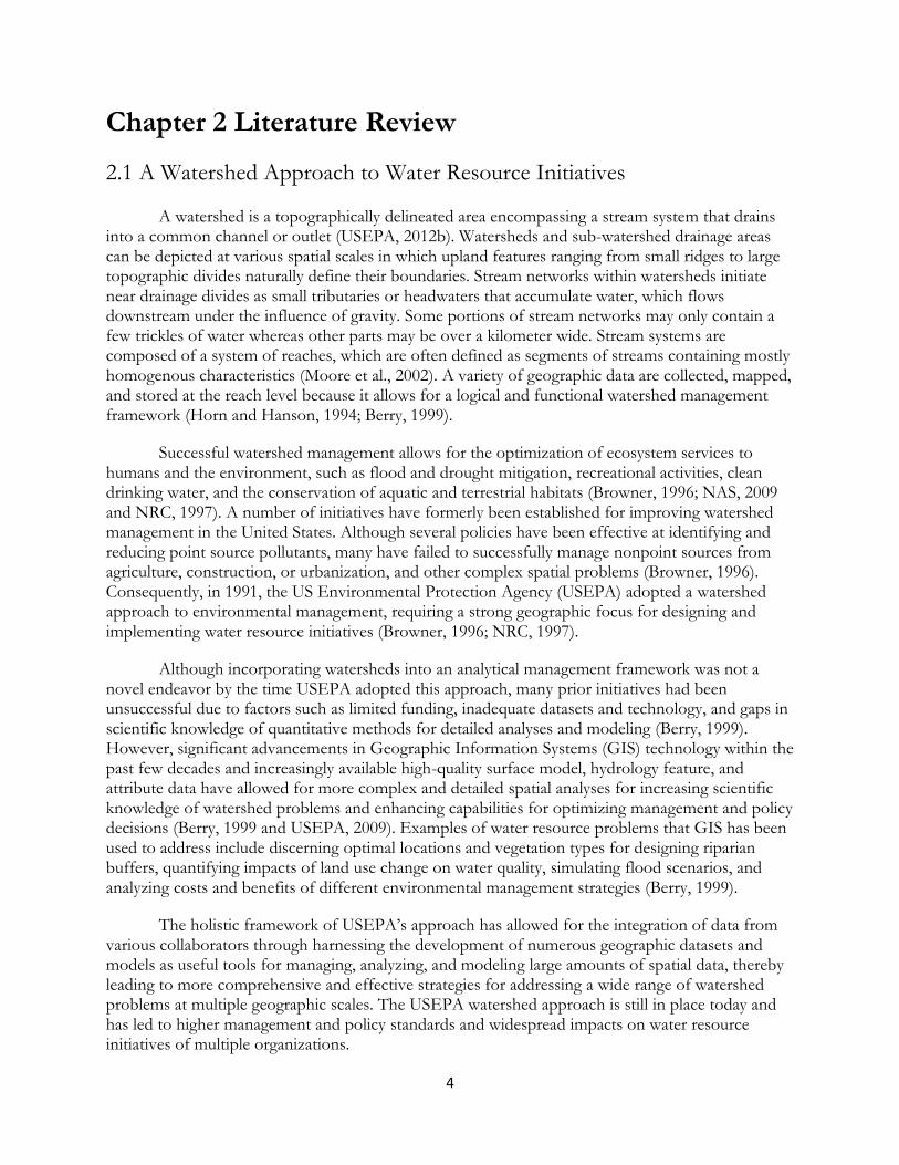
2.1 A Watershed Approach to Water Resource Initiatives

A watershed is a topographically delineated area encompassing a stream system that drains into a common channel or outlet (USEPA, 2012b). Watersheds and sub-watershed drainage areas can be depicted at various spatial scales in which upland features ranging from small ridges to large topographic divides naturally define their boundaries. Stream networks within watersheds initiate near drainage divides as small tributaries or headwaters that accumulate water, which flows downstream under the influence of gravity. Some portions of stream networks may only contain a few trickles of water whereas other parts may be over a kilometer wide. Stream systems are composed of a system of reaches, which are often defined as segments of streams containing mostly homogenous characteristics (Moore et al., 2002). A variety of geographic data are collected, mapped, and stored at the reach level because it allows for a logical and functional watershed management framework (Horn and Hanson, 1994; Berry, 1999).

Successful watershed management allows for the optimization of ecosystem services to humans and the environment, such as flood and drought mitigation, recreational activities, clean drinking water, and the conservation of aquatic and terrestrial habitats (Browner, 1996; NAS, 2009 and NRC, 1997). A number of initiatives have formerly been established for improving watershed management in the United States. Although several policies have been effective at identifying and reducing point source pollutants, many have failed to successfully manage nonpoint sources from agriculture, construction, or urbanization, and other complex spatial problems (Browner, 1996). Consequently, in 1991, the US Environmental Protection Agency (USEPA) adopted a watershed approach to environmental management, requiring a strong geographic focus for designing and implementing water resource initiatives (Browner, 1996; NRC, 1997).

Although incorporating watersheds into an analytical management framework was not a novel endeavor by the time USEPA adopted this approach, many prior initiatives had been unsuccessful due to factors such as limited funding, inadequate datasets and technology, and gaps in scientific knowledge of quantitative methods for detailed analyses and modeling (Berry, 1999). However, significant advancements in Geographic Information Systems (GIS) technology within the past few decades and increasingly available high-quality surface model, hydrology feature, and attribute data have allowed for more complex and detailed spatial analyses for increasing scientific knowledge of watershed problems and enhancing capabilities for optimizing management and policy decisions (Berry, 1999 and USEPA, 2009). Examples of water resource problems that GIS has been used to address include discerning optimal locations and vegetation types for designing riparian buffers, quantifying impacts of land use change on water quality, simulating flood scenarios, and analyzing costs and benefits of different environmental management strategies (Berry, 1999).

The holistic framework of USEPA’s approach has allowed for the integration of data from various collaborators through harnessing the development of numerous geographic datasets and models as useful tools for managing, analyzing, and modeling large amounts of spatial data, thereby leading to more comprehensive and effective strategies for addressing a wide range of watershed problems at multiple geographic scales. The USEPA watershed approach is still in place today and has led to higher management and policy standards and widespread impacts on water resource initiatives of multiple organizations.

5

2.2 Stream Network Datasets and Watershed-based Decisions

Stream network datasets have become essential components of today’s watershed-based management and decision making. Within recent decades, increasing availability and functionality of GIS software and data and the integration of GIS and hydrologic modeling systems have facilitated stream network dataset capabilities to extend from description to prediction and to optimization for multi-domain water resource initiatives (Berry, 1999). Today’s conventional stream network data models used in watershed analysis and modeling have largely evolved under the broad interdisciplinary umbrella of geomorphometry, which integrates concepts and applications from mathematics, earth science, engineering, and computer science (Pike, 2009).

Geomorphometry can be described as “the morphometry of landforms with or without digital data” (Pike et al., 2009), which collectively involves the use of established metrics for quantitatively characterizing and understanding the physical landscape at various spatial scales. Quantitative evaluation of drainage areas and the advent of GIS technologies have collectively allowed for the development of several types of geographic datasets used today for a wide range of applications, such as cost-benefit analyses of watershed management approaches, climate modeling, water quality monitoring and hydrologic simulations, precision agriculture, urban planning, education, and human-environmental vulnerability and risk analyses (Browner, 1996; NRC, 1997; Pike et al., 2009).

2.3 Characterizing Drainage Network Morphology

Since the classification of stream network features in geographic datasets provides a foundation for watershed analysis, it is important for features to be appropriately classified to provide appropriate spatial representations of surface drainage paths as they occur in nature. A large body of work has contributed to the quantitative classification of drainage networks for improving stream network datasets and their use in various applications. Much impetus for the development of quantitative methods for characterizing networks was initially spurred through Horton’s (1945) synthesis of methods for characterizing drainage morphology and erosional processes. Significant work followed in building a quantitative basis for drainage network analysis.

Contributions from Strahler (1952) and Shreve (1966) in the hierarchical classification of streams led to significant developments in the characterizations of drainage networks leading to considerable progress in watershed analysis. Notable early developments were also spurred from findings of Morisawa (1962) in which she suggests that quantitative methods for characterizing watershed morphologies may potentially be useful for practical purposes. Since then, a large body of work has reconfirmed Morisawa’s findings and their significance for addressing various water resource issues (e.g. Ogunkoya et al., 1983; Pitlick, 1994; Ifabiyi, 2004; Jimoh-Iroye, 2010).

This growing body of work underscores the general importance of producing spatially complete and accurate stream network datasets and has influenced the development of widespread water resource applications used today. Effective water resource applications require stream network datasets comprising networks that are spatially characteristic of surface drainage paths occurring in nature. Typically, the fundamental accounting unit of conventional stream network datasets is the reach feature. Appropriately classifying reach features is important as they provide a framework for indicating changes in the physical and chemical compositions of streams (Horn and Hanson, 1994;

6

Moore et al., 2002; Alexander et al., 2007). In nature, interactions between earth’s land, water, and climate systems cause the physical and chemical compositions of streams to be continuously altered. As a result, sufficiently characterizing stream network datasets both spatially and temporally has traditionally been a challenge.

2.3.1 Stream Morphology Metrics and Hydrologic Implications

Drainage density (D) has been extensively used as a metric for watershed analyses. D was defined by Horton (1945) as the average length of streams per unit area, and describes “the linear scale of landforms in fluvially eroded landscapes” (Abrahams and Ponczynski, 1984). D can be both directly and indirectly statistically related to water quantity and quality parameters (Bloschl, 2008; Merz and Bloschl, 2008; Pallard et al., 2009). Generally, direct effects refer to explicit relationships between D and water quantity (e.g. peak flood magnitude, mean runoff) and quality (e.g. suspended sediment yield, nitrogen load) indicators, and indirect effects consider implicit connections between D and water quantity and quality variables modulated by land (e.g. geology, soil, land use) and climate (e.g. precipitation, temperature, humidity) factors (Bloschl, 2008; Merz and Bloschl, 2008; Pallard et al., 2009).

D has been quantitatively shown to reflect climate and topography in a number of different ways. Abrahams and Ponczynski (1984) showed how precipitation (PM) and precipitation intensity (PI) can either be positively or inversely related to D, and either allow for an increase or decrease in surface runoff. They concluded that PM and PI control D by either increasing vegetation growth and soil depth, leading to higher soil infiltration rates and ground resistance to erosion, thus lower densities and decreased runoff intensity; or increasing D by increasing soil impacts and erosion rates (channel incision) leading to greater runoff intensity. D is typically higher in arid locations with sparse vegetation and directly increases with higher PM and PI (Abrahams and Ponczynski, 1984; Brookfield, 1966; Gregory, 1977; Woodyer, 1968). D has also been linked to geologic characteristics of watersheds. For example, reduced D may be attributed to increased rocky slopes, impervious surfaces, karst landscapes or highly weathered bedrock (Pallard et al., 2008)

Studies show that high D is associated with increased water quantity estimates. Authors have suggested that higher D implies streams are closer together thus overland travel time is lower for water to reach streams (Gregory and Walling, 1973; Ogunkoya et al., 1984; and Preston et al., 1998), allowing for less probability of surface runoff being lost to evapotranspiration (Ogunkoya et al., 1984). Consequently, increased runoff leads to increased in-stream flow volumes, which flow at higher velocities within networks and lead to higher peak flow magnitudes (Pallard et al., 2008).

D is often regarded as one of the most important drainage network characteristics used for quantifying drainage network morphologies and indicating watershed processes. However, sufficient evaluations of networks necessitate analyzing more factors than just D alone. Stream length (L) is also important for watershed analyses and modeling. Particularly, L implies in-stream flow times. Given L, the average cross-sectional area of a stream, a coefficient to correct for different flow velocities of the surface and bed of the stream, and the time for a float to travel from one point of a stream to another; in-stream flows can be calculated (USEPA, 2012a). Further, increased runoff leads to increased in-stream flow volumes, which flow at higher velocities within networks and lead to higher peak flow magnitudes (Pallard et al., 2008).

7

Analyzing stream frequency (F) can also lead to important information that can be useful toward improving water quantity and quality related applications. Horton (1945) defines stream frequency as the number of streams per unit area. F patterns signify connectivity of streams throughout drainage networks, which implies changes in the physical and chemical conditions of water (Dodds and Rothman, 2000; Alexander et al. 2007). In addition, as inferred from Horton’s (1945) law of stream numbers, F is relevant to the numbers of stream reaches from one stream order to the next or the ‘bifurcation ratio,’ indicating that F is linked to patterns of drainage densities.

2.4 NHDPlus Stream Networks

NHDPlus is an integrated collection of geospatial data that extend capabilities and functionality of the NHD dataset. NHDPlus is comprised of various key features from the NHD, National Elevation Dataset (NED), National Watershed Boundary Dataset (WBD), as well as other attributes (USEPA and USGS, 2010). Its hydrographic model framework includes continuous coverage of the United States and stream networks are based off of NHD flowlines, which are a set of spatially referenced linear features linking to form a system of reaches and routes (USEPA and USGS, 2010).

An NHDPlus reach is a spatially defined, addressable unit which can be a stream, waterbody, or coastline feature. Chains of reaches in NHDPlus are indexed along spatially referenced routes and addressed proportionally from 0 to one 100 along each route. Discrete locations and events have been linked to reach features in NHDPlus for improved navigation and application-ready analysis and modeling (McKay, 2008).

The NHDPlus data also contains drainage area features ranging from the catchment-level to regional scale. Hydrologic features contain unique IDs that allow for complex data integration for a wide range of analysis and modeling at various spatial scales. In addition, NHDPlus includes datasets such as NHD hydro-enforced flow direction and accumulation grids, and stream flow volume and velocity estimates (USEPA and USGS, 2010). Public availability and robust application-ready functionalities of NHDPlus facilitate its widespread use toward various watershed initiatives.

Although applications of NHDPlus stream network data have shown to be highly effective, further research is required to better understand how NHDPlus differs from stream network datasets derived from surface elevation data such as digital elevation models (DEM) or networks derived from light detection and ranging data (LIDAR), and how relative discrepancies may affect implications of various hydrologic analysis and modeling applications A comparison between NHDPlus and LIDAR-derived datasets may potentially allow for a clearer understanding of how the delineation of stream network datasets may differ spatially due to different data sources, measurement scales, collection techniques, and processing methods. In particular, an analysis of the relationships between landscape characteristics and spatial discrepancies between the datasets may contribute useful insights for certain types of commonly used publicly available stream network datasets and their corresponding impacts on applications.

Certain aspects of NHDPlus stream network processing methods imply spatial patterns of discrepancies that may exist between NHDPlus and networks extracted using automated techniques. In particular, streams of NHDPlus networks are generated from multiple editors digitizing streams from various topographic map sources, comprising inconsistent spatial scales (McKay, 2008; USGS, 1998). The nature of this approach leads to challenges in accurately depicting and consistently

8

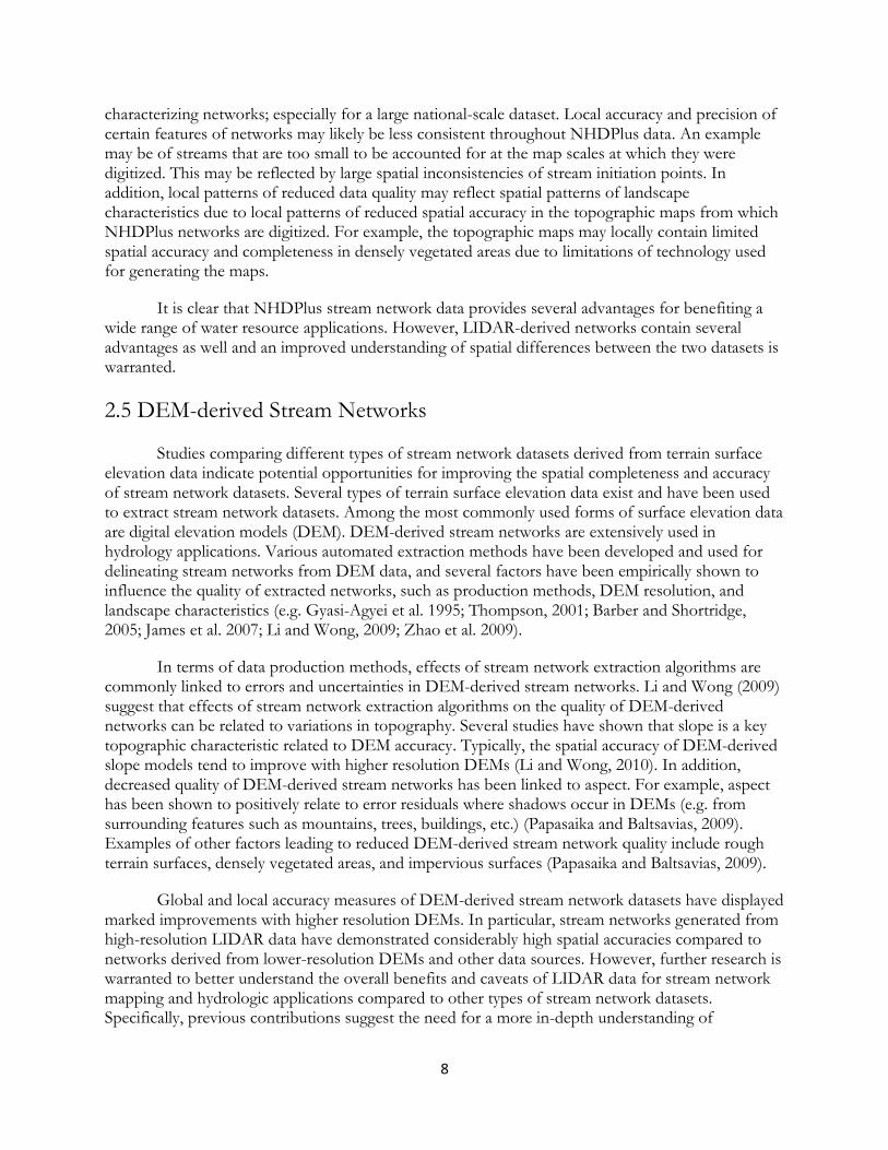
characterizing networks; especially for a large national-scale dataset. Local accuracy and precision of certain features of networks may likely be less consistent throughout NHDPlus data. An example may be of streams that are too small to be accounted for at the map scales at which they were digitized. This may be reflected by large spatial inconsistencies of stream initiation points. In addition, local patterns of reduced data quality may reflect spatial patterns of landscape characteristics due to local patterns of reduced spatial accuracy in the topographic maps from which NHDPlus networks are digitized. For example, the topographic maps may locally contain limited spatial accuracy and completeness in densely vegetated areas due to limitations of technology used for generating the maps.

It is clear that NHDPlus stream network data provides several advantages for benefiting a wide range of water resource applications. However, LIDAR-derived networks contain several advantages as well and an improved understanding of spatial differences between the two datasets is warranted.

2.5 DEM-derived Stream Networks

Studies comparing different types of stream network datasets derived from terrain surface elevation data indicate potential opportunities for improving the spatial completeness and accuracy of stream network datasets. Several types of terrain surface elevation data exist and have been used to extract stream network datasets. Among the most commonly used forms of surface elevation data are digital elevation models (DEM). DEM-derived stream networks are extensively used in hydrology applications. Various automated extraction methods have been developed and used for delineating stream networks from DEM data, and several factors have been empirically shown to influence the quality of extracted networks, such as production methods, DEM resolution, and landscape characteristics (e.g. Gyasi-Agyei et al. 1995; Thompson, 2001; Barber and Shortridge, 2005; James et al. 2007; Li and Wong, 2009; Zhao et al. 2009).

In terms of data production methods, effects of stream network extraction algorithms are commonly linked to errors and uncertainties in DEM-derived stream networks. Li and Wong (2009) suggest that effects of stream network extraction algorithms on the quality of DEM-derived networks can be related to variations in topography. Several studies have shown that slope is a key topographic characteristic related to DEM accuracy. Typically, the spatial accuracy of DEM-derived slope models tend to improve with higher resolution DEMs (Li and Wong, 2010). In addition, decreased quality of DEM-derived stream networks has been linked to aspect. For example, aspect has been shown to positively relate to error residuals where shadows occur in DEMs (e.g. from surrounding features such as mountains, trees, buildings, etc.) (Papasaika and Baltsavias, 2009). Examples of other factors leading to reduced DEM-derived stream network quality include rough terrain surfaces, densely vegetated areas, and impervious surfaces (Papasaika and Baltsavias, 2009).

Global and local accuracy measures of DEM-derived stream network datasets have displayed marked improvements with higher resolution DEMs. In particular, stream networks generated from high-resolution LIDAR data have demonstrated considerably high spatial accuracies compared to networks derived from lower-resolution DEMs and other data sources. However, further research is warranted to better understand the overall benefits and caveats of LIDAR data for stream network mapping and hydrologic applications compared to other types of stream network datasets. Specifically, previous contributions suggest the need for a more in-depth understanding of

9

connections between landscape characteristics and spatial discrepancies between stream network datasets. This knowledge is particularly relevant considering the decreasing costs, increasing public availability, and demonstrated potential of LIDAR data (Li and Wong, 2009).

2.6 LIDAR-derived Stream Networks

Most conventional DEM sources such as NED or the Shuttle Radar Topography Mission (SRTM) dataset are generated from passive remote sensing technologies, which capture information through aerial photogrammetric technologies that measure naturally occurring energy reflected from the earth’s surface, typically from the sun (NOAA, 2009; NASA, 2011; USGS, 2011). In contrast, LIDAR is a type of active remote sensing technology that uses a Global Positioning System (GPS), Inertial Navigation System (INS), and lasers to develop high-resolution topographic data of large areas (James at al., 2007; Terrapoint, 2008). LIDAR data are collected through emitting an array of laser pulses from an aircraft or ground unit in which the time between the emission of pulses emitted and receipt of return signals from reflected energy is converted to distance through a ranging unit (James et al., 2007). Return signals correspond successively to the locations of surfaces that they contact. For example, LIDAR-derived surface elevation models generated from first return signals commonly capture surfaces of tree canopies or spatial footprints of building tops, whereas the earth’s ground surface would be generated from last returns. The raw data consists of dense point clouds in which individual points correspond to the precise geographic coordinates of reflected surfaces. Processing of last return signals to generate terrain surface models entails applying interpolation techniques for producing continuous surface representations of data, and additional computational methods are applied for removing vegetation and artifacts (e.g. extraneous features such as buildings, bridges, or culverts).

Studies show that LIDAR technology is capable of improving mapping of stream networks depending on the distribution and density of laser pulses emitted and processing methods used for deriving the networks. Results from James et al. (2007) show that LIDAR is the best available technology for mapping highly accurate depictions of gully and headwater networks in densely forested locations, except where streams are relatively narrow or parallel and closely spaced. Similarly, Zhao et al. (2010) compared 1 and 10 m LIDAR-derived DEMs, and a conventional 10 m DEM derived from aerial photogrammetry, and found that the 1 m resolution DEMs derived from LIDAR performed substantially better at mapping flow diversion terrace failures.

Conversely, LIDAR technologies emitting moderate laser scans over densely forested areas can produce significantly poor quality data and occasionally even large data gaps as a result of sparse point cloud spacing of the terrain surface. Problems can also arise from overly dense point cloud spacing. If data are not carefully processed to remove artifacts, LIDAR-derived DEMs can produce greatly distorted landscape features and lead to incorrect results of various applications. Other known caveats of LIDAR can occur from many geoprocessing algorithms that have not yet been extended to handle datasets containing resolutions as high as LIDAR-derived DEMs. These types of problems have commonly been shown to occur with stream network extraction algorithms (Garcia, 2004). Examples of some resulting issues include abundances of sinks in LIDAR-derived DEMs and artificial channels delineated in areas containing braided streams, wide channels, and various types of anthropogenic features.

10

Chapter 3 Study Areas

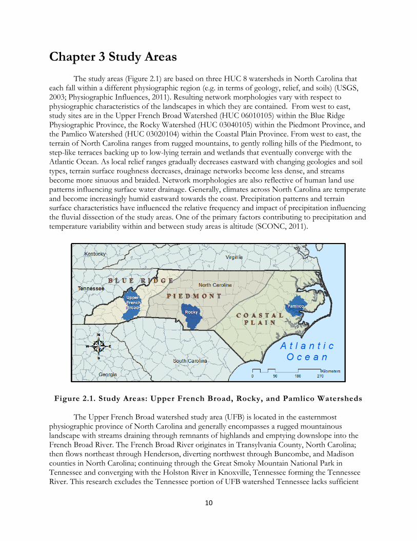
The study areas (Figure 2.1) are based on three HUC 8 watersheds in North Carolina that each fall within a different physiographic region (e.g. in terms of geology, relief, and soils) (USGS, 2003; Physiographic Influences, 2011). Resulting network morphologies vary with respect to physiographic characteristics of the landscapes in which they are contained. From west to east, study sites are in the Upper French Broad Watershed (HUC 06010105) within the Blue Ridge Physiographic Province, the Rocky Watershed (HUC 03040105) within the Piedmont Province, and the Pamlico Watershed (HUC 03020104) within the Coastal Plain Province. From west to east, the terrain of North Carolina ranges from rugged mountains, to gently rolling hills of the Piedmont, to step-like terraces backing up to low-lying terrain and wetlands that eventually converge with the Atlantic Ocean. As local relief ranges gradually decreases eastward with changing geologies and soil types, terrain surface roughness decreases, drainage networks become less dense, and streams become more sinuous and braided. Network morphologies are also reflective of human land use patterns influencing surface water drainage. Generally, climates across North Carolina are temperate and become increasingly humid eastward towards the coast. Precipitation patterns and terrain surface characteristics have influenced the relative frequency and impact of precipitation influencing the fluvial dissection of the study areas. One of the primary factors contributing to precipitation and temperature variability within and between study areas is altitude (SCONC, 2011).

Figure 2.1. Study Areas: Upper French Broad, Rocky, and Pamlico Watersheds The Upper French Broad watershed study area (UFB) is located in the easternmost

physiographic province of North Carolina and generally encompasses a rugged mountainous landscape with streams draining through remnants of highlands and emptying downslope into the French Broad River. The French Broad River originates in Transylvania County, North Carolina; then flows northeast through Henderson, diverting northwest through Buncombe, and Madison counties in North Carolina; continuing through the Great Smoky Mountain National Park in Tennessee and converging with the Holston River in Knoxville, Tennessee forming the Tennessee River. This research excludes the Tennessee portion of UFB watershed Tennessee lacks sufficient

11

available data for analyses (USEPA and USGS, 2010). Land cover within the UFB study area ranges from vast wilderness of the Pisgah National Forest, to sparsely-populated agricultural and manufacturing communities, such as the city of Brevard in Transylvania County; to more developed land such as the city of Ashville (Columbia Gazetteer of the World Online s.v. “Brevard.” Accessed from: http://www.columbiagazetteer.org/main/ViewPlace/19162 October 2011).

The Rocky watershed study area (ROC) is located in south-central North Carolina within the older non-mountainous portion of the Appalachians, which is largely underlain by crystalline rock and consists mainly of gently rolling hills dissected by channels forming steep valleys (Physiographic Influences, 2011). The watershed drains into the Rocky River, which originates in Iredell County, and descends southeastward for approximately 145 km, passing through Kannapolis and Concord and converging with the Yadkin River to form the Pee Dee River (Columbia Gazetteer of the World Online s.v. “Rocky River.” Accessed from: October 2011). The area is sparsely populated and consists mainly of forest and agricultural land. Urbanized areas are primarily only concentrated in the Liberty area, around Siler City, and scattered along major transportation routes (TLC, 2011).

The Pamlico study area (PAM) lies along the central coast of North Carolina, predominantly in

Beaufort County. The watershed area comprises very flat low-relief terrain consisting primarily of

row-crop agriculture and forests interspersed by vast wetlands. Various portions of the watershed

also include artificially implanted drainage features such as irrigation ditches and canals. Most of the

developed land exists near Washington (NC DWQ, 2010). The watershed drains into the Pamlico

River, which extends from the town of Washington to Roos Point (NC DWQ, 2010). The Pamlico

River widens eastward into an expansive estuary system emptying into Pamlico Sound to the east.

The Tar River flows into the Pamlico River from the West and several arms converge with the

Pamlico River eastward from the north and south, one of the largest being the Pungo River.

(Columbia Gazetteer of the World Online “Pamlico River.” Accessed from:

http://www.columbiagazeteer.org/main/ViewPlace/119557 October 2011).

http://www.columbiagazetteer.org.proxy.lib.utk.edu:90/main/ViewPlace/19162

12

Chapter 4 Data and Methods

4.1 Data Processing

Reach and catchment-levels datasets were prepared to analyze spatial discrepancies between LIDAR-derived and NHDPlus networks for the study areas. Geoprocessing methods in ArcGIS 10 software (ESRI, 2010) were used to generate stream networks from LIDAR for the study areas using 1/9 arc second resolution NED data. Resulting LIDAR-derived and NHDPlus stream network datasets contained spatially referenced systems of reaches for each of the study areas and individual lengths of reaches were calculated in meters. Reach and catchment-level variables were derived to analyze spatial patterns of discrepancies between the datasets and their relationships with landscape characteristics for watersheds of comparable scales and differing physiographies.

4.2 Determining Study Areas

Study areas were largely determined based on the availability of data. Dense raw point cloud LIDAR data (unprocessed) are publicly available for most of North Carolina; yet, it was concluded that the higher amount of detail that may potentially be achieved through deriving stream networks from unprocessed LIDAR would likely not outweigh the required time and effort to extract reasonably accurate datasets for analyses. Alternatively, networks were derived from pre-processed LIDAR data available in the form of high-resolution DEMs. The DEMs are 1/9 arc second resolution data from the National Elevation Dataset (NED). This resolution of NED data is primarily generated from LIDAR, which is likely why they are commonly referred to in literature as one of the highest resolution publicly available DEM datasets. Publicly available 1/9 arc second NED data are not yet widely available in the US. Therefore, study areas were selected from North Carolina because the available data were most suitable for this research.

Three HUC 8 drainage areas were selected from within different physiographic provinces in North Carolina. The UFB drainage area contains land in Tennessee and North Carolina, but only the North Carolina portion was used for analyses because data were not available for the Tennessee portion. Once HUC 8 watershed areas were selected, their boundaries were then corrected to spatially align with NHDPlus catchment shapefiles.

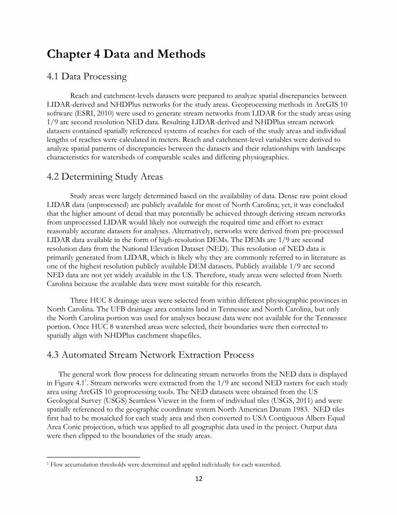
4.3 Automated Stream Network Extraction Process

The general work flow process for delineating stream networks from the NED data is displayed in Figure 4.11. Stream networks were extracted from the 1/9 arc second NED rasters for each study area using ArcGIS 10 geoprocessing tools. The NED datasets were obtained from the US Geological Survey (USGS) Seamless Viewer in the form of individual tiles (USGS, 2011) and were spatially referenced to the geographic coordinate system North American Datum 1983. NED tiles first had to be mosaicked for each study area and then converted to USA Contiguous Albers Equal Area Conic projection, which was applied to all geographic data used in the project. Output data were then clipped to the boundaries of the study areas.

1 Flow accumulation thresholds were determined and applied individually for each watershed.

13

First, to extract stream networks from rendered NED datasets, the ‘fill’ tool was used to fill all sinks in the elevation rasters for each study area. A ‘sink’ is a DEM cell containing a lower value than each of its eight surrounding cells. Sinks must be filled so that extracted networks contain continuous flow paths. The ArcGIS hydrology tools used to extract networks are designed to generate continuous flow paths; therefore requiring sinks to be filled before extracting networks. After sinks are filled, the resulting ‘depressionless’ elevation datasets were used to derive flow direction rasters. The ‘flow direction’ geoprocessing tool which is commonly referred to as an eight direction flow model (or D-8 model) was used to derive flow direction.

The ‘flow accumulation tool’ was then applied to the flow direction outputs to derive flow accumulation rasters for each study area. In automated stream network extraction processes applied to DEMs, flow accumulation can be conceptualized as a spatially defined wetness index in which each equally sized cell within a raster dataset contains a value representing the count of upstream cells contributing flow based on their flow directions (e.g. Jenson, 1991). Generally, a user-defined threshold value is applied to this index to highlight all cells above a certain flow accumulation value in order to delineate continuous flow paths comprising a drainage network (e.g. Jenson, 1991).

Flow accumulation thresholds were discerned for each study area by first resampling the data to lower resolutions that approximately correspond to ground accuracies at the scale of maps used to digitize NHDPlus networks. The stream network extraction model (See Figure 4.1) was then iterated through a list of flow accumulation thresholds until the resulting networks comprised minimal differences in overall drainage density to NHDPlus. Determined thresholds were then adjusted to be proportionately applied to the 1/9 arc second DEMs.

The ‘stream link’ tool was next applied to conditional threshold outputs to spatially index links and junctions comprising each network. Then, the ‘stream to feature’ tool was used to convert streams to vector in order to derive variables for analyses. Lastly, Google Earth was used to rapidly verify coverage of the delineated networks.

4.4 Identifying Reach-Level Spatial Discrepancies

Procedures used for generating reach and catchment-level variables were carried out using ArcGIS 10 software. LIDAR-derived and NHDPlus networks used in this study were each composed of linear spatially referenced reach features calculated in meters. Mann-Whitney U tests were conducted to ascertain whether LIDAR-derived and NHDPlus networks are significantly different within each study area. Results of the Mann-Whitney U tests are based on the Mann-Whitney U statistic, which is used to test the null hypothesis that the median reach lengths of LIDAR-derived and NHDPlus networks are not statistically different. Nonparametric tests were chosen for reach and catchment-level analyses because Kolmogorov–Smirnov test results showed that variables were not normally distributed.

Stream order is an important metric for quantifying morphological characteristics of drainage networks and relating them to the flow, transport, and the fate of water and constituents draining earth’s surface. However, due to slight inconsistencies in stream order calculation methods between LIDAR-derived and NHDPlus datasets, further analyses were not carried out in terms of stream order. Although the Strahler method was used to calculate stream order for each type of dataset, an additional algorithm was applied to handle orders of braided and divergent NHDPlus reach features.

14

Figure 4.1. Work Flow for Generating LIDAR-derived Stream Networks

Stream Network

Extraction

Model

Procedure I:

Determine a Flow

Accumulation

Threshold

Steps 1 - 10

Resample to Lower

Resolution

List of Thresholds

Iterate model until

differences in

drainage densities are

minimized.

Procedure II:

Derive Network

from 1/9 arc second

NED

Continue steps 4 - 10

on non-resampled

data applying the

derived flow

accumulation

threshold from

‘Procedure I’.

11.) Verify in Google

Earth.

15

As a result, many of the NHDPlus reaches were designated an order of 0, which was not included in the stream order calculations for the LIDAR-derived networks.

4.5 Identifying Catchment-Level Spatial Discrepancies

Spatial discrepancies between LIDAR-derived and NHDPlus networks were analyzed at the catchment-level based on their relative differences in total stream lengths per catchment (L), drainage densities per catchment (D), reach frequencies per catchment (F), and mean reach lengths

per catchment ( ). Summary statistics of these metrics are displayed in Tables A.2, A.3, and A.4. Nonparametric Wilcoxon-Signed Rank tests were conducted to discern whether LIDAR-derived and NHDPlus networks were significantly different in terms of each of the above measurements per catchment. The Wilcoxon-Signed Rank test is based on the median difference in paired data (Critchon, 2003). Results of the tests indicate significant differences in local magnitudes of

discrepancies between LIDAR-derived and NHDPlus networks for calculated L, D, F, and values per catchment.

‘Spatial discrepancy variables’ were then calculated to further explore spatial differences between the networks and relate them to landscape characteristics. The spatial discrepancy variables represent differences per catchment between stream network datasets in terms of the four previous metrics. The derived catchment-level variables include difference values of total stream lengths per catchment (∆L), drainage densities per catchment (∆D), reach frequencies per catchment (∆F), and

mean reach lengths per catchment (∆ ). The calculation of spatial discrepancy variables for each watershed can be conceptualized as follows:

∆Li = LIDAR Li – NHDPlus Li ∆Di = LIDAR Di – NHDPlus Di

∆Fi = LIDAR Fi – NHDPlus Fi

∆ i = LIDAR ∆ i – NHDPlus ∆ i

In which:

Catchment i = 1, 2, 3…n

Positive values of the spatial discrepancy variables indicate catchments in which LIDAR-derived networks are greater for a given measurement (e.g. total length, drainage density, reach frequency, or mean reach length per catchment), and negative values indicate catchments in which NHDPlus networks are greater for a given measurement.

4.6 Spatial Autocorrelation Analysis

Spatial autocorrelation analysis is a useful method for evaluating patterns of phenomena over space. In this study, spatial autocorrelation analysis is used to indicate spatial patterns, magnitudes, and types of discrepancies existing between LIDAR-derived and NHDPlus stream networks within drainage areas of differing physiographies. Global and local-scale spatial autocorrelation analyses

were used in this study to explore spatial patterns of ∆L, ∆D, ∆F, and ∆ between NHDPlus and LIDAR-derived stream networks for the study areas. Spatial autocorrelation is based on the Moran’s I statistic, which is measured on a scale of -1 to 1 and shows whether variables are spatially

16

random, clustered, or dispersed. A Moran’s I value of 1 indicates clustering while a Moran’s I value of -1 indicates dispersion.

Global spatial autocorrelation shows the overall spatial pattern of a given set of features

within an area based on values of an associated attribute. Local indicators of spatial autocorrelation (LISA) indicate where statistically significant local patterns exist. The univariate LISA test calculates where significant local high-high, low-low, low-high, and high-low spatial patterns exist based on a spatial weights matrix (Anselin et al., 2003 and Anselin, 2004). Global and local spatial autocorrelation analyses were conducted using a first-order queen contiguity matrix, which takes into account common boundaries and vertices of polygons to define neighbors. Separate matrices were constructed for each of the spatial discrepancy variables according to their corresponding attribute values per catchment.

High-high and low-low patterns indicate local clustering, whereas low-high and high-low

patterns show locally dispersed patterns. For example, high-high cluster patterns based on ∆D would indicate where clusters of catchments containing significantly higher LIDAR-derived drainage densities than NHDPlus densities exist; whereas a low-high dispersed pattern would show where catchments with significantly higher NHDPlus densities than LIDAR-derived densities are surrounded by catchments containing higher LIDAR-derived densities than NHDPlus densities. GeoDa software was used to define spatial matrices, compute univariate Moran’s I statistics, and conduct univariate LISA tests. Locally significant patterns were exported to shapefiles and displayed in thematic maps in ArcMap.

4.7 Relating Spatial Discrepancy Patterns to Landscape Characteristics

Kruskal-Wallis tests were used to indicate associations between spatial patterns of discrepancies and landscape characteristics. The landscape characteristic variables used in this analysis include ‘catchment area’ (hectares), mean ‘slope’ (degrees) per catchment, percent tree ‘canopy coverage’ per catchment, and variables representing proportions per catchment of four different types of land cover: ‘developed land,’ ‘forest,’ ‘agriculture,’ and ‘water.’

USGS Seamless Viewer (USGS, 2010) was used to download datasets for deriving the slope and canopy coverage variables. Slope rasters were generated from 1/9 arc second resolution NED data using the ‘slope’ geoprocessing tool. The 2001 Percent Tree Canopy dataset from the National Land Cover Database (NLCD) was used to generate a canopy coverage variable for each study area. NLCD Percent Tree Canopy data consist of 30 meter resolution rasters containing percentages of canopy coverage per cell (Homer et al., 2004). The ‘zonal statistics’ tool was used on the slope and tree canopy rasters to calculate mean canopy coverage per catchment and mean slope per catchment.

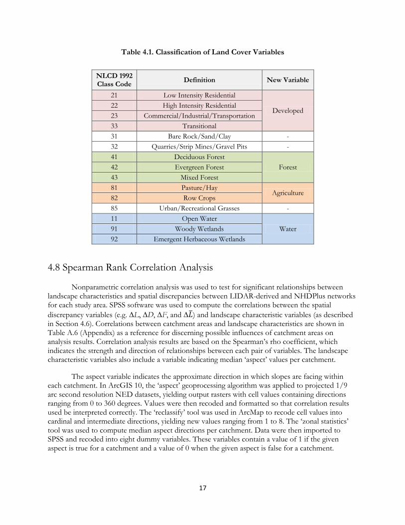
Land cover variables were based on NHDPlus attribute data, which contained percentages of land cover types per catchment derived from the 1992 NLCD (Anderson Level II classification scheme). Relevant NLCD categories were aggregated into the above-mentioned land cover types. The reclassification of NLCD categories is displayed below in Table 4.12.

17

Table 4.1. Classification of Land Cover Variables

NLCD 1992 Class Code

Definition New Variable

21 Low Intensity Residential

Developed 22 High Intensity Residential

23 Commercial/Industrial/Transportation

33 Transitional

31 Bare Rock/Sand/Clay -

32 Quarries/Strip Mines/Gravel Pits -

41 Deciduous Forest

Forest 42 Evergreen Forest

43 Mixed Forest

81 Pasture/Hay Agriculture

82 Row Crops

85 Urban/Recreational Grasses -

11 Open Water

Water 91 Woody Wetlands

92 Emergent Herbaceous Wetlands

4.8 Spearman Rank Correlation Analysis

Nonparametric correlation analysis was used to test for significant relationships between landscape characteristics and spatial discrepancies between LIDAR-derived and NHDPlus networks for each study area. SPSS software was used to compute the correlations between the spatial

discrepancy variables (e.g. ∆L, ∆D, ∆F, and ∆ ) and landscape characteristic variables (as described in Section 4.6). Correlations between catchment areas and landscape characteristics are shown in Table A.6 (Appendix) as a reference for discerning possible influences of catchment areas on analysis results. Correlation analysis results are based on the Spearman’s rho coefficient, which indicates the strength and direction of relationships between each pair of variables. The landscape characteristic variables also include a variable indicating median ‘aspect’ values per catchment.

The aspect variable indicates the approximate direction in which slopes are facing within each catchment. In ArcGIS 10, the ‘aspect’ geoprocessing algorithm was applied to projected 1/9 arc second resolution NED datasets, yielding output rasters with cell values containing directions ranging from 0 to 360 degrees. Values were then recoded and formatted so that correlation results used be interpreted correctly. The ‘reclassify’ tool was used in ArcMap to recode cell values into cardinal and intermediate directions, yielding new values ranging from 1 to 8. The ‘zonal statistics’ tool was used to compute median aspect directions per catchment. Data were then imported to SPSS and recoded into eight dummy variables. These variables contain a value of 1 if the given aspect is true for a catchment and a value of 0 when the given aspect is false for a catchment.

18

Furthermore, positive correlations indicate that as values of a given landscape characteristic variable increase, values of a given spatial discrepancy variable increase. Negative correlations indicate that as values of one variable increase, values of the other variable decrease. For example, a negative correlation between canopy coverage and ∆D would indicate that locally, as canopy coverage per catchment increases, NHDPlus drainage densities become larger than LIDAR-derived drainage densities. On the other hand, a positive correlation between canopy coverage and ∆D would locally show that as canopy coverage increases, LIDAR-derived drainage densities become larger than NHDPlus drainage densities.

19

Chapter 5 Results

5.1 Identifying Reach-Level Spatial Discrepancies

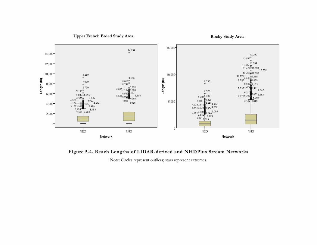
Maps of the networks are displayed in Figures 5.1, 5.2, and 5.3. As shown below in Table 5.1, Mann-Whitney U results indicate that significant differences in reach lengths exist between LIDAR-derived and NHDPlus networks in each of the study areas. Summary statistics (Table A.5 in Appendix) and graphs of network reach length distributions (Figure 5.4) support these results.

Table 5.1. Mann-Whitney U Tests of Reach Length Discrepancies Between LIDAR-derived and NHDPlus Stream Network Datasets

Test UFB ROC PAM

Mann-Whitney U 3,198,127.00 1,519,775.00 1,382,214.00

Wilcoxon W 9,661,937.00 9,295,371.00 2,917,842.00

Z -16.32 -20.35 -2.12

( p-value) 0.00 0.00 0.03

Note: Reach lengths are in meters.

In the Upper French Broad watershed (UFB), the overall spatial composition of LIDAR-derived and NHDPlus networks appear fairly similar, as networks considerably overlap throughout the watershed (Figure 5.1). However, consistently appearing discrepancies between networks are noticeable. According to Figure 5.1, the LIDAR-derived network appears to contain a greater amount of detail than the NHDPlus network in terms of reach frequency, but the lengths of overlapping reaches appear to be consistently shorter in the LIDAR-derived network. The distributions of reaches lengths (Table 5.4) and summary statistics (Table A.1 in Appendix) support these observations.

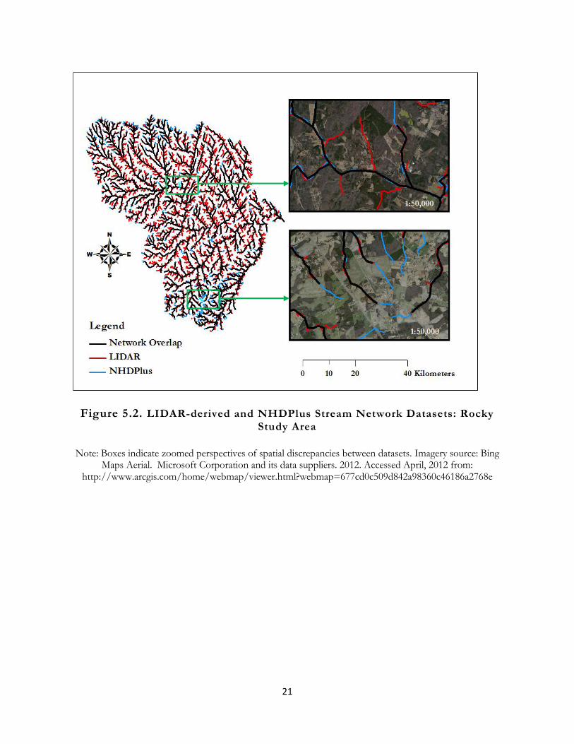
In the Rocky watershed (ROC), stream networks also generally overlap (Figure 5.2). The reach discrepancies look similar to those described of UFB but the differences appear less randomly distributed in ROC study area. In ROC, the LIDAR-derived network contains more than twice as many reaches as NHDPlus and the mean reach length is also approximately twice that of NHDPlus. In addition, the topography and land cover appear more variable in ROC compared to UFB, which may be an indication of the slightly different spatial patterns of discrepancies between the watersheds. According to Figure 5.2, mean reach length discrepancies seem to differ between upper and lower parts of the watershed.

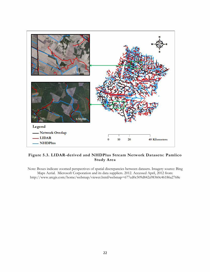
Although LIDAR-derived and NHDPlus networks contain highly similar total numbers of reaches and mean reach lengths in Pamlico watershed (PAM) compared to UFB and ROC study

20

areas, as shown in Figure 5.3, there are clearly substantial differences between the networks throughout PAM. Additional algorithms and techniques commonly need to be used to handle very wide streams or large open waters, divergent streams, and anthropogenic streams such as ditches and canals; all of which are contained within significant portions of PAM study area. Yet, addressing many of these issues is beyond the scope of this study.

Figure 5.1. LIDAR-derived and NHDPlus Stream Network Datasets: Upper French Broad Study Area

Note: Boxes indicate zoomed perspectives of spatial discrepancies between datasets. Imagery source: Bing

Maps Aerial. Microsoft Corporation and its data suppliers. 2012. Accessed April, 2012 from: http://www.arcgis.com/home/webmap/viewer.html?webmap=677cd0c509d842a98360c46186a2768e

21

Figure 5.2. LIDAR-derived and NHDPlus Stream Network Datasets: Rocky

Study Area

Note: Boxes indicate zoomed perspectives of spatial discrepancies between datasets. Imagery source: Bing Maps Aerial. Microsoft Corporation and its data suppliers. 2012. Accessed April, 2012 from:

http://www.arcgis.com/home/webmap/viewer.html?webmap=677cd0c509d842a98360c46186a2768e

22

Figure 5.3. LIDAR-derived and NHDPlus Stream Network Datasets: Pamlico Study Area

Note: Boxes indicate zoomed perspectives of spatial discrepancies between datasets. Imagery source: Bing

Maps Aerial. Microsoft Corporation and its data suppliers. 2012. Accessed April, 2012 from: http://www.arcgis.com/home/webmap/viewer.html?webmap=677cd0c509d842a98360c46186a2768e

Upper French Broad Study Area

Rocky Study Area

Figure 5.4. Reach Lengths of LIDAR-derived and NHDPlus Stream Networks

Note: Circles represent outliers; stars represent extremes.

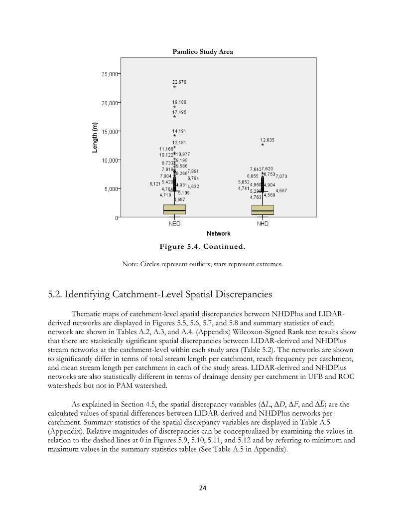
24

Pamlico Study Area

Figure 5.4. Continued.

Note: Circles represent outliers; stars represent extremes.

5.2. Identifying Catchment-Level Spatial Discrepancies

Thematic maps of catchment-level spatial discrepancies between NHDPlus and LIDAR-derived networks are displayed in Figures 5.5, 5.6, 5.7, and 5.8 and summary statistics of each network are shown in Tables A.2, A.3, and A.4. (Appendix) Wilcoxon-Signed Rank test results show that there are statistically significant spatial discrepancies between LIDAR-derived and NHDPlus stream networks at the catchment-level within each study area (Table 5.2). The networks are shown to significantly differ in terms of total stream length per catchment, reach frequency per catchment, and mean stream length per catchment in each of the study areas. LIDAR-derived and NHDPlus networks are also statistically different in terms of drainage density per catchment in UFB and ROC watersheds but not in PAM watershed.

As explained in Section 4.5, the spatial discrepancy variables (∆L, ∆D, ∆F, and ∆ ) are the calculated values of spatial differences between LIDAR-derived and NHDPlus networks per catchment. Summary statistics of the spatial discrepancy variables are displayed in Table A.5 (Appendix). Relative magnitudes of discrepancies can be conceptualized by examining the values in relation to the dashed lines at 0 in Figures 5.9, 5.10, 5.11, and 5.12 and by referring to minimum and maximum values in the summary statistics tables (See Table A.5 in Appendix).

25

In general, interquartile ranges of all spatial discrepancy variables contain both positive and negative values close to 0, and are fairly small compared to upper and lower quartile ranges of the distributions. This infers that overall roughly 50% of catchments contain fairly low differences between networks within each of the study areas. Positive median values of spatial discrepancy variables indicate that a study area contains a higher proportion of catchments containing larger LIDAR-derived values than NHDPlus values for a given spatial discrepancy variable. Negative median values indicate that a given study area contains a higher proportion of catchments containing greater NHDPlus values than LIDAR-derived values for a given variable.

Table 5.2. Wilcoxon-Signed Rank Tests of Catchment-Level Spatial Discrepancies Between LIDAR-derived and NHDPlus Stream Network Datasets

Metric Upper French Broad Rocky Pamlico

Z (p-value)

Z (p-value)

Z (p-value)

L

-2.569 .010

-13.089 .000

-5.174 .000

D

-3.324 .001

-4.157 .000

-0.111 .912

F

-14.804 .000

-16.622 .000

-4.556 .000

-22.902 .000 -19.043 .000 -4.996 .000

Note: Total stream length per catchment (L) measurement units are in m; drainage density per catchment (D) measurement units are in m/ha2; reach frequency per catchment (F) measures N reaches per catchment;

mean reach length per catchment ( ) measurement units are in m. Significant results are boldfaced.

5.2.1 Total Stream Length per Catchment

Distributions of ∆L can be visualized in Figures 5.5 and 5.9. Peak magnitudes of ∆L are much larger in PAM than UFB or ROC sites. In comparison, peak magnitudes of ∆L are less in ROC than PAM and lowest in UFB. The largest magnitudes between networks within each drainage area occur in catchments where the total lengths of LIDAR-derived streams per catchment are greater than the total lengths of NHDPlus streams per catchment. Each study area contains a greater proportion of catchments with longer LIDAR-derived total stream lengths than NHDPlus lengths, respectively. However, this proportional difference is more subtle in UFB.

5.2.2 Drainage Density per Catchment

The spatial distribution of ∆D is illustrated in Figure 5.6. Figure 5.10 and Table A.5 (Appendix) show that the ranges of ∆D are similar between UFB and PAM study areas but the range of ∆D in ROC is considerably less in comparison. As shown by the minimum and maximum values of ∆D in Table A.5 (Appendix), peak magnitudes of ∆D occur in catchments where drainage densities of NHDPlus networks are higher per catchment compared to densities per catchment of LIDAR-derived networks. However, in each study area, there are proportionately more of catchments in which LIDAR-derived networks contain higher drainage densities than NHDPlus networks do (Figure 5.10 and Table A.5 in Appendix).

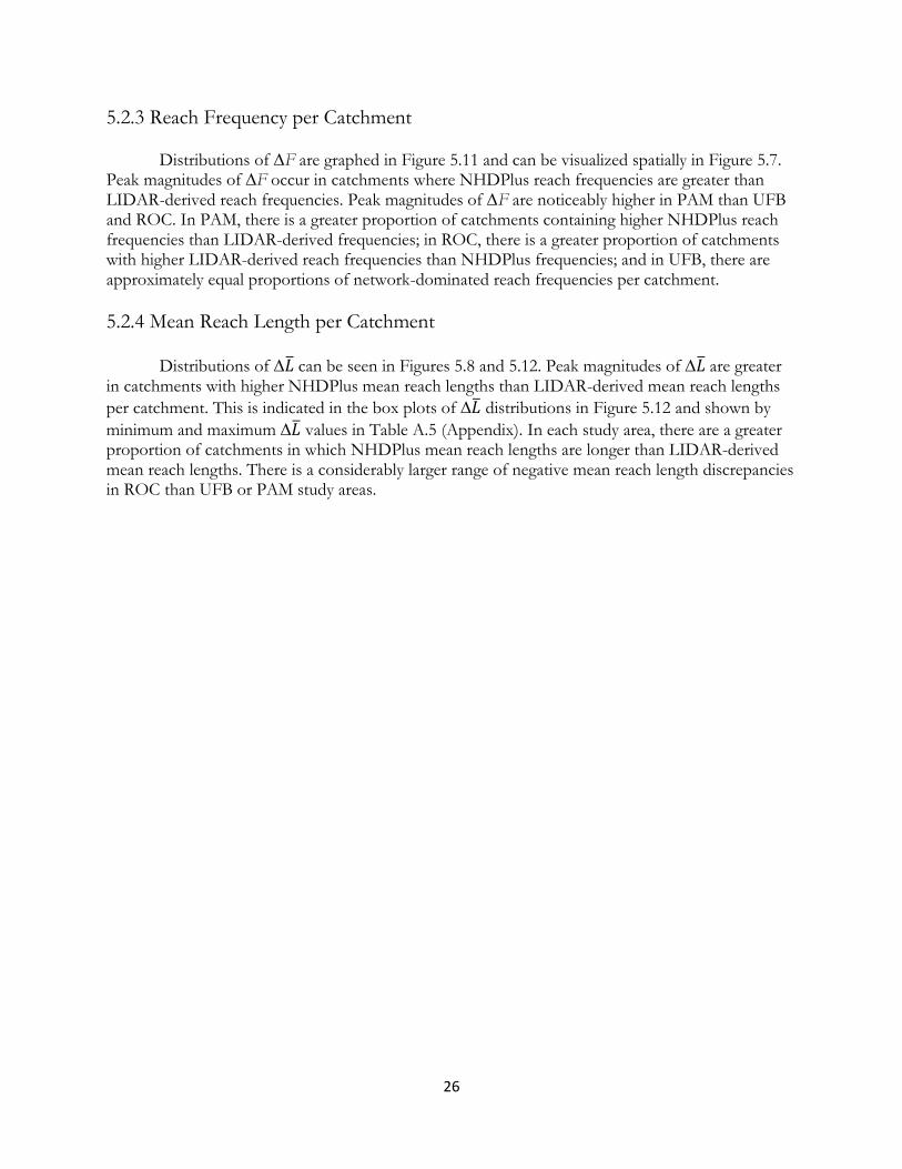
26

5.2.3 Reach Frequency per Catchment

Distributions of ∆F are graphed in Figure 5.11 and can be visualized spatially in Figure 5.7. Peak magnitudes of ∆F occur in catchments where NHDPlus reach frequencies are greater than LIDAR-derived reach frequencies. Peak magnitudes of ∆F are noticeably higher in PAM than UFB and ROC. In PAM, there is a greater proportion of catchments containing higher NHDPlus reach frequencies than LIDAR-derived frequencies; in ROC, there is a greater proportion of catchments with higher LIDAR-derived reach frequencies than NHDPlus frequencies; and in UFB, there are approximately equal proportions of network-dominated reach frequencies per catchment.

5.2.4 Mean Reach Length per Catchment

Distributions of ∆ can be seen in Figures 5.8 and 5.12. Peak magnitudes of ∆ are greater in catchments with higher NHDPlus mean reach lengths than LIDAR-derived mean reach lengths

per catchment. This is indicated in the box plots of ∆ distributions in Figure 5.12 and shown by

minimum and maximum ∆ values in Table A.5 (Appendix). In each study area, there are a greater proportion of catchments in which NHDPlus mean reach lengths are longer than LIDAR-derived mean reach lengths. There is a considerably larger range of negative mean reach length discrepancies in ROC than UFB or PAM study areas.

27

Figure 5.5. Total Stream Length per Catchment Discrepancies between LIDAR -derived and NHDPlus Stream Network Datasets

Note: Values are displayed using septile cut points in ArcMap 10.

28

Figure 5.6. Drainage Density per Catchment Discrepancies between LIDAR -derived and NHDPlus Stream Network Datasets


29

Figure 5.7. Reach Frequency per Catchment Discrepancies between LIDAR -derived and NHDPlus Stream Network Datasets


30

Figure 5.8. Mean Reach Length per Catchment Discrepancies between LIDAR -derived and NHDPlus Stream Network Datasets


31

Figure 5.9. Discrepancies in Total Stream Length Per Catchment Between LIDAR-derived and NHDPlus Datasets: Upper French Broad, Rocky, and

Pamlico Drainage Areas Note: Values represent the magnitude of differences in total stream length per catchment between LIDAR-derived and NHDPlus networks for each study area. Discrepancy values can be conceptualized as follows:

(Total LIDAR-derived stream length per catchment) – (Total NHDPlus stream length per catchment)

Values above the dashed line indicate where total LIDAR-derived stream length per catchment > total NHDPlus stream length per catchment. Values below the dashed line denote where total NHDPlus stream length per catchment > total LIDAR-derived frequency per catchment. Circles represent outliers; stars represent extremes.

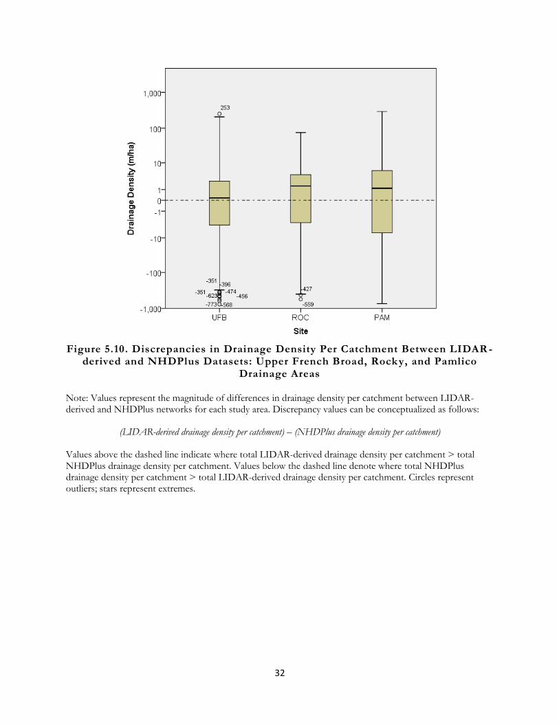
32

Figure 5.10. Discrepancies in Drainage Density Per Catchment Between LIDAR -

derived and NHDPlus Datasets: Upper French Broad, Rocky, and Pamlico Drainage Areas

Note: Values represent the magnitude of differences in drainage density per catchment between LIDAR-derived and NHDPlus networks for each study area. Discrepancy values can be conceptualized as follows:

(LIDAR-derived drainage density per catchment) – (NHDPlus drainage density per catchment)

Values above the dashed line indicate where total LIDAR-derived drainage density per catchment > total NHDPlus drainage density per catchment. Values below the dashed line denote where total NHDPlus drainage density per catchment > total LIDAR-derived drainage density per catchment. Circles represent outliers; stars represent extremes.

33

Figure 5.11. Discrepancies in Reach Frequency Per Catchment Between LIDAR -

derived and NHDPlus Datasets: Upper French Broad, Rocky, and Pamlico Drainage Areas

Note: Values represent the magnitude of differences in reach frequency per catchment between LIDAR-derived and NHDPlus networks for each study area. Discrepancy values can be conceptualized as follows:

(LIDAR-derived reach frequency per catchment) – (NHDPlus reach frequency per catchment)

Values above the dashed line indicate where total LIDAR-derived reach frequency per catchment > total NHDPlus frequency per catchment. Values below the dashed line denote where total NHDPlus reach frequency per catchment > total LIDAR-derived frequency per catchment. Circles represent outliers; stars represent extremes.

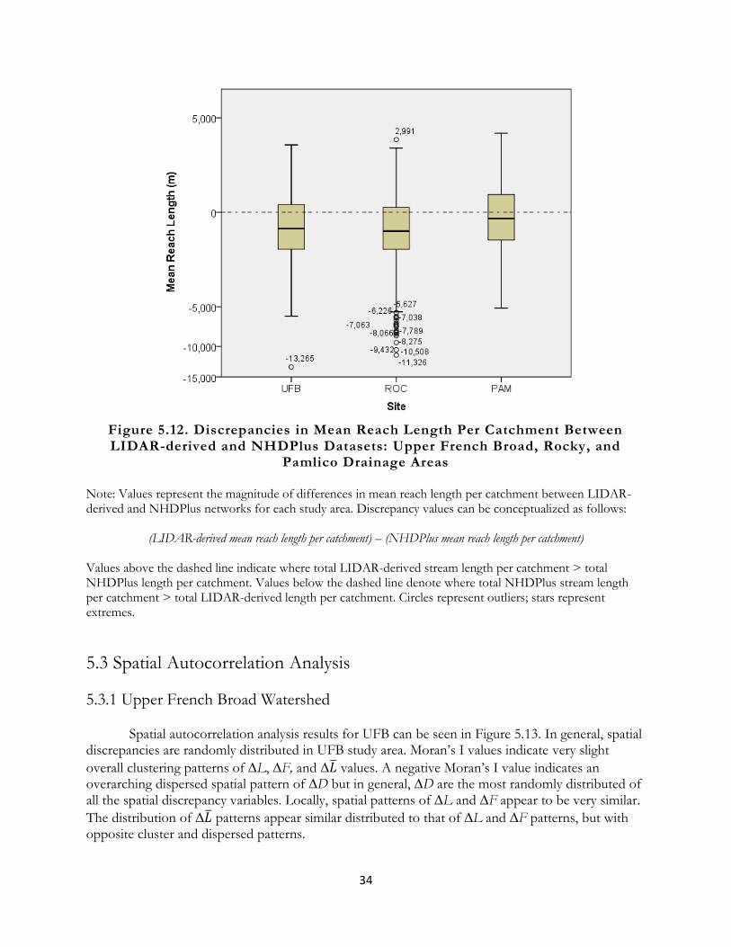
34

Figure 5.12. Discrepancies in Mean Reach Length Per Catchment Between LIDAR-derived and NHDPlus Datasets: Upper French Broad, Rocky, and

Pamlico Drainage Areas Note: Values represent the magnitude of differences in mean reach length per catchment between LIDAR-derived and NHDPlus networks for each study area. Discrepancy values can be conceptualized as follows:

(LIDAR-derived mean reach length per catchment) – (NHDPlus mean reach length per catchment)

Values above the dashed line indicate where total LIDAR-derived stream length per catchment > total NHDPlus length per catchment. Values below the dashed line denote where total NHDPlus stream length per catchment > total LIDAR-derived length per catchment. Circles represent outliers; stars represent extremes.

5.3 Spatial Autocorrelation Analysis

5.3.1 Upper French Broad Watershed

Spatial autocorrelation analysis results for UFB can be seen in Figure 5.13. In general, spatial discrepancies are randomly distributed in UFB study area. Moran’s I values indicate very slight

overall clustering patterns of ∆L, ∆F, and ∆ values. A negative Moran’s I value indicates an overarching dispersed spatial pattern of ∆D but in general, ∆D are the most randomly distributed of all the spatial discrepancy variables. Locally, spatial patterns of ∆L and ∆F appear to be very similar.

The distribution of ∆ patterns appear similar distributed to that of ∆L and ∆F patterns, but with opposite cluster and dispersed patterns.

35

5.3.2 Rocky Watershed

Spatial autocorrelation analysis results for ROC study area are displayed in Figure 5.14. Spatial patterns and corresponding Moran’s I values show that significant local patterns are much more prevalent throughout ROC in comparison to UFB; yet, dominant spatial patterns of individual metrics appear similar between the two study areas. Like UFB study area, significant local ∆L and

∆F are similarly distributed and ∆ patterns appear similarly distributed to ∆L and ∆F patterns but with opposite cluster and dispersed patterns. Like UFB study area, ∆D are also the most randomly distributed of all the spatial discrepancy variables in ROC.

Although ∆D cluster and dispersed patterns are not substantially prevalent within ROC, the

watershed scale pattern is slightly more clustered than dispersed (Moran’s I = 0.017) and contains predominantly high-high clusters. Further, a large proportion of the high-high ∆D clusters appear to agglomerate heavily along the main channel within ROC.

5.3.3 Pamlico Watershed

As indicated in Figure 5.15 by the positive Moran’s I values and relative proportions and distributions of spatial patterns, clustering patterns are generally more prominent to varying degrees than dispersed patterns for each type of spatial discrepancy within PAM study area. In contrast to UFB and ROC study areas, ∆L and ∆F patterns do not appear markedly similar to each other. High-high ∆L clusters tend to be comprised of relatively large catchments, which are primarily agglomerated across the northern part of the watershed. Respectively, low-low ∆L clusters are mainly located within a few scattered groups of relatively small catchments. Proportions and distributions of ∆F pattern types highly vary within PAM; a prominent arrangement of high-high ∆F values coalesce in a sinuous fashion from the northeastern to the western middle portion of the watershed. At the watershed scale, Moran’s I values indicate that overall clustering of ∆L and ∆F are generally stronger overall in ROC and PAM than in UFB study area.

The Moran’s I value indicates that ∆ values are randomly distributed overall. Similar to UFB and PAM, there are relatively few statistically significant local ∆D patterns; ∆D values are primarily randomly distributed throughout the watershed as indicated by the Moran’s I value (0.071). Significant local ∆D patterns are mainly of high-high clusters.

36

Figure 5.13. Spatial Autocorrelation Analysis of Spatial Discrepancies between

LIDAR-derived and NHDPlus Stream Networks in Upper French Broad Drainage Area

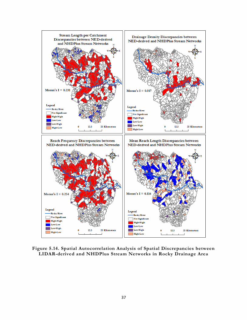
37

Figure 5.14. Spatial Autocorrelation Analysis of Spatial Discrepancies between LIDAR-derived and NHDPlus Stream Networks in Rocky Drainage Area

38

Figure 5.15. Spatial Autocorrelation Analysis of Spatial Discrepancies between LIDAR-derived and NHDPlus Stream Networks in Pamlico Drainage Area

39

5.4 Spatial Discrepancy Patterns and Landscape Characteristics

Results of Kruskal-Wallis tests are shown in Tables 5.3, 5.4, 5.5 and 5.6 and distributions of landscape characteristic variables are displayed in Figures 5.16 through 5.222. Results show that several individual landscape characteristics significantly differ between spatial discrepancy pattern groups within the study areas. Median values indicate relative differences of landscape variables between groups within and between study areas. Many analyses contain groups with unequal sample sizes, which may potentially influence results of some significance tests. Taking into account the differences in sample sizes and median values of significant results, some overarching associations can be discerned.

5.4.1 Total Stream Length Discrepancy Patterns

Kruskal-Wallis test results in terms of ∆L patterns are shown in Table 5.3. Results indicate that larger catchments generally tend toward clusters containing longer total lengths of LIDAR-derived streams than NHDPlus streams in each of the study areas (high-high group).

In UFB, lower percentages of canopy coverage are more associated with longer total lengths

of LIDAR-derived streams than NHDPlus streams (high-high group) whereas higher percentages of canopy coverage are more associated with longer total lengths of NHDPlus streams than LIDAR-derived streams (low-low group). In ROC, percentages of canopy coverage in the “low-low” group are significantly lower than the other groups. There are significant differences in mean slope between groups as well for each study area.

In PAM study area, there is a significantly greater proportion of forest land per catchment in

the low-low group than the other groups. There are also significant differences in proportions of agricultural land and water between groups in UFB and PAM. In UFB, considerably greater proportions of water per catchment tend toward the high-high group compared to the other groups. In ROC, substantially greater proportions of water per catchment tend toward the high-high group compared to other groups, especially the low-low group. Significant differences in proportions of water per catchment also exist in PAM study area.

5.4.2 Drainage Density Discrepancy Patterns

Results of Kruskal-Wallis tests in terms of ∆D patterns are displayed in Table 5.4.

Associations between ∆D patterns and catchment areas are similar within each of the study areas, in which clusters of catchments containing higher LIDAR-derived drainage densities compared to NHDPlus densities (high-high group) are generally within larger catchments compared to the other groups. In UFB and ROC, proportions of canopy coverage tend to be significantly higher in the high-high than low-low cluster groups. Slope also significantly differs between groups in ROC and PAM. In PAM, results show that steeper slopes are more associated with high-high ∆D clusters than other local patterns.

2 Aspect is not a variable included in the Kruskal Wallis tests. Relationships between aspect and spatial discrepancies between the NHDPlus and LIDAR-derived networks are discussed in the Spearman Rank Correlation analysis results (Section 5.5).

40

Regarding land cover variables, all of the developed land is within high-low catchments in ROC study area. There are also significant differences in proportions of forest land and water between certain groups in ROC and PAM. Significant differences in proportions of agricultural land also exist between groups within UFB and PAM.

5.4.3 Reach Frequency Discrepancy Patterns

Kruskal-Wallis analysis findings regarding ∆F patterns are shown in Table 5.5. Catchment areas generally tend to be significantly larger in high-high clusters than the other groups for ROC and PAM study areas. There are also significant differences in percentages of canopy coverage between groups for UFB and PAM study areas.

In terms of land cover, proportions of forest land in PAM study area are significantly higher within high-high clusters, especially compared to low-low clusters. Significant differences also exist between groups with agricultural land and water in ROC and agricultural land in UFB.

5.4.4 Mean Reach Length Discrepancy Patterns

Results of Kruskal-Wallis tests in terms of ∆ patterns are presented in Table 5.6. Catchment areas tend to be considerably smaller within high-high clusters than catchment areas within low-low clusters in ROC and PAM. There are also significant differences between percentages of canopy coverage between groups within UFB and PAM. In PAM, percentages of canopy coverage are considerably lower in high-high clusters than low-low clusters. Considering the land cover variables, there are significantly greater proportions of developed land within the low-high group than other groups in UFB. In ROC, there are significantly greater proportions of developed land within high-high clusters than the other groups, especially than the high-low group. Proportions of agricultural land and land cover type water also significantly differ between groups within ROC and PAM study areas.

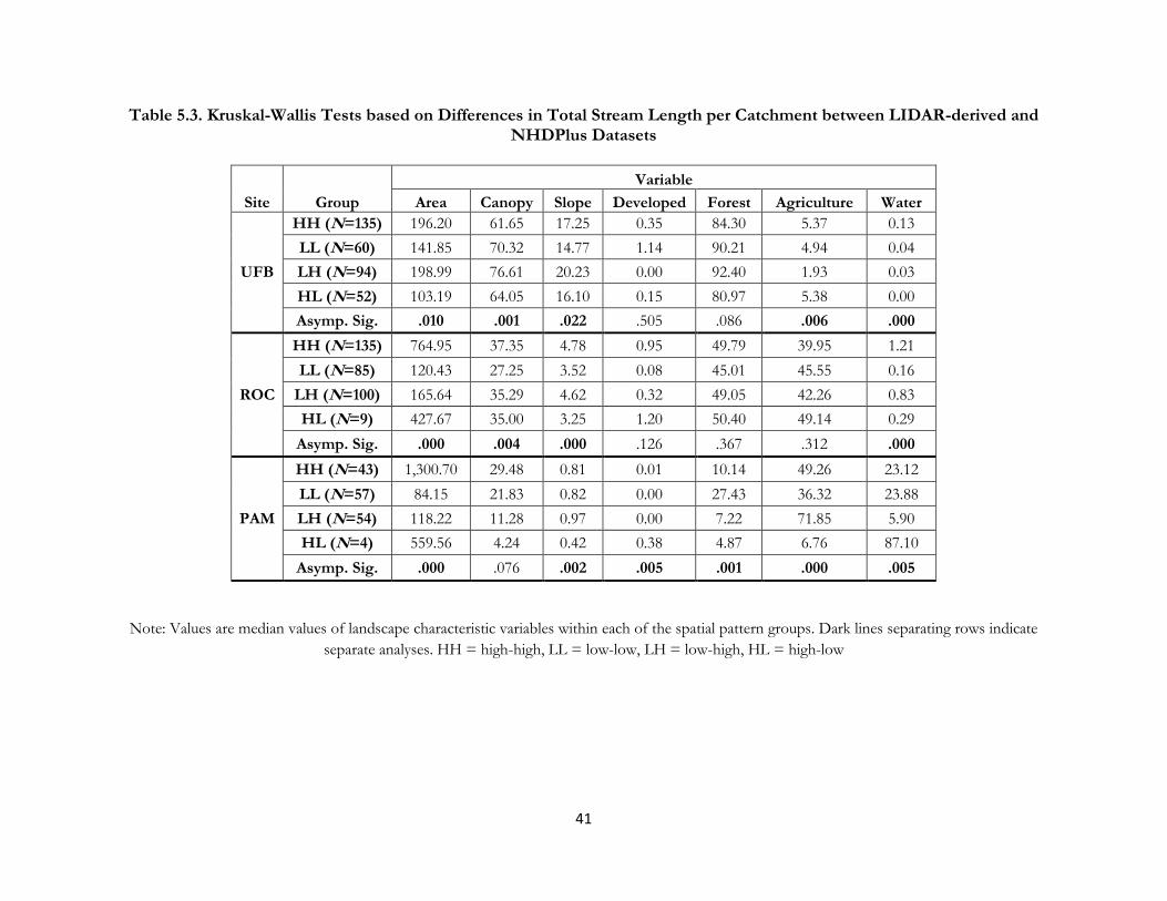
41

Table 5.3. Kruskal-Wallis Tests based on Differences in Total Stream Length per Catchment between LIDAR-derived and NHDPlus Datasets

Site Group

Variable

Area Canopy Slope Developed Forest Agriculture Water

UFB

HH (N=135) 196.20 61.65 17.25 0.35 84.30 5.37 0.13

LL (N=60) 141.85 70.32 14.77 1.14 90.21 4.94 0.04

LH (N=94) 198.99 76.61 20.23 0.00 92.40 1.93 0.03

HL (N=52) 103.19 64.05 16.10 0.15 80.97 5.38 0.00

Asymp. Sig. .010 .001 .022 .505 .086 .006 .000

ROC

HH (N=135) 764.95 37.35 4.78 0.95 49.79 39.95 1.21

LL (N=85) 120.43 27.25 3.52 0.08 45.01 45.55 0.16

LH (N=100) 165.64 35.29 4.62 0.32 49.05 42.26 0.83

HL (N=9) 427.67 35.00 3.25 1.20 50.40 49.14 0.29

Asymp. Sig. .000 .004 .000 .126 .367 .312 .000

PAM

HH (N=43) 1,300.70 29.48 0.81 0.01 10.14 49.26 23.12

LL (N=57) 84.15 21.83 0.82 0.00 27.43 36.32 23.88

LH (N=54) 118.22 11.28 0.97 0.00 7.22 71.85 5.90

HL (N=4) 559.56 4.24 0.42 0.38 4.87 6.76 87.10

Asymp. Sig. .000 .076 .002 .005 .001 .000 .005

Note: Values are median values of landscape characteristic variables within each of the spatial pattern groups. Dark lines separating rows indicate

separate analyses. HH = high-high, LL = low-low, LH = low-high, HL = high-low

42

Table 5.4. Kruskal-Wallis Tests based on Differences in Drainage Density per Catchment between LIDAR-derived and NHDPlus Datasets

Site Group

Variable


UFB

HH (N=66) 139.28 57.54 14.74 0.15 75.60 4.44 0.30

LL (N=12) 32.04 53.18 10.91 0.00 77.30 9.66 0.54

LH (N=14) 63.22 71.81 12.91 2.10 80.37 0.16 0.10

HL (N=35) 66.96 52.85 9.60 2.62 69.23 12.89 0.46

Asymp. Sig. .002 .705 .056 .342 .606 .002 .936

ROC

HH (N=82) 317.61 36.94 5.36 0.00 53.39 39.74 1.84

LL (N=13) 16.20 13.32 4.07 0.00 41.38 50.00 1.67

LH (N=6) 65.88 20.16 2.86 0.00 46.51 51.38 0.00

HL (N=21) 53.53 31.62 5.00 4.93 47.32 36.96 0.21

Asymp. Sig. .000 .001 .000 .001 .047 .113 .001

PAM

HH (N=66) 92.07 34.65 1.01 0.00 36.90 10.67 40.82

LL (N=12) 12.06 0.00 0.78 0.00 0.00 0.00 100.00

LH (N=14) 6.03 12.73 0.79 0.00 9.19 0.81 79.14

HL (N=35) 92.12 16.29 0.82 0.00 15.47 7.62 62.79

Asymp. Sig. .002 .000 .003 .115 .000 .038 .001



43

Table 5.5. Kruskal-Wallis Tests based on Differences in Reach Frequency per Catchment between LIDAR-derived and NHDPlus Datasets

Site Group

Variable


UFB

HH (N=125) 139.93 77.41 17.53 0.00 94.55 1.79 0.00

LL (N=77) 156.60 73.69 18.27 0.00 90.68 5.36 0.06

LH (N=119) 114.74 66.16 16.26 0.00 87.82 2.70 0.01

HL (N=43) 185.93 68.18 15.13 0.18 91.29 4.71 0.11

Asymp. Sig. .077 .042 .607 .812 .165 .027 .068

ROC

HH (N=143) 726.93 38.32 4.72 0.94 50.67 39.45 1.27

LL (N=70) 51.80 36.17 4.36 0.00 53.69 28.01 0.15

LH (N=105) 187.74 36.81 4.60 0.17 48.71 40.87 0.61

HL (N=17) 263.33 38.00 4.58 3.25 52.74 34.90 0.37

Asymp. Sig. .000 .741 .362 .075 .716 .003 .000

PAM

HH (N=125) 440.10 35.39 0.97 0.02 33.55 22.65 26.70

LL (N=77) 99.89 9.65 0.84 0.00 7.19 45.55 14.01

LH (N=119) 143.99 18.35 0.87 0.00 12.46 32.40 32.53

HL (N=43) 208.57 23.67 0.83 0.00 14.24 36.65 31.07

Asymp. Sig. .000 .000 .058 .006 .000 .149 .106

Note: Values are median values of landscape characteristic variables within each of the spatial pattern groups. Dark lines separating rows

indicate separate analyses. HH = high-high, LL = low-low, LH = low-high, HL = high-low

44

Table 5.6. Kruskal-Wallis Tests based on Differences in Mean Reach Length per Catchment between LIDAR-derived and NHDPlus Datasets

Site Group

Variable


UFB

HH (N=87) 156.60 72.13 15.22 0.49 88.74 4.09 0.06

LL (N=95) 127.90 75.58 17.53 0.00 93.30 2.16 0.00

LH (N=33) 137.43 58.75 14.41 7.25 78.55 3.27 0.06

HL (N=119) 117.81 82.12 17.38 0.00 94.53 1.51 0.00

Asymp. Sig. .500 .036 .339 .000 .029 .203 .575

ROC

HH (N=93) 73.44 35.48 4.64 4.19 51.15 21.02 0.32

LL (N=74) 781.53 32.63 4.33 1.54 45.57 41.34 1.05

LH (N=11) 140.48 39.08 4.20 0.17 57.89 28.95 0.10

HL (N=95) 242.48 36.11 4.62 0.09 48.21 42.23 0.93

Asymp. Sig. .000 .616 .302 .001 .352 .000 .001

PAM

HH (N=87) 57.55 19.13 0.85 0.00 18.04 5.20 56.48

LL (N=95) 297.00 35.32 0.88 0.04 30.36 26.82 17.41

LH (N=33) 160.57 22.04 0.88 0.00 17.25 5.31 46.30

HL (N=119) 93.68 24.95 1.01 0.00 30.46 13.02 38.44

Asymp. Sig. .000 .029 .499 .295 .028 .046 .001



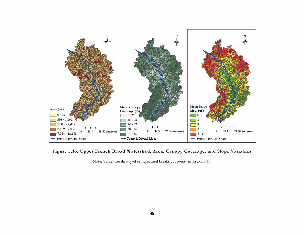
45

Figure 5.16. Upper French Broad Watershed: Area, Canopy Coverage, and Slope Variables

Note: Values are displayed using natural breaks cut points in ArcMap 10.

46

Figure 5.17. Rocky Watershed: Area, Canopy Coverage, and Slope Variables


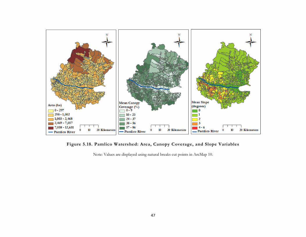
47

Figure 5.18. Pamlico Watershed: Area, Canopy Coverage, and Slope Variables


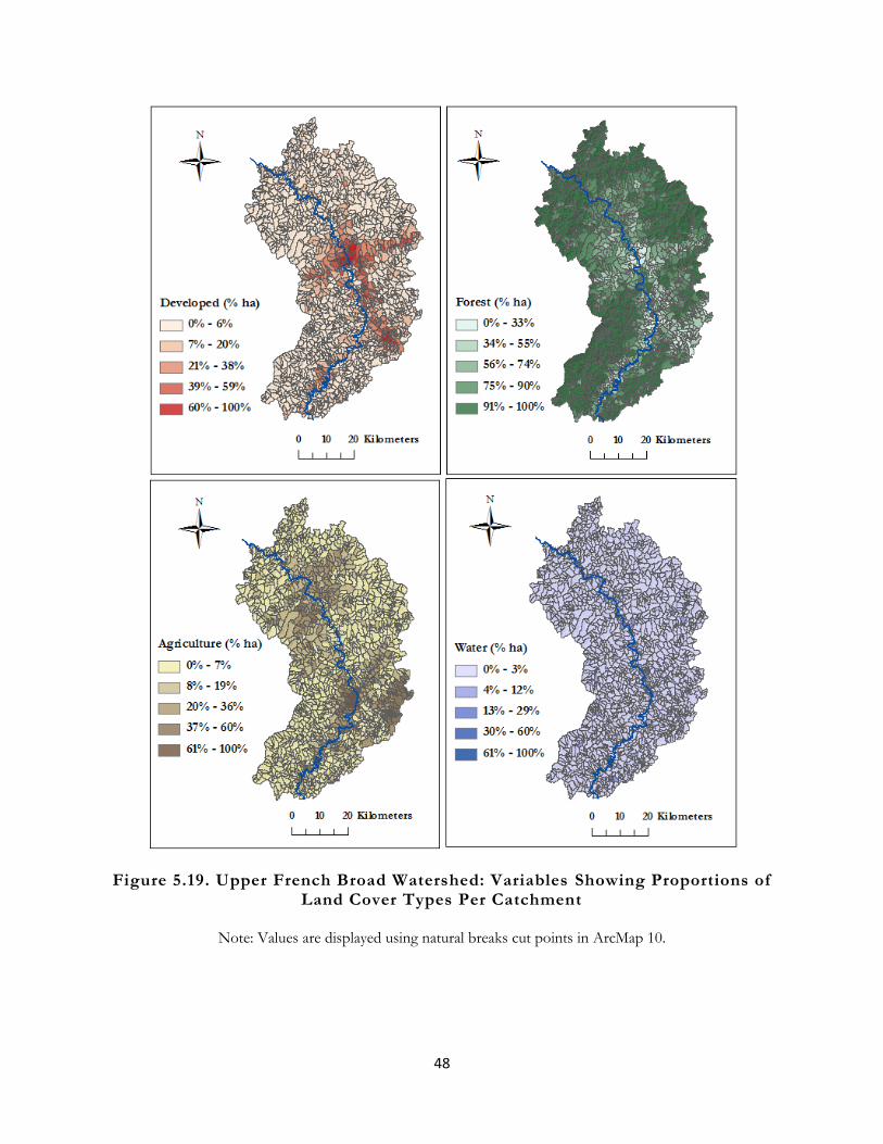
48

Figure 5.19. Upper French Broad Watershed: Variables Showing Proportions of Land Cover Types Per Catchment


49

Figure 5.20. Rocky Watershed: Variables Showing Proportions of Land Cover Types Per Catchment


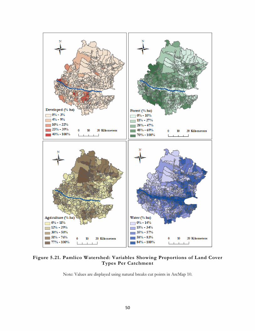
50

Figure 5.21. Pamlico Watershed: Variables Showing Proportions of Land Cover Types Per Catchment


51

Figure 5.22. Aspect per Catchment: Upper French Broad, Rocky, and Pamlico Watersheds

52

5.5 Spearman Rank Correlation Analysis Results

Spearman Rank Correlation test results show that there are several significant correlations between landscape characteristics (Figures 5.16 through 5.22) and spatial discrepancies between the LIDAR-derived and NHDPlus stream networks in each of the study areas. Significant correlations between landscape characteristics and catchment areas additionally indicate that catchment area may be a factor influencing some relationships between landscape characteristic variables and spatial discrepancy variables (See Table A.6 in Appendix).

5.5.1 Total Stream Length per Catchment

Correlation analysis results between ∆L and landscape variables are displayed in Table 5.7. A strong positive correlation exists between ∆L and catchment area in ROC (Rho = 0.685, Sig. =0 .000). A slightly strong relationship between ∆L and catchment area also exists in PAM (Rho = 0.361, 0.000) and a lower significant relationship exists in UFB. Relationships are also significant between ∆L and canopy coverage, and ∆L and slope, in each of the study areas. ∆L are negatively related to percent canopy coverage in UFB, and positively related to canopy coverage in ROC and PAM. A negative correlation exists between slope and ∆L in UFB, and positive relationships exist between slope and ∆L in ROC and PAM study areas.

Results also show that ∆L are significantly related to various land cover variables. Positive

relationships exist in each study area between ∆L and developed land. ∆L are negatively related to forest in UFB and positively related to forest in ROC and PAM. ∆L is positively related to agriculture in UFB. Water is positively related to ∆L values in each of the study areas but more strongly in ROC study area (Rho = 0.337, Sig. = 0.000).

Low correlations exist between ∆L and specific aspects. In UFB, ∆L are negatively

correlated with south-facing slopes and positively related to northwest-facing slopes. A slight positive relationship also exists between ∆L and northern aspects in UFB. ∆L values are positively related to east-facing slopes and negatively related to south-facing slopes in ROC. PAM study area contains slightly significant positive relationships between ∆L and northeast aspects and ∆L and southwest aspects.

5.5.2 Drainage Density per Catchment

Correlation analysis results between ∆D values and landscape variables are displayed in Table 5.8. The strongest relationship is between ∆D and catchment area in ROC watershed (Rho = 0.510, Sig. = 0.000). A slightly strong relationship between ∆D and catchment area also exists within PAM (Rho = 0.227, Sig. = 0.000). Significant correlations exist for each of the study areas between ∆D and canopy coverage, and ∆D and slope. A slightly strong relationship exists between ∆D and slope in ROC (Rho =0.228, Sig. = 0.000). Slope and canopy coverage are each negatively related to ∆D in UFB and positively related to ∆D in ROC and PAM.

Several correlations exist between ∆D and types of land cover. ∆D is positively related to

both developed land and water in each of the study areas. Forest and ∆D are negatively related in UFB and positively correlated in ROC and PAM. There is a weak positive relationship between ∆D

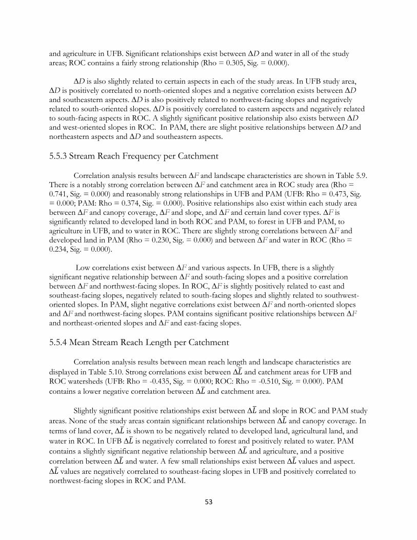
53

and agriculture in UFB. Significant relationships exist between ∆D and water in all of the study areas; ROC contains a fairly strong relationship (Rho = 0.305, Sig. = 0.000).

∆D is also slightly related to certain aspects in each of the study areas. In UFB study area,

∆D is positively correlated to north-oriented slopes and a negative correlation exists between ∆D and southeastern aspects. ∆D is also positively related to northwest-facing slopes and negatively related to south-oriented slopes. ∆D is positively correlated to eastern aspects and negatively related to south-facing aspects in ROC. A slightly significant positive relationship also exists between ∆D and west-oriented slopes in ROC. In PAM, there are slight positive relationships between ∆D and northeastern aspects and ∆D and southeastern aspects.

5.5.3 Stream Reach Frequency per Catchment

Correlation analysis results between ∆F and landscape characteristics are shown in Table 5.9. There is a notably strong correlation between ∆F and catchment area in ROC study area (Rho = 0.741, Sig. = 0.000) and reasonably strong relationships in UFB and PAM (UFB: Rho = 0.473, Sig. = 0.000; PAM: Rho = 0.374, Sig. = 0.000). Positive relationships also exist within each study area between ∆F and canopy coverage, ∆F and slope, and ∆F and certain land cover types. ∆F is significantly related to developed land in both ROC and PAM, to forest in UFB and PAM, to agriculture in UFB, and to water in ROC. There are slightly strong correlations between ∆F and developed land in PAM (Rho = 0.230, Sig. = 0.000) and between ∆F and water in ROC (Rho = 0.234, Sig. = 0.000).

Low correlations exist between ∆F and various aspects. In UFB, there is a slightly

significant negative relationship between ∆F and south-facing slopes and a positive correlation between ∆F and northwest-facing slopes. In ROC, ∆F is slightly positively related to east and southeast-facing slopes, negatively related to south-facing slopes and slightly related to southwest-oriented slopes. In PAM, slight negative correlations exist between ∆F and north-oriented slopes and ∆F and northwest-facing slopes. PAM contains significant positive relationships between ∆F and northeast-oriented slopes and ∆F and east-facing slopes.

5.5.4 Mean Stream Reach Length per Catchment

Correlation analysis results between mean reach length and landscape characteristics are

displayed in Table 5.10. Strong correlations exist between ∆ and catchment areas for UFB and ROC watersheds (UFB: Rho = -0.435, Sig. = 0.000; ROC: Rho = -0.510, Sig. = 0.000). PAM

contains a lower negative correlation between ∆ and catchment area.

Slightly significant positive relationships exist between ∆ and slope in ROC and PAM study

areas. None of the study areas contain significant relationships between ∆ and canopy coverage. In

terms of land cover, ∆ is shown to be negatively related to developed land, agricultural land, and

water in ROC. In UFB ∆ is negatively correlated to forest and positively related to water. PAM

contains a slightly significant negative relationship between ∆ and agriculture, and a positive

correlation between ∆ and water. A few small relationships exist between ∆ values and aspect.

∆ values are negatively correlated to southeast-facing slopes in UFB and positively correlated to northwest-facing slopes in ROC and PAM.

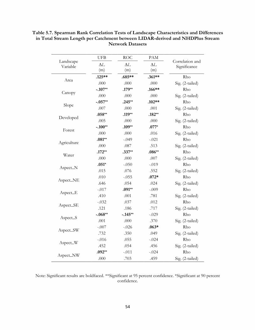
54

Table 5.7. Spearman Rank Correlation Tests of Landscape Characteristics and Differences in Total Stream Length per Catchment between LIDAR-derived and NHDPlus Stream

Network Datasets

Landscape Variable

UFB

ROC

PAM

Correlation and Significance ∆L

(m) ∆L

(m) ∆L

(m)

Area .125** .685** .361** Rho

.000 .000 .000 Sig. (2-tailed)

Canopy -.107**

.179**

.166**

Rho

.000

.000

.000

Sig. (2-tailed)

Slope -.057**

.245**

.102**

Rho

.007

.000

.001

Sig. (2-tailed)

Developed .058**

.119**

.182**

Rho

.005

.000

.000

Sig. (2-tailed)

Forest -.100**

.109**

.077*

Rho

.000

.000

.016

Sig. (2-tailed)

Agriculture .081**

-.049

-.021

Rho

.000

.087

.513

Sig. (2-tailed)

Water .172**

.337**

.086**

Rho

.000

.000

.007

Sig. (2-tailed)

Aspect_N .051*

-.050

-.019

Rho

.015

.076

.552

Sig. (2-tailed)

Aspect_NE .010

-.055

.072*

Rho

.646

.054

.024

Sig. (2-tailed)

Aspect_E -.017

.091**

-.009

Rho

.410

.001

.781

Sig. (2-tailed)

Aspect_SE -.032

.037

.012

Rho

.121

.186

.717

Sig. (2-tailed)

Aspect_S -.068**

-.145**

-.029

Rho

.001

.000

.370

Sig. (2-tailed)

Aspect_SW -.007

-.026

.063*

Rho

.732

.350

.049

Sig. (2-tailed)

Aspect_W -.016

.055

-.024

Rho

.452

.054

.456

Sig. (2-tailed)

Aspect_NW .092**

-.011

-.024

Rho

.000

.703

.459

Sig. (2-tailed)

Note: Significant results are boldfaced. **Significant at 95 percent confidence. *Significant at 90 percent confidence.

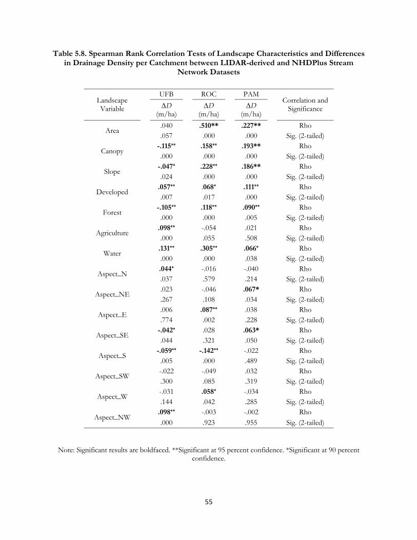
55

Table 5.8. Spearman Rank Correlation Tests of Landscape Characteristics and Differences in Drainage Density per Catchment between LIDAR-derived and NHDPlus Stream

Network Datasets

Landscape Variable

UFB

ROC

PAM

Correlation and Significance

∆D

(m/ha) ∆D

(m/ha) ∆D

(m/ha)

Area .040 .510** .227** Rho

.057 .000 .000 Sig. (2-tailed)

Canopy -.115**

.158**

.193**

Rho

.000

.000

.000

Sig. (2-tailed)

Slope -.047*

.228**

.186**

Rho

.024

.000

.000

Sig. (2-tailed)

Developed .057**

.068*

.111**

Rho

.007

.017

.000

Sig. (2-tailed)

Forest -.105**

.118**

.090**

Rho

.000

.000

.005

Sig. (2-tailed)

Agriculture .098**

-.054

.021

Rho

.000

.055

.508

Sig. (2-tailed)

Water .131**

.305**

.066*

Rho

.000

.000

.038

Sig. (2-tailed)

Aspect_N .044*

-.016

-.040

Rho

.037

.579

.214

Sig. (2-tailed)

Aspect_NE .023

-.046

.067*

Rho

.267

.108

.034

Sig. (2-tailed)

Aspect_E .006

.087**

.038

Rho

.774

.002

.228

Sig. (2-tailed)

Aspect_SE -.042*

.028

.063*

Rho

.044

.321

.050

Sig. (2-tailed)

Aspect_S -.059**

-.142**

-.022

Rho

.005

.000

.489

Sig. (2-tailed)

Aspect_SW -.022

-.049

.032

Rho

.300

.085

.319

Sig. (2-tailed)

Aspect_W -.031

.058*

-.034

Rho

.144

.042

.285

Sig. (2-tailed)

Aspect_NW .098**

-.003

-.002

Rho

.000

.923

.955

Sig. (2-tailed)

Note: Significant results are boldfaced. **Significant at 95 percent confidence. *Significant at 90 percent

confidence.

56

Table 5.9. Spearman Rank Correlation Analysis of Landscape Characteristics and Differences in Reach Frequency per Catchment between LIDAR-derived and NHDPlus

Stream Network Datasets

Landscape Variable

UFB

ROC

PAM


∆F

(N reaches) ∆F

(N reaches) ∆F

(N reaches)

Area .473** .741** .374** Rho

.000 .000 .000 Sig. (2-tailed)

Canopy .070**

.094**

.198**

Rho

.001

.001

.000

Sig. (2-tailed)

Slope .151**

.125**

.123**

Rho

.000

.000

.000

Sig. (2-tailed)

Developed .016

.122**

.230**

Rho

.448

.000

.000

Sig. (2-tailed)

Forest .057**

.042

.199**

Rho

.007

.140

.000

Sig. (2-tailed)

Agriculture .042*

.046

.018

Rho

.047

.104

.574

Sig. (2-tailed)

Water -.038

.234**

.001

Rho

.073

.000

.972

Sig. (2-tailed)

Aspect_N .017

-.027

-.064*

Rho

.409

.349

.045

Sig. (2-tailed)

Aspect_NE -.009

-.046

.099**

Rho

.654

.108

.002

Sig. (2-tailed)

Aspect_E .024

.059*

.067*

Rho

.255

.036

.035

Sig. (2-tailed)

Aspect_SE .011

.061*

-.022

Rho

.590

.031

.487

Sig. (2-tailed)

Aspect_S -.051*

-.128**

.014

Rho

.015

.000

.662

Sig. (2-tailed)

Aspect_SW -.030

-.066*

.038

Rho

.157

.021

.232

Sig. (2-tailed)

Aspect_W -.017

.044

-.026

Rho

.423

.118

.415

Sig. (2-tailed)

Aspect_NW .058**

.026

-.077*

Rho

.005

.353

.016

Sig. (2-tailed)

Note: Significant results are boldfaced. **Significant at 95 percent confidence. *Significant at 90 percent

confidence.

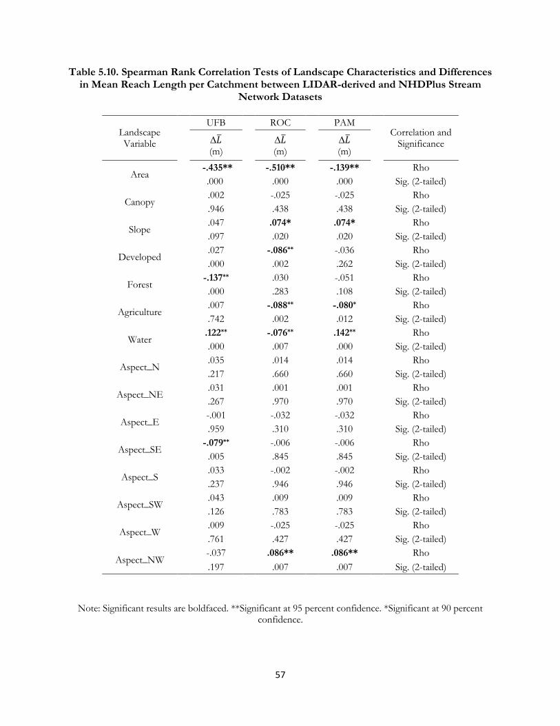
57

Table 5.10. Spearman Rank Correlation Tests of Landscape Characteristics and Differences in Mean Reach Length per Catchment between LIDAR-derived and NHDPlus Stream

Network Datasets

Landscape Variable

UFB

ROC

PAM


∆

(m) ∆

(m) ∆

(m)

Area -.435** -.510** -.139** Rho

.000 .000 .000 Sig. (2-tailed)

Canopy .002

-.025

-.025

Rho

.946

.438

.438

Sig. (2-tailed)

Slope .047

.074*

.074*

Rho

.097

.020

.020

Sig. (2-tailed)

Developed .027

-.086**

-.036

Rho

.000

.002

.262

Sig. (2-tailed)

Forest -.137**

.030

-.051

Rho

.000

.283

.108

Sig. (2-tailed)

Agriculture .007

-.088**

-.080*

Rho

.742

.002

.012

Sig. (2-tailed)

Water .122**

-.076**

.142**

Rho

.000

.007

.000

Sig. (2-tailed)

Aspect_N .035

.014

.014

Rho

.217

.660

.660

Sig. (2-tailed)

Aspect_NE .031

.001

.001

Rho

.267

.970

.970

Sig. (2-tailed)

Aspect_E -.001

-.032

-.032

Rho

.959

.310

.310

Sig. (2-tailed)

Aspect_SE -.079**

-.006

-.006

Rho

.005

.845

.845

Sig. (2-tailed)

Aspect_S .033

-.002

-.002

Rho

.237

.946

.946

Sig. (2-tailed)

Aspect_SW .043

.009

.009

Rho

.126

.783

.783

Sig. (2-tailed)

Aspect_W .009

-.025

-.025

Rho

.761

.427

.427

Sig. (2-tailed)

Aspect_NW -.037

.086**

.086**

Rho

.197

.007

.007

Sig. (2-tailed)

Note: Significant results are boldfaced. **Significant at 95 percent confidence. *Significant at 90 percent confidence.

58

Chapter 6 Discussion and Conclusions

6.1 Discussion

Extensive progress has collectively been made in water resource management and planning. However, there is currently an increasing demand for improved stream network mapping to enhance watershed analysis and modeling results for making more informed water resource management and policy decisions. For example, there has been much recent interest by state and federal agencies to improve the spatial accuracy and classification of upstream waters. Headwaters, especially ephemeral streams, are often more difficult to accurately depict in the production of stream network datasets.

Two likely candidates for improved stream network mapping are LIDAR-derived and NHDPlus stream network datasets, which are universally accepted to be high quality stream network datasets. It is impossible to create an entirely ‘true’ spatial representation of drainage networks as the water cycle is a complex open system comprising various anthropogenic impacts and environmental conditions and processes, which continuously alter the shapes and extents of individual flow paths. However, stream network datasets provide a fundamental framework for watershed analysis and modeling, which is essential for making effective decisions regarding various water-related issues. Therefore, it is important that stream networks are constructed to model natural paths of water draining earth’s surface as realistically as possible. Moreover, spatially inaccurate depictions of networks may yield erroneous analysis and modeling results, leading to false implications.

A primary objective of this study is to contribute to the growing body of literature on stream network mapping for watershed analysis and modeling. Metrics used to characterize drainage networks in this study are based on established measures that have commonly been used for quantifying drainage network morphologies and analyzing watershed processes. This research analyzes discrepancies between networks directly based on distribution differences of individual reaches, and in terms of discrepancies calculated for four main catchment-level metrics: total stream length per catchment, drainage density per catchment, reach frequency per catchment, and mean stream length per catchment. Catchment-level variables were intended to locally account for patterns of spatial discrepancies between LIDAR-derived and NHDPlus stream network datasets and imply how spatial discrepancies between LIDAR-derived and NHDPlus networks may influence watershed analysis and modeling applications.

Overall results of this research provide quantitative evidence of significant spatial discrepancies existing between LIDAR-derived and NHDPlus stream network datasets and indicate various relationships between landscape characteristics and certain types of discrepancies between the datasets. Based on known potential reasons that spatial discrepancies may occur between the datasets, I hypothesized that significant spatial discrepancies would exist between the distributions of individual reach lengths and in terms of four types of local discrepancies quantified per NHDPlus catchment. The Mann-Whitney U results show significant differences in the distributions of reach lengths between the datasets and Wilcoxon Signed-Rank tests indicate significant spatial discrepancies per catchment between the networks except in terms of drainage density in UFB. It is not surprising that local drainage densities are not shown to differ between networks in UFB because differences in total network drainage density were initially minimized per study area to allow for fair comparisons between the datasets. Since area is a function of drainage density and catchment

59

areas are much less variable throughout UFB compared to ROC or PAM, local drainage densities were consequently less likely to differ in UFB compared to ROC or PAM.

Because of their high resolution, LIDAR-derived DEMs have been empirically shown to delineate more precise and accurate DEM-derived stream networks than other commonly used DEMs. Thus, I hypothesized that LIDAR-derived networks would contain greater spatial detail compared to NHDPlus networks. Catchments containing longer total stream lengths, higher drainage densities, higher reach frequencies, and shorter mean reach lengths locally indicate that LIDAR-derived networks are more detailed than NHDPlus.

In UFB, results support my hypothesis in terms of ∆L, ∆D, and ∆F for approximately 50%

of the catchments and in a much greater proportion of catchments in terms of ∆ (Figure 5.2). This is possibly because there is not always a linear morphometric association between reach length and other morphometric characteristics such as drainage density, reach frequency, and total stream length. These results are noticeable by the overall visual pattern of discrepancies between LIDAR-derived and NHDPlus datasets. As shown in Figure 5.2, the networks predominantly appear to spatially overlap. However, in areas that streams do not appear to spatially match, LIDAR-derived reaches tend to branch outward along streams whereas NHDPlus reaches tend to extend beyond points at which LIDAR-derived streams initiate.

Catchments contain more spatial detail in LIDAR-derived networks than NHDPlus were

more prominent overall in ROC compared to UFB. In ROC, the networks largely appear to spatially match but spatial discrepancies are noticeably apparent throughout the watershed (Figure 5.2). Although there appear to be similarities between the spatial discrepancies in ROC and UFB, magnitudes and distributions of their values differ (Figures 5.9 through 5.12). This is likely because in contrast to UFB, topography and land cover are more variable throughout ROC (Figures 5.16, 5.17, 5.19, and 5.20). Further, the large variability in ROC suggests that a single flow accumulation threshold was likely inappropriate for generating the LIDAR-derived network and a locally tuned threshold may have worked better.

Of the three watersheds, results show that PAM contains spatial discrepancies between

LIDAR-derived and NHDPlus networks that are least comparable to the other study areas (Figure 5.4). In PAM watershed, it is clear from visual assessment that the LIDAR-derived network is highly distorted and does not align well with natural drainage features or NHDPlus streams. This is likely because the automated stream network extraction methods were insufficient for properly deriving certain drainage features such as braided and sinuous streams, large wetlands, ditches, and canals (Baker et al., 2006 and Garcia, 2004). Because PAM study area contains many anthropogenic drainage features, ancillary datasets may be required to improve delineation in these areas. Additional methods are likely needed as well to properly delineate streams in wetland areas. Also, like ROC, because of the local variability of land cover and topography, applying a single flow accumulation threshold was likely not an optimal method for generating the LIDAR-derived network. Results for PAM warrant further reconciliation of data to better understand elucidate discrepancies between the datasets.

Spatial autocorrelation analysis results reveal spatial patterns of discrepancies between

LIDAR-derived and NHDPlus networks for watersheds of given scales and physiographies. Based on the review of literature, I hypothesized that different spatial patterns of discrepancies would exist among the study areas because of their considerably different landscapes. Moran’s I values and LISA

60

test results support this hypothesis by indicating different overall and local spatial patterns of discrepancies existing between the watersheds. Not surprisingly, patterns of spatial discrepancies appear to coincide with the variability of landscape characteristics within each of the study areas. Kruskal-Wallis tests and correlation analysis results support this observation. In general, these results reveal different patterns of discrepancies existing among watersheds of comparable scales but containing different landscapes.

Landscape characteristics and watershed morphology have been empirically linked to spatial

differences between stream network datasets generated at different spatial scales, and/or produced from different sources, methods, and measurement schemes (e.g. Gyasi-Agyei et al. 1995; Barber and Shortridge, 2005; James et al. 2007; Li and Wong, 2009; Zhao et al. 2009). Therefore, given known potential benefits and limitations associated with NHDPlus and the LIDAR-derived networks, I expected that spatial patterns of discrepancies would be associated with landscape characteristics and that particular types of strong associations would exist. I hypothesized that Kruskal-Wallis test results would show values of individual landscape characteristic variables to significantly differ between spatial discrepancy pattern groups (from LISA tests). Also, I hypothesized that strong correlations would exist between spatial discrepancy values and catchment area, canopy coverage, and slope.

Not surprisingly, Kruskal-Wallis results show that catchment areas significantly differ

between spatial discrepancy pattern groups. Catchment areas are statistically different between

groups in terms of ∆L and ∆D in all of the study areas and in terms of ∆F and ∆ in ROC and PAM. Median values of catchment areas per group show that larger catchments tend toward high-high ∆L and ∆D clusters, and smaller catchments tend toward low-low ∆L and ∆D clusters in all of

the study areas. Larger catchments also tend to be coupled with high-high ∆F and ∆ clusters and

smaller catchments tend toward low-low ∆F and ∆ clusters in ROC and PAM. Of note, Kruskal-Wallis results also indicate significant differences in canopy coverage

between spatial discrepancy pattern groups. In ROC study area, percentages of canopy coverage are significantly lower in low-low ∆L clusters than other groups. In UFB and ROC study areas, proportions of canopy coverage are much higher in high-high ∆D clusters than low-low ∆D clusters and proportions of canopy coverage are much higher in high-high ∆F clusters than low-low ∆F clusters. Results show that catchments containing less dense canopy coverage are most associated with high-high ∆L clusters and least associated with low-low ∆L clusters.

The results also indicate connections between land cover types and spatial discrepancies.

Overall, Kruskal-Wallis results indicate general associations between landscape characteristics and spatial patterns of discrepancies for watersheds of given scales and physiographies; however, some of the results are slightly unclear. Bivariate LISA analysis appears to have potential to clarify associations between spatial discrepancies and landscape characteristics in a straightforward way by quantifying bivariate measures of local spatial autocorrelation. Moreover, the results from this analysis complement relationships elucidated in the correlation analysis, which provides slightly clearer measures of association between the variables.

Correlation analysis results show several significant relationships between landscape

characteristics and spatial discrepancy variables for each of the study areas. In my last hypothesis, I predicted that strong relationships would exist between spatial discrepancies and catchment area,

61

canopy, and slope. The strongest overarching relationships are between catchment area and spatial discrepancy variables, which supports my hypothesis. Relationships are generally less strong between spatial discrepancies and slope and spatial discrepancies and canopy; however, a few notable relationships exist.

In UFB, the correlation between ∆L and catchment area is fairly weak and there is not a

significant relationship between ∆D and catchment area. This is likely because overall drainage densities were minimized between the networks and catchment area is much less variable in UFB compared to the other study areas. Therefore, local drainage densities were less likely to differ in UFB compared to ROC or PAM. Also, since total stream length per catchment is a function of local drainage density, it is not surprising that the correlation between ∆L and catchment area (Rho = 0.125, Sig. = 0.000) is not very strong in UFB. In UFB, there is also a strong positive correlation

between catchment area and ∆F, and a strong negative correlation between ∆ and catchment area. In ROC, strong positive correlations exist between catchment area and ∆L, ∆D, and ∆F and a

strong negative correlation exists between catchment area and ∆ . In PAM, strong positive correlations also exist between catchment area and ∆L, ∆D, and ∆F and a strong negative

correlation exists between catchment area and ∆ . These results as well as visualizations of the networks (Figures 5.1, 5.2, and 5.3) suggest that

as catchment areas increase, streams increasingly branch out and local frequencies of low-order LIDAR-derived streams appear to become higher than NHDPlus; as do local drainage densities and total stream lengths per catchment. Low-order reaches are often shorter than higher order reaches; thus, it is not surprising that catchment area is positively related to reach frequency and negatively related to mean reach length.

Relationships existing between spatial discrepancies and canopy coverage and spatial

discrepancies and slope appear similar. Because literature shows that LIDAR-derived DEMs are capable of generating superior networks in densely vegetated areas compared to networks derived from other common DEM sources, I expected results to show that LIDAR-derived networks become more detailed than NHDPlus as tree canopy density increases. Also, since DEM-derived slope models are typically known to improve in spatial accuracy with higher resolution DEMs (Li and Wong, 2010), I expected LIDAR-derived networks to become more detailed as slope increased.

Significant correlations exist between spatial discrepancies and canopy and spatial

discrepancies and slope but many of them are fairly weak. In ROC and PAM, results indicate that the LIDAR-derived networks may become slightly more detailed than NHDPlus as slope and canopy density increases. However, results notably differ for UFB. In UFB, negative correlations exist between ∆L and canopy and ∆L and slope. Results also show negative correlations between ∆D and canopy and ∆D and slope. James et al. (2007) infers that local accuracy of LIDAR data may be decreased on steep or vegetated slopes. Since UFB is largely comprised of forested steep mountainous terrain, this may potentially be an indication that NHDPlus networks are better in these areas.

In each of the study areas, significant relationships were also found between spatial

discrepancies and aspect, and spatial discrepancies and different types of land cover; however, implications for these relationships are not fully understood. Additional analyses and reconciliation

62

of landscape characteristic data could allow for a more in-depth understanding of relationships existing between spatial discrepancies and landscape characteristics.

Collectively, results from this study contribute a level of understanding of spatial

discrepancies between LIDAR-derived and NHDPlus stream network datasets. GIS enhanced the analyses in this study by allowing for integration and visualization of spatial data. Results of reach and catchment-level tests of significance show strong evidence of spatial discrepancies occurring between LIDAR-derived and NHDPlus stream network datasets. Spatial autocorrelation analysis further elucidated spatial differences between networks by quantitatively accounting for significant global and local spatial patterns of discrepancies between the datasets. Kruskal-Wallis and Spearman

Rank Correlation analysis results indicate that spatial discrepancies (e.g. ∆L, ∆D, ∆F, and ∆ between LIDAR-derived and NHDPlus stream network datasets are related to landscape characteristics. Specifically, Kruskal-Wallis test results show that local patterns of spatial discrepancies are linked to landscape characteristics, and correlation analysis results indicate statistically significant relationships occurring between spatial discrepancies and landscape characteristics. Summary statistics of variables and visualizations allow for better clarification of analysis results.

The spatial difference variables derived for this study provided useful metrics for quantifying

spatial discrepancies between LIDAR-derived and NHDPlus networks. Conceptually, differing spatial compositions of the datasets indicated by magnitudes and distributions of the spatial discrepancy variables correspondingly imply different watershed processes between the datasets. Particularly, spatial discrepancies between datasets in terms of differing individual reach lengths and frequencies, total steam lengths per catchment (∆L), drainage densities per catchment (∆D), reach

frequencies per catchment (∆F), and mean reach lengths per catchment (∆ ) collectively indicate differing in-stream and overland travel times of water and constituents throughout drainage networks. In addition, contrasting spatial formations of stream network datasets infer that each of the datasets potentially accounts for relatively different volumes of water and quantities of materials distributed throughout watersheds, consequently leading to differing watershed analysis and modeling outcomes.

Literature shows that drainage density infers overland travel times. For example, higher

drainage densities indicate closer spacing of streams; thus, lower overland travel times and potentially higher peak discharges occurring due to less opportunity for runoff to evaporate or infiltrate the land surface (e.g. Gregory and Walling, 1973; Ogunkoya et al., 1984; and Preston et al., 1998). In areas tending to contain lower infiltration capacities, connections between stream flow and drainage density can often be recognized by earlier and higher peak discharges in hydrograph readings. Correspondingly, increased runoff leads to increased in-stream flow volumes, which flow at higher velocities within networks and lead to higher peak flow magnitudes (Pallard et al., 2008).

Relatedly, stream lengths are also indicative of in-stream flow patterns. For example, longer

streams potentially signify more time allowed for in-stream flow velocities to increase and accordingly for in-stream flow volumes and carrying capacities to increase. Higher flow velocities also increase friction along stream beds and channel side walls and facilitate increased erosion and transport of materials. Further, as individual reaches are composed of mostly homogenous characteristics, junctions between reaches are indicative of changes in the physical and chemical compositions of streams (Horn and Hanson, 1994; Moore et al., 2002; Alexander et al., 2007).

63

Correspondingly, differing local reach lengths between stream network datasets are reflective of characteristically different drainage network features and watershed processes.

Frequencies of reaches occurring throughout watersheds reflect topological characteristics of

stream networks, which imply sources and transport of water and materials and changes in the physical and chemical compositions of streams. For example, lower reach frequencies existing in datasets may indicate that fewer low-order streams are accounted for. Insufficient data measurement scales and collection methods can cause small tributaries to be underrepresented in stream network datasets. Consequently, this could lead quantities of water and constituents to be omitted from watershed analyses, which could lead to erroneous results and false implications.

A large body of work underscores the relevance and importance of spatial compositions of

stream network datasets to hydrologic applications. For example, several studies indicate how headwater characteristics of stream network datasets are highly implicative of hydrology model outputs. Notably, results of regional-scale model simulations by Alexander et al. (2007) and Preston et al. (1998) demonstrate that downstream waters of regional-scale watersheds are significantly influenced by headwater in-stream processes, stream flows, and source loadings. For example, Alexander et al. (2007) ascertained a significant positive relationship between drainage density and in-stream nitrogen yields, in which more than 60% of nitrogen yields delivered to all streams were accounted for in first-order streams of the 1:100,000 scale National Hydrography Dataset (NHD). Alexander et al. (2007) suggested that according to the Horton-Strahler stream-order classification method, NHD first-order streams would essentially be classified as second-order streams within a finer scale stream network dataset. Further, he suggested that a finer-scale network would greatly increase estimated proportions of water and constituents accounted for in headwater streams and delivered to higher-order streams.

In conclusion, stream network datasets are essential components of a wide range of water-

related applications that influence various decisions affecting ecosystem services to humans and the environment, such as flood and drought mitigation, recreational activities, clean drinking water, and the conservation of aquatic and terrestrial habitats. Therefore, it is imperative that stream network datasets are spatially representative of their naturally occurring flow paths. The analyses results imply that the spatial compositions of LIDAR-derived and NHDPlus stream network datasets are significantly different based on metrics that are collectively indicative of the quantity, transport, and distribution of water and materials throughout watersheds. Moreover, additional work could allow for further reconciliation of spatial discrepancies between these datasets and ultimately lead to significant impacts on watershed initiatives.

6.2 Recommendations

It is important to note that estimations of spatial discrepancies may be slightly conservative because channel initiation of the LIDAR-derived networks was controlled by minimizing overall drainage density between NHDPlus and LIDAR-derived networks. Also, several more factors can be linked to spatial variability between NHDPlus and LIDAR-derived networks than were analyzed in this study. Thus, researchers and end-users should only consider results from this study as an initial approximation of spatial differences between the datasets.

64

Discerning channel initiation in stream networks is a multivariate problem in which a univariate solution was implemented to delineate LIDAR-derived networks for this study. More robust methods for discerning channel initiation of the LIDAR-derived networks would potentially improve results. The approach used in this study was intended for designing valid comparisons between the networks without using ground-truth data. If channel initiation had been determined with ground-truth data, resulting spatial discrepancies may have been even greater. However, field evidence was determined to be unnecessary with respect to the primary goals of the study.

Refining methods for generating landscape characteristic variables could improve future analyses. Various measures were taken to accurately generate aspect variables to be used in analyses. However, aspect variables could be improved through further reconciliation of potentially occurring bi-modal and multi-modal aspects within individual catchments. Also, exploratory analysis of land cover characteristics without ‘a priori’ assumptions of trends in the data may allow for a better understanding of how to improve the classification of landscape characteristic variables for analyses. ‘A priori’ assumptions are assumptions made about the data before data are processed and analyses are implemented. Integrating additional landscape characteristics such as soil and geology in future studies may additionally contribute a more comprehensive understanding of spatial discrepancies between LIDAR-derived and NHDPlus stream network datasets.

An obvious future direction would be conducting multivariate analyses of relationships between spatial discrepancies and landscape characteristics Multivariate methods could potentially be an efficient way to obtain a more comprehensive understanding of relationships between landscape characteristics and spatial discrepancies between the datasets. Further, this could allow for underlying relationships among landscape characteristic variables to be accounted for, which may also decrease bias that potentially influenced outcomes of analyses in this study. Multivariate methods were originally proposed to be conducted in this research, but were omitted because of several distribution abnormalities among variables requiring additional exploratory analyses to ascertain how to most appropriately assimilate them into detailed models without extensively compromising the interpretation of results. Future studies aiming to compare LIDAR-derived and NHDPlus datasets in terms of stream order could also better explain the spatial discrepancies between datasets and relative implications for watershed analysis and modeling.

Ultimately, how spatial discrepancies of particular types of watersheds influence watershed analyses and modeling would best be discerned through incorporating hydrologic simulations in similar future studies. Further, methods used in this study indicate valid approaches for quantitatively comparing stream network datasets of broad spatial scales. Replication of similar analyses at different spatial scales (e.g. regional, national) could additionally provide important information for watershed analysis and modeling. In summary, results from this study offer a broad preliminary understanding of spatial discrepancies existing between LIDAR-derived and NHDPlus stream network datasets, and the research methods described herein may be useful in designing more robust methods for similar future studies.

6.3. Conclusions

Overall, this study contributes groundwork information for improving the use of stream network datasets in water resource applications. Early contributions in the quantitative characterization of watershed morphologies and their connections with watershed processes carved

65

a conceptual framework for present-day watershed analysis and modeling applications. In particular, these founding quantitative principles have contributed to evaluating the quality of stream network datasets and their effectiveness in water resource applications. In this study, the methods employed illustrate and reconfirm the practical use of quantitative principles for evaluating stream network datasets. The use of GIS supports and enhances the analysis methods conducted in this study through allowing for the synthesis and visualization of geospatial data.

Together, results of the three case studies presented herein indicate that significant spatial

discrepancies exist between NHDPlus and LIDAR-derived stream network datasets. Thus, although certain types of high quality stream network datasets, such as NHDPlus and LIDAR-derived networks, may be widely accepted to produce reasonable results in watershed analyses, outcomes may significantly differ when different types of stream network datasets are used.

Further, results illustrate significant spatial patterns of discrepancies existing between

LIDAR-derived and NHDPlus stream network datasets. Overall, these results imply that different considerations should be taken into account in the selection and application of stream network datasets to watersheds of similar orders of magnitude but differing land, water, and climate systems. Also, the spatial patterns of discrepancies elucidated between the three watersheds demonstrate how global-scale evaluations contribute useful general knowledge of significant spatial differences between stream network datasets, and local-scale analyses provide more detailed information for improving water resource applications.

Compared to UFB and ROC networks, PAM network contained a greater variety of spatial

inconsistencies between the NHDPlus and LIDAR-derived networks. The resulting spatial patterns of discrepancies among stream networks suggests that stream network datasets of the Coastal Plain Province or with respectively similar land, water, and climate systems may require additional attention in deriving spatially complete and accurate networks for applications.

Further, results partially support findings from previous studies regarding associations

between particular types of landscape characteristics and spatial discrepancies between different types of stream network datasets. These results also contribute a level of confirmation and understanding of how data sources, collection techniques, production methods, and scales of measurement have different impacts on resulting spatial compositions of stream network datasets. Although results from this study point out a few strong associations between spatial discrepancies and landscape characteristics, more robust future analyses of these relationships utilizing multivariate techniques could further clarify findings from these analyses and potentially contribute a more detailed understanding of the spatial discrepancies and their implications for water resource applications.

In summary, this study demonstrates a convenient and useful geographic approach for

analyzing discrepancies occurring between different types of stream network datasets. The results contribute to building an understanding for improving stream network mapping and the utilization of stream network datasets in water resource applications. The overarching goal for developing this knowledge is to aid in effective management and policy decisions and to better inform researchers and end users about improving stream network datasets and applying them appropriately to practical issues.

66

References

Abrahams, A.D. and J.J. Ponczynski. 1984. Drainage density in relation to precipitation intensity in the U.S.A. Journal of Hydrology. 75(1-4): 383-388. Alexander, R. B., E. W. Boyer, R. A. Smith, G. E. Schwarz, and R. B. Moore. 2007. The role of headwater streams in downstream water quality. Journal of the American Water Resources Association. 43 (1): 41-59. Anselin, L. 2003. GeoDa 0.9 User’s Guide. Spatial Analysis Laboratory, Department of Agricultural and Consumer Economics, University of Illinois, Urbana-Champaign. Urbana, IL. Anselin, L., I. Syabri, and Y. Kho. 2004. GeoDa: An Introduction to Spatial Data Analysis. Spatial Analysis Laboratory, Department of Agricultural and Consumer Economics, University of Illinois, Urbana-Champaign. Urbana, IL. Baker, M.E., D.E. Weller, and T.E. Jordan. 2006. Comparison of automated watershed delineations: Effects on land cover areas, percentages, and relationships to nutrient discharge. Photogrammetric Engineering and Remote Sensing. 72(2): 159-168. Barber, C.P., and A. Shortridge. 2005. Lidar elevation data for surface hydrologic modeling: resolution and representation issues. Cartography and Geographic Information Science. 32(4): 401-410. Berry, J.K. 1999. GIS technology in environmental management: A brief history, trends and probable future. Dekker m. Handbook of Global Environmental Policy and Administration. New York : Marcel Dekker. ISBN: 0-8247-1989-1. Bloschl, G. 2008. Interactive comment on: “A look at the links between drainage density and flood statistics” by B. Pallard et al., Hydrology and Earth System Science Discussions, 5, S2108–S2111. Browner, C. 1996. Watershed Approach Framework. United States Environmental Protection Agency (USEPA) Website. Accessed from: http://water.epa.gov/type/watersheds/framework.cfm March 2011. Crichton, N. Wilcoxon Signed Rank Test. 2003. Journal of Clinical Nursing. 9: 584. Fotheringham, A. S. 1997. Trends in quantitative methods I: Stressing the local. Progress in Human Geography. 21: 88-96. ESRI (Environmental Systems Research Institute). 2010. ArcGIS, version 10.0. (ESRI), Redlands, CA. Garcia, V.C. 2004. Using GIS and LIDAR to map headwaters stream networks in the piedmont ecoregion of North Carolina. M.S. Thesis: Forestry Department, North Carolina State University. Gregory, K.J. 1977. Stream network volume: an index of channel morphometry. The Geological Society of America Bulletin. 88(8): 1075-1080.

http://water.epa.gov/type/watersheds/framework.cfm

67

Gyasi-Agyei, Y., G. Willgoose, and F.P. DeTroch. 1995. Effects of vertical resolution and map scale of digital elevation models on geomorphological parameters used in hydrology. Hydrological Processes. 9(3-4): 363-382. Homer, C. C. Huang, L. Yang, B. Wylie and M. Coan. 2004. Development of a 2001 National Landcover Database for the United States. Photogrammetric Engineering and Remote Sensing. 70(7): 829-840. Horn, C.R. and Hanson, S.A. 1994. History of the U.S. EPA’s River Reach File: A National Hydrographic Database Available for ARC/INFO Applications. United States Environmental Protection Agency, Office of Water, Office of Wetlands, Oceans, and Watersheds, Washington, DC. Horton, R.E. 1945. Erosional development of streams and their drainage basins; hydrophysical approach to quantitative morphology. Bulletin of the Geological Society of America. 56: 275-330. James, L.A., D.G. Watson, and W.F. Hansen. 2007. Using LiDAR data to map gullies and headwater streams under forest canopy: South Carolina, USA. Catena. 71: 132-144. James, L.A., Hunt, K.J. 2010. The LiDAR-side of headwater streams mapping channel networks with high-resolution topographic data. Southeastern Geographer. 50(4): 523-539. Jenson, S.K. 1991. Applications of hydrologic information automatically extracted from digital elevation models. Hydrological Processes. 5(1): 31-44. Li J., and D. Wong. 2009. Effects of DEM sources on hydrologic applications. Computers, Environment and Urban Systems. 34: 251-261. Ifabiyi, I.P., 2004. The response of runoff and its components to basin parameters in the upper Kaduna catchment of Nigeria. Ph.D. Thesis, University of Ilorin, pp: 328. Jimoh-Iroye, H.I., and K.A. Iroye. 2010. Managing high runoff discharge in the urbanized basins of Asa River Catchment Area of Ilorin, Nigeria. Canadian Social Science. 6(14): 210-233. McKay, C. Linking Data to the NHD/NHDPlus. 2008. PowerPoint presentation, NHDPlus Workshop. February. Accessed from: http://www.horizon-systems.com/nhdplus/documentation.php February, 2011. Merz, R. and Bloschl, G. 2008. Flood frequency hydrology: 1. Temporal, spatial, and causal expansion of information, Water Resources Research. 44(8): 1-17. Moore, K., K. Jones, and J. Dambacher. 2002. Methods for Stream Habitat Surveys Aquatic Inventories Project (Version 12.1). Natural Production Program, Oregon Department of Fish and Wildlife, Corvallis, OR, 97333. Morisawa, M.E. 1962. Quantitative geomorphology of some watersheds in the Appalachian Plateau. The Geological Society of America Bulletin. 73(9): 1025-1046. Accessed from: http://bulletin.geoscienceworld.org/cgi/content/abstract/73/9/1025 March, 2011.

http://www.mrlc.gov/pdf/July_PERS.pdf

http://www.mrlc.gov/pdf/July_PERS.pdf

http://www.horizon-systems.com/nhdplus/documentation.php

http://www.horizon-systems.com/nhdplus/documentation.php

http://bulletin.geoscienceworld.org/cgi/content/abstract/73/9/1025

68

NAS (National Academy of Sciences). 2009. Drinking Water Basics. Provided by: The National Academies’ Water Information Center. Accessed from: http://water.nationalacademies.org/basics_part_5.shtml March, 2012. NASA (National Aeronautics and Space Administration). Shuttle Radar Topography Mission: The mission to map the world. Accessed from: http://www2.jpl.nasa.gov/srtm/ March, 2011. NC DWQ (North Carolina Department of Water Quality). 2010. NC DWQ Tar-Pamlico River Basin Plan: Pamlico River Subbasin: HUC 03020104. NRC (National Research Council). 1997. Chapter 2: “Watershed research for water management”. Watershed Research in the US Geological Survey. National Academy Press. NOAA (National Oceanic and Atmospheric Administration). 2009. Remote Sensing is the science of obtaining information about objects or areas from a distance, typically from aircraft or satellites. National Ocean Service. Accessed from: http://oceanservice.noaa.gov/facts/remotesensing.html March 2011. Ogunkoya, O.O. J.O. Adejuwon, L.K. Jeje. 1984. Runoff response to basin parameters in Southwestern Nigeria. Journal of Hydrology. 72: 67-84. Pallard, B., A. Castellarin, and A. Montanari. 2009. A look at the links between drainage density and flood statistics. Hydrology and Earth System Sciences. 13(7): 1019-1029. Papasaika, H., and E. Baltsavias. 2009. Investigations on the Relation of Geomorphological Parameters to DEM Accuracy. Paper from the EU FP6 PEGASE project, Institute of Geodesy and Photogrammetry, Zurich, Switzerland. Physiographic Influences. The Travels of William Bartram, The Official Site of the Bartram Trail Conference, INC. Accessed from: http://www.bartramtrail.org/pages/Bartram_Trail/phys.html March, 2011. Pike, R., I. Evans and T. Hengl. 2009. Chapter 1 Geomorphometry: A brief guide, from book: Geomorphometry - Concepts, Software, Applications. Developments in Soil Science. 33: 3-30. Pitlick, J. 1994. Relation between peak flows, precipitation, and physiography for five mountainous regions in the western USA. Journal of Hydrology. 158(3-4): 219-240. Preston, S.D., R.A. Smith, G.E. Schwarz, R.B. Alexander, J.W. Brakebill. 1998. Spatially referenced regression modeling of nutrient loading in the Chesapeake Bay Watershed. United States Geological Survey. Accessed from: http://water.usgs.gov/nawqa/sparrow/chesbay/ches.html February, 2011. SCONC (State Climate Office of North Carolina). Climate-Topographic Features. Accessed from: http://www.nc-climate.ncsu.edu/climate/ncclimate.html#topo March 2012. Shreve, R. L. 1966: Statistical law of stream numbers. Journal of Geology. 74: 17-37. Strahler, A.N. Quantitative analysis of watershed geomorphology. Eos, Transactions, American Geophysical Union. 38(6): 913-920.

http://water.nationalacademies.org/basics_part_5.shtml

http://www2.jpl.nasa.gov/srtm/

http://oceanservice.noaa.gov/facts/remotesensing.html

http://www.bartramtrail.org/pages/Bartram_Trail/phys.html

http://water.usgs.gov/nawqa/sparrow/chesbay/ches.html

http://www.nc-climate.ncsu.edu/climate/ncclimate.html#topo

69

Terrapoint. 2008. A white paper on LIDAR mapping. Ambercore Software. Thompson, J.A., J.C. Bell, and C.A. Butler. 2001. Digital elevation model resolution: effects on terrain attribute calculation and quantitative soil-landscape modeling. Geoderma. 100(1-2): 67-89. TLC (Triangle Land Conservancy). Protecting our Land for Future Generations: Annual Report: 2010-2011. Accessed from: http://www.triangleland.org/assets/images/uploads/TLCannualreport2011.pdf October 2011. USEPA (United States Environmental Protection Agency). 2009. The Geography of Waters. Accessed from: http://www.epa.gov/waters/about/geography.html October 2011. USEPA (United States Environmental Protection Agency). 2012a. 5.1 Stream Flow: What is stream flow and why is it important?. Accessed from: http://water.epa.gov/type/rsl/monitoring/vms51.cfm March 2012. USEPA (United States Environmental Protection Agency). 2012b. What is a Watershed?. Accessed from: http://water.epa.gov/type/watersheds/whatis.cfm March 2012. USEPA (United States Environmental Protection Agency) and USGS (United States Geological Survey). 2010. NHDPlus User Guide. Accessed from: ftp://ftp.horizon-systems.com/NHDPlus/documentation/NHDPLUS_UserGuide.pdf January 2010 January, 2011. USGS (United States Geological Survey). 1998. National Mapping Program Technical Instructions; Part 1: General; Standards for Digital Line Graphs. Accessed from: http://rmmcweb.cr.usgs.gov/nmpstds/acrodocs/dlg-3/ February, 2011. USGS (United States Geological Survey). 2003. A Tapestry of Time and Terrain: The Union of Two Maps – Geology and Topography. Accessed from: http://tapestry.usgs.gov/physiogr/physio.html March, 2011. USGS (United States Geological Survey). 2010. Seamless Data Warehouse. Accessed from: http://seamless.usgs.gov/ January, 2011. USGS (United States Geological Survey). 2011. Shuttle Radar Topography Mission (SRTM) - “Finished.” Earth Resources Observation and Science (EROS) Center. Accessed from: http://eros.usgs.gov/#/Find_Data/Products_and_Data_Available/SRTM February, 2011. Woodyer, K.D. 1968. Bankfull frequency in rivers: Journal of Hydrology. 6: 114-142. Zhao, Z., G. Benoy, T.L. Chow, H.W. Reese, J. Daigle, F. Meng. 2009. Impacts of accuracy and resolution of conventional and LiDAR based DEMs on parameters used in hydrologic modeling. Water Resources Management. 24: 1363-1380.

http://www.triangleland.org/assets/images/uploads/TLCannualreport2011.pdf

http://www.epa.gov/waters/about/geography.html

http://water.epa.gov/type/watersheds/whatis.cfm

ftp://ftp.horizon-systems.com/NHDPlus/documentation/NHDPLUS_UserGuide.pdf January 2010

ftp://ftp.horizon-systems.com/NHDPlus/documentation/NHDPLUS_UserGuide.pdf January 2010

http://rmmcweb.cr.usgs.gov/nmpstds/acrodocs/dlg-3/

http://tapestry.usgs.gov/physiogr/physio.html

http://seamless.usgs.gov/

http://eros.usgs.gov/#/Find_Data/Products_and_Data_Available/SRTM

70

Appendix

Summary Tables

Table A.1. Summary Statistics of LIDAR-derived and NHDPlus Reach-Level Stream Network Characteristics

Statistic

UFB ROC PAM

LIDAR-derived

NHDPlus

LIDAR-derived

NHDPlus

NED NHDPlus

N

3,595 2,370

3,943 1,247

1,647 1,752

Sum

3,809,029.87 3,848,891.07

3,733,514.72 2,496,402.99

2,620,108.00 2,558,465.00

Range

9,246.78 14,194.18

8,232.29 13,197.66

22,673.00 12,634.00

Skewness

1.76 1.36

1.91 2.08

3.97 1.62

Kurtosis

6.22 4.95

6.22 5.55

31.35 4.27

Minimum 3.55 0.03 3.57 2.66 5 1

Q25

442.14 541.72

382.33 737.17

533 438.5

Median

872.23 1,517.69

756.12 1,477.34

1,134.00 1,075.00

Mean

1,059.54 1,624.00

946.87 2,001.93

1,590.84 1,460.31

Q75

1,458.19 2,306.75

1,273.24 2,567.18

2,145.00 2,051.00

Maximum 9,250.32 14,194.21 8,235.87 13,200.31 22,678.00 12,635.00

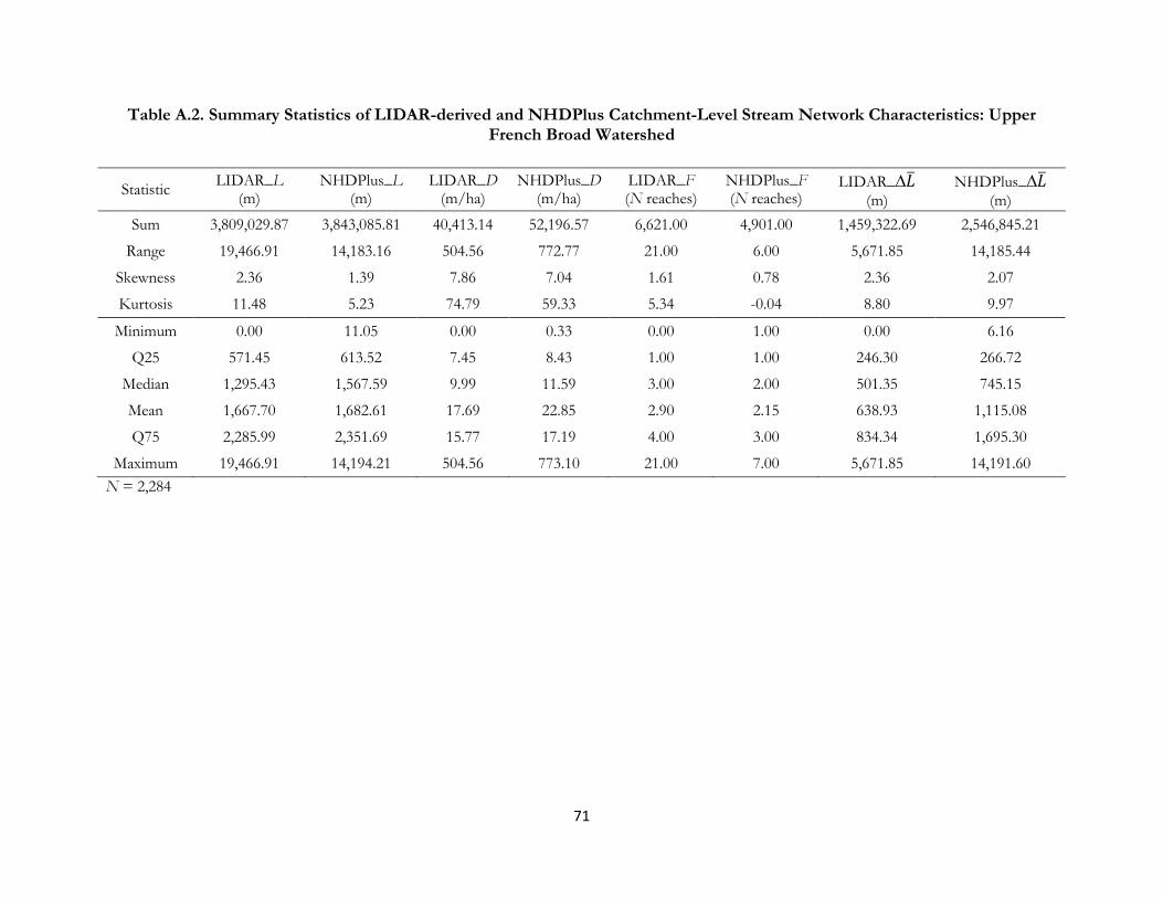
71

Table A.2. Summary Statistics of LIDAR-derived and NHDPlus Catchment-Level Stream Network Characteristics: Upper French Broad Watershed

Statistic LIDAR_L

(m) NHDPlus_L

(m) LIDAR_D

(m/ha) NHDPlus_D

(m/ha) LIDAR_F (N reaches)

NHDPlus_F (N reaches)

LIDAR_∆ (m)

NHDPlus_∆ (m)

Sum 3,809,029.87 3,843,085.81 40,413.14 52,196.57 6,621.00 4,901.00 1,459,322.69 2,546,845.21

Range 19,466.91 14,183.16 504.56 772.77 21.00 6.00 5,671.85 14,185.44

Skewness 2.36 1.39 7.86 7.04 1.61 0.78 2.36 2.07

Kurtosis 11.48 5.23 74.79 59.33 5.34 -0.04 8.80 9.97

Minimum 0.00 11.05 0.00 0.33 0.00 1.00 0.00 6.16

Q25 571.45 613.52 7.45 8.43 1.00 1.00 246.30 266.72

Median 1,295.43 1,567.59 9.99 11.59 3.00 2.00 501.35 745.15

Mean 1,667.70 1,682.61 17.69 22.85 2.90 2.15 638.93 1,115.08

Q75 2,285.99 2,351.69 15.77 17.19 4.00 3.00 834.34 1,695.30

Maximum 19,466.91 14,194.21 504.56 773.10 21.00 7.00 5,671.85 14,191.60

N = 2,284

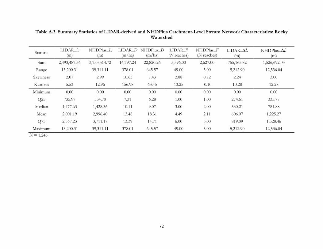
72

Table A.3. Summary Statistics of LIDAR-derived and NHDPlus Catchment-Level Stream Network Characteristics: Rocky Watershed

Statistic LIDAR_L

(m) NHDPlus_L

(m) LIDAR_D

(m/ha) NHDPlus_D



LIDAR_∆ (m)

NHDPlus_∆ (m)

Sum 2,493,487.36 3,733,514.72 16,797.24 22,820.26 5,596.00 2,627.00 755,165.82 1,526,692.03

Range 13,200.31 39,311.11 378.01 645.57 49.00 5.00 5,212.90 12,536.04

Skewness 2.07 2.99 10.65 7.43 2.88 0.72 2.24 3.00

Kurtosis 5.53 12.96 156.98 63.45 13.25 -0.10 10.28 12.28

Minimum 0.00 0.00 0.00 0.00 0.00 0.00 0.00 0.00

Q25 735.97 534.70 7.31 6.28 1.00 1.00 274.61 335.77

Median 1,477.63 1,428.36 10.11 9.07 3.00 2.00 530.21 781.88

Mean 2,001.19 2,996.40 13.48 18.31 4.49 2.11 606.07 1,225.27

Q75 2,567.23 3,711.17 13.39 14.71 6.00 3.00 819.09 1,528.46

Maximum 13,200.31 39,311.11 378.01 645.57 49.00 5.00 5,212.90 12,536.04

N = 1,246

73

Table A.4. Summary Statistics of LIDAR-derived and NHDPlus Catchment-Level Stream Network Characteristics: Pamlico Watershed

Statistic LIDAR_L

(m) NHDPlus_L

(m) LIDAR_D

(m/ha) NHDPlus_D



LIDAR_∆ (m)

NHDPlus_∆ (m)

Sum 2,620,117.11 1,463,159.42 17,118.75 25,010.56 2,917.00 3,256.00 652,648.48 848,124.59

Range 126,328.76 7,632.08 499.38 740.41 78.00 101.00 4,383.27 6,556.70

Skewness 11.10 1.32 7.31 5.93 7.91 10.13 1.62 2.00

Kurtosis 166.48 2.04 68.17 41.01 94.05 142.26 3.49 5.36

Minimum 0.00 9.55 0.00 0.08 0.00 1.00 0.00 2.68

Q25 224.63 463.36 4.23 6.34 1.00 1.00 144.18 188.33

Median 982.97 1,188.29 9.22 10.49 2.00 2.00 482.32 582.03

Q75 2,605.67 2,136.76 15.72 18.34 3.00 3.00 953.78 1,198.54

Mean 2,660.02 1,485.44 17.38 25.39 2.96 3.31 662.59 861.04

Maximum 126,328.76 7,641.63 499.38 740.49 78.00 102.00 4,383.27 6,559.38

N =985

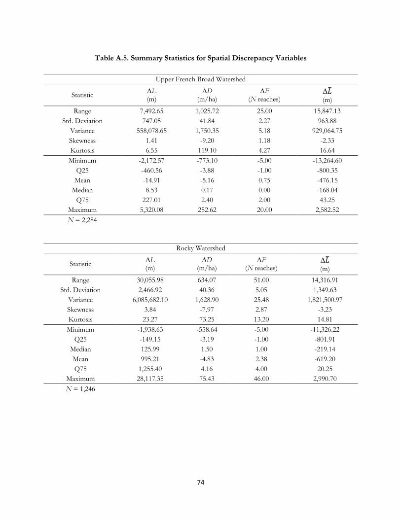
74

Table A.5. Summary Statistics for Spatial Discrepancy Variables

Upper French Broad Watershed

Statistic ∆L (m)

∆D (m/ha)

∆F (N reaches)

∆

(m)

Range 7,492.65 1,025.72 25.00 15,847.13

Std. Deviation 747.05 41.84 2.27 963.88

Variance 558,078.65 1,750.35 5.18 929,064.75

Skewness 1.41 -9.20 1.18 -2.33

Kurtosis 6.55 119.10 4.27 16.64

Minimum -2,172.57 -773.10 -5.00 -13,264.60

Q25 -460.56 -3.88 -1.00 -800.35

Mean -14.91 -5.16 0.75 -476.15

Median 8.53 0.17 0.00 -168.04

Q75 227.01 2.40 2.00 43.25

Maximum 5,320.08 252.62 20.00 2,582.52

N = 2,284

Rocky Watershed

Statistic ∆L (m)

∆D (m/ha)

∆F (N reaches)

∆

(m)

Range 30,055.98 634.07 51.00 14,316.91

Std. Deviation 2,466.92 40.36 5.05 1,349.63

Variance 6,085,682.10 1,628.90 25.48 1,821,500.97

Skewness 3.84 -7.97 2.87 -3.23

Kurtosis 23.27 73.25 13.20 14.81

Minimum -1,938.63 -558.64 -5.00 -11,326.22

Q25 -149.15 -3.19 -1.00 -801.91

Median 125.99 1.50 1.00 -219.14

Mean 995.21 -4.83 2.38 -619.20

Q75 1,255.40 4.16 4.00 20.25

Maximum 28,117.35 75.43 46.00 2,990.70

N = 1,246

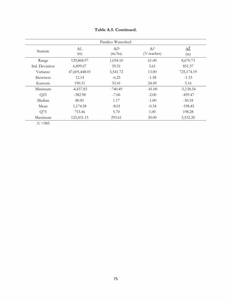
75

Table A.5. Continued.

Pamlico Watershed

Statistic ∆L (m)

∆D (m/ha)

∆F (N reaches)

∆

(m)

Range 129,868.97 1,034.10 61.00 8,670.73

Std. Deviation 6,899.67 59.51 3.61 851.57

Variance 47,605,448.01 3,541.72 13.00 725,174.19

Skewness 12.14 -6.25 -1.58 -1.33

Kurtosis 190.31 55.41 24.49 5.16

Minimum -4,437.83 -740.49 -41.00 -5,138.54

Q25 -382.98 -7.06 -2.00 -459.47

Median 80.81 1.17 -1.00 -30.18

Mean 1,174.58 -8.01 -0.34 -198.45

Q75 753.46 5.70 1.00 198.28

Maximum 125,431.15 293.61 20.00 3,532.20

N =985

76

Table A.6. Nonparametric Correlations of Landscape Characteristics and Catchment Areas

Landscape Variable

UFB

ROC

PAM


Catchment Area (ha)

Catchment Area (ha)

Catchment Area (ha)

Canopy .256** .038 .265** Rho

.000 .810 .000 Sig. (2-tailed)

Slope .377** .037 -.010

Rho

.000 .188 .757

Sig. (2-tailed)

Developed .058** .058** .058**

Rho

.005 .005 .005

Sig. (2-tailed)

Forest .203** .203** .203**

Rho

.000 .000 .000

Sig. (2-tailed)

Agriculture .007 .007 .007

Rho

.734 .734 .734

Sig. (2-tailed)

Water -.057** -.057** -.057**

Rho

.007 .007 .007

Sig. (2-tailed)

Aspect_N -.050* -.101** -.029

Rho

.017 .000 .369

Sig. (2-tailed)

Aspect_NE -.038 -.078** .179**

Rho

.067 .006 .000

Sig. (2-tailed)

Aspect_E .004 .099** .000

Rho

.853 .000 .989

Sig. (2-tailed)

Aspect_SE .046* .082** -.058

Rho

.029 .004 .070

Sig. (2-tailed)

Aspect_S -.068** -.129** -.061

Rho

.001 .000 .055

Sig. (2-tailed)

Aspect_SW .010 -.066* .143**

Rho

.636 .020 .000

Sig. (2-tailed)

Aspect_W .047* .033 -.093**

Rho

.023 .238 .003

Sig. (2-tailed)

Aspect_NW .011 .033 -.127**

Rho

.594 .243 .000

Sig. (2-tailed)

Note: Landscape metrics are defined in Section “”. Significant results are boldfaced. **Significant at 95

percent confidence. *Significant at 90 percent confidence.

77

Vita

Nicole Marie Samu received her B.A. in Psychology in 2005 from the University of Tennessee, Knoxville (UTK). She decided to pursue a career in geography shortly thereafter and earned her B.A. in Geography from UTK in 2008. Upon graduation, Nicole contracted with the Higher Education Research Experience (HERE) program at Oak Ridge National Laboratory (ORNL) and worked for the Geographic Information Science and Technology (GIST) Group; this opportunity allowed her to explore different research topics and to gain valuable professional experience. Nicole developed a strong interest for learning how GIS can be used to understand and address water resource issues and decided to pursue this interest for her graduate research at UTK. Upon graduation, Nicole hopes to continue gaining experience in geospatial data analysis and environmental research.

Spatial Discrepancies between NHDPlus and LIDAR-Derived Stream Networks

Documents

Transcript of Spatial Discrepancies between NHDPlus and LIDAR-Derived Stream Networks