Spatial Calibration and Temporal Validation of Flow for ... · PDF fileSPATIAL CALIBRATION AND...

SPATIAL CALIBRATION AND TEMPORAL VALIDATION OFFLOW FOR REGIONAL SCALE HYDROLOGIC MODELING1

C. Santhi, N. Kannan, J. G. Arnold, and M. Di Luzio2

ABSTRACT: Physically based regional scale hydrologic modeling is gaining importance for planning and man-agement of water resources. Calibration and validation of such regional scale model is necessary before applyingit for scenario assessment. However, in most regional scale hydrologic modeling, flow validation is performed atthe river basin outlet without accounting for spatial variations in hydrological parameters within the subunits.In this study, we calibrated the model to capture the spatial variations in runoff at subwatershed level to assurelocal water balance, and validated the streamflow at key gaging stations along the river to assure temporal vari-ability. Ohio and Arkansas-White-Red River Basins of the United States were modeled using Soil and WaterAssessment Tool (SWAT) for the period from 1961 to 1990. R2 values of average annual runoff at subwatershedswere 0.78 and 0.99 for the Ohio and Arkansas Basins. Observed and simulated annual and monthly streamflowfrom 1961 to 1990 is used for temporal validation at the gages. R2 values estimated were greater than 0.6. Insummary, spatially distributed calibration at subwatersheds and temporal validation at the stream gagesaccounted for the spatial and temporal hydrological patterns reasonably well in the two river basins. This studyhighlights the importance of spatially distributed calibration and validation in large river basins.

(KEY TERMS: spatially distributed calibration; validation; hydrologic modeling; regional scale; HUMUS; SWAT;CEAP.)

Santhi, C., N. Kannan, J.G. Arnold, and M. Di Luzio, 2008. Spatial Calibration and Temporal Validation of Flowfor Regional Scale Hydrologic Modeling. Journal of the American Water Resources Association (JAWRA) 44(4):829-846. DOI: 10.1111 ⁄ j.1752-1688.2008.00207.x

INTRODUCTION

There are serious concerns about managing thewater quantity and quality throughout the UnitedStates (U.S.) (USEPA, 1998). As water resourcesystems often cross local and state boundaries, theplanning and management processes often require a

basin-wide or regional perspective. Compared to thetraditional approach of looking at a specificwatershed, a regional planning approach can help todevelop a comprehensive vision for future growth,and develop plans to use and manage the waterresources efficiently. However, management and utili-zation of water resources in a region depends uponthe spatial and temporal distribution of rainfall,

1Paper No. J06179 of the Journal of the American Water Resources Association (JAWRA). Received December 16, 2006; accepted February20, 2008. ª 2008 American Water Resources Association. No claim to original U.S. government works. Discussions are open untilFebruary 1, 2009.

2Respectively (Santhi, Kannan, Di Luzio) (Associate Research Scientist, Assistant Research Scientist, Research Scientist), BlacklandResearch and Extension Center, Texas A&M University System, 720 East Blackland Road, Temple, Texas 76502; and Supervisory Agricul-tural Engineer and Research Leader, Grassland Soil and Water Research Laboratory, Agricultural Research Service-U.S. Department ofAgriculture, 808 East Blackland Road, Temple, Texas 76502 (E-Mail ⁄ Santhi: [email protected]).

JOURNAL OF THE AMERICAN WATER RESOURCES ASSOCIATION 829 JAWRA

JOURNAL OF THE AMERICAN WATER RESOURCES ASSOCIATION

Vol. 44, No. 4 AMERICAN WATER RESOURCES ASSOCIATION August 2008

runoff, ground-water storage, evapotranspiration (ET),soil types and crops grown. These factors vary frombasin to basin or region to region. Therefore, under-standing and capturing the spatial and temporal vari-ability of these factors on hydrological pattern both atsubwatershed and watershed levels is necessary.

Physically based regional scale hydrologic modeling(with geographic information system [GIS] capability)can simulate the spatial and temporal variability ofhydrological processes in different subunits of theregion. It can be used for investigating the impacts ofdifferent water quality management alternatives indifferent subunits and develop management plans.However, development of regional scale models is adifficult task, because of the spatial and temporalscales that must be considered and the large amountof information that must be integrated. The other dif-ficult task is the calibration of the model at regionalscale. Only limited attempts had been made todevelop, apply, and validate physically based hydro-logical models for regional scale studies.

Jha et al. (2006) have used physically based model,Soil and Water Assessment Tool (SWAT) in combina-tion with General Circulation Model for regional scaleclimate studies in the U.S. Hao et al. (2004) modeledthe Yellow River Basin in China and calibrated andvalidated the flow. In most regional or large-scalemodeling studies including the above, simulated flowis calibrated and validated against measured stream-flow at one or two gaging stations on the river mostlyat the watershed outlet. This is accomplished byadjusting the model inputs for the entire watershedto match the flows at the selected gages withoutadequate validation in various subunits or subwater-sheds of the region. One of the major limiting factorsfor this is the availability of observed flow data forcalibration and validation. However, it is importantto note that there are wide variations in runoff pro-duced in different subunits of the large river basindue to variations in rainfall, soils, land use and vege-tation and the associated hydrological processes. It isnecessary to capture the spatial and temporal vari-ability of hydrologic pattern across the region withadequate calibration of runoff in different subunits(Arnold et al., 2000) and also the temporal variationsof flow patterns. Runoff being an important compo-nent of the water balance, capturing the variation inrunoff will represent the hydrologic pattern in thewatershed. Qi and Grunwald (2005) have calibratedand validated the simulated flow against measuredstream flow in the Sandusky watershed at thewatershed outlet and four other subwatershed loca-tions using SWAT. Their approach captured the spa-tial and temporal variations in flow in the foursubwatersheds and the watershed. Their study wasconducted on a relatively small watershed (drainage

area 3,240 km2) and calibration and validation wasconducted for two years each.

The calibration and validation approach used inthis study is different from the above studies. Thespecific objectives of this study are to conduct:

(1) a spatially distributed calibration of long-termaverage annual runoff at subwatershed level ina regional scale river basin to capture the spa-tial variation in runoff in different parts of theriver basin, and

(2) a temporal validation of streamflow at key loca-tions (gage) along the river.

The spatial calibration helps in assuring localwater balance at subwatershed level. The temporalvalidation is performed to assure annual and sea-sonal variability. It is expected that the calibrationand validation approach used for large river basinsin this study would improve the reliability of hydro-logic model predictions in regional scale river basinsand also would improve our knowledge of localhydrological patterns nested within a large basin.This approach would also be useful for modelers,researchers and planners involved in regional scalestudies.

This study was conducted as part of an on-goingnational scale assessment study, Conservation EffectsAssessment Project (CEAP). CEAP follows theHUMUS ⁄ SWAT (Hydrologic Unit Modeling for theU.S.) watershed modeling framework (Srinivasanet al., 1998). Within the HUMUS framework eachwater resource region (major river basin) is treatedas a watershed and each U.S. Geological Survey(USGS) delineated eight-digit watershed as asub-watershed for use in SWAT modeling. TheHUMUS system is updated with recently availabledatabases and SWAT model for the CEAP—NationalAssessment (Santhi et al., 2005; Di Luzio et al.,2008). The main objective of the CEAP study is toquantify the environmental and economic benefitsobtained from the conservation practices and pro-grams implemented in the U.S. The benefits arereported at the eight-digit watershed and river basinscales. Therefore, the hydrologic model used for suchassessment is expected to simulate the flow and pol-lutant transfer reasonably well in all the eight-digitwatersheds and time series of streamflow at key loca-tions along the main river system. The regional scalecalibration and validation approach described in thisstudy is used for CEAP. This paper describes theregional scale hydrologic modeling and spatial andtemporal calibration and validation of flow in tworiver basins with different hydrologic conditions (ahigh flow and a low flow region based on annualaverage rainfall and runoff).

SANTHI, KANNAN, ARNOLD, AND DI LUZIO

JAWRA 830 JOURNAL OF THE AMERICAN WATER RESOURCES ASSOCIATION

METHODOLOGY

The CEAP ⁄ HUMUS system used in this study con-sists of a hydrologic ⁄ watershed scale model, SWAT(Arnold et al., 1998; Neitsch et al., 2002; http://www.brc.tamus.edu/swat) and revised databases forpreparing the model inputs (Santhi et al., 2005; DiLuzio et al., 2008). SWAT was selected because of itsability to simulate land management processes inlarge watersheds. SWAT has been widely used in theU.S. and other countries (Arnold et al., 1999; Borahand Bera, 2004; Gassman et al., 2007). Arnold et al.(1999) and Gassman et al. (2007) have reported previ-ous model validation studies of several locationsthroughout the U.S. Borah and Bera (2004) haveextensively reviewed various models and indicatedthat SWAT is a suitable model for long-term continu-ous simulations of large watersheds.

SWAT Model Description

SWAT is a physically based, semi-distributedmodel developed to simulate continuous-time land-scape processes and streamflow with a high level ofspatial detail by allowing the river ⁄ watershed to bedivided into a large number of subbasins or sub-watersheds. Each subbasin is further divided intoseveral unique land use and soil combinations calledHydrologic Response Units (HRUs) based on thresh-old percentages used to classify the land use and soil(Arnold et al., 1998; Neitsch et al., 2002) and they arehomogeneous. SWAT operates on a daily time stepand is designed to simulate water, sediment and agri-cultural chemical transport in a large ungaged basinand evaluate the effects of different management sce-narios on watershed hydrology and point and non-point source pollution. Key components of the modelinclude hydrology, weather, erosion, soil temperature,crop growth, nutrients, pesticides, and agriculturalmanagement. A complete description of all compo-nents can be found in Arnold et al. (1998) andNeitsch et al. (2002). A brief description on flow isprovided here.

Upland Processes ⁄ Hydrology. The local waterbalance in the Hydrologic Response Unit is providedby four storage volumes: Snow (stored volume untilit melts), soil profile (typically 0-2 m), shallow aqui-fer (typically 2-20 m), and deep aquifer (>20 m). Thesoil profile can be subdivided into multiple layers.Soil water processes include infiltration, runoff,evaporation, plant uptake, lateral flow, and percola-tion to lower layers. Percolation from the bottom ofthe soil profile recharges the shallow aquifer

(ground-water recharge). Surface runoff from dailyrainfall is estimated with a modification of U.S.Department of Agriculture-Soil Conservation Service(SCS) curve number method (USDA-SCS, 1972).Green & Ampt infiltration method is also availablewithin SWAT to simulate surface runoff and infiltra-tion. SWAT has options to estimate the potentialevapotranspiration (PET) by different methods suchas Modified Penman Montieth, Hargreaves, andPriestley-Taylor. The Hargreaves method is used inthis study (Hargreaves et al., 1985). Flow genera-tion, sediment yield and nonpoint source loadingsfrom each HRU in a subwatershed are summed andthe resulting flow and pollutant loads are routedthrough channels, reservoirs and ⁄ or ponds to thewatershed outlet.

Channel Processes. Channel processes simulatedwithin SWAT include flood routing, sediment routingand nutrient and pesticide routing. Ponds ⁄ Reservoirscomponents including water balance, routing, sedi-ment settling and simplified nutrient and pesticidetransformation are used in SWAT (Neitsch et al.,2002).

Study Area Description

Two river basins or water resources regions withdifferent climatic conditions, runoff, land use distri-bution, vegetation, soils, and topography have beenmodeled to capture the spatial and temporal varia-tions involved in the hydrologic processes and demon-strate the validity of the regional ⁄ basin scalemodeling effort. The two regions studied are as fol-lows: (1) The Ohio River Basin located in the easternU.S., and (2) The Arkansas-White-Red River Basinlocated in the south central U.S. (Figure 1). Thesetwo regions are also referred to as Region 05 andRegion 11 by the USGS at a 2-digit watershed scaleor hydrologic accounting unit.

Ohio River Basin. The Ohio River starts at theconfluence of the Allegheny and the Monongahela inPittsburgh, Pennsylvania, and ends in Cairo, Illinois,where it flows into the Mississippi River. It flowsthrough six states: Pennsylvania, West Virginia,Ohio, Illinois, Indiana and Kentucky (Figure 1).There are several dams across the Ohio River includ-ing many lock and dams built to facilitate navigation.The region is comprised of 120 USGS delineatedeight-digit watersheds. The Ohio River Basin receivesa high amount of rainfall. Agriculture is the predomi-nant land use in this region and about 21% of theland is used as cropland (Table 1). The predominantsoils in the region are gilpin, hazleto, zanesview,

SPATIAL CALIBRATION AND TEMPORAL VALIDATION OF FLOW FOR REGIONAL SCALE HYDROLOGIC MODELING


faywood, and bodine (USDA-NRCS, 1994). Thisregion has also witnessed increased populationgrowth, urbanization and industrial development.

Nonpoint source pollution from agricultural activitiesand urban runoff are major sources of pollution inthis river basin.

FIGURE 1. The Ohio and Arkansas-White-Red River Basins in the Conterminous United States With Flow Validation Gaging Stations.

TABLE 1. Watershed Characteristics of Ohio and Arkansas-White-Red River Basins.

River Basins ⁄ Regions Ohio River Basin (Region 05)Arkansas-White-Red River Basin

(Region 11)

Number of eight-digit watersheds 120 173Average annual rainfall at eight-digitwatersheds* (mm)

1,140 800

Estimated average annual PET and ETat eight-digit watersheds* (mm)

1,100 and 700 1,500 and 600

Estimated average annual runoff ateight-digit watersheds* (mm)

440 150

Predominant land uses (%) Forest (51%), Pasture ⁄ Hay (22%),Cropland (21%), Urban (3%) and others (3%)

Range (41%), Forest (22%), Pasture ⁄ Hay(19%), Cropland (14%) and others (4%)

*Average values of 30 years, approximated or rounded off.



Arkansas-White-Red River Basin. The drain-age area of this region includes (1) the ArkansasRiver, within and between the States of Colorado,Kansas, Oklahoma, and Arkansas; (2) the WhiteRiver, within and between the States of Missouri andArkansas; and (3) the Red River, within and betweenthe States of New Mexico, Texas, and Louisiana (Fig-ure 1). These major rivers flow generally from west toeast. The region is comprised of 173, eight-digitwatersheds. Although most of the regions are domi-nated by range and forest, about 14% of the land isused for growing crops (Table 1). Dominant soils inthe region are carnasa, stephen, berda, clarksv, duni-pha, enders, pullman, and manvel (USDA-NRCS,1994). The prevalent water quality problem in thisregion is from nonpoint source pollution. Sedimentand nutrients are the major causes of nonpointsource pollution, especially in the State of Oklahoma.Some of the largest poultry and swine operations inthe U.S. are located in this region. The impacts havebecome more prevalent in the streams, rivers, andlakes. Many of these lakes are the major drinkingwater source for large cities in this region.

Databases and Model Inputs

The HUMUS ⁄ SWAT system requires several datasuch as land use, soils, management practices,weather, point source data, and reservoirs. Consider-able effort has been made to process and update theHUMUS ⁄ SWAT databases for CEAP and prepareSWAT input files for the river basins (Santhi et al.,2005; Di Luzio et al., 2008). The various databasesused are described here.

Land Use. The 1992 USGS—National Land CoverDataset at 30 m resolution was used in this studyand it included land use classes such as cropland(row ⁄ small grains), urban, pasture, range, forest, wet-land, barren, and water. Land use-related informa-tion is input to the model at HRU level.

Soils. Each land use within a subbasin is associ-ated with soil data. Soil data required for SWAT wereprocessed from the State Soil Geographic (STATSGO)database (USDA-NRCS, 1994). Each STATSGO poly-gon contains multiple soil series and the aerial per-centage of each soil series. The soil series with thelargest area was extracted and the associated physi-cal properties of the soil series were used. Soil prop-erties used in modeling include texture, bulk density,saturated hydraulic conductivity, available waterholding capacity (AWC), total depth of soil, andorganic carbon. Soil information is input for eachHRU.

Management Data. Management operations,such as planting, harvesting, applications of fertili-zers, manure, and pesticides and irrigation water andtillage operations are used for various land uses inthe management files. A crop parameter databaseavailable within SWAT (Neitsch et al., 2002) is usedto characterize and simulate the crop growth definedin the management file. Management information isinput at HRU level.

Topography. Elevation information is used todelineate the watersheds into different subwater-sheds. Accumulated drainage area, overland fieldslope, overland field length, channel dimensions,channel slope, and channel length are derived foreach subwatershed using the 3-arc second digital ele-vation model (DEM) data (Srinivasan et al., 1998).Information extracted from DEM is used at subwater-shed and HRU levels.

Weather. Measured daily precipitation and maxi-mum and minimum temperature data from 1960 to2001 are used in this study. The precipitation andtemperature datasets are newly created (Di Luzioet al., 2008) from a combination of point measure-ments of daily precipitation and temperature (maxi-mum and minimum) (Eischeid et al., 2000) andPRISM (Parameter-elevation Regressions on Indepen-dent Slopes Model) (Daly et al., 2002). The point mea-surements compose serially complete (withoutmissing values) dataset processed from the stationrecords of the National Climatic Data Center. PRISMis an analytical model that uses point data and a dig-ital elevation model to generate gridded estimates ofmonthly climatic parameters and distributed at4 km2. Di Luzio et al. (2008) have developed a novelapproach to combine the point measurements and themonthly PRSIM grids to develop the distribution ofthe daily records with orographic adjustments overeach of the USGS eight-digit watersheds. Other datasuch as solar radiation, wind speed and relativehumidity are simulated using the monthly weathergenerator parameters from weather stations (Nicks,1974; Sharpley and Williams, 1990) available withinSWAT database for these regions. Weather data areinput for each subwatershed.

Point Source Data. Effluents discharged fromthe municipal treatment plants are major pointsources of pollution. The USGS has developed a pointsource database for use in the SPARROW (SPAtiallyReferenced Regressions On Watershed attributes)model simulations (Smith et al., 1997) and it is usedin this study. Point source data used include effluentdischarge ⁄ flow and sediment and nutrient loadings.Point source data are input at subwatershed level.



The point source data was updated for 2000 popula-tion.

Reservoirs. Basic reservoir data such as storagecapacity and surface area were obtained from thedams database (U.S. Army Corps of Engineers, 1982;Hitt, 1985). Because of the lack of adequate reservoirrelease data and complexity involved in simulatingeach reservoir operation in large-scale modelingeffort, a simple reservoir simulation approach avail-able within the SWAT model is used with a monthlytarget release-storage approach based on the storagecapacity and flood and nonflood seasons (Neitschet al., 2002). Reservoir related data are input at thesubwatershed level.

Calibration and Validation Approach Used forRegional Scale Hydrologic Modeling

For this regional scale modeling, a calibration pro-cedure involving (1) calibration of spatial variationsin runoff at subwatershed level, and (2) temporal val-idation of streamflow at multiple gaging stationsalong the major river, was used. The model was runusing weather data from 1960 through 1990 for thetwo river basins studied. Data from 1960 is used forthe model to assume realistic initial conditions and itwas not included in the calibration. Data from 1961-1990 is used for calibration. Subwatersheds andeight-digit watersheds are used interchangeably inthis paper.

Spatially Distributed Calibration. In general,spatial calibration refers to the calibration of awatershed model with known ‘‘spatially distributed’’input and output information. SWAT is a physicallybased, semi-distributed watershed model and thewatershed is disaggregated in geographical spaceand their processes in time. Thus, analysis can bedescribed in a spatial and temporal context. Sub-watershed is considered as the ‘‘spatial unit of vari-ation’’ for this regional scale calibration studybecause this is a relatively large area study to meetthe needs of the CEAP national assessment. From awatershed modeling perspective, SWAT is capable ofsimulating a high level of spatial detail by allowinga watershed to be divided into multiple subwater-sheds. Heterogeneity in inputs within a subwater-shed is captured by dividing the subwatershed intoseveral HRUs, which are unique land use soil com-binations. More land use and soil combinations(more HRUs for increased spatial detail) within asubwatershed can be obtained by using the lowestthreshold level for selecting land use and soilcombinations.

Observed data used for spatially distributed cali-bration: Gebert et al. (1987) has prepared the averageannual runoff contour map for the conterminousUnited States using measured streamflow data from5,951 USGS gaging stations for the period 1951-1980and the stream flows at these gauging stations wereconsidered to be natural (i.e., unaffected by upstreamreservoirs or diversions) and representative of localconditions. For this study, the contours of averageannual runoff produced by Gebert et al. (1987) wereinterpolated to produce a smooth grid using GISinterpolation technique called inverse distanceweighting and the average annual runoff for eight-digit watersheds were estimated. Although the runoffestimated is long-term annual average, it was stillused for calibration to capture the spatial variationsin runoff at subwatershed level because of a large(regional) study area, adequacy of the project needs,and limitation in availability of time series observeddata. The average annual runoff is a good indicatorof annual water balance in a subwatershed orwatershed although it may not readily convey thetemporal variation effects and seasonality effects.Several studies have used the average runoff con-tours for regional scale studies and showed the spa-tial variation in runoff across the region (Wolock andMc Cabe, 1999). Hence, it is important to capture thespatial variation in runoff during calibration.

Calibration Parameters: The model is calibrated tocapture the spatial variation in long-term averageannual observed runoff by adjusting several modelinput parameters (Table 2), keeping them withinrealistic uncertainty ranges. Calibration is performedfor each subwatershed (eight-digit) by adjusting themodel parameters that capture the spatial and tem-poral variations in model inputs such as soils, landuse, topography, and weather and interactions amongthem influencing various hydrologic processes, suchas runoff, ET, and ground-water flow. The inputparameters used for calibration (Table 2) include

(1) HARG_PETCO is a coefficient used to adjustpotential evapotranspiration (PET) estimated byHargreaves method (Hargreaves and Samani,1985; Hargreaves and Allen, 2003) and calibratethe runoff in each subwatershed. In Hargreavesmethod, PET is related to temperature and ter-restrial radiation. This coefficient is related toradiation and can be varied to match the PETin different parts of the region depending on theweather conditions (Hargreaves and Allen,2003).

(2) Soil water depletion coefficient (CN_COEF) is acoefficient used in the curve number method toadjust the antecedent moisture conditions onsurface runoff. This parameter is related to



PET, precipitation and runoff in the curve num-ber method.

(3) Curve number (CN) is used to adjust surfacerunoff and relates to soil and land use andhydrologic condition at HRU level.

(4) Ground-water re-evaporation coefficient (GWR-EVAP) controls the upward movement of waterfrom shallow aquifer to root zone, due to waterdeficiencies, in proportion to PET. This para-meter can be varied depending on the landuse ⁄ crop. The revap process is significantin areas where deep rooted plants are growingand affects the groundwater and the waterbalance.

(5) GWQMN-minimum threshold depth of water inthe shallow aquifer to be maintained forground-water flow to occur to the main channel.

(6) Soil AWC, which varies by soil at HRU level.(7) Soil evaporation compensation factor (ESCO),

which controls the depth distribution of waterin soil layers to meet soil evaporative demand.This parameter varies by soil at HRU level.

(8) Plant evaporation compensation factor (EPCO),that allows water from lower soil layers to meet

the potential water uptake in upper soil layersand varies by soil at HRU level.

The input parameters were adjusted within litera-ture reported ranges (Santhi et al., 2001; Neitschet al., 2002). Additional details of these parameterscan be found in Neitsch et al. (2002). Effects of theseinput parameters on different components of runoffare shown in Table 2. It should be noted that anadjustment in runoff (due to changes in modelparameters) results in changes in surface runoffand ⁄ or groundwater. Similarly, changes in surfacerunoff and groundwater result in changes in runoff.

The calibration process for each eight-digitwatershed is carried out in three steps viz. (1) cali-bration of runoff (by adjusting HARG_PETCO), (2)surface runoff (by adjusting soil water depletion-coef-ficient and curve number), and (3) ground-water (allthe other parameters mentioned in Table 2). An auto-mated procedure is developed for conducting the spa-tially distributed calibration process at eight-digitwatersheds in the river basin (Kannan et al., 2008).Simulated runoff in each eight-digit watershed wascalibrated by adjusting the model input parameters

TABLE 2. Input Parameters Used in the Calibration Procedure, Their Range and Their Effects on Different Components of Runoff.

Parameter DescriptionSpatial Level of

Parameterization

Changes Range Used

SurfaceRunoff

GroundWater

WaterYield Min Max

HARG_PETCO Coefficient used to adjust potentialevapotranspiration estimated byHargreaves method and runoff

Subwatershed(HRU)

X X X 0.0019 0.0027

Soil WaterDepletionCoefficient(CN_COEF)

Coefficient used in the new curvenumber method (Neitsch et al., 2002;Kannan et al., 2008) and isused to adjust surface runoff andgroundwater in accordance with soilwater depletion.

Subwatershed(each soil in HRU)

X X X 0.5 1.50

CN Curve number—adjust surface runoff HRU (for eachlanduse and soil)

X X )5 +5

GWQMN Minimum threshold depth of waterrequired in shallow aquifer forground-water flow to occur

Subwatershed X X )3 +3

GWREVAP Groundwater re-evaporation coefficientthat controls the upward movementof water from shallow aquifer to rootzone in proportion to evaporativedemand

Subwatershed X X 0.02 0.20

AWC Soil available water holding capacity HRU X X )0.04 +0.04ESCO Soil evaporation compensation factor,

that is used to modify the depthdistribution of waterin soil layers to meet the soil evaporativedemand)

HRU X X 0.50 0.99

EPCO Plant evaporation compensation factor,that allows water from lower soil layersto meet the potential water uptakein upper soil layers

HRU X X 0.01 0.99



until average annual observed runoff and simulatedrunoff were within 20%. In this study, the simulatedrunoff (same as water yield) is defined as the sum ofsurface runoff, lateral flow from the soil profile andground-water flow from the shallow aquifer simulatedby the model. It is expected that this spatial calibra-tion procedure (with minimal or no additional calibra-tion) can provide good results in predictions ofannual and monthly flows.

Temporal Validation of Flow at MultipleGages Along the Main River. The temporal vali-dation approach is useful in evaluating the modelperformance during high and low flow years, annual,seasonal, and monthly variations and in understand-ing the long-term temporal variations in hydrologicprocesses. Such a long-term study is necessary forplanning and implementing conservation measuresand programs and evaluating their performance. Itshould be noted that minimal attempt was made toadjust the model parameters or do additional calibra-tion during temporal flow validation.

Observed data used for temporal validation:Annual and monthly streamflow data from USGSgaging stations at key locations along the main riverrepresenting different drainage area were selectedand used to validate the simulated flow to assureproper annual and seasonal variability (Figure 1 andTable 3).

Statistical measures used for model evaluation:Several statistical measures including mean, stan-dard deviation, coefficient of determination (R2) andNash-Suttcliffe efficiency (NSE) (Nash and Suttcliffe,1970) were used to evaluate the annual and monthlysimulated flows against the measured flows at thegages. If the R2 and NSE values are less than or veryclose to 0.0, the model prediction is considered ‘‘unac-ceptable or poor.’’ If the values are 1.0, then themodel prediction is considered ‘‘perfect.’’ A valuegreater than 0.6 for R2 and a value greater than 0.5for NSE, were considered acceptable (Santhi et al.,2001; Moriasi et al., 2007).

RESULTS AND DISCUSSION

Calibration of Spatial Variation in Runoff

Precipitation, simulated ET, simulated runoff, andobserved runoff for the Ohio and Arkansas regionsshow the variations in hydrological patterns acrosseight-digit watersheds (Figures 2 and 3). It was notedthat the observed runoff estimated at eight-digitwatersheds varied widely ranging from <200 mm

through 750 mm in the Ohio River Basin and it var-ied from <50 mm through 530 mm in the ArkansasRiver Basin. Hence, it is important to account for thisspatial variation in runoff across the subwatershedsas opposed to traditionally calibrating the modelinputs over the entire basin to match the flow at onestream gage at the watershed outlet. In order to illus-trate how some of the model input parameters spa-tially affect the simulated outputs (either runoff orsurface runoff or ground water), three such modelinput parameters are discussed here. Depending onthe type of land use, crops grown, soil types, precipi-tation, and evaporation in each subwatershed, effectsof these parameters on simulated hydrology (runoff,surface runoff, and ground water and ET) variedacross subwatersheds.

1. HARG_PETCO, is used to calibrate the runoff byadjusting the PET within each subwatershed.PET is related to maximum and minimum

TABLE 3. Summary of Validation Results for GagingStations in the Ohio and Arkansas-White-Red River Basins.

Region

Name Ohio Ark-White-Red

Region Region 05 Region 11

Gagedetails

River Ohio RedLocation Louisville, KY Index, ARStation ID 03294500 07337000Drain Area (km2) 236,130 124,398

Annual Mean (O) mm 451 87Mean (S) mm 433 75StdDev (O) mm 100 45StdDev (S) mm 82 42R2 0.94 0.86NSE 0.86 0.79

Monthly Mean (O) mm 38 7Mean (S) mm 36 6StdDev (O) mm 28 8StdDev (S) mm 20 7R2 0.83 0.66NSE 0.72 0.64

Gagedetails

River Ohio ArkansasLocation Metropolis, IL Arkansas City, KSStation ID 03611500 07146500Drain Area (km2) 525,770 113,217

Annual Mean (O) mm 491 14Mean (S) mm 467 10StdDev (O) mm 122 6StdDev (S) mm 100 7R2 0.95 0.71NSE 0.89 0.13

Monthly Mean (O) mm 41 1.3Mean (S) mm 39 1.0StdDev (O) mm 28 1.4StdDev (S) mm 22 2.0R2 0.83 0.64NSE 0.81 0.23

Notes: O, observed; S, simulated; StdDev, standard deviation.



temperature and radiation, which can vary spa-tially. Figure 4 shows the effects of HAR-GO_PETCO on simulated long-term annualaverage runoff in various subwatersheds (eight-digit) that were calibrated in the Ohio RiverBasin. Not all eight-digit watersheds requiredcalibration. Runoff increased in most of the sub-watersheds during calibration by reducing

HARG_PETCO to reduce PET. The magnitude ofincrease in runoff varied across subwatersheds(shown by bars in top, that is, difference in run-off before and after adjustment of HARG_PET-CO). Hargreaves method accounts for variationsin minimum and maximum temperature, andvariations in crops are accounted simultaneouslywhile estimating the actual ET.

FIGURE 2. Precipitation, Simulated ET, Simulated Runoff, and Observed Runoff for the Eight-Digit Watersheds in the Ohio River Basin.

FIGURE 3. Precipitation, Simulated ET, Simulated Runoff and ObservedRunoff for the Eight-Digit Watersheds in the Arkansas-White-Red River Basin.



FIGURE 4. Effect of HARG_PETCO on Spatial Variation in Simulated Runoffin the Eight-Digit Watersheds That Were Calibrated in the Ohio River Basin.

FIGURE 5. Effect of Soil Water Depletion Coefficient on Spatial Variation in Simulated Runoff and SurfaceRunoff in the Eight-Digit Watersheds That Were Calibrated in the Ohio River Basin (note: upward bars—decrease

and downward bars—increase in runoff and surface runoff after soil water depletion coefficient adjustment).



2. Soil water depletion coefficient (CN_COEF) isused for calibrating surface runoff in SWAT(Nietsch et al., 2002; Kannan et al., 2007b).Wang et al. (2006) indicated that surface runoffis sensitive to the soil water depletion coeffi-cient. It can be used to calibrate surface runoffand ground water proportions. The model over-estimated and underestimated surface runoff incertain eight-digit watersheds. Figures 5a and5b show the effects of the soil water depletioncoefficient on simulated runoff and surfacerunoff in various subwatersheds in the OhioRiver Basin. Magnitudes of the increase ordecrease in runoff and surface runoff variedacross subwatersheds (shown by upward anddownward bars) with changes in soil waterdepletion coefficient. It could be noticed thatchanges made in surface runoff and runoffshowed the trend to match the observed ortargeted runoff.

3. The spatial effects of ground-water re-evaporationcoefficient (GWREVAP) on long-term average

annual runoff and groundwater are shown in Fig-ures 6a and 6b. It could be noticed that thechanges observed in runoff were due to changes inground water in response to the GWREVAP coeffi-cient. The changes were up to 15 mm.

The other model input parameters were adjustedin the similar manner for runoff calibration in eacheight-digit watershed.

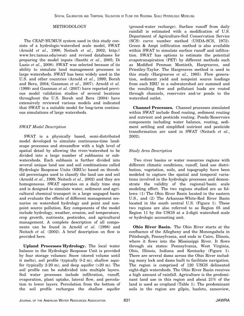
The average annual simulated runoff and averageannual observed runoff of the eight-digit watershedsin the Ohio region and Arkansas region are shown inFigures 7 and 8, respectively. In the Ohio region, theobserved runoff increased from northwest to thesoutheast similar to precipitation pattern (Figure 7).The simulated runoff showed similar pattern bycapturing the spatial variations in runoff across theregion (Figure 7). The regression relationshipbetween observed and simulated runoff at eight-digitwatersheds indicate that the model prediction is sat-isfactory (Figure 9a). Out of 120 hydrologic unit codes(HUCs) in the basin, the simulated runoff in 106

FIGURE 6. Effect of Ground-Water Revap Coefficient on Spatial Variation in Simulated Runoffand Ground Water in the Eight-Digit Watersheds That Were Calibrated in the Ohio River Basin.



HUCs were within 20% of the observed runoff. Therewere underpredictions of runoff in a few HUCs wherethe runoff was high in the range of 600-700 mm (Fig-ure 7). Further investigation showed that the modelunderpredicted the base flow portion in those HUCsthat were not matching the calibration criteria.Snowfalls and snowmelting are a common phenom-ena in the Ohio region and the model had difficultiesdealing with it.

FIGURE 7. Observed and Simulated Average AnnualRunoff for Eight-Digit Watersheds in the Ohio River Basin.

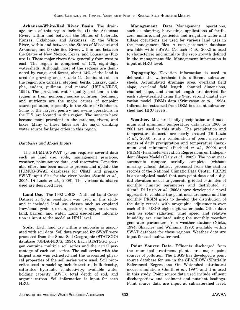
FIGURE 8. Observed and Simulated AverageAnnual Runoff for Eight-Digit Watershedsin the Arkansas-White-Red River Basin.



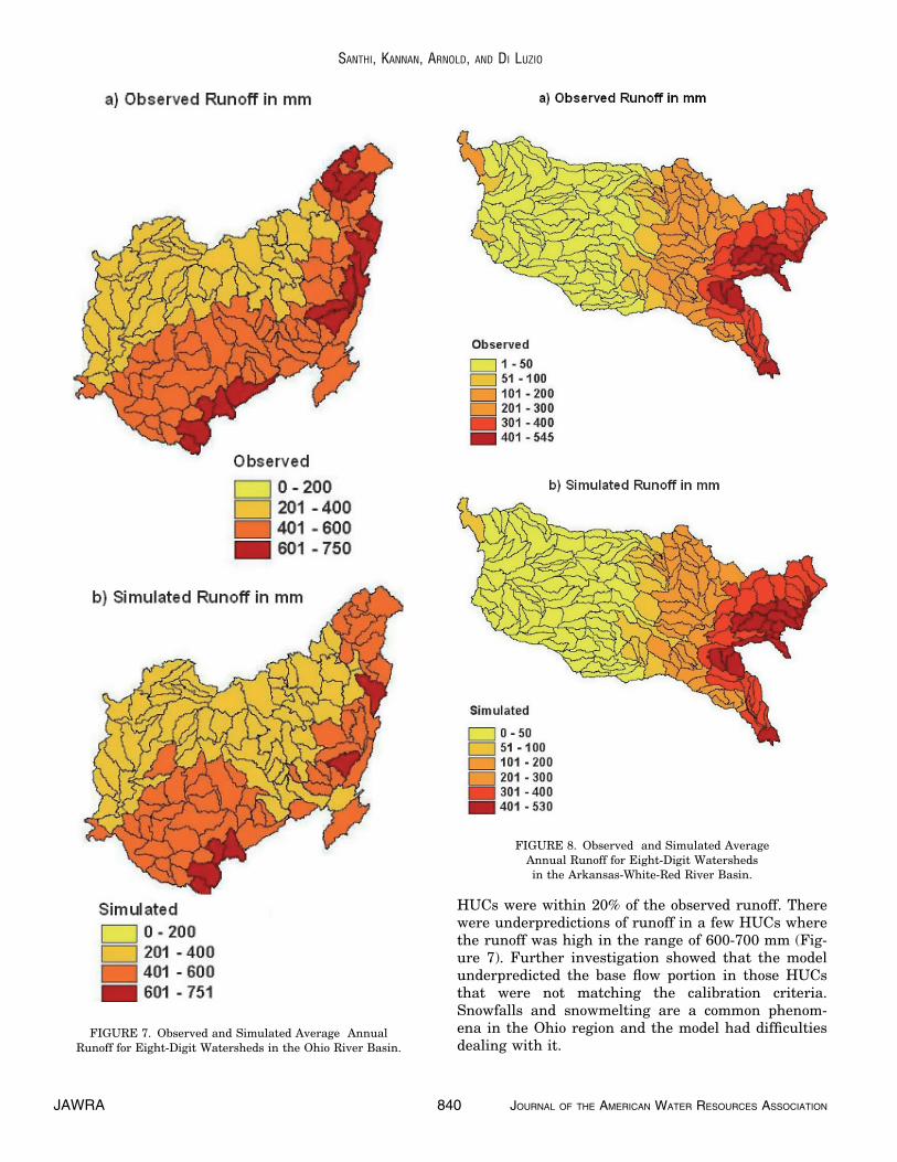
In the Arkansas-White-Red River region, the aver-age annual observed runoff varied widely from<50 mm in the western side through more than500 mm in the eastern side. Simulated runoffmatched this spatial variation pattern very well (Fig-ure 8). Observed and simulated runoff patterns are inconcurrence with the precipitation patterns of thisregion (Figure 3). The regression coefficient of 0.99(Figure 9b) revealed that the observed and simulatedrunoff matched very well at eight-digit watersheds inthis region. The simulated runoff was within 20% ofthe observed runoff in 128 HUCs out of 173 HUCs inthis region. As runoff is relatively low in majority ofthe HUCs in this region (Figure 8), considering theabsolute difference in runoff would be a better indica-tion than percentage difference. The simulated runoffwas within 25 mm in 159 HUCs and within of 50 mm

in 171 HUCs, when compared to the observed runoff(Figure 8).

Results of the two study regions indicate that theSWAT model is able to capture the spatial variationsin runoff and simulate the local water balances ade-quately.

Temporal Validation of Streamflow at MultipleGaging Locations in the Main River

Without further calibration, regression of observedand simulated annual and monthly streamflow wasperformed to validate the model.

Ohio River Basin: The observed and simulatedannual and monthly streamflows on the Ohio Riverat Louisville, Kentucky (USGS Station 03294500) andMetropolis, IL (USGS Station 03294500) matchedwell (Figure 10 and 11). Means of the observed andsimulated annual and monthly flows were within adifference of 10% at Louisville, Kentucky (Table 3).Further agreement between annual and monthly sim-ulated and observed flows at Louisville are shown bythe coefficient of determination >0.6 and NSE >0.5(Table 3). Good agreement between annual andmonthly observed, and simulated flows at Metropolis,Illinois, is indicated by the time series plots and sta-tistics (Figure 11 and Table 3). However, there is ageneral tendency for the model to underpredict thepeak flows during spring months and sometimesoverpredict the base flow during fall months. Thismay be due to either limitations in snowmelt simula-tion or simulation of the reservoir operations.

The Arkansas-White-Red River Basin: This is rela-tively a low flow region. The observed and simulatedannual and monthly streamflows along the ArkansasRiver at Arkansas City, Kansas (USGS Station07146500) matched moderately well except for over-prediction of peak flows (Figure 12) in a few yearsincluding 1973. As NSE is sensitive to outliers, theNSE computed was low because of the overestimationof peak flows. Further investigations revealed thatthere were major rainfall events during the monthsof March and October in 1973 and the model overpre-dicted the runoff events. Similarly, there was a con-sistent underprediction of the peaks duringMay ⁄ June in most of the years. The model was notable to simulate the sudden changes in flow varia-tions as seen in the observed flow. Hence, the simu-lated annual average flows were lower.

It could be observed from Figure 13a and statis-tics shown in Table 3 that the observed and simu-lated annual flows compared fairly well at Index onthe Red River, Arkansas (USGS Station 07337000).Simulated monthly flows were closer to the observedflows at this location (Figure 13b and Table 3).

FIGURE 9. Regression Relationship Between Average AnnualObserved and Simulated Runoff at Eight-Digit Watersheds

in the Ohio and Arkansas-White-Red River Basins.



Overall, the model preserved the peaks and reces-sions. In this region also, there is a general ten-dency for the model to underpredict peaks duringspring months.

It should be noticed that the mean annual flowvaried widely between the two regions (Figures 10-13).The mean annual streamflow at the gages analyzedin the Ohio River Basin were approximately 450 mmand while it varied from 15 to 90 mm in the Arkan-sas-White-Red River Region. Mean annual andmonthly flows at the two gaging stations in the OhioRiver Basin were in the similar ranges. However, inthe case of Arkansas-White-Red River Basin, therewere variations in mean annual flow between thegages at Arkansas City on the Arkansas River and atIndex on the Red river. The time series annual andmonthly flow results at the gages in both the regionsappeared to be reasonable given that no additionalcalibration was performed after the spatial runoffcalibration at eight-digit watersheds. Overall, themodel is able to capture the annual and monthly flowpatterns.

Results of runoff calibration at eight-digit water-sheds and streamflows at gaging stations indicatethat the hydrological variations at spatial and tempo-

ral scales are simulated reasonably well. This studyhas shown the importance of a spatial calibrationalong with temporal validation, especially when thereis a wide variation in runoff across the basin.Watershed characteristics within and between sub-watersheds differ in terms of precipitation, otherweather parameters, land use and land cover, topog-raphy, soils, and crops grown. These watershed char-acteristics generate variable hydrologic patternsacross the river basin. The calibration and validationapproach needs to capture the variations in flow pat-terns at subwatershed and watershed level for reli-able simulations of water flow. Reasonable accuracyin flow simulation is necessary for simulating thetransport of pollutants. Once the flow is estimatedreasonably well, the model can be calibrated and vali-dated for sediment and nutrients and can be used forseveral applications, including (1) identification ofsubwatersheds that have critical sediment ⁄ erosionproblems and, (2) identification of subwatersheds orwatershed region that contribute excessive nitrogenand phosphorus loadings to the river system, and (3)estimation of benefits of conservation practices onwater quality in terms of percentage reductions insediment, nutrients, and pesticide loadings. The

FIGURE 10. Annual and Monthly Observed and Simulated Flows at Louisville, Kentucky, on the Ohio River.



model can be also used to predict concentrations ofnitrogen and phosphorus in the river systems to meetwater quality standards for humans and eco-systemsand identify the sources of excessive nutrient contri-butions.

SUMMARY AND CONCLUSIONS

Physically based regional scale hydrologic model-ing is useful in investigating the effects of differentmanagement scenarios on water quality and quan-tity. Calibration and validation of the model for thestudy region are necessary to capture the variablehydrological patterns in subwatersheds and water-shed. This is especially important in large riverbasins with wide spatial and temporal variations inflow patterns. In addition, availability of limitedobserved data for model validation makes the regio-nal scale study challenging. In this study, regionalscale hydrologic modeling is described for two riverbasins, and a flow calibration ⁄ validation procedureinvolving calibration of spatial variation of annualaverage runoff at subwatershed level (to assure local

water balance), and validation of the time series offlow at key locations along the main river (to assuretemporal variability) is carried out using the SWAT.The regional scale modeling procedure is demon-strated with results from two river basins, the Ohioand Arkansas-White-Red River basins that are indifferent hydrologic conditions. The long-term aver-age annual runoff estimated from the USGS data forthe eight-digit watersheds were used for conductingthe spatially distributed calibration. R2 values ofaverage annual runoff at subwatersheds were 0.78and 0.99 for the Ohio and Arkansas Basins. Theannual and monthly streamflow data from the USGSgages from 1961-1990 were used for temporal flowvalidation. R2 values of the annual and monthlyflows for the multiple gaging stations studied at Ohioand Arkansas were >0.6. It is expected that the cali-bration and validation approach similar to this studywould improve the reliability of hydrologic modelpredictions at regional scale river basins. Because ofthe large-scale nature of the study and limitation inavailability of time series of observed data, averageannual runoff was used for spatial calibration. Theaverage annual runoff value is a good indicator ofwater balance in a subwatershed and this approachseemed to provide realistic prediction of the annual

FIGURE 11. Annual and Monthly Observed and Simulated Flows at Metropolis, Illinois, on the Ohio River.



FIGURE 12. Annual and Monthly Observed and Simulated Flows on theRed River at Index, Arkansas, in the Arkansas-White-Red River Basin.

FIGURE 13. Annual and Monthly Observed and Simulated Flows on the ArkansasRiver at Arkansas City, Kansas, in the Arkansas-White-Red River Basin.



and monthly flow pattern at multiple locations alongthe main river.

Major conclusions from this study include

(1) Compared to the traditional approach of cali-brating and validating at the watershed outlet,it is expected that the spatial calibration andvalidation approach would improve the reliabil-ity of hydrologic model predictions by capturingthe variations in flow patterns at subwatershedand watershed levels for large ⁄ regional scaleriver basins.

(2) When tested in two river basins, the spatial cal-ibration process seems to be helpful in capturingthe flow variations from low flow through highflow regimes. Reasonably accurate prediction offlow is a pre-requisite for reliable predictions ofsediment and nutrient yields.

(3) The application of spatial calibration and tempo-ral validation approach to large-scale studiescan be demonstrated with CEAP and ⁄ or otheragricultural management and water qualityprojects.

(4) Current regional scale modeling framework canbe used for potential applications such as toassess the effects of land use changes on waterquality and quantity, and assess the effects ofclimate changes on water budget at regionalscale. The modeling framework can also be usedby planners and managers to address severalpolicy-related questions on water supply andwater quality management issues.

ACKNOWLEDGMENTS

The USDA-NRCS Resource Inventory Assessment Division pro-vided funding for this work as part of the Conservation EffectsAssessment Project (CEAP). Thanks to the editor and the anony-mous reviewers for their constructive comments. The AgriculturalPolicy ⁄ Environmental extender (APEX) modeling team’s contri-bution is acknowledged.

LITERATURE CITED

Arnold, J.G., R.S. Muttiah, R. Srinivasan, and P.M. Allen, 2000.Regional Estimation of Baseflow and Groundwater Recharge inthe Upper Mississippi River Basin. Journal of Hydrology227:21-40.

Arnold, J.G., R. Srinivasan, R.S. Muttiah, and P.M. Allen, 1999.Continental Scale Simulation of the Hydrologic Balance. Jour-nal of the American Water Resources Association 35(5):1037-1051.

Arnold, J.G., R. Srinivasan, R.S. Muttiah, and J.R. Williams, 1998.Large Area Hydrologic Modeling and Assessment Part I: ModelDevelopment. Journal of the American Water Resources Associ-ation 34(1):73-89.

Borah, D.K. and M. Bera, 2004. Watershed Scale Hydrologic andNonpoint Source Pollution Models: Review of Applications.Transactions of the American Society of Agricultural Engineers47(3):789-803.

Daly, C., W.P. Gibson, G.H. Taylor, G.L. Johnson, and P. Pasteris,2002. A Knowledge Based Approach to the Statistical Mappingof Climate. Climate Research 22:99-113.

Di Luzio, M., G.L. Johnson, C. Daly, J. Eischeid, and J.G. Arnold,2008. Constructing Retrospective Gridded Daily Precipitationand Temperature Datasets for the Conterminous United States.Journal of Applied Meteorology and Climatology 47:475-497.

Eischeid, J.K., P.A. Pasteris, H.F. Diaz, M.S. Plantico, and N.J.Lott, 2000. Creating a Serially Complete, National Daily TimeSeries of Temperature and Precipitation for the Western UnitedStates. Journal of Applied Meteorology 39:1580-1591.

Gassman, P.W., M.R. Reyes, C.H. Green, and J.G. Arnold, 2007.The Soil and Water Assessment Tool: Historical Development,Applications and Future Research Directions. Transactions ofthe American Society of Agricultural and Biological Engineers50(4):1211-1250.

Gebert, W.A., D.J. Graczyk, and W.R. Krug, 1987. Average AnnualRunoff in the United States, 1951-1980. Hydrologic Investiga-tions Atlas, HA-70, U.S. Geological Survey, Reston, Virginia.

Hao, F.H., X.S. Zhang, and Z.F. Yang, 2004. A Distributed Non-point Source Pollution Model: Calibration and Validation in theYellow River Basin. Journal of Environmental Sciences16(4):646-650.

Hargreaves, G.L. and R.G. Allen, 2003. History and Evaluation ofHargreaves Evapotranspiration Equation. Journal of Irrigationand Drainage Engineering 129(1):53-63.

Hargreaves, G.L., G.H. Hargreaves, and J.P. Riley, 1985. Agricul-tural Benefits for Senegal River Basin. Journal of Irrigation andDrainage Engineering 111(2):113-124.

Hargreaves, G.H. and Z.A. Samani, 1985. Reference Crop Evapo-transpiration From Temperature. Applied Engineering in Agri-culture 1:96-99.

Hitt, K.J., 1985. Surface Water and Related Land Resources Devel-opment in the United States and Puerto Rico: U.S. GeologicalSurvey Special Map, Scale 1:3,168,000.

Jha, M., J.G. Arnold, P.W. Gassman, F. Giorgi, and R. Gu, 2006.Climate Change Sensitivity Assessment on Upper MississippiRiver Basin Streamflows Using SWAT. Journal of the AmericanWater Resources Association 42(4):997-1015.

Kannan, N., C. Santhi, and J.G. Arnold, 2008. Development of anAutomated Procedure for estimation of the spatial variation ofrunoff in large river basins. Journal of Hydrology (In reviewafter revision).

Kannan, N., C. Santhi, J.R. Williams, and J.G. Arnold, 2007.Development of a Continuous Soil Moisture Accounting Proce-dure for Curve Number Methodology and its Behaviour WithDifferent Evapotranspiration Methods. Hydrological Processes,doi: 10.1002 ⁄ hyp 6811.

Moriasi, D.N., J.G. Arnold, M.W. Van Liew, R.L. Bingner, R.D.Harmel, and T.L. Veith, 2007. Model Evaluation Guidelines forSystematic Quantification of Accuracy in Watershed Simula-tions. Transactions of the American Society of Agricultural andBiological Engineers 50(3):885-900.

Nash, J.E. and J.V. Suttcliffe, 1970. River Flow ForecastingThrough Conceptual Models, Part I—A Discussion of Principles.Journal of Hydrology 10(3):282-290.

Neitsch, S.L., J.G. Arnold, J.R. Williams, J.R. Kiniry, and K.W.King, 2002. Soil and Water Assessment Tool (Version2000)—Theoretical Documentation. GSWRL 02-01, BREC 02-05,TR-191.: Texas Water Research Institute, College Station, Texas.

Nicks, A.D., 1974. Stochastic Generation of the Occurrence, Patternand Location of Maximum Amount of Rainfall. In Proceedings



of Symposium on Statistical Hydrology, Tuscon, Arizona, Aug-Sep 1971, USDA, Misc. Publ. No. 1275. pp. 154-171.

Qi, C. and S. Grunwald, 2005. GIS-Based Hydrologic Modeling inthe Sandusky Watershed Using SWAT. Transactions of theAmerican Society of Agricultural and Biological Engineering48(1):169-180.

Santhi, C., J.G. Arnold, J.R. Williams, W.A. Dugas, R. Srinivasan,and L.M. Hauck, 2001. Validation of the SWAT Model on aLarge River Basin With Point and Nonpoint Sources. Journal ofthe American Water Resources Association 37(5):1169-1188.

Santhi, C., N. Kannan, M. Di Luzio, S.R. Potter, J.G. Arnold, J.D.Atwood, and R.L. Kellogg, 2005. An Approach for EstimatingWater Quality Benefits of Conservation Practices at theNational Level. ASAE 2005 Annual Meeting, Tampa, Florida.Paper No. 052043.

Sharpley, A.N. and J.R. Williams (Editors). 1990. EPIC—ErosionProductivity Impact Calculator, Model Documentation, Tech.Washington, D.C. Bulletin No. 1768, USDA-ARS. p. 235.

Smith, R.A., G.E. Schwarz, and R.B. Alexander, 1997. RegionalInterpretation of Water Quality Monitoring Data. WaterResources Research 33:2781-2798.

Srinivasan, R., J.G. Arnold, and C.A. Jones, 1998. Hydrologic UnitModeling of the United States With the Soil and Water Assess-ment Tool. International Journal of Water Resources Develop-ment 14(3):315-325.

U.S. Army Corps of Engineers, 1982. National Inventory of DamsDatabase in Card Format (Computer Tape). Available fromNational Technical Information Service, Springfield, Virginia.#ADA 118670.

USDA-NRCS, 1994. State Soil Geographic Database. United StatesDepartment of Agriculture-Natural Resources ConservationService. http://www.soils.usda.gov/survey/geography/statsgo/,accessed November 2006.

USDA-SCS, 1972. National Engineering Handbook. USDA-SoilConservation Service, Washington, D.C. Chaps. 4-10.

USEPA (U.S. Environmental Protection Agency), 1998. WaterPollution Control: 25 Years of Progress and Challenges for theNew Millennium. EPA 833-F-98-003. USEPA Office of Waste-water Management, Washington, D.C.

Vogelmann, J.E., S.M. Howard, L. Yang, C.R. Larson, B.K. Wylie,and N. Van Driel, 2001. Completion of the 1990s National LandCover Data Set for the Conterminous United States From Land-sat Thematic Mapper Data and Ancillary Data Sources. Photo-grammetric Engineering and Remote Sensing 67:650-652.

Wang, X., S.R. Potter, J.R. Williams, J.D. Atwood, and T. Pitts,2006. Sensitivity Analysis of APEX for National Assessment.Transactions of the American Society of Agricultural and Bio-logical Engineering 49(3):679-688.

Wolock, D.M. and G.J. Mc Cabe, 1999. Explaining Spatial Variabil-ity in Mean Annual Runoff in the Conterminous United States.Climate Research 11:149-159.



Spatial Calibration and Temporal Validation of Flow for ... · PDF fileSPATIAL CALIBRATION AND...

Documents

Transcript of Spatial Calibration and Temporal Validation of Flow for ... · PDF fileSPATIAL CALIBRATION AND...