Spatial and Texture Analysis of Root SystemArchitecture with Earth Mover's Distance(STARSEED)Joshua Peeples  ( jpeeples@u�.edu )

University of Florida https://orcid.org/0000-0001-7861-7789Weihuang Xu 

University of FloridaRomain Gloaguen 

University of FloridaDiane Rowland 

University of FloridaAlina Zare 

University of FloridaZachary Brym 

University of Florida

Research Article

Keywords: Root architecture, Earth Mover’s Distance, Image Analysis, Sesamum indicum, Arti�cialIntelligence

Posted Date: September 20th, 2021

DOI: https://doi.org/10.21203/rs.3.rs-884472/v1

License: This work is licensed under a Creative Commons Attribution 4.0 International License.  Read Full License

Spatial and Texture Analysis of Root System

Architecture with Earth Mover’s Distance

(STARSEED)

Joshua Peeples1*, Weihuang Xu1, Romain Gloaguen2, Diane

Rowland4, Alina Zare1 and Zachary Brym2,3

1*Department of Electrical and Computer Engineering,University of Florida, Gainesville, 32611, FL, USA.

2Department of Agronomy, University of Florida, Gainesville,32611, FL, USA.

3Tropical Research and Education Center, University of Florida,Gainesville, 33031, FL, USA.

4College of Natural Sciences, Forestry, and Agriculture,University of Maine, Orono, 04469, ME, USA.

*Corresponding author(s). E-mail(s): jpeeples@ufl.edu;Contributing authors: weihuang.xu@chem.ufl.edu;

romain.gloaguen@ufl.edu; diane.rowland@maine.edu;azare@ece.ufl.edu; brymz@ufl.edu;

Abstract

Purpose: Root system architectures are complex, multidimensional, andchallenging to characterize effectively for agronomic and ecological dis-covery.Methods: We propose a new method, Spatial and Texture Analysis ofRoot System architEcture with Earth mover’s Distance (STARSEED),for comparing root architectures that incorporate spatial informationthrough a novel application of the Earth Mover’s Distance (EMD).Results:We illustrate that the approach captures the response of sesameroot systems for different genotypes and soil moisture levels. STARSEEDprovides quantitative and visual insights into changes that occur in rootarchitectures across experimental treatments.Conclusion: STARSEED can be easily generalized to other plantsand provides insight into root system architecture development and

1

2 STARSEED

response to varying growth conditions not captured by existing rootarchitecture metrics and models. The code and data for our experimentsare publicly available: https://github.com/GatorSense/STARSEED.

Keywords: Root architecture, Earth Mover’s Distance, Image Analysis,Sesamum indicum, Artificial Intelligence

1 Introduction

Studying plant roots, a key to achieving the second Green Revolution (Lynch,2007), requires effective characterization and comparisons of root growth andarchitecture. This includes understanding how genetic and environmental fac-tors impact early root development, not only in terms of biomass and rootlength but also in terms of architecture and spatial exploration. Currentmethods, such as WinRhizo, use 2D images of roots to measure individualparameters related to morphology and topology. Several open-source softwarepackages have also been developed to further make accessible the analysis ofindividual root traits (Pierret et al, 2013; Armengaud et al, 2009). These toolscapture information relevant to root system architecture (RSA) characteriza-tion. However, they typically provide different parameters each only capturingone specific aspect of RSA such as total root length, surface area, branch-ing angle, link magnitude, among others. (Regent Instruments Inc., Quebec,Canada). These packages are lacking methods for holistic architectural analysisof root systems.

There is a need to develop new techniques that are able to provide in-depth spatially explicit RSA characterization from 2D images using a limitednumber of parameters. In the literature, deep learning has been investigatedas methods to study root architectures (Chung et al, 2020; Pound et al, 2017;Yasrab et al, 2019; Yu et al, 2020; Xu et al, 2020). Deep learning approacheshave provided mechanisms for automating root detection and segmentationin imagery (Chung et al, 2020; Yasrab et al, 2019; Yu et al, 2020; Xu et al,2020) as well as localizing and identifying unique features for root phenotyping(Pound et al, 2017). Despite the success of deep learning models, there areseveral issues including computational costs, the need for very large amounts oflabeled data, and a lack of explainability (Gunning, 2017; Adadi and Berrada,2018).

As an alternative to help in addressing these shortcomings, we propose theSpatial and Texture Analysis of Root System architEcture with Earth mover’sDistance (STARSEED) approach, to better characterize RSA (e.g., root archi-tecture and soil exploration). Our approach uses the Earth Mover’s Distance(EMD) (Rubner et al, 1998) to quantify the differences among root structures.EMD is intuitive and explainable by providing spatially explicit informationon changes in root architecture. The proposed STARSEED approach allowsfor us to etablish meaningful biological connections between the treatments

STARSEED 3

such as cultivar and moisture level, and the observed RSA as well as providedetailed qualitative and quantitative analysis. STARSEED jointly 1) considersthe spatial arrangements of roots in local (i.e., smaller regions of the image)and global (i.e., whole image) contexts, 2) extracts informative features fromthe root architectures, and 3) gives precise insight for biological and agronomicinterpretation.

1.1 Related Work

Texture Features for RSA

Texture (i.e., spatial arrangement of the pixel values in a raster grid) is apowerful cue that can be used to identify patterns tied to RSA characterization.A straightforward approach to compute texture from an image are counts (i.e.,histograms) of local pixel intensities (Cula and Dana, 2001). In addition tothis baseline approach, one can compute more complex texture features suchas fractal dimension and lacunarity. Fractal dimension is used to quantify the“roughness” in an image (Sarkar and Chaudhuri, 1992) and has been used forroot analysis to capture the way roots develop to fill space (Li et al, 2020;Wang et al, 2009; TATSUMI et al, 1989). Fractal dimension is inspired by theconcept of self-similarity (i.e., idea that objects are comprised of smaller copiesof the same structure) for which roots may develop in a consistent patterninvariant to the environment (Mandelbrot, 1967).

A related feature to fractal dimension is lacunarity, which captures the“gaps” or spatial arrangement in images (Mandelbrot and Mandelbrot, 1982;Plotnick et al, 1993). Since some visually distinct images can have the samefractal dimension, lacunarity provides a features that can aid in discriminatingbetween these distinct textures (Keller et al, 1989; Voss, 1991; Mandelbrot andVan Ness, 1968). Lacunarity will have small values when root architecturesare dense and larger values with gaps and coarse arrangement of roots (Kelleret al, 1989; Mandelbrot and Mandelbrot, 1982).

Earth Mover’s Distance (EMD)

EMD, also known as the Wasserstein-1 distance (Gulrajani et al, 2017), is usedto determine quantitative differences between two distributions (Rubner et al,1998). In STARSEED, we use EMD to measure distances between the spa-tial distribution of root textures, thus, quantifying root architecture. EMD hasseveral advantages such as allowing for partial matching (i.e., comparisons canbe made between representations of different length such as comparing smallerand larger root architectures) and matches our human perception when thechosen ground distances (i.e., distance between feature vectors) is meaningful(Rubner et al, 1998). The computation for EMD is based on the solution tothe engineering problem for transportation corridors (Hitchcock, 1941). Essen-tially, we want to find the minimal amount of “work” to transform one rootarchitecture to another.

EMD can be used to not only compare 1-dimensional distributions, butEMD can also be extended to multi-dimensional distributions such as images.

4 STARSEED

Images are comprised of pixels and these pixels can be “clustered” or assignedto meaningful groups based on shared characteristics such as spatial location.The set of these clusters are used to form a “signature” or a more compactrepresentation of the image to increase computational efficiency (Rubner et al,1998). Given an image with C clusters, the signature representation, P , is givenby Equation 1 where pi is the cluster representative and wpi

is the weight ofthe cluster:

P = {(p1, wp1), ..., (pC , wpC

)}. (1)

Typically, the cluster representative is a feature vector and the weight isthe percentage of pixels in a cluster expressing that feature (Rubner et al,1998). The selection of the cluster representative is application dependent,but by defining the cluster representative as the information/descriptors (i.e.,features) and importance (i.e., weight) of a part of an image provides a clearinterpretation for EMD. Once the signature representations are constructed,one can compute EMD. After the transportation problem is solved to find theminimal flow, F, between two clusters (please refer to (Rubner et al, 1998) formore details), EMD can be computed. Given two image signatures, P and Q,with S and T representatives respectively, EMD is formulated in Equation 2where dij is the ground distance between the centroid of regions pi and qj andfij is the optimal flow between pi and qj :

EMD(P,Q) =

∑S

i=1

∑T

j=1dijfij

∑S

i=1

∑T

j=1fij

(2)

EMD captures dissimilarity between distributions (i.e., larger values indicatemore dissimilarity or ’work’ to move the defined ’earth’ feature to the clusterrepresentative). EMD allows one to measure the global change between twodistributions (i.e., distance measure) as well as local changes between the twosources of information through the flow matrix, F .

2 Materials and Methods

2.1 Greenhouse Setup and Data Collection

The data and images collected from a root development experiment in acontrolled setting was used to develop the STARSEED approach. Exam-ple images collected from the experiment are shown in Figure 1. For theexperiment, custom-made rhizoboxes were constructed with dimensions of35.6 × 20.3 × 5.1cm, and each had one side made of clear plastic to allow forobservation of root development over time. Each of 64 rhizoboxes were filledwith 1550g of inert calcine clay (Turface Athletics, Buffalo Grove, IL, USA),henceforth referred to as soil. A single seed from one of four non-dehiscentsesame cultivars, all provided by Sesaco Inc. (Sesaco32, Sesaco35, Sesaco38and Sesaco40), was planted per box. In addition, four different soil water con-tent treatments were implemented: 60%, 80%, 100% and 120% of the soil

STARSEED 5

(a) Run 1 (b) Run 2 (c) Run 3 (d) Run 4

Fig. 1: Example images collected from each experimental run.

water holding capacity, corresponding to 688, 918, 1147 and 1376mL of waterper rhizobox, respectively. The soil and water were mixed thoroughly togetherbefore filling the rhizoboxes to promote homogeneity of the soil water contentthroughout the rhizobox. The top of each rhizobox was covered with Press’NSeal Cling Wrap to reduce water evaporation. A small hole was pierced inthe plastic wrap upon seedling emergence to allow for leaf and stem growth.These four cultivars and water treatments were arranged in a complete ran-domized design with 4 repetitions and were set up in a temperature-controlledgreenhouse between 25-35 degrees Celsius.

Four runs of the 64 rhizobozes were completed to complete the experiment.Run 1 and 2 were prepared with soil and water only, while run 3 and 4 werefertilized with 1.51mg of 15-5-15 + Ca + Mg Peters Excel mix fertilizer (ICLSpecialty Fertilizers, Summerville SC) and 0.29g of ammonium sulfate weredissolved in the water of each rhizobox prior to mixing with the soil. Bakingsoda was added as needed to neutralize the fertilizer solution to a pH of 6.The rhizoboxes were set up on benches with a 30-degree incline from verticalto promote root growth along the clear plastic side of the box. Plants weregrown for a duration of 21 days after planting (DAP) for the runs withoutfertilizer and 16 DAP for the runs with fertilizer. This duration correspondedto the time it took the first 5 plants in Run 1 without fertilizer and Run 3with fertilizer to reach the bottom of the rhizobox.

The last day of the experiment, all rhizoboxes were scanned clear side downwith a Plustek OpticSlim 1180 A3 flatbed scanner (Plustek Inc., Santa Fe, CA,USA). For each run, images from seeds that did not germinate or seedlings thatdied during the experiment were taken out of the images set. Eleven imageswere thus removed from Run 1, 10 from Run 2, 11 from Run 3 and 5 fromRun 4. In total, there were 107 images across run 1 and 2, and 113 imagesfor Run 3 and 4. The roots from all remaining images were hand-traced with

6 STARSEED

WinRHIZO Tron (Regent Instruments Inc., Quebec, Canada) and total rootlength (TRL) was obtained.

Fig. 2: Overview of STARSEED. The binary images are reconstructed accord-ing to the hand-traced bounding boxes. The images are then downsampled byeight and a spatial grid is overlaid on the image to create equally sized spatialbins. Within each local region, a feature is computed to generate a texture sig-nature of each image. We then compute the Earth Mover’s Distance (EMD)between each pair of images to generate a distance matrix from the image cho-sen as the reference. To visualize the distance matrix and access the selectionof scale (i.e., number of spatial regions) for our analysis, we project the rootsusing multi-dimensional scaling (Kruskal, 1964) for qualitative and quantita-tive assessment through the Calinski-Harabasz (Calinski and Harabasz, 1974)index to validate our method. Each step in the process corresponds to thesame step in Algorithm 1.

2.2 Spatial and Texture Analysis of Root SystemarchitEcture with Earth mover’s Distance(STARSEED)

The overall pipeline of our proposed STARSEED method is illustrated inFigure 2. We provide the details and rational behind our approach in thefollowing subsections. We also provide pseudocode for the overall process inAlgorithm 1.

Image Preprocessing

The initial step of the proposed approach is to perform preprocessing of thedata to isolate the root pixels in the image. We manually traced roots usingWinRHIZO Tron software. Using the WinRHIZO Tron tracings, binary maskswere extracted in which pixels that correspond to root were assigned a valueof 1 in the mask and the non-root pixels were assigned a value of 0. In additionto root tracing, each image was downsampled by a factor of eight throughaverage pooling and smoothed by a Gaussian filter (σ = 1) to mitigate noisebefore extracting texture features.

STARSEED 7

Algorithm 1 STARSEED Overall Process

Require: N input imagesX ∈ RH×W ,N corresponding treatment labels y ∈

R1, B number of spatial bins, gθ(·) preprocessing function, fθ(·) texture

feature extraction, d embedding dimension1: Preprocess images, Xprocessed ← gθ(X)2: Partition each image into B regions3: Compute feature and centroid location, Xfeatures ← fθ(Xprocessed) for

each region to get a signature, P ∈ RB×3, for each image

4: Compute EMD score and flow matrix between each image signatureusing Equation 2 to generate pairwise distance matrix, D ∈ R

N×N

5: Project D using MDS (Kruskal, 1964) into d-dimensional feature spaceto compute embedding, E ∈ R

N×d

6: Compute Calinski-Harabasz (CH) score using E and y7: return EMD Scores, CH Index, Flow Matrices

Novel Earth Mover’s Distance Application

In order to apply EMD to characterize and compare RSAs, we construct a”signature” to represent each root image. The signatures used in STARSEEDare a composition of textures features computed spatially across each image.Since texture is undefined at a single point (Tuceryan and Jain, 1993), a localneighborhood needs to be identified to compute the texture features comprisingthe signature. In our proposed approach, we simply divide each image into gridof equally sized regions with each region serving as the local neighborhood.Within each grid square, the collection of texture features being used to locallycharacterize the RSA is computed. The size of the grid trades off betweencomputational efficiency and localization. A larger grid square corresponds toless computation needed but each texture feature is computed over a largerarea, resulting in a loss of localization.

Each region of the image is represented through a cluster representative.The cluster representative is comprised of spatial coordinates (i.e., horizontaland vertical position of region) and a weight to create an R

3 vector to representa local spatial region of the image. The weight given to each region is computedby the texture feature extracted from the pixels in the region. The final repre-sentation of the image will be a “signature” which is the set of clusters fromthe image. By constructing our signature in this manner, we are incorporatingspatial and texture information to represent the root architectures.

We used EMD to compare the signature representations of each root archi-tecture as described in step 4 of Algorithm 1. Only regions containing rootswere used for our calculations to mitigate the impact of background on ourresults. Therefore, we are comparing root signatures of different sizes. In orderto not favor smaller signatures, the normalization factor is added to the EMDcalculation as shown in Equation 2. Any distance can be used to define theground distance, dij (Rubner et al, 1998). In order to consider the spatialarrangement of the root architectures, we compared the center location of each

8 STARSEED

spatial bin by selecting the Euclidean distance as our ground distance to com-pute dij . We computed the EMD between each pair of images within Run 1-2and Run 3-4 separately to generate a pairwise distance matrix, D, as shownin Algorithm 1.

Assessment of Relationships for RSA

Once the distances between each image signature representation is computed,we perform qualitative and quantitative analysis of the results using D and theassociated labels of the root structures. Given the pairwise distance matrix, wecan use different dimensionality reduction approaches (Oza and Tumer, 2001;Becht et al, 2019; Maaten and Hinton, 2008) to project the matrix into twodimension to visually identify trends in our data as differences among cultivarsand moisture treatments. We used multi-dimensional scaling (MDS) (Kruskal,1964) because this method has been shown to work well with EMD to identifypatterns among images that share characteristics (Rubner et al, 1998, 1997).

In addition to visualizing trends, we want to access the inter- and intra-relationships among the data. Ideally, we expect similar root structures (e.g.,roots from the same cultivar) to have a lower EMD values and dissimilarroot structures to have larger EMD scores. One measure that can be usedto compute these relationships is the Calinksi-Harabasz (CH) index (Calinskiand Harabasz, 1974). The CH index is quick to compute and considers bothintra- and inter-relationships among the root structures. An analysis of vari-ance (ANOVA) was performed on the CH scores within each treatment foreach pair of runs across features. Significantly different means (p < .05) wereseparated using Tukey’s honestly significant difference (HSD) test.

3 Results

We performed quantitative and qualitative analysis for local and global RSAsupported by the STARSEED method. Our dataset was comprised of a totalof 220 images across four different runs (2 unfertilized, 2 fertilized, four treat-ments for cultivar (Sesaco32, Sesaco35, Sesaco38 and Sesaco40) and four waterlevels (60%, 80%, 100%, and 120%). To measure the intra-cluster dissimilarity(i.e., RSA from the same cultivar or water level) and inter-cluster dissimilar-ity (i.e., RSA from different cultivar or water level) across treatment levels ineach pair of runs, we calculated the CH index (Calinski and Harabasz, 1974)for each level within a fertilizer condition. Ideally, samples that belong to thesame cluster should be “close” (i.e., smaller distances or intra-cluster vari-ance) while samples from different clusters should be “well-separated” (i.e.,larger distances or inter-cluster variance). When the clusters are dense andwell-separated, the CH index is larger. For our global analysis, we gener-ated representative images for each treatment level by averaging the featurerepresentations of each individual image within the same level to carefullyexplore the root architecture spatial differences across the different cultivarsand moisture contents.

STARSEED 9

3.1 Local Analysis: Relationships to Treatment LevelRepresentatives

Table 1: Average CH Indices and their associated standard deviation for eachfeature by cultivar and water level for Runs 1 and 2 across the number of spatialbins. Error values are reported with ±1 standard deviation. Bolded uppercaseletters indicate significant differences between levels in each treatment acrossall features (p < .05). Bolded lowercase letters indicate significant differencesbetween features across all treatments (p < .05).

Feature Cultivar Water Level

S32 A S35 C S38 D S40 B All 60% D 80% A 100% C 120% B All

% Root Pixels 11.07±0.43 0.64±0.08 0.62±0.07 2.79±0.16 3.41±0.08 b 1.08±0.16 3.70±0.27 0.95±0.17 0.65±0.15 1.88±0.08 a

Fractal 11.76±1.57 1.09±0.41 0.38±0.25 3.18±0.80 3.74±0.47 a 0.21±0.21 3.02±0.38 0.86±0.39 1.64±0.61 1.57±0.17 b

Lacunarity 11.37±1.58 1.04±0.35 0.31±0.23 3.30±0.82 3.67±0.47 ab 0.22±0.19 3.23±0.47 0.77±0.37 1.74±0.62 1.65±0.21 ab

Table 2: Average CH Indices and their associated standard deviation for eachfeature by cultivar and water level for Runs 3 and 4. Error values are reportedwith ±1 standard deviation. Error values are reported with ±1 standard devia-tion. Bolded uppercase letters indicate significant differences between levels ineach treatment across all features (p < .05). Bolded lowercase letters indicatesignificant differences between features across all treatments (p < .05).

Feature Cultivar Water Level

S32 B S35 A S38 C S40 A All 60% B 80% B 100% C 120% A All

% Root Pixels 1.46±0.07 2.57±0.16 1.40±0.03 1.98±0.11 1.79±0.06 a 8.62±0.15 9.66±0.20 0.19±0.04 54.72±0.58 15.40±0.09 a

Fractal 1.71±0.42 1.79±0.94 0.76±0.25 1.93±0.35 1.48±0.29 b 6.00±0.67 6.31±1.15 2.40±1.03 38.13±7.58 12.70±1.78 b

Lacunarity 1.61±0.49 1.77±0.8 0.66±0.29 1.80±0.36 1.38±0.31 b 5.72±1.05 5.82±1.37 2.39±1.37 36.40±8.62 12.07±2.24 b

For image processing and down-scaling, we investigated the impact of acoarser (i.e., small number of spatial bins) and finer (i.e., large number ofspatial bins) scale. The number of spatial bins was varied from 100 to 2000in steps of 100 (total of 20 values). We calculated three feature values ineach local region: percentage of root pixels, fractal dimension (Mandelbrot andMandelbrot, 1982), and lacunarity (Mandelbrot and Mandelbrot, 1982). Tocalculate the percentage of root pixels, we simply computed the total numberof root pixels divided by the area of the spatial bin. The percentage of rootpixels texture provides insight into the distribution of roots in the image. If aregion has more dense roots, the percentage of root pixels will be larger.

The average and standard deviation of the CH indices across all number ofspatial bins for Runs 1 and 2 are shown in Table 1 while the scores for Runs3 and 4 are shown in Table 2. The small standard deviations indicate thatscores are generally stable across the different scales. The results show thatour method is robust across the number of spatial bins (i.e., scale) used for ouranalysis. The ANOVA on the CH scores showed that % root pixels tended to

10 STARSEED

Table 3: Number of spatial bins that scored the maximum CH index for eachfeature, cultivar, water level in each pair of runs.

Features Run 1 and 2 Run 3 and 4Cultivar Water Level Cultivar Water Level

%Root Pixels 100 900 200 2000Fractal 700 700 900 200

Lacunarity 700 1000 1300 600

be the feature with the most discriminating power (i.e., the highest CH score)out of the three features considered, except for fractal dimension on cultivar inRuns 1 and 2. For the rest of this study, we will thus display the EMD resultsfor the % root pixels feature, except when presenting results for the cultivardifferences in Runs 1 and 2 where we will use the fractal dimension feature.

In Runs 1 and 2, the CH indices scores for water levels (1.50 overall aver-age) were not as high (p < .05) as for cultivars (3.96 overall average), indicatingmore overall variability of root architecture without fertilizer between culti-vars than between the moisture levels (Table 1). When looking specifically ateach treatment level’s score, both the S32 cultivar and the 80% water levelhave the largest CH indices within cultivar and water level treatments respec-tively, indicating these treatments as expressing the most distinctly similarroot architectures. For Runs 3 and 4 with added fertilizer, the trends wereinverse in that the average CH indices were significantly higher across all fea-tures and spatial bins for water level (14.70 overall average) than for cultivar(1.62 overall average). The highest average CH score was observed for 120%water level, indicating an extremely distinct RSA for this treatment comparedto the roots grown in the three other water treatments (Table 2).

The present study goes one step further in exploring the EMD resultsvisually. To achieve this, we chose the number of spatial bins corresponding tothe largest CH index for each feature as shown in the Table 3. To better capturethe changes of RSA, we visualized the root images in a 2D space by projectingthe EMD matrix through MDS (Kruskal, 1964). Since the root architectureshave the most variance for water levels in Run 3 and 4, we showed a examplevisualization as shown in Figure 3. Here, we used the percentage of root pixelsas the feature and 2000 spatial bins for the images. From the bottom left tothe top right, the water level of the root architectures changed from 120% to60%. Our proposed STARSEED can clearly capture the trend that the mainroots (i.e., tap roots) are shorter and have less sub-roots as the moisture levelchanged.

3.2 Global Analysis: EMD Between Treatments

In order to identify global trends in RSA for each treatment, we aggregatedthe signature representations of each centered root image to create a repre-sentative for each treatment. For each root image, we computed the featurerepresentation as shown in Figure 2 from the average feature values within

STARSEED 11

(a) Root Images

(b) Water Levels

Fig. 3: Example of qualitative results produced by projecting EMD matrixthrough MDS. The result shown is from the percentage of root pixels as thefeature and 2000 spatial bins for images from Runs 3 and 4. The root archi-tectures are arranged in a meaningful way in the 2D space (i.e., images thatare similar are near one another). By using MDS, we are able to qualitativelyassess if EMD is capturing the relationships between the various root architec-tures. In Figure 3a, we can see that the MDS projection of the EMD distancematrix groups the root architectures well based off shared characteristics. InFigure 3b, we also observe that the root architectures are well clustered basedon moisture level. STARSEED computes the EMD distances between the rootarchitectures without considering the treatment value. Through the proposedapproach, we observe that there is some relationship between root architecturedifferences and treatment levels.

each spatial bin for roots that belong to the same cultivar or water level.

12 STARSEED

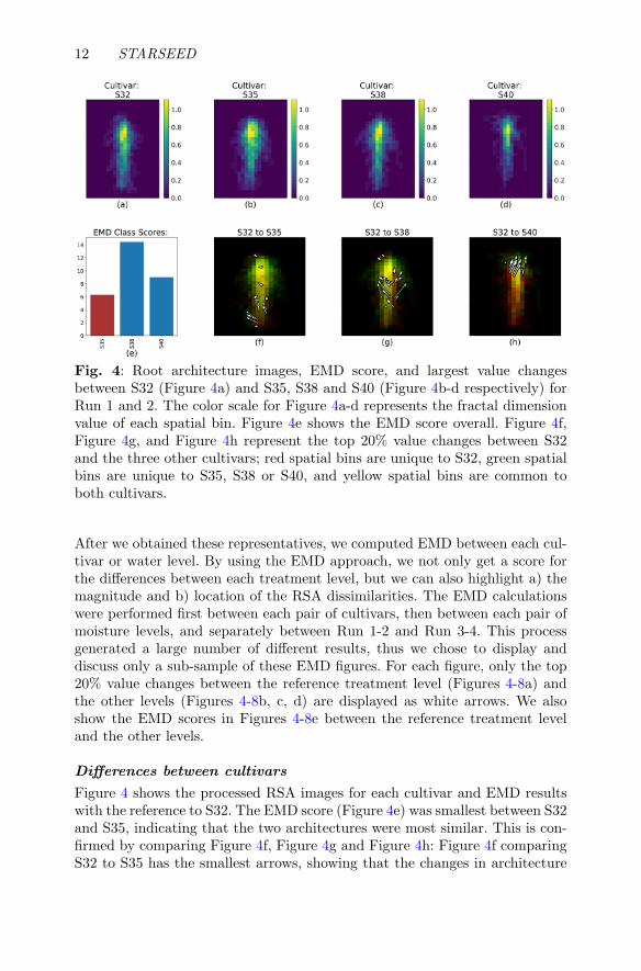
Fig. 4: Root architecture images, EMD score, and largest value changesbetween S32 (Figure 4a) and S35, S38 and S40 (Figure 4b-d respectively) forRun 1 and 2. The color scale for Figure 4a-d represents the fractal dimensionvalue of each spatial bin. Figure 4e shows the EMD score overall. Figure 4f,Figure 4g, and Figure 4h represent the top 20% value changes between S32and the three other cultivars; red spatial bins are unique to S32, green spatialbins are unique to S35, S38 or S40, and yellow spatial bins are common toboth cultivars.

After we obtained these representatives, we computed EMD between each cul-tivar or water level. By using the EMD approach, we not only get a score forthe differences between each treatment level, but we can also highlight a) themagnitude and b) location of the RSA dissimilarities. The EMD calculationswere performed first between each pair of cultivars, then between each pair ofmoisture levels, and separately between Run 1-2 and Run 3-4. This processgenerated a large number of different results, thus we chose to display anddiscuss only a sub-sample of these EMD figures. For each figure, only the top20% value changes between the reference treatment level (Figures 4-8a) andthe other levels (Figures 4-8b, c, d) are displayed as white arrows. We alsoshow the EMD scores in Figures 4-8e between the reference treatment leveland the other levels.

Differences between cultivars

Figure 4 shows the processed RSA images for each cultivar and EMD resultswith the reference to S32. The EMD score (Figure 4e) was smallest between S32and S35, indicating that the two architectures were most similar. This is con-firmed by comparing Figure 4f, Figure 4g and Figure 4h: Figure 4f comparingS32 to S35 has the smallest arrows, showing that the changes in architecture

STARSEED 13

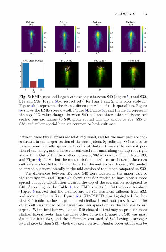
Fig. 5: EMD score and largest value changes between S40 (Figure 5a) and S32,S35 and S38 (Figure 5b-d respectively) for Run 1 and 2. The color scale forFigure 5b-d represents the fractal dimension value of each spatial bin. Figure5e shows the EMD score overall. Figure 5f, Figure 5g, and Figure 5h representthe top 20% value changes between S40 and the three other cultivars; redspatial bins are unique to S40, green spatial bins are unique to S32, S35 orS38, and yellow spatial bins are common to both cultivars.

between these two cultivars are relatively small, and for the most part are con-centrated in the deeper section of the root system. Specifically, S35 seemed tohave a more laterally spread out root distribution towards the deepest por-tion of the image, and a more concentrated root mass along the tap root rightabove that. Out of the three other cultivars, S32 was most different from S38,and Figure 4g shows that the most variation in architecture between these twocultivars was located in the middle part of the root system. Indeed, S38 tendedto spread out more laterally in the mid-section of the image compared to S32.

The differences between S32 and S40 were located in the upper part ofthe root system, and Figure 4h shows that S32 tended to have more a morespread out root distribution towards the top of the soil surface compared toS40. According to the Table 1, the EMD results for S40 without fertilizer(Figure 5 showed that the architecture for S40 was most different from S32,and most similar to S35 (Figure 5e). STARSEED also highlighted the factthat S40 tended to have a pronounced shallow lateral root growth, while theother cultivars tended to be denser and less spread out in the very shallowestdepth. When fertilizer was added, S40 showed a tendency to produce moreshallow lateral roots than the three other cultivars (Figure 6). S40 was mostdissimilar from S32, and the differences consisted of S40 having a strongerlateral growth than S32, which was more vertical. Similar observations can be

14 STARSEED

Fig. 6: Root architecture images, EMD score and largest value changesbetween S40 (Figure 6a) and S32, S35 and S38 (Figure 6b-d respectively) forRun 3 and 4. The color scale for Figure 6b-d represents the percentage of rootpixels in each spatial bin. Figure 6e shows the EMD score overall. Figure 6f,Figure 6g, and Figure 6h represent the top 20% value changes between S40and the three other cultivars; red spatial bins are unique to S40, green spatialbins are unique to S32, S35 or S38, and yellow spatial bins are common toboth cultivars.

made between S40 and S35, though S35 seemed to have more lateral growththan S32. With S38 the differences between the two architectures were notfocused on one specific area and tended to be smaller overall, indicative of amore similar architecture also evidenced by the low EMD score between S40and S38 (Figure 6e).

Differences between moisture levels

For Runs 1 and 2, when considering water levels, the root architectures wereoverall very similar as shown in Table 1. The architecture that was most dis-tinguished from the others was that of the 80% moisture treatment (Figure7). It was overall most different from 100%, and was closest to 120% and the60% treatment architecture (Figure 7e). Specifically, the 80% treatment hada visibly denser central region than the three other moisture levels (Figure 7athrough Figure 7d). This is reflected more clearly in Figure 7f through h: the80% treatment showed a more concentrated root distribution closer to the topof the root system compared to the other treatments, and so the arrows tendto point toward the upper center of the root system. The fertilizer added inRun 3 and 4 substantially changed the plant development curve from sigmoidalto exponential. The architecture for the 120% moisture level was appearedextremely different from the other moisture levels (Table 2, Figure 8). The

STARSEED 15

Fig. 7: Root architecture images, EMD score and largest value changesbetween 80% (Figure 7a) and 60%, 100% and 120% (Figure 7b-d respectively)for Run 1 and 2. The color scale for Figure 7b-d represents the percentage ofroot pixels in each spatial bin. Figure 7e shows the EMD score overall. Figure7f, Figure 7g, and Figure 7h represent the top 20% value changes between80% and the three other mositure levels; red spatial bins are unique to 80%,green spatial bins are unique to 60%, 100% or 120%, and yellow spatial binsare common to both water levels.

roots barely grew beyond the flooded layer of soil, and tended to spread outlaterally to a greater extent than in the other soil moisture conditions. Theroots for 120% also tended to be more dense right above the flooded layer ofsoil, as evidenced by higher color scale value in Figure 8a.

4 Discussion

4.1 Avoidance vs Tolerance in waterlogged soil conditions

When looking at the EMD results, one interesting observation is that the threefeatures that were considered (i.e., % root pixels, fractal dimension and lacu-narity) had very similar discriminating power between cultivars and betweenmoisture levels (Table 1, Table 2) though the ANOVA/Tukey HSD test showedthat % root pixels tended to be a better feature than fractal dimension andlacunarity. Both fractal dimension and lacunarity have been used successfullyin RSA analysis (Li et al, 2020; Walk et al, 2004). However, the main differ-ences between these previous studies and the current one is that in this studythese features were not calculated across the entire image but for each spatialbin.

16 STARSEED

Fig. 8: Root architecture images, EMD score and largest value changesbetween 120% (Figures 8a) and 60%, 80% and 100% (Figures 8b-d respectively)for Run 3 and 4. The color scale for Figures 8b-d represents the percentage ofroot pixels in each spatial bin. Figures 8e shows the EMD score overall. Figures8f, Figures 8g and Figures 8h represent the the top 20% value changes between120% and the three other moisture levels; red spatial bins are unique to 120%,green spatial bins are unique to 60%, 80% or 100%, and yellow spatial binsare common to both water levels.

We also calculated the fractal dimension and lacunarity values for wholeimages, but we observed limited differences among treatments for the CH index(e.g., S32 = 0.06 and S38 = 0.03 for Runs 3 and 4 with fractal dimension).By using these texture features to describe the individual regions of an image,we improved the RSA characterization and comparisons for each treatment.Results from Tables 1 and 2 indicate that for future similar work, % rootpixels, an easily calculated parameter, should be preferentially used ratherthan fractal dimension and lacunarity.

More specifically, the results for Runs 1-2 and Runs 3-4 (Table 1 and 2)indicate that without fertilizer, cultivar is the dominant driver of root architec-ture, and that water only plays a minimal role. This can be seen in the highestCH index score on average across all cultivars compared with the averages forwater level (Table 1). S32 was the cultivar with the most distinct architecture,and through Figure 4, we are able to pinpoint what made this architecturedifferent from the others such as having most changes in the deeper sectionof the root architecture through a less concentrated root mass along the rightof the tap root (S35), the most variation in the lateral spread in the middlepart of the root system (S38), and the most difference in the upper part of the

STARSEED 17

root system by a more spread out root distribution towards the top of the soilsurface (S40).

The situation is reversed when fertilizer is added, and water level becomesthe factor with the biggest impact on root architecture, as evidenced by themuch higher CH index value for moisture level. This high score is actuallydriven by a single treatment, 120% moisture level, which had a very differentarchitecture compared to the other soil moisture treatment (Figure 8). Theroots seemed to not be able to grow much into the flooded layer of soil, andtended to grow laterally more so than in the other treatments. This verydistinct RSA in flooded conditions when fertility is adequate in Run 3 and 4contrasts strongly with that of Run 1 and 2. Sesame is known to be highlysensitive to waterlogged soil (Sarkar et al, 2016), and can activate a varietyof morpho-anatomical and physiological responses to cope with flooding stress(Wei et al, 2013). Here, we can highlight two different morpho-anatomicalstrategies employed by the crop depending on the soil fertility status. Withoutadequate nutrient availability, the crop seems to opt for a tolerance strategyto flooding, developing roots into the saturated soil (Figure 7). We can assumethat this apparent tolerance strategy is accompanied but other changes notcaptured in this study such as the formation of aerenchyma and changes in theenzymatic activities (Wei et al, 2013). When there are enough nutrients in thesoil however, the plants seemed to adopt an avoidance strategy, and did notgrow roots down into the waterlogged soil, but tended to proliferate laterally(Figure 8). These observations being constant across cultivars, we can thusconclude that fertility conditions the response of sesame early RSA to floodingstress.

4.2 Validity of the EMD Method

Although of interest in estimating early root vigor and biomass, it is clear herethat only considering TRL does not provide any insight on RSA. Increasing ourknowledge and understanding of root architectural development in responseto environmental stresses is of capital importance for global agricultural pro-duction, and has been defined as the pillar of the Second Green Revolution(Lynch, 2007). Many methods are now available to observe RSA, yet someof the more advanced techniques such as CT imaging remain expensive andimpractical, underlining the need for improved trans-disciplinary phenotypingapproaches that can capture and quantify the complexity of RSA (Atkinsonet al, 2019; Wu et al, 2018; Zhu et al, 2011).

Our proposed STARSEED method could be the answer to some of theseissues. It provides a fast, reproducible, quantitative, and spatially explicit char-acterization of RSA, also allowing for comparisons between root systems. Avaluable aspect of the analysis is the introduction of the EMD class score, whichsummarizes all of the differences between two RSAs down to a single numberwhich can be compared between these RSAs. The EMD scores also providean interpretable measure that quantifies the visual observations between theroot structures. EMD, combined with the CH index, can thus be used to very

18 STARSEED

quickly know which treatment lead to the most distinct RSA, and the degreeto which these RSAs relate to one another globally.

The actual spatial EMD result (i.e., Figures 4 through 8) can then belooked at to further elucidate specific spatial differences between RSAs. Tothe best of the authors’ knowledge, this is the first time EMD has been usedto characterize RSA. The method has been thoroughly validated and usedin varied fields of science, including fluid mechanics (Benamou and Brenier,2000), linguistics (Kusner et al, 2015), or, more related to the present study,image classification and comparison (Zhang et al, 2020). The CH index usedin STARSEED serves as evaluation step for the method to not only quantifywhat we observe, but also to ensure the approach captures distinct featuresto effectively group root architectures based on a shared characteristic (e.g.,cultivar, moisture treatment).

One of the most critical strengths of STARSEED and the way it is per-formed here is that it allows for the generation of an “average” root architecturevisual representation as shown in Figures 4 through 8a through d. Indeed, bytaking the overlap of all images within one treatment, partitioning the imageinto local regions, and calculating a feature value for each spatial bin, we cangenerate a meaningful and visually explicit “average” architecture that reflectsdifferences between genotypes or environmental conditions. Recent studieshave attempted to either develop new techniques to directly measure RSA(Armengaud et al, 2009), find a way to accurately represent average RSAscorresponding to specific growing conditions (Shahzad et al, 2018), and manymore studies have developed or refined root architecture development models(Tron et al, 2015; Postma et al, 2017; Zhao et al, 2017; Pages et al, 2020). Onestudy in particular created similar 2D heat maps of “root frequency” observedon the four transparent surfaces of rhizoboxes but did not perform a spatiallyexplicit analysis to the level of STARSEED (Jørgensen et al, 2014).

4.3 Going beyond the 2D images of rhizoboxes

Given the rhizobox set up of this study and the use of flatbed scanners forroot images acquisition, the observations are confined in 2D when root sys-tems always exist in 3D spaces. Imaging and characterizing a whole RSA in 3Din situ or even in vitro is usually low throughput and expensive if not nearlyimpossible. Most scientists thus resort to using models in lieu of direct obser-vations, as previously mentioned. One of the main difficulty of using these 3DRSA models is correct parameterization, which is crucial to the accuracy andvalidity of a model’s prediction (Schnepf et al, 2018). Recent work has shownthat 2D measurements of root systems could be used to adequately inform theparameters for 3D models (in wheat (Landl et al, 2018)). It is thus a reasonablehypothesis to say that the current EMD results could be further refined andsubsequently used to generate and interpret such 3D models. There is poten-tial to go even further and directly use EMD on 3D data (Salti et al, 2014),although the issue of acquiring such data still remains.

STARSEED 19

Combining the average EMD visual maps with new root architecture quan-tification techniques (Wu and Guo, 2014) could really boost our understandingof RSA plasticity. This would allow for both global (i.e., EMD scores) and local(i.e., magnitude and direction of changes) comparisons between genotypes andenvironmental conditions. Additionally, combining our understanding of RSAplasticity derived from the EMD visual maps along with molecular and geneticwork would most probably be of critical importance to breeders.

5 Conclusion

In this paper, we presented STARSEED, an approach to characterize rootarchitecture from 2D images. Qualitative and quantitative analysis demon-strate the effectiveness of the proposed method. STARSEED successfullyincorporated spatial and texture information to describe root architectures atboth global and local contexts. The method is explainable and provides clearconnections to biological aspects of each root image. STARSEED also allowsfor aggregating individual architectures to assess and average response for eachenvironmental condition and genotype. Future work includes clustering basedon root architecture (i.e., using the pairwise EMD matrix for relational clus-tering), applying our general framework over time to characterize how RSAdevelops in various conditions, along with scaling up to 3D characterization.

Declarations

Funding This material is based upon work supported by the National ScienceFoundation Graduate Research Fellowship under Grant No. DGE-1842473.

Conflict of interest/Competing interests The authors have no conflictsof interest to declare that are relevant to the content of this article.

Ethics approval Not applicable

Consent to participate Not applicable

Consent for publication Not applicable

Availability of data and materials The raw and binarized root imagesfor our experiments are publicly available: https://github.com/GatorSense/STARSEED/tree/master/Data.

Code availability The code for our experiments are publicly available:https://github.com/GatorSense/STARSEED.

Authors’ contributions Joshua Peeples, Weihuang Xu, Romain Gloaguen,Diane Rowland, and Alina Zare planned and designed the research. JoshuaPeeples, Weihuang Xu, and Romain Gloaguen collected data, conducted

20 STARSEED

experiments, and performed analysis. Joshua Peeples, Weihuang Xu, andRomain Gloagen wrote the manuscript. Diane Rowland, Alina Zare, andZachary Brym reviewed and edited the manuscript. All authors read andapproved the final manuscript.

References

Adadi A, Berrada M (2018) Peeking inside the black-box: A survey onexplainable artificial intelligence (xai). IEEE Access 6:52,138–52,160

Armengaud P, Zambaux K, Hills A, et al (2009) Ez-rhizo: integrated softwarefor the fast and accurate measurement of root system architecture. ThePlant Journal 57(5):945–956

Atkinson JA, Pound MP, Bennett MJ, et al (2019) Uncovering the hiddenhalf of plants using new advances in root phenotyping. Current opinion inbiotechnology 55:1–8

Becht E, McInnes L, Healy J, et al (2019) Dimensionality reduction forvisualizing single-cell data using umap. Nature biotechnology 37(1):38–44

Benamou JD, Brenier Y (2000) A computational fluid mechanics solutionto the monge-kantorovich mass transfer problem. Numerische Mathematik84(3):375–393

Calinski T, Harabasz J (1974) A dendrite method for cluster analysis.Communications in Statistics-theory and Methods 3(1):1–27

Chung YS, Lee U, Heo S, et al (2020) Image-based machine learning charac-terizes root nodule in soybean exposed to silicon. Frontiers in plant science11

Cula OG, Dana KJ (2001) Compact representation of bidirectional texturefunctions. In: Proceedings of the 2001 IEEE Computer Society Conferenceon Computer Vision and Pattern Recognition. CVPR 2001, IEEE, pp I–I

Gulrajani I, Ahmed F, Arjovsky M, et al (2017) Improved training of wasser-stein gans. In: Proceedings of the 31st International Conference on NeuralInformation Processing Systems, pp 5769–5779

Gunning D (2017) Explainable artificial intelligence (xai). Defense AdvancedResearch Projects Agency (DARPA), nd Web

Hitchcock FL (1941) The distribution of a product from several sources tonumerous localities. Journal of mathematics and physics 20(1-4):224–230

STARSEED 21

Jørgensen L, Dresbøll DB, Thorup-Kristensen K (2014) Spatial root distribu-tion of plants growing in vertical media for use in living walls. Plant andsoil 380(1):231–248

Keller JM, Chen S, Crownover RM (1989) Texture description and segmen-tation through fractal geometry. Computer Vision, Graphics, and imageprocessing 45(2):150–166

Kruskal JB (1964) Multidimensional scaling by optimizing goodness of fit toa nonmetric hypothesis. Psychometrika 29(1):1–27

Kusner M, Sun Y, Kolkin N, et al (2015) From word embeddings to documentdistances. In: International conference on machine learning, PMLR, pp 957–966

Landl M, Schnepf A, Vanderborght J, et al (2018) Measuring root system traitsof wheat in 2d images to parameterize 3d root architecture models. Plantand soil 425(1):457–477

Li S, Wan L, Nie Z, et al (2020) Fractal and topological analyses and antiox-idant defense systems of alfalfa (medicago sativa l.) root system underdrought and rehydration regimes. Agronomy 10(6):805

Lynch JP (2007) Roots of the second green revolution. Australian Journal ofBotany 55(5):493–512

Maaten Lvd, Hinton G (2008) Visualizing data using t-sne. Journal of machinelearning research 9(Nov):2579–2605

Mandelbrot B (1967) How long is the coast of britain? statistical self-similarityand fractional dimension. science 156(3775):636–638

Mandelbrot BB, Mandelbrot BB (1982) The fractal geometry of nature, vol 1.WH freeman New York

Mandelbrot BB, Van Ness JW (1968) Fractional brownian motions, fractionalnoises and applications. SIAM review 10(4):422–437

Oza NC, Tumer K (2001) Input decimation ensembles: Decorrelation throughdimensionality reduction. In: Kittler J, Roli F (eds) Multiple ClassifierSystems. Springer Berlin Heidelberg, Berlin, Heidelberg, pp 238–247

Pages L, Pointurier O, Moreau D, et al (2020) Metamodelling a 3d architecturalroot-system model to provide a simple model based on key processes andspecies functional groups. Plant and Soil pp 1–21

Pierret A, Gonkhamdee S, Jourdan C, et al (2013) Ij rhizo: an open-sourcesoftware to measure scanned images of root samples. Plant and soil

22 STARSEED

373(1):531–539

Plotnick RE, Gardner RH, O’Neill RV (1993) Lacunarity indices as measuresof landscape texture. Landscape ecology 8(3):201–211

Postma JA, Kuppe C, Owen MR, et al (2017) Opensimroot: widening the scopeand application of root architectural models. New Phytologist 215(3):1274–1286

Pound MP, Atkinson JA, Townsend AJ, et al (2017) Deep machine learn-ing provides state-of-the-art performance in image-based plant phenotyping.Gigascience 6(10):gix083

Rubner Y, Guibas LJ, Tomasi C (1997) The earth mover’s distance, multi-dimensional scaling, and color-based image retrieval. In: Proceedings of theARPA image understanding workshop, p 668

Rubner Y, Tomasi C, Guibas LJ (1998) A metric for distributions with appli-cations to image databases. In: Sixth International Conference on ComputerVision (IEEE Cat. No. 98CH36271), IEEE, pp 59–66

Salti S, Tombari F, Di Stefano L (2014) Shot: Unique signatures of his-tograms for surface and texture description. Computer Vision and ImageUnderstanding 125:251–264

Sarkar N, Chaudhuri BB (1992) An efficient approach to estimate fractaldimension of textural images. Pattern recognition 25(9):1035–1041

Sarkar P, Khatun A, Singha A (2016) Effect of duration of water-logging oncrop stand and yield of sesame. International Journal of Innovation andApplied Studies 14(1):1

Schnepf A, Huber K, Landl M, et al (2018) Statistical characterization of theroot system architecture model crootbox. Vadose zone journal 17(1):1–11

Shahzad Z, Kellermeier F, Armstrong EM, et al (2018) Ez-root-vis: a soft-ware pipeline for the rapid analysis and visual reconstruction of root systemarchitecture. Plant physiology 177(4):1368–1381

TATSUMI J, YAMAUCHI A, KONO Y (1989) Fractal analysis of plant rootsystems. Annals of Botany 64(5):499–503

Tron S, Bodner G, Laio F, et al (2015) Can diversity in root architectureexplain plant water use efficiency? a modeling study. Ecological modelling312:200–210

Tuceryan M, Jain AK (1993) Texture analysis. Handbook of pattern recogni-tion and computer vision pp 235–276

STARSEED 23

Voss RF (1991) Random fractals: characterization and measurement. In:Scaling phenomena in disordered systems. Springer, p 1–11

Walk TC, Van Erp E, Lynch JP (2004) Modelling applicability of frac-tal analysis to efficiency of soil exploration by roots. Annals of Botany94(1):119–128

Wang H, Siopongco J, Wade LJ, et al (2009) Fractal analysis on root systemsof rice plants in response to drought stress. Environmental and ExperimentalBotany 65(2-3):338–344

Wei W, Li D, Wang L, et al (2013) Morpho-anatomical and physiologicalresponses to waterlogging of sesame (sesamum indicum l.). Plant science208:102–111

Wu J, Guo Y (2014) An integrated method for quantifying root architectureof field-grown maize. Annals of botany 114(4):841–851

Wu Q, Wu J, Zheng B, et al (2018) Optimizing soil-coring strategies to quantifyroot-length-density distribution in field-grown maize: virtual coring trialsusing 3-d root architecture models. Annals of botany 121(5):809–819

Xu W, Yu G, Zare A, et al (2020) Overcoming small minirhizotrondatasets using transfer learning. Computers and Electronics in Agriculture175:105,466

Yasrab R, Atkinson JA, Wells DM, et al (2019) Rootnav 2.0: Deep learningfor automatic navigation of complex plant root architectures. GigaScience8(11):giz123

Yu G, Zare A, Sheng H, et al (2020) Root identification in minirhizotronimagery with multiple instance learning. Machine Vision and Applications31(6):1–13

Zhang C, Cai Y, Lin G, et al (2020) Deepemd: Few-shot image classificationwith differentiable earth mover’s distance and structured classifiers. In: Pro-ceedings of the IEEE/CVF Conference on Computer Vision and PatternRecognition, pp 12,203–12,213

Zhao J, Bodner G, Rewald B, et al (2017) Root architecture simulationimproves the inference from seedling root phenotyping towards mature rootsystems. Journal of experimental botany 68(5):965–982

Zhu J, Ingram PA, Benfey PN, et al (2011) From lab to field, new approachesto phenotyping root system architecture. Current opinion in plant biology14(3):310–317