ORIGINAL PAPER

Spatial and temporal dynamics of Pai forest vegetation in Pakistanassessed by RS and GIS

A. A. Siyal1,2 • A. G. Siyal2 • R. B. Mahar1

Received: 18 September 2014 / Accepted: 6 February 2016

� Northeast Forestry University and Springer-Verlag Berlin Heidelberg 2016

Abstract Pai, an arid forest in Sindh Province of Pakistan,

is important for the environmental, social, economic

development and conservation of ecosystems of the pro-

vince. Considering the significance of the forest for Sindh

and the calls from the local population for its deforestation,

we quantified the spatial and temporal variation in the

vegetation of the forest and land surface temperature (LST)

using optical and thermal Landsat satellite data. Our

analysis of temporal (1987–2014) images with ArcGIS

10.1 revealed that the dense forest area was greatest at

725 ha (37 % of the total forest area) during 2013 while it

was smallest at 217 ha (11 %) in 1992. The sparse forest

area peaked during 1987 at 1115 ha (58 %) under shrubs

whereas it was smallest at 840 ha (43 %) in 1992, and the

maximum deforestation of Pai forest occurred during 1992.

Spatial change in vegetation over a period of about

27 years (1987–2014) revealed that vegetation increased

on an area of 735 ha (37 %), decreased on 427 ha (22 %),

and there was no change on 808 ha (41 %) of the forest.

Variation in temperature between shaded (dense forest) and

unshaded areas (bare land) of the forest was from 6 to

10 �C. While the temperature difference between areas

with sparse forest and bare land ranged from 4 to 6 �C. An

inverse relationship between LST and NDVI of Pai forest

with coefficients of determination of 0.944 and 0.917 was

observed when NDVI was plotted against minimum and

maximum LST, respectively. The vegetation in the forest

increased with time and the areas of more dense Pai forest

supported lower surface temperature and thus air

temperature.

Keywords Landsat � Arid forest � NDVI � Deforestation �Ecosystem � Land surface temperature (LST)

Introduction

Forests not only provide livelihood to about one billion

people (UNEP 2011; Sunderland et al. 2013) but also

provide employment directly or indirectly to more than one

hundred million people around the globe (UNEP 2011).

Forests protect environment through soil conservation,

watershed management, and provide protection against

floods and landslides. Forests have an important impact on

local as well as global environment and climate change

(Xiao et al. 2004). Temporal changes in forest land cover

can result in a wide variety of ecological impacts, including

changes in productivity, composition, nutrient dynamics,

species diversity, and increased atmospheric carbon diox-

ide (Braswell et al. 2003).

Measuring, mapping and classifying forests is important

for monitoring spatial and temporal variation in vegetation

and for planning and implementation of forest restoration

programs (Rikimaru 1999). Traditional methods of map-

ping and categorizing forests through field surveys, litera-

ture reviews, map interpretation and secondary data

analysis are time consuming, laborious, and uneconomical.

Therefore, Remote Sensing and GIS tools are often used

The online version is available at http://www.springerlink.com

Corresponding editor: Yu Lei.

& A. A. Siyal

siyal@yahoo.com

1 U.S.-Pakistan Center for Advanced Studies in Water

(USPCAS-W), Mehran University of Engineering and

Technology, Jamshoro, Pakistan

2 Department of Land and Water Management, Sindh

Agriculture University, Tandojam, Pakistan

123

J. For. Res.

DOI 10.1007/s11676-016-0327-x

for mapping, monitoring and analyzing forest vegetation as

these tools are economical and rapid (Kumar 2010).

Acquiring high spatial resolution satellite imagery is often

expensive and cost-prohibitive. In contrast, Google Earth�

(GE) is a free source of high resolution satellite imagery

(Madin et al. 2011; Hughes et al. 2011; Pringle 2010) but

its applications are limited by inadequate temporal avail-

ability of imagery and low spectral resolution and number

of spectral bands (Potere 2008; McInnes et al. 2011).

Hence, Landsat imagery is widely used for monitoring

global surface change as it is a free multispectral and

medium spatial resolution resource of imagery (Goward

et al. 2006; Masek et al. 2008; Wulder et al. 2008; Xie et al.

2008; Bhandari et al. 2012). The diurnal land surface

temperature (LST) derived from thermal infrared (TIR)

bands is reported to be closely related to the density of the

forest canopy (Nemani and Running 1997). Pongratz et al.

(2006) confirmed that increase in LST occurs in areas with

lower forest cover compared with dense forest. Yang et al.

(2007) observed a good agreement with coefficient of

determination of R2 = 0.80 and RMSE = 0.7 �C between

predicted and observed air-surface temperature profile in

mixed forest. Wickham et al. (2012) reported that forest

surface temperatures were cooler than cropland surface

temperatures. Thus, day LST can be used to detect changes

in the forest cover (van Leeuwen et al. 2011).

Pai forest, one of the major forests of Sindh, Pakistan is

reported to be endangered due to natural factors such as

chronic water shortage, soil salinization, threats from land

grabbers and lumber mafia, and deforestation due to cutting

of trees by nearby villagers (WWF 2008). It is claimed by

local people that trees are cut from an area of about 200 ha

and the land is then brought under cultivation for crops.

These threats are countered by calls from civil society to

prevent deforestation and conserve the forest. There is a

need to study the temporal and spatial change in the veg-

etation of the forest in order to analyze threats to the forest

as claimed by people. Our study was thus conducted using

temporal Landsat optical data to quantify the spatial and

temporal variation in the vegetation of the forest. Spatial

variation in LST during winter (January), spring (March),

summer (June) and autumn (October) was determined from

Landsat TIR data for the year 2013–2014 only.

Materials and methods

Study area

Pakistan has about 4.57 million hectares of forests, which

is equivalent to 5.2 % of the total geographical area (GoP

2003). This is low compared to the global average of 30 %

(FAO 2001) but the climate of Pakistan is predominantly

arid and largely unsuited to forest development. The total

riverine area in Sindh, Pakistan is 0.855 million ha which is

confined between flood protective embankments on both

sides of the main stream of the river Indus (Panhwar 2002).

The riverine forests in Sindh are mostly on rich alluvial

soils that support trees such as Prosopis juliflora (Babol),

Acacia nilotica (Kikar), Populus euphratica (Bahan), Ta-

marix aphylla and Tamarix dioica (Lai), Dalbergia sissoo

(Shesham), Prosopis cineraria (Kandi), and Azadirachta

indica (Neem). These forests are the major sources of

timber, firewood and fodder for livestock (Mughal 2010).

Pai forest is considered to be one of the important forest

of Sindh province and covers an area of 1977 ha. It is

surrounded by vast fertile cultivated lands (Qureshi and

Bhatti 2010; Faruqi 2011). WWF (2008) reported that

during 2008, about 1502 ha (76 %) were under tree cover

while the remaining 468 ha (23.7 %) were either cultivated

or were bare land with salty patches. The forest is located

in arid area with mean annual rainfall of about 150 mm and

maximum surface evaporation rates of about

9–10 mm day-1 during May and June.

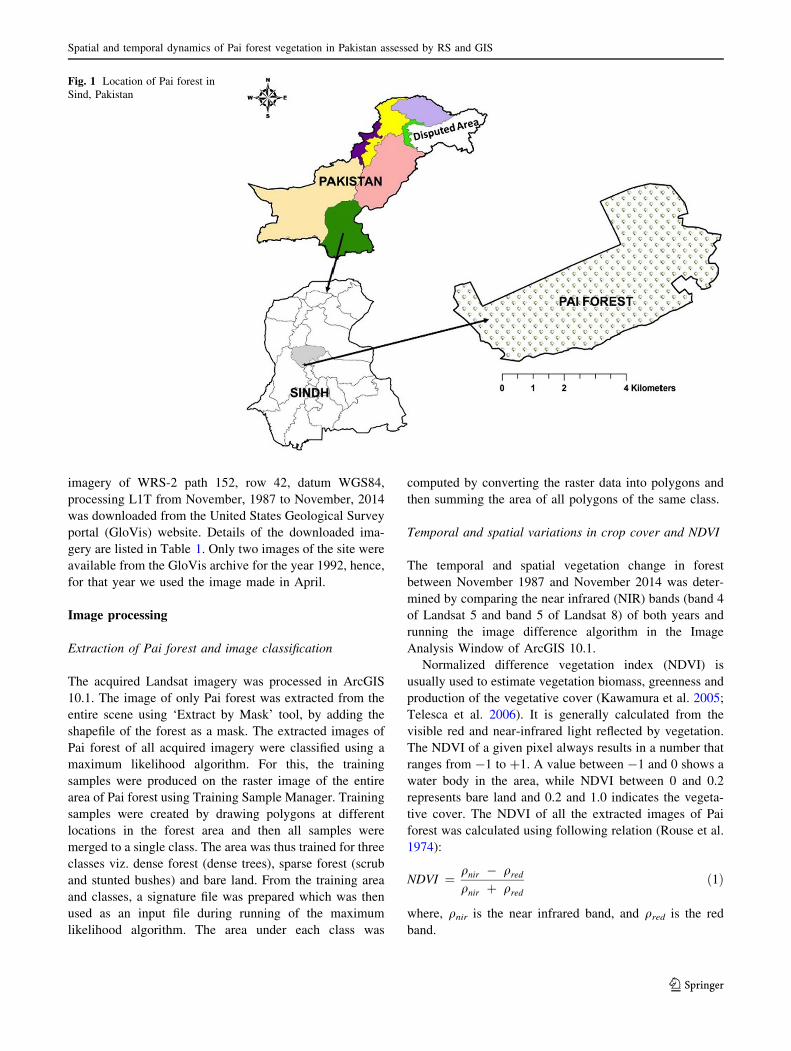
The forest is situated in Shaheed Benazirabad, a central

district of Sindh, near Sakrand town on the left bank of the

river Indus between longitudes 68�1202000 and 68�1700400Eand latitudes 26�0405000 and 26�0704000N at 30 m above

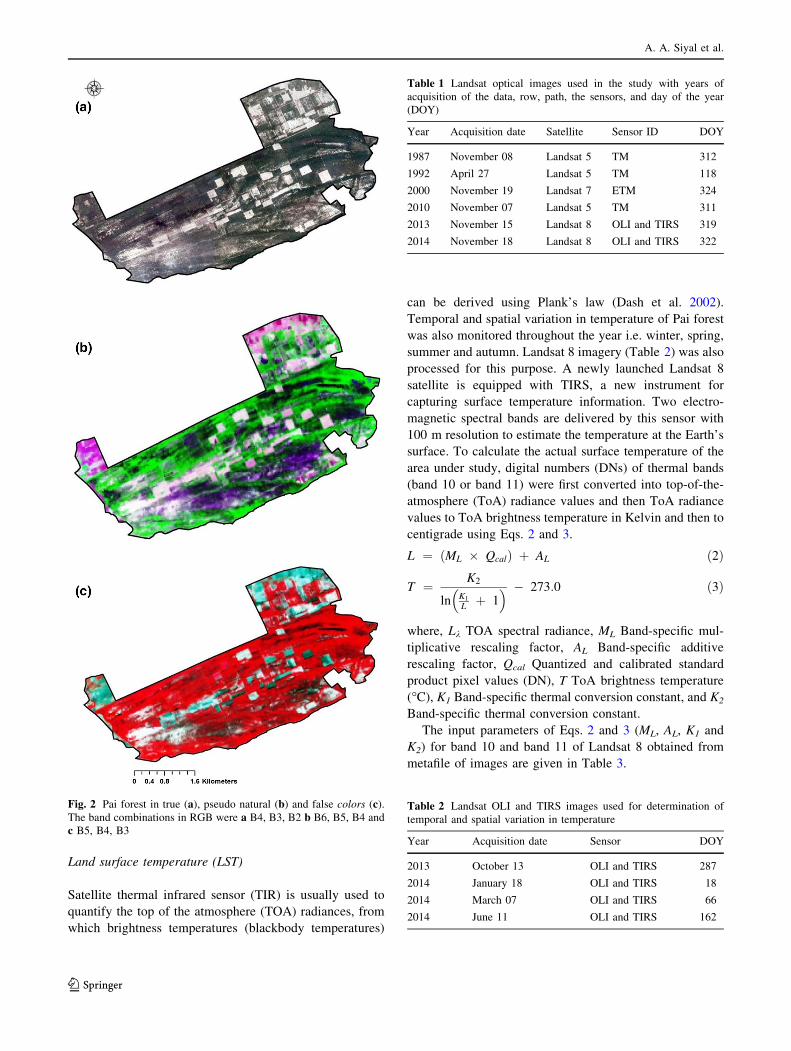
mean sea level (Fig. 1). The Pai forest in true color, pseudo

natural color, and false color is shown in Fig. 2. The study

area is mainly covered by vegetation (Fig. 2c). Areas

covered by isolated bushes are shown in purple color in

Fig. 2b, agricultural land is shown in magenta color in

Fig. 2b, and bare land is shown in white color in Fig. 2a.

Pai forest was a riverine forest until its source of irri-

gation was cut off from the river Indus due to construction

of flood protection bunds along the Indus river banks

during the era of British rule. It is now a canal irrigated

forest, being irrigated by the Rahib Shah distributary, a

branch of the Rohri Canal and by groundwater through

tube-wells installed for this purpose. The forest provides

habitat for flora and fauna including the indigenous Mes-

quite (P. juliflora), Arabic gumtree (A. nilotica), Spunge

tree (P. cineraria), Indian rosewood or Bombay Black-

wood (D. sissoo) and Hog deer, Partridges, Asiatic jackals,

Jungle cat, Porcupine, reptiles. Qureshi and Bhatti (2010)

reported total of 93 plant species in the forest. The forest

also provides livelihood to 21 villages located on the

periphery of the forest. They are dependent upon the nat-

ural products of the forest to meet their daily requirement

of food, fuel wood and earnings.

Satellite imagery

Temporal and spatial variation in vegetative cover of Pai

forest was quantified using Landsat imagery. Landsat

A. A. Siyal et al.

123

imagery of WRS-2 path 152, row 42, datum WGS84,

processing L1T from November, 1987 to November, 2014

was downloaded from the United States Geological Survey

portal (GloVis) website. Details of the downloaded ima-

gery are listed in Table 1. Only two images of the site were

available from the GloVis archive for the year 1992, hence,

for that year we used the image made in April.

Image processing

Extraction of Pai forest and image classification

The acquired Landsat imagery was processed in ArcGIS

10.1. The image of only Pai forest was extracted from the

entire scene using ‘Extract by Mask’ tool, by adding the

shapefile of the forest as a mask. The extracted images of

Pai forest of all acquired imagery were classified using a

maximum likelihood algorithm. For this, the training

samples were produced on the raster image of the entire

area of Pai forest using Training Sample Manager. Training

samples were created by drawing polygons at different

locations in the forest area and then all samples were

merged to a single class. The area was thus trained for three

classes viz. dense forest (dense trees), sparse forest (scrub

and stunted bushes) and bare land. From the training area

and classes, a signature file was prepared which was then

used as an input file during running of the maximum

likelihood algorithm. The area under each class was

computed by converting the raster data into polygons and

then summing the area of all polygons of the same class.

Temporal and spatial variations in crop cover and NDVI

The temporal and spatial vegetation change in forest

between November 1987 and November 2014 was deter-

mined by comparing the near infrared (NIR) bands (band 4

of Landsat 5 and band 5 of Landsat 8) of both years and

running the image difference algorithm in the Image

Analysis Window of ArcGIS 10.1.

Normalized difference vegetation index (NDVI) is

usually used to estimate vegetation biomass, greenness and

production of the vegetative cover (Kawamura et al. 2005;

Telesca et al. 2006). It is generally calculated from the

visible red and near-infrared light reflected by vegetation.

The NDVI of a given pixel always results in a number that

ranges from -1 to ?1. A value between -1 and 0 shows a

water body in the area, while NDVI between 0 and 0.2

represents bare land and 0.2 and 1.0 indicates the vegeta-

tive cover. The NDVI of all the extracted images of Pai

forest was calculated using following relation (Rouse et al.

1974):

NDVI ¼ qnir � qredqnir þ qred

ð1Þ

where, qnir is the near infrared band, and qred is the red

band.

Fig. 1 Location of Pai forest in

Sind, Pakistan

Spatial and temporal dynamics of Pai forest vegetation in Pakistan assessed by RS and GIS

123

Land surface temperature (LST)

Satellite thermal infrared sensor (TIR) is usually used to

quantify the top of the atmosphere (TOA) radiances, from

which brightness temperatures (blackbody temperatures)

can be derived using Plank’s law (Dash et al. 2002).

Temporal and spatial variation in temperature of Pai forest

was also monitored throughout the year i.e. winter, spring,

summer and autumn. Landsat 8 imagery (Table 2) was also

processed for this purpose. A newly launched Landsat 8

satellite is equipped with TIRS, a new instrument for

capturing surface temperature information. Two electro-

magnetic spectral bands are delivered by this sensor with

100 m resolution to estimate the temperature at the Earth’s

surface. To calculate the actual surface temperature of the

area under study, digital numbers (DNs) of thermal bands

(band 10 or band 11) were first converted into top-of-the-

atmosphere (ToA) radiance values and then ToA radiance

values to ToA brightness temperature in Kelvin and then to

centigrade using Eqs. 2 and 3.

L ¼ ML � Qcalð Þ þ AL ð2Þ

T ¼ K2

ln K1

Lþ 1

� � � 273:0 ð3Þ

where, Lk TOA spectral radiance, ML Band-specific mul-

tiplicative rescaling factor, AL Band-specific additive

rescaling factor, Qcal Quantized and calibrated standard

product pixel values (DN), T ToA brightness temperature

(�C), K1 Band-specific thermal conversion constant, and K2

Band-specific thermal conversion constant.

The input parameters of Eqs. 2 and 3 (ML, AL, K1 and

K2) for band 10 and band 11 of Landsat 8 obtained from

metafile of images are given in Table 3.

Fig. 2 Pai forest in true (a), pseudo natural (b) and false colors (c).The band combinations in RGB were a B4, B3, B2 b B6, B5, B4 and

c B5, B4, B3

Table 1 Landsat optical images used in the study with years of

acquisition of the data, row, path, the sensors, and day of the year

(DOY)

Year Acquisition date Satellite Sensor ID DOY

1987 November 08 Landsat 5 TM 312

1992 April 27 Landsat 5 TM 118

2000 November 19 Landsat 7 ETM 324

2010 November 07 Landsat 5 TM 311

2013 November 15 Landsat 8 OLI and TIRS 319

2014 November 18 Landsat 8 OLI and TIRS 322

Table 2 Landsat OLI and TIRS images used for determination of

temporal and spatial variation in temperature

Year Acquisition date Sensor DOY

2013 October 13 OLI and TIRS 287

2014 January 18 OLI and TIRS 18

2014 March 07 OLI and TIRS 66

2014 June 11 OLI and TIRS 162

A. A. Siyal et al.

123

By extracting the LST values from randomly selected

points of ToA brightness temperature raster image, the

spatial variation of LST under different land use classes

(bare land, sparse forest and dense forest) was determined.

A study conducted by Li et al. (2008) to investigate the

relationship between LST and air temperature revealed that

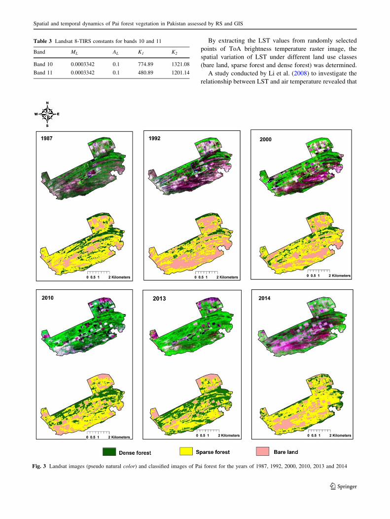
Table 3 Landsat 8-TIRS constants for bands 10 and 11

Band ML AL K1 K2

Band 10 0.0003342 0.1 774.89 1321.08

Band 11 0.0003342 0.1 480.89 1201.14

Fig. 3 Landsat images (pseudo natural color) and classified images of Pai forest for the years of 1987, 1992, 2000, 2010, 2013 and 2014

Spatial and temporal dynamics of Pai forest vegetation in Pakistan assessed by RS and GIS

123

differences are relatively small in areas of high temperature

but are larger in low temperature areas. They also reported

moderate to high correlations ranging from 0.73 to 0.79

between air temperature and LST. For the present study

difference between air temperature and LST was assumed

very small as Pai forest is located in hot and dry climate

region.

Results and discussion

Temporal and spatial variations in vegetative cover

Figure 3 shows the Landsat images in pseudo natural color

and classified images of Pai forest for the years 1987, 1992,

2000, 2010, 2013 and 2014. All the Landsat images of Pai

forest were classified for dense forest (pixels represent only

trees), sparse forest (mixed pixels representing both sparse

shrubs and bare land) and bare land (pixels represent only

bare land). Variation in vegetative cover of Pai forest from

1987 to 2014 showed that about 1552 ha (79 %) of forest

were covered with vegetation (trees and shrubs) in 1987.

This declined to 1057 ha (53 %) in 1992, a 26 % reduction

in vegetative cover in 5 years (Table 4). This might have

been due to illegal harvest of trees or drying of trees due to

shortage of irrigation water during that period as reported

by Siddiqui (2009). We were unable to confirm the cause of

the decrease in vegetative area in 1992 through consulta-

tion with the Forest Department Sindh. Another reason for

reduction in vegetation in 1992 might have been bias of the

satellite image as it was captured during April while the

rest of images were captured during winter. Our analysis of

an image captured during June 1992 revealed that there

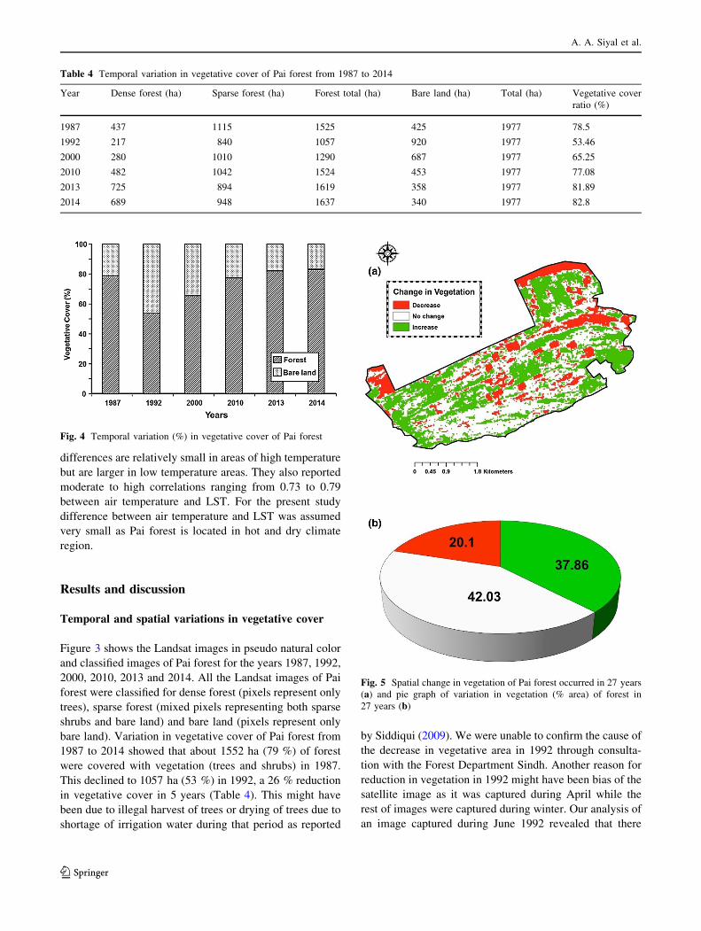
Table 4 Temporal variation in vegetative cover of Pai forest from 1987 to 2014

Year Dense forest (ha) Sparse forest (ha) Forest total (ha) Bare land (ha) Total (ha) Vegetative cover

ratio (%)

1987 437 1115 1525 425 1977 78.5

1992 217 840 1057 920 1977 53.46

2000 280 1010 1290 687 1977 65.25

2010 482 1042 1524 453 1977 77.08

2013 725 894 1619 358 1977 81.89

2014 689 948 1637 340 1977 82.8

Fig. 4 Temporal variation (%) in vegetative cover of Pai forest

Fig. 5 Spatial change in vegetation of Pai forest occurred in 27 years

(a) and pie graph of variation in vegetation (% area) of forest in

27 years (b)

A. A. Siyal et al.

123

was a non-significant difference in vegetative area repre-

sented by both images (April and June). Thus, we conclude

that the decrease in vegetation from 1987 to 1992 was not

due to the influence of the difference in season.

After 1992, the vegetated area increased to 1290 ha in

2000 (65 %), 1524 ha in 2010 (77 %), 1619 ha in 2013

(82 %), and 1637 ha in 2014 (83 %). Vegetation gradually

increased on about 467 ha (24 %) over a period of 18 years

(1992–2010) with an average annual increase in area of

26 ha (Table 4). While from 2010 to 2014, vegetation

increased on an area of about 113 ha (6 %) with an average

annual increase of 28 ha. Rapid increase in vegetation from

2010 to 2014 might be due to favorable soil moisture

conditions in forest due to above average rainfall and heavy

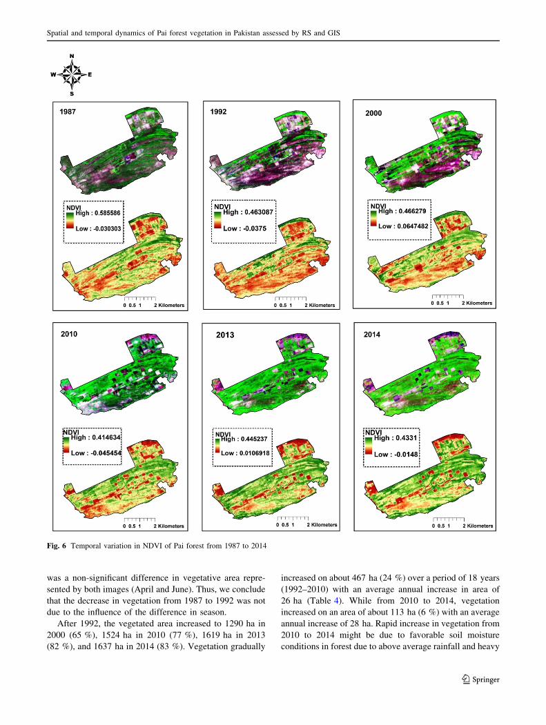
Fig. 6 Temporal variation in NDVI of Pai forest from 1987 to 2014

Spatial and temporal dynamics of Pai forest vegetation in Pakistan assessed by RS and GIS

123

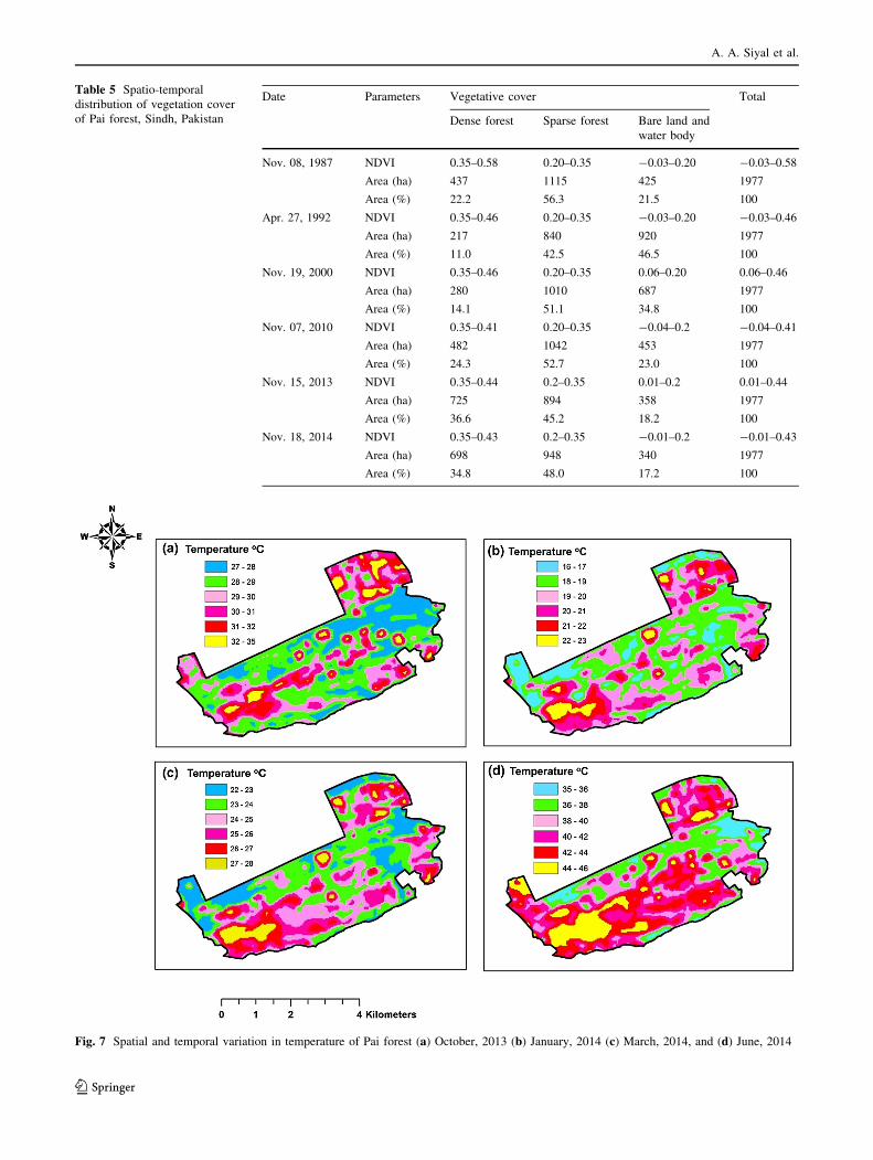
Table 5 Spatio-temporal

distribution of vegetation cover

of Pai forest, Sindh, Pakistan

Date Parameters Vegetative cover Total

Dense forest Sparse forest Bare land and

water body

Nov. 08, 1987 NDVI 0.35–0.58 0.20–0.35 -0.03–0.20 -0.03–0.58

Area (ha) 437 1115 425 1977

Area (%) 22.2 56.3 21.5 100

Apr. 27, 1992 NDVI 0.35–0.46 0.20–0.35 -0.03–0.20 -0.03–0.46

Area (ha) 217 840 920 1977

Area (%) 11.0 42.5 46.5 100

Nov. 19, 2000 NDVI 0.35–0.46 0.20–0.35 0.06–0.20 0.06–0.46

Area (ha) 280 1010 687 1977

Area (%) 14.1 51.1 34.8 100

Nov. 07, 2010 NDVI 0.35–0.41 0.20–0.35 -0.04–0.2 -0.04–0.41

Area (ha) 482 1042 453 1977

Area (%) 24.3 52.7 23.0 100

Nov. 15, 2013 NDVI 0.35–0.44 0.2–0.35 0.01–0.2 0.01–0.44

Area (ha) 725 894 358 1977

Area (%) 36.6 45.2 18.2 100

Nov. 18, 2014 NDVI 0.35–0.43 0.2–0.35 -0.01–0.2 -0.01–0.43

Area (ha) 698 948 340 1977

Area (%) 34.8 48.0 17.2 100

Fig. 7 Spatial and temporal variation in temperature of Pai forest (a) October, 2013 (b) January, 2014 (c) March, 2014, and (d) June, 2014

A. A. Siyal et al.

123

floods during 2010 and 2011 in Sindh. The temporal

variation in vegetative cover of the forest is graphically

presented in Fig. 4. Spatial variation in vegetation cover of

the forest shows that reduction in vegetation before 2010

mainly occurred at the central and southern parts along the

boundary of Pai forest but after 2010, the northeast part of

the forest was affected (Fig. 3).

The spatial change in vegetation of Pai forest occurred

over nearly 27 years from 1987 to 2014 and shows that

there was more forestation than deforestation (Fig. 5a).

This change was reflected by an increase in vegetation on

an area of 735 ha (37 %), a decline on 427 ha (22 %), and

no change on 808 ha (41 %) of the forest (Fig. 5b). The

same qualitative and quantitative conclusions can be

derived from Fig. 4 and Table 4.

Temporal and spatial variations in NDVI

The temporal and spatial variation in NDVI of Pai forest

from November, 1987 to November, 2014 showed values

between -0.045 and 0.58 (Fig. 6). The NDVI value above

0 is categorized into three groups viz. bare land (0–0.2),

sparse forest with scrub and stunted bushes (0.2–0.35) and

dense forest ([0.35). Thus, for all evaluated years NDVI

was higher at those places where dense forest was located,

whereas it was minimum for bare land. It varied from year

to year such that maximum NDVI of vegetation was

recorded in 1987 and minimum NDVI in 2010.

Based on NDVI, the area classification of Pai forest

from 1987 to 2014 is given in Table 5. The area under

dense forest was greatest at 725 ha (37 %) during 2013 and

least at 217 ha (11 %) in 1992. While sparse forest covered

the greatest area during 1987 (56 %) and the smallest area

in 1992 (43 %). Thus, the smallest areas of both dense and

sparse vegetative cover in Pai forest occurred in 1992.

Temporal and spatial variation in Land Surface

Temperature (LST)

Temporal and spatial variation in LST of forest for the

years 2013–2014 shows that the LST of the forest during

autumn, winter, spring and summer varied between 27 and

35 �C, 16 and 23 �C, 22 and 28 �C, and 35 and 45 �C,respectively (Fig. 7). The bare land area had high tem-

perature whereas area under vegetation had low tempera-

ture. A variation in LST from 6 to 10 �C between shaded

(dense forest) and unshaded areas (bare land) of the forest

was observed. Similarly, the temperature difference

between areas with sparse forest and bare land ranged

between 4 and 6 �C. LST was higher for the bare land and

lower for areas with vegetative cover. The forest areas and

their temperature ranges during winter, spring, summer and

winter are listed in Table 6. Forest, thus decrease surface

and air temperatures by providing shade and through

evapotranspiration. Akbari and Kurn (1997) reported that

temperature under tree canopy can be 11–25 �C cooler than

Table 6 Forest area under

different temperature ranges

during winter, spring, summer

and winter

Temperature (�C) Area under different temperatures

Oct. 14, 2013 Jan. 18, 2014 March 07, 2014 June 11, 2014

16–20 – 1821.4 – –

20–24 – 155.6 1305.2 –

24–28 – – 671.8 –

28–32 1788 – – –

32–36 189 – – –

36–40 – – – 975

40–46 – – – 1002

Total area (ha) 1977 1977 1977 1977

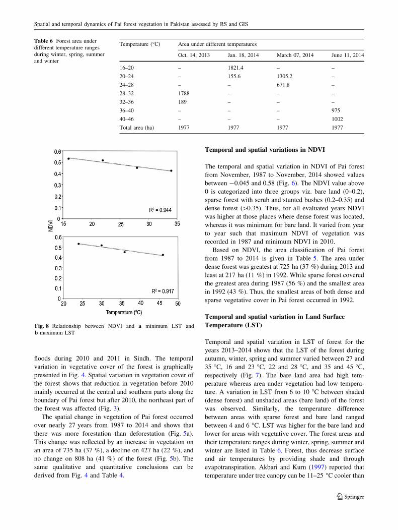
Fig. 8 Relationship between NDVI and a minimum LST and

b maximum LST

Spatial and temporal dynamics of Pai forest vegetation in Pakistan assessed by RS and GIS

123

on bare lands. A study conducted in Spain showed that

temperature differences between barren and forested lands

ranged up to 13 �C (Gomez et al. 2004). Regression

analysis of both minimum and maximum LST and NDVI

was carried out to assess the impact of extreme tempera-

tures on NDVI of the forest. An inverse relationship was

documented between LST and NDVI of Pai forest with

coefficients of determination of 0.944 and 0.917 when

NDVI was plotted against minimum and maximum LST,

respectively (Fig. 8). This might have been due to latent

heat transfer through evapotranspiration, lower heat

capacity, or thermal inertia of vegetation compared to soil

(Goward and Hope 1989). Similar results were reported by

Wilson et al. (2003), Small (2006), Yue and Tan (2007),

and Singh (2015).

Because increasing vegetative cover brings down the

LST, hence a healthy Pai forest will lower the surface and

air temperature, increase the humidity and thus decrease

the intensity of scorching heat in the area. Because

increasing vegetative cover reduces LST hence greater tree

density and canopy closure in Pai forest would be expected

to lower LST and thus air temperature as there is generally

a close correlation between LST and surface air tempera-

ture (Farina 2012).

Conclusion

Maximum reduction in the vegetation of Pai forest was

observed during 1992. Spatial change in vegetation of Pai

forest over about 27 years (1987–2014) revealed that there

was more increase in vegetation than reduction of vegeta-

tion. Thus, over 27 years, vegetation increased on 37.31 %

of the forest, decreased on 21.68 %, and there was no

change on 41.02 % of the forest. Variation of LST between

shaded (dense forest) and unshaded areas (bare land) of the

forest ranged from 6 to 10 �C. While the LST difference

between areas with sparse forest and bare land ranged

between 4 and 6 �C. Regression analysis of both minimum

and maximum LST and NDVI showed an inverse rela-

tionship between LST and NDVI of Pai forest with coef-

ficients of determination of 0.94 and 0.92, when NVI was

plotted against minimum and maximum LST, respectively.

Our results how that overall vegetation in forest

increased from 1552 ha (78.5 %) in 1987 to 1637 ha

(83 %) in 2014 though there was a significant decrease in

vegetation 1992. GIS and remote sensing tools can be used

for monitoring of spatial and temporal change in vegetation

as well as spatial change in LST of forests in arid regions.

These results can also be helpful for decision and policy

makers for developing an effective forest management

system and viable policies for the Pai and other arid forests.

References

Akbari H, Kurn D (1997) Peak power and cooling energy savings of

shade trees. Energy Build 25:139–148

Bhandari S, Phinn S, Gill T (2012) Preparing Landsat image time

series (LITS) for monitoring changes in vegetation phenology in

Queensland, Australia. Remote Sens 4:1856–1886

Braswell BH, Hagen SC, Frolking SE, Salas WA (2003) A

multivariable approach for mapping sub-pixel land cover

distributions using MISR and MODIS: application in the

Brazilian Amazon region. Remote Sens Environ

87(2–3):243–256

Dash P, Gottsche FM, Olesen FS, Fischer H (2002) Land surface

temperature and emissivity estimation from passive sensor data:

theory and practice-current trends. Int J Remote Sens

23(13):2563–2594

FAO (2001) State of World’s Forests 2001. Food and Agriculture

Organization of The United Nations, Rome

Farina A (2012) Exploring the relationship between land surface

temperature and vegetation abundance for urban heat island

mitigation in Seville, Spain. Thesis submitted to Department of

Earth and Ecosystem Sciences, Lund University

Faruqi S (2011) Into the Pai Forest. The Daily Dawn, December 16,

2011. (http://www.dawn.com/news/680945/into-the-pai-forest).

Accessed 5 Aug 2014

Gomez F, Jabaloyes J, Vano E (2004) Green zones in the future or

urban planning. J Urban Plan Dev 130(2):94–100

GoP (2003) Economic survey of Pakistan. Ministry of Finance,

Islamabad

Goward SN, Hope AS (1989) Evapotranspiration from combined

reflected solar and emitted terrestrial radiation: Preliminary FIFE

results from AVHRR data. Adv Space Res 9:239–249

Goward S, Irons J, Franks S, Arvidson T, Williams D, Faundeen J

(2006) Historical record of Landsat global coverage: mission

operations, NSLRSDA, and international cooperator stations.

Photogramm Eng Remote Sens 72:1155–1169

Hughes BJ, Martin GR, Reynolds SJ (2011) The use of Google Earth

(TM) satellite imagery to detect the nests of masked boobies

Sula dactylatra. Wildl Biol 17:210–216

Kawamura K, Akiyama T, Yokota H et al (2005) Quantifying grazing

intensities using geographic information systems and satellite

remote sensing in the Xilingol steppe region, Inner Mongolia,

China. Agric Ecosyst Environ 107(1):83–93

Kumar P, Meenu R, Pandey PC, Majumdar A, Nathawat MS (2010)

Monitoring of deforestation and forest degradation using remote

sensing and GIS: a case study of Ranchi in Jharkhand (India).

Report Opin 2(4):55–67

Li Z, Gu X, Dixon P, He Y (2008) Applicability of land surface

temperature (LST) estimates from AVHRR satellite image

composites in northern Canada. Prairie Perspect 11:119–130

Madin EMP, Madin JS, Booth DJ (2011) Landscape of fear visible

from space. Nat Sci Rep 1:14. doi:10.1038/srep00014

Masek JG, Vermote Huang C, Wolfe R, Cohen W, Hall F, Kutler J,

Nelson P (2008) North American forest disturbance mapped

from a decadal Landsat record. Remote Sens Environ

112:2914–2926

McInnes J, Vigiak O, Roberts AM (2011) Using Google Earth to map

gully extent in the West Gippsland region (Victoria, Australia).

19th International Congress on Modelling and Simulation, Perth,

Australia, 12–16 December. http://mssanz.org.au/modsim2011.

Accessed 5 Aug 2014

Mughal MS (2010) State of forests in Sindh as well as the economic

benefits flowing out of it. World Environment Day. Pakistan

Energy Congress. http://pecongress.org.pk/images/upload/books/

A. A. Siyal et al.

123

State%20of%20Forests%20in%20Sindh%20as%20well%20as%

20the%20Economic%20Benifits%20F.pdf

Nemani RR, Running SW (1997) Land cover characterization using

multitemporal red, near-IR, and thermal-IR data from NOAA/

AVHRR. Ecol Appl 7:79–90

Panhwar MH (2002) Water requirement of riverine area of Sindh.

Sindh Education Trust, Hyderabad, p 23

Pongratz J, Bounoua L, DeFries R, Morton D et al (2006) The impact

of land cover change on surface energy and water balance in

Mato Grosso, Brazil. Earth Interact 10:1–17

Potere D (2008) Horizontal positional accuracy of Google Earth’s

high resolution imagery archive. Sensors 8:7973–7981

Pringle H (2010) Google Earth shows clandestine worlds. Science

329:1008–1009. doi:10.1126/science.329.5995.1008

Qureshi R, Bhatti GR (2010) Floristic inventory of Pai forest, Nawab

Shah, Sindh, Pakistan. Pak J Bot 42(4):2215–2224

Rikimaru A (1999) Concept of FCD Mapping Model and Semi Expert

System. FCD Mapper’s User’s Guide. International Tropical

Timber Organization and Japan Overseas forestry Consultants

Association, p 90

Rouse JW, Haas RH, Schell JA, Deering DW (1974) Monitoring

vegetation systems in the Great Plains with ERTS. Proc. Third

ERTS-1 Symposium, NASA Goddard, NASA SP-351,

pp 309–317

Siddiqui ZM (2009) Sindh’s Pai forest faces land-grab. The Daily

Dawn, November 09, 2009. (http://www.dawn.com/news/

935660/sindh-s-pai-forest-faces-land-grab). Accessed 15 Aug

2014

Singh RB (2015) Urban development challenges, risks and resilience

in Asian mega cities. Advances in geographical and environ-

mental sciences. Springer, Tokyo, p 92

Small C (2006) Comparative analysis of urban reflectance and surface

temperature. Remote Sens Environ 104:168–189

Sunderland TCH, Powell B, Ickowitz A et al (2013) Food security and

nutrition: the role of forests. Center for International Forestry

Research (CIFOR), Bogor

Telesca L, Lasaponara R, Lanorte A (2006) 1/fa Fluctuations in the

time dynamics of Mediterranean forest ecosystems by using

normalized difference vegetation index satellite data. Phys A

361(2):699–706

UNEP (2011) Forests in a green economy: a synthesis. United

Nations Environment Programme, St-Martin-Bellevue

van Leeuwen TT, Frank AJ, Jin Y, Smyth P et al (2011) Optimal use

of land surface temperature data to detect changes in tropical

forest cover. J Geophys Res 116:1–16

Wickham JD, Wade TG, Kurt HR (2012) Comparison of cropland and

forest surface temperatures across the conterminous United

States. Agric For Meteorol 166–167:137–143

Wilson JS, Clay M, Martin E et al (2003) Evaluating environmental

influences of zoning in urban ecosystems with remote sensing.

Remote Sens Environ 86(2003):303–321

Wulder MA, White JC, Goward SN, Masek JG, Irons JR, Herold M,

Cohen WB, Loveland TR, Woodcock CE (2008) Landsat

continuity: issues and opportunities for land cover monitoring.

Remote Sens Environ 112:955–969

WWF (2008) Detailed Ecological Assessment Report 2008—Pai

Forest and Keti Shah. Indus for all program

Xiao XM, Zhang Q, Braswell B et al (2004) Modeling gross primary

production of temperate deciduous broadleaf forest using

satellite images and climate data. Remote Sens Environ

91:256–270

Xie Y, Sha Z, Yu M (2008) Remote sensing imagery in vegetation

mapping: a review. J Plant Ecol 1(1):9–23

Yang J, Wang Y, David R (2007) Estimating air temperature profiles

in forest canopy using empirical models and Landsat data. For

Sci 53(1):93–99

Yue W, Tan W (2007) The relationship between land surface

temperature and NDVI with remote sensing: application to

Shanghai Landsat 7 ETM? data. Int J Remote Sens

28(5):3205–3226

Spatial and temporal dynamics of Pai forest vegetation in Pakistan assessed by RS and GIS

123