International Symposium on Outfall Systems, May 15-18, 2011, Mar del Plata, Argentina

Spatial Analysis and Dilution Estimation of Foz do Arelho

Outfall Using Observations Gathered by an AUV P. Ramos* and N. Abreu** * INESC Porto, Campus da FEUP, Rua Dr. Roberto Frias 378, 4200-465 Porto, Portugal ISCAP – IPP, Rua Jaime Lopes Amorim s/n, 4465-004 S. Mamede de Infesta, Portugal (E-mail: pramos@inescporto.pt)

** INESC Porto, Campus da FEUP, Rua Dr. Roberto Frias, 378, 4200-465 Porto, Portugal (E-mail: nabreu@inescporto.pt) Abstract

Autonomous Underwater Vehicles have already been shown to be very useful for monitoring routine of ocean outfalls. The major advantage of this technology over traditional methods is the ability to collect high-resolution data which can be very valuable for environmental impact assessment and comparison with plume prediction models. Once the data has been collected in the field it is necessary to extrapolate from monitoring samples to unsampled locations. Geostatistics has been used with success to obtain spatial information of natural resources. In this work geostatistics is used to model and map the spatial distribution of temperature and salinity measurements gathered by MARES AUV in a monitoring campaign to Foz do Arelho outfall. The kriged maps show the spatial variation of these parameters in the area studied and from them it is possible to identify the effluent plume from the receiving waters in the vicinity of the discharge. The salinity distribution is then used to estimate dilution. The results demonstrate that this methodology provides good estimates of the dispersion of effluent which are valuable for assessing the environmental impact and managing sea outfalls. Keywords Spatial analysis; plume dilution estimation; monitoring; autonomous underwater vehicles

INTRODUCTION

Autonomous Underwater Vehicles (AUVs) already demonstrated to be very appropriate for high-resolution surveys of small features such as outfall plumes. Some of the advantages of these platforms include: easier field logistics, low cost per deployment, good spatial coverage, sampling over repeated sections and capability of feature-based or adaptive sampling. Demands for more reliable model predictions, and predictions of quantities that have received little attention in the past are now increasing. These are driven by increasing environmental awareness, more stringent environmental standards, and application of diffusion theory in new areas. Although very chaotic due to turbulent diffusion, the effluent’s dispersion process tends to a natural variability mode when the plume stops rising and the intensity of turbulent fluctuations approaches to zero ([1]). It is likely that after this point the pollutant substances are spatially correlated. In this case, geostatistics appears to be an appropriate technique to model the spatial distribution of the effluent. In fact, geostatistics has been used with success to analyze and characterize the spatial variability of soil properties, to obtain information for assessing water and wind resources, to design sampling strategies for monitoring estuarine sediments, to study the thickness of effluent-affected sediment in the vicinity of wastewater discharges, to obtain information about the spatial distribution of sewage pollution in coastal sediments, among others. As well as giving the estimated values, geostatistics provides a measure of the accuracy of the estimate in the form of the kriging variance. This is one of the advantages of geostatistics over traditional methods of assessing pollution. In this study we use ordinary block kriging to model and map the spatial distribution of temperature and salinity measurements gathered with MARES AUV in a monitoring campaign to Foz do Arelho outfall, aiming to distinguish the effluent plume from the receiving waters, characterize its spatial variability in the vicinity of the discharge and estimate dilution. In this work geostatistics is used to model and map the spatial distribution of temperature and salinity measurements gathered by MARES AUV in a monitoring campaign to Foz do Arelho outfall, with the aim of distinguishing

the effluent plume from the receiving waters, characterizing its spatial variability in the vicinity of the discharge and estimating dilution. In the next section MARES AUV's physical and operating characteristics are fully described. In the third section the methodology of the spatial analysis is applied to the case study. In the forth section the spatial distribution of salinity is used to estimate dilution. Finally we discuss the results and give the conclusions. MARES AUV

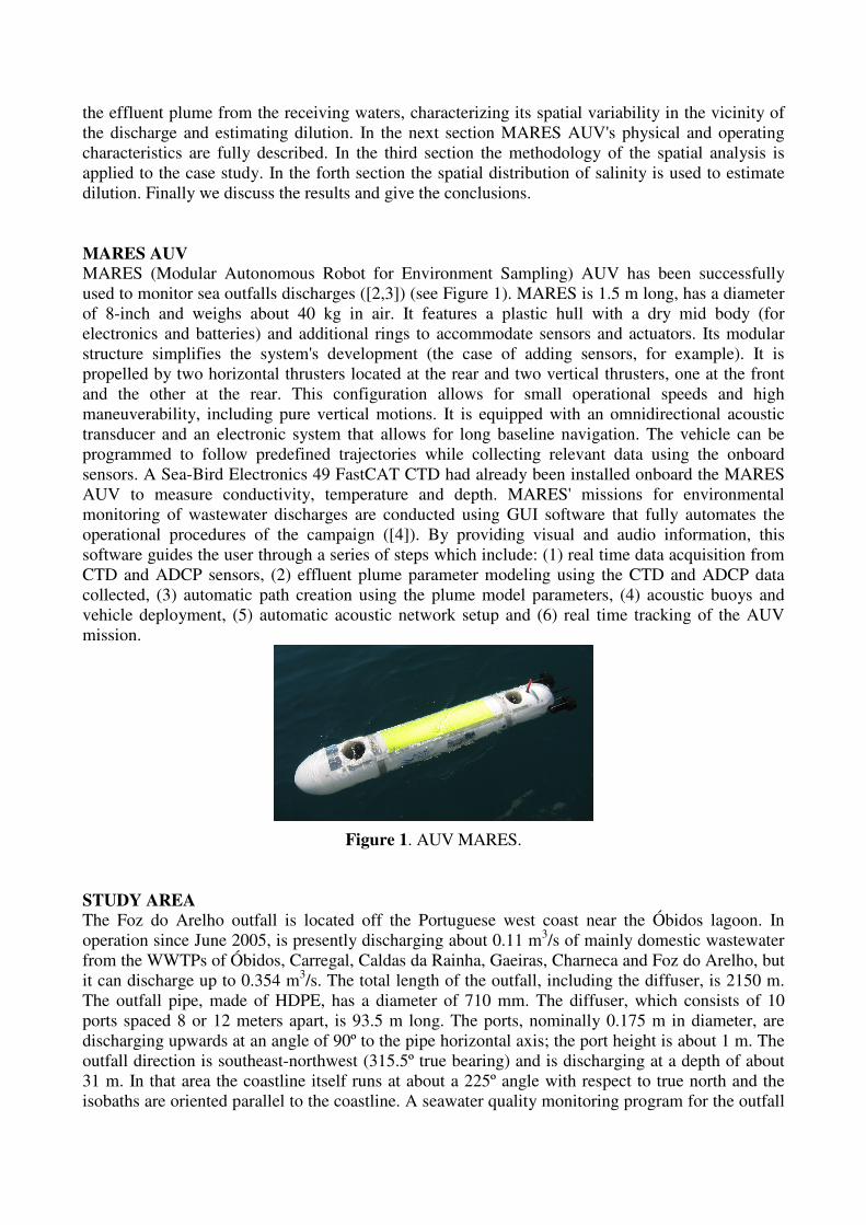
MARES (Modular Autonomous Robot for Environment Sampling) AUV has been successfully used to monitor sea outfalls discharges ([2,3]) (see Figure 1). MARES is 1.5 m long, has a diameter of 8-inch and weighs about 40 kg in air. It features a plastic hull with a dry mid body (for electronics and batteries) and additional rings to accommodate sensors and actuators. Its modular structure simplifies the system's development (the case of adding sensors, for example). It is propelled by two horizontal thrusters located at the rear and two vertical thrusters, one at the front and the other at the rear. This configuration allows for small operational speeds and high maneuverability, including pure vertical motions. It is equipped with an omnidirectional acoustic transducer and an electronic system that allows for long baseline navigation. The vehicle can be programmed to follow predefined trajectories while collecting relevant data using the onboard sensors. A Sea-Bird Electronics 49 FastCAT CTD had already been installed onboard the MARES AUV to measure conductivity, temperature and depth. MARES' missions for environmental monitoring of wastewater discharges are conducted using GUI software that fully automates the operational procedures of the campaign ([4]). By providing visual and audio information, this software guides the user through a series of steps which include: (1) real time data acquisition from CTD and ADCP sensors, (2) effluent plume parameter modeling using the CTD and ADCP data collected, (3) automatic path creation using the plume model parameters, (4) acoustic buoys and vehicle deployment, (5) automatic acoustic network setup and (6) real time tracking of the AUV mission.

Figure 1. AUV MARES. STUDY AREA

The Foz do Arelho outfall is located off the Portuguese west coast near the Óbidos lagoon. In operation since June 2005, is presently discharging about 0.11 m3/s of mainly domestic wastewater from the WWTPs of Óbidos, Carregal, Caldas da Rainha, Gaeiras, Charneca and Foz do Arelho, but it can discharge up to 0.354 m3/s. The total length of the outfall, including the diffuser, is 2150 m. The outfall pipe, made of HDPE, has a diameter of 710 mm. The diffuser, which consists of 10 ports spaced 8 or 12 meters apart, is 93.5 m long. The ports, nominally 0.175 m in diameter, are discharging upwards at an angle of 90º to the pipe horizontal axis; the port height is about 1 m. The outfall direction is southeast-northwest (315.5º true bearing) and is discharging at a depth of about 31 m. In that area the coastline itself runs at about a 225º angle with respect to true north and the isobaths are oriented parallel to the coastline. A seawater quality monitoring program for the outfall

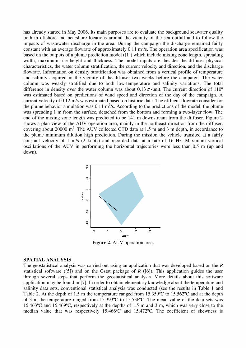
has already started in May 2006. Its main purposes are to evaluate the background seawater quality both in offshore and nearshore locations around the vicinity of the sea outfall and to follow the impacts of wastewater discharge in the area. During the campaign the discharge remained fairly constant with an average flowrate of approximately 0.11 m3/s. The operation area specification was based on the outputs of a plume prediction model ([1]) which include mixing zone length, spreading width, maximum rise height and thickness. The model inputs are, besides the diffuser physical characteristics, the water column stratification, the current velocity and direction, and the discharge flowrate. Information on density stratification was obtained from a vertical profile of temperature and salinity acquired in the vicinity of the diffuser two weeks before the campaign. The water column was weakly stratified due to both low-temperature and salinity variations. The total difference in density over the water column was about 0.13σ -unit. The current direction of 110º was estimated based on predictions of wind speed and direction of the day of the campaign. A current velocity of 0.12 m/s was estimated based on historic data. The effluent flowrate consider for the plume behavior simulation was 0.11 m3/s. According to the predictions of the model, the plume was spreading 1 m from the surface, detached from the bottom and forming a two-layer flow. The end of the mixing zone length was predicted to be 141 m downstream from the diffuser. Figure 2 shows a plan view of the AUV operation area, mainly in the northeast direction from the diffuser, covering about 20000 m2. The AUV collected CTD data at 1.5 m and 3 m depth, in accordance to the plume minimum dilution high prediction. During the mission the vehicle transited at a fairly constant velocity of 1 m/s (2 knots) and recorded data at a rate of 16 Hz. Maximum vertical oscillations of the AUV in performing the horizontal trajectories were less than 0.5 m (up and down).

Figure 2. AUV operation area.

SPATIAL ANALYSIS

The geostatistical analysis was carried out using an application that was developed based on the R statistical software ([5]) and on the Gstat package of R ([6]). This application guides the user through several steps that perform the geostatistical analysis. More details about this software application may be found in [7]. In order to obtain elementary knowledge about the temperature and salinity data sets, conventional statistical analysis was conducted (see the results in Table 1 and Table 2. At the depth of 1.5 m the temperature ranged from 15.359ºC to 15.562ºC and at the depth of 3 m the temperature ranged from 15.393ºC to 15.536ºC. The mean value of the data sets was 15.463ºC and 15.469ºC, respectively at the depths of 1.5 m and 3 m, which was very close to the median value that was respectively 15.466ºC and 15.472ºC. The coefficient of skewness is

relatively low (-0.309) for the 1.5 m data set and not very high (-0.696) for the 3 m data set, indicating that in the first case the histogram is approximately symmetric and in the second case that distribution is only slightly asymmetric. The very low values of the coefficient of variation (0.002 and 0.001) reflect the fact that the histograms do not have a tail of high values. At the depth of 1.5 m the salinity ranged from 35.957 psu to 36.003 psu and at the depth of 3 m the salinity ranged from 35.973 psu to 36.008 psu. The mean value of the data sets was 35.991 psu and 35.996 psu, respectively at the depths of 1.5 m and 3 m, which was very close to the median value that was respectively 35.990 and 35.998 psu. The coefficient of skewness is not to much high in both data sets (-0.63 and -1.1) indicating that distributions are only slightly asymmetric. The very low values of the coefficient of variation (0.0002 and 0.0001) reflect the fact that the histograms do not have a tail of high values. The ordinary kriging method works better if the distribution of the data values is close to a normal distribution. Therefore, it is interesting to see how close the distribution of the data values comes to being normal. Figure 3 shows the plots of the normal distribution adjusted to the histograms of the temperature measured at depths of 1.5 m and 3 m, and Figure 4 shows the plots of the normal distribution adjusted to the histograms of the salinity measured at depths of 1.5 m and 3 m. Apart from some erratic high values it can be seen that the histograms are reasonably close to the normal distribution. For the purpose of this analysis, the temperature and the salinity measurements were divided into a modeling set (comprising 90% of the samples) and a validation set (comprising 10% of the samples). Modeling and validation sets were then compared, using Student's-t test, to check that they provided unbiased sub-sets of the original data. Furthermore, sample variograms for the modeling sets were constructed using the Matheron's method-of-moments estimator (MME) estimator [8] and the Cressie estimator (CRE) [9]. This robust estimator was chosen to deal with outliers and enhance the variogram's spatial continuity. An estimation of semivariance was carried out using a lag distance of 2 m [10,11].

Table 1. Summary statistics of temperature measurements.

Temperature@1.5 m Temperature@3 m

Samples 20,026 10,506

Mean 15.463ºC 15.469ºC

Median 15.466ºC 15.472ºC

Minimum 15.359ºC 15.393ºC

Maximum 15.562ºC 15.536ºC

Coefficient of skewness -0.31 -0.70

Coefficient of variation 0.002 0.001

Table 2. Summary statistics of salinity measurements.

Salinity@1.5 m Salinity@3 m

Samples 20,026 10,506

Mean 35.991 psu 35.996 psu

Median 35.990 psu 35.998 psu

Minimum 35.957 psu 35.973 psu

Maximum 36.003 psu 36.008 psu

Coefficient of skewness -0.63 -1.1

Coefficient of variation 0.0002 0.0001

Figure 3. Histograms of temperature measurements at depths of 1.5 m (left) and 3 m (right).

Figure 4. Histograms of salinity measurements at depths of 1.5 m (left) and 3 m (right).

Table 3. Parameters of the fitted variogram models for temperature measured at depths of 1.5 and 3.0 m.

Depth Variogram Estimator

Model Nugget Sill Range

1.5 MME Matern ( 0.4)ν = 0.000 0.001 75.0

CRE Matern ( 0.5)ν = 0.000 0.002 80.1

3.0 MME Matern ( 0.3)ν = 0.000 0.0002 101.3

CRE Matern ( 0.7)ν = 0.000 0.002 107.5

Table 4. Parameters of the fitted variogram models for salinity measured at depths of 1.5 and 3.0 m.

Depth Variogram Estimator

Model Nugget Sill Range

1.5 MME Matern ( 0.6)ν = 0.436 11.945 134.6

CRE Matern ( 0.6)ν = 0.153 10786.109

51677.1

3.0 MME Matern ( 0.8)ν = 0.338 11.724 181.6

CRE Gaussian 0.096 120.578 390.1

Table 3 and Table 4 show the parameters of the fitted models to the omnidirectional sample variograms constructed using MME and CRE estimators. All the variograms were fitted to Matern models (for several shape parameters ν ) with the exception to the salinity data measured at the depth of 3 m. The range value (in meters) is an indicator of extension where autocorrelation exists. The variograms of salinity show significant differences in range. The autocorrelation distances are always larger for the CRE estimator which may demonstrate the enhancement of the variogram's spatial continuity. All variograms have low nugget values which indicates that local variations could be captured due to the high sampling rate and to the fact that the variables under study have strong spatial dependence. Anisotropy was investigated by calculating directional variograms. However, no anisotropy effect could be shown. The block kriging method was preferred since it produced smaller prediction errors and smoother maps than the point kriging [12]. Using the 90% modeling sets of the two depths, a two-dimensional ordinary block kriging, with blocks of 10 10× m2, was applied to estimate temperature at the locations of the 10% validation sets. The validation results for both parameters measured at depths of 1.5 m and 3 m depths are shown in Table 5 and Table 6. At both depths temperature was best estimated by the variogram constructed using CRE. Salinity at the depth of 1.5 m was best estimated by the variogram constructed using CRE and at the depth of 3 m was best estimated using the Gaussian model with the MME. The difference in performance between the two estimators: block kriging using the MME estimator (MBK) or block kriging using the CRE estimator (CBK) is not substantial. Figure 5 shows the omnidirectional sample variograms for temperature at the depth of 1.5 m and 3 m fitted by the preferred models. Figure 6 shows the omnidirectional sample variograms for salinity at the depth of 1.5 m and 3 m fitted by the preferred models. The R2 value for the temperature at the depth of 1.5 m was 0.9211 and the RMSE was 0.0088248ºC, and at the depth of 3 m was 0.8827 and the RMSE was 0.0058316ºC (Table 5). The R2 value for the salinity at the depth of 1.5 m was 0.9513 and the RMSE was 0.0016435 psu, and at the depth of 3 m was 0.8982 and the RMSE was 0.0019793 psu (Table 6).

Table 5. Cross-validation results for the temperature maps at depths of 1.5 and 3 m.

Depth Method R2 ME MSE RMSE

1.5 MBK 0.9184 2.0174e-4 8.0530e-5 9739e-3

CBKa 0.9211 1.6758e-4 7.7880e-5 8248e-3

3.0 MBK 0.8748 1.0338e-4 3.6295e-5 6.0244e-3

CBKa 0.8827 0.6538e-4 3.4008e-5 5.8316e-3 a The preferred model.

Table 6. Cross-validation results for the salinity maps at depths of 1.5 and 3 m.

Depth Method R2 ME MSE RMSE

1.5 MBK 0.9471 3.1113e-5 2.8721e-6 1.6947e-3

CBKa 0.9513 -3.1579e-5 2.7010e-6 1.6435e-3

3.0 MBK 0.8982 -7.1735e-5 3.9175e-6 1.9793e-3

CBKa 0.7853 -8.1264e-5 8.2589e-6 2.8738e-3 a The preferred model.

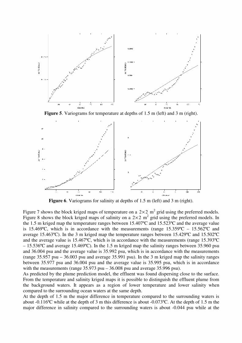
Figure 5. Variograms for temperature at depths of 1.5 m (left) and 3 m (right).

Figure 6. Variograms for salinity at depths of 1.5 m (left) and 3 m (right).

Figure 7 shows the block kriged maps of temperature on a 2 2× m2 grid using the preferred models. Figure 8 shows the block kriged maps of salinity on a 2 2× m2 grid using the preferred models. In the 1.5 m kriged map the temperature ranges between 15.407ºC and 15.523ºC and the average value is 15.469ºC, which is in accordance with the measurements (range 15.359ºC – 15.562ºC and average 15.463ºC). In the 3 m kriged map the temperature ranges between 15.429ºC and 15.502ºC and the average value is 15.467ºC, which is in accordance with the measurements (range 15.393ºC – 15.536ºC and average 15.469ºC). In the 1.5 m kriged map the salinity ranges between 35.960 psu and 36.004 psu and the average value is 35.992 psu, which is in accordance with the measurements (range 35.957 psu – 36.003 psu and average 35.991 psu). In the 3 m kriged map the salinity ranges between 35.977 psu and 36.004 psu and the average value is 35.995 psu, which is in accordance with the measurements (range 35.973 psu – 36.008 psu and average 35.996 psu). As predicted by the plume prediction model, the effluent was found dispersing close to the surface. From the temperature and salinity kriged maps it is possible to distinguish the effluent plume from the background waters. It appears as a region of lower temperature and lower salinity when compared to the surrounding ocean waters at the same depth. At the depth of 1.5 m the major difference in temperature compared to the surrounding waters is about -0.116ºC while at the depth of 3 m this difference is about -0.073ºC. At the depth of 1.5 m the major difference in salinity compared to the surrounding waters is about -0.044 psu while at the

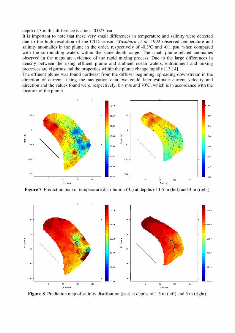
depth of 3 m this difference is about -0.027 psu. It is important to note that these very small differences in temperature and salinity were detected due to the high resolution of the CTD sensor. Washburn et al. 1992 observed temperature and salinity anomalies in the plume in the order, respectively of -0.3ºC and -0.1 psu, when compared with the surrounding waters within the same depth range. The small plume-related anomalies observed in the maps are evidence of the rapid mixing process. Due to the large differences in density between the rising effluent plume and ambient ocean waters, entrainment and mixing processes are vigorous and the properties within the plume change rapidly [13,14]. The effluent plume was found northeast from the diffuser beginning, spreading downstream in the direction of current. Using the navigation data, we could later estimate current velocity and direction and the values found were, respectively, 0.4 m/s and 70ºC, which is in accordance with the location of the plume.

Figure 7. Prediction map of temperature distribution (ºC) at depths of 1.5 m (left) and 3 m (right).

Figure 8. Prediction map of salinity distribution (psu) at depths of 1.5 m (left) and 3 m (right).

Figure 9 shows the variance of the estimation error (kriging variance) for the maps of temperature distribution at depths of 1.5 m and 3 m. The standard deviation of the estimation error is less than 0.0195ºC at the depth of 1.5 m and less than 0.0111ºC at the depth of 3 m. It’s interesting to observe that, as expected, the variance of the estimation error is less the closer is the prediction from the trajectory of the vehicle. The dark blue regions correspond to the trajectory of MARES AUV.

Figure 9. Variance of the estimation error for the maps of temperature distribution at depths of

1.5 m (left) and 3 m (right). DILUTION ESTIMATION

Environmental effects are all related to concentration C of a particular contaminant X . Defining

aC as the background concentration of substance X in ambient water and 0C as the concentration

of X in the effluent discharge, the local dilution comes as follows [15]:

0 ,a

a

C CS

C C

−=

− (1)

which can be rearranged to give 0

1 1a

SC C C

S S

− = +

. In the case of variability of the

background concentration of substance X in ambient water the local dilution is given by

0 0a

a

C CS

C C

−=

− (2)

where 0aC is the background concentration of substance X in ambient water at the discharge depth.

This expression in (2) can be arranged to give ( )0 0

1a aC C C C

S

= + −

, which in simple terms

means that the increment of concentration above background is reduced by the dilution factor S from the point of discharge to the point of measurement of C . Using salinity distribution at depths of 1.5 m and 3 m we estimated dilution using Equation 2 (see the contour maps in Figure 10). We assumed 0 2.3C = psu, 0 35.93

aC = psu, 36.008

aC = psu at 1.5 m depth and 36.006

aC = psu at 3 m

depth. The minimum dilution observed at the depth of 1.5 m was 705 and at the depth of 3.0 m was 1164 which is in accordance with Portuguese legislation that suggests that outfalls should be designed to assure a minimum dilution of 50 at the surface [16].

Figure 10. Dilution maps at depths of 1.5 m (left) and 3 m (right).

CONCLUSION

Through geostatistical analysis of temperature and salinity obtained by an AUV at depths of 1.5 m and 3 m in an ocean outfall monitoring campaign it was possible to produce kriged maps of the sewage dispersion in the field. The spatial variability of the sampled data has been analyzed and the results indicated an approximated normal distribution of the temperature and salinity measurements, which is desirable. The Matheron's classical estimator and Cressie and Hawkins' robust estimator were then used to compute the omnidirectional variograms that were fitted to Matern models (for several shape parameters) and to a Gaussian model. The performance of each competing model was compared using a split-sample approach. In the case of temperature, the validation results, using a two-dimensional ordinary block kriging, suggested the Matern model ( 0.5ν = – 1.5m and 0.7ν = – 3 m) with semivariance estimated by CRE. In the case of salinity, the validation results, using a two-dimensional ordinary block kriging, suggested the Matern model ( 0.6ν = – 1.5 m and 0.8ν = – 3 m) with semivariance estimated by CRE, for the depth of 1.5 m, and with semivariance estimated by MME, for the depth of 3 m. The difference in performance between the two estimators was not substantial. Block kriged maps of temperature and salinity at depths of 1.5 m and 3 m show the spatial variation of these parameters in the area studied and from them it is possible to identify the effluent plume that appears as a region of lower temperature and lower salinity when compared to the surrounding waters, northeast from the diffuser beginning, spreading downstream in the direction of current. Using salinity distribution at depths of 1.5 m and 3 m we estimated dilution at those depths. The values found are in accordance with Portuguese legislation. The results presented in this paper demonstrate that geostatistical methodology can provide good estimates of the dispersion of effluent that are very valuable in assessing the environmental impact and managing sea outfalls. ACKNOWLEDGEMENT

This work was partially funded by the Foundation for Science and Technology (FCT) under the Program for Research Projects in all scientific areas (Programa de Projectos de Investigação em todos os domínos científicos) in the context of WWECO project - Environmental Assessment and Modeling of Wastewater Discharges using Autonomous Underwater Vehicles Bio-optical Observations (Ref. PTDC/MAR/74059/2006).

REFERENCES

[1] C. D. Hunt, A. D. Mansfield, M. J. Mickelson, C. S. Albro, W. R. Geyer, and P. J. W. Roberts, “Plume tracking and dilution of effluent from the Boston sewage outfall”, Marine Environmental

Research, vol. 70, pp. 150–161, 2010. [2] P. Ramos and N. Abreu, “Using an AUV for Assessing Wastewater Discharges Impact: An Approach Based on Geostatistics”, Marine Technology Society Journal, vol. 45, no. 2, 2011. [3] P. Ramos, M. V. Neves, and F. L. Pereira, “Mapping and Initial Dilution Estimation of a Sewage Outfall Plume using an Autonomous Underwater Vehicle”, Continental Shelf Research, no. 27, pp. 583–593, 2007. [4] N. Abreu, A. Matos, P. Ramos, and N. Cruz, “Automatic interface for AUV mission planning and supervision”, in MTS/IEEE International Conference Oceans 2010, Seattle, USA, September 20-23 2010. [5] R Development Core Team, “The R Project for Statistical Computing”, 2011. [Online]. Available: http://www.r-project.org/ [6] R. S. Bivand, E. J. Pebesma, and V. Gómez-Rubio, Applied spatial data analysis with R, UseR! Series, Springer, 2008, ISBN: 97 -0-387-78170-9. [7] N. Abreu and P. Ramos, “An integrated application for geostatistical analysis of sea outfall discharges based on R software”, in MTS/IEEE International Conference Oceans 2010, Seattle, USA, September 20-23 2010. [8] G. Matheron, Les variables régionalisées et leur estimation: une application de la théorie des

fonctions aléatoires aux sciences de la nature, F. Masson, Ed., Paris, 1965. [9] N. Cressie and D. M. Hawkins, “Robust estimation of the variogram, I,” Jour. Int. Assoc. Math.

Geol., vol. 12, no. 2, pp. 115–125, 1980. [10] E. H. Isaaks and R. M. Srivastava, Applied geostatistics, O. U. Press, Ed., New York Oxford, 1989, ISBN 0-19-505012-6-ISBN 0-19-505013- 4 (pbk.). [11] N. Cressie, Statistics for spatial data, A. W. I. Publication, Ed., New York, 1993. [12] P. Goovaerts, Geostatistics for natural resources evaluation, Applied Geostatistics Series, O. U. Press, Ed., 1997, ISBN13: 9780195115383, ISBN10: 0195115384. [13] L. Washburn, B. H. Jones, A. Bratkovich, T. D. Dickey, and M.-S. Chen, “Mixing, Dispersion, and Resuspension in Vicinity of Ocean Wastewater Plume”, Journal of Hydraulic Engineering, ASCE, vol. 118, no. 1, pp. 38–58, Jan. 1992. [14] Petrenko, A.A., Jones, B.H., Dickey, T.D.: “Shape and initial dilution of Sand Island, Hawaii sewage plume”, Journal of Hydraulic Engineering, ASCE Vol. 124, No. 6, pp. 565-571, 1998. [15] H. B. Fischer, J. E. List, R. C. Y. Koh, J. Imberger, and N. H. Brooks, Mixing in Inland and

Coastal Waters, Academic Press, 1979. [16] INAG, Linhas de Orientação Metodológica para a Elaboração de Estudos Técnicos Necessários para Cumprir o Artigo 7º do D.L. 152/97. Descargas em Zonas Menos Sensíveis, Instituto da Água, Ministério do Ambiente. Lisboa, 1998.