SPASELOC: AN ADAPTIVE SUBPROBLEM ALGORITHM FOR …

SIAM J. OPTIM. c© 2006 Society for Industrial and Applied MathematicsVol. 17, No. 4, pp. 1102–1128

SPASELOC: AN ADAPTIVE SUBPROBLEM ALGORITHM FORSCALABLE WIRELESS SENSOR NETWORK LOCALIZATION∗

MICHAEL W. CARTER† , HOLLY H. JIN‡ , MICHAEL A. SAUNDERS§ , AND YINYU YE§

Abstract. An adaptive rule-based algorithm, SpaseLoc, is described to solve localization prob-lems for ad hoc wireless sensor networks. A large problem is solved as a sequence of very smallsubproblems, each of which is solved by semidefinite programming relaxation of a geometric opti-mization model. The subproblems are generated according to a set of sensor/anchor selection rules.Computational results compared with existing approaches show that the SpaseLoc algorithm scaleswell and provides excellent localization accuracy.

Key words. sensor localization, semidefinite programming, large-scale optimization

AMS subject classifications. 49M37, 65K05, 90C30

DOI. 10.1137/040621600

1. Introduction. Ad hoc wireless sensor networks may contain hundreds oreven tens of thousands of inexpensive devices (sensors) that can communicate withtheir neighbors within a limited radio range. By relaying information to each other,they can transmit signals to a command post anywhere within the network. Theyhave many practical uses in areas such as military applications [15], environment orindustrial control and monitoring [7, 9], wildlife monitoring [24], and security moni-toring [15]. For example, Southern California Edison’s Nuclear Generating Station inSan Onofre, CA, has deployed wireless mesh networked sensors from Dust Networks,Inc. to obtain real-time trend data [9]. These data are used to predict which motorsare about to fail, so they could be preemptively rebuilt or replaced during scheduledmaintenance periods. The use of a wireless sensor network saves the station moneyand avoids potential machine shutdown. Implementation of a sensor localization al-gorithm would provide a service that eliminates the need to record every sensor’slocation and its associated ID number in the network.

Wireless sensor networks are potentially important enablers for many other ad-vanced applications. A huge variety of applications lie ahead. By 2008, there couldbe 100 million wireless sensors in use, up from about 200,000 in 2005, according tothe market-research company Harbor Research. The worldwide market for wirelesssensors, it says, will grow from $100 million in 2005 to more than $1 billion by 2009[18]. This is motivating great effort in academia and industry to explore effective waysto build sensor networks with feature-rich services [12].

One of the important inputs these services build upon is the exact locations ofall sensors in the network. The need for sensor localization arises because accurate

∗Received by the editors December 27, 2004; accepted for publication (in revised form) February27, 2006; published electronically December 5, 2006.

http://www.siam.org/journals/siopt/17-4/62160.html†Department of Mechanical and Industrial Engineering, University of Toronto, Toronto, ON,

Canada M5S 3G8 ([email protected]).‡Department of Management Science and Engineering, Stanford University, Stanford, CA 94305-

4026, and Department of Mechanical and Industrial Engineering, University of Toronto, Toronto,ON, Canada M5S 3G8 ([email protected]). The author was partially supported by RobertBosch Corporation.

§Department of Management Science and Engineering, Stanford University, Stanford, CA 94305-4026 ([email protected], [email protected]).

1102

SPASELOC: A SCALABLE SENSOR LOCALIZATION ALGORITHM 1103

1 ≤ i < j ≤ s|s+1 ≤ k ≤ n

︸︷︷︸|︸︷︷︸

s sensors m anchors

Fig. 1.1. Indexing of sensors and anchors.

locations are known for only some of the sensors (which are called anchors). If thenetworks are to achieve their purpose, the locations of the remaining sensors mustbe determined. One approach to localizing these sensors with unknown locations isto use known anchor locations and distance measurements that neighboring sensorsand anchors obtain among themselves. The mathematical problem is to estimate allsensors’ locations using a sparse data matrix of noisy distance measurements. Thisleads to a large, nonconvex, constrained optimization problem. Large networks maycontain many thousands of sensors, whose locations should be determined accuratelyand quickly.

1.1. Problem definition. Sensor localization for ad hoc wireless sensor net-works aims to find the locations of all sensors in the network, given pairwise distancemeasurements among some of the sensors and known locations of some of the sensors.The sensors with known locations are called anchors. From now on, sensor generallymeans unlocalized sensor, excluding anchors. A node is any sensor or anchor.

We use a constrained optimization approach to estimate the sensors’ locations.The following input, output, and objectives are considered.

InputTotal points: n, the total number of nodes in the network.Unknown points : s sensors, whose locations xi ∈ R2, i = 1, . . . , s, are to be de-

termined. (We assume the points are on a plane here, but the approach isextended to three dimensions in Jin’s thesis [14].)

Known points: m anchors, whose locations ak ∈ R2, k = s + 1, . . . , n, are known.(Note that we put anchors at the end of the total points’ list without lossof generality, and that n = s + m. Index k is specific for indexing anchors.Refer to Figure 1.1 for node indexing.)

Known distance measurements: The nonzero elements of a sparse matrix d con-taining the readings of certain ranging devices for estimating the distancebetween two points. dij is the distance measurement between two sensors xi

and xj (i < j ≤ s), and dik is the distance measurement between some sensorxi and anchor ak (i ≤ s < k). The distance measurements are constant dataand generally have errors.

OutputLocations: Estimated locations xi for s sensors.

ObjectivesAccuracy : Minimal errors in the estimated sensor locations.Speed : Fast enough for real-time applications (e.g., networks with moving sensors).Scalability : Suitable for large-scale deployment (with tens of thousands of nodes).

1.2. Notation. The Euclidean distance between two vectors v and w is definedto be ‖v −w‖, where ‖ · ‖ always means the 2-norm. Nodes are said to be connected

if the associated measurements dij or dik exist. The remaining elements of d are zero.

1104 M. W. CARTER, H. H. JIN, M. A. SAUNDERS, AND Y. YE

If a measurement does exist between node i and j but it is zero (i and j are at the

same spot), we do not set dij to zero: we set it to machine precision ε instead to

distinguish from the case of dij = 0 when two nodes’ distance is beyond the sensordevice’s measuring range.

1.3. Related research work. Sensor localization in ad hoc wireless networkshas been a booming research area recently. Hightower and Boriello [12] give an ex-tensive review of the area and available methods. There are many ways to solve thelocalization problem [6, 8, 10, 13, 17, 19, 20, 21, 22], with two main ones based ontriangulation and optimization.

Triangulation methods estimate node locations based on distance measurementsbetween neighboring nodes, and some algorithms use iterative steps to localize allsensors.

Early work using optimization techniques is reported by Doherty, El Ghaoui, andPister [8]. Ideally the Euclidean distance between neighboring nodes should be fittedin some near-equality sense to the distance measurements:

‖xi − xj‖ ≈ dij and ‖xi − ak‖ ≈ dik.(1.1)

Doherty, El Ghaoui, and Pister formulate a convex optimization model by treatingthe constraints as ‖xi−xj‖ ≤ dij and ‖xi−ak‖ ≤ dik, and by including certain otherconvex constraints. This formulation takes advantage of available optimization algo-rithms, including those for convex optimization. However, the method needs sufficientanchors to be on the boundary of the localization area for it to work effectively.

Biswas and Ye [2] work with the near-equality constraints (1.1), and more im-portantly introduced a semidefinite programming (SDP) relaxation method in orderto retain the benefits of convex optimization. They report that their method yieldsmore accuracy than the approach in [8].

The SDP relaxation approach can solve small problems effectively. The paper[2] reports a few seconds of laptop execution time for a 50-node localization problem.However, the number of constraints in the SDP model is O(n2), where n is the numberof nodes in the network. Even a few-hundred-node problem leads to excessive memoryand computation time by available SDP solvers such as DSDP (Benson, Ye, andZhang [1]) and SeDuMi (Sturm [23]). These solvers are effective for SDP problemswith dimension and number of constraints up to a few thousand.

Tseng [25] has presented a second-order cone programming (SOCP) relaxationmodel that permits solution for problem sizes up to a few thousand using availableSOCP solvers. However, the additional relaxation of the original model usually gen-erates larger error rates, and the run-times are high. The author reports CPU timesof 330 seconds for 1000 nodes and 3 hours for 2000 nodes using SeDuMi 1.05 [23] andMATLAB 6.1 on a Linux PC.

Biswas and Ye [3] propose a decomposition scheme to overcome the scalabilityissue with SDP solvers. The anchors in the network are first partitioned into manyclusters according to their physical locations, and sensors are assigned to these clus-ters if they have a direct connection to one of the anchors. Each cluster formulatesa subproblem, and the subproblems are solved independently on each cluster usingthe SDP relaxation of [2]. The paper reports results for randomly generated sensornetworks of 4000 sensors partitioned into 100 clusters strictly according to their ge-ographic locations. Sensors with distance connections to more than one cluster areincluded in multiple clusters. The final estimation of their locations is determined


by the cluster that gives the least estimated errors. An execution time of about4 minutes on a 1.2GHz Pentium laptop is reported for a problem of this size. Thus,the decomposition approach makes large-scale sensor network localization possible ona single processor. The further advantage is that multiple CPUs can be used in anatural way.

1.4. SpaseLoc. A basic tool that we have developed during this research isa rule-based iterative algorithm named SpaseLoc (subproblem algorithm for sensorlocalization). It is effective for networks involving tens of thousands of sensors andbeyond, using a single CPU.

To solve a large localization problem (defined as the full problem), SpaseLoc pro-ceeds iteratively by estimating only a portion of the total sensors’ locations at eachiteration. Some anchors and sensors are chosen according to a set of rules. Theyform a sensor localization subproblem that can be treated similarly to the basic SDPformulation of Biswas and Ye [2]. The solution from the subproblem is fed back tothe full problem and the algorithm iterates again until all sensors are localized.

Computational results show that SpaseLoc can solve small or large problems withexcellent accuracy and scalability. It is capable of localizing 4000 nodes with greataccuracy in under 20 seconds, and 10000 nodes in under a minute on a 2.4 GHz laptop.

2. The subproblem SDP model. This section reviews the quadratic program-ming formulation of the sensor localization problem and the SDP relaxation model ofBiswas and Ye [2] that the SpaseLoc subproblem is based on. Error analysis is alsoreviewed here as a reference for later sections.

2.1. Euclidean distance model. Consider a network of sensors and anchorslabeled as in Figure 1.1. For any point in the network, there could be three typesof distance measurements. Since we generally do not need the distance informationbetween two anchor points, we exclude this type of measurement from now on.

The other types of distance measurements are the two we need for the localizationmodel. First is the distance measurement between two sensors (i and j) with unknownlocations; second is the distance measurement between a sensor (i) and an anchor (k)with known location. Corresponding to these two types of distances, we define setsN1, N1, N2, and N2 as follows:

• N1 includes pairwise sensors (i, j) if i < j and there exists a distance mea-

surement dij :

N1 = {(i, j) with known dij and i < j}.• N1 includes pairwise sensors (i, j) with unknown measurement dij and i < j:

N1 = {(i, j) with unknown dij and i < j}.• N2 includes pairs of sensor i and anchor k if there exists a measurement dik:

N2 = {(i, k) with known dik}.• N2 includes pairs of sensor i and anchor k with unknown measurement dik:

N2 = {(i, k) with unknown dik}.The full set of nodes and pairwise distance measurements form a graph G = {V,E},where V = {1, 2, . . . , s, s + 1, . . . , n} and E = N1 ∪N2.

Introduce αij to be the difference between the measured squared distance (dij)2

and the squared Euclidean distance ‖xi − xj‖2 from sensor i to sensor j. Also, let

αik be the difference between the measured squared distance (dik)2 and the squared

Euclidean distance ‖xi−ak‖2 from sensor i to anchor k. Intuitively, we seek a solutionfor which the magnitude of these differences is small.


Lower bounds rij or rik are imposed if (i, j) ∈ N1 or if (i, k) ∈ N2. Typically eachrij or rik value is the radio range (also known as radius) within which the associatedsensors can detect each other.

Biswas and Ye [2] formulate the sensor localization problem as minimizing the�1-norm of the squared-distance errors αij and αik subject to mixed equality andinequality constraints:

minimizexi,xj ,αij ,αik

∑(i,j)∈N1

|αij | +∑

(i,k)∈N2

|αik|

subject to ‖xi − xj‖2 − αij = (dij)2 ∀ (i, j) ∈ N1,

‖xi − ak‖2 − αik = (dik)2 ∀ (i, k) ∈ N2,

‖xi − xj‖2 ≥ r2ij ∀ (i, j) ∈ N1,

‖xi − ak‖2 ≥ r2ik ∀ (i, k) ∈ N2,

xi, xj ∈ R2, αij , αik ∈ R,

i, j = 1, . . . , s, k = s + 1, . . . , n.

(2.1)

The above model is a nonconvex constrained optimization problem. As yet thereis no effective solution method. In the following subsections, we review Biswas andYe’s [2] relaxation method for solving this problem approximately.

2.2. The Euclidean distance model in matrix form. The distance model(2.1) is reformulated into (2.2) (refer to Biswas and Ye [2]) by introducing matrixvariables as follows:

minimize∑

(i,j)∈N1

(α+ij + α−

ij) +∑

(i,k)∈N2

(α+ik + α−

ik)

subject to eTij Y eij − α+ij + α−

ij = (dij)2 ∀ (i, j) ∈ N1,(

ei−ak

)T(Y XT

X I

)(ei

−ak

)− α+

ik + α−ik = (dik)

2 ∀ (i, k) ∈ N2,

eTij Y eij ≥ r2ij ∀ (i, j) ∈ N1,(

ei−ak

)T(Y XT

X I

)(ei

−ak

)≥ r2

ik ∀ (i, k) ∈ N2,

Y = XTX,

α+ij , α−

ij , α+ik, α−

ik ≥ 0,

i, j = 1, . . . , s, k = s + 1, . . . , n,

(2.2)

where• X = (x1 x2 . . . xs) is a 2 × s matrix to be determined;• eij is a zero column vector except for 1 in location i and −1 in location j, so

that

‖xi − xj‖2 = eTij XTX eij ;


• ei is a zero column vector except for 1 in position i, so that

‖xi − ak‖2 =

(ei

−ak

)T (X I

)T (X I

)( ei−ak

);

• Y is defined to be XTX;• The substitutions αij = α+

ij − α−ij and αik = α+

ik − α−ik are made to deal with

|αij | and |αik| in the normal way.

2.3. The SDP relaxation model. The approach of Biswas and Ye [2] is torelax the constraint Y = XTX to be Y XTX, for which an equivalent matrixinequality is (Boyd et al. [5])

ZI ≡(Y XT

X I

) 0.(2.3)

With the definitions

AI =

⎛⎝0 0 0

1 0 10 1 1

⎞⎠ , bI =

⎛⎝1

12

⎞⎠ ,

where 0 in AI is a zero column vector of dimension s, problem (2.2) is relaxed to alinear SDP:

minimize∑

(i,j)∈N1

(α+ij + α−

ij) +∑

(i,k)∈N2

(α+ik + α−

ik)

subject to diag(ATI Z AI) = bI ,(

eij0

)T

Z

(eij0

)− α+

ij + α−ij = (dij)

2 ∀ (i, j) ∈ N1,

(ei

−ak

)T

Z

(ei

−ak

)− α+

ik + α−ik = (dik)

2 ∀ (i, k) ∈ N2,

(eij0

)T

Z

(eij0

)≥ r2

ij ∀ (i, j) ∈ N1,

(ei

−ak

)T

Z

(ei

−ak

)≥ r2

ik ∀ (i, k) ∈ N2,

Z 0, α+ij , α−

ij , α+ik, α−

ik ≥ 0,

i, j = 1, . . . , s, k = s + 1, . . . , n,

(2.4)

where the constraint diag(ATI ZAI) = bI ensures that the matrix variable Z’s lower

right corner is a 2 × 2 identity matrix I, so that Z takes the form of ZI in (2.3).Initially, Biswas and Ye [2, 3] omit the ≥ inequalities involving rij and rik and

solve the resulting problem to obtain an initial solution Z1. (The inequality constraintsincrease the problem size dramatically, and Z1 is likely to satisfy most of them.) Theythen adopt an “iterative active-constraint generation technique” in which inequalitiesviolated by Zk are added to the problem and the resulting SDP is solved to give Zk+1

(k = 1, 2, . . . ). The process usually terminates before all constraints are included.Further study of this approach is presented in section 4.1.


2.4. SDP model analysis. Let Z =

(Y XT

X I

)be a feasible solution of the

relaxed SDP (2.4). Assuming the distance measurements are exact (no noise), Biswasand Ye [2] give conditions under which X and Y solve problem (2.2) exactly as follows:

• Z is the unique optimal solution of (2.4), including all inequality constraints.• In (2.4), there are 2n + n(n + 1)/2 exact pairwise distance measurements.

These conditions ensure that Y = XT X. In practice, distance measurements havenoise and we only know that the SDP solution satisfies Y −XT X 0. This inequalitycan be used for error analysis of the location estimates provided by the relaxation.For example, trace(Y − XT X) =

∑τi, where

τi ≡ Yii − ‖xi‖2 ≥ 0,(2.5)

is a measure of deviation of the SDP solution from the desired constraint Y = XTX(ignoring off-diagonal elements). The individual trace τi can be used to evaluate thelocation estimate xi for sensor i. In particular, we interpret a smaller τi to meanhigher accuracy in the estimated location xi. Further explanation is given in [2].

3. SpaseLoc: A scalable localization algorithm. When the number of nodesin (2.4) is large, applying a general SDP solver such as DSDP5.0 [1] or SeDuMi [23]would not scale well. In this section, we present a sequential subproblem approachnamed SpaseLoc to solve the full localization problem iteratively.

3.1. Adaptive subproblem approach. We call the overall sensor localizationproblem including all sensors and anchors the full problem. At each iteration, Spase-Loc selects from the full problem a subset of the unlocalized sensors and a subset ofthe anchors to form a localization subproblem. We call the selected sensors in the sub-problem subsensors, and the selected anchors in the subproblem subanchors, Thesesubsensors and subanchors, together with their known distance measurements andknown anchors’ locations, form a sub-SDP relaxation model to be solved using thesame formulation as in (2.4).

In our adaptive approach, the subsensors and subanchors for each subproblem arechosen dynamically according to rule sets. (Rather than using predefined data, everynew iteration’s subproblem generation is based on the previous iteration’s results.)The resulting SDP subproblems are of varying but limited size. Currently they aresolved by Benson, Ye, and Zhang’s SDP solver DSDP5.0 [1].

SpaseLoc is a greedy algorithm in the sense that each subproblem determines thefinal estimate of the associated sensor locations.

3.2. The SpaseLoc algorithm. The main steps of SpaseLoc are listed below,followed by explanations of the steps and definitions of new terms used therein.

A0. Set subproblem size.A1. Subproblem creation: Select subsensors and subanchors to be included in the

subproblem.A2. Formulate SDP relaxation model (2.4) based on the chosen subsensors and

subanchors, together with the known distances among them and the suban-chors’ known locations.

A3. Call SDP solver to obtain a solution for the subsensors’ locations.A4. Classify localized subsensors according to their τi value.A5. If all sensors in the network become localized or are determined to be outliers,

go to step A6. Otherwise, return to step A1 for the next iteration.A6. Output all sensor locations and report outliers if any. Stop.


0 10 20 30 40 50 600

500

1000

1500

2000

2500

subproblem_size

CP

U s

econds

Fig. 3.1. SpaseLoc execution time as a function of subproblem size: total nodes = 10000,anchors = 100, radius = 0.0226.

In step A0, subproblem size specifies a limit on the number of unlocalized sensorsto be included in each subproblem. It can range from 1 to an upper limit valuethat is potentially solvable by the SDP solver. In our experiments, the upper limitis 150. The most effective subproblem size seems to change with the full problemsize, the model parameters such as radius, and the SDP solver used. We performan approximate linesearch to find subproblem size that corresponds to the minimumtime because, empirically, the total execution time with all other parameters fixed isessentially a convex function of subproblem size.

For example, when full problem size is 10000 with 100 anchors, radius 0.0226, andno noise, subproblem size 7 seems to give the best execution time with the DSDP5.0solver (refer to Figure 3.1). The search time for subproblem size is not included aspart of the SpaseLoc execution time.

Step A1 involves choosing a subset of unlocalized sensors (no more than subprob-lem size) and an associated subset of nodes with known locations. The latter caninclude a subset of the original anchors and/or a subset of sensors already localizedby a previous subproblem (we define them as acting anchors). The rules for choosingsubsensors and subanchors in this iteration are discussed in sections 3.4–3.5.

In step A4, the error in sensor i’s location is estimated by its individual trace τias discussed in section 2.4. Subsensors whose τi value is within a given tolerance τare labeled as localized and treated as acting anchors for the next iteration, whereassubsensors whose localization error is higher than the tolerance are also labeled aslocalized but are not used as acting anchors in later iterations. These new actinganchors are labeled with different acting levels as explained in section 3.4. The valueof τ has an impact on the localization accuracy. Bigger values allow more localizedsensors to be acting anchors, but with possibly greater transitive errors. Smallervalues may increase the estimation accuracy for some of the sensors, but could lead tofewer connections to anchors for some unlocalized sensors. A rule of thumb is to usea small τ for networks with high anchor density to achieve potentially more accuracy,and a bigger τ for networks with low anchor density to avoid lacking connections toanchors. In order to avoid the side effect of a bigger τ eliminating too many potentialacting anchors, at some later iteration we utilize all localized sensors as acting anchors


(including those whose τi value is bigger than the given tolerance τ). This changeonly starts when the remaining unlocalized sensors are connected to fewer than threeanchors. It makes sure that we use acting anchors with higher accuracy first, but ifno such acting anchors are available, we use localized points whose locations mightbe less accurate. In most cases, this is better than using no reference points at all.

In step A5, an unlocalized sensor is called an outlier when it does not have anydistance information for the algorithm to decide its location. If a sensor has noconnection to any anchor, it is classified as an outlier. In addition, if a connectedcluster of sensors has no connection to any anchors, then all sensors in the cluster willbe outliers.

The next sections explain the subproblem creation procedure used by step A1.Section 3.3 lists steps S1–S8 of the creation procedure itself. Section 3.4 presents rulesRS1–RS4 for subsensor selection in step S5. Section 3.5 presents rules RA1–RA3 forsubanchor selection in step S7. Section 3.6 illustrates the method for independentsubanchor selection used in rules RA2–RA3. Sections 3.7–3.8 discuss the routinesused in step S8 to localize sensors that have fewer than 3 connected anchors.

3.3. Subproblem creation procedure. As explained, subproblem size is apredetermined parameter that represents the maximum number of unlocalized sen-sors that can be selected as subsensors in a subproblem. When there are more thansubproblem size unlocalized sensors, we have a choice to make among them.

The subproblem creation procedure makes sure that the choice of subsensors isbased first on the number of connected anchors they have, and second on the typeof connected anchors such as original anchors and different levels of acting anchorsas defined in section 3.4, and that the choice of subanchors is based on a set of rules(section 3.5). The main steps are listed below, followed by explanations of the stepsand definitions of new terms used.

S1. Specify MaxAnchorReq.S2. Initialize AnchorReq = MaxAnchorReq.S3. Loop through unlocalized sensors, finding all that are connected to at least

AnchorReq anchors. If AnchorReq ≥ 3, determine if there are 3 independentsubanchors; if not, go to the next sensor.1 Enter each found sensor into acandidate subsensor list, and enter its connected anchors into a correspondingcandidate subanchor list. Each sensor in the candidate subsensor list has itsown candidate subanchor list (so there are as many candidate subanchor listsas the number of sensors in the candidate subsensor list). Let sub s candidatebe the length of the candidate subsensor list.

S4. If 0 < sub s candidate ≤ subproblem size, the candidate subsensor list be-comes the chosen subsensors list. Go to step S7.

S5. If sub s candidate > subproblem size, the choice of subsensors is further basedon subsensor selection rules RS1–RS4 described in section 3.4. After ex-actly subproblem size subsensors are selected from the candidate list accord-ing these rules, go to step S7.

S6. Now sub s candidate = 0. Reduce AnchorReq by 1.If AnchorReq > 0, go to step S3 for another round of subproblem creation.Otherwise, AnchorReq = 0 and sub s candidate = 0 indicates that there arestill unlocalized sensors left that are not connected to any localized node. Weclassify them as outliers and exit this procedure to continue at step A6 of

1See section 3.6 for dependency definition and independent anchor selection.


section 3.2.S7. Now that we have a subsensor list and the candidate subanchor lists, choose

subanchors using selection rules RA1–RA3 presented in section 3.5.S8. The subsensors and subanchors are selected and the subproblem creation

routine finishes here.If AnchorReq ≥ 3, go to step A2 in section 3.2.If AnchorReq = 2, apply the procedure in section 3.7 and go to step A5.If AnchorReq = 1, apply the procedure in section 3.8 and go to step A5.

In step S1, MaxAnchorReq determines the initial (maximum) value of AnchorReq.It is useful for scalability when connectivity is dense. A smaller MaxAnchorReq wouldgenerally cause fewer subanchors to be included in the subproblem, thus reducing thenumber of distance constraints in each SDP subproblem and hence reducing executiontime for each iteration. For instance, under ideal conditions (where there is no noise),even if a sensor has 10 distance measurements to 10 anchors, we don’t need to includeall 10 anchors because we can use 3 to localize that sensor accurately.

In the presence of noise, a bigger MaxAnchorReq should reduce the average esti-mation error. For example, if there is a large distance measurement error from oneparticular anchor, since MaxAnchorReq anchors are all taken into consideration fordeciding the sensor’s actual location, the large error would be averaged out. Anotherconsideration for setting MaxAnchorReq is the trade-off between estimation accu-racy and execution speed. If we are in a static environment and would like to havelocalization as accurate as possible under noise conditions, we might choose a largeMaxAnchorReq. However, in a real-time environment involving moving sensors, wherespeed might take priority, we would consider a smaller MaxAnchorReq.

In step S2, AnchorReq is a dynamic parameter that may decrease in later steps.In step S4, the subproblem may contain fewer than subproblem size subsensors,

which is perfectly acceptable. The alternative is to reduce AnchorReq by 1 andfind more subsensor candidates that have fewer distance connections. However, thisapproach might reduce the accuracy of the algorithm, because we do want to localizethe subsensors as accurately as possible as the iteration progresses, and the newlylocalized subsensors could be further used as acting anchors for the next iteration.

In step S6, AnchorReq is iteratively reduced by 1 from MaxAnchorReq to 0 even-tually. This approach allows sensors with at least AnchorReq connections to anchorsto be localized before sensors with fewer connections to anchors.

As we know, under no-noise conditions, a sensor’s location can be uniquely deter-mined by connections to at least 3 independent anchors. If a sensor has connectionsto only 2 anchors, there are two possible locations; and if there is only 1 connectionto an anchor, the sensor can be anywhere on a circle. In step S8, we use heuristicsubroutines described in sections 3.7–3.8 to include the sensor’s anchors’ connectedneighboring nodes in the subproblem in order to improve the estimation accuracy.

3.4. Subsensor selection. In step S5, when the number of sensors in the can-didate subsensor list is bigger than subproblem size, the choice of subsensors is furtherbased on the types of anchors each sensor is connected to.

First, we introduce the concept of sensor priority. We assign a priority to eachsensor in the candidate subsensor list. A sensor with a smaller priority value isselected to be localized before one with a bigger priority value. A sensor’s priority isbased on the types of anchors the sensor is directly connected to. Next, in order todefine different types of anchors, we introduce the concept of anchor acting levels. Allanchors including acting anchors are assigned certain acting levels. Original anchors


Table 3.1

An example: priority list when MaxAnchorReq = 3.

Priority Level 1 Level 3 Level 5 Level 7 Level 9 . . . Resultingvalue anchor anchor anchor anchor anchor anchor level

1 ≥ 3 any 32 = 2 ≥ 1 any 53 = 1 ≥ 2 any 73 = 2 = 0 ≥ 1 any 74 = 1 = 1 ≥ 1 any 94 = 2 = 0 = 0 ≥ 1 any 95 = 1 = 1 = 0 ≥ 1 any 115 = 2 = 0 = 0 = 0 ≥ 1 any 11· · · = 0 total ≥ 3 (11, bigN)bigN total = 2 bigN

bigN+1 total = 1 bigN+1

are always set to acting level 1. Every acting anchor is set to an acting level after ithas been localized as a sensor. Essentially, acting anchors are set with acting levelsdepending on the levels of the anchors that localized them.

The priority rules for selecting subsensors from a candidate subsensor list are asfollows:

RS1. When AnchorReq ≥ 3 and a sensor has at least 3 connected anchors that areindependent, the sensor’s priority depends on the 3 connected anchors thathave the lowest acting levels among all its connected anchors. The sensor’spriority value is defined as the summation of these 3 connected anchors’ actinglevels.

RS2. If the sensor has 3 connected anchors that are dependent, it is ranked withthe same priority as when the sensor is connected to only 2 anchors.

RS3. Sensors with 2 anchor connections are ranked with equal priority, independentof the acting levels of the 2 connected anchors. (This can be easily expandedto be more granular according to the connected anchors’ acting levels.) Sen-sors in this category are assigned lower priority than any sensors that haveat least 3 independent anchor connections.

RS4. Sensors with 1 anchor connection are ranked with equal priority, indepen-dent of the acting level of the connected anchor. (Again, this can be moregranular according to the connected anchor’s acting level.) Sensors in thiscategory are assigned lower priority than any sensors that have at least 2anchor connections.

Table 3.1 illustrates the priority list for an example where MaxAnchorReq = 3 andthe sensor’s priority is determined by the 3 anchors that have the lowest acting levelsamong all the sensor’s connected anchors. We can certainly add more granularity byfurther classifying the acting levels of the sensor’s fourth or fifth connected anchors(if any). Although more categorization of the priorities should increase localizationaccuracy under most noise conditions, more computational effort is required to handlemore levels of priorities.

Each item in the table represents the number of anchors with different acting lev-els that are needed at each priority. The last column represents the resulting actinganchors’ acting levels for subsequent iterations. For example, if a sensor has at leastthree independent connections to anchors, and if 3 of the anchors are original anchors(acting level 1), this sensor belongs to priority 1 as listed in row 1 of the table. Also,when this sensor is localized, it becomes acting anchor level 3 (the summation of the


anchor levels of the three anchors that localized it). Similarly, if a sensor has at leastthree independent connections to anchors, and if 2 of the anchors are original anchors(acting level 1) and at least 1 of the connected anchors is at acting level 3, then thissensor belongs to priority 2 as listed in row 2 of the table. Also, when this sensor islocalized, it becomes acting anchor level 5. The sensors that connect to two anchorsbelong to the second to last priority, and sensors that connect to only one anchorbelong to the last priority. We use a big enough number bigN in the implementa-tion to ensure that sensors connected to fewer than 3 anchors are given the lowestpriority.

3.5. Subanchor selection. In step S7, for each unlocalized subsensor in thesubsensor list, only AnchorReq of the connected anchors are allowed to be includedin the subproblem. We use the following rules to select subanchors from a candidatesubanchor list that contains more than AnchorReq anchors.

RA1. Original anchors are selected first, followed by acting anchors with loweracting level.

RA2. The subanchors chosen should be linearly independent.RA3. Among independent anchors in the candidate subanchor list, we use distance

scale-factors to encourage selection of the closest subanchors.

Rules RA2 and RA3 are implemented as in section 3.6. Rule RA3 is based on theassumption that under noise conditions, we trust the shorter distance measurementsmore than the longer ones.

3.6. Independent subanchors selection. Suppose sensor i is connected toK (K > 3) anchors at locations aik with corresponding distance measurements dik(k = 1, . . . ,K). Define the matrices

A =

(1 1 . . . 1

−ai1 −ai2 . . . −aiK

), D1 = diag(1/

√1 + ‖aik‖2), D2 = diag(1/dik).

We select an independent subset by a QR factorization with column interchanges[11]: B = AD1D2, BP = QR, where Q is orthogonal, R is upper-trapezoidal, andP is a permutation chosen to maximize the next diagonal of R at each stage ofthe factorization. (D1 normalizes the columns of A, and D2 biases them in favorof anchors that are closer to sensor i.) If the 3rd diagonal of R is larger than apredefined threshold (10−4 is used in our simulation), then the first 3 columns of APare regarded as independent, and the associated anchors are chosen. Otherwise, allsubsets of 3 among the K anchors are regarded as dependent. (In MATLAB, R andP are obtained by a command of the form [Q,R,P] = qr(B).)

3.7. Geometric subroutine (two connected anchors). This section illus-trates the heuristic techniques used in step S8 of section 3.3 to localize sensors con-nected to only two anchors.

When a sensor’s connected anchors are also connected to other anchors, thissubroutine may improve the accuracy of the sensor’s localization, as illustrated by anexample in Figure 3.2.

In this example, assume s1 and s2 are sensors with unknown locations, anda3(1, 3), a4(1, 2), a5(2, 2), a6(4, 1), a7(5, 1) are anchors with known locations in brack-ets. Assume that the sensors’ radio range is

√2, and we are also given two distance

measurements d13 = 1 and d14 =√

2 for sensor s1 and one measurement d27 = 1 forsensor s2.


��s1 ��

a3

��a4 ��

a5

��a6 ��

a7 ��s2

(0, 0) (1, 0) (2, 0) (3, 0) (4, 0) (5, 0)�

(6, 0)

(0, 1)

(0, 2)

(2, 3)�(5, 2)�

Fig. 3.2. Sensors with connections to at most two anchors.

��al

� ��

a2��

a3�x

��a2��

�a3

�x ��a2 ��

�a3

�x

(a) (b) (c)

Fig. 3.3. (a) Sensor with two anchors’ circles intersecting. (b) Sensor with two anchors, a2’scircle in a3’s. (c) Sensor with two anchors’ circles disjoint.

Given two distances d13 and d14 to two anchors a3(1, 3) and a4(1, 2), we knowthat s1 should be at either (0, 3) or (2, 3). If we only use s1, a3(1, 3), a4(1, 2) in anSDP subproblem, then SDP relaxation will give a solution near the middle of the twopossible points, which would be very close to point (1, 3). If there is any anchor (a5)that is near s1’s connected anchors (a3 and a4) with any of the two possible sensorpoints within their radio range (point (2, 3) is within a5’s range), that point (2, 3)must not be the real location of s1, or else s1 would be connected to this anchor (a5)as well. Thus we can infer that s1 must be at the other point (0, 3).

Inspired by the above observation, when a sensor has at most 2 connected anchors,we include these anchors’ connected anchors in the subproblem (we call them theconnected anchors’ neighboring anchors) together with the sensor and its directlyconnected anchors. By including the neighboring anchors, we might hope that theinequality constraints in the SDP relaxation model (2.4) would push the estimationtowards the right point. However, because of the relaxation, enforcing inequalitiesin (2.4) is not equivalent to enforcing them in the distance model (2.2). The addedinequality constraints only push the original solution near (1, 3) a tiny bit towardss1’s real location (0, 3), and the solution essentially stays at around (1, 3).

Given the ineffectiveness of the SDP relaxation approach under this condition, wepropose instead a geometric approach as illustrated in Figure 3.3. Assume s1(xx, xy)

has measurements d12 to anchor a2(a2x, a2y) and d13 to anchor a3(a3x, a3y). We also

assume d12 ≤ d13 (we can always swap the two indexes otherwise). Let al (l = 4, . . . , k)be a2 and/or a3’s neighboring anchors with radio range r1l (l = 4, . . . , k), and let d23

be the known (exact) Euclidean distance between a2 and a3.

• If two circles centered at a2 and a3 with radii d12 and d13 intersect each other(d12 + d13 ≥ d23 and d13 − d12 ≤ d23) as in Figure 3.3(a):

– Two possible locations of s1 are given by solutions x∗ and x∗∗ of the


equations

‖x− a2‖2 = d 212, ‖x− a3‖2 = d 2

13.

– Sensor s1’s location is selected from x∗ and x∗∗, whichever is furtheraway from any neighboring anchor. Thus, for l = 4 to k,

if ‖x∗ − al‖2 < r21l, then x = x∗∗ and stop

else if ‖x∗∗ − al‖2 < r21l, then x = x∗ and stop.

Otherwise, x = (x∗ + x∗∗)/2 and stop.

• Under noise conditions, the a2 circle may be inside the a3 circle (d12 + d13 ≥d23 and d13 − d12 > d23) as in Figure 3.3(b).

– The solutions x∗ and x∗∗ of the following equations give two possiblepoints for s1 on the a2 circle:

(xx − a2x)2 + (xy − a2y)2 = d 2

12,

(a2x − a3x)(xy − a2y) = (a2y − a3y)(xx − a2x),

where x is on the line through a2 and a3 represented by the secondequation.

– If ‖x∗ − a3‖ < ‖x∗∗ − a3‖, then x = x∗∗; otherwise x = x∗. Thisguarantees that the point further from a3 is chosen. Note that we basethe sensor’s estimation on the closest anchor (a2 here since d13 ≥ d12),assuming that a shorter measurement is generally more accurate thanlonger ones, given similar anchor properties.

The same approach applies when the a3 circle is inside the a2 circle (d12 −d13 > d23).

• Under noise conditions, the a2 and a3 circles may again have no intersection(d12 + d13 < d23) as in Figure 3.3(c).

– The solutions x∗ and x∗∗ of the following equations give two possiblepoints for s1 on the circle for the anchor with smaller radius. Let usassume d12 ≤ d13:

(xx − a2x)2 + (xy − a2y)2 = d 2

12,

(a2x − a3x)(xy − a2y) = (a2y − a3y)(xx − a2x),

where x is on the line through a2 and a3 represented by the secondequation.

– If ‖x∗ − a3‖ > ‖x∗∗ − a3‖, then x = x∗∗; otherwise x = x∗. Thisguarantees that the point closer to a3 (in between a2 and a3) is chosen.

3.8. Geometric subroutine (one connected anchor). Similar inefficiencyoccurs in the SDP solution when a sensor connects to only one anchor. The SDPsolver under this condition gives a solution for the sensor to be in the same location asthe sensor’s connected anchor. In reality, the sensor could be anywhere on the circle.The SDP gives an average point, at the center of the circle, and that is where theconnected anchor is. Even if the anchor’s neighboring anchor is included in the SDPsubproblem, the inequality constraints are not active most of the time because theSDP solution may not provide optimal solutions all the time.

We propose a heuristic for estimating a sensor’s location with only one connect-ing anchor. The idea is to use one neighboring anchor’s radio range information to


��

b � ��

a�x∗ ��

�b � ��a � x∗

��

c

1

23 4

(a) (b)

Fig. 3.4. (a) Sensor with one anchor connection a and one neighboring anchor b. (b) Sensorwith one anchor connection a and two neighboring anchors b, c.

eliminate the portion of the circle that the sensor would not be on, and then cal-culate the middle of the other portion of the circle to be the sensor’s location. Forthe example in Figure 3.2, because we know the distance between s2 and a7 is 1, weknow that s2 could be anywhere on the circle surrounding a7 with radius 1. Knowinga7’s neighboring anchor node a6 is not connected to s2, we know that s2 would notbe in the area surrounding a6 with radius

√2. Thus, s2 could be anywhere around

the half circle including points (5, 2), (6, 1), (5, 0). The heuristic chooses the middlepoint between the two circles’ intersection points (5, 2) and (5, 0), which happens tobe (6, 1) in this example. The heuristic gives better accuracy for the sensor’s locationthan the SDP solution under most conditions. The procedure follows.

• Assume s has one distance measurement d to anchor a, and b is the closestconnected neighboring anchor to a with radio range r (refer to Figure 3.4(a)).We assume a = (ax, ay), b = (bx, by), x = (xx, xy).

• The solutions x∗ and x∗∗ of the following equations give two possible pointss on the circle:

(xx − ax)2 + (xy − ay)2 = d 2,

(ax − bx)(xy − ay) = (ay − by)(xx − ax),

where x is on the line through a and b represented by the second equation.• If ‖x∗ − b‖ < r, then x = x∗∗; otherwise x = x∗. This guarantees that the

point further from b is chosen.The above heuristic provides a simple way of estimating a sensor’s location when

the sensor connects to only one anchor. A more complicated approach can be adoptedwhen the connected anchor has more than one neighboring anchor, which can increasethe accuracy of the sensor’s location. We call it an arc elimination heuristic. The ideais to loop through each of the neighboring anchors and find the portion of the circlethat the sensor won’t be on, and eliminate that arc as a possible location of thesensor. Eventually, when one or more plausible arcs remain, we choose the middle ofthe largest arc to be the sensor’s location. For example, assume we add one moreneighboring anchor c to sensor s’s anchor a from the previous example in Figure3.4(a). The new scenario is shown in Figure 3.4(b). First, we find the intersections

(points 1 and 2) of two circles: one at a with radius d, the other at b with radius r.We know that the 1–2 portion of the arc closer to point b won’t be the location ofs. Second, we find the intersections (points 3 and 4) of two circles: one at a with

radius d, the other at c with radius r. We know that the arc 3–4 closer to point cwon’t be the location of s. Thus we deduce that s must be somewhere on the arc 1–4further away from b or c. The estimation of s is given in the middle of the arc 1–4. Aswe see, this method should provide more accuracy than the one-neighboring-anchorapproach.


3.9. Subproblem optimality. For the case of one sensor connected to threeindependent anchors, Biswas and Ye [2] prove when there is no noise that the SDPrelaxation (2.4) gives an optimal solution to (2.2). The proof depends on the fact thatthere are three independent equations and only three variables.

In SpaseLoc, the subproblems are constructed from sensors that have three in-dependent anchors (or acting anchors) where possible. If each of these subsensors(say total s) were included in separate subproblems together with their connected3 independent anchors, the proof in [2] shows that they would be localized exactlyby the SDP approach. If these s subsensors and their connected anchors are treatedtogether in a single subproblem, the larger SDP relaxation contains sets of the samethree equations that would arise in the separate SDP relaxations. The equationsform a block-diagonal system in the larger SDP. There are 3s independent equationsand the same number of variables containing only xi and yii, i = 1, . . . , s. The dikequation in (2.4) reduces under no noise conditions to yii = xTi xi for all relevant pairs(i, k). The constraint Y −XTX 0 then guarantees yij = xTi xj for all j = 1, . . . , s.Hence, the SDP solution for the SpaseLoc subproblem is also rank 2 and gives anexact locations for all subsensors.

4. Computational results. This section explains the simulation method andthe setup for experimenting with the SpaseLoc algorithm, then presents results forvarious parameter settings.

For the simulation, a total number of nodes n (including s sensors and m anchors)is specified in the range 4 to 10000. The locations of these nodes are assigned witha uniform random distribution on a square region of size r × r where r = 1, or puton the grid-points of a regular topology such as a square or an equilateral triangle onthe same region. The m anchors are randomly chosen from the given n nodes. Weassume all sensors have the same radio range (radius) for any given test case. Variousradio ranges were tested in the simulation.

Euclidean distances dij = ‖xi − xj‖ are calculated among all sensor pairs (i, j)

for i < j. We then use dij to simulate measured distances, where dij is dij timesa random error simulated by noise factor ∈ [0, 1]. For a given radius ⊆ [0, 1] it isdefined as follows:

• If dij ≤ radius, then dij = dij(1+rn∗noise factor), where rn is normally dis-tributed with mean zero and variance one. (Any numbers generated outside(−1, 1) are regenerated.)In practical networks, depending on the technologies that are being used toobtain the distance measurements, there may be many factors that contributeto the noise level. For example, one way to obtain the distance measurementis to use the received radio signal strength between two sensors. The signalstrength could be affected by media or obstacles in between the two sensors.In this study, noise factor is a normally distributed random variable withmean zero and variance one. This model could be replaced by any othernoise model in practice.

• If dij > radius, then dij = 0, and the bound rij = 1.001 ∗ radius is used inthe SDP model.

In the simulation, we define the average estimation error to be 1s

∑si=1 ‖xi−xi‖, where

xi is from the SDP solution and xi is the ith node’s true location. In a practical setting,we wouldn’t know the node’s true location xi. Instead, we would use the node’s traceτi (2.5) to gauge the estimation error.

To convey the distribution of estimation errors and trace, we also give the 95%


quartile.

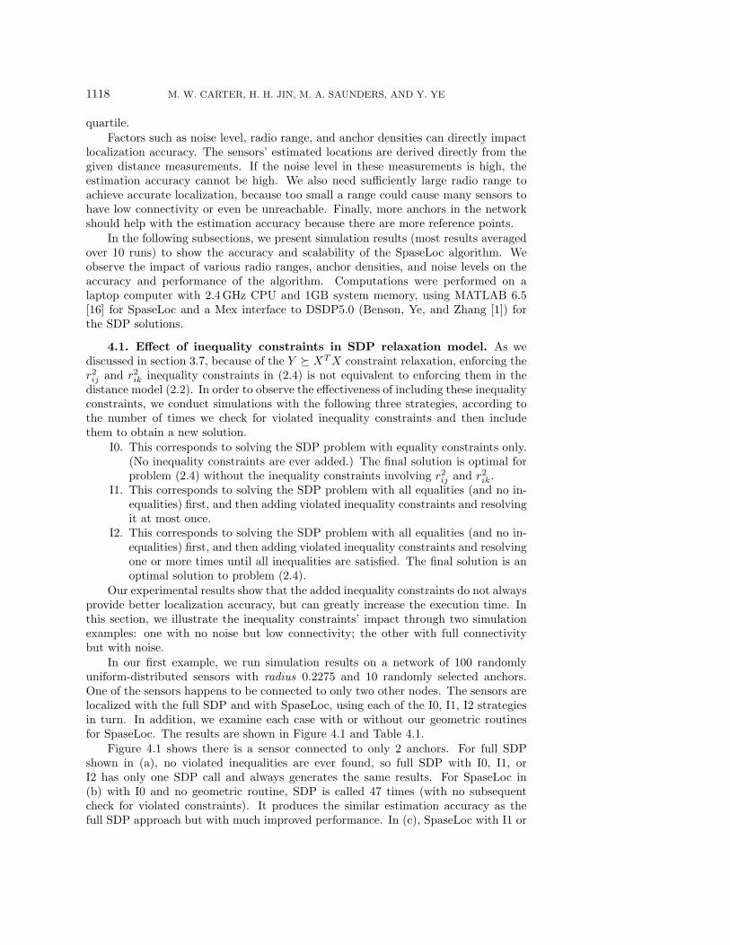
Factors such as noise level, radio range, and anchor densities can directly impactlocalization accuracy. The sensors’ estimated locations are derived directly from thegiven distance measurements. If the noise level in these measurements is high, theestimation accuracy cannot be high. We also need sufficiently large radio range toachieve accurate localization, because too small a range could cause many sensors tohave low connectivity or even be unreachable. Finally, more anchors in the networkshould help with the estimation accuracy because there are more reference points.

In the following subsections, we present simulation results (most results averagedover 10 runs) to show the accuracy and scalability of the SpaseLoc algorithm. Weobserve the impact of various radio ranges, anchor densities, and noise levels on theaccuracy and performance of the algorithm. Computations were performed on alaptop computer with 2.4 GHz CPU and 1GB system memory, using MATLAB 6.5[16] for SpaseLoc and a Mex interface to DSDP5.0 (Benson, Ye, and Zhang [1]) forthe SDP solutions.

4.1. Effect of inequality constraints in SDP relaxation model. As wediscussed in section 3.7, because of the Y XTX constraint relaxation, enforcing ther2ij and r2

ik inequality constraints in (2.4) is not equivalent to enforcing them in thedistance model (2.2). In order to observe the effectiveness of including these inequalityconstraints, we conduct simulations with the following three strategies, according tothe number of times we check for violated inequality constraints and then includethem to obtain a new solution.

I0. This corresponds to solving the SDP problem with equality constraints only.(No inequality constraints are ever added.) The final solution is optimal forproblem (2.4) without the inequality constraints involving r2

ij and r2ik.

I1. This corresponds to solving the SDP problem with all equalities (and no in-equalities) first, and then adding violated inequality constraints and resolvingit at most once.

I2. This corresponds to solving the SDP problem with all equalities (and no in-equalities) first, and then adding violated inequality constraints and resolvingone or more times until all inequalities are satisfied. The final solution is anoptimal solution to problem (2.4).

Our experimental results show that the added inequality constraints do not alwaysprovide better localization accuracy, but can greatly increase the execution time. Inthis section, we illustrate the inequality constraints’ impact through two simulationexamples: one with no noise but low connectivity; the other with full connectivitybut with noise.

In our first example, we run simulation results on a network of 100 randomlyuniform-distributed sensors with radius 0.2275 and 10 randomly selected anchors.One of the sensors happens to be connected to only two other nodes. The sensors arelocalized with the full SDP and with SpaseLoc, using each of the I0, I1, I2 strategiesin turn. In addition, we examine each case with or without our geometric routinesfor SpaseLoc. The results are shown in Figure 4.1 and Table 4.1.

Figure 4.1 shows there is a sensor connected to only 2 anchors. For full SDPshown in (a), no violated inequalities are ever found, so full SDP with I0, I1, orI2 has only one SDP call and always generates the same results. For SpaseLoc in(b) with I0 and no geometric routine, SDP is called 47 times (with no subsequentcheck for violated constraints). It produces the similar estimation accuracy as thefull SDP approach but with much improved performance. In (c), SpaseLoc with I1 or


−0.5 −0.4 −0.3 −0.2 −0.1 0 0.1 0.2 0.3 0.4 0.5−0.5

−0.4

−0.3

−0.2

−0.1

0

0.1

0.2

0.3

0.4

0.5

x

y

Full SDP with I0, I1, or I2

−0.5 −0.4 −0.3 −0.2 −0.1 0 0.1 0.2 0.3 0.4 0.5−0.5

−0.4

−0.3

−0.2

−0.1

0

0.1

0.2

0.3

0.4

0.5

x

y

SpaseLoc with I0 and no geometric routines

(a) (b)

−0.5 −0.4 −0.3 −0.2 −0.1 0 0.1 0.2 0.3 0.4 0.5−0.5

−0.4

−0.3

−0.2

−0.1

0

0.1

0.2

0.3

0.4

0.5

x

y

SpaseLoc with I1, or I2 and no geometric routines

−0.5 −0.4 −0.3 −0.2 −0.1 0 0.1 0.2 0.3 0.4 0.5−0.5

−0.4

−0.3

−0.2

−0.1

0

0.1

0.2

0.3

0.4

0.5

x

y

SpaseLoc with I0 and geometric routines

anchor positiontrue positionestimated positionerrors

(c) (d)

Fig. 4.1. Inequality impact on accuracy: 100 nodes, 10 anchors, no noise, radius 0.2275.

Table 4.1

Inequality impact on accuracy and speed: 100 nodes, 10 anchors, no noise, radius 0.2275.

Methods Error 95% Error Time SDP’sFull SDP with I0 or I1 or I2 1.7877e-3 1.7483e-10 11.97 1SpaseLoc with I0 and no geometric routines 1.7890e-3 1.1684e-7 0.38 47SpaseLoc with I1 or I2 and no geometric routines 1.7134e-3 1.1684e-7 0.42 48SpaseLoc with I0 and geometric routines 1.4679e-7 1.1523e-7 0.35 46

I2 produces the same results, which means violated inequalities are found only once.Comparing (b) and (c), we see that including violated inequalities does improve theestimation accuracy a little. Best of all in (d), SpaseLoc with I0 and our geometricroutines localizes all sensors with virtually no error.

Table 4.1 shows that adding violated inequalities increases execution time slightlyfor SpaseLoc.

In our second example, in order to observe the effectiveness of the inequalityconstraints under noise conditions, we run simulations for a network of 100 nodeswhose true locations are at the vertices of an equilateral triangle grid. Ten anchorsare placed at the middle grid-point of each row, and the radius is 0.25. A noise factor


−0.2 0 0.2 0.4 0.6 0.8 1 1.2−0.2

0

0.2

0.4

0.6

0.8

1

x

y

Full SDP with no inequalities

−0.2 0 0.2 0.4 0.6 0.8 1 1.2−0.2

0

0.2

0.4

0.6

0.8

1

x

y

Full SDP with all violated inequalities

(a) (b)

−0.2 0 0.2 0.4 0.6 0.8 1 1.2−0.2

0

0.2

0.4

0.6

0.8

1

x

y

SpaseLoc with no inequalities

−0.2 0 0.2 0.4 0.6 0.8 1 1.2−0.2

0

0.2

0.4

0.6

0.8

1

x

y

SpaseLoc with all violated inequalities


(c) (d)

Fig. 4.2. Inequality impact on accuracy: 100 nodes, 10 anchors, noise factor 0.1, radius 0.25.

Table 4.2

Inequality impact on accuracy and speed: 100 nodes, 10 anchors, noise factor 0.1, radius 0.25.

Methods Error Time SDP’sFull SDP with I0 0.1268 13.87 1Full SDP with I1 0.1292 34.20 2Full SDP with I2 0.1403 134.50 4SpaseLoc with I0 0.0231 0.45 54

SpaseLoc with I1 or I2 0.0203 0.51 56

of 0.1 is applied to the distance measurements. The sensors are localized with eitherfull SDP or SpaseLoc using I0, I1, I2 in turn without geometric routines. (Althoughwe do not activate the geometric routines in this experiment, they are not a factorhere because the localization error is not caused by low connectivity but by the noisymeasurements.) The results are shown in Figure 4.2 and Table 4.2. Figure 4.2(b) and(d) correspond to strategy I1 or I2 for full SDP and SpaseLoc.

As we can see, adding violated inequalities for full SDP not only increases theexecution times dramatically, but also increases the localization error. For SpaseLoc,adding violated inequalities improves the estimation accuracy slightly. Note that I1


and I2 produce the same results for SpaseLoc.In summary, the first experiment shows that when the errors are caused by low

connectivity, SpaseLoc with geometric routines and no inequality constraints (I0) out-performs SpaseLoc with inequalities (I1 or I2) and all of the full SDP options. Giventhis observation, from now on we only use SpaseLoc with geometric routines, whichmeans the geometric routines are used instead of SDP to localize sensors connectedto less than 3 anchors.

The second experiment indicates that under noise conditions, although addingviolated inequalities does not seem to improve the estimation accuracy for full SDP,it does improve accuracy for SpaseLoc.

In the subsequent sections, we continue to examine the inequality constraints’effects on accuracy and speed.

4.2. Accuracy and speed comparison: Full SDP versus SpaseLoc. Forvery small networks, the SDP approach is both accurate and efficient. (This is vitalto SpaseLoc, as many small subproblems must be solved using SDP.) However, theperformance of the full SDP approach deteriorates rapidly with network size.

Table 4.3 shows the localization results using full SDP (a) and using SpaseLoc(b) for a range of examples with various numbers of nodes whose true locations inthe network are at the vertices of an equilateral triangle grid. Anchors are placed atthe middle grid-point of each row. A noise factor of 0.1 is applied to the distancemeasurements.

Let us first look at the impact of I0, I1, and I2 on estimation accuracy. Table 4.3(a) shows that for full SDP, 8 errors with I1 are bigger than with I2, and 5 errorswith I2 are bigger than with I1. Comparing I0 with I2, we see that for each strategy,9 errors in I0 are bigger than the errors for the other strategy. It appears that fullSDP with added inequalities does not always improve the estimation accuracy. ForSpaseLoc, I1 and I2 generate almost equivalent estimation accuracy; I0 has 8 errorsthat are bigger than with I1, while I1 has 5 errors bigger than with I0. Therefore, theadded inequalities provide only marginal accuracy improvement for SpaseLoc.

Now let us compare full SDP with SpaseLoc. Figures 4.3–4.4 plot results forfull SDP with I0 and SpaseLoc with I0 for two of these examples: 9 and 49 nodes,including 3 and 7 anchors placed at the grid-point in the middle of each row. Aswe can see from these two figures and Table 4.3, for localizing 4 and 9 nodes, fullSDP and SpaseLoc show comparable performance. Beyond that size, the contrastgrows rapidly. For localizing 49 nodes, SpaseLoc is 10 times faster than the full SDPmethod, with more than four times the accuracy. For 400 nodes, SpaseLoc withstrategies I0, I1, and I2 is, respectively, 800, 2500, and 8500 times faster than fullSDP with the same strategies, while achieving 10 times greater accuracy. Thus, thefull SDP model becomes less effective as problem size increases. In fact, for problemsizes above 49 nodes, the average estimation error using full SDP becomes so largethat the computed solution is of little value.

It may seem nonintuitive that SpaseLoc’s greedy approach could produce smallererrors than the full SDP method. However, all of the SDP problems and subproblemsof the form (2.4) are relaxations of Euclidean models of the form (2.2). As we discussedin section 3.9, SpaseLoc always tries to create a subproblem whose subsensors havethree independent anchor connections, so that the SDP solution is exact. The sameconclusion cannot be drawn under noise conditions, but experimentally the relaxationsunder noise conditions appear to be tighter in SpaseLoc’s subproblems than in thesingle large SDP.


Table 4.3

Accuracy and speed comparison between full SDP and SpaseLoc.

(a) Full SDP

Number Radio Error Time (sec) SDP callsof nodes range I0 I1 I2 I0 I1 I2 I0 I1 I2

4 2.24 0.0317 0.0317 0.0317 0.01 0.01 0.01 1 1 19 1.12 0.1267 0.1203 0.1203 0.02 0.05 0.05 1 2 2

16 0.75 0.0837 0.0703 0.0680 0.10 0.21 0.35 1 2 325 0.56 0.0938 0.1170 0.1170 0.37 0.80 1.26 1 2 336 0.45 0.0719 0.0618 0.0561 0.81 1.88 3.02 1 2 349 0.40 0.1190 0.1190 0.1190 2.10 5.33 5.33 1 2 264 0.40 0.1218 0.0919 0.0954 3.43 9.21 21.60 1 2 481 0.40 0.1380 0.0894 0.0885 7.26 19.66 59.05 1 2 5

100 0.25 0.1268 0.1292 0.1403 13.87 34.20 140.26 1 2 4121 0.40 0.1157 0.1088 0.1091 23.24 81.62 182.74 1 2 3144 0.21 0.1480 0.1899 0.1891 37.76 168.43 584.23 1 2 4169 0.40 0.1283 0.1141 0.1217 71.87 278.72 692.12 1 2 4196 0.18 0.1404 0.1275 0.1286 151.52 461.97 1081.35 1 2 4225 0.40 0.1568 0.1589 0.1571 232.31 752.75 2408.67 1 2 5256 0.15 0.1429 0.1375 0.1370 356.86 1089.52 3260.33 1 2 5324 0.14 0.1685 0.1685 0.1685 962.66 2620.20 2620.20 1 2 2361 0.13 0.1734 0.1842 0.1833 1391.04 5051.05 15281.26 1 2 4400 0.12 0.1819 0.1970 0.1968 1662.22 5950.34 20321.60 1 2 4

(b) SpaseLoc

Number Radio Error Time (sec) SDP callsof nodes range I0 I1 I2 I0 I1 I2 I0 I1 I2

4 2.24 0.0317 0.0317 0.0317 0.02 0.02 0.02 1 1 19 1.12 0.0513 0.0513 0.0513 0.04 0.04 0.04 6 6 6

16 0.75 0.0615 0.0559 0.0559 0.06 0.19 0.09 8 9 925 0.56 0.0597 0.0608 0.0608 0.13 0.13 0.13 12 13 1336 0.45 0.0364 0.0294 0.0294 0.17 0.20 0.20 20 23 2349 0.40 0.0252 0.0252 0.0252 0.21 0.21 0.21 26 26 2664 0.40 0.0272 0.0273 0.0273 0.30 0.34 0.34 38 42 4281 0.40 0.0286 0.0295 0.0295 0.37 0.41 0.41 49 53 53

100 0.25 0.0232 0.0203 0.0203 0.46 0.49 0.49 54 56 56121 0.40 0.0238 0.0227 0.0227 0.57 0.61 0.61 74 77 77144 0.21 0.0230 0.0237 0.0237 0.69 0.70 0.70 84 89 89169 0.40 0.0200 0.0190 0.0190 0.80 0.84 0.84 100 106 106196 0.18 0.0177 0.0177 0.0177 0.98 1.08 1.08 84 90 90225 0.40 0.0226 0.0207 0.0208 1.07 1.41 1.47 94 109 110256 0.15 0.0208 0.0235 0.0249 1.21 1.44 1.50 118 131 132324 0.14 0.0179 0.0178 0.0178 1.64 1.70 1.70 157 158 158361 0.13 0.0218 0.0217 0.0217 1.89 2.01 2.01 177 181 181400 0.12 0.0176 0.0175 0.0175 2.02 2.37 2.37 184 201 201

In the following sections, we run more simulations only with SpaseLoc.

4.3. Scalability. Table 4.4 shows simulation results for 49 to 10000 randomlyuniform-distributed sensors being localized using SpaseLoc with strategies I0, I1, andI2. The node numbers 49, 100, 225, . . . are squares k2, and the radius is the minimumvalue that permits localization on a regular k×k grid. The number of anchors changeswith the number of sensors and is chosen to be k. Noise is not included in thissimulation. When the items under I1, I2 are empty, it means that they are equal tothe values under I0 in the same row.


0 0.2 0.4 0.6 0.8 1 1.2 1.4−0.2

0

0.2

0.4

0.6

0.8

1

1.2

x

y

Full SDP

−0.2 0 0.2 0.4 0.6 0.8 1 1.2 1.4−0.2

0

0.2

0.4

0.6

0.8

1

x

y

SpaseLoc


Fig. 4.3. 9 nodes on equilateral-triangle grids, 3 anchors, 0.1 noise, radius 1.12.

−0.2 0 0.2 0.4 0.6 0.8 1 1.2−0.2

0

0.2

0.4

0.6

0.8

1

x

y

Full SDP

−0.2 0 0.2 0.4 0.6 0.8 1 1.2 1.4−0.2

0

0.2

0.4

0.6

0.8

1

x

y

SpaseLoc


Fig. 4.4. 49 nodes on equilateral-triangle grids, 7 anchors, 0.1 noise, radius 0.40.

Table 4.4

SpaseLoc scalability. Strategies I1 and I2 generate same results.

Nodes An Ra Sub- Error 95% Error Time SDP’schors dius size I0 I1,I2 I0,I1,I2 I0 I1,I2 I0 I1,I2

49 7 0.3412 3 4.5840e-8 3.4449e-8 0.18 18100 10 0.2275 3 1.4679e-7 1.1523e-7 0.35 46225 15 0.1462 3 4.4940e-7 3.1248e-7 0.82 112529 23 0.0931 3 2.1662e-6 8.9873e-7 2.02 278

1089 33 0.0620 3 1.1969e-4 7.1510e-5 4.48 5872025 45 0.0451 4 1.4917e-4 1.4115e-4 9.6639e-5 8.85 9.28 1006 10073969 63 0.0334 4 1.2399e-4 7.2414e-5 18.79 18675041 71 0.0319 6 1.5172e-4 1.1918e-4 27.19 22106084 78 0.0290 6 1.7126e-4 1.1475e-4 33.66 27427056 84 0.0269 7 5.2369e-5 4.0388e-5 40.59 31178100 90 0.0251 7 2.7376e-4 2.7353e-4 1.7071e-4 47.87 49.71 3564 35669025 95 0.0238 7 2.1141e-4 2.1977e-4 1.6039e-4 54.41 56.03 3957 3958

10000 100 0.0226 7 2.0269e-4 1.5836e-4 59.33 4452

We find that strategies I1 and I2 produce the same results, and I0 gives essen-tially the same. This is because the inaccuracy of the estimation is caused purely bylow connectivity, not by noisy distance measurements. Empirically we see that theprogram scales well: almost linearly in the number of nodes in the network. Indeed,the computational complexity of the SpaseLoc algorithm is of order n, the number of


0 50 100 150 200 250 300 350 4000

200

400

600

800

1000

1200

1400

1600

1800

2000

n

tim

e

Full SDP times

SDP dataQuadraticCubicQuartic

Fig. 4.5. SDP computational complexity.

sensors in the network, even though the full SDP approach has much greater com-plexity, as we now show.

We know that in the full SDP model (2.4), the number of constraints is O(n2), andin each iteration of its interior-point algorithm the SDP solver needs to solve a sparselinear system of equations whose dimension is the number of constraints. Figure 4.5plots the CPU time for strategy I0 from Table 4.3(a) as well as three curves of theform time = apn

p for p = 2, 3, 4, where ap is determined by a least-squares fit. Itappears that the SDP complexity with strategy I0 lies somewhere between O(n3) andO(n4).

In SpaseLoc, we partition the full problem into p subproblems of size q or less,where p × q = n. We generally set q to be much smaller than n, ranging from 2 toaround 10 in most of our simulations. If t represents the execution time taken by thefull SDP method for a 10-node network, in the worst case the computation time forSpaseLoc is t × O(p). Thus, SpaseLoc is really linear in p in theory. Since we canassume q to be a parameter ranging from 2 to 10, with worst case 2, we know thatO(p) = O(n/q) ≤ O(n/2) = O(n). Now we can see that SpaseLoc’s computation timeis O(n).

In the remaining subsections we choose the middle network size from Table 4.4(nodes = 3969) to observe the effect of varying radio range, number of anchors, andnoise.

4.4. Radio range impact. With a fixed total number of randomly uniform-distributed nodes (3969, of which 63 are anchors), Table 4.5 shows the direct impactof radius in the range 0.0304 to 0.0334 on accuracy and performance.

Strategies I1 and I2 produce essentially the same results, and with slightly betteraccuracy than I0 for 8 of the 16 radius values, while I0 produces slightly betteraccuracy than I1 or I2 in 4 cases. However, I1 and I2 take more time than I0 becausethey need more SDP calls.


Table 4.5

Radio range impact: nodes = 3969, anchors = 63, no noise, sub size = 5.

rad- Error 95% Error Time SDP’sius I0 I1 I2 I0 I1 I2 I0 I1 I2 I0 I1 I2

0.0304 2.444e-3 2.359e-3 2.359e-3 4.035e-4 5.757e-4 5.757e-4 18.03 18.60 18.60 1743 1688 16890.0306 1.122e-3 1.123e-3 1.123e-3 5.638e-4 5.644e-4 5.644e-4 18.13 18.70 18.70 1747 1749 17490.0308 2.460e-3 1.412e-3 1.412e-3 7.952e-4 6.039e-4 6.039e-4 18.64 19.39 19.51 1879 1895 18960.0310 1.087e-3 1.083e-3 1.083e-3 4.424e-4 4.397e-4 4.397e-4 18.39 19.05 19.05 1809 1814 18140.0312 2.480e-3 2.481e-3 2.481e-3 3.142e-4 3.146e-4 3.146e-4 18.30 18.93 18.93 1715 1717 17170.0314 5.464e-4 5.337e-4 5.337e-4 2.612e-4 2.612e-4 2.612e-4 18.90 19.53 19.53 1897 1900 19000.0316 4.828e-4 4.827e-4 4.827e-4 2.645e-4 2.645e-4 2.645e-4 18.95 19.54 19.54 1916 1917 19170.0318 3.018e-4 3.013e-4 3.013e-4 1.955e-4 1.955e-4 1.955e-4 19.06 19.65 19.65 1911 1913 19130.0320 4.214e-4 4.214e-4 4.214e-4 1.781e-4 1.781e-4 1.781e-4 18.91 19.49 19.49 1847 1848 18480.0322 2.842e-4 2.842e-4 2.842e-4 1.702e-4 1.702e-4 1.702e-4 18.89 19.45 19.45 1894 1895 18950.0324 5.213e-4 5.495e-4 5.495e-4 2.968e-4 3.020e-4 3.020e-4 18.91 19.58 19.71 1859 1865 18660.0326 4.091e-4 4.033e-4 4.033e-4 2.323e-4 2.315e-4 2.315e-4 18.96 19.51 19.51 1890 1893 18930.0328 2.299e-4 2.289e-4 2.289e-4 1.363e-4 1.363e-4 1.363e-4 18.87 19.46 19.46 1921 1922 19220.0330 2.057e-4 2.160e-4 2.161e-4 9.435e-5 9.450e-5 9.450e-5 18.83 19.52 19.64 1873 1875 18760.0332 6.192e-4 6.439e-4 6.439e-4 3.557e-4 3.557e-4 3.557e-4 19.37 20.04 20.04 1849 1853 18530.0334 1.240e-4 1.240e-4 1.240e-4 7.241e-5 7.241e-5 7.241e-5 18.79 18.79 18.79 1867 1867 1867

Table 4.6

Number of anchors impact: nodes = 3969, radius = 0.0334, no noise, sub size = 5.

Anchors Error 95% Error Time SDP’sI0 I1,I2 I0 I1,I2 I0 I1,I2 I0 I1,I2

40 1.052e-3 1.052e-3 8.408e-4 8.409e-4 19.30 19.88 1906 190850 1.109e-3 1.128e-3 7.748e-4 7.745e-4 19.38 20.15 1861 1865

100 8.782e-4 7.280e-4 5.337e-4 5.115e-4 19.16 19.96 1870 1872150 2.716e-4 2.717e-4 1.025e-4 1.025e-4 18.86 19.60 1806 1808200 4.889e-5 4.872e-5 1.473e-5 1.473e-5 18.77 19.52 1795 1796250 1.716e-5 1.699e-5 7.760e-6 7.760e-6 18.55 19.32 1748 1749300 1.538e-5 1.521e-5 4.408e-6 4.408e-6 18.20 18.99 1750 1751350 7.533e-6 7.365e-6 2.858e-6 2.858e-6 18.13 18.93 1684 1685400 6.383e-6 6.215e-6 1.841e-6 1.841e-6 18.16 18.96 1560 1591

As we see, increasing radius leads to increased accuracy and only slightly morecomputational time. The simulation could assist sensor network designers in select-ing a radio range to achieve a desired estimation accuracy with little concern aboutalgorithm speed.

4.5. Number of anchors impact. With constant radius (0.0334) and the samerandomly distributed nodes (3969), Table 4.6 shows the impact of the number ofanchors, ranging from 1% to 10% of the total number of points. (Noise is not included.)

Strategies I1 and I2 produce identical results. Comparing I0 with I1 or I2, wesee that added inequalities slightly improve the average error consistently, althoughthe 95% error remains essentially the same. Increasing the number of anchors inthe network improves the estimation accuracy in general, with no obvious impact onalgorithm speed. However, we don’t see accuracy improvement when the number ofanchors reaches more than 10% of the total points. This analysis is beneficial fordesigners to avoid the cost of deploying unnecessary anchors.

4.6. Noise impact. With constant radius (0.0334) and the same randomly dis-tributed nodes (3969), Table 4.7 shows the impact of noise conditions on accuracyand performance.

We see that strategies I1 and I2 do not provide consistent improvement over I0 forboth average and 95% error, yet they always increase execution time. Also, more noisein the network has a direct impact on estimation accuracy. Simulations of this kindmay help designers determine the measurement noise level that will give an acceptableestimation error.


Table 4.7

Noise factor impact: nodes = 3969, anchors = 400, radius = 0.0334, sub size = 5.

Noise Error 95% Error Time SDP’sfactor I0 I1 I2 I0 I1 I2 I0 I1 I2 I0 I1 I20.01 9.60e-4 9.59e-4 9.59e-4 1.90e-6 3.16e-4 3.16e-4 20.38 21.18 21.20 1622 1623 16230.05 3.15e-3 8.33e-3 8.33e-3 3.16e-4 3.57e-3 3.57e-3 21.56 21.75 21.86 1479 1253 12560.10 6.87e-3 7.36e-3 1.03e-2 1.91e-3 5.17e-3 6.95e-3 21.46 24.73 22.94 1447 1592 12300.20 1.55e-2 1.57e-2 1.65e-2 4.95e-3 1.16e-2 1.25e-2 21.55 25.67 25.83 1208 1433 13900.30 1.51e-2 1.48e-2 1.46e-2 1.17e-2 1.27e-2 1.24e-2 21.09 29.76 31.78 1411 1829 18440.40 1.98e-2 1.79e-2 1.79e-2 1.32e-2 1.57e-2 1.57e-2 21.30 32.05 35.15 1523 1985 20730.50 3.05e-2 2.35e-2 2.28e-2 2.86e-2 2.16e-2 2.08e-2 22.07 35.27 39.26 1608 2157 2252

5. Summary and extensions. We have shown that SpaseLoc achieves the aimsof accuracy, speed, and scalability with a single processor on very large networks. Ittakes full advantage of the recent SDP approach of Biswas and Ye [2]. The latter hascomputational complexity O(np), where n is the network size and p is between 3 and4, but we use it on multiple tiny subproblems to obtain an algorithm with essentiallylinear complexity. On a 2.4GHz laptop with 1GB memory, SpaseLoc maintains effi-ciency and provides accurate location estimation for networks with 10000 sensors andbeyond.

0 50 100 150 200 250 300 350 4000

0.02

0.04

0.06

0.08

0.1

0.12

0.14

0.16

0.18

0.2

Sensors in network

Me

an

loca

liza

tion

err

or

SDP errorsSpaseLoc errors

0 1000 2000 3000 4000 5000 6000 7000 8000 9000 100000

10

20

30

40

50

60

70

Sensors in network

CP

U s

econ

ds

SDP timeSpaseLoc time

Fig. 5.1. Accuracy and performance comparison.

Figure 5.1 compares localization results for our SpaseLoc algorithm and the fullSDP approach [2] for various sized networks. The left-hand figure shows a comparisonin terms of estimation accuracy for localizing various sizes of networks when sensorsare placed at the vertices of an equilateral triangle grid with 0.1 noise factor added todistance measurements (data is taken from Table 4.3). It shows clearly that SpaseLocprovides much improved localization accuracy.

The right-hand graph summarizes results in terms of execution time on variousnetwork sizes. Data for the full SDP method is taken from Table 4.3, and data forSpaseLoc is taken from Table 4.4. The figure confirms near-linear complexity forSpaseLoc.

5.1. More general problems. In Jin [14], SpaseLoc is used as a building blockfor more general localization algorithms. A dynamic version can estimate movingsensors’ locations in real time, and a three-dimensional version extends its utilityfurther. For clustered and distributed environments, it is shown how to use SpaseLoc


in parallel (on multiple large subproblems) to obtain essentially linear complexity onclustered networks of unlimited size. Finally, a preprocessor for SpaseLoc has beendeveloped in [14] to localize sensors in anchorless networks.

5.2. A bootstrap procedure. SpaseLoc works effectively when Step A1 (sub-problem creation) finds subsensors connected to at least 3 anchors. A difficult situa-tion arises if there are more than 3 anchors in the network but no subsensor is directlyconnected to 3 anchors. A network with anchors placed at the borders of the regionis such an example. SpaseLoc’s subproblems will involve sensors connected to only 2or 1 anchors, leading to a less accurate final solution.

When there is sufficient connection information for sensors to be indirectly con-nected to at least 3 anchors through other sensors, the full SDP approach can find asolution. We are developing a procedure to choose a subproblem in the above situa-tion. It will include the anchors, certain subsensors, and the sensors on each shortestpath from a subsensor to an anchor.

5.3. Alternative subproblem solvers. At present, most of the SpaseLoc sub-problems are solved by the SDP approach of Biswas and Ye [2]. This is an approxima-tion method that may produce large errors with noisy data. A recent development byBiswas et al. [4] adds regularization terms to the SDP problem and uses a gradient-descent method to refine the SDP solution. Significant accuracy improvement isreported. An advantage of SpaseLoc is that it can solve each subproblem by anymethod that is effective on small networks. Our next step is to experiment with suchapproaches, including that of [4] and various triangulation-based methods.

Acknowledgments. We gratefully acknowledge valuable technical advice fromProfs. Henry Wolkowicz, Scott Rogers, and Daniel Frances and two perceptive referees.Thanks also to Dr. Steve Benson for his expert advice on using the DSDP5.0 solverand to Prof. Kenneth Holmstrom for his help in fine-tuning parts of the MATLABimplementation of SpaseLoc. We are further indebted to Robert Bosch Corporationand the talented Bosch RTC team: Sharmila Ravula, Lakshmi Venkatraman, BhaskarSrinivasan, Abtin Keshavarzian, Hauke Schmidt, and Karsten Funk; they providedthe inspiration and vision for our algorithms to be practical.

REFERENCES

[1] S. J. Benson, Y. Ye, and X. Zhang, DSDP Website, http://www-unix.mcs.anl.gov/˜bensonor http://www.stanford.edu/˜yyye/Col.html (1998–2005).

[2] P. Biswas and Y. Ye, Semidefinite programming for ad hoc wireless sensor network localiza-tion, in Proceedings of the Third International Symposium on Information Processing inSensor Networks, Berkeley, CA, 2004.

[3] P. Biswas and Y. Ye, A distributed method for solving semidefinite programs arising from adhoc wireless sensor network localization, in Multiscale Optimization Methods and Appli-cations, Nonconvex Optim. Appl. 82, Springer, New York, 2006.

[4] P. Biswas, T. Liang, K. Toh, T. Wang, and Y. Ye, Semidefinite programming approaches forsensor network localization with noisy distance measurements, IEEE Trans. AutomationSci. Engrg., to appear.

[5] S. Boyd, L. El Ghaoui, E. Feron, and V. Balakrishnan, Linear Matrix Inequalities inSystem and Control Theory, SIAM Stud. Appl. Math. 15, SIAM, Philadelphia, 1994.

[6] N. Bulusu, J. Heidemann, and D. Estrin, GPS-less Low Cost Outdoor Localization forVery Small Devices, Technical report 00-729, Computer Science Department, Universityof Southern California, Los Angeles, CA, 2000.

[7] D. Culler and W. Hong, Wireless sensor networks, Comm. ACM, 47 (2004), pp. 30–33.[8] L. Doherty, L. El Ghaoui, and K. Pister, Convex position estimation in wireless sensor

networks, in Proceedings of the IEEE Infocom 2001, Anchorage, AK, 2001, pp. 1655–1663.[9] A. Dragoon, Small wonders, CIO Magazine, January 15, 2005.


[10] D. Ganesan, B. Krishnamachari, A. Woo, D. Culler, D. Estrin, and S. Wicker, An Em-pirical Study of Epidemic Algorithms in Large-Scale Multihop Wireless Networks, ReportUCLA/CSD-TR-02-0013, Computer Science Department, University of California at LosAngeles, Los Angeles, CA, 2002.

[11] G. H. Golub and C. F. Van Loan, Matrix Computations, 3rd ed., The Johns Hopkins Uni-versity Press, Baltimore, 1996.

[12] J. Hightower and G. Boriello, Location systems for ubiquitous computing, IEEE Computer,34 (2001), pp. 57–66.

[13] A. Howard, M. J. Mataric, and G. S. Sukhatme, Relaxation on a mesh: A formalismfor generalized localization, in Proceedings of the IEEE/RSJ International Conference onIntelligent Robots and Systems (IROS01), Maui, HI, 2001, pp. 1055–1060.

[14] H. H. Jin, Scalable Sensor Localization Algorithms for Wireless Sensor Networks, Ph.D. the-sis, University of Toronto, Toronto, Canada, 2005. (Joint research conducted at StanfordUniversity.)

[15] M. Lawlor, Small systems, big business, Signal Magazine, January 2005.[16] MATLAB 6.5, Release 13 with Service Pack 1, The MathWorks, Inc., Natick, MA, 2003.[17] D. Niculescu and B. Nath, Ad hoc positioning system, in Proceedings of the IEEE GlobeCom

2001, San Antonio, TX, 2001, pp. 2926–2931.[18] A. Ricadela, Sensors everywhere, Information Week, January 24, 2005.[19] C. Savarese, J. Rabaey, and K. Langendoen, Robust positioning algorithm for distributed ad

hoc wireless sensor networks, in Proceedings of the USENIX Technical Annual Conference,Monterey, CA, 2002.

[20] A. Savvides, C.-C. Han, and M. B. Srivastava, Dynamic fine-grained localization in ad hocnetworks of sensors, in Proceedings of the ACM/IEEE International Conference on MobileComputing and Networking (MOBICON), Rome, Italy, 2001, pp. 166–179.

[21] A. Savvides, H. Park, and M. B. Srivastava, The bits and flops of the n-hop multilaterationprimitive for node localization problems, in Proceedings of the 1st ACM InternationalWorkshop on Wireless Sensor Networks and Applications (WSNA’02), Atlanta, GA, ACMPress, New York, 2002, pp. 112–121.

[22] Y. Shang, W. Ruml, Y. Zhang, and M. Fromherz, Localization from mere connectivity, inProceedings of the Fourth ACM International Symposium on Mobile Ad Hoc Networkingand Computing, Annapolis, MD, ACM Press, New York, 2003, pp. 201–212.

[23] J. F. Sturm, Let SeDuMi Seduce You, http://fewcal.kub.nl/sturm/software/sedumi.html (Oc-tober 2001).

[24] R. Szewczyk, E. Osterweil, J. Polastre, M. Hamilton, A. Mainwaring, and D. Estrin,Habitat monitoring with sensor networks, Comm. ACM, 47 (2004), pp. 34–44.

[25] P. Tseng, SOCP relaxation for nonconvex optimization, presented at ICCOPT 1, RensselaerPolytechnic Institute, Troy, NY, 2004.

SPASELOC: AN ADAPTIVE SUBPROBLEM ALGORITHM FOR …

Documents

Transcript of SPASELOC: AN ADAPTIVE SUBPROBLEM ALGORITHM FOR …