sensors

Article

Sparse Reconstruction for Micro Defect Detection inAcoustic Micro Imaging

Yichun Zhang 1, Tielin Shi 1, Lei Su 2,*, Xiao Wang 1, Yuan Hong 1, Kepeng Chen 1 andGuanglan Liao 1,*

1 State Key Laboratory of Digital Manufacturing Equipment and Technology,Huazhong University of Science and Technology, Wuhan 430074, China;zhangyc@hust.edu.cn (Y.Z.); tlshi@hust.edu.cn (T.S.); wangxiao1989@hust.edu.cn (X.W.);hongyuan@hust.edu.cn (Y.H.); ckphust@hust.edu.cn (K.C.)

2 Jiangsu Key Laboratory of Advanced Food Manufacturing Equipment and Technology,Jiangnan University, Wuxi 214122, China

* Correspondence: lei_su2015@jiangnan.edu.cn (L.S.); guanglan.liao@hust.edu.cn (G.L.);Tel.: +86-510-8591-0562 (L.S.); +86-27-8779-3103 (G.L.)

Academic Editors: Dipen N. Sinha and Cristian PanteaReceived: 28 July 2016; Accepted: 12 October 2016; Published: 24 October 2016

Abstract: Acoustic micro imaging has been proven to be sufficiently sensitive for micro defectdetection. In this study, we propose a sparse reconstruction method for acoustic micro imaging.A finite element model with a micro defect is developed to emulate the physical scanning. Then weobtain the point spread function, a blur kernel for sparse reconstruction. We reconstruct deblurredimages from the oversampled C-scan images based on l1-norm regularization, which can enhancethe signal-to-noise ratio and improve the accuracy of micro defect detection. The method is furtherverified by experimental data. The results demonstrate that the sparse reconstruction is effective formicro defect detection in acoustic micro imaging.

Keywords: sparse reconstruction; micro defect; acoustic micro-imaging; point spread function

1. Introduction

The most commonly used methods in nondestructive evaluation for micro defect detectionare acoustic micro imaging (AMI), X-ray [1,2], and infrared thermography [3]. AMI, also knownas scanning acoustic microscopy, has been proven to be sufficiently sensitive for detecting microdefects and features, such as delamination [4,5], voids in the interfaces [6], microbubbles [7,8],stress distributions [9], solder bumps in flip chip [10,11], etc. The general working modes of AMIinclude A-scan, B-scan, and C-scan, obtaining time-domain signal, time-spatial image, and spatialimage, respectively.

Most investigations have focused on the A-scan signal [12–15] to improve the resolution ofultrasonic detection by separating the echoes via sparse reconstruction. The sparse reconstructionhas also been introduced to improve the resolution of B-scan image [16–18]. In these works, the sizeof the objects was up to a millimeter and the central frequency of the planar immersion transduceror contact transducer was only 5 MHz. Till now, little work has been involved in research on sparsereconstruction for C-scan images of AMI. Actually, C-scan can provide more effective results thanA/B-scan for detecting micro defects, and the transducer is a focusing transducer whose centralfrequency can be as high as 230 MHz [10,11] or even GHz [6]. The acoustic field distribution of thefocusing transducer is completely different from the planar transducer, and the formation of the C-scanimage is also different from that of the B-scan image. For C-scan mode, the key parameter of sparsereconstruction is the point spread function (PSF), also known as blur kernel in image processing.

Sensors 2016, 16, 1773; doi:10.3390/s16101773 www.mdpi.com/journal/sensors

Sensors 2016, 16, 1773 2 of 11

The PSF describes the response of a transducer system to a point source or reflector placed at thefocal plane. By scanning a small target in water, Canumalla obtained the PSF of the transducer withthe highest center frequency of 30 MHz [19]. However, the acoustic propagation within the solidspecimen is different from the condition that the target is directly immersed in the water. The PSFin the specimen should be different from the one in water. Moreover, the focal zone in the specimenof the high frequency transducer like 230 MHz only has a size of 10s of micrometers, and the targetfor measuring the PSF should be limited to a few micrometers. Besides, the PSF covered by noisecannot be obtained directly. It is hard to measure the PSF directly for high frequency transducer inAMI. Zhang et al. developed a 2D AMI finite element model of a flip-chip package to investigate theacoustic propagation inside the package [20–23], while sparse reconstruction and super resolutionwere not involved.

In this work, we propose a sparse reconstruction method for micro defect detection in AMI.A finite element model which contains a micro defect with unit size is developed. Then we shiftthe defect to emulate the scanning system, and acquire the PSF of the system. By using the PSF asa blur kernel, we reconstruct the deblurred image from the oversampled C-scan image based onl1-norm regularization, and improve the accuracy for micro defect detection successfully. The sparsereconstruction was further verified by experimental results, proving its effectiveness in improvingresolution and enhancing signal-to-noise ratio for micro defect detection.

2. Method

The AMI system working on C-scan is modeled as a linear time invariant (LTI) system,

y = k⊗ x + n (1)

where the output signal y denotes an observed C-scan image, k is a matrix representing the PSF of theAMI system, the input signal x (the reflectivity field) denotes an ideal C-scan image, n denotes thenoise, and ⊗ is convolution operation. When y is available and x needs to be estimated, the problem isan ill-posed problem where prior image information is required [24]. Considering that the defects inan object are generally finite and their distribution is sparse, only a few pixel values of the image xwhere the defect exists should be non-zero, and the others should be 0. Thus we can add an l1-normregularization term to make sure x be sparse, and obtain the reconstructed image x̂ by solving theoptimization problem,

x̂ = argminx

λ||k⊗ x− y||22 + ||x||1 (2)

where || ||2 denotes the Euclidean norm, || ||1 denotes the l1-norm in vector, and λ is theregularization parameter. The first term ensures that the solution is consistent with the observed image,and the second term inserts the image prior information to the solution. The problem in Equation (2) isa typical convex l1-regularized problem [24,25] that can be solved by iterative shrinkage-thresholdingalgorithm (ISTA) [26]. The regularization parameter λ balances the first term and second term ofEquation (2), which means the value is affected by the fidelity of the measurements, the noise level,and the sparse level of the image [26]. For a given C-scan image, a large value will result in a leastsquares solution which may be unstable, while a small value may over smooth the solution due toexcessive regularization [18,26–28]. Here, we set λ according to the method described in [28].

Then y and x̂ are evaluated using a target-to-clutter ratio (TCR) metric adapted from [28], which isa measure of the signal in the target region relative to the signal from the background region. The TCRrepresents the signal-to-noise ratio of the image,

TCR = 20log10

((

1NT

∑T

fij)/(1

Nb∑b

fij)

), (3)

Sensors 2016, 16, 1773 3 of 11

where fij denotes the pixel of the image, T denotes the target region in the image, NT is the numberof pixels in the target region, b denotes the background region, and Nb is the number of pixels in thebackground region. Due to the l1-norm regularization, most of the pixel values in the backgroundregion will be zero, and the signal-to-noise ratio can be significantly enhanced. We call this methodAMI sparse reconstruction (AMISR), whose pseudocode is presented in Algorithm 1. The parametersδ and ε, both set to 0.001, are the step sizes for ISTA update and convergence tolerance, respectively.The operator S is a soft shrinkage operation, defined as Sδ(xi) = max {|xi| − δ, 0} · sign(xi), shrinkingevery component of the input matrix towards zero.

Algorithm 1. Pseudocode of AMISR

1: Input: Oversampled C-scan image y, point spread function k, regularization parameters δ, ε, λ

2: Initialization x0 = y, flag = 13: while (flag), do4: υk = xk − δλKT(Kxk − y)5: xk+1 = Sδ(υk)

6: if ||xk+1 − xk||22 < ε

7: x̂ = xk+1, flag = 08: end9: end10: Calculate TCR11: Output: Reconstruct image x̂ , TCR

3. Point Spread Function (PSF)

3.1. Modeling

The PSF describes the response of the AMI system (with the spatial sampling intervals of 1 µm) toa defect (with the size of 1 µm) placed at the focal plane, i.e., the observed C-scan image. The finiteelement model is developed with the commercial software (COMSOL Multiphysics 5.2), as shownin Figure 1. To overcome the huge computational resource requirements [20–23], we design a virtualtransducer (VT) by reducing the size of the physical transducer (1/20 of the physical transducer) in themodel, as shown in Figure 1a. The sizes of the coupling water zone and the thickness of the sampleare also reduced. The arc that represents the VT has a chord length of 98.8 µm and a curvature radiusof 399.3 µm. The micro defect has a width of 1 µm and a height of 50 µm, as shown in Figure 1b.The material properties used in the model are obtained from the material library of the COMSOL.The acoustic velocities in water and tungsten are 1484 m/s and 4620 m/s, respectively. The densitiesof water and tungsten are set to 1000 Kg/m3 and 17,800 Kg/m3. The Poisson’s ratio and Young’smodulus of tungsten are 0.27 and 360 GPa. The ultrasonic excitation signal is a broadband modulatedpulse which can be modeled as a Gabor function,

f (t) = A · exp(−π(t− µ)2

σ2 ) · sin(2π f0t) (3)

where A is the reference amplitude, f 0 is the central frequency of the transducer (230 MHz), andµ = 2/f 0 and σ = 1/(2f 0) are the translation and standard deviation of Gaussion function. The Gaborfunction is defined as the normal displacement of the VT arc during excitation. After the excitation,the VT arc is set as a radiation boundary for receiving signals. The solid-liquid interface is set as anacoustic-structural coupled boundary, and the other boundaries are set as radiation boundaries inthe liquid region and low reflection boundaries in the solid region. The grid in the model is set as10 elements per wavelength. The temporal resolution is set as 25 time steps per period of the acoustic

Sensors 2016, 16, 1773 4 of 11

wave. The simulation is carried out for 90 ns, where the excitation lasts for the first 20 ns. The integralof the pressure data along the transducer arc is defined as the received signal of the VT.

We first carry out transient simulation in tungsten without defect to confirm the position of thefocus of the VT, as shown in Figure 1c. Afterwards, the defect is located in the focal plane of the VTwith the horizontal position changing at 1 µm intervals in simulations. Since the model is axisymmetric,only half of the model is scanned.

Sensors 2016, 16, 1773 4 of 11

with the horizontal position changing at 1 μm intervals in simulations. Since the model is

axisymmetric, only half of the model is scanned.

Figure 1. The simulation model (unit in μm ): (a) The geometrical model; (b) Area segments in the

model with defect; (c) Area segments in the model without defect; (d) Meshing with 10 elements per

wavelength, and the position of defect is offset to emulate the transducer scanning in AMI.

3.2. Characteristics of the VT

Figure 2a depicts the beam profile obtained from the model (Figure 1c) by mapping maximum

displacement of the coordinate points, where an obvious focus region can be observed. Figures 2b,c

indicates the normalized displacement along the dash lines labeled in Figure 2a. The red dash lines

indicating −6 dB cut-off threshold define the depth of field (DOF) and the spot size of the VT. The

spot size in tungsten is measured as 27 μm in Figure 2b. The DOF is given as 261 μm in Figure 2c

with the focal plane about −96 μm.

Figure 1. The simulation model (unit in µm ): (a) The geometrical model; (b) Area segments in themodel with defect; (c) Area segments in the model without defect; (d) Meshing with 10 elements perwavelength, and the position of defect is offset to emulate the transducer scanning in AMI.

3.2. Characteristics of the VT

Figure 2a depicts the beam profile obtained from the model (Figure 1c) by mapping maximumdisplacement of the coordinate points, where an obvious focus region can be observed. Figure 2b,cindicates the normalized displacement along the dash lines labeled in Figure 2a. The red dash linesindicating −6 dB cut-off threshold define the depth of field (DOF) and the spot size of the VT. The spotsize in tungsten is measured as 27 µm in Figure 2b. The DOF is given as 261 µm in Figure 2c with thefocal plane about −96 µm.

Sensors 2016, 16, 1773 5 of 11Sensors 2016, 16, 1773 5 of 11

Figure 2. Characteristics of the VT in solid (unit in μm): (a) Beam profile of the VT with diagram of

DOF and the spot size; (b) Spot size measurement in lateral direction; (c) Depth of field

measurement in vertical direction.

3.3. C-Scan and PSF

Figure 3a depicts a representative A-scan signal with the transducer at the position 0 μm,

which indicates that the transducer is located upon the center of the defect. The echo of the defect is

too weak compared with that of the surface, which is zoomed in the insert. The dash lines represent

the gate of echo. A-scans are then assembled in Figure 3b like a B-scan image, where only the echo

of the defect is shown. Every column of the figure represents an A-scan signal obtained in every

simulation with a different position of the defect, and every row represents the varied time of the

received signal. The defect echo gated by the dash lines is the received signal related to the defect.

Some interference signals are observed when the transducer is far away from the defect, which may

be caused by the sidelobe of the focus region as shown in Figure 2a.

The maximum amplitude values of the gated A-scan signals are calculated, forming the C-line

as displayed in Figure 3c. Obviously, it decreases when the transducer moves away from the defect.

The C-scan is produced after mapping the C-line around the central axis, as shown in Figure 3d. By

abandoning the small values caused by the interference signal, we acquire the PSF and normalize it

as illustrated in Figure 3e, which can be used for further analysis.

Figure 2. Characteristics of the VT in solid (unit in µm): (a) Beam profile of the VT with diagram ofDOF and the spot size; (b) Spot size measurement in lateral direction; (c) Depth of field measurementin vertical direction.

3.3. C-Scan and PSF

Figure 3a depicts a representative A-scan signal with the transducer at the position 0 µm, whichindicates that the transducer is located upon the center of the defect. The echo of the defect is tooweak compared with that of the surface, which is zoomed in the insert. The dash lines represent thegate of echo. A-scans are then assembled in Figure 3b like a B-scan image, where only the echo of thedefect is shown. Every column of the figure represents an A-scan signal obtained in every simulationwith a different position of the defect, and every row represents the varied time of the received signal.The defect echo gated by the dash lines is the received signal related to the defect. Some interferencesignals are observed when the transducer is far away from the defect, which may be caused by thesidelobe of the focus region as shown in Figure 2a.

The maximum amplitude values of the gated A-scan signals are calculated, forming the C-lineas displayed in Figure 3c. Obviously, it decreases when the transducer moves away from the defect.The C-scan is produced after mapping the C-line around the central axis, as shown in Figure 3d.By abandoning the small values caused by the interference signal, we acquire the PSF and normalize itas illustrated in Figure 3e, which can be used for further analysis.

Sensors 2016, 16, 1773 6 of 11Sensors 2016, 16, 1773 6 of 11

Figure 3. The A-scan, C-scan, and PSF (unit in μm): (a) A-scan of the model with the transducer at

position 0 μm; (b) B-scan like image; (c) C-line; (d) C-scan; (e) PSF extracted from (d).

4. Experimental Verification

Three samples with artificial defects (including single groove, two grooves, and a complex

defect) were used for verification. A circular tungsten sheet 4 inches in diameter and 500 μm in

thickness was polished to optical flatness on both sides. Then the defect pattern was etched with the

depth about 50 μm by inductive couple plasmas (ICP) etching. After that, the sheet was cut into

small pieces with the area about ~10 × 10 mm2. The AMI test was performed on the pieces using a

scanning acoustic microscopy (SAM, D9500, Sonoscan, Elk Grove Village, IL, USA), as shown in

Figure 4a. The transducer (230SP) had a central frequency of 230 MHz and a focal length of

7924.8 μm in water. The f-number of the transducer was 4. The pieces were immersed in water and

the focus of the transducer was located at the bottom of the artificial defects. The spatial sampling

interval of the scanning system was 1 μm for 1 pixel, in accord with the simulation. Finally, the

topography of the artificial defects was measured with a laser scanning confocal microscopy

(LSCM, VK-X200K, Keyence, Japan) for comparison.

4.1 Single Groove

Figure 4b displays the topography of the single groove obtained by LSCM, and the average

height of the region indicated by the black box is given in Figure 4c. The sidewall of the groove has

a slight tilt caused inevitably by the ICP process. To determine the bottom and the sidewall,

first-order derivative of the height curve is shown in the insert. The region where the derivative

almost equals zero is considered as the bottom, of which the width is 23.5 μm.

The original C-scan image and reconstructed image by the AMISR are presented in Figure 4d

and Figure 4e, respectively. To avoid the interference of the noise, the average profiles along the

direction of the groove are presented in dB (Figure 4f). The blue line and red line represent the

average profiles calculated from the blue block in Figure 4d and the red block in Figure 4e. Here the

−6 dB width is defined as the width of the groove. We obtain the width of 37.5 μm (according to the

original C-scan image) and 22 μm (according to the reconstructed image). Compared with the

width obtained from the LSCM, the AMISR provides a more accurate result (only 6.4% deviation)

than the original C-scan (59.6% deviation).

To quantify the image formed by the AMISR and C-scan, TCR is calculated to analyze the

signal-to-noise ratio. The cross section of the groove based on the reference values is generated as a

Figure 3. The A-scan, C-scan, and PSF (unit in µm): (a) A-scan of the model with the transducer atposition 0 µm; (b) B-scan like image; (c) C-line; (d) C-scan; (e) PSF extracted from (d).

4. Experimental Verification

Three samples with artificial defects (including single groove, two grooves, and a complex defect)were used for verification. A circular tungsten sheet 4 inches in diameter and 500 µm in thickness waspolished to optical flatness on both sides. Then the defect pattern was etched with the depth about50 µm by inductive couple plasmas (ICP) etching. After that, the sheet was cut into small pieces withthe area about ~10 × 10 mm2. The AMI test was performed on the pieces using a scanning acousticmicroscopy (SAM, D9500, Sonoscan, Elk Grove Village, IL, USA), as shown in Figure 4a. The transducer(230SP) had a central frequency of 230 MHz and a focal length of 7924.8 µm in water. The f-number ofthe transducer was 4. The pieces were immersed in water and the focus of the transducer was locatedat the bottom of the artificial defects. The spatial sampling interval of the scanning system was 1 µmfor 1 pixel, in accord with the simulation. Finally, the topography of the artificial defects was measuredwith a laser scanning confocal microscopy (LSCM, VK-X200K, Keyence, Japan) for comparison.

4.1. Single Groove

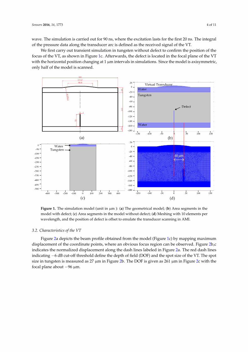
Figure 4b displays the topography of the single groove obtained by LSCM, and the average heightof the region indicated by the black box is given in Figure 4c. The sidewall of the groove has a slight tiltcaused inevitably by the ICP process. To determine the bottom and the sidewall, first-order derivativeof the height curve is shown in the insert. The region where the derivative almost equals zero isconsidered as the bottom, of which the width is 23.5 µm.

The original C-scan image and reconstructed image by the AMISR are presented in Figure 4d andFigure 4e, respectively. To avoid the interference of the noise, the average profiles along the directionof the groove are presented in dB (Figure 4f). The blue line and red line represent the average profilescalculated from the blue block in Figure 4d and the red block in Figure 4e. Here the −6 dB width isdefined as the width of the groove. We obtain the width of 37.5 µm (according to the original C-scanimage) and 22 µm (according to the reconstructed image). Compared with the width obtained fromthe LSCM, the AMISR provides a more accurate result (only 6.4% deviation) than the original C-scan(59.6% deviation).

Sensors 2016, 16, 1773 7 of 11

To quantify the image formed by the AMISR and C-scan, TCR is calculated to analyze thesignal-to-noise ratio. The cross section of the groove based on the reference values is generated as amask (illustrated in Figure 4g). To distinguish the target region from the background region, the maskis superimposed on the original C-scan image (Figure 4h) and the image formed by AMISR (Figure 4i).The TCR of the AMISR result is 41.8 dB, almost four times that of the original C-scan (10.5 dB). Hence,the proposed method can significantly enhance the signal-to-noise ratio.

Sensors 2016, 16, 1773 10 of 17

To quantify the image formed by the AMISR and C-scan, TCR is

calculated to analyze the signal-to-noise ratio. The cross section of the

groove based on the reference values is generated as a mask

(illustrated in Figure 4g). To distinguish the target region from the

background region, the mask is superimposed on the original C-scan

image (Figure 4h) and the image formed by AMISR (Figure 4i). The

TCR of the AMISR result is 41.8 dB, almost four times that of the

original C-scan (10.5 dB). Hence, the proposed method can

significantly enhance the signal-to-noise ratio.

Figure 4. Results of the single groove (unit in μm): (a) Schematic

diagram of AMI; (b) The topography of the groove; (c) Average

profile of the groove; (d) Original C-scan image; (e) The

reconstructed image formed by AMISR; (f) Average values of

the regions indicated in (d) and (e); (g) The cross section of the

groove; (h) The original C-scan image superimposed with the

mask; (i) The reconstructed image superimposed with the mask.

4.2 Two Grooves

Figure 4. Results of the single groove (unit in µm): (a) Schematic diagram of AMI; (b) The topographyof the groove; (c) Average profile of the groove; (d) Original C-scan image; (e) The reconstructed imageformed by AMISR; (f) Average values of the regions indicated in (d) and (e); (g) The cross section ofthe groove; (h) The original C-scan image superimposed with the mask; (i) The reconstructed imagesuperimposed with the mask.

4.2. Two Grooves

The topography of the two grooves obtained by the LSCM is shown in Figure 5a. The averageprofile indicated by the black box in Figure 5a illustrates the reference widths of the two grooves(33.4 µm and 32.4 µm), as shown in Figure 5b. The original C-scan image, presented in Figure 5c,gives the width of 44 µm or 43 µm as shown in Figure 5e, 31.7% or 32.7% deviated from the referencevalues. The reconstructed image formed by the AMISR, as shown Figure 5d, provides the widthsabout 32 µm, only 4.2% or 1.2% deviated from the reference values. Figure 5f–h illustrate the crosssections of the grooves generated on the reference values as a mask, the original C-scan image, and thereconstructed image superimposed with the mask, respectively. The TCR value of the AMISR result is35.5 dB, almost three times that of the original C-scan image (12.7 dB). Therefore, the proposed methodworks better than the original C-scan image.

Sensors 2016, 16, 1773 8 of 11Sensors 2016, 16, 1773 8 of 11

Figure 5. Results of two grooves (unit in μm): (a) The topography of the grooves; (b) Average profile

of the grooves; (c) Original C-scan image; (d) The reconstructed image formed by AMISR; (e)

Average values of the regions indicated in (c) and (d); (f) The cross section of the grooves; (g) The

original C-scan image superimposed with the mask; (h) The reconstructed image superimposed

with the mask.

4.3 Complex Defect

Experimental verification on a complex defect is further performed, as shown in Figure 6. The

reference width of the branch is 25.5 μm obtained from the LSCM, as shown in Figure 6a,b. The

original C-scan image (Figure 6c) gives the width of 36 μm in Figure 6e, 41.2% deviated from the

reference value. The reconstructed image (Figure 6d) gives the width of 27 μm with 5.9% deviation.

The TCR value of the image formed by the AMISR is 31.2 dB (Figure 6h), better than that of the

original C-scan image (12.6 dB in Figure 6g). Thus, the proposed method is also effective for

complex defects in resolution improvement and signal-to-noise ratio enhancement.

Figure 5. Results of two grooves (unit in µm): (a) The topography of the grooves; (b) Average profileof the grooves; (c) Original C-scan image; (d) The reconstructed image formed by AMISR; (e) Averagevalues of the regions indicated in (c) and (d); (f) The cross section of the grooves; (g) The original C-scanimage superimposed with the mask; (h) The reconstructed image superimposed with the mask.

4.3. Complex Defect

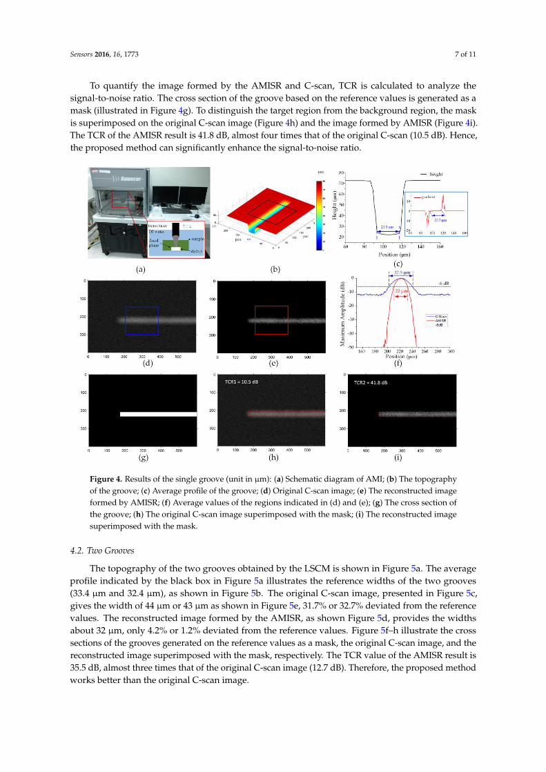
Experimental verification on a complex defect is further performed, as shown in Figure 6.The reference width of the branch is 25.5 µm obtained from the LSCM, as shown in Figure 6a,b.The original C-scan image (Figure 6c) gives the width of 36 µm in Figure 6e, 41.2% deviated from thereference value. The reconstructed image (Figure 6d) gives the width of 27 µm with 5.9% deviation.The TCR value of the image formed by the AMISR is 31.2 dB (Figure 6h), better than that of the originalC-scan image (12.6 dB in Figure 6g). Thus, the proposed method is also effective for complex defects inresolution improvement and signal-to-noise ratio enhancement.

Here we only focus on the C-scan image and the lateral resolution. The axial resolution canbe acquired from the B-scan image, of which the image-forming method is different and alsohas a corresponding PSF. If we obtain the corresponding PSF, the AMISR can also improve theaxial resolution.

Sensors 2016, 16, 1773 9 of 11Sensors 2016, 16, 1773 9 of 11

Figure 6. Results of complex defect (unit in μm): (a) The topography of the defect; (b) Average

profile of the branch; (c) Original C-scan image; (d) The reconstructed image formed by AMISR; (e)

Average profile of the regions indicated in (c) and (d); (f) The cross section of the defect; (g) The

original C-scan image superimposed with the mask; (h) The reconstructed image superimposed

with the mask.

Here we only focus on the C-scan image and the lateral resolution. The axial resolution can be

acquired from the B-scan image, of which the image-forming method is different and also has a

corresponding PSF. If we obtain the corresponding PSF, the AMISR can also improve the axial

resolution.

5. Conclusions

In this paper, a sparse reconstruction method for micro defect detection in AMI is proposed.

The AMI system is modeled as an LTI system, where the output signal is the observed C-scan

image and the input signal is the ideal C-scan image. When the observed C-scan image is available,

the problem of estimating the ideal C-scan image is a deblurring problem, where the key parameter

is the PSF. Here, we develop a finite element model for AMI to simulate the detection of micro

defects and acquire the PSF of the system. By using the PSF as the blur-kernel, we reconstruct the

deblurred image from the oversampled C-scan image based on l1-norm regularization, improving

the resolution and enhancing signal-to-noise ratio. Single groove and two grooves together with a

Figure 6. Results of complex defect (unit in µm): (a) The topography of the defect; (b) Average profileof the branch; (c) Original C-scan image; (d) The reconstructed image formed by AMISR; (e) Averageprofile of the regions indicated in (c) and (d); (f) The cross section of the defect; (g) The original C-scanimage superimposed with the mask; (h) The reconstructed image superimposed with the mask.

5. Conclusions

In this paper, a sparse reconstruction method for micro defect detection in AMI is proposed.The AMI system is modeled as an LTI system, where the output signal is the observed C-scan image andthe input signal is the ideal C-scan image. When the observed C-scan image is available, the problemof estimating the ideal C-scan image is a deblurring problem, where the key parameter is the PSF.Here, we develop a finite element model for AMI to simulate the detection of micro defects andacquire the PSF of the system. By using the PSF as the blur-kernel, we reconstruct the deblurred imagefrom the oversampled C-scan image based on l1-norm regularization, improving the resolution andenhancing signal-to-noise ratio. Single groove and two grooves together with a complex defect areused for verification. The experimental results prove that the method has a significant improvement indetection accuracy and signal-to-noise ratio compared to the original C-scan.

Sensors 2016, 16, 1773 10 of 11

Acknowledgments: The authors are grateful for the financial supports by the National Key Basic Research SpecialFund of China (Grant No. 2015CB057205), the National Natural Science Foundation of China (Grant No. 51305179),the Program for Changjiang Scholars and Innovative Research Team in University (No. IRT13017), and the NaturalScience Foundation of Jiangsu Province (China, No. BK20160183).

Author Contributions: Yichun Zhang and Lei Su conceived and designed the simulations; Yichun Zhang andKepeng Chen performed the AMI experiments; Xiao Wang and Yuan Hong contributed with CLSM; Yichun Zhang,Tielin Shi, and Guanglan Liao analyzed the data; Yichun Zhang and Guanglan Liao wrote the paper.

Conflicts of Interest: The authors declare no conflict of interest.

Abbreviations

The following abbreviations are used in this manuscript:

AMI Acoustic microscopy imagingSAM Scanning acoustic microscopyPSF Point spread functionTCR Target-to-clutter ratioLTI Linear time invariantISTA Iterative shrinkage-thresholding algorithmAMISR Acoustic microscopy imaging sparse reconstructionVT Virtual transducerICP Inductive couple plasmasLSCM Laser scanning confocal microscopy

References

1. Wang, F.L.; Wang, F. Rapidly void detection in TSVs with 2-D X-ray imaging and artificial neural networks.IEEE Trans. Semicond. Manuf. 2014, 2, 246–251. [CrossRef]

2. Wang, F.L.; Wang, F. Void Detection in TSVs with X-ray image multithreshold segmentation and artificialneural networks. IEEE Trans. Compon. Packag. Manuf. 2014, 7, 1245–1250. [CrossRef]

3. Lu, X.N.; Liao, G.L.; Zha, Z.Y.; Xia, Q.; Shi, T.L. A novel approach for flip chip solder joint inspection basedon pulsed phase thermography. NDT E Int. 2011, 6, 484–489.

4. Brand, S.; Czurratis, P.; Hoffrogge, P.; Temple, D.; Malta, D.; Reed, J.; Petzold, M. Extending acousticmicroscopy for comprehensive failure analysis applications. J. Mater. Sci. Mater. Electron. 2011, 10, 1580–1593.[CrossRef]

5. Martin, E.; Larato, C.; Clément, A.; Saint-Paul, M. Detection of delaminations in sub-wavelength thickmulti-layered packages from the local temporal coherence of ultrasonic signals. NDT E Int. 2008, 4, 280–291.

6. Brand, S.; Lapadatu, A.; Djuric, T.; Czurratis, P.; Schischka, J.; Petzold, M. Scanning acoustic gigahertzmicroscopy for metrology applications in three-dimensional integration technologies. J. Micro/Nanolithogr.MEMS MOEMS 2014, 13, 011207. [CrossRef]

7. Errico, C.; Pierre, J.; Pezet, S.; Desailly, Y.; Lenkei, Z.; Couture, O.; Tanter, M. Ultrafast ultrasound localizationmicroscopy for deep super-resolution vascular imaging. Nature 2015, 7579, 499–502. [CrossRef] [PubMed]

8. Viessmann, O.M.; Eckersley, R.J.; Christensen-Jeffries, K.; Tang, M.X.; Dunsby, C. Acoustic super-resolutionwith ultrasound and microbubbles. Phys. Med. Biol. 2016, 18, 6447–6458. [CrossRef] [PubMed]

9. Kwak, D.R.; Yoshida, S.; Sasaki, T.; Todd, J.A.; Park, I.K. Evaluation of near-surface stress distributions indissimilar welded joint by scanning acoustic microscopy. Ultrasonics 2016, 67, 9–17. [CrossRef] [PubMed]

10. Su, L.; Zha, Z.Y.; Lu, X.N.; Shi, T.L.; Liao, G.L. Using BP network for ultrasonic inspection of flip chip solderjoints. Mech. Syst. Signal Process. 2013, 32, 183–190. [CrossRef]

11. Su, L.; Shi, T.L.; Xu, Z.S.; Lu, X.N.; Liao, G.L. Defect inspection of flip chip solder bumps using an ultrasonictransducer. Sensors 2013, 12, 16281–16291. [CrossRef]

12. Zhang, G.M.; Zhang, C.Z.; Harvey, D.M. Sparse signal representation and its applications in ultrasonic NDE.Ultrasonics 2012, 3, 351–363. [CrossRef] [PubMed]

13. Zhang, G.M.; Harvey, D.M.; Braden, D.R. Advanced acoustic microimaging using sparse signalrepresentation for the evaluation of microelectronic packages. IEEE Trans. Adv. Packag. 2006, 29, 271–283.[CrossRef]

14. Mor, E.; Aladjem, M.; Azoulay, A. Cluster-enhanced sparse approximation of overlapping ultrasonic echoes.IEEE Trans. Ultrason. Ferroelectr. Freq. Control 2015, 2, 373–386. [CrossRef] [PubMed]

Sensors 2016, 16, 1773 11 of 11

15. Carcreff, E.; Bourguignon, S.; Idier, J.; Simon, L. A linear model approach for ultrasonic inverse problemswith attenuation and dispersion. IEEE Trans. Ultrason. Ferroelectr. Freq. Control 2014, 7, 1191–1203. [CrossRef][PubMed]

16. Jin, H.R.; Yang, K.J.; Wu, S.W.; Wu, H.T.; Chen, J. Sparse deconvolution method for ultrasound images basedon automatic estimation of reference signals. Ultrasonics 2016, 67, 1–8. [CrossRef] [PubMed]

17. Wu, H.T.; Chen, J.; Wu, S.W.; Jin, H.R.; Yang, K.J. A model-based regularized inverse method for ultrasonicB-scan image reconstruction. Meas. Sci. Technol. 2015, 26, 10540110. [CrossRef]

18. Guarneri, G.; Pipa, D.; Junior, F.; de Arruda, L.; Zibetti, M. A sparse reconstruction algorithm for ultrasonicimages in nondestructive testing. Sensors 2015, 4, 9324–9343. [CrossRef] [PubMed]

19. Canumalla, S. Resolution of broadband transducers in acoustic microscopy of encapsulated ICs: Transducerselection. IEEE Trans. Compon. Packag. Technol. 1999, 4, 582–592. [CrossRef]

20. Lee, C.S.; Zhang, G.M.; Harvey, D.M.; Qi, A. Characterization of micro-crack propagation through analysisof edge effect in acoustic microimaging of microelectronic packages. NDT E Int. 2016, 79, 1–6.

21. Lee, C.S.; Zhang, G.M.; Harvey, D.M.; Ma, H.W.; Braden, D.R. Finite element modelling for the investigationof edge effect in acoustic micro imaging of microelectronic packages. Meas. Sci. Technol. 2016, 27, 25601.[CrossRef]

22. Lee, C.S.; Zhang, G.M.; Harvey, D.M.; Ma, H.W. Development of C-Line plot technique for thecharacterization of edge effects in acoustic imaging: A case study using flip chip package geometry.Microelectron. Reliab. 2015, 12, 2762–2768. [CrossRef]

23. Lee, C.S. Numerical Study for Acoustic Micro-Imaging of Three Dimensional Microelectronic Packages.Ph.D. Thesis, Liverpool John Moores University, Liverpool, UK, 2014.

24. Efrat, N.; Glasner, D.; Apartsin, A.; Nadler, B.; Levin, A. Accurate blur models vs. image priors in singleimage super-resolution. In Proceedings of the IEEE International Conference on Computer Vision (ICCV),New York, NY, USA, 29 August 2013; pp. 2832–2839.

25. Krishnan, D.; Tay, T.; Fergus, R. Blind deconvolution using a normalized sparsity measure. In Proceedings ofthe IEEE Computer Vision and Pattern Recognition (CVPR), Providence, RI, USA, 20 June 2011; pp. 233–240.

26. Beck, A.; Teboulle, M. A fast iterative shrinkage-thresholding algorithm for linear inverse problems. SIAM J.Imaging Sci. 2009, 2, 183–202. [CrossRef]

27. Shao, W.Z.; Li, H.B.; Elad, M. Bi-l0-l2-norm regularization for blind motion deblurring. J. Vis. Commun.Image Represnet. 2015, 33, 42–59. [CrossRef]

28. Tuysuzoglu, A.; Kracht, J.M.; Cleveland, R.O.; Cetin, M.; Karl, W.C. Sparsity driven ultrasound imaging.J. Acoust. Soc. Am. 2012, 21, 1271–1281. [CrossRef] [PubMed]

© 2016 by the authors; licensee MDPI, Basel, Switzerland. This article is an open accessarticle distributed under the terms and conditions of the Creative Commons Attribution(CC-BY) license (http://creativecommons.org/licenses/by/4.0/).