Sparse Independent Vector Analysis: Dictionary Design using a fast

ICA/IVA Mixture Model

2008 SIAM Conference on Imaging ScienceJuly 7, 2008

Jason A. PalmerKen Kreutz-Delgado

Scott Makeig

University of California San DiegoLa Jolla, CA 92093

Outline• Want to do batch Maximum Likelihood

– Large amount of data– Maximum Likelihood asymptotically efficient

• Iterative estimation of the dictionary basis vectors—estimation of sources in overcomplete case is prohibitive– Use Adaptive Newton ICA Mixture Model

• Assumptions:– Only a small number of basis vectors used in each sample– Small number of subsets of bases recur, rather than all possible n choose m combinantions

– Generalized Gaussian Mixture model

• Independent (conditionally sparse and non-sparse) features

• Dependencies– Generalized Gaussian scale mixtures– Variance positive and negative covariance

• Examples– Image bases– EEG bases

Dictionary Design

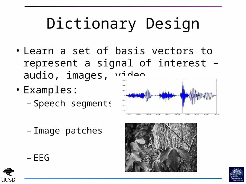
• Learn a set of basis vectors to represent a signal of interest – audio, images, video

• Examples:– Speech segments

– Image patches

– EEG

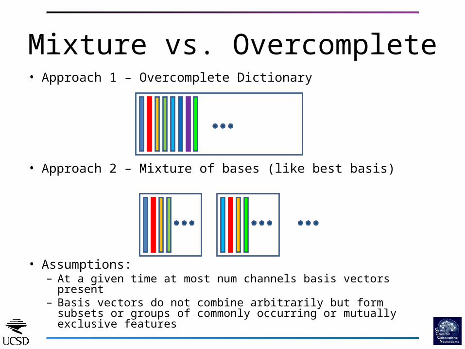
Mixture vs. Overcomplete• Approach 1 – Overcomplete Dictionary

• Approach 2 – Mixture of bases (like best basis)

• Assumptions:– At a given time at most num channels basis vectors present– Basis vectors do not combine arbitrarily but form subsets or

groups of commonly occurring or mutually exclusive features

Maximum Likelihood

• For dictionary design, we assume that a large amount of data is present

• Maximum Likelihood is asymptotically efficient (unbiased and minimum variance)

• Use a “batch” method, iteratively estimate dictionary

• Adapt source densities in an EM context, use a quasi-parametric source model – specifically a mixture model of Generalized Gaussians

ICA Mixture Model• Want to model observations x(t), t = 1,…,N,

different models “active” at different times• Bayesian linear mixture model, h = 1, . . . , M :

• Conditionally linear given the model, :

• Samples are modeled as independent in time:

• Each source density mixture component has unknown location, scale, and shape:

• Generalizes Gaussian mixture model, more peaked, heavier tails

Source Density Mixture Model

Computational Feasibility• We will use an iterative algorithm, in which the basic

steps are:– Estimate the sparse or independent sources or feature

activations given dictionary– Update dictionary based on estimated sources

• For large dimensional problems estimation of sources by iterative or even one-step methods takes non-trivial time, requiring inversion of a matrix for each sample– Example: data = 100 x 1,000,000, time to get sources = 1

ms per sample, one complete iteration takes at least 1000 seconds = 15 minutes, 500 iterations takes 6 days

– Need iterations to be order seconds, so need source estimation to be very fast (less than 1ms) – simple matrix multiplication , can’t afford inversion

Computational Feasibility – Newton

• Even with fast source estimation, we need iteration number to be order 100, not 10,000

• Gradient, and “natural gradient” methods are linearly convergent, very slow at the end

• Newton method yields feasible convergence time

• Using ICA/IVA mixture model allows implementation of Newton method without matrix inversions (2x2 block diagonal Hessian)

• Convergence is really much faster than natural gradient. Works with step size 1!

• Need correct source density model

20 40 60 80 100 120 140 160 180

-2.03

-2.02

-2.01

-2

-1.99

-1.98

-1.97

Convergence Rates

log likelihood

iterationiteration

Independence and Sparsity• Independence means source density factorizes• Sparsity means source density has heavy tails and

high probability of zero• Usually both are assumed• True feature independence may be more useful

than artificially imposed sparsity– Decision theoretic calculations (integrals) simplified

due to density factorization– Coding may be improved by producing true

“innovations” without “interference” in errors• Sparse estimation amounts to enforcing a

particular form (sparse) on the source densities

Marginal Sparsity & Conditional Density

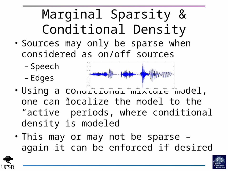
• Sources may only be sparse when considered as on/off sources– Speech– Edges

• Using a conditional mixture model, one can localize the model to the “active” periods, where conditional density is modeled

• This may or may not be sparse – again it can be enforced if desired

Dependence• Not generally possible to decompose

observations into a set of independent features• Types of dependency– Variance dependence (co-occuring features), AB– Mutual exclusion A(not B)

• Gaussian Scale mixtures– Simoncelli, Wainwright – multiscale wavelet

coefficients, steerable pyramid– GSMs are spherically symmetric – not sparse within

subspace• Generalized Gaussian Scale mixtures – maintain

sparsity (directionality) within feature subspace while modeling dependence

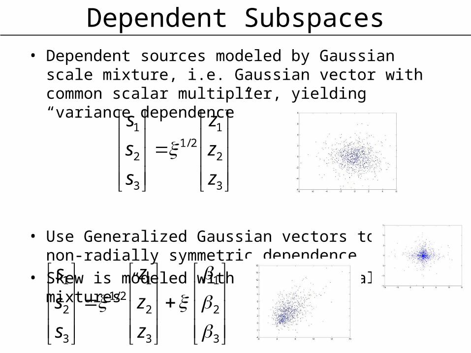
Dependent Subspaces• Dependent sources modeled by Gaussian scale mixture, i.e.

Gaussian vector with common scalar multiplier, yielding “variance dependence”

• Use Generalized Gaussian vectors to model non-radially symmetric dependence

• Skew is modeled with “location-scale mixtures”

3

2

12/1

3

2

1

z

z

z

s

s

s

3

2

1

3

2

12/1

3

2

1

z

z

z

s

s

s

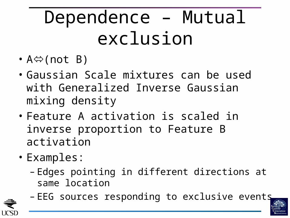
Dependence – Mutual exclusion

• A(not B)• Gaussian Scale mixtures can be used with

Generalized Inverse Gaussian mixing density• Feature A activation is scaled in inverse

proportion to Feature B activation• Examples:– Edges pointing in different directions at same

location– EEG sources responding to exclusive events

Detection of Variance dependence• Variance dependence (subspace structure) can be

determined a priori and enforced, or can be estimated• Estimation strategy – start with assumption of

independence and detect deviations in pairs – then group• Both types of variance dependency can be modeled by

“variance correlation”– Positive variance dependency implies power (variance) in

feature A is high when feature B is high, and A is low when B is low

– Negative variance dependency implies that high power in A implies low power in B (relative to its mean power, or variance)

• If power correlation is large and positive, then features are assigned to variance dependent subspace

• If power correlation is large and negative, then features (or their subspaces) are assigned inverse variance dependence

ICA Mixture Model – Images

• Goal: find an efficient basis for representing image patches. Data vectors are 12 x 12 blocks.

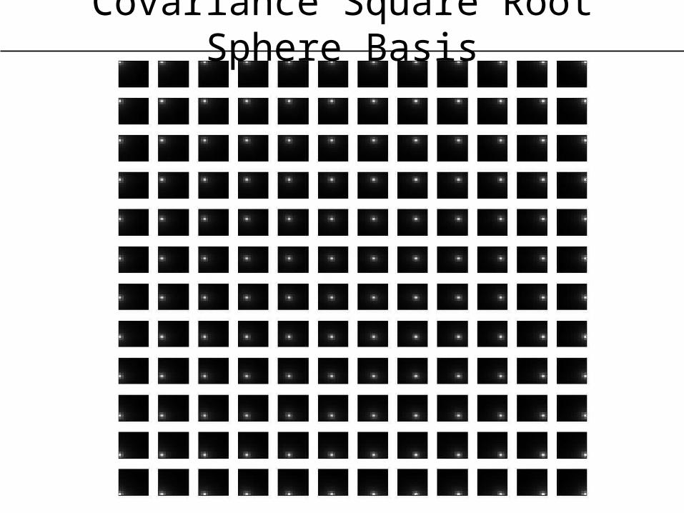
Covariance Square Root Sphere Basis

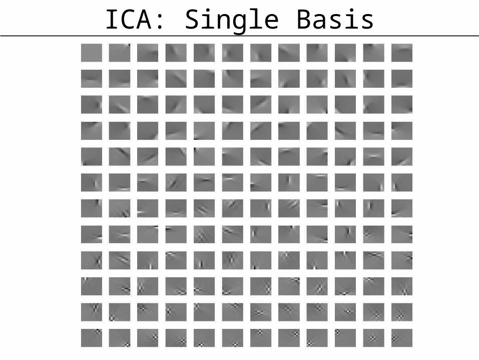
ICA: Single Basis

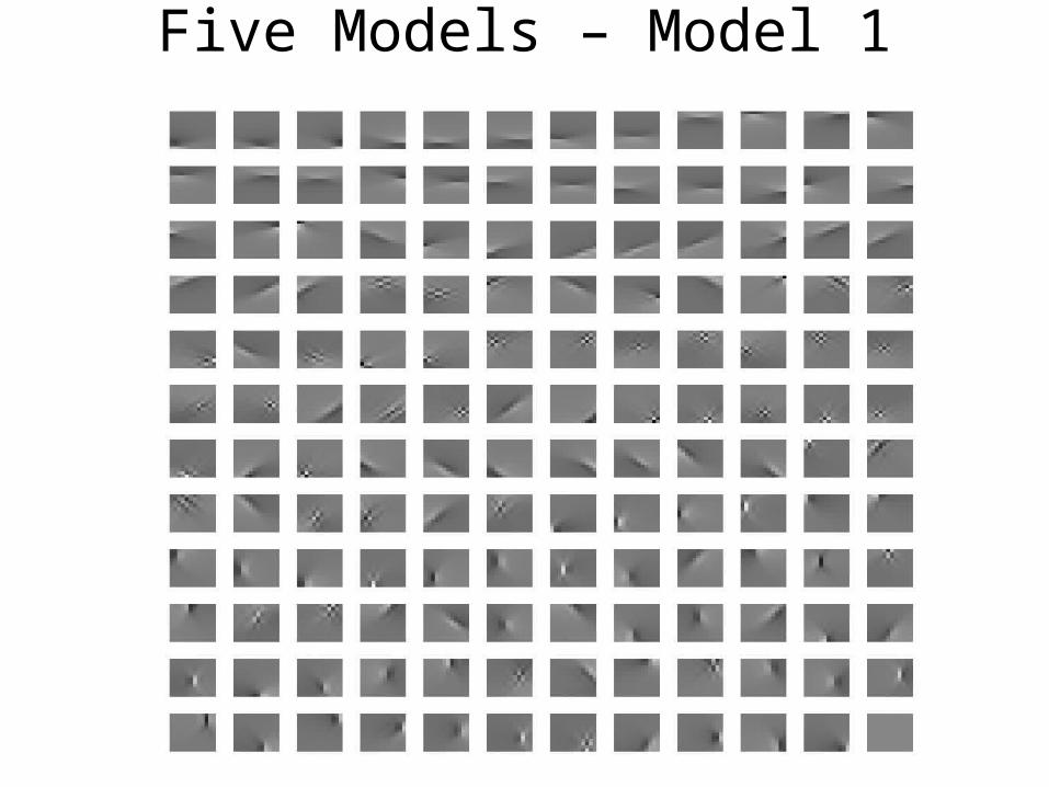
Five Models – Model 1

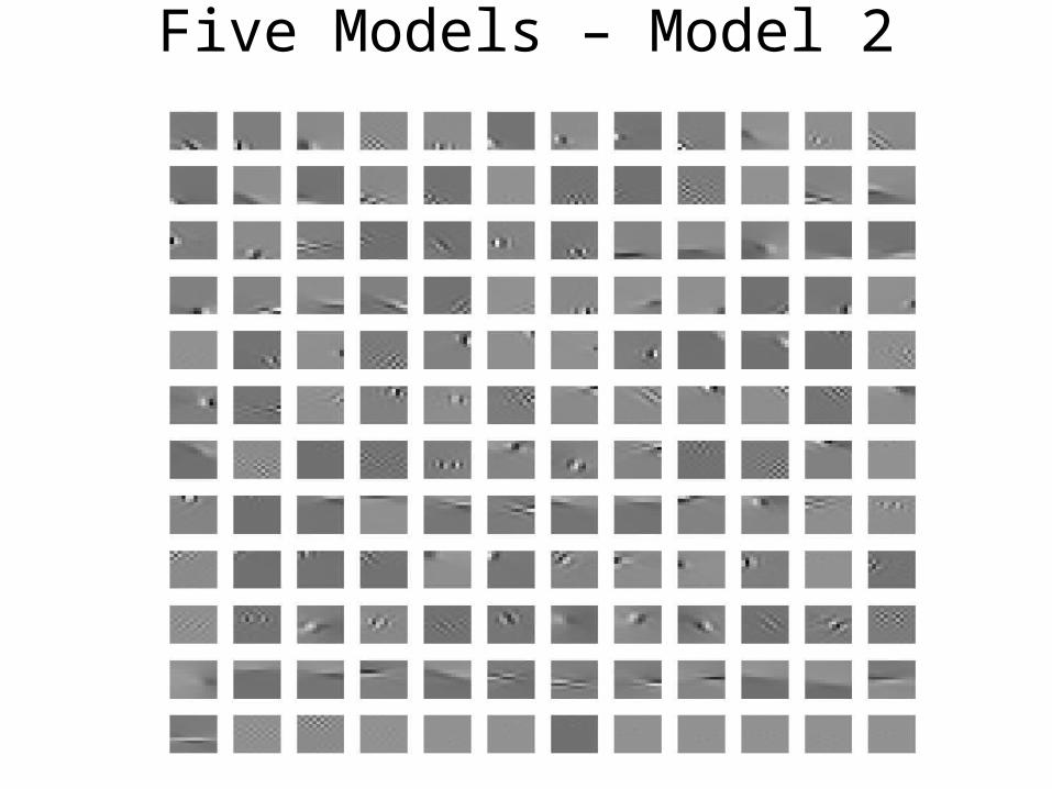
Five Models – Model 2

Five Models – Model 3

Five Models – Model 4

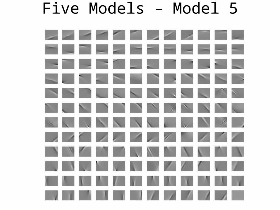
Five Models – Model 5

Variance Dependence

• Variance dependence can be estimated directly using 4th order cross moments

• Find covariance of source power:

• Finds components whose activations are “active” at the same or mutually exclusive times

22 )(,)( tsts jiCov

Variance Correlation – Model 1Before Grouping After Grouping

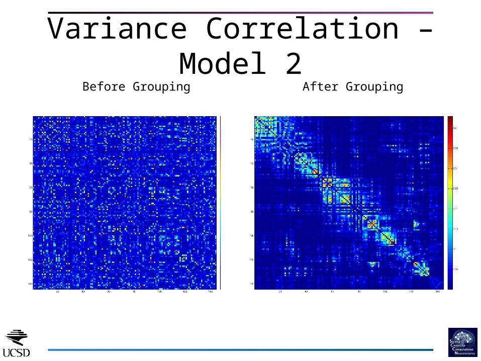
Variance Correlation – Model 2Before Grouping After Grouping

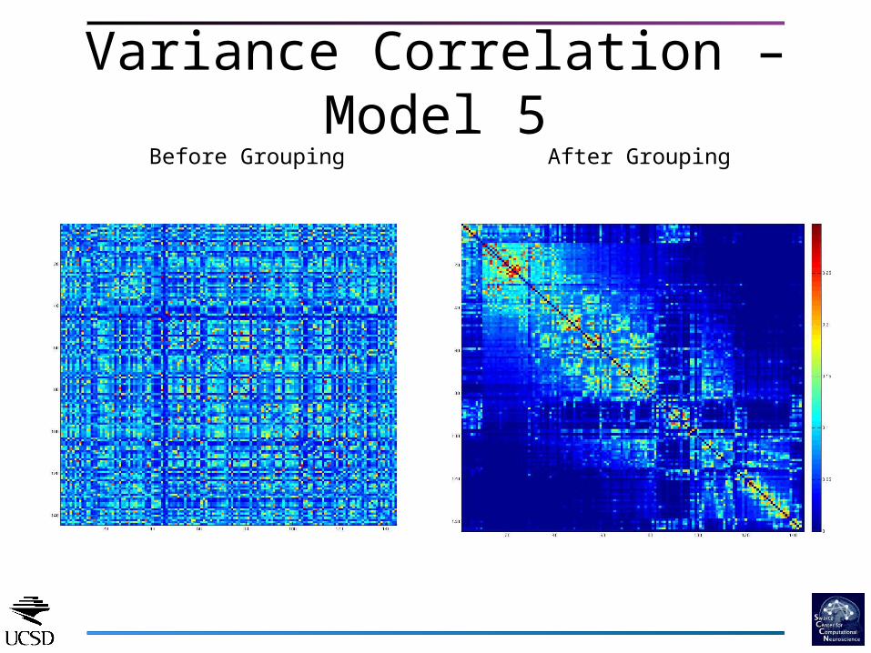
Variance Correlation – Model 5Before Grouping After Grouping

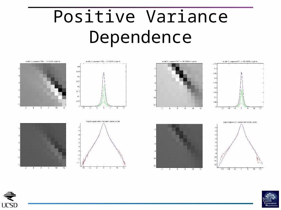
Positive Variance Dependence

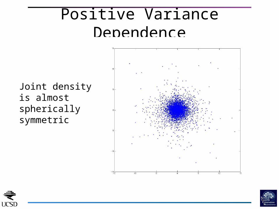
Positive Variance Dependence

Joint density is almost spherically symmetric

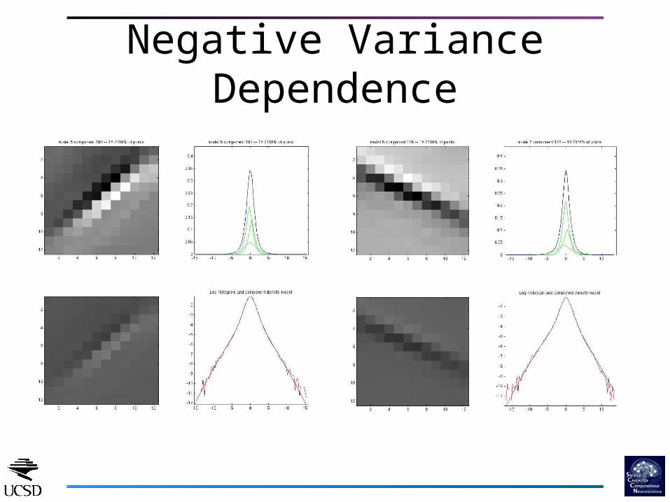
Negative Variance Dependence

Negative Variance Dependence

Joint density has less common activity than product of marginals

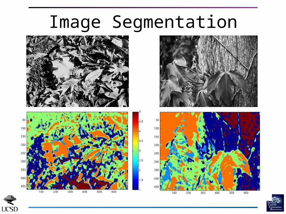
Image Segmentation

Image Segmentation 2

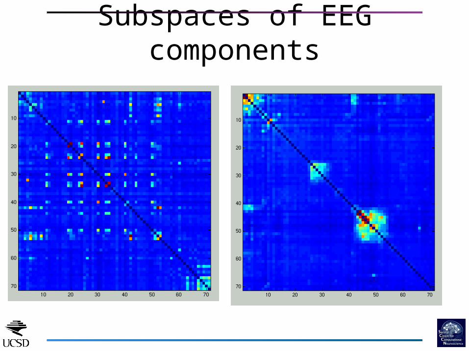
Subspaces of EEG components

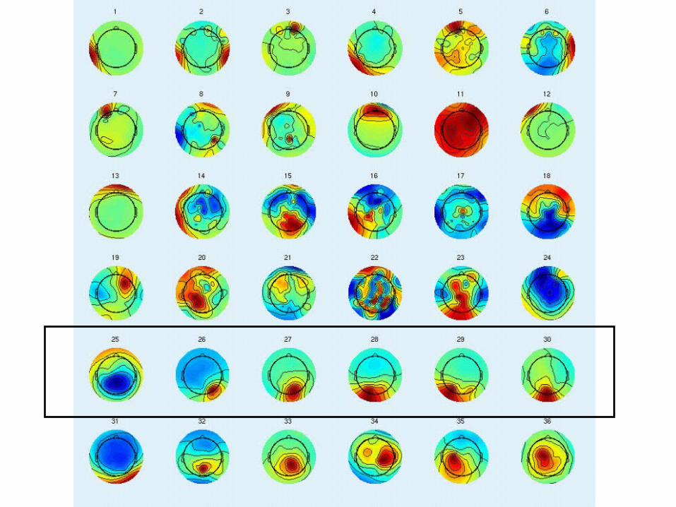
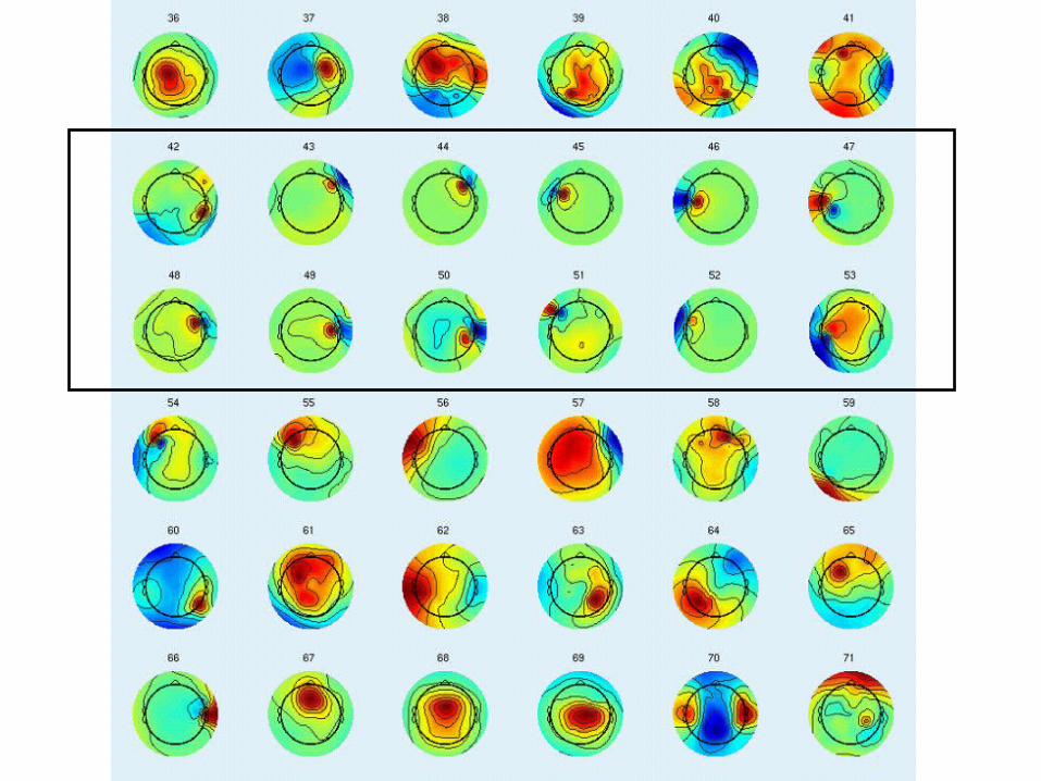
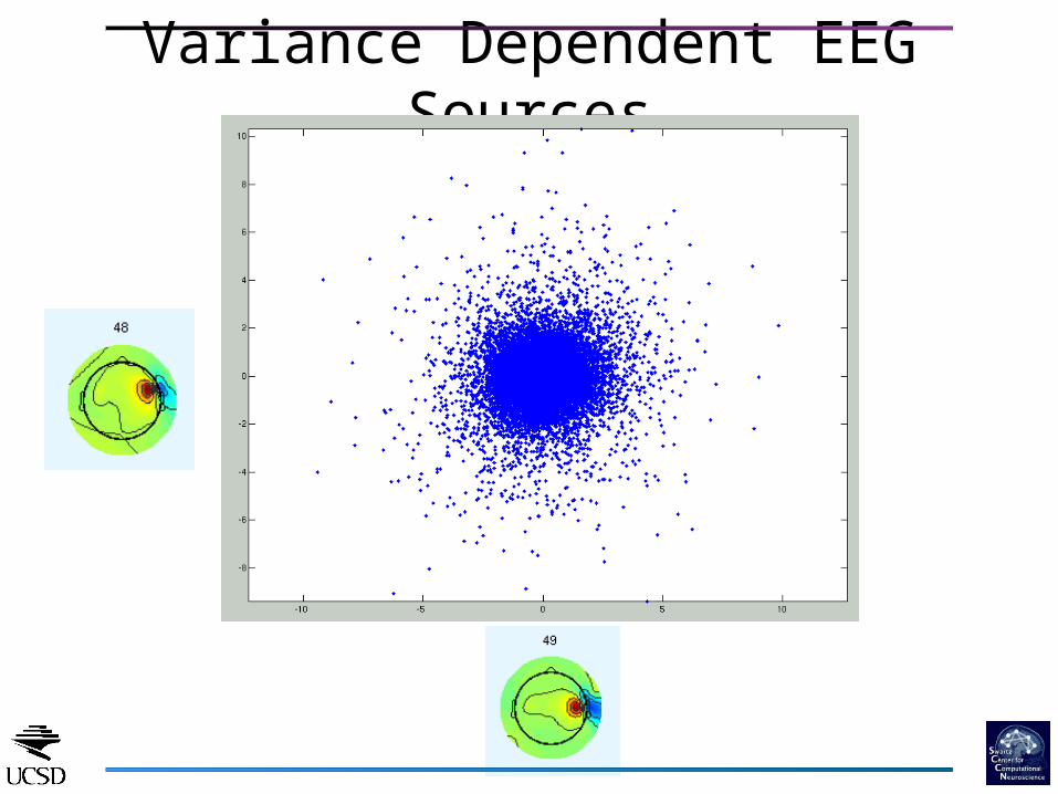
Variance Dependent EEG Sources

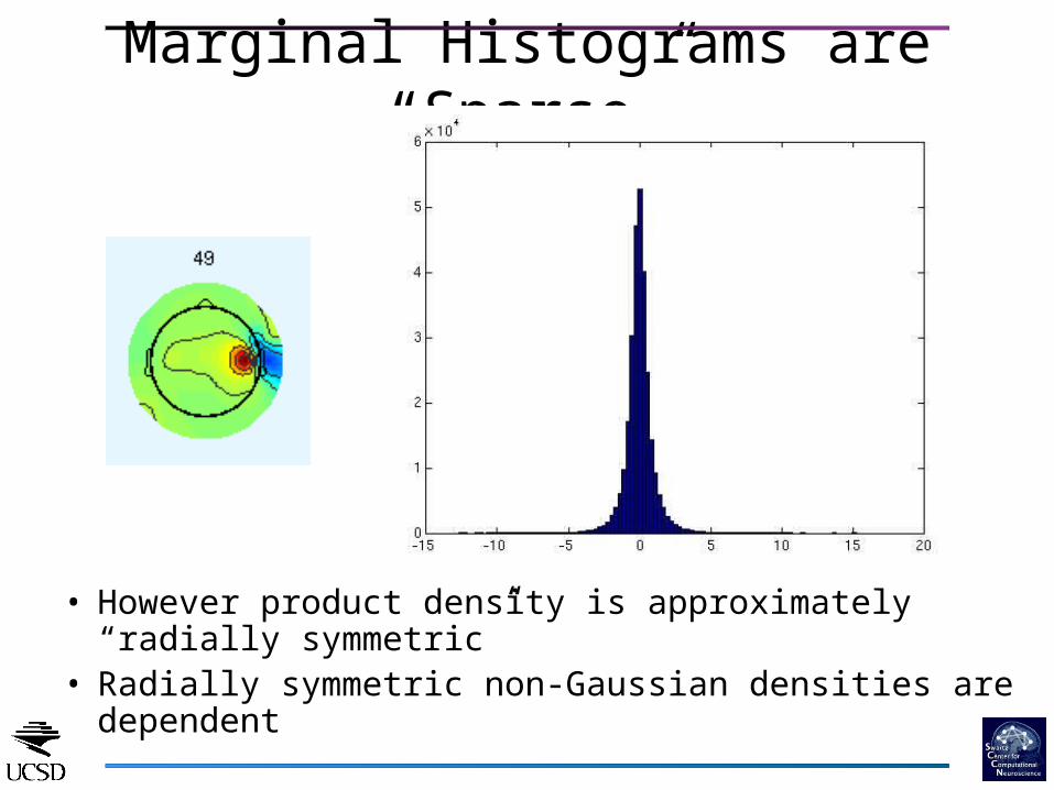
Marginal Histograms are “Sparse”

• However product density is approximately “radially symmetric”

• Radially symmetric non-Gaussian densities are dependent

Conclusion

• We presented an efficient method for learning an overcomplete set of basis

• A Newton algorithm is used with adaptive source densities and a mixture of basis sets

• Dependency is modeled using Generalized Gaussian Scale mixtures

• Variance dependency is detected using variance correlation, which is faster to calculate than mutual information