SPARQL Query Processing with Apache Spark · 2017-05-20 · SPARQL on Spark •Spark: cluster...
47
SPARQL Graph Pattern Processing with Apache Spark GRADES 2017 1 title Hubert Naacke ?P speaker author Olivier Curé Bernd Amann P. et M. Curie Paris 6 University Paris Est Marne-la-Vallée
Transcript of SPARQL Query Processing with Apache Spark · 2017-05-20 · SPARQL on Spark •Spark: cluster...

SPARQL Graph Pattern Processing with Apache Spark
GRADES 2017 1
title
Hubert Naacke
?P
speaker
author
Olivier Curé
Bernd Amann
P. et M. Curie Paris 6
University
Paris Est Marne-la-Vallée

Context
• Big RDF data • Linked Open Data impulse: ever growing RDF content
• Large datasets: billions of <subject, prop, object> triples • e.g. DBPedia
• Query RDF data in SPARQL • The building block is a Basic Graph Pattern (BGP) query
• e.g.:
2
Snowflake pattern from WatDiv benchmark
Chain pattern from LUBM benchmark
GRADES 2017
t2 t3 ?z ?y
t1
advisor teacherOf type Course
includes offers ?x ?u Retail0

Cluster computing platforms
• Cluster computing platforms provide • main memory data management
• distributed and parallel data access and processing
• fault-tolerance, highly availability
➭ Leverage on existing platform • e.g. Apache Spark
GRADES 2017 3

SPARQL on Spark Architecture
GRADES 2017
4
Cluster ressource management
Distributed File system
Resilient Distributed Datastructures (RDD)
SPARQL
SQL
SPARQL
DF
SPARQL
RDD
Hybrid
DF
Hybrid
RDD Our
solutions
SPARQL Graph Pattern query
RDF triples
RDF triples
no compression
DataFrame (DF)
SQL
GraphX data compression

SPARQL query evaluation: Challenges
• Requirements • Low memory usage: no data replication, no indexing
• Fast data preparation: simple hash-based <Subject> partitioning
• Challenges • Efficiently evaluate parallel and distributed join plans with Spark
➭ Favor local computation
➭ Reduce data transfers
• Benefit from several join algorithms • Local partitioned join: no transfer
• Distributed partitioned join
• Broadcast join
GRADES 2017 5

Solution
• Local subquery evaluation • Merge multiple triple selections aka shared scan
• Distributed query evaluation • Cost model for partitioned and broadcast joins
• Generate Hybrid join plans, dynamic programming
GRADES 2017 6

cost(Q92) =
m * (Ct2 + Ct3)
cost(Q93) =
Ct1 + m * Ct3
cost(Q91) =
Ct1 + Ct2 + Ct2 ⨝ t3
with :
Cpattern = transferCost(pattern)
θcomm is the unit tranfer cost
m = #computeNodes - 1
Plan cost:
SELECT * WHERE {
?x advisor ?y .
?y teacherOf ?z .
?z type Course }
Triple patterns of Q9
SPARQL Hybrid
plan
Q93
⋈z
t2 t3
B
y
⋈y
t1
P
x
t2 t3 ?z ?y
t1
advisor teacherOf type
SPARQL RDD
plan
Q91
⋈z
t2 t3
P
y z
⋈y
t1
P
x
Distribute Partitioned join ⋈
P
SPARQL DF
plan
Q92
⋈y
t1 t2
B
x
⋈z
t3
B
Broadcast Broadcast join ⋈
B Legend:
Hybrid plan : example and cost model

Performance comparison with S2RDF
• S2RDF at VLDB 2016 • Same dataset (1B triples) & queries
• Various query patterns: • Star, snowFlake, Complex
GRADES 2017 8
Star Snowfake Complex
➭ One dataset: <Subject> partitioning Hybrid DF accelerates DF up to 2.4 times
➭ One dataset per property: <Property> and <Subject> partitioning Hybrid accelerates S2RDF up to 2.2 times

Take home message
• Existing cluster computing platforms are mature enough to process SPARQL queries at large scale.
• To accelerate query plans: • Provide several distributed join algorithms
• Allows for mixing several join algorithms
More info at the poster session …
Thank you. Questions ?
GRADES 2017 9

Existing solutions
• S2RDF (VLDB 2016) • Spark
• Long data preparation time
• Use a single join algo
• CliqueSquare (ICDE 2015) • Hadoop platform
• Data replicated 3 times: by subject, prop and object
• AdPart (VLDBJ 2016) • Native distributed layer
• "semi-join based" join algorithm
• Distributed RDFox (ISWC 2016) • Native distributed layer
• Data shuffling
GRADES 2017 10
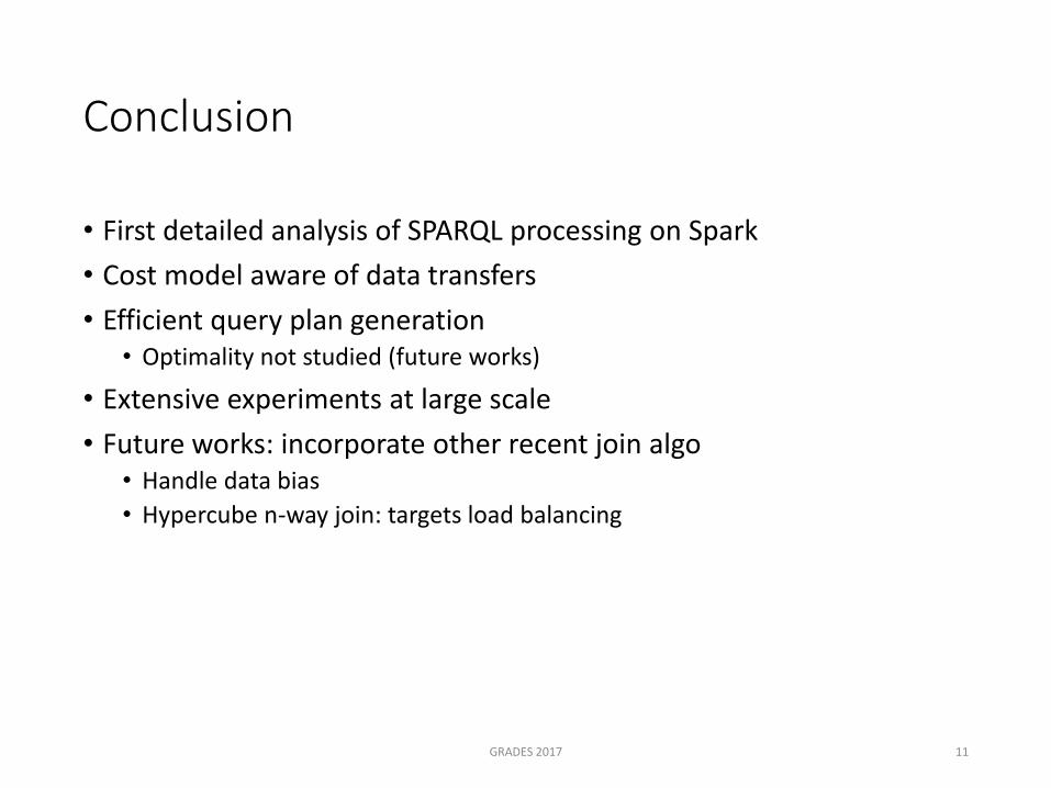
Conclusion
• First detailed analysis of SPARQL processing on Spark
• Cost model aware of data transfers
• Efficient query plan generation • Optimality not studied (future works)
• Extensive experiments at large scale
• Future works: incorporate other recent join algo • Handle data bias
• Hypercube n-way join: targets load balancing
GRADES 2017 11

Thank you
Questions ?
GRADES 2017 12

Extra slides
•
GRADES 2017 13

SPARQL RDD
plan
Q91
⋈z
t2 t3
P
y z
⋈y
t1
P
x
SPARQL SQL
plan
Q92
⋈y
t1 t2
B
x
⋈z
t3
B
SPARQL Hybrid
plan
Q93
⋈z
t2 t3
B
y
⋈y
t1
P
x
with :
Cpattern = θcomm * size(pattern)
θcomm is the unit tranfer cost
m = #computeNodes - 1
cost(Q92) =
m * (Ct2 + Ct3)
cost(Q93) =
Ct1 + m * Ct3
Plan cost:
cost(Q91) =
Ct1 + Ct2 + Ct2 ⨝ t3
Hybrid plan: Cost model

s3 p1 o2 s2 p1 o2 s2 p3 o4
Data distribution (1/2) Hash-based partitioning
Dataset (subject, prop, object)
BDA 2016 15
s1 p1 o1 s1 p2 o3
s1 p1 o1 s2 p1 o2 s3 p1 o2 s1 p2 o3 s2 p3 o4 ...
Part 1 Part 2 Part N
Partitioning is • Straightforward
• Simple map-reduce task
• No preparation overhead requirement
• Hash-based partitioning on subject

Data distribution (2/2) over a cluster
BDA 2016 16
Piece of data
Operation
Result
Compute node 1 node 2 node N
Memory
CPU
Memory
Comm is expensive
Ressources:

Parallel and distributed data processing workflow (1/2)
BDA 2016 17
Part 1
Part 2
Part N
Local (MAP) Operation
Partitioned dataset
select
Result1
select
Result2
select
ResultN
Examples of local MAP operations: selection, projection, join on subject
Partitioned Result
Compute node 1 node 2 node N

BDA 2016 18
Part 2
Part n Dataset
Global Operation
Part 1
Result1
Data transfers
Global (REDUCE) Operation
Global Operation
Global Operation
Result2
Resultn
Examples of global REDUCE operations : join, sort, distinct
Parallel and distributed data processing workflow (2/2)

Join processing wrt. query pattern
Data:
BDA 2016 19
lab at ?L ?P ?V
Star query: • Find laboratory and name of persons
P2 lab L3 P2 age 20 P2 name Bob P4 lab L1
P1 lab L1 P1 name Ali P3 lab L2 P3 name Clo
L1 at Poitiers L1 since 2000 L3 at Paris L3 staff 200
L2 at Aix L2 at Toulon L2 partner L1 …
Transfer lab or at
lab
name ?P
?L
?N
?L age
Snowflake query:
No transfer
Chain query: • Find lab and its city for persons
lab ?L ?P
?a
age
name ?n
at ?V
staff ?s
?N partner Complex query

Join algorithms
• Partitioned join (Pjoin) • Distribute data
• Broadcast join (Brjoin) • Broadcast to all
• Hybrid join (contribution) • Distribute and/or broadcast
• Based on a cost model
BDA 2016 20
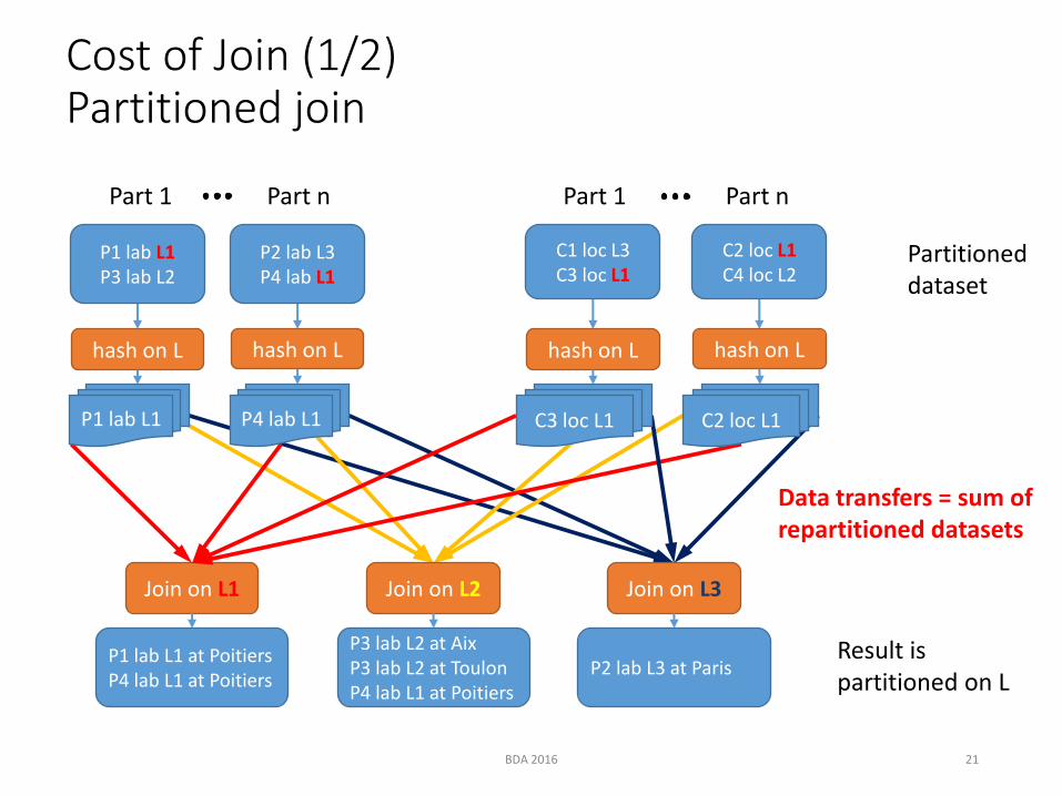
Join on L1
Result is partitioned on L
Join on L2
P1 lab L1 at Poitiers P4 lab L1 at Poitiers
P3 lab L2 at Aix P3 lab L2 at Toulon P4 lab L1 at Poitiers
Join on L3
P2 lab L3 at Paris
Data transfers = sum of repartitioned datasets
Cost of Join (1/2) Partitioned join
BDA 2016 21
hash on L hash on L hash on L hash on L
Partitioned dataset
P1 lab L1 P3 lab L2
C1 loc L3 C3 loc L1
P2 lab L3 P4 lab L1
C2 loc L1 C4 loc L2
Part 1 Part n Part 1 Part n
P1 lab L1 P4 lab L1 C3 loc L1 C2 loc L1

Cost of join(2/2) Broadcast Join
BDA 2016 22
Join on L
Result preserves the target partitioning
P1 lab L1 P3 lab L2
P2 lab L3 P4 lab L1
Join on L
P1 lab L1 at Poitiers P3 lab L2 at Aix P3 lab L2 at Toulon
Part 1 Part n Part 1 Part n
P2 lab L3 at Paris P4 lab L1 at Poitiers
L1 at Poitiers L2 at Aix
L2 at Toulon L3 at Paris
Larger target dataset Smaller broadcast dataset
Data transfers = Small dataset * nb of compute nodes
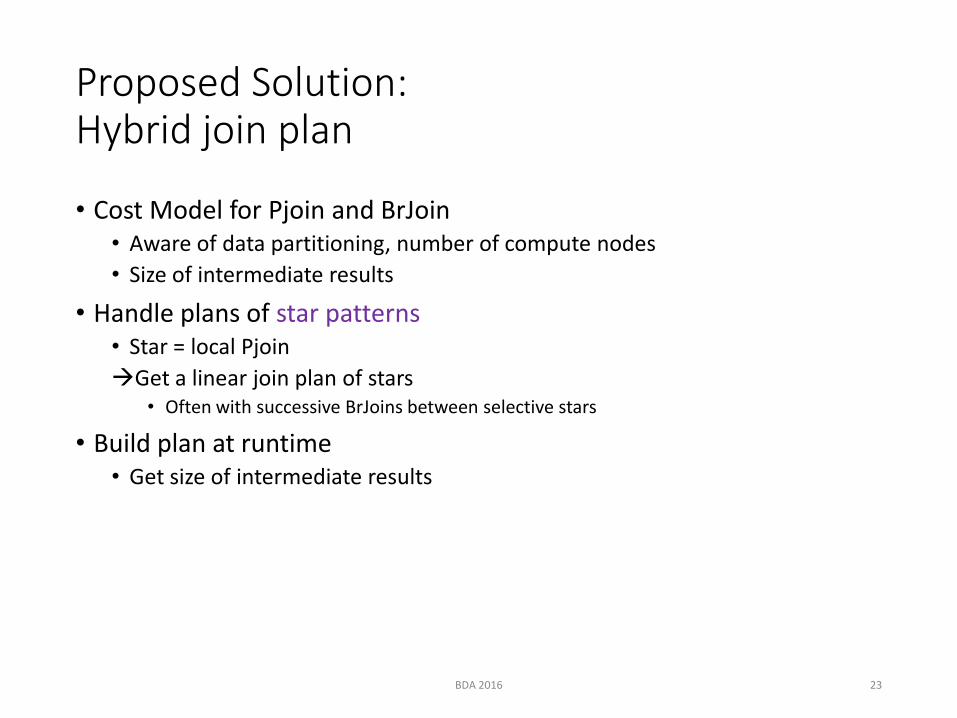
Proposed Solution: Hybrid join plan
• Cost Model for Pjoin and BrJoin • Aware of data partitioning, number of compute nodes
• Size of intermediate results
• Handle plans of star patterns • Star = local Pjoin
Get a linear join plan of stars
• Often with successive BrJoins between selective stars
• Build plan at runtime • Get size of intermediate results
BDA 2016 23

Build Hybrid join plan
1) Compute all stars: S1, S2,… • Si = Pjoin(t1, t2, …)
2) Join 2 stars, say Si with Sj
• Ensure cost(Si ⨝ Sj) is minimal get Si, Sj and a join algorithm
• Let Temp = Si ⨝ Sj
3) Continue with a 3rd star, say Sk
• Ensure cost(Temp ⨝ Sk) is minimal
and so on …
BDA 2016 24

SPARQL on Spark: Qualitative comparison
Method co-partitioning Join plan Merged selection Query Optimizer
Data Compression
SPARQL RDD
Pjoin
SPARQL DF v 1.5 Pjoin,BrJoin1 poor
SPARQL SQL v 1.5 Pjoin,BrJoin1 cross prod
Hybrid RDD Pjoin,BrJoin+
cost based
Hybrid DF Pjoin,BrJoin+
cost based
BDA 2016 25
Our solutions
supported not supported
Spark interface

Experimental validation: setup
• Datasets
• Cluster • 17 compute nodes
• Resource per node: 12 cores x 2 hyperthreads, 64 GB memory
• 1Gb/s interconnect
• Spark • 16 worker nodes
• Aggregated resources: 300 cores, 800 GB memory
• Solution • Implem written in scala, see companion website
BDA 2016 26
Dataset Name Nb of triples Description
DrugBank 500K Real dataset
LUBM 1.3B Synthetic data, LeHigh Univ
WatDiv 1.1B Synthetic data, Waterloo Univ

Experiments: Performance gain
• Response time for Snowflake Q8 query from LUBM
• 2 dataset sizes: medium (100M triples), large (1B triples)
BDA 2016 27
Dataset size
Achieve higher gain for larger datasets No compression: 4,7 times faster Compressed data 3 times faster
Thanks for your attention
Questions ?
BDA 2016 28

Extra slides
BDA 2016 29
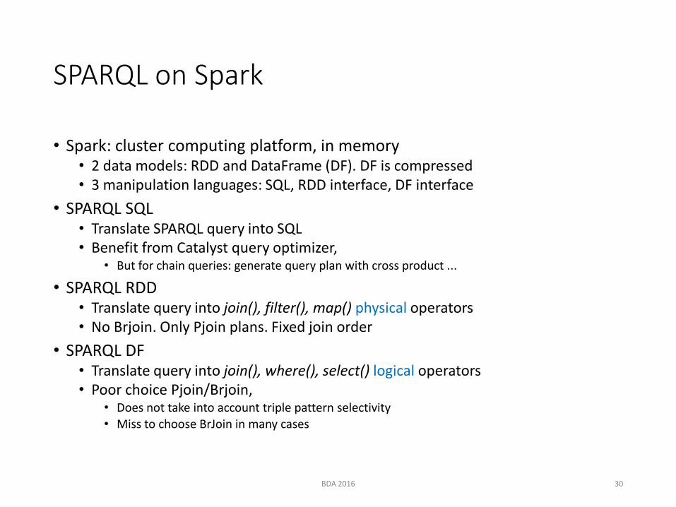
SPARQL on Spark
• Spark: cluster computing platform, in memory • 2 data models: RDD and DataFrame (DF). DF is compressed • 3 manipulation languages: SQL, RDD interface, DF interface
• SPARQL SQL • Translate SPARQL query into SQL • Benefit from Catalyst query optimizer,
• But for chain queries: generate query plan with cross product ...
• SPARQL RDD • Translate query into join(), filter(), map() physical operators • No Brjoin. Only Pjoin plans. Fixed join order
• SPARQL DF • Translate query into join(), where(), select() logical operators • Poor choice Pjoin/Brjoin,
• Does not take into account triple pattern selectivity • Miss to choose BrJoin in many cases
BDA 2016 30

SPARQL on Spark: Hybrid solution
• Combine mutiple triple selections • Prune data to reduce access cost
• Build cost-based optimized plan
• Supports both data models: RDD and DF • Implements missing BrJoin for RDD
• Allows for broadcasting intermediate results
BDA 2016 31

Perf of Star queries
BDA 2016 32

Perf of chain queries
BDA 2016 33

Partitioned join : Detailed algorithm
1) Partition data on the join key Check current data partitioning
2) Distribute (i.e., shuffle) the partitions
3) Compute the join for each key
Data transfers • see formula in the paper (cost of n-ary Pjoin)
BDA 2016 34

Broadcast Join: Detailed algorithm
• Join a smaller dataset with a larger one • Larger dataset = target dataset
1) Broadcat the small dataset to every compute node
2) Compute the join for each partition of the target
Data transfers • see formula in the paper (cost of n-ary Brjoin)
BDA 2016 35

OLD
• OLD
BDA 2016 36

BDA 2016 37
lab at Requête: ?L ?P ?V

Join processing (1)
BDA 2016 38
Part 1
Part n Triple dataset
Join for h(x)=1
Result1
Triple join : x memberOf y . x email z
Result
Select t2 and hash
on x
Resultn
Select t2 and hash
on x
Part 1
Part n
Select t2 and hash
on x
Select t2 and hash
on x

ENLEVER Assumptions and requirements
• Data Volume • Requires a distributed environnement
• Data Velocity • Requires reduced data loading time
• Main memory data management • No data replication
BDA 2016 39

SPARQL Query Processing with Apache Spark
BDA 2016 40
title
?L
?P
speaker
author
Auteur Laboratoire Université
Hubert Naacke LIP6 P. et M. Curie Paris 6
Olivier Curé LIGM Paris Est Marne-la-Vallée
Bernd Amann LIP6 P. et M. Curie Paris 6

Processing a global operation on distributed data
BDA 2016 41
Part 1
Part 2
Part N
Triple dataset
Global Operation
Result
Data transfers
Global operation is not parallel enough, Scalability ?

Join processing wrt. query shape
Data:
BDA 2016 42
lab at ?L ?P ?V
Query: • Find laboratory and city of persons
P2 lab L3 P2 name Bob P4 lab L1
P1 lab L1 P1 name Ali P3 lab L2 P3 name Clo
L1 at Poitiers L1 since 2000 L3 at Paris L3 staff 200
L2 at Aix L2 at Toulon L2 partner L1
Chain:
lab
name ?P
?L Star:
?N
?L
age
lab at ?L ?P ?V Chain:

Data:
lab at ?L ?P ?V
Star query:
P2 lab L3 P2 age 20 P2 name Bob P4 lab L1
P1 lab L1 P1 name Ali P3 lab L2 P3 name Clo
L1 at Poitiers L1 since 2000 L3 at Paris L3 staff 200
L2 at Aix L2 at Toulon L2 partner L1 …
lab
name ?P
?L
?N
?L age
Snowflake query:
Chain query:
lab ?L ?P
?a
age
name ?n
at ?V
staff ?s
?N partner
Complex query

BDA 2016 44

BDA 2016 45

GRADES 2017 46
SELECT * WHERE {
<retailer0> offers ?u .
?u price ?v .
?u validThrough ?w .
?u includes ?x .
?x title ?y .
?x type ?z }
WatDiv F5 includes offers ?x ?u

cc
BDA 2016 47