Spaces with Lusternik–Schnirelmann category n and cone length n+1

qThis work was supported by DFG grant Sche 328/2-1E-mail address: [email protected] (D. Stanley)

Topology 39 (2000) 985}1019

Spaces with Lusternik}Schnirelmann category n andcone length n#1q

Donald Stanley

Department of Mathematical Sciences, University of Alberta, 632 Central Academic Building, Edmonton, Alberta,Canada T6G 2G1

Received 16 July 1998; accepted 26 October 1998

This paper is dedicated to my father

Abstract

We construct a series of spaces, X(n), for each n'0, such that cat(X(n))"n and cl(X(n))"n#1. We showthat the Hopf invariants determine whether the category of a space goes up when attaching a cell of topdimension. We give a new proof of counterexamples to a conjecture of Ganea. Also we introduce sometechniques for manipulating cone decompositions. ( 2000 Published by Elsevier Science Ltd. All rightsreserved.

MSC: primary 55M30; 55P50

Keywords: Lusternik}Schnirelmann category; Cone length; Hopf invariants

1. Introduction

Let X be a space. The Lusternik}Schnirelmann category, LS category, denoted cat(X), wasintroduced in the 1920s as an invariant which gave a lower bound for the number of critical pointsof a function on a closed manifold [20]. The original de"nition was essentially the minimum size ofa covering of the manifold by open sets which are contractible in the manifold. A de"nitionequivalent for CW-complexes was given by Whitehead in terms of the minimum fat wedge(De"nition 2.6) through which the iterated diagonal factors. The de"nition which we will use

0040-9383/00/$ - see front matter ( 2000 Published by Elsevier Science Ltd. All rights reserved.PII: S 0 0 4 0 - 9 3 8 3 ( 9 9 ) 0 0 0 4 7 - 6

(De"nition 2.5) is due to Ganea [14] and is again equivalent to the other two (except for therenormalization of subtracting one) for CW-complexes.

The strong category, denoted Cat(X), was introduced by Fox [11]. In this same paper he gave anexample to show that the notion was not homotopy invariant. This problem is overcome by takingthe minimum over all spaces of the same homotopy type. He also showed that cat(X))Cat(X).The cone length (De"nition 2.7), denoted cl(X), was introduced by Ganea [14] where he proved atthe same time that cone length and strong category are equal. A few years later Takens [27] andindependently Ganea showed that cone length and LS category di!ered by at most one. Howeverthe only examples where the two invariants were known to di!er were coH spaces that are notsuspensions, that is cat(X)"1, cl(X)"2. (The "rst example actually appeared in [4].) Almost 30years later Dupont [7] constructed an example of a space of category three and cone length four.

The reason that the case of cl(X)"1 is easier is that we have the characterization, cl(X)"1 ifand only if X"R>. To see that X is not of some higher cone length we have to somehow look atall possible cone decompositions of it. To solve this problem we develop techniques for handlinggeneral cone decompositions. We introduce the notion of an r-cone receiver (Section 5). Weconstruct an r-cone receiver for our particular space of interest X (Section 6). We then take anyr-cone decomposition of X and map it into its r-cone receiver. This allows us to derive from anyr-cone decomposition one of a very speci"c form (Section 7). We then "nd an obstruction to suchan r-cone decomposition (Section 8). The methods of this section are in the spirit of single loopspace decomposition theory. The obstruction is essentially the attaching map of a cell in a loopspace. For X to have an r-cone decomposition this map must be trivial since the correspondinghomology class needs to be in the image of the Hurewicz homomorphism. To show cat(X)"r weuse a variant of a technique of Iwase [18]. The proof depends on homotopy classes which havenon-trivial Hopf invariants which become trivial after n suspensions. Taken together we reach ourmain goal.

Theorem 1.1. Theorem 9.3 For every r'0 there exists a space X such that cat(X)"r andcl(X)"r#1.

There are a number of other interesting results in the paper. We show that the Hopf invariant(De"nition 3.4) of Berstein and Hilton [4] characterizes when attaching cells of top dimensioncauses the LS category to go up (Theorem 3.6). This fact was known to them in case dimen-sion(X))(cat(X)#1)connectivity(X)!2. Now, however, Hopf invariants can be used to deter-mine the category of any "nite complex. We o!er some cone decompositions of spaces of the formQ]Sn (Theorem 4.1). This gives an alternative (to [18]) proof of counterexamples to a conjecture ofGanea. Also, we give some general lemmas for constructing r-cone receivers out of other ones(Lemmas 5.6, 5.7, 5.12 and 5.13). These may prove useful in the study of cone length of other spaces.

2. Notation and background

In this section we introduce some notation and de"nitions that will be used throughout thepaper. A few facts about CW-complexes are also presented. We make no claim to the originality ofany of the results in this section.

986 D. Stanley / Topology 39 (2000) 985}1019

For the rest of the paper we assume, unless otherwise stated, that all our spaces are simplyconnected, pointed and have the pointed homotopy type of a CW-complex. Also our CW-complexes will have a unique 0-cell and no 1-cells. For any space we will let * denote the basepoint.

Such spaces and maps between them form a category. In general whenever we refer to a map wewill assume unless we state otherwise that it is a map in this category. For this section let X bea space. We let Xn denote the nth Cartesian product of X with itself. When we say that X isa CW-complex we mean that X is a space with a particular CW-structure. If we are workingp-locally Sn and en both denote the p-local versions. We also let * denote the binary operation of thejoin. It is a fact that for spaces of our kind X,>,X*>KRX'>.

We let con(X) denote the connectivity of X. For a map f :XP>, con( f ) denotes the connectivityof f. So con( f )*n if and only if n

H( f ) is an isomorphism for *(n and a surjection for *"n. We

also refer to such a map as an n-equivalence. Throughout the paper we make use of the Serre exactsequence. For a statement and proof of it we refer the reader to Whitehead [29]. Let dim(X) denotethe dimension of X. By this we mean the minimum dimension of a CW-complex equivalent to X. IfX is simply connected and "nite type this means the dimension of the top non-zero cohomologyclass of X. If X is a CW-complex we let X

ndenote the n-skeleton of X, that is the subcomplex with

all cells of dimension less than or equal to n. For a map f : SrPX we let f a : Sr~1PXX denote theadjoint. If X is a CW-complex then there is a cellular chain complex C

H(X) with a canonical basis

induced by the cell structure.Let f :XP> be a map. Let C( f ) denote the reduced cone on f. Explicitly,

C( f )"(>XX]I)/((x, 1)"f (x), (x, 0)"(*, t)"*).

C( f ) is also referred to as the homotopy co"bre of f. There is a canonical map (inclusion)>PC( f ).

A sequence X fP > g

P Z is called a co"bration sequence if ZKC( f ) in a way compatible with

g and the canonical inclusion. In other words such that the obvious diagram commutes up tohomotopy. If we have a commutative diagram

(*)

then we get a canonical map C( f )PC( f @) in the obvious way. Dually, let Fib( f ) denote the pathspace on f. Explicitly,

Fib( f )"M(/,x)3>I]XD/(1)"f (x),/(0)"*N.

Fib( f ) is also referred to as the homotopy "bre of f. There is a canonical map (evaluation)

Fib( f )PX. A sequence Z gP X f

P > is called a "bration sequence if ZKFib( f ) in a waycompatible with g and the canonical evaluation. Again this means we require the obvious diagramto commute up to homotopy. If we have a commutative diagram (*) as above then we geta canonical map Fib( f )PFib( f @) in the obvious way.

It is obvious that taking the homotopy co"bre keeps us in the category of spaces having thepointed homotopy type of CW-complexes. It follows from [22] that taking homotopy "bres does

D. Stanley / Topology 39 (2000) 985}1019 987

as well. In fact, it follows directly if f is a co"bration and in general from the fact that the category ofspaces having the pointed homotopy type of CW-complexes is closed under retracts.

The following lemma was proved by Baues [3].

Lemma 2.1. For i"1, 2 let f (i) : A(i)PB(i) be maps between coxbrantly generated spaces. Then thereis a coxbration sequence

A(1) * A(2)PC( f (1))]B(2)XB(1)CB(2)

B(1)]C( f (2))PC( f (1))]C( f (2)),

where ] denotes the weak product. This sequence is natural in both variables. In other words if fori"1, 2 we have commuting diagrams

then we get a commuting diagram

Proof. See Refs. [3,26]. h

The last lemma implies that if X and > are CW-complexes then X]> is also canonicallya CW-complex (once we have "xed a homeomorphism Sn`r`1+Sn* Sr). It is clear that Xs> isalso canonically a CW-complex. Also for every cellular map f : SnPX, C( f ) is canonicallya CW-complex. Any skeleton of a CW-complex is canonically a CW-complex. We will call all suchCW-structures the canonical ones. For Sn we call its minimal cell structure the canonical one. Thatis the cell structure with one 0-cell and one n-cell. All this implies that we have a canonical cellstructure on (Sn)r and therefore on ¹r(Sn).

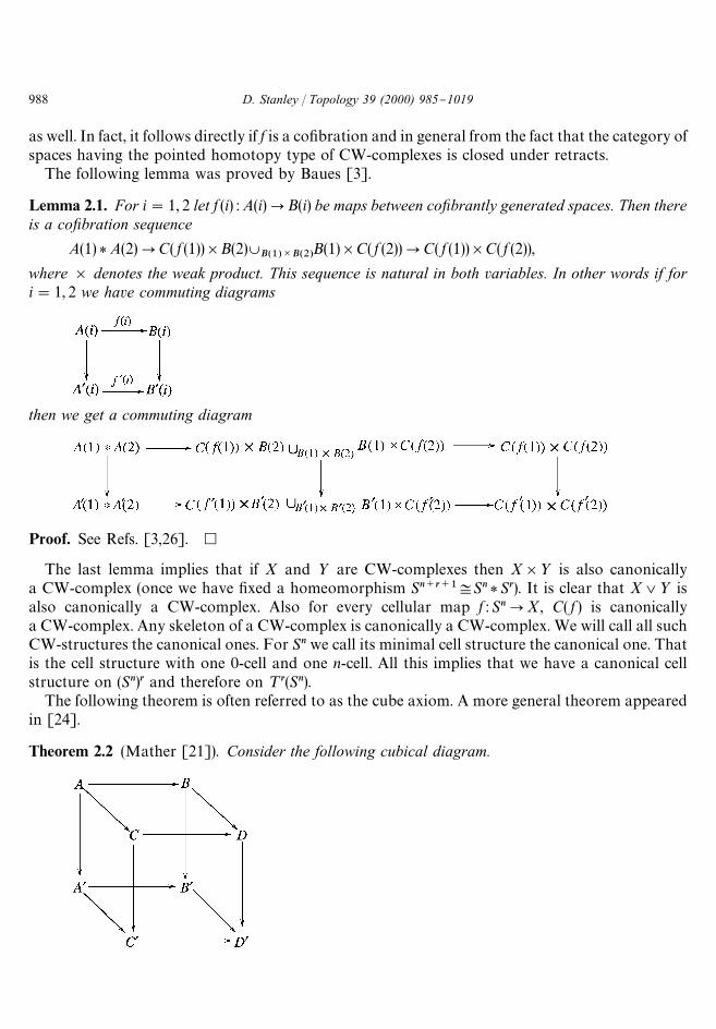
The following theorem is often referred to as the cube axiom. A more general theorem appearedin [24].

Theorem 2.2 (Mather [21]). Consider the following cubical diagram.


Assume that the bottom face is a homotopy pushout and that all sides are homotopy pullbacks. Then thetop face is a homotopy pushout.

De5nition 2.3. Let X be a space. We de"ne "bration sequences.

Fn(X) inP G

n(X) pnP X.

Let G0(X)"* and p

0the inclusion. Let F

n"Fib(p

n) and G

n`1(X)"C(i

n). We get the extension

pn`1

by mapping Fn]I using the paths /.

Let *1X"X*X and *nX"*n~1X* X.

Theorem 2.4. Fn(X)K*nXX.

Proof. See Ref. [13, Theorem 1.1]. h

Observe that for example G1(X)KRXX. Another way of thinking of G

n(X) is as the nth stage of

Milnor's classifying space construction for XX. We have not described it in this way since we wantto make use of the fact that G

n(X) is a case of Ganea's "bre}co"bre construction. Our de"nition

di!ers from Ganea's original one [14] in that we do not turn our pn's into "brations. This

procedure is implicit in taking homotopy "bres. Because of this di!erence our next de"nition alsodi!ers from Ganea's in that we only require homotopy sections. Throughout the paper we willoften refer to homotopy sections as sections.

De5nition 2.5. We say a space X has category less than or equal to n, cat(X))n, if and only ifpnhas a homotopy section.

De5nition 2.6. Let

¹n(X)"M(x1,2, x

n)3Xn D x

i"* for some iN.

¹n(X) is called the fat wedge.

An alternative de"nition of category, due to Whitehead, uses the fat wedge. In his de"nitionX has category less than or equal to n if and only if the iterated diagonal XPXn`1 factors through¹n`1(X) up to homotopy. The two de"nitions concur on a subcategory of the category oftopological spaces containing the category of spaces having the homotopy type of a CW-complex[15].

Let X be a space. Let X(i), =(i) be sequences of spaces such that X(0)"*, X(n)"X and suchthat there exist co"bration sequences

=(i)PX(i)PX(i#1).

We then call MX(i)N an n-cone decomposition of X.


De5nition 2.7. Let cl(X) denote the cone length of X. That is the minimal n such that X has ann-cone decomposition.

Theorem 2.8. cat(X))cl(X))cat(X)#1.

Proof. The "rst inequality follows directly from [29, Chapter X, Theorem 1.6] or [4, Theorem 2.6].The second inequality follows from the main theorem of [27] (see also Section 5) and [14,Proposition 2.1]. h

It is easy to construct spaces such that cat(X)"cl(X) (see Proposition 2.11 for example).Constructing spaces such that cl(X)"cat(X)#1 is harder and this is the point of the presentpaper.

De5nition 2.9. Let X be a space and R a ring. We de"ne cup length(X) to be the minimum n suchthat (HI H(X))n`1"0.

The following theorem has been known since the 1930s. Fox [12] credits it to Schnirelmann.

Theorem 2.10. cup length(X))cat(X).

Proof. See Ref. [29, Chapter X, Theorem 1.9]. h

Proposition 2.11. cl(¹n(Sl))"cat(¹n(Sl))"cup length(¹n(Sl))"n!1.

Proof. Calculating the cup length to be n!1 and getting a cone decomposition of length n!1 areboth easy. The result then follows from Theorems 2.10 and 2.8. h

3. cat

In this section are a number of results about cat. We "rst de"ne a Hopf invariant equivalent tothat of [4, De"nition 2.11]. We show that this Hopf invariant determines when attaching cells oftop dimension causes the category to go up. We also show that if XK. * then cat(X

n))cat(X). At

the end of the section we prove a geometric result which has as a corollary a relative version of thefact that cup length is a lower bound for cone length. We begin with a lemma that is trivial to provebut necessary for the proof of Theorem 3.6.

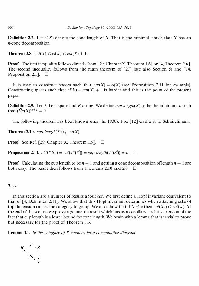
Lemma 3.1. In the category of R modules let a commutative diagram


and a map r :>PX be given. Assume that pr"id, pf @"f, im(rf )Lim( f @ ) and that f is injective. Thenrf"f @.

Proof. For any a3M there is a b such that rf (a)"f @(a)#f @(b). So pr f (a)"pf @(a)#pf @(b). Sopf @ (b)"0. So b"0. h

Lemma 3.2. Let f :XP> be a map such that conX*r and con f*s*r. ThenconF

n( f )*nr#s#n!1.

Proof. Follows from Lemma 2.4. h

Lemma 3.3. Let

be a map between two short exact sequences of abelian groups. Assume that f and h are surjections.Then g is a surjection and p induces a surjection ker(p)Pker(h).

Proof. Clear. h

De5nition 3.4. Let X be a space such that cat(X))nO0 and r : XPGnX a homotopy section of

pn. Let f3[R=,X]. Let Rf a also denote the map inclusion "Rf a : R=PG

1(X)PG

n(X). De"ne the

Hopf invariant of f byHr( f )"Rf a!rf. Since pRf aKfKpr f we can, and will, considerH

r( f ) to be

in [R=,Fn(X)].

Observe that the class Hr( f ) is uniquely determined since the map XF

n(X)PXG

n(X) has

a retraction. Also the map Rf a :R=PG1(X) is actually the suspension of the adjoint R=PRXX

composed with the homotopy equivalence RXXPG1(X). See [26] for more details. The fact that

this is in fact equivalent to the Berstein}Hilton Hopf invariant when= is a sphere has been provedby Iwase [19].

Some version of the following theorem was also known to Halperin, Iwase [19] and perhapsothers. It improves on a result of Cornea [6] which states that cat(X

n))cat(X)#1. He conjec-

tured that this improvement could be made. It follows that the main result of the same paper can beimproved by one in the in"nite case.

Theorem 3.5. Let X be a connected but not necessarily simply connected CW-complex, cat(X)"n'0and r :XPG

nX be a section. Then there are compatible sections r

s: X

sPG

nX

sof the Ganea xbration

ps: G

nX

sPX

s.

Proof. Assume that we have already de"ned the compatible sections for s(l.


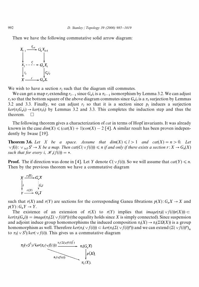
Then we have the following commutative solid arrow diagram:

We wish to have a section rlsuch that the diagram still commutes.

We can get a map rlextending r

l~1since G

nilis a n

l~1isomorphism by Lemma 3.2. We can adjust

rlso that the bottom square of the above diagram commutes since G

nilis a n

lsurjection by Lemmas

3.2 and 3.3. Finally, we can adjust rl

so that it is a section since pl

induces a surjectionker(n

lG

nil)Pker(n

lil) by Lemmas 3.2 and 3.3. This completes the induction step and thus the

theorem. h

The following theorem gives a characterization of cat in terms of Hopf invariants. It was alreadyknown in the case dim(X))(cat(X)#1)con(X)!2 [4]. A similar result has been proven indepen-dently by Iwase [19].

Theorem 3.6. Let X be a space. Assume that dim(X))l'1 and cat(X)"n'0. Letsf(i) :s

i|ISlPX be a map. Then cat(C(sf (i))))n if and only if there exists a section r : XPG

n(X)

such that for every i, Hr( f (i))"*.

Proof. The if direction was done in [4]. Let > denote C(sf (i)). So we will assume that cat(>))n.Then by the previous theorem we have a commutative diagram

such that r(X) and r(>) are sections for the corresponding Ganea "brations p(X) :GnXPX and

p(>) :Gn>P>.

The existence of an extension of r(X) to r(>) implies that image(nl((sf (i))r(X)))L

ker(nl(G

ni))"image(n

l(R(sf (i))a)) (the equality holds since X is simply connected). Since suspension

and adjoint induce group homomorphisms the induced composition nl(X)Pn

l(RX(X)) is a group

homomorphism as well. Therefore ker(nl(sf (i)))Lker(n

l(R(sf (i))a)) and we can extend (R(sf (i))a)

Hto n

l(sSl)/ker(sf (i)). This gives us a commutative diagram


Together with the map r(X)H

we then have the setup of Lemma 3.1. So we can conclude thatnl(r(X)sf (i))"n

l(R(sf (i))a) and hence also the theorem. h

Lemma 3.7. Let b : SlPSr be a coH map, f : SrPX any map and s :XPGn(X) a section of the Ganea

xbration. Then Hs( fb)"H

s( f )b.

Proof. The lemma follows since R( fb) a"Rf ab if b is coH. h

Lemma 3.8. Let b :SrPSn be a coH map. Let f : SnPX be any map. Then XsSnXb er`1K(XsSn)Xb`fb er`1. Therefore if XK. * cat(XsSn)Xb`fb er`1"catX and if clX*2 thencl (XsSnXb`fb er`1))clX.

Proof. Clear. h

Note that if b is not a coH map then the previous two lemmas will generally not be true. For anexample take b"[n, n] : S15PS8 and f"[n

1, n2, n3] : S8P¹3(S3).

The next proposition and its proof were pointed out to me by Howard Marcum. More generalstatements can be found in [8, Section 6].

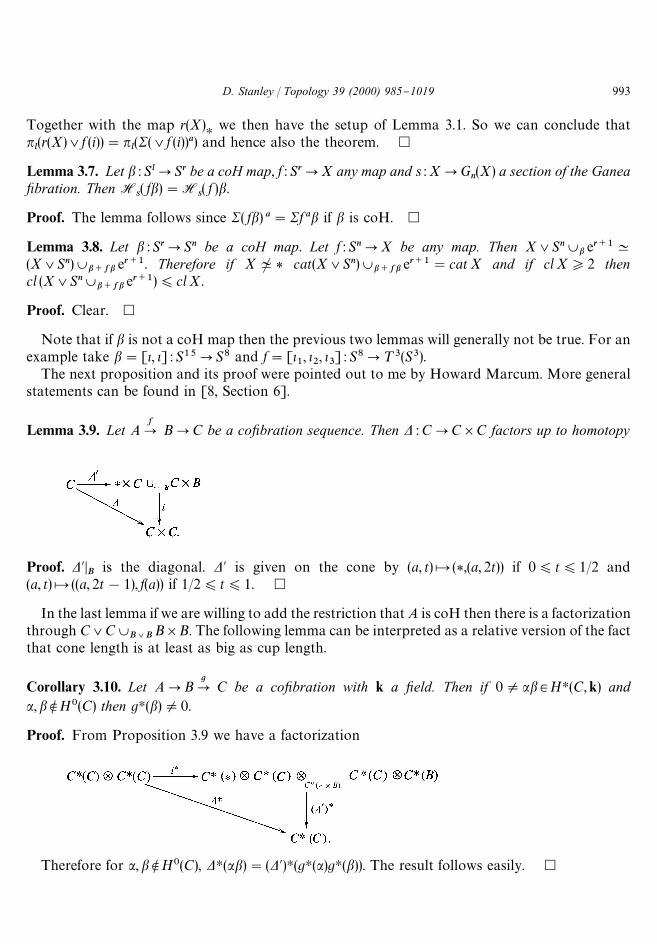
Lemma 3.9. Let A fP BPC be a coxbration sequence. Then D : CPC]C factors up to homotopy

Proof. D@DB

is the diagonal. D@ is given on the cone by (a, t)C (*,(a, 2t)) if 0)t)1/2 and(a, t)C ((a, 2t!1), f(a)) if 1/2)t)1. h

In the last lemma if we are willing to add the restriction that A is coH then there is a factorizationthrough CsCX

B[BB]B. The following lemma can be interpreted as a relative version of the fact

that cone length is at least as big as cup length.

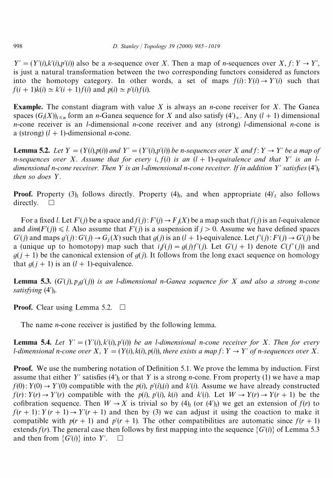
Corollary 3.10. Let APB gP C be a coxbration with k a xeld. Then if 0Oab3HH(C,k) and

a,b NH0(C) then gH(b)O0.

Proof. From Proposition 3.9 we have a factorization

Therefore for a,b NH0(C), DH(ab)"(D@)H(gH(a)gH(b)). The result follows easily. h


We also have the dual result which is a relative version of cocup length being a lower bound forcategory.

Corollary 3.11. Let APB gP C be a coxbration sequence. Let x3H

H(C). If there exists

0Ox@i3H

H(C) and linearly independent xA

i3H

H(C) such that DM x"R

ix@i?xA

ithen there exists

y3HH(B) such that xA

i"g(y).

Proof. Use the dual of the proof of the last corollary. h

4. r-cone decompositions

In this section we construct spaces Q such that cat(Q)"r and cl(Q]Sn)"r for large n. Since cl isan upper bound for cat this also shows that cat(Q)"cat(Q]Sn) thus giving an alternative (to [18])proof that there are counterexamples to Ganea's conjecture. Using Iwase's method we also showthat for n one less, cat(Q]Sn)"r.

For this section let r,l*2 and s'rl. Let b :Ss~1PSrl~1 be any map. Let w : Srl~1P¹r(Sl)denote the higher-order Whitehead product in other words the attaching map of the top cell in theproduct. Let Q"¹r(Sl)X

wb es.

Theorem 4.1. If RnbaK* then cl(Q]Sn)"r.

Proof. cup length(¹r(Sl))"r!1. Since s'lr, b is trivial on HH and so cup length(Q)*r!1. Wesee that r)cup length(Q]Sn))cat(Q]Sn))cl(Q]Sn). (The "rst inequality is straightforwardand the second and third follow from Theorem 2.10 and Proposition 2.8.) Next, we will show thatcl(Q]Sn))r.

Let Z"¹r(Sl)X(¹r(Sl)(r~2)l

]Sn). Since ZsR(XSrl~1Xba es~1) has cone length r!1, it is enoughto construct a co"bration sequence :

=PZsR(XSrl~1Xba es~1)PZ@ (#)

such that Z@KQ]Sn.From Lemma 2.1 there exists a co"bration sequence (*) :

(XSrl~1Xba es~1) * Sn~1 w{P R(XSrl~1Xba es~1)sSn

pP R(XSrl~1Xba es~1)]Sn.

Let e :RXSrl~1PSrl~1 denote the evaluation. Let i(1) :RXSrl~1PR(XSrl~1Xbaes~1), i(2) :Srl~1PSrl~1Xb es and i(3) :ZPZsR(XSrl~1Xba es~1) denote the inclusions. There is a homotopy pushout


and a co"bration sequence

Srl~1w`i(2)&" ¹r(Sl)sSrl~1Xb esPQ.

These two facts imply that

RXSrl~1we`i(1)&" ¹r(Sl)sR(XSrl~1Xba es~1)PQ (##)

is a co"bration sequence.There exists f @ and a homotopy commutative diagram (**):

g is an Hs

surjection and so g]id is an Hs`n

surjection. Let d : HH(R(XSrl~1

Xba es~1)]Sn)PHH~1

((XSrl~1Xba es~1) * Sn~1) denote the connecting homomorphism. Leth : Ss`n~1P(XSrl~1Xba es~1) *Sn~1 be a map such that H

H(g]id )d~1H

H(h) surjects onto

Hs`n

(Q]Sn) (h is just the sphere corresponding to es~1 * Sn~1 which has trivial attaching map sinceRnbaK*).

We can now construct our sequence (#). Let; be a wedge of spheres and f :;PZ a map suchthat C( f )K¹r(Sl)]Sn. Let

h"i(3) f#(we#i(1))#f @h :;sRXSrl~1sSs`n~1PZs(XSrl~1Xba es~1)

We show that there is a map C(h)PQ]Sn that is an HH

equivalence. From the fact thatC( f )K¹r(Sl)]Sn and from (##) we get a map C ( f#(we#i(1))PQ]Sn. This is an H

Hisomor-

phism except in dimension s#n. Since (**) commutes we get an extension C(h)PQ]Sn which isan H

Hisomorphism. We thus have our sequence (#). So we see that r*cl(Q]Sn)*cup-

length(Q]Sn)*r. So cl(Q]Sn)"r. h

It is, in fact, the breakdown of the proof of the previous theorem when RnbaK. * that points us inthe direction of the examples we are seeking. Essentially, we will use the fact that we have noco"bration sequence of the form (*) in the proof of the theorem to show we cannot have any r-conedecomposition of Q]Sn. Since RnbaK. * a certain homology class is not in the image of Hurewicz.But any r-cone decomposition can be adjusted to show that that homology class must be in theimage of Hurewicz.

The following lemma is similar to [4, Proposition 2.5]. As is standard Ml(p) denotes the Moorespace with H

l(Ml(p),Z)"Z/p.


Lemma 4.2. pr~1

: Gr~1

(¹r(Sl))P¹r(Sl) has a unique (up to homotopy) section s and s is compatiblewith any section s@ of p

r~1: G

r~1(¹r(Ml(p))P¹r(Ml(p)).

Proof. By Theorem 2.4 con(Fr~1

(¹r(Sl)))"con(Fr~1

(¹r(Ml(p))))"r(l!1)#(r!1)!1"rl!2.Since dim(¹r(Sl))"(r!1)l and l*2 the lemma follows. h

Theorem 4.3. Let b be a coH map. If r"2 assume b is a suspension. Then catQ"r if and only ifbK. * otherwise catQ"r!1. If RnbK* then cat(Q]Sn)"r.

Proof. Let i : SlPMl(p) be the inclusion. Let s :¹r(Sl)PGr~1

(¹r(Sl)) and s@ :¹r(Ml(p))PG

r~1(¹r(Ml(p))) be sections of the corresponding Ganea "brations. By Lemma 4.2 the sections are

compatible with ¹r(i) and Gr~1

(¹r(i)). So for every s@, Hs{(¹r(i)w)"*r~1Xi(H

s(w)). Now we see

using cup length for HH(},Z/p) that cat(¹r(Ml(p))XT

r(i)werl)"r. Therefore H

s{(¹r(i)w)O*. But

since con(*r~1X¹r(Ml(p)))"lr!2, Hs(w) is nontrivial and in fact is not p divisible. The fact that

X¹r(Sl) is a product of spheres together with Lemma 3.7 then imply the "rst statement in thetheorem.

To prove the second part we use a variant of the method of Iwase. This method arose indiscussions with Octavian Cornea. Remember Cyl(X)+X'I` is just the reduced cylinder on X.We have a strictly commuting diagram such that the rows are co"bration sequences.

Where i is the inclusion into the end of the cylinder and j and f are the inclusions. The map onCylSs~1 is the homotopy between wb and jb given by the s-cell in the image space.

So using Lemma 2.1 we get another strictly commuting solid arrow diagram such that the rowsare co"brations.

Since b * Sn~1"RnbK* there exists h such that hpK( f]Sn)Xid

id. By an easy HH calculationp@h is a weak equivalence. Now it follows from Lemma 3.8 that (Slr~1s¹r(Sl))X

(j~w)b%sKSlr~1Xb ess¹r(Sl). (If r"2 it is here that we use that b is a suspension.) So it iseasy to see that cl((Slr~1s¹r(Sl)Xes)]SnXQ))r. Therefore cat(Q]Sn))r. h

We can now use the results of Gray [16] (Corollary 9.2) to see that at every prime p'2 andevery r,n there exists Q such that cat(Q)"r, cat(Q]S2n~1)"r and cl(Q]S2n)"r. It also follows


from results of Iwase [18] or Vandembroucq [28] that if R2n~2bO* then cat(Q]S2n~2)"r#1.In the next few sections we will build up the machinery to show that in many casescl(Q]S2n~1)"r#1.

5. Ganea sequences and n-cone receivers

In this section we introduce n-cone receivers (De"nition 5.1). They are the main tool we use totransform general n-cone decompositions into more manageable sequences of spaces. We provesome lemmas for constructing n-cone receivers out of other ones. We also introduce Ganeasequences. The notion of Ganea sequence is related to the LS "brations of Scheerer}TanreH [25].

Fix 0)n)R. Let X be a space. For 0)i)n let >(i) be spaces and k(i) :>(i)P>(i#1) andp(i) :>(i)PX be maps such that p(i)"p(i#1)k(i). We call>"(>(i),k(i),p(i)) an n-sequence over X.In other words, it is just a functor from the poset of the ordinal n to the homotopy category ofspaces over X. Let 0)l)R.

Consider the following properties :

(1) >(0)"*.(2)

lk(i) is attaching a cone on a space of dimension at most l.

(2')l

for i'0 k(i) is attaching a cone on a suspension of a space of dimension at most l!1.(3)

lFor every = of dimension less than or equal to l and i*1, [R=, p(i)] is surjective.Equivalently for every i*1, Xp(i) splits up to (XX)

l. In other words, for any CW-structure on

XX there exists a commutative diagram.

(4)l

For every= of dimension less than l and i*1, ker[R=, k(i)]"ker[R=,p(i)]. Equivalentlyfor every i*1 and any CW-structure the induced map (XFib(p(i)))

l~1PX>(i#1) is trivial.

(4')l

For every = of dimension less than or equal to l and i*1, ker[=, k(i)]"ker[=, p(i)] orequivalently for every i*1, the induced map Fib(p(i))

lP>(i#1) is trivial.

Notice that (4)=

is equivalent to requiring that the induced map XFib(p(i))PXFib(p(i#1)) isinessential.

De5nition 5.1. We call an n-sequence over X an l-dimensional n-cone over X if it satis"es (1) and(2)

land an l-dimensional strong n-cone over X if it satis"es (1), (2)

land (2@)

l. We call an n-sequence

over X an l-dimensional n-cone receiver for X if it satis"es (3)land (4)

l. We call an n-sequence over

X an l-dimensional n-Ganea sequence for X if it satis"es (1), (2)l, (3)

land (4)

l.

In all of these cases we will (ab)use the notation M>(i)N or (>(i),p(i)) if the maps are clear from thecontext. Also if l"R we will often drop the pre"x l-dimensional from our de"nitions. Let


>@"(>@(i),k@(i),p@(i)) also be a n-sequence over X. Then a map of n-sequences over X, f :>P>@,is just a natural transformation between the two corresponding functors considered as functorsinto the homotopy category. In other words, a set of maps f (i) :>(i)P>@(i) such thatf (i#1)k(i)Kk@(i#1) f (i) and p(i)Kp@(i) f (i).

Example. The constant diagram with value X is always an n-cone receiver for X. The Ganeaspaces (G

i(X))

ixnform an n-Ganea sequence for X and also satisfy (4@)

=. Any (l#1) dimensional

n-cone receiver is an l-dimensional n-cone receiver and any (strong) l-dimensional n-cone isa (strong) (l#1)-dimensional n-cone.

Lemma 5.2. Let>"(>(i),p(i)) and >@"(>@(i),p@(i)) be n-sequences over X and f :>P>@ be a map ofn-sequences over X. Assume that for every i, f (i) is an (l#1)-equivalence and that >@ is an l-dimensional n-cone receiver. Then> is an l-dimensional n-cone receiver. If in addition >@ satisxes (4@)

lthen so does >.

Proof. Property (3)l

follows directly. Property (4)l, and when appropriate (4)@

lalso follows

directly. h

For a "xed l. Let F@( j) be a space and f ( j) : F@(j)PFj(X) be a map such that f ( j) is an l-equivalence

and dim(F@( j)))l. Also assume that F@( j) is a suspension if j'0. Assume we have de"ned spacesG@( j) and maps g@( j) : G@( j)PG

j(X) such that g( j) is an (l#1)-equivalence. Let f @( j) : F@( j)PG@( j) be

a (unique up to homotopy) map such that ijf ( j)"g( j) f @( j). Let G@( j#1) denote C( f @ ( j)) and

g( j#1) be the canonical extension of g( j). It follows from the long exact sequence on homologythat g( j#1) is an (l#1)-equivalence.

Lemma 5.3. (G@( j), pjg@( j)) is an l-dimensional n-Ganea sequence for X and also a strong n-cone

satisfying (4@)l.

Proof. Clear using Lemma 5.2. h

The name n-cone receiver is justi"ed by the following lemma.

Lemma 5.4. Let >@"(>@(i), k@(i),p@(i)) be an l-dimensional n-cone receiver for X. Then for everyl-dimensional n-cone over X, >"(>(i), k(i), p(i)), there exists a map f :>P>@ of n-sequences over X.

Proof. We use the numbering notation of De"nition 5.1. We prove the lemma by induction. Firstassume that either >@ satis"es (4@)

lor that > is a strong n-cone. From property (1) we have a map

f (0) :>(0)P>@(0) compatible with the p(i), p@(i),(i) and k@(i). Assume we have already constructedf (r) :>(r)P>@(r) compatible with the p(i), p@(i), k(i) and k@(i). Let =P>(r)P>(r#1) be theco"bration sequence. Then =PX is trivial so by (4)

l(or (4@)

l) we get an extension of f (r) to

f (r#1) :> (r#1)P>@(r#1) and then by (3) we can adjust it using the coaction to make itcompatible with p(r#1) and p@(r#1). The other compatibilities are automatic since f (r#1)extends f (r). The general case then follows by "rst mapping into the sequence MG@(i)N of Lemma 5.3and then from MG@(i)N into >@. h


The previous lemma has as a corollary that any n-Ganea sequence can be used to de"ne LScategory. Essentially, the same lemma was proved by Scheerer}TanreH [25].

Corollary 5.5. Let (>(i), k(i), p(i)) be an n-Ganea sequence for X. Then cat(X))n if and only if p(n) hasa homotopy section.

Proof. Compare the sequence to the Ganea spaces Gn(X). h

Next, we give a few lemmas concerned with constructing cone receivers out of other ones.

Lemma 5.6. Let >"(>(i), k(i), p(i)) be an l-dimensional n-cone receiver for X. Then for any=, >]="(>(i)]=,k(i)]id, p(i)]id) is an l-dimensional n-cone receiver for X]=.

Proof. Clear. h

We do not use the following lemma but include it nonetheless.

Lemma 5.7. Let > be a n-cone receiver for X. Then for every =, >s="

(>(i)s=,k(i)sid,p(i)sid) is a n-cone receiver for Xs=.

Proof. Consider the following diagram where the rows and columns are "bration sequences andj and j@ are the inclusions.

Since Xp(i) has a section we know that for some XF(i), X>(i)KXX]XF(i). So

X>(i) *X=KXX*X=sRXF(i)'X=sRXX'XF(i)'X= (*).

Since the map F(i)PF(i#1) induced by >(i)P>(i#1) is trivial, we see that the induced map onthe second and third factors of the wedge decomposition (*) is trivial also. This implies that theinduced map F@(i)PF@(i#1) is trivial. By assumption the map F(i)PF(i#1) is trivial afterlooping. Xj and Xj@ have compatible sections. So XFA(i)KXF(i)]XF@(i) and the mapFA(i)PFA(i#1) must be trivial after looping. h

Lemma 5.8. Let


be a commutative diagram where p and p@ denote the projections. Then the induced mapFib(p)PFib(p@) is trivial.

Proof. Factor through id : APA. h

The next three lemmas show that certain well known equivalences are natural.

Lemma 5.9. Let f :XP> be a map. Then for every A there exists a homotopy commutative diagram inwhich the horizontal arrows are weak equivalences.

Proof. Consider the following homotopy pushout.

Next quotient out each corner by X. The proposition follows since we see that XIRAKR(XIA)in a natural way. h

Lemma 5.10. Let a commutative diagram with the rows xbration sequences be given.

Assume that B and B@ are H-spaces and that g is an H-map. Assume there exists maps r : CPB andr@ : C@PB@ such that prKidKp@r@ and grKr@h. Then there exists a homotopy commutative diagram

such that the horizontal maps are weak equivalences.


Proof. Use the standard argument with the long exact sequence on nH

comparing the given"bration with the product "bration. h

Lemma 5.11. Let

be a commutative diagram such that the rows are coxbration sequences and h is the induced mapbetween the coxbres. Assume that there exist homotopy sections s(i) of Xf(i) such that Xgs(1)Ks(2)Xh.Then there exists a commutative diagram

such that the horizontal arrows are weak equivalences and l is the induced map between the xbres.

Proof. Since h is the induced map between co"bres the cube axiom gives us homotopypushouts

and a homotopy commutative diagram

h(i)DXC(i) is the connecting map. (This can be seen by taking the cubes and adding a layer aboveby taking homotopy "bres of the vertical maps.) The fact that the s(i) are compatible means thatthe homotopies h(i)DXC(i)K* are compatible. (Since they both are induced from the natural


homotopy of the composition XB(i)PXC(i)PFib( f (i)) to *.) So we get a homotopy commutativediagram

in which the horizontal arrows are weak equivalences. The lemma then follows from Lemma 5.9.h

The map f in the next lemma would appropriately be called a homotopy inert map [2,17]. Thelemma then says that we can construct r-cone receivers for spaces with inert homotopy classes byconstructing r-cone receivers for the cone on the homotopy inert map. It is the most interesting ofour series of lemmas constructing r-cone receivers out of other ones.

Lemma 5.12. Let r*2. Let f : SnPX be a map and let g : XPC( f ) denote the inclusion. Let > be anr-sequence over X such that (>(i),k(i),gp(i)) is an r-cone receiver for C( f ). Assume that for everyi(r, X(p(i)j(i)) : XG(i)PX>(i)PXX is inessential. Then >sSn"(>(i)sSn,k(i)sid,p(i)#f ) is ar-cone receiver for X.

Proof. Throughout the proof / will denote the loop multiplication on any loop space. Consider thefollowing homotopy commutative diagram:

in which the rows and columns are "bration sequences and the bottom right square strictlycommutes. (So that we can use Lemma 5.11.)

Let s :XC( f )PX>(1) be a section of Xgp(1). We will also let it denote the sections XC( f )PX>(i)obtained by composing s with the k(i).

For every i let s@(i) :>(i)P>(i)sSn be the inclusion map and s(i)"Xs@(i) if i(n. Lett"X(p(1)#f )Xs@(1)s. It is easy to see that t is a section of Xg. Consider the diagram

(*)


Since Xp(i)j(i)K* if iOr making the map in the "rst row Xj(i)]s or *]s gives homotopiccompositions into XX. Therefore,

X(p(i)#f )s(i)KtX(gp(i)) (1)

for every i(n and

X(k(i)sid)s(i)Ks(i#1)Xk(i) (2)

for every i(n!1. (Note that (2) would hold for i"n!1 if s(n) were Xs@(n).)Since r*2 (1) holds for i"1 and so Lemma 5.11 implies that p@(i) : F(1)PF is equivalent to the

projection

idsid#*#* : SnsSn'XC( f )sXG(1)sSn'XG(1)PSnsSn'C( f ).

Let r be a section of this projection. Then since t and s(1) are compatable Xr]s induces a section s@of X(p(1)#f ) by Lemma 5.10. Again we will also denote the composition of s@ with the k(i) by [email protected] we have not assumed XG(r)PXX is inessential we cannot use s(r)"Xs@(r). We have to adjustit slightly. Let

s(r)"/((X(s@(r) j (r))!s@X(p(r) j (r)))](Xs@(r)s)) : XG(r)]XC( f )PX(>(r)sSn),

where ! refers to inverse composed with loop multiplication. (p(r)#f )s@(r)Kp(r). SoX(p(r)#f )(X(s@(r)j(r))!s@X(p(r)j(r)))KX(p(r)j(r))!X(p(r)j(r))K*. Therefore,

X(p(r)#f )s(r)KtX(gp(r)) (3)

and by an argument similar to the one above involving the diagram (*)

X(k(r!1)sid)s(r!1)Ks(r)Xk(r!1). (4)

We next show that s(r) is a section of Xn(r). Since gp(r)j(r)K*, p(r)j(r) factors through F. Sos@X(p(r)j(r)) factors through XF(r). Therefore, Xn(r)s@X(p(r)j(r))K*. So Xn(r)(X(s@(r)j(r))!s@X(p(r)j(r)))KXn(r)X(s@(r)j(r))KXj(r). Also Xn(r)Xs@(r)sKs. It follows that s(r) is a section of Xn(r).

Let Z(i) denote SnsSn'XC( f )sXG(i)sSn'XG(i). Using (1)}(4) and Lemma 5.11 we see that thetriangle

is equivalent to the triangle

where the maps are the induced maps between the "bres. It follows that the induced mapH(i)PH(i#1) is inessential.


Since the sections t, s(i) and s(i#1) are compatible there exists compatible sectionss@(i) : XG(i)PXG@(i) of h(i). So since we know that the map XG(i)PXG(i#1) induced by k(i) isinessential we can apply Lemma 5.10 to see that the map G@(i)PG@(i#1) induced by k(i)sid isinessential. h

The next lemma says that if we have any r-cone receiver for any space, we can construct anr-cone receiver for that space with another cell attached.

Lemma 5.13. Let (>(i), k(i), p(i)) be a r-cone receiver for X and assume that >(i) and X aren-connected. Let s : XXPX>(1) be a section of Xp(1). Let f :SlPX be a map. Denote g(1)"sf andg(i)"k(i)g(i!1). Let >@(0)"> and for i'0 >@(i)"C(g(i)). Let k@(i) and p@(i) be the canonicalextensions. Then (>@(i), k@(i), p@(i)) is an l#n!1-dimensional r-cone receiver for C( f ).

Proof. Use the Serre exact sequence to show that Fib(p(i))PFib(p@(i)) is an (l#n!1)-equivalence.It is also easy to construct a section of Xp@(i) up to dimension l#n!1 which extends s. h

It seems likely that the number l#n!1 in the last lemma can be improved to l#2n!1.

6. Eilenberg}Moore spectral sequence

The main object of this section is to construct an n-cone receiver for a product of spheres(Lemma 6.10). To do this we calculate the "bre of the inclusion of a skeleton into the product andthe induced map between such "bres. The method is to calculate the homology of the "bres and theinduced maps on homology using the relative cobar construction. The primary reference for thissection is [10].

Throughout this section we work over R"Z/p or Z(p)

. All spaces with be p local. HH(}) denotes

HH(}, R) and Cs

H(}) denotes singular chains with R coe$cients. Let DGC denote the category of

connected di!erential graded coalgebras over R. We will also refer to the objects (maps) in DGC asDGCs (maps of DGCs). For a "nite type A3DGC, AH denotes the dual di!erential graded algebra.(For our purposes it is enough to consider DGCs that are "nitely generated as R modules in eachdegree.) For a map APB in DGC recall the de"nition of X(A;B) and B(AH;BH) from [10]. EMSSdenotes the Eilenberg}Moore spectral sequence. The following is one of the main theorems of [10].

Theorem 6.1 (Felix et al. [10]). Let f :XP> be a map. Let CsH(X) have the Cs

H(>) comodule structure

coming from f. Then X(CsH(X),Cs

H(>)) and Cs

H(Fib( f )) are naturally weak equivalent.

Lemma 6.2 (Felix et al. [10]). Let A,A@,B, B@ be projective as R modules. In DGC assume we havea commutative diagram


such that f and g are weak equivalences. Then the induced map X(A; B)PX(A@;B@) is a weakequivalence.

The last lemma leads naturally to the next de"nition.

De5nition 6.3. Let f : APB be a map in DGC and assume that HH(A) and H

H(B) are projective

R modules. We call f formal if we have a commutative diagram

such that all the vertical maps are weak equivalences and all the underlying R modules areprojective. A DGC, B is called formal if id : BPB is formal.

Lemma 6.4. The Eilenberg}Zilber map, EZ : CsH(A)?Cs

H(B)PCs

H(A]B), is a map in DGC.

Proof. See Eilenberg and Moore [9, Section 17]. h

Lemma 6.5. Let X be a CW-complex such that CH(X) has trivial diwerential. Assume Cs

H(X) is a formal

DGC. Then for every r, CsH(i) : Cs

H(X

r)PCs

H(X) is formal.

Proof. Observe that CsH(X

r)PCs

H(X) is split injective as R modules. Let h : Cs

H(X

r)rPCs

H(X

r) be

a subDGC of CsH(X

r) such that h is a graded R module isomorphism in gradings less than r, such

that CsH(X

r)ris 0 in gradings greater than r#1 and such that h induces an H

Hisomorphism. We can

extend h to h@ :CsH(X)

rPCs

H(X) a subDGC of Cs

H(X) such that h@ is a graded R module isomorphism

in gradings less than or equal to r, such that H(CsH(X)

r) is 0 in gradings greater than r and such that

h@ induces an HH

isomorphism for *)r.

So we have a commuting solid arrow diagram:


such that h, g and h are weak equivalences. Since h@ is an isomorphism in gradings less than or equalto r and C

H(X) has trivial di!erential there exists a weak equivalence f making the diagram

commute. The conclusion of the lemma follows directly. h

Lemma 6.6. The inclusion CsH(Sl)n

rlPCs

H(Sl)n

slis formal for every r)s.

Proof. CsH(Sl) is formal and the tensor product of two formal DGCs is formal. Therefore the lemma

follows from the last two lemmas. h

Lemma 6.7. Let

be a diagram in DGC with all maps formal. Then the induced map HX(A;B)PHX(C;D) is the sameas the induced map (interpreted as composed with the isomorphisms of Lemma 6.2)HX(H

HA; H

HB)PHX(H

HC;H

HD).

Proof. The identi"cation follows from Lemma 6.2. h

For the next three lemmas let F(r) denote the "bre of the inclusion ((Sl)n)lrP(Sl)n. The "rst two

calculate the homology of these "bres and the induced map between them. Since all the maps weare dealing with are formal this calculation is made easier by the last lemma. We work dually withthe bar construction. We will use spectral sequence notation since we also have the E

1term of an

EMSS.

Lemma 6.8. Let r*1. Let Es`1,H1

"HI H((Sl)n)s?HH(((Sl)n)lr) be the weight s#1 part of

B(HH((Sl)nlr),HH((Sl)n))KCH(F(r)). Then in H(B(HH((Sl)n

lr),HH((Sl)n))) we can represent all elements by

sums of elements of the form a(1)?2?a(s)?b. Where a(i)3HI H((Sl)n) are indecomposable andb3HH(((Sl)n)

lr) has product length r.

Proof. Let a3ZH(Es`1,H

1). Grade Es`1,H

1left lexicographically by cohomological product length

and assume that a is in the minimal gradation. There are two cases. In the "rst case some of theelements in HI H((Sl)n) are decomposable and in the second case all are indecomposable. We showthat the "rst case cannot occur and then derive the lemma in the second case.

Case (1): In this case there exist integers t and q, indecomposables a(k, i, j)3HH((Sl)n), homogene-ous decomposables b(i, j)3HH((Sl)n), a lower order term d and linearly independent c( j)3Eq,H

1such

that

a"+i,j

a(1, i, j)?2?a(t, i, j)?b(i, j)?c( j)#d.


Observe that da"0 modulo terms of gradation lower than a(1, i, j)?2?a(n, i, j)?b(i, j)?c( j). Soin fact for every j

Z(i)"+i

a(1, i, j)?2?a(t, i, j)?b(i, j)

is a cycle. But since the b(i, j) are decomposable there is an x( j) such that d(x( j))"z( j). (This can beseen either directly or by looking at the EMSS converging to the homology of the "bre of *P(Sl)n.)So a is homologous to a!+

j(x( j)?c( j)) which is an element in a lower gradation. This is

a contradiction. So we must have:Case (2): There exists b(i, j)3HH(((Sl)n)

lr) of product length j)r and indecomposables

a(k, i, j)3HI H((Sl)n) such that

a"+i,j

a(1, i, j)?2?a(s, i, j)?b(i, j).

But then observe that

u" +i,j:r

a(1, i, j)?2?a(s, i, j)?b(i, j)

is a cycle and a@"a!d(u?1) is a cycle satisfying the properties required by the lemma. h

Now to calculate the induced map on homology between the "bres we do not have the problemof dealing with associated graded modules. This is another advantage of this approach over usingthe EMSS directly.

Lemma 6.9. With the notation given before the statement of the last lemma, the induced mapF(r)PF(r#1) is trivial on H

H.

Proof. For "nite type A,B3DGC, (X(A,B))H"B(AH,BH). Therefore by Theorem 6.1, Lemmas 6.6and 6.7, Lemma 6.8 gives generators of HH(F(r#1)). The map is trivial since all the representativecycles described in Lemma 6.8 go to 0 in B(HH((Sl)n

lr),HH((Sl)n)). Dualizing, we get the desired

result. h

Theorem 6.10. Let k(r) : (Sl)nrlP(Sl)n

(r`1)land p(r) : (Sl)n

rlP(Sl)n be the inclusions. Then ((Sl)n

rl,k(r),p(r)) is

an n-Ganea sequence for (Sl)n. Also each F(r) is a wedge of spheres.

Proof. It is clear that > is an n-cone over (Sl)n and that Xp(1) has a section. So it is su$cient toverify that the induced map F(r)PF(r#1) is trivial. Let s

IS(r`1)l~1P(Sl)n

rlP(Sl)n

(r`1)lbe a co"b-

ration sequence. Then from the cube axiom (Theorem 2.2) we get a homotopy push out:


Since Xp(r) splits h is trivial on the "rst factor of the product. Also AISiSniK(AsS0)'(S

iSni).

Therefore we get a co"bration sequence:

(X(Sl)nsS0)'sIS(r`1)l~1 f

P F(r) gP F(r#1).

But since we know from Lemma 6.9 that HH(g)"0, H

H( f, Z/p) and H

H( f, Z

(p)) are both surjections.

But then the fact that the "rst term in the sequence is a "nite type wedge of spheres implies that F(r)is a wedge of spheres and gK*. h

The calculation of the "bres F(r) is a special case of Porter [23]. He uses geometric techniques.However he does not, at least explicitly, give the map between the "bres. In our special case this wasdone in Lemma 6.9 and Theorem 6.10. It seems that the methods of this section could be used torecover the result in Porter's generality.

7. Changing cone decompositions

In this section we start with an arbitrary cone decomposition of our space Q]Sn and derivea co"bration sequence with speci"c properties (Lemma 7.8). This is done in three steps. First, weapply the results of the last two sections to get an (s#l!3)-dimensional (r!1)-cone receiver forQ]Sn (Lemma 7.1). Next, we show that any r-cone decomposition for Q]Sn can be assumed to be(n#s!2)-dimensional up to the (r!1)st stage (Lemma 7.6). Putting these two facts togetherallows us to map our cone decomposition into our cone receiver. We then construct our desiredco"bration sequence by pinching out some skeleton of the penultimate stage of the r-cone receiver(Lemma 7.8). We designed our receiver speci"cally to "t the results of Lemma 7.8. It had to be smallenough to manipulate easily but close enough to the Ganea spaces to contain the obstruction thatwe need in the next section. Along the way to Lemma 7.8 we prove two results about restricting theform of general cone decompositions (Lemmas 7.3 and 7.4).

Let Q, b, r, l and s be as in Section 4. Let X(i)"(Sl)rlisSlr~1Xb es. Let k@(i) : X(i)PX(i#1) be

the inclusion. Let p@(i) :X(i)PQ be the map that is the inclusion on (Sl)rli, w on Srl~1 and the

canonical extension over es. We "x a prime p and work with p-local spaces.

Lemma 7.1. (X(i)]Sn, k@(i)]id,p@(i)]id) is an (s#l!3)-dimensional (r!1)-cone receiver forQ]Sn.

Proof. Let p(i) : (Sl)nliP(Sl)n be the inclusion. It follows from Theorem 6.10 that for every

i(n!1, Fib(p(i))P¹n(Sl) is trivial. So if r'2 that MX(i)N is an (s#l!3)-dimensional (r!1)-cone receiver for Q follows by using, in succession (Theorem 6.10, Lemmas 5.12 and 5.13). If r"2the fact that MS2l~1,SlsSlsS2l~1N is a 1-cone receiver of SlsSl follows directly from thede"nitions so we only need to use Lemma 5.13. The conclusion of the lemma then follows fromLemma 5.6. h

Lemma 7.2. Let A be a space of dimension n such that Hn(A) is torsion free and let B be simplyconnected. Let f : APB be a map that is trivial on H

n. Then f factors through B

n~1.


Proof. The factorization through Bnfollows from cellular approximation. Observe that a factoriz-

ation can be chosen preserving the assumption on Hn( f ). Next the assumption implies that the

composition of f with p :BnPB

n/B

n~1is trivial. The result then follows since the Serre exact

sequence implies that Bn~1

PFib(p) is n-connected. h

The next two lemmas are technical but very easy to accept as true without reading their proofs.The author would never encourage this.

Lemma 7.3. Let M>(i)N be an r-cone decomposition for >. Assume that > is simply connected. Thenthere is a strong r-cone decomposition of >, M>@(i)N such that for every i, >@(i) is simply connected.

Proof. Replace M>(i)N by an r-cone decomposition for >, M;(i)N such that we have co"brationsequences

Ri=(i)f(i)P;(i)P;(i#1).

Cornea [5, Theorem 1.1] proves that this can be done. In particular this implies that for everyi'1, ;(i) is simply connected.

Let g :<"SS0P=(0) be a n0

bijection. Let >@(1)"RC(g). Then ;(1)K>@(1)sR< and >@(1)is simply connected. Let n :;(1)P>@(1) denote the projection. There exist <@KSS1 and connec-ted=@ such that R=(1)KR=@s<@. From the long exact sequence on homology we get an exactsequence of free Z

(p)modules

0Pker(H1( f (1)) d

P H1(<@) H1(f (1))

&&" H1(;(1))PH

1(;(2))"0.

Since the sequence is necessarily split there exists spaces <(1), <(2) and a homotopy equi-valence / :<@P<(1)s<(2) such that p(1)

H/Hd@ : kerH

1( f (1))PH

1(<(1)) is an isomorphism

(p(1) :<(1)s<(2)P<(1) denotes the projection.) R=@s<(1) has the homotopy type of a suspen-sion. Consider the composition

R=@s<(1) (~1

p(1)~1

&&" R=@s<@ f(1)&";(1) nP >@(1).

Let >@(2)"C(n f (1)/~1p(1)~1). n f (1)/~1DV(2)

K* since n1(>@(1))"0. Any homotopy induces

a map h :;(2)P>@(2). Looking at the long exact sequence on HH

we see that h is an equivalence. Sowe can let >@(i)";(i) if i*2 and we have completed the proof of the lemma. h

Lemma 7.4. Let A fP B g

P D be a coxbration sequence. Assume that B and D are simply connectedCW-complexes and that g is a cellular map. A is not necessarily simply connected. Then for every n*2there exists an n-dimensional space A(n), an (n!1)-equivalence / : A(n)PA and a coxbrationsequence A(n) f{P B

ngnP D

nsuch that f @Kf/. If A is a suspension we may assume A(n) is a suspension.


Proof. Without loss of generality, we will assume that A is a CW-complex and that f is a cellularmap. We denote any inclusion of any n-skeleton by h

n. Let h :A

n~1PB

ndenote the restriction of f.

Let o :C(h)PDn

be any lift of the induced map C(h)PD. hno is an n-equivalence.

We have to deal with kerHn(o) and cokerH

n(o). First, we eliminate the part of kerH

n(o) coming

from Hn(B

n). Since H

n(D

n) is a free Z

(p)module kerH

n(g

n) is a retract of H

n(B

n). Choose a basis Ma( j)N

for kerHn(g

n). If (h

n)H(a( j))"0 then a( j) lifts to Fib(h

n) and so we see that a( j) is in the image of

Hurewicz. If (hn)H(a( j))O0 then there exists b( j)3H

H(A) such that f

H(b( j))"(h

n)H(a( j)). So there is

a map (h( j), h@( j)) : (Dn,Sn~1)P(An, A

n~1) such that h( j) represents b( j). f (h( j))K* since h

nis n-

connected. Also since hnis n-connected we can pick an extension (l ( j), l@( j)) : (Dn, Sn~1)P(B

n, B

n~1)

such that hn(l( j), l@( j)) represents (h

n)H(a(i)) in H

H(B). We can adjust l( j) by adding homotopy classes

from the "bre. So since the image of Hurewicz in the "bre surjects onto ker Hn(h

n) we can assume

(l( j), l@( j)) represents a( j) in HH(B

n). Let A@"A

n~1X'h{(j)

ensSa(j)|ker(hn)HSn. Clearly A@ can be taken

to be a suspension if A is since each of the h@( j) can be taken to be suspensions. Let h@ : A@PBnbe the

extension of h that maps the jth en by l( j) and the Sn by maps that represent the corresponding a( j).Also take the map h@ :A@PA to be h( j) on the jth en and trivial on each Sn. f h@Kh

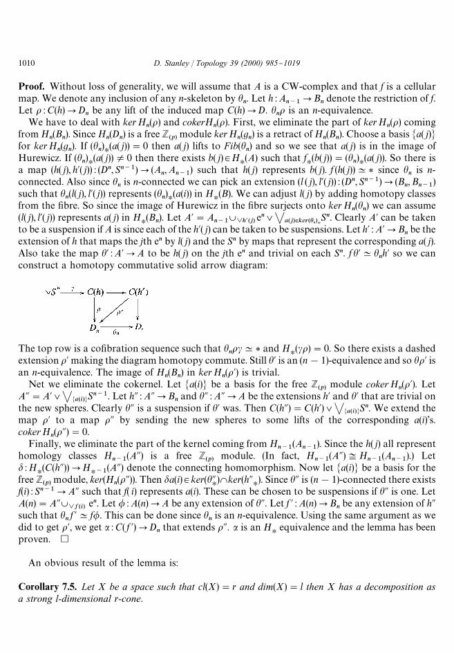
nh@ so we can

construct a homotopy commutative solid arrow diagram:

The top row is a co"bration sequence such that hnocK* and H

H(co)"0. So there exists a dashed

extension o@ making the diagram homotopy commute. Still h@ is an (n!1)-equivalence and so ho@ isan n-equivalence. The image of H

n(B

n) in kerH

n(o@) is trivial.

Net we eliminate the cokernel. Let Ma(i)N be a basis for the free Z(p)

module coker Hn(o@). Let

AA"A@sSMa(i)NSn~1. Let hA : AAPB

nand hA : AAPA be the extensions h@ and h@ that are trivial on

the new spheres. Clearly hA is a suspension if h@ was. Then C(hA)"C(h@)sSMa(i)NSn. We extend the

map o@ to a map oA by sending the new spheres to some lifts of the corresponding a(i)'s.coker H

n(oA)"0.

Finally, we eliminate the part of the kernel coming from Hn~1

(An~1

). Since the h( j) all representhomology classes H

n~1(AA) is a free Z

(p)module. (In fact, H

n~1(AA) +H

n~1(A

n~1).) Let

d : HH(C(hA))PH

H~1(AA) denote the connecting homomorphism. Now let Ma(i)N be a basis for the

free Z(p)

module, ker(Hn(oA)). Then da(i)3ker(hA

H)Wker(hA

H). Since hA is (n!1)-connected there exists

f(i) :Sn~1PAA such that f( i) represents a(i). These can be chosen to be suspensions if hA is one. LetA(n)"AAX

'f(i)en. Let / : A(n)PA be any extension of hA. Let f @ : A(n)PB

nbe any extension of hA

such that hnf @Kf/. This can be done since h

nis an n-equivalence. Using the same argument as we

did to get o@, we get a : C( f @)PDnthat extends oA. a is an H

Hequivalence and the lemma has been

proven. h

An obvious result of the lemma is:

Corollary 7.5. Let X be a space such that cl(X)"r and dim(X)"l then X has a decomposition asa strong l-dimensional r-cone.


For our purposes we need to further restrict the cone decomposition of our particular space.

Lemma 7.6. Let M>@(i)N be an r-cone decomposition of Q]Sn. Then there exists an r-cone decomposi-tion M>(i)N of Q]Sn such that H

H(>(i))"0 if *'s#n!2 and i(r. In particular this implies that

M>(i)N is an (s#n!2)-dimensional (r!1)-cone over Q]Sn.

Proof. Q]Sn is given its standard CW-decomposition (see Section 2). From Lemma 7.3 we mayassume that for every i, >@(i) is simply connected. Using Lemma 7.4 we see that >(i)

s`n~2is an

r-cone decomposition for (Q]Sn)s`n~2

. We also get a co"bration sequence:

;@(s#n) fP >@(r!1)

s`ng

P Q]Sn. (*)

Let b3Hs`n

(Q]Sn) be a generator. We look at two cases.Case (1): >@(r!1)

s`nPQ]Sn is an H

s`nsurjection. Then there is a map (h, h@) :

(Ds`n,Ss`n~1)P(>@s`n

,>@s`n~1

) such that h represents a3Hs`n

(>@) and gH(a)"b. h@ is trivial

on HH

and so by Lemma 7.2 factors through h : Ss`n~1P>@s`n~2

. Then in fact

;(s#n!2)sSs`n~1f{`h&" >@(r!1)

s`n~2PQ]Sn

is a co"bration sequence.Case (2): >@(r!1)

s`nPQ]Sn is not an H

s`nsurjection. Let d :H

H(Q]Sn)PH

H~1(;(s#n))

denote the connecting homomorphism. Then there exists (h, h@) : (Ds`n~1,Ss`n~2)P(;(s#n)

s`n~1,;(s#n)

s`n~2) such that db is represented by h. By Lemma 7.2 h@ factors through

;s`n~3

and therefore by Lemma 7.4 through a map l : Ss`n~2P;(s#n!2) such thatH

s`n~2(l)"0. Up to homotopy there exists a unique map ;(s#n!2)P;(s#n) compatible

with the maps;(i)P; of Lemma 7.4. Let k :;(s#n!2)P;(s#n) be an extension of that mapsuch that the image of the es`n~1 cell represents db.

We have a co"bration sequence:

;(s#n!2) f{P >@(r!1)

s`n~2P(Q]Sn)

s`n~2.

Also let h :>@(r!1)s`n~2

P>@(r!1) denote the inclusion. f @l is trivial on Hs`n~2

and hf @lK*therefore f @lK*. Let / :;(s#n!2)X

les`n~1P>@(r!1)

s`n~2be an extension of f @ so that we

have a homotopy commutative diagram:

We can do this using Lemma 7.2 since the map ;(s#n!2)Xles`n~1P>(r!1) is trivial on

Hs`n~1

. So there is a map o :C(/)PQ]Sn which extends the inclusion (Q]Sn)s`n~2

PQ]Sn.


Also we get a commutative diagram:

By diagram chasing we see that o must be an HH

equivalence and so a homotopy equivalence. Itfollows from what we have just shown together with Lemma 7.4 that we can take >(i)">@(i)

s`n~2if i(r and >(r)"Q]Sn. h

In the next lemma we put together what we have done to prepare for the next and "nal lemma ofthe section.

Lemma 7.7. Assume that l*n#2 and cl(Q]Sn))r. Then there exists a suspension ;Xes`n~1 anda space >. dim(;))s#n!2 and dim(>))s#n!2. Also there exists a coxbration sequence;Xes`n~1P>PQ]Sn and a map f :>PX(r!1)]Sn such that

commutes up to homotopy.

Proof. The lemma follows from Lemmas 7.6, 7.1 and 5.4. h

The next lemma is the result of this section that will be used in the next section. It singles out thetop cell of Q. This cell must already appear at the (r!1)th stage. Also we get information about itsattaching map by mapping "rst into our (r!1)-cone receiver and then projecting o! into Srl~1. Itis the interplay between this attaching map and the attaching map of the top cell that allows us to"nd the sought after obstruction.

Lemma 7.8. Assume that l*n#2 and 2p'n#2. Let g :;Xes`n~1P> be any map such thatQ]SnKC(g). Assume that dim(;))s#n!2 and that dim(>))s#n!2. Let f :>PX(r!1)]Sn be any map such that

commutes up to homotopy. Then there exists a coxbration sequence:

;@sSs`n~1P(¹r(Sl)]Sns;@)Xc esPQ]Sn (*)


such that dim(;@))s#n!2 and con(;@)*lr!2. There also exists a map / :;@PSrl~1 such that

the composition ¹r(Sl)]Sns;@project&" ;@ (P Srl~1 takes c to a unit times b.

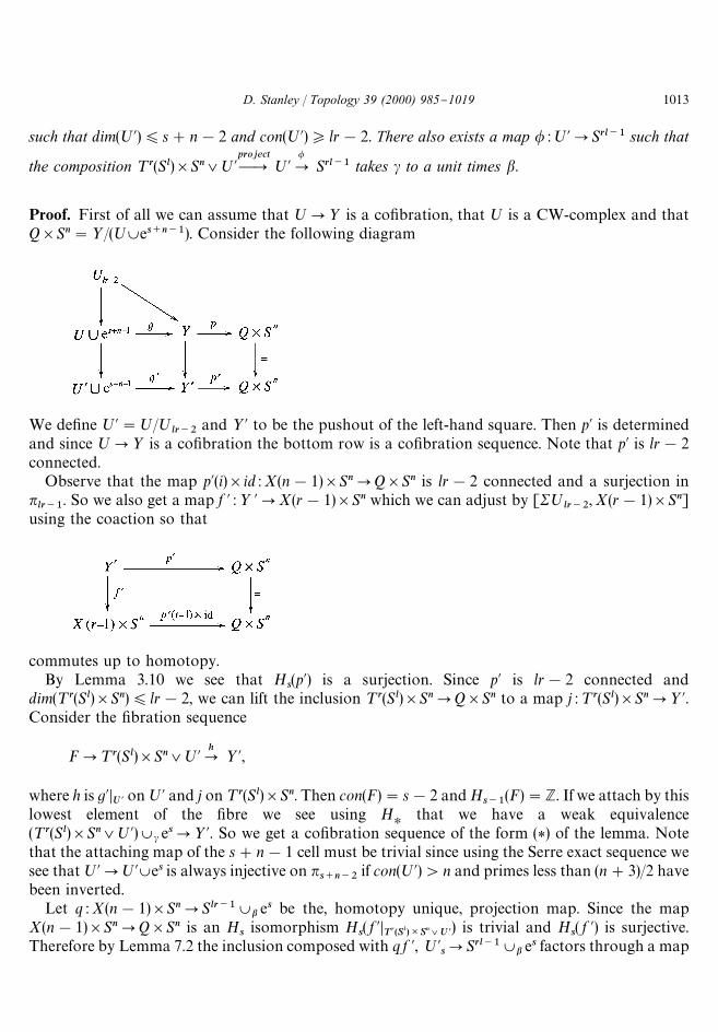
Proof. First of all we can assume that ;P> is a co"bration, that ; is a CW-complex and thatQ]Sn">/(;Xes`n~1). Consider the following diagram

We de"ne ;@";/;lr~2

and >@ to be the pushout of the left-hand square. Then p@ is determinedand since ;P> is a co"bration the bottom row is a co"bration sequence. Note that p@ is lr!2connected.

Observe that the map p@(i)]id : X(n!1)]SnPQ]Sn is lr!2 connected and a surjection innlr~1

. So we also get a map f @ :> @PX(r!1)]Sn which we can adjust by [R;lr~2

, X(r!1)]Sn]using the coaction so that

commutes up to homotopy.By Lemma 3.10 we see that H

s(p@) is a surjection. Since p@ is lr!2 connected and

dim(¹r(Sl)]Sn))lr!2, we can lift the inclusion ¹r(Sl)]SnPQ]Sn to a map j :¹r(Sl)]SnP>@.Consider the "bration sequence

FP¹r(Sl)]Sns;@ hP >@,

where h is g@DU{

on;@ and j on ¹r(Sl)]Sn. Then con(F)"s!2 and Hs~1

(F)"Z. If we attach by thislowest element of the "bre we see using H

Hthat we have a weak equivalence

(¹r(Sl)]Sns;@)Xc esP>@. So we get a co"bration sequence of the form (*) of the lemma. Notethat the attaching map of the s#n!1 cell must be trivial since using the Serre exact sequence wesee that;@P;@Xes is always injective on n

s`n~2if con(;@)'n and primes less than (n#3)/2 have

been inverted.Let q : X(n!1)]SnPSlr~1Xb es be the, homotopy unique, projection map. Since the map

X(n!1)]SnPQ]Sn is an Hs

isomorphism Hs( f @D

Tr(Sl)CS

n[U{

) is trivial and Hs( f @) is surjective.

Therefore by Lemma 7.2 the inclusion composed with q f @, ;@sPSrl~1Xb es factors through a map


/ :;@sPSrl~1. con(Srl~1)'n and 2p'n!2 so Srl~1PSrl~1Xbes is a n

iinjection for

s)i(s#n!2 and a nisurjection for s(i)s#n!2. Therefore we can extend our factoriz-

ation of the inclusion composed with gf @ to a map /@ :;@PSrl~1. Quotienting out ¹r(Sl)]Sn inboth >@ and X(n!1)]Sn we see that f @ induces a homotopy commutative diagram

such that the map on the bottom is an Hs

surjection. The second part of the lemma followseasily. h

8. Looking at loops

The goal of this section is to "nd obstructions to the existence of the co"bration sequencesproduced in the last section (Lemma 7.8). The method is to look at the implications of sucha co"bration sequence using Adams}Hilton models. We describe the Hurewicz image of theadjoint of the attaching map of the top cell of Q]Sn (Lemma 8.1). We then describe the image in anassociated space (Lemma 8.2). On the other hand, Lemma 8.4 says that certain elements cannot bein the image of Hurewicz. Again we work at a prime p. We let Q, l and b be as in the last section.Assume b is a coH map.

For a simply connected CW-complex X we let AH(X) denote the Adams}Hilton model ofX with Z

(p)coe$cients [1]. For a cellular map of CW-complexes f : XP> let f

H: AH(X)PAH(>)

denote an induced map. (The map is only determined up to homotopy.)The properties of AH(X) relevant for our purposes follow. AH(X) is a di!erential graded algebra

of the form ¹(<), the tensor algebra on <. There is a weak equivalence of di!erential gradedalgebras AH(X)PCs

H(XX) (recall Cs

Hdenotes singular chains) which is compatible up to homotopy

with cellular maps between CW-complexes. < is a free Z(p)

module with one basis element ofdimension n for every (n#1)-cell of X. If f : SnPX

nis the attaching map of an (n#1)-cell in X then

the di!erential of the corresponding basis element a has the property that d(a)"z where z is theimage in AH(X) of some lift of f a

H(nn~1

)3HH(XX

n) to the chains and then to AH(X

n). (n

n~1denotes

the generator of Hn~1

(Sn~1).) If > is a subcomplex of X then we can assume that AH(>) isa subalgebra of AH(X).

Lemma 8.1. Let

;sSs`n~1 fP ((¹r(Sl)]Sn)s;)Xc es

gP Q]Sn

be a coxbration sequence. Assume that dim(;))s#n!2. Let; have any cell structure with no cellsof dimension 's#n!2 and let the other spaces have their canonical cell structures (see Lemma 2.1).


Let a3AH(;sSs`n~1) be the generator corresponding to Ss`n~1 and b, c3AH((¹r(Sl)]Sns;)Xc es) the generators corresponding to the Sn and the es respectively. Then there area,d3AH((¹r(Sl)]Sns;)Xc es) such that f

H(a)"u[b, c]#a#d, g

H(a)"0 in AH(Q]Sn), d is

a boundary, a and d have no linear part and u is a unit.

Proof. The fact that a and d have no linear part follows since AH(¹r(Sl)]Sns;)Xc es) has nothinglinear in dimension s#n!2 (remember dim(;))s#n!2).

Next consider the diagram

where the left-hand square is a pushout and the rows are co"bration sequences. > can beconsidered as a subcomplex of Q]Sn (Q]Sn without the top cell). We let AH(>) be the correspond-ing subalgebra of AH(Q]Sn). Then since b is coH, H

H(ba)"0. So f @

H(a)"u[h

Hb, h

Hc]#d, where

d is a boundary. But ker gH"ker h

Hand h

His surjective so the lemma follows. h

Lemma 8.2. Let us again be given a coxbration sequence as in the last lemma. Let

h : ((¹r(Sl)]Sn)s;)XcesP(SnsSlr~1)Xc{es

be the map that is the projection on ¹r(Sl)]Sn, the map / from Lemma 7.8 on ; and the canonicalextension on es where c@ is the image of c. Let f and a be as in Lemma 8.1. Let b,c and e be the generatorsin AH((SnsSlr~1)Xes) corresponding to Sn, es and Slr~1 respectively. Then (hf )

H(a)"u[b, c]#a

where a3¹(b, e) and u is a unit.

Proof. (hf )H(a)3¹(b, c, e). Since lr!1'n the lemma follows from Lemma 8.1 by looking at

dimensions. h

Lemma 8.3. Let f :SlPSr be a coH map and s*2. Then the following diagram commutes:

where the vertical maps are the universal Whitehead products.

Proof. See Ref. [29, Chapter X, Theorem 8.8]. h

The next lemma says that in some cases we cannot directly add a single cell to SnsSrl~1Xfes

such that the corresponding cohomology class will be the product in cohomology of the classes


corresponding to the es and the Sn. Lemmas 7.7, 7.8, 8.1 and 8.2 essentially told us that we have tobe able to do this if we want to have an r-cone decomposition for Q]Sn.

Lemma 8.4. Assume that Rn~1bK. *. Also assume 2p!3'n, r*2 and l*n#2. Letn : SnsSlr~1PSlr~1 be the projection. Let c@ : Ss~1PSnsSlr~1 be a map such that nc"b. Then inthe notation of Lemma 8.2, the image of [b, c]#a in H

H(X(SnsSlr~1Xc es)) is not in the image of

Hurewicz for any a3¹(b, e).

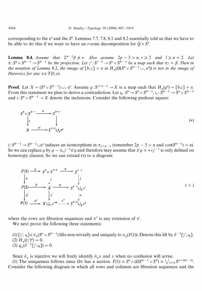
Proof. Let X"(SnsSlr~1)Xc{ es. Assume g : Ss`n~1PX is a map such that HH(ga)"[b,c]#a.

From this statement we plan to derive a contradiction. Let nb: SnPSnsSlr~1, n

e: Slr~1PSnsSlr~1

and i :SnsSlr~1PX denote the inclusions. Consider the following pushout square:

(*)

j : Slr~1PSlr~1Xes induces an isomorphism in ns`n~1

(remember 2p!3'n and con(Slr~1)'n).So we can replace g by g!in

ej~1n@g and therefore may assume that n@gK* ( j~1 is only de"ned on

homotopy classes). So we can extend (*) to a diagram:

(#)

where the rows are "bration sequences and nA is any extension of [email protected] next prove the following three statements:

(1) [c@, nb]3n

H(SnsSlr~1) lifts non-trivially and uniquely to n

H(F(1)). Denote this lift by d~1[c@, n

b].

(2) HH((c@)a)"0.

(3) qH(d~1[c@,n

b])"0.

Since dH

is injective we will freely identify dHx and x when no confusion will arrise.

(1) The uniqueness follows since Xn has a section. F(1)KSn'(XSlr~1sS0)KSiw0

Sn`i(lr~2).Consider the following diagram in which all rows and columns are "bration sequences and the


maps are the obvious ones.

In this way we see that the inclusion / : Sn`lr~2PF(1) can be taken to be [ne, nb]. Let

h : F(1)PSn`lr~2 be any map such that h/Kid. Write c@"neb#g. Since nc@"b, g lifts to n

HF(1).

Therefore hH[g, n

b]"[h

Hg, h

Hnb]"0 since h

Hnb"0. By Lemma 8.3 [b, n

b]"[n

e, nb]Rn~1b. So

hH[c@, n

b]"h

H([b, n

b]#[g, n

b])"h

H[n

e, nb]Rn~1b"Rn~1bK. *.

(2) If it were not true nothing of the form [b, c]#a would be a cycle in AH((SnsSlr~1)Xc{ es).(3) i

H[c@, n

b]"0. Since n@ is a n

s`n~1surjection (since j is one and j factors through n@) the long

exact sequence of a "bration tells us that qH(d~1[c@, n

b])"0.

Next we will show that the induced map h :Fib(i@i)PFib( j) is at least n#s!1 connected. Welook at the Z

(p)homology Serre spectral sequence EH

H,Hfor the "bration sequence

XFib(i@i)PX(SnsSlr~1)PX(XXges`n),

AH(SnsSlr~1)"¹(b, e) with the trivial di!erential and AH(XXges`n)"¹(b, c, e, f ) with

db"dc"de"0 and df"[b, c]#a (a3¹(b, e)). It is then easy to see that cokerHH(X(i@i))

is isomorphic to the image of Z(p)

Sc, cb, cb2T in dimensions less thanminMlr#s!3, 3n#s!4N*n#s (since r*2, l*n#2 and n*2). It follows that there existsc@3E2

0,s~2such that d

s~1c"c@. So there exists c@?b3E2

n~1,s~2and c@?b23E2

2n~2,s~2. Since b is

a permanent cycle and the "bration is a loop map ds~1

(cb)"c@?b and ds~1

(cb2)"c@?b2. Thenext lowest total degree in which an element of the EH

H,Hcan have a non-trivial di!erential is

minMlr#s!4,3n#s!5N*n#s!1 (in particular the elements c@?b3 or c@?e). It follows thatHH(XFib(i@i)"Z

(p)) if *"0 or s!2 and 0 if *(n#s!2 and *O0 or s!2. Therefore h is at

least n#s!1 connected.So too con(q@q)*n#s!1. But this is a contradiction since d~1[c,n

b]3kern

n`s~2(q). h

If we consider the Serre exact sequence to give a "rst-order approximation to the homology ofa "bre then in the last lemma we were required to calculate part of the second order approximation.Presumably this procedure could be formalized.

9. Existence of maps with the required properties

In our "nal section we quote some results of Brayton Gray (Theorem 9.1). They show that thereexist unstable elements in the homotopy groups of spheres with the properties we desire. We alsostate and prove our main theorem. Again we "x a prime p'2 and let Q and l be as in Sections 4,7 and 8.


Theorem 9.1 (Gray [16]). Let t,k be positive integers. Write t"plm such that (m, p)"1. Lets"t!k. If s'l then there exists X

k,s3n

t(2(p~1))`2k~1(S2k`1) such that:

(1) R2l`1Xk,sK* and

(2) R2lXk,sK. *

For our purposes we only need the following corollary of the theorem.

Corollary 9.2. Let l,r and n be any integers. Then there exists s and b3ns~1

(Slr~1) such that:

(1) b is a suspension(2) R2n~1bK. * if lr is odd and R2nbK. * if lr is even.(3) R2nbK* if lr is odd and R2n`1bK* if lr is even.

Our main theorem follows immediately.

Theorem 9.3. For every pair of positive integers t, r such that r'1 and 2t#1(2p!3 there existp-local spaces Q such that cat(Q]Sn)"catQ"r for n*2t#1, cl(Q]Sn)"clQ"r for n'2t#1and cl(Q]S2t`1)"r#1.

Proof. We merely have to choose l*2t#3 so that we have an (r!1)-cone receiver in highenough dimensions. The conclusions of the theorem then follow from Lemmas 7.7, 7.8, 8.1, 8.2, 8.4,Theorems 4.3, 4.1 and Corollary 9.2.

Corollary 9.2 gives us our elements to construct our spaces Q. Theorems 4.1 and 4.3 then showthat cat(Q]Sn)"catQ"r for n*2t#1 and cl(Q]Sn)"clQ"r for n'2t#1. So alsocl(Q]S2t`1))r#1. Lemmas 8.4 shows a certain element is not in the image of Hurewicz.However Lemmas 7.7, 7.8, 8.1 and 8.2 used in succession show that if cl(Q]S2t`1)"r then thesame element must be in the image of Hurewicz. This contradiction show thatcl(Q]S2t`1)"r#1. h

Taking more care throughout the paper (in particular giving slightly more general results inSection 6) it is possible to show that for every t'0 there also exist Q such thatcl(Q]S2t)"cat(Q]S2t)#1. This is left as an exercise for the reader.

10. Two questions

We conclude with two questions. An a$rmative answer to the "rst question would provea conjecture of Iwase [18].

Question 1. Assume that cl(X)"cat(X)"cat(X]Sn). Does this imply that cl(X)"cl(X]Sn`1)?

Question 2. Assume that cat(X]Sn)"cat(X)#1 and that cat(X)"cl(X). Does this implycl(X]Sn`1)"cl(X)#1?


Acknowledgements

I would like to thank Hans Scheerer for suggesting that I try to compute the cone length ofIwase's example and Manfred Stelzer for bringing the paper of Brayton Gray to my attention. I feelindebted to Paul Selick for introducing me to the ideas of single loop space decompositions.I would also like to thank Pascal Lambrechts and the University of Artois for inviting me asa visitor. It was during my stay there that my interest in LS category was kindled and many of thetechniques used in this paper were learnt. I again thank Pascal Lambrechts for supplying me withinexpensive housing during my stay.

References

[1] J.F. Adams, P.J. Hilton, On the chain algebra of a loop space, Comment. Math. Helv. 30 (1955) 305}330.[2] D. Anick, Non commutative algebras and their Hilbert series, J. Algebra 78 (1982) 120}140.[3] H.J. Baues, Iterierte Join-Konstructionen, Math. Zeit. 131 (1973) 77}84.[4] I. Berstein, P.J. Hilton, Category and Generalized Hopf Invariants, Illinois J. Math. 4 (1960) 437}451.[5] O. Cornea, Strong LS category equals cone-length, Topology 34 (1995) 377}381.[6] O. Cornea, Lusternik}Schnirelmann-categorical sections, Ann. Scient. ED c. Norm. Sup. 28 (1995) 689}704.[7] N. Dupont, A counterexample to the Lemaire}Sigrist conjecture, Topology 38 (1999) 189}196.[8] G. Dula, H.J. Marcum, Hopf invariants of the Berstein}Hilton}Ganea kind, Topology Appl. 65 (1995) 179}203.[9] S. Eilenberg, J.C. Moore, Homology and "brations, I. Comm. Math. Helv. 40 (1966) 199}236.

[10] Y. Felix, S. Halperin, J.-C. Thomas, Adams' Cobar equivalence, Trans. Amer. Math. Soc. 329 (2) (1992) 531}549.[11] R.H. Fox, On the Lusternik}Schnirelmann Category, Ann. Math. 42 (1941) 333}370.[12] R.H. Fox, Topological invariants of the Lusternik}Schnirelmann type, Lectures in Topology, The University of

Michigan conference of 1940, The University of Michigan Press, Michigan, 1941, pp. 293}295.[13] T. Ganea, A generalization of the homology and homotopy suspension, Comm. Math. Helv. 39 (1965) 295}322.[14] T. Ganea, Lusternik}Schnirelmann category and strong category, Illinois J. Math. 11 (1967) 417}427.[15] W.J. Gilbert, Some examples for weak category and conilpotency, Illinois J. Math. 12 (1968) 421}432.[16] B. Gray, Untable families related to the image of J, Math. Proc. Camb. Philos. Soc. 96 (1984) 95}113.[17] S. Halperin, J.-M. Lemaire, Suites inertes dans les algebres de Lie gradueH es, Math. Scand. 61 (1987) 39}67.[18] N. Iwase, Ganea's conjecture on Lusternik}Schnirelmann category, Bull. London Math. Soc. 30 (1998) 623}634.[19] N. Iwase, A

=method in Lusternik}Schnirelmann category, preprint.

[20] L. Lusternick, L. Schnirelmann, MeH thodes Topologiques dans les Problemes Variationnels, Herman, Paris, 1934.[21] M. Mather, Pull-backs in Homotopy Theory, Can. J. Math. 28 (1976) 225}263.[22] J. Milnor, On spaces having the homotopy type of a CW-complexes, Trans. Amer. Math. Soc. 90 (1959) 272}280.[23] G.J. Porter, The homotopy groups of wedges of suspensions, Amer. J. Math. 88 (1966) 655}663.[24] V. Puppe, A remark on homotopy "brations, Manuscr. Math. 12 (1974) 113}120.[25] H. Scheerer, D. TanreH , Fibrations a la Ganea, Bull. Belg. Math. Soc. 4 (1997) 333}353.[26] D. Stanley, On the Lusternik}Schnirelmann category of maps, submitted.[27] F. Takens, The Lusternick}Schnirelmann Categories of a Product Space, Compositio Math. 22 (1970) 175}180.[28] L. Vandembroucq, Ph.D. Thesis, University of Lille, 1998.[29] G.W. Whitehead, Elements of Homotopy Theory, Springer, Berlin, 1978.


Spaces with Lusternik–Schnirelmann category n and cone length n+1

Documents

Transcript of Spaces with Lusternik–Schnirelmann category n and cone length n+1