Space-time processes

NRCSE

Separability

Separable covariance structure:

Cov(Z(x,t),Z(y,s))=CS(x,y)CT(s,t)

Nonseparable alternatives

•Temporally varying spatial covariances

•Fourier approach

•Completely monotone functions

SARMAP revisited

Spatial correlation structure depends on hour of the day:

Bruno’s seasonal nonseparability

Nonseparability generated by seasonally changing spatial term

Z1 large-scale feature

Z2 separable field of local features

(Bruno, 2004)

€

Y(t,x) = μ(t,x)+ σ t (x)(α xZ1(t)+ Z2 (t,x))+ ε(t,x)

€

σt (x )

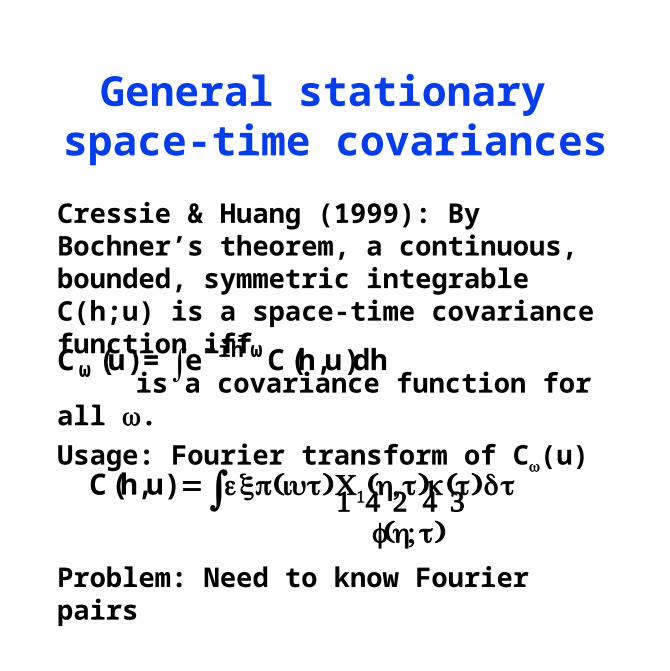
General stationary space-time covariances

Cressie & Huang (1999): By Bochner’s theorem, a continuous, bounded, symmetric integrable C(h;u) is a space-time covariance function iff

is a covariance function for all .

Usage: Fourier transform of C(u)

Problem: Need to know Fourier pairs

€

Cω(u) = e−ihTω∫ C(h,u)dh

C(h,u) = exp(iuτ)C1(h, τ)κ(τ)

f(h; τ)1 24 34 dτ∫

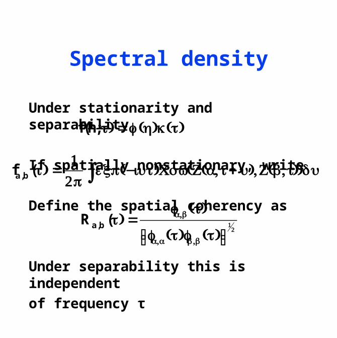
Spectral density

Under stationarity and separability,

If spatially nonstationary, write

Define the spatial coherency as

Under separability this is independent

of frequency τ

f(h;τ) =ϕ (h)κ(τ)

fa,b (τ) =12π

exp(−iuτ)Cov(Z(a, t+u),Z(b, t))du∫

Ra,b (τ) =fa,b (τ)

fa,a (τ)fb,b (τ)⎡⎣ ⎤⎦12

Estimation

Let

where R is estimated using

φa,b (τ) = tanh−1(Ra,b (τ))

fa,b (τ) = gρ (a−s)gρ (b−s)Ia+s ,b+s∗ (τ)ds

R2∫

Models-3 output

ANOVA results

Item df rss P-value

Between points

1 0.129 0.68

Between freqs

5 11.14 0.0008

Residual 5 0.346

Coherence plot

a3,b3 a6,b6

A class of Matérn-type nonseparable covariances

=1: separable

=0: time is space (at a different rate)

f(,τ) =γ(α2β2 +β2 2 + α2τ2 + 2 τ2 )−ν

scale spatialdecay

temporaldecay

space-timeinteraction

Chesapeake Bay wind field forecast (July 31, 2002)

Fuentes model

Prior equal weight on =0 and =1.

Posterior: mass (essentially) 0 for =0 for regions 1, 2, 3, 5; mass 1 for region 4.

Z(s, t) = K (s −s i, t−ti )Zi (s, t)i=1

5

∑

Another approach

Gneiting (2001): A function f is completely monotone if (-1)nf(n)≥0 for all n. Bernstein’s theorem shows that

for some non-decreasing F. In particular, is a spatial covariance function for all dimensions iff f is completely monotone.The idea is now to combine a completely monotone function and a function with completey monotone derivative into a space-time covariance

€

f(t) = e−rtdF(r)0

∞∫

€

f( h 2)

€

C(h,u) =σ2

ψ(u 2)d/ 2ϕ

h 2

ψ(u 2 )

⎛

⎝ ⎜

⎞

⎠ ⎟

€

ϕ

Some examples

€

ϕ (t) = exp(−ctγ ), c > 0,0 < γ ≤ 1

ϕ(t) =cνtν/ 2

2ν−1Γ(ν)Kν (ct1/ 2 ), c > 0,ν > 0

ϕ(t) = (1+ ctγ )− ν , c,ν > 0,0 < γ ≤ 1

ψ(t) = (atα + 1)β , a > 0,0 < α ≤ 1,0 ≤ β ≤ 1

ψ(t) =ln(atα + b)

ln(b), a > 0,b > 1,0 < α ≤ 1

A particular case

α=1/2,γ=1/2 α=1/2,γ=1

α=1,γ=1/2 α=1,γ=1

€

C(h,u) = (u 2α + 1)−1exp −h 2

(u 2α + 1)γ

⎛

⎝ ⎜

⎞

⎠ ⎟

Issues to be developed

•NonstationarityDeformation approach: 3-d spline fit;penalty for roughness in time and space

•AntisymmetryGneiting’s approach has

C(h,u)=C(-h,u)=C(h,-u)=C(-h,-u)Unrealistic when covariance caused by meteorology

•CovariatesNeed to take explicit account of covariates driving the covariance

•Multivariate fieldsMardia & Goodall (1992) use Kronecker product structure (like separability)

Temporally changing spatial deformations

where

(θ, f) a wijk Cijk −C(fk (xi ), fk (xj ); θ)( )i,j,k∑

2

+λkJ (fk ) + ηK (f)

K(f) = (fk (x) −∫k∑ fk−1(x))2dx

Velocity-driven space-time covariances

CS covariance of purely spatial field

V (random) velocity of field

Space-time covariance

Frozen field model: P(V=v)=1 (e.g. prevailing wind)

C(h,u) =EVCS (h−Vu)

C(h,−u) =C0 (h+ vu) ≠C0 (h−vu) =C(h,u)

Taylor’s hypothesis

C(0,u) = C(vu,0) for some v

Relates spatial to temporal covariance

Examples:

Frozen field model

Separable modelsC(h,u) =C0 ((a

2 h2 +b2u2 )

12 )

Irish wind data

Daily average wind speed at 11 stations, 1961-70, transformed to “velocity measures”

Spatial: exponential with nugget

Temporal:

Space-time: mixture of Gneiting model and frozen field

CT (u) =(1+ a u2α )−1

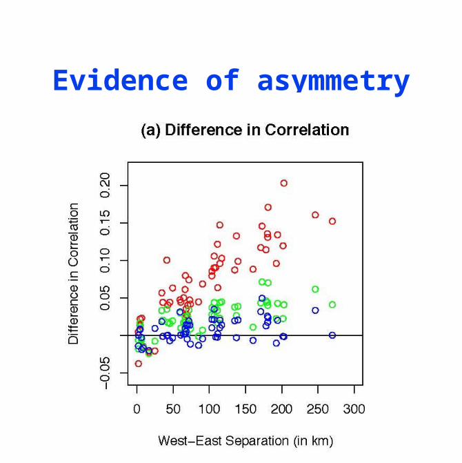
Evidence of asymmetry

Time lag 0Time lag 1Time lag 2Time lag 3