SPACE-TIME ADAPTIVE PROCESSING (STAP) - … · 4.0 SPACE-TIME ADAPTIVE PROCESSING (STAP) 4.1...

© 2014 M. C. Budge - [email protected] 1

4.0 SPACE-TIME ADAPTIVE PROCESSING (STAP)

4.1 Introduction

We now want to briefly discuss space-time adaptive processing, or STAP. When we discuss radars we normally consider the processes of beam forming, matched filtering and Doppler processing separately. By doing this we are forcing the radar to operate on only one domain at a time: space for beam forming, fast time for matched filtering and slow time for Doppler processing. At some time in the 1970’s or 1980’s radar analysts noted that this separation of functions may be sacrificing capabilities because the processor was not making use of all available information, or degrees of freedom. Suppose we have a linear phased array that has N elements. In terms of beam forming to maximize the target return and minimize returns from interference (e.g., clutter

and jammers) we say that we have N degrees of freedom. Suppose that in a Doppler processor we process M pulses. In this case we say that we have M degrees of freedom with which to maximize the signal return and minimize interference (e.g., clutter, jamming and noise). In our normal methods whereby we separate beam forming and Doppler processing we have a total of M+N degrees of freedom. Now, if we were to consider that we could perform Doppler processing at each antenna element and then form the beam we would have MN degrees of freedom.

Figure 1 might help in visualizing this further. It contains a depiction of angle-Doppler space. Each of the squares corresponds to a particular angle and Doppler. There are N beam positions and M Doppler cells. The dark square indicates an angle and Doppler that contains clutter. With our standard processing techniques we could null the clutter by suppressing a beam position and by suppressing a Doppler cell. We would do these independently. The suppressed beam position is denoted by the crosshatched cells and the suppressed Doppler is denoted by the dotted cells. It will be noted that in the process of suppressing the clutter cell we suppress other cells. This happens because we separately process in angle and Doppler space. With STAP we would, ideally, simultaneously process in both angle and Doppler space and suppress only the cell containing the clutter.


4.2 Spatial Processing

To begin talking about STAP techniques we need to establish the math that seems to be used when discussing STAP. With STAP, the processor design technique involves maximizing the ratio of signal power to interference plus noise power (SINR) at the output of the processor. The maximization technique is based on the Cauchy-Schwarz inequality, the same method we used in matched filter theory.

4.2.1 Signal Only

To start the problem we consider the antenna problem first. In particular, we consider a linear array of N elements as shown in Figure 2. In

that figure, it is assumed that the target is located at an angle of s relative to

boresight. From linear array theory we can write the output of the linear array as

1

2 sin

0

s

Nj kd

s k s

k

V w P e

. (1)

If we define

0

1

1N

w

w

w

w (2)

Figure 1 – Clutter Nulling Using Conventional Techniques


and

0

2 sin

1

2 1 sin1

1

s

s

j d

s

j N dN

s

es

s e

s (3)

we can write sV as

H

s s sV P w s (4)

where the superscript H denotes Hermetian, or conjugate-transpose, of the

vector.

In STAP, we say that we would like to choose w so as to maximize

2

sV subject to the constraint that the norm of w remain finite. In equation

form we want to solve the problem

Figure 2 – Linear Phased Array


2 22

2

max max max

subject to constant

H H

s s s s sV P P

w w w

w s w s

w

. (5)

To solve this problem we invoke one of the Cauchy-Schwarz inequalities.

Specifically, if w and ss are column vectors then

2 22H

s s w s w s (6)

with equality when

s w s (7)

where is an arbitrary constant. If we apply this to our problem with 1 we

get the familiar antenna solution of

2 sin

2 1 sin

1

s

s

j d

j N d

e

e

w (8)

or

2 sin

2 1 sin

1

s

s

j d

j N d

e

e

w . (9)

We note that if we replace ss with s , allow to vary from 2 to 2

and compute

22 HV w s (10)

we get the radiation pattern of the linear array. This pattern will have a peak at

s and a sin sinNx x shape.

4.2.2 Noise Only

To extend this idea to adaptive processing we next want to consider the case where the input to each antenna element is only noise. This is illustrated in Figure 3. Following the pattern from above, we can write the noise voltage at the output of the summer as

1

0

NH

N k k

k

V w n

w n (11)


where

0

1

1N

n

n

n

n . (12)

Since the noise is a random variable, we can write the noise power at the output of the summer as1

22 H H H H

no N nP E V E E R w n w nn w w w . (12)

In the above nR is termed the interference (receiver noise only in this case)

covariance matrix.

4.2.3 Signal and Noise – SNR

With this we can write the SNR at the output of the summer as

2

H

s sso

H

no n

PPSNR

P R

w s

w w. (13)

If we assume that n is zero-mean and uncorrelated across the elements of the

array we can write

1 Implied in the above is that there is a receiver attached to each element of the array and that

the summing of the outputs of the elements is performed in the signal processor. Thus, the array is an active array that contains T/R modules. This configuration is taken for granted in radars that might employ STAP.

Figure 3 – Array with only noise


2

n N NR I P I (14)

and

2

2

H

s s

N

PSNR

P

w s

w. (15)

If we recognize 2

w as a scalar constant that we force to be non-zero and finite,

we can again invoke the Cauchy-Schwarz inequality to maximize SNR by

maximizing 2

H

sw s . Doing this leads to the same solution as given above in

Equation (7).

We point out that the above development is analogous to the derivation

of the matched filter in waveform theory. It also leads to the same result. That is, the “filter” that maximizes SNR is matched to the signal.

4.2.4 Correlated Interference – SINR

We now consider the case where the interference is correlated across the array. This interference could be clutter or jammers. The appropriate model we

need to work with is given in Figure 4. In this figure, Inn represents the

interference “voltage” and is a zero-mean, random variable. The subscript n is used to represent the nth interference source (which we will need shortly when we consider multiple interference sources). The fact that the same random variable is applied to each of the antenna elements makes the outputs of the

elements random variables that are correlated. Thus, we can write In nV as

1

2 sin

0

n

Nj kd H

In n k In In

k

V w n e

w n (16)

where

In In nn n d (17)

and

2 sin

2 1 sin

1

n

n

j d

n

j N d

e

e

d . (18)

nd is termed the steering vector for the nth interference source.


We allow for multiple interference sources by simply summing the voltages for the multiple sources. Specifically, we write.

1

K

I In n

n

n

n d . (19)

We further assume that the interference sources are independent so that

0

In

In Ik

P n kE n n

n k

. (20)

We write the interference power (from the K interference sources) as

2

H H H H

I I I I IP E E R w n w n n w w w . (21)

In the above we write IR as

1 1 1

K K KH H

I I I In Il n l In n

n l n

R E E n n P D

n n d d (22)

where we have made use of Equation (20) and

Figure 4 – Array with Interference


2 sin

2 1 sin2 sin

2 1 sin

1

1n

nn

n

H

n n n

j d

j N dj d

j N d

D

ee e

e

d d

. (23)

If we combine Equation (12) with Equation (21), we get the total interference power as

H H

n I no I n IP P P R R R w w w w . (24)

With the above, the signal-to-interference-plus-noise ratio (SINR) at the output of the summer is given by

2

H

s sso

H

n I

PPSINR

P R

w s

w w. (25)

The objective of the STAP algorithm is to maximize the SINR. To do this via the Cauchy-Schwarz inequality we need to manipulate Equation (25). We start by noting that, because of the receiver noise, R will be positive definite. This

means that 1 2R is real and that

1 2R exists, and is also real. We can use this

to write

2 2

1 2 1 2

2

H H

s s s R R s

H

R

P R R PSINR

R

w s w s

w w w (26)

This is of the same form as Equation (15). With this we can state that the SINR is maximized when

R R s w s . (27)

If we let 1 and substitute for Rw and R ss we get the solution

1

sR w s . (28)

The net effect of the above equation is that the antenna weights, w , are

selected to place the main beam on the target and simultaneously attempt to place nulls at the angular locations of the interference sources. We will demonstrate this through an example. Before doing so, we note that a critical

part of this development is the fact that the interference consists of both receiver noise and other interference sources such as clutter or jammers. The fact that we have included receiver noise is what makes the R matrix positive

definite, and more importantly, non-singular. Without this, 1R would not exist

and we would need to use another approach for finding the weights, w . One of

the common approaches is to use a mean-squared criterion such as least-mean-squared estimation or pseudo inverse. Both of these approaches are beyond the scope of this course.


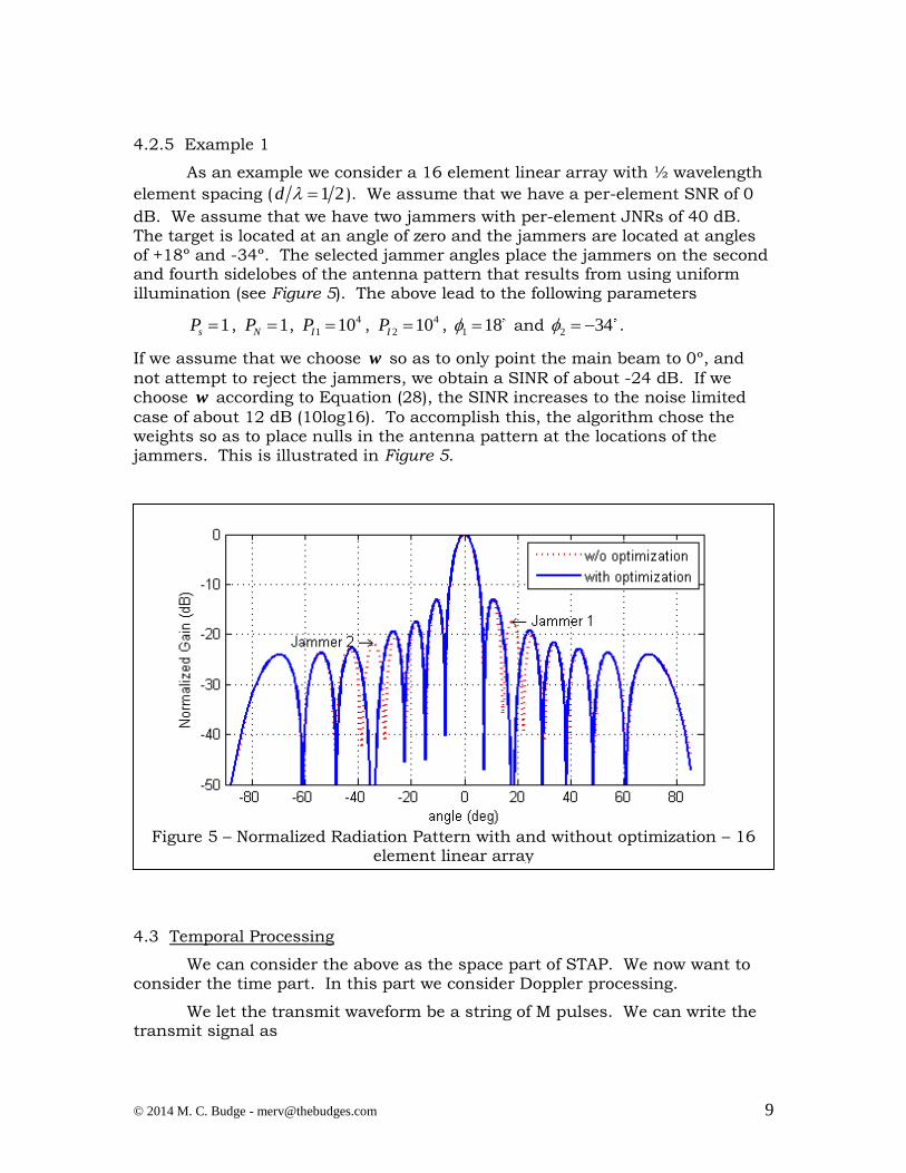
4.2.5 Example 1

As an example we consider a 16 element linear array with ½ wavelength

element spacing ( 1 2d ). We assume that we have a per-element SNR of 0

dB. We assume that we have two jammers with per-element JNRs of 40 dB. The target is located at an angle of zero and the jammers are located at angles of +18º and -34º. The selected jammer angles place the jammers on the second and fourth sidelobes of the antenna pattern that results from using uniform illumination (see Figure 5). The above lead to the following parameters

1sP , 1NP , 4

1 10IP , 4

2 10IP , 1 18 and 2 34 .

If we assume that we choose w so as to only point the main beam to 0º, and

not attempt to reject the jammers, we obtain a SINR of about -24 dB. If we

choose w according to Equation (28), the SINR increases to the noise limited

case of about 12 dB (10log16). To accomplish this, the algorithm chose the weights so as to place nulls in the antenna pattern at the locations of the jammers. This is illustrated in Figure 5.

4.3 Temporal Processing

We can consider the above as the space part of STAP. We now want to consider the time part. In this part we consider Doppler processing.

We let the transmit waveform be a string of M pulses. We can write the transmit signal as

Figure 5 – Normalized Radiation Pattern with and without optimization – 16

element linear array


1

2

0

c

Mj f t

T

l

v t e p t lT

(29)

where we have used p t as the general form of a pulse. If the pulse were a

simple unmodulated pulse we would have

rectp

tp t

. (30)

For an LFM pulse we would have

2

rectj t

p

tp t e

. (31)

The exponential term in Equation (29) represents the carrier part of the transmit signal.

The return signal, from a point target, is a delayed version of Tv t . That is

1

2 2

0

2 2c

Mj f t R t c

R T

l

v t v t R t c e p t R t c lT

. (32)

If the target is moving at a constant range-rate we can write R t as

0R t R Rt . (33)

From earlier radar courses we recall that we can write a good approximation of

Rv t as

0

12 2 2

0

c d

Mj R j f t j f t

R R

l

v t e e e p t lT

. (34)

In Equation (34), 2df R and 02R R c . From our experience with

waveforms, we recognize that we can further approximate Rv t as2

0

12 2 2

0

c d

Mj R j f t j f lT

R R

l

v t e e e p t lT

(35)

In the receiver we heterodyne to remove the carrier and normalize away the first complex constant. We also match filter the signal. The result is

1

2

0

d

Mj f lT

M R

l

v t e m t lT

(36)

where m t is the response of the matched filter to p t .

2 The approximation is based on the assumption that the phase shift caused by the Doppler doesn’t change across a compressed pulse width.


For the next step we sample Mv t at times RCt lT . That is, we

sample the return from each transmitted pulse in some range cell, RC . The

result is a sequence of samples that we denote as

20, 1dj f lT

l d RCV f e m l M

. (37)

where RCm is the (generally complex) value of Rm t lT evaluated at

RCt lT . If we sample Rm t lT at it’s peak we will use RC Sm P for a

target (desired signal) and RC Inm n for an interference signal. Inn is a zero

mean, random variable with a variance of InP . In subsequent work we will

assume that we sample at the peak of Rm t lT .

We assume that the Doppler processor is an M length finite impulse

response (FIR) filter. As such, we can write its output as

1 1

2

0 0

d

M Mj f lT

d l l d RC l

l l

V f V f m e

. (38)

It will be noted that Equation (38) is of the same for we used in the spatial processing problem. Given this we can write the signal voltage as

1

2

0

d

Mj f lT H

s S l S s

l

V f P e P f

s . (39)

Similarly, we can write the interference voltage3 as

1

2

0

n

Mj f lT H H

In n In l In n In

l

V f n e n f

d n . (40)

In Equations (39) and (40) the vectors sfs and nfd are Doppler “steering”

vectors for the signal and interference, respectively. Finally, we write the receiver noise at the FIR output as

1

0

MH

N l l

l

V n

n (41)

where the ln are zero-mean, independent, random variables with a variance of

NP .

Since Equations (39), (40) and (41) are the same form as those used in the spatial processing problem we can use the same techniques for finding the that maximizes SNR or SINR.

3 Note: to be meaningful in Doppler processing we restrict the interference to coherent types of signals, i.e.

clutter. If we have a broadband noise jammer we would treat it as receiver noise for the temporal

processing part of STAP.


4.4 Adaptivity Issues

With the above we have discussed both the space and time parts of STAP. However, we haven’t really addressed the adaptive part. In concert with the above methodologies for characterizing the target angle and Doppler, and the angles and Dopplers of the interference sources, the adaptive part would involve re-specifying the target steering vector and the R matrices on each dwell (sequence of M pulses). Since we are changing these on each dwell we compute new sets of weights on each dwell. Thus, we are changing the antenna (space) and Doppler (time) processing so that it adapts to our interpretation of the target and interference environment.

4.5 Space-Time Processing

We now want to address the issue of combined space and time processing. In a classical sense, this would be considered true space-time processing. In space-time processing, rather than form a function of angle or a function of Doppler, we combine spatial and temporal equations for the signal (Equation (1) and Equation (39)) to form a combined function of angle and Doppler. In equation form we write

1 12 sin 2

0 0

1 12 sin 2

0 0

, s s

s s

N Mj kd j lf T

s s s k l

k l

N Mj kd j lf T

s k l

k l

V f P w e e

P w e e

. (42)

We recognize the above as a sum of MN terms. If we generalize the product of the weights to MN distinct weights we get

1 1

2 sin 2

,

0 0

, s s

N Mj kd j lf T

s s s k l

k l

V f P w e e

. (43)

If we organize the weights into a general weight vector, w , and the 2 sin 2j kd j lfTe e

terms into a generalized steering vector, s , we can write

,s sV f in the same form we used above. Specifically,

, ,H

s s s sV f f w s . (44)

Further, if we extend the interference representation from earlier we can write the interference as

H

N I n IV w n (45)

where

1

,K

n I n I n Iq n n

n

n f

n n n n d . (46)


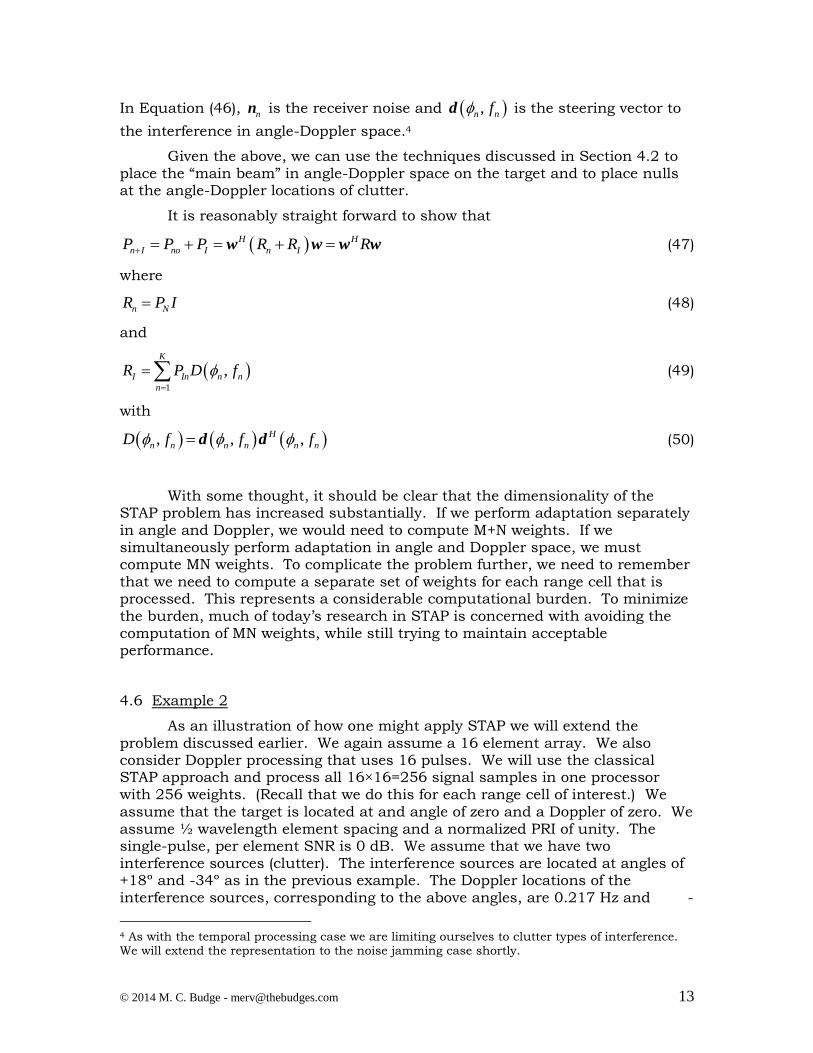
In Equation (46), nn is the receiver noise and ,n nfd is the steering vector to

the interference in angle-Doppler space.4

Given the above, we can use the techniques discussed in Section 4.2 to place the “main beam” in angle-Doppler space on the target and to place nulls at the angle-Doppler locations of clutter.

It is reasonably straight forward to show that

H H

n I no I n IP P P R R R w w w w (47)

where

n NR P I (48)

and

1

,K

I In n n

n

R P D f

(49)

with

, , ,H

n n n n n nD f f f d d (50)

With some thought, it should be clear that the dimensionality of the STAP problem has increased substantially. If we perform adaptation separately in angle and Doppler, we would need to compute M+N weights. If we simultaneously perform adaptation in angle and Doppler space, we must compute MN weights. To complicate the problem further, we need to remember that we need to compute a separate set of weights for each range cell that is processed. This represents a considerable computational burden. To minimize the burden, much of today’s research in STAP is concerned with avoiding the computation of MN weights, while still trying to maintain acceptable performance.

4.6 Example 2

As an illustration of how one might apply STAP we will extend the problem discussed earlier. We again assume a 16 element array. We also consider Doppler processing that uses 16 pulses. We will use the classical STAP approach and process all 16×16=256 signal samples in one processor with 256 weights. (Recall that we do this for each range cell of interest.) We

assume that the target is located at and angle of zero and a Doppler of zero. We assume ½ wavelength element spacing and a normalized PRI of unity. The single-pulse, per element SNR is 0 dB. We assume that we have two interference sources (clutter). The interference sources are located at angles of +18º and -34º as in the previous example. The Doppler locations of the interference sources, corresponding to the above angles, are 0.217 Hz and -

4 As with the temporal processing case we are limiting ourselves to clutter types of interference. We will extend the representation to the noise jamming case shortly.


0.28 Hz respectively. The SCRs of the two clutter sources is 50 dB. With this we get the following parameters

1sP , 1NP , 5

1 10IP , 5

2 10IP , 1 18 , 2 34 , 1 0.217 Hzf and

2 0.28 Hzf .

We write

2 sin

2 12

2 1 sin

,

1

1n

nn

n

T

n n n n

j d

j M f Tj f T

j N d

f f

ee e

e

D d d

. (51)

and form the column vector ,n nfd by concatenating the columns of ,n nfD

which is an N by M matrix. The ,s sfs vector is a column of 256 ones, which

puts the target at an angle of zero and a Doppler frequency of zero. We next use the equations of Section 4.2 to find the 256 element weight vector, w . The

weight vector is formed into a two-dimensional weight matrix, W by reversing

the algorithm used to form ,n nfd from ,n nfD . Finally, we can find the

angle-Doppler image analogous to Figure 5 by using a two-dimensional, inverse FFT with the weight matrix as the signal. The results of the above process are shown in Figures 6 and 7. Figure 6 is the angle-Doppler plot for the case where there is no interference. Figure 7 is the angle-Doppler plot for the case described above. The presence of the two nulls is clearly visible on Figure 7 as is the main beam at (0,0). The numbers beside the color bar to the right of the figures denote relative amplitudes in dB. Note the difference in the scales between Figure 6 and Figure 7. This difference indicates that the null depth in Figure 7 is quite large.


Figure 6 – Angle-Doppler Map Without Optimization

Figure 7 – Angle-Doppler Map With Optimization


In the above examples, the SINR before optimization was -13.4 dB. After optimization the SINR was 24.1 dB, the noise limited value (i.e. 10log(256)).

As an interesting experiment, the optimization was extended to include two desired targets: one at (0,0) and another at (ang,Doppler)=(34º,-0.217 Hz). Figure 8 contains the angle-Doppler map for the case of the two targets and only receiver noise. It will be noted that the optimization placed peaks at the locations of the two targets. Figure 9 corresponds to the case where the two interference sources were included. It will be noted that the peaks at the locations of the targets is still present. Also, upon careful examination, and comparison to Figure 7, it will be noted that the two nulls are also present. In this case, the SINR on each target before optimization was -13.4 dB, as with the previous case. The SINR after optimization was 21.1 dB. This is not as high as

for the single-target case but is still very good.

In the above work, we assumed that we knew the locations and strengths of the interference sources. In practice this may not be the case. If it isn’t one must form the interference covariance matrix, R , by sampling the environment. Discussions of this can be found in texts on STAP.

Figure 8 – Angle-Doppler Map Without Optimizatin – Two Targets


4.7 STAP With a Noise Jammer

To handle a noise type of jammer with space-time processing we need to

modify the definition of ,n nfD in Equation (51). This type of interference will

be correlated in angle but not across the pulses. Therefore, we will have a

spatial component to the steering matrix, ,n nfD , but the temporal

component will consist of independent random variables. To model this we write the steering matrix as

2 sin

1 2 1

2 1 sin

,

1

J

J

T

J J J J

j d

J J J M

j N d

n

en n n

e

D d n

. (52)

where the Jkn are be zero-mean, independent, random variables with a variance

of JP .

The resulting ,J Jnd would look like

Figure 9 – Angle-Doppler Map With Optimization – Two Targets


1

2

2

,

J J

J J

n J

J nJ

n

nn

n

d

dd

d

(53)

which is vector of length MN. The resulting covariance matrix would be

0 0

0

0 0

J

J

J J

J

D

DR P

D

(54)

where JD is defined in Equation (23). We note that to properly form

,J Jnd we concatenate columns of ,n nfD and ,J JnD . The weights that

are computed for a jammer will place a null at J that spans across all

frequencies.

4.8 Adaptivity Again

Thus far we have discussed the space and time parts of STAP. We now want to revisit issues related to adaptivity.

In our work so far we assumed that we knew the various parameters needed to compute the optimum weights. In particular, we had enough

information to compute the R matrix. In some applications this is not the case

and we must estimate R through measurements. A potential procedure for doing this follows.

For each antenna element (T/R module) and pulse we sample the combined noise and interference in range cells we believe contains the

interference but not the target.5. We then use the samples to estimate R . Specifically, if we write the combined noise and interference voltage on a

particular sample as l

n IV we can form an estimate of R as

1

1ˆL

Hl l

n I n I

l

R V VL

(55)

where L is the number of samples taken. As a point of clarification it should

be noted that l

n IV is an MN element vector.

A question that arises is: how large does L need to be. If 1L we will be

multiplying an MN element vector by its Hermetian to produce an MN by MN

matrix. This matrix will have a rank of 1 since it has only one independent

5 In practice we can allow the range cells to contain the target return is the overall SNR and SIR is very small for each antenna element/pulse.


column. This means that R̂ has only one non-zero eigenvalue. Thus R̂ is

singular and 1R̂ doesn’t exist. This means that solving for w by the previous

method will not work.

Given that l

n IV consists of a bunch of random numbers there is a chance

that R̂ will have a rank equal to the number of samples that are taken

(assuming L MN ). Thus, to have any chance of obtaining a R̂ that is non-

singular, at least MN samples of l

n IV must be taken. As L becomes larger it

provides a better and better approximation of R 6.

Guerci has an equation that relates L to the SINR improvement. Specifically, he denotes as the SINR improvement actually obtained versus

the theoretical SINR improvement. He writes

2

1

L MNL MN

L

. (56)

Thus, for L MN we get

2 2

1 1

MN MN

MN MN

. (57)

For the case of Example 2 we have 256MN . Thus the expected SINR based

on 256 samples of l

n IV will be 2/257 or about 21 dB below the optimum SINR

improvement. If we increase L to 2MN or 512 samples we would get

2 2 1

2 1 2

MN MN

MN

. (58)

Thus, the expected SINR improvement based on R̂ would be about 3 dB below the optimum SINR improvement. However, we note that this represents a large number of samples that will require extensive time and radar resources.

4.9 Practical Considerations

If practice we may be able to get by with using fewer samples of if we have a reasonable estimate of the receiver noise power, and the interference power is large relative to the receiver noise power. We would use the

aforementioned approximation to form and estimate of IR , the interference

covariance matrix. If we term this estimate ˆIR we would form R̂ from

ˆ ˆI NR R P I (59)

where NP is the receiver noise power estimate (per antenna element and pulse).

6 Gureci, J. R., Space-Time Adaptive Processing for Radar, Artech House, 2003, ISBN 1-58053-377-9.


This approach is termed diagonal loading. Adding the term NP I assures that R̂

will be positive definite and that 1R̂ exists.

With this method the number of samples, L , needed is chosen to be at least as large as the number of anticipated interference sources. As should be

obvious, this will generally be much smaller than MN .

This method can have problems in that sometimes the eigenvalues of R̂

become ill behaved. This, in turn, causes R̂ to become ill conditioned, and the optimization to put nulls in the wrong locations. To get around this problem

one needs to take more samples and/or increase NP . The problem with taking

more samples is obvious in that it requires an extra expenditure of time and

radar resources. Increasing NP increases will cause the SIR, and SINR,

improvement to degrade, potentially to unacceptable levels.

More information about these and other practical aspects of STAP can be found in Guerci’s book and other sources.

SPACE-TIME ADAPTIVE PROCESSING (STAP) - … · 4.0 SPACE-TIME ADAPTIVE PROCESSING (STAP) 4.1...

Documents

Transcript of SPACE-TIME ADAPTIVE PROCESSING (STAP) - … · 4.0 SPACE-TIME ADAPTIVE PROCESSING (STAP) 4.1...