SPACE IN A HETEROGENEOUS MONETARY UNION: NORMAL TIMES … · 2020-01-24 · SPACE IN A...
51
DEBT SUSTAINABILITY AND FISCAL SPACE IN A HETEROGENEOUS MONETARY UNION: NORMAL TIMES VS THE ZERO LOWER BOUND 2020 Javier Andrés, Pablo Burriel and Wenyi Shen Documentos de Trabajo N.º 2001
Transcript of SPACE IN A HETEROGENEOUS MONETARY UNION: NORMAL TIMES … · 2020-01-24 · SPACE IN A...

DEBT SUSTAINABILITY AND FISCAL
SPACE IN A HETEROGENEOUS
MONETARY UNION: NORMAL TIMES
VS THE ZERO LOWER BOUND
2020
Javier Andrés, Pablo Burriel and Wenyi Shen
Documentos de Trabajo
N.º 2001

DEBT SUSTAINABILITY AND FISCAL SPACE IN A HETEROGENEOUS
MONETARY UNION: NORMAL TIMES VS THE ZERO LOWER BOUND

Documentos de Trabajo. N.º 2001
2020
(*) We thank Dennis Bonam, seminar participants at the Banco de España, the 21st Bank of Italy Workshop on Public Finance, the Fiscal Policy Seminar 2018 at the Federal Ministry of Finance in Berlin, the 2019 Computing in Economics and Finance Conference and an anonimous referee for their comments and suggestions. Javier Andrés acknowledges the financial support by the Spanish Ministry of Economy and Competitiveness (grant ECO2017-84632-R) and Generalitat Valenciana (Conselleria d’Educació, Investigació, Cultura i Esports, grant GVPROMETEO2016-097).(**) Andrés: Departamento de Análisis Económico, Universidad de Valencia, Valencia, Spain, [email protected]. (***) Burriel: Fiscal Policy Unit, DG Economics and Statistics, Banco de España, Madrid, Spain, [email protected]. (****) Shen: Department of Economics, Oklahoma State University, Stillwater, OK 74078, [email protected].
Javier Andrés (**)
UNIVERSIDAD DE VALENCIA
Pablo Burriel (***)
BANCO DE ESPAÑA
Wenyi Shen (****)
OKLAHOMA STATE UNIVERSITY
DEBT SUSTAINABILITY AND FISCAL SPACE
IN A HETEROGENEOUS MONETARY UNION:
NORMAL TIMES VS THE ZERO LOWER BOUND (*)

The Working Paper Series seeks to disseminate original research in economics and fi nance. All papers have been anonymously refereed. By publishing these papers, the Banco de España aims to contribute to economic analysis and, in particular, to knowledge of the Spanish economy and its international environment.
The opinions and analyses in the Working Paper Series are the responsibility of the authors and, therefore, do not necessarily coincide with those of the Banco de España or the Eurosystem.
The Banco de España disseminates its main reports and most of its publications via the Internet at the following website: http://www.bde.es.
Reproduction for educational and non-commercial purposes is permitted provided that the source is acknowledged.
© BANCO DE ESPAÑA, Madrid, 2020
ISSN: 1579-8666 (on line)
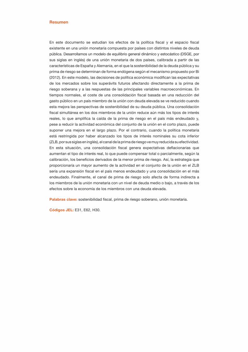
Abstract
In this paper we study fi scal policy effects and fi scal space for countries in a monetary union
with different levels of public debt. We develop a dynamic stochastic general equilibrium
(DSGE) model of a two-country monetary union, calibrated to match the characteristics
of Spain and Germany, in which debt sustainability is endogenously determined a la Bi
(2012) to shape the responses of the risk premium on public debt. Policy shocks change
the market’s expectation about future primary surplus, producing a direct effect on the
sovereign risk premium and macroeconomic responses of the economy. In normal times
the costs of a government spending driven fi scal consolidation in the high-debt country are
greatly diminished when this consolidation improves endogenously its debt sustainability
prospects. Fiscal consolidations in both members of the monetary union decrease
real interest rates and amplify the reduction in risk premium in the highly-indebted country,
improving union-wide output in the long run, but at the cost of lower output in the low-
debt country in the short term. On the contrary, when monetary policy is constrained at the
zero lower bound, the risk premium channel arising from the endogenous determination
of debt sustainability becomes muted. In the ZLB, a fi scal consolidation generates
defl ation expectations which increase the real interest rate and may compensate partially
or completely, depending on the calibration, the benefi ts from a lower risk premium. In
this context, a fi scal expansion in the low-debt country and a consolidation in the high-
debt country delivers the greater positive impact on union-wide output. Finally, the risk
premium channel only affects countries with medium or low levels of public debt indirectly
through the negative spillovers from other high-debt members of the monetary union.
Keywords: fi scal sustainability, sovereign debt default risk, monetary union.
JEL classifi cation: E31, E62, H30.
Resumen
En este documento se estudian los efectos de la política fi scal y el espacio fi scal
existente en una unión monetaria compuesta por países con distintos niveles de deuda
pública. Desarrollamos un modelo de equilibrio general dinámico y estocástico (DSGE, por
sus siglas en inglés) de una unión monetaria de dos países, calibrada a partir de las
características de España y Alemania, en el que la sostenibilidad de la deuda pública y su
prima de riesgo se determinan de forma endógena según el mecanismo propuesto por Bi
(2012). En este modelo, las decisiones de política económica modifi can las expectativas
de los mercados sobre los superávits futuros afectando directamente a la prima de
riesgo soberana y a las respuestas de las principales variables macroeconómicas. En
tiempos normales, el coste de una consolidación fi scal basada en una reducción del
gasto público en un país miembro de la unión con deuda elevada se ve reducido cuando
esta mejora las perspectivas de sostenibilidad de su deuda pública. Una consolidación
fi scal simultánea en los dos miembros de la unión reduce aún más los tipos de interés
reales, lo que amplifi ca la caída de la prima de riesgo en el país más endeudado y,
pese a reducir la actividad económica del conjunto de la unión en el corto plazo, puede
suponer una mejora en el largo plazo. Por el contrario, cuando la política monetaria
está restringida por haber alcanzado los tipos de interés nominales su cota inferior
(ZLB, por sus siglas en inglés), el canal de la prima de riesgo ve muy reducida su efectividad.
En esta situación, una consolidación fi scal genera expectativas defl acionarias que
aumentan el tipo de interés real, lo que puede compensar total o parcialmente, según la
calibración, los benefi cios derivados de la menor prima de riesgo. Así, la estrategia que
proporcionaría un mayor aumento de la actividad en el conjunto de la unión en el ZLB
sería una expansión fi scal en el país menos endeudado y una consolidación en el más
endeudado. Finalmente, el canal de prima de riesgo solo afecta de forma indirecta a
los miembros de la unión monetaria con un nivel de deuda medio o bajo, a través de los
efectos sobre la economía de los miembros con una deuda elevada.
Palabras clave: sostenibilidad fi scal, prima de riesgo soberano, unión monetaria.
Códigos JEL: E31, E62, H30.

BANCO DE ESPAÑA 7 DOCUMENTO DE TRABAJO N.º 2001
1 Introduction
The global financial and economic crisis left a legacy of historically high levels of public
debt in advanced economies, at a scale unseen during modern peace time. Keeping public
debt at high levels, however, is a source of vulnerability in itself, particularly given the
arising fiscal and economic pressures from ageing. A high public debt burden is even more
problematic in a monetary union like the euro area (EA), as monetary policy focuses on
the EA aggregate while fiscal policy decisions remain at the national level. As shown in
Figure 1, although the average debt to GDP ratio in the EA stays high at 90 percent, a
great dispersion exists across countries. In fact countries with reasonably low debt levels by
the end of 2018, standing at around or below 60 percent, including Germany (61 percent)
and The Netherlands (52 percent), coexist with others characterized by high debt levels,
around or above 100 percent of GDP, including France (98 percent), Italy (132 percent)
and Spain (97 percent). In those highly indebted countries, borrowing costs have increased
sharply, which undermine their solvency, all the more if they have to face a severe slowdown
in economic growth in the near future. Moreover, risks to debt sustainability in a high-
debt large Member State, like the ones recently experienced in Italy, can entail risks to the
stabilization of the monetary union as a whole, while cross-country spillovers of disorderly
default can threaten the very existence of the EA.
Despite the difficult financial position in some countries, the debate on fiscal strategies
is far from settled in the Euro area. The mandate to reduce public deficits and debt is
the official policy although there is some disagreement about the timing of that process.
Also the weakening of the recovery phase has stirred up some fears that unconventional
monetary stimuli might be losing steam and many voices have been raised in favor of a more
expansionary fiscal stance, at least in the core countries of the EMU in which sustainability
issues are less pressing. But also, more recently, the IMF (WEO 2019) suggested that in
case of a further weakening in growth, high-debt countries could temporarily slow down their
fiscal consolidation efforts, provided the financial markets permit this and debt sustainability
is not put at risk. Much of the support for this fiscal expansion relies on the idea that the
safe interest rate is expected to be below the nominal growth rate in the near (and even in
the distant) future, so that "public debt may have no cost" (Blanchard (2019)) However,
if the interest rate carries a risk premium and if this is affected not only by the actions
in the country with high debt but also by what other countries in the monetary union do,
the case in favor of fiscal activism ought to be revisited. If that is the case the cost of
debt might be significant and fiscal multipliers smaller, making fiscal consolidation more
appealing, depending on the prevailing monetary conditions in the union.

BANCO DE ESPAÑA 8 DOCUMENTO DE TRABAJO N.º 2001
Figure 1: Evolution of government debt and spreads in the euro area
In this paper we assess the effect of alternative fiscal policy actions in a monetary union in
which individual country members differ in the risk of sustainability of their public finances.
Countries with low and high public debt to GDP ratios coexist (where high and low will be
defined more precisely later on) and the fiscal actions can be either coordinated or unilateral
and may happen in normal monetary policy times or when the area wide monetary authority
is constrained by the lower bound of the interest rate. We pay special attention to the cross-
country spillovers of fiscal polices in this setup.
We extend a standard dynamic stochastic general equilibrium (DSGE) model of a two-
country monetary union along the lines of Benigno and Benigno (2006), modified to allow
for debt sustainability to be endogenously determined. In particular, (partial) government
default may occur, so that a haircut is applied whenever the debt of one of the country
members of the monetary union becomes unsustainable. In the model debt sustainability is
operationalized through the use of the concept of "fiscal limit" along the lines defined by
Bi (2012). In particular, the fiscal limit is the maximum amount of public debt relative to
GDP that the government can finance without defaulting on their financial commitments,
and is calculated as the expected discounted sum of maximum primary surplus that can be
generated in the future, given the current fiscal strategy and the expected evolution of the
economy. Given exogenous fluctuations in fiscal policy shocks and political risk, this fiscal
limit is stochastic. Therefore, investors may demand risk premia on government debt when
the probability of hitting the fiscal limit increases beyond some level, even if the fiscal limit
itself has not been reached. This generates a nonlinear relationship between sovereign risk
premia and the level of government debt. As the high-debt (home) country approaches its
fiscal limit, it pays a higher default risk premium on its public debt. The low-debt (foreign)
country, however, is far away from its fiscal limit and hence pays the risk free rate.
The simulated fiscal limit, which we refer as “state-dependent fiscal limit” is dynamic, and
a function of the state of both the home and foreign economies, and the political constraints

BANCO DE ESPAÑA 9 DOCUMENTO DE TRABAJO N.º 2001
on revenue collection capacity. Policy decisions affect the fiscal limit distribution and the
sovereign risk premium. The endogeneity of the fiscal limit gives rise to a powerful sov-
ereign risk premium channel and thus to cross-country spillovers (fiscal or otherwise) in the
monetary union. These spillovers are asymmetric, inducing quite different macroeconomic
responses in the country with high debt as compared with an economy operating well away
from its fiscal limit.
In this paper, a government’s default on its debt is the result of an accident, modelled
as a random draw from the fiscal limit distribution, rather than a strategic decision. The
reason for this is that a member of a monetary union like the euro area cannot strategically
default on its debt without leaving the union, since this would immediately stop the access
of its domestic banks to the union central bank’s financing with the subsequent bank run.
Instead, the most realistic situation is, as the case of Greece in the sovereign crisis illustrated,
that if a sequence of negative (random) economic or political shocks make the government’s
debt of a member unsustainable, in the sense that it is in a trajectory that will eventually
not be financiable, then it has to enter into a program and an agreement to restructure its
debt is implemented. Therefore, the role of the government in our model is limited to setting
distortionary taxes in line with the fiscal rule.
Against this backdrop, we analyze three timely fiscal issues in the European policy debate:
the long-run consolidation process a high-debt country must endure to converge back towards
more sustainable debt levels, the impact of short-run discretionary fiscal policy in countries
with strained public finances, and the effect of fiscal policy coordination between the high-
debt and low-debt countries. In the absence of lump-sum taxes, adjusting to lower levels
of public debt is always a costly and lengthy process. However, we find that under normal
monetary conditions a discretionary consolidation effort that speeds up such process in the
high-debt country, might help in moderating that cost as long as it helps to take the debt to
GDP ratio away from the risky zone (the proximity of the fiscal limit). A fiscal consolidation
today implies higher future primary surpluses, shifting the fiscal limit distribution to the
right and reducing the probability of default on impact. This effect on the risk premium is
small but persistent in time, inducing sizeable output effects. In our simulations, a 1 percent
transitory reduction in government spending reduces the risk premium on impact by 1.5
basis points (bp), reaching a maximum of 4 bp after 5 years, and it is still 2 bp lower after
10 years. The lower financing costs significantly reduce the cost of a transitory consolidation
and generate a cumulative output multiplier of -0.49 after 10 years, suggesting expansionary
fiscal consolidation, which would be consistent with the empirical findings in Giavazzi and
Pagano (1990), Alesina et al. (1998), and Alesina and Ardagna (2010). We also analyze the
spillover effects on a high debt country from the fiscal decisions of the low-debt country and
BANCO DE ESPAÑA 10 DOCUMENTO DE TRABAJO N.º 2001
fiscal policy coordination in the union. A fiscal expansion in the foreign (low-debt) country
leads to inflation, and given its large size, increases the nominal interest rate in the Euro
Area and real interest rates in both countries. The higher real rates lower demand in the
home (high-debt) country and increase the cost of servicing the debt, thus worsening its
fiscal sustainability prospects and rising the risk premium. As debt accumulates faster, high
tax rates further depress output in the home country and reduce union output in the long
run. Alternatively, a fiscal consolidation in the foreign country lowers real interest rates and
improves home country’s debt sustainability (shifts the fiscal limit to the right). Lower debt
services increase home output and lead to long run output gain in the union, at a cost of
short run output loss in the foreign country. Given these results, in normal times the best
fiscal policy coordination in the union would be a joint consolidation, but this may not be
feasible since it would contract activity in the low-debt country. Alternatively, the high-debt
country consolidates and the low-debt country remains inactive.
When monetary policy is constrained at the zero lower bound (ZLB) these results do not
hold. The real interest rate channel works against the risk premium channel arising from the
state-dependent fiscal limit, making the response in risk premium muted. On the one hand,
a discretionary fiscal consolidation at home improves future primary surplus and lowers the
default probability. On the other hand, a fiscal consolidation generates deflation expectations
that increase the real interest rate and the cost of rolling over debt, increasing the default
probability. These two effects offset each other, but under our calibration the effect of the
increase in real interest rates dominates the improvement in risk premium derived from
the reduction in government spending, making fiscal consolidation counterproductive. The
response of the fiscal limit to other fiscal measures at home or abroad is also very different
in these circumstances (as compared with that in normal monetary conditions).
Our paper is related to several studies that connect sovereign risk premia and fiscal
sustainability. Battistini et al. (2019) study fiscal and monetary policy interactions in a closed
economy with an exogenous fiscal limit. Daniel and Shiamptanis (2012) assume government
debt is constrained by an ad-hoc fiscal limit to assess fiscal crisis probabilities in the context
of a monetary union. Polito and Wickens (2015) present a model-based measure of sovereign
credit ratings for EU countries by estimating the probability that the debt to GDP ratio
will exceed a given limit or threshold at any time over a given time horizon. Uribe and Yue
(2006) and Garcia-Cicco et al. (2010) consider an exogenous risk premium by assuming that
the sovereign risk premium is monotonically increasing in the level of government debt. In
this same line, Corsetti et al. (2013) and Batini et al. (2018) propose a model where the euro
area periphery government is faced with a fiscal limit following a beta distribution calibrated
using data for Greece, which we call "exogenous fiscal limit". Our paper constructs model-

BANCO DE ESPAÑA 11 DOCUMENTO DE TRABAJO N.º 2001
consistent state-dependent fiscal limits that account for interactions among economic policy,
changes in the environment or social attitudes towards taxes, and the sovereign risk premium.
This method captures endogenous responses of fiscal limits to economic disturbances, which
strengthen significantly the risk premium channel. In particular, we show that making
the fiscal limit state-dependent reduces the government spending multiplier by 60 percent
compared with what is obtained in the model with an exogenous fiscal limit.
Our analysis is also related to papers that study cross-border spillovers from fiscal stimu-
lus, such as Corsetti et al. (2010), Arce et al. (2016), Blanchard et al. (2017) and Farhi and
Werning (2016). These works find that fiscal adjustment instruments, structural reforms,
and monetary policy all matter for the magnitude of fiscal spillovers in the Euro Area, but
they do not incorporate default risk.
Finally, our paper is not meant to add to the theory of sovereign default, as in Eaton and
Gersovitz (1981), Arellano (2008), Mendoza and Yue (2012) and Dovis (2019). These papers
model the strategic sovereign default decision of an optimizing government that accounts
for the economic costs in making default decisions. In this paper, as was mentioned above,
rather than making the default decision a strategic choice, we opt to treat the intrinsically
political decision as a random draw from the fiscal limit distribution. The reason for this
modelling choice is twofold. First, in a monetary union like the euro area a strategically
default on its debt would imply leaving the union. This very interesting research question
is related to the reasons to form a currency union, as in Chari et al. (2019), but beyond the
scope of this paper. Second, this way our model retains the DSGE framework convenient for
incorporating several economic and policy shocks and conducting fiscal experiments without
explicitly modeling the strategic default decision.
The paper is organized as follows. In the next section the baseline model is described,
while section 3 details the model calibration. Section 4 explains how the model-consistent
state-dependent fiscal limit is derived and how it is affected by macroeconomic fundamentals
and policy decisions. In section 5 the main fiscal policy experiments are described. Finally,
section 6 concludes.
2 Model
We use a two-country New Keynesian model to analyze a monetary union along the lines
of Benigno and Benigno (2006), augmented with endogenously determined state-dependent
fiscal limits and interest risk premia. Specifically, the monetary union consists of two coun-
tries, home and foreign, each inhabited by a continuum of households, with parameter s
determining the relative size of the home country. The foreign variables are defined with an

BANCO DE ESPAÑA 12 DOCUMENTO DE TRABAJO N.º 2001
asterisk. To incorporate sovereign default risk and capture different fiscal positions of union
members, our model allows for the possibility of (partial) government default in the home
country: a haircut is applied when the home country’s level of debt becomes unsustainable.
The concept of debt sustainability is operationalized by the “fiscal limit”, which will be
defined below. As debt approaches the fiscal limit, households in the home country may
demand risk premia on government debt. We assume that the public debt to GDP ratio
in the foreign country is sufficiently low so that, for simplicity, we assume there is no fiscal
limit in this country that pays always the risk free rate. In the rest of the section we will
describe the model for the home country and only mention the rest of the union when there
is an asymmetry.
2.1 Households
The home country is populated by a large number of households indexed by h ∈ [0, s), while
those living in the foreign country are indexed by f ∈ [s, 1]. Preferences are given by:
maxct,Bt,nt
Et
∞
t=0
βtc1−σt
1− σ− n1+ϕt
1 + ϕ(1)
where β is the households’ subjective discount factor, ct is consumption and nt the house-
holds’ labor supply. The inverse of intertemporal elasticity of substitution, σ, measures
relative risk aversion. The parameter ϕ governs the Frisch elasticity of labor supply. The
household receives nominal wages Wt and monopoly profits Υt from the firm, both of which
are taxed at the rate τ t. The household maximizes utility subject to the budget constraint,
Ptct +BtRt+Dt
Rft= (1− δt)Bt−1 +Dt−1 + (1− τ t)(Wtnt + PH,tΥt) (2)
where Pt is the CPI and PH,t is the PPI.
The government debt in the home country, Bt, is subject to default risk. The default
decisions depend on a realized effective fiscal limit, BHt , drawn from a fiscal limit distribution
BH(St), conditional on the state St. Specifically,
δt =
⎧⎨⎩ 0 if bt−1 < BH(St)
δ if bt−1 ≥ BH(St)(3)
where bt−1 =Bt−1Pt
is the real government debt. If the real value of debt at the beginning of
period t, bt−1, exceeds the effective fiscal limit, BHt , then the government partially defaults

BANCO DE ESPAÑA 13 DOCUMENTO DE TRABAJO N.º 2001
and outstanding debt at the beginning of period t becomes (1− δ) bt−1, otherwise it repays
in full amount with δt = 0. The derivation of BH(St) is described in Section 4.1. Governmentdebt in the home country, therefore, pays a risky yield of Rt. In addition, households may
also hold a risk-free bond, Dt, that pays the risk-free rate Rft , with an aggregate zero net
supply in each country.
where Γ0 = RER0λ0λ∗0
Rf0R0(1−δ1) = 1, is a constant including only initial conditions for asset
holdings and interest rates, which we assume equal to 1 to simplify the analysis.
+
λt = βRftEtλt+1πt+1
(6)
Optimization conditions for households in the home country are:
nϕt = λt(1− τ t)wt (4)
λt = βRtEt(1− δt+1)λt+1
πt+1(5)
λ
where λt = c−σt , πt+1 =Pt+1Pt, and wt = Wt
Ptis the real wage. The latter two equations
determine the interest rate spread on risky government debt. The households’ optimization
problem must also satisfy the following transversality condition:
limj→∞
Etβj+1λt+j+1
λt(1− δt+j+1)bt+j = 0 (7)
Since the foreign government will never default on its debt, foreign bonds (B∗t ) pay the
risk-free rate (Rft ). In this case we have the standard intertemporal Euler equation:
λ∗t = βRftEtλ∗t+1π∗t+1
(8)
where λ∗t = c∗t−σ, π∗t+1 =
P ∗t+1P ∗t. Using both Euler equations in the two countries ((6) and
(8)), we can derive an arbitrage condition linking the real exchange rate, RERt =P ∗tPt, to
differences in nominal interest rates and consumption levels
RERt = Γ0λtλ∗t
Rft−1Rt−1 (1− δt)
(9)

BANCO DE ESPAÑA 14 DOCUMENTO DE TRABAJO N.º 2001
2.2 Final consumption goods
Households consume the following basket of final goods produced at home, cH,t, and abroad,
cF,t,
ct =cH,tη
ηcF,t1− η
1−η(10)
where η represents the preference by home consumers for goods produced at home. There
exists home bias in consumption when η > 12. The demand for final goods produced at home
and abroad and the home consumer price index are
cH,t = ηPF,tPH,t
1−ηct = ηtot1−ηt ct (11)
cF,t = (1− η)PF,tPH,t
−ηct = (1− η)tot−ηt ct (12)
Pt = PηH,tP
1−ηF,t (13)
where tott = PF,t/PH,t represents the relative terms of trade.
2.3 Final intermediate goods
Differentiated Intermediate goods produced at home yH,t(h) are bundled together into final
home intermediate goods yH,t, according to the following technology:
yH,t =1
s
1θ s
0
yH,t(h)θ−1θ dh
θθ−1
(14)
where θ represents the elasticity of substitution between different good-varieties, equal across
regions, and θθ−1 is the price mark-up. These final intermediate goods can be used to produce
final home or foreign consumption goods (cH,t(h) or c∗H,t(h)) and home public spending (gt).
Cost minimization on the part of final goods producers results in the following demand curve
for the intermediate home good, yH,t(h), and the corresponding home producer price index,
PH,t,
yH,t(h) =1
s
pH,t(h)
PH,t
−θyH,t, (15)
PH,t =1
s
s
0
pH,t(h)1−θdh
11−θ. (16)

BANCO DE ESPAÑA 15 DOCUMENTO DE TRABAJO N.º 2001
1Note that we have defined the real wage in terms of the CPI (wt = WtPt), while the real marginal cost is defined in terms of
domestic PPI (mct(h) =MCt(h)PH,t
)
maxnt(h),PH,t(h)
Et
∞
t=τ
βtλtλτ
PH,t(h)
PH,tyt(h)−mctyt(h)−
ψ
2
PH,t(h)
πPH,t−1(h)− 1
2
yt (17)
subject to:
yt(h) = ant(h) =PH,t(h)
PH,t
−θyt (18)
The first order condition after imposing symmetry across firms is
(1− θ) + θmct − ψπH,tπ− 1 πH,t
π+ ψβEt
λt+1λt
πH,t+1π
− 1 πH,t+1π
yt+1yt
= 0 (19)
which represents the home non-linear New Keynesian Phillips curve (NKPC) under Rotem-
berg pricing.
2.5 Government
The government (of each country member of the union) finances unproductive purchases
(gt) by collecting tax revenue and issuing one-period bonds (Bt). The tax revenue is raised
through a distortionary time varying tax rate (τ t) on labor income. The government sets the
distortionary tax according to a tax rule and therefore, contrary to the literature on strategic
default (Eaton and Gersovitz (1981), Arellano (2008), Mendoza and Yue (2012) and Dovis
(2019)), it does not internalize the fact that it may default on its debt. It faces the following
budget constraint:
2.4 Intermediate goods production
Intermediate goods producers adopt a linear production technology, yt(h) = atnt(h), with
real marginal costs, mct(h) = PtPH,t
wtat1 and technology at, assumed constant (at = a). These
firms enjoy some monopoly power in producing a differentiated product and therefore face
a downward sloping demand curve, but are also subject to Rotemberg (1982) quadratic-
adjustment costs in changing prices. That is, in each period, firms pay a cost proportional
in real terms to aggregate real income pact (i) =ψ2
PH,t(i)
πPH,t−1(i)− 1
2
yt to be able to change
their prices and this penalizes large price changes in excess of steady state inflation rates.
The dynamic problem of firm h is:
BtRt+ τ t 1−
ψ
2
πH,tπ− 1
2
PH,tyt = (1− δt)Bt−1 + PH,tgt (20)

BANCO DE ESPAÑA 16 DOCUMENTO DE TRABAJO N.º 2001
2The fiscal rule and the fiscal limit represent different constraints to the accumulation of public debt. The former ensuresthat the fiscal level is bounded and does not enter into an explosive path. The fiscal limit simply reflects the fact that theremay be some level of debt that even when stable, it cannot be financed given the tax system and the political constraints inthe country, and that gives rise to a non zero probability of default.
Note that in the case of the home country, where default may happen, the relevant stock
of debt is the one net of default ((1− δt)Bt−1). We assume only domestic households may
purchase domestic government bonds, that is, there is total home bias on domestic debt. In
our model, default is costless in the sense that the defaulting government is neither forced
to reform its policies by dramatically reducing deficits, nor is it locked out of credit markets
for some period. The government’s budget constraint can be rewritten in real terms as
btRt+
τ t 1− ψ2
πH,tπ− 1 2
yt − gttot1−ηt
=(1− δt) bt−1
πt(21)
where bt = Bt/Pt is real government debt.
The distortionary tax is set according to a simple tax rule2
τ t = τ + γb(bt−1 − b) (22)
where γb > 0 is the tax adjustment parameter, so that a larger γb means that the government
is more willing to retire debt by raising the tax rate, making debt converge back quicker to
its long-run steady state. We assume that government purchases follow an AR(1) process
lngtg= ρg ln
gt−1g+ εgt (23)
where g is the steady state government purchase at home.
2.6 Monetary policy
The Central Bank of the Monetary Union sets the gross nominal interest rate to stabilize
union-wide inflation and follows a regime-switching process:
Rt =
⎧⎪⎪⎨⎪⎪⎩R + απ(πMU,t − πMU), if sRt = 1
1, if sRt = 2(24)
where απ is the policy response to union-wide inflation, and πMU,t = sπt + (1 − s)π∗t . In aTaylor rule regime (sRt = 1), the Central Bank obeys the Taylor principle and in a zero lower
BANCO DE ESPAÑA 17 DOCUMENTO DE TRABAJO N.º 2001
3We impose the ZLB by exogenous regime switching in monetary policy rules, similar to Richter and Throckmorton (2015),to minimize the number of state variables in solving the nonlinear model. In section 5, the responses of the real interest ratefrom fiscal shocks are qualitatively similar to the ones that would be found under endogenous ZLB events.
4This is a reasonable assumption since the import content of government spending in the largest Euro Area countries is verysmall, at around 10%.
bound regime (sRt = 2), the Central Bank exogenously pegs the gross nominal interest rate
at 1. Thus, all ZLB events are due to exogenous changes in sRt , and the switches between
the two monetary policy regimes are similar to large exogenous shocks.3
The monetary policy regime index sRt evolves according to the transition matrix⎛⎝ p1 1− p11− p2 p2
⎞⎠ .where p1(p2) is the probability of continuing to stay in the Taylor rule (ZLB) regime each
period, calibrated to be persistent.
2.7 Union-wide demand and market clearing
Union-wide demand for home goods, yDt , comes from the producers of home and foreign final
consumption goods (cH,t, c∗H,t), home government spending (assuming absolute home bias in
government spending gH,t = gt4) and to pay for price adjustment costs
yDt (h) = scH,t(h) + sgH,t(h) + (1− s)c∗H,t(h) +ψ
2
πH,tπ− 1
2
yt. (25)
Substituting the demands from (15) above we get5
yDt (h) =pH,t(h)
PH,t
−θtot1−ηt
scHMU,t + gt +
ψ
2
πH,tπ− 1
2
yt (26)
where we define union-wide private consumption of home produced goods as cHMU,t = ηct +
η∗ 1−ssc∗t .
The real exchange rate, the ratio of relative consumption price levels, can be expressed
as the ratio of the home and foreign producer prices
RERt =P ∗tPt=
PF,tPH,t
η−η∗
= totη−η∗
t (27)
5We assume the law of one price holds: (i.e.: the price of variety h(f) of the home (foreign) good is equal at home andabroad).

BANCO DE ESPAÑA 18 DOCUMENTO DE TRABAJO N.º 2001
6 See Ascari and Rossi (2012) for the equivalence of the first-order condition on the NK Phillips curve for the Rotemberg andCalvo specifications on price stickiness.
To derive the equilibrium in the goods market in the home country we equate the demand
for each intermediate good producer of the home product, equation (26), with its production
function yDt (h) = yt(h) and aggregate across all home intermediate firmss
0yt(h)dh to get
ant 1−ψ
2
πH,tπ− 1
2
= tot1−ηt cHMU,t + gt (28)
where we have defined home aggregate labor as nt =s
0nt (h) dh.
Union-wide output is defined as
yMU,t = syt + (1− s)y∗t (29)
Finally, as the representative household at Home is a pool of identical units trying to
hedge aggregate risk and we do not allow them to purchase risk-free bods from the foreign
government, there is zero net supply of home’s risk-free bonds. Hence, provided that the
Euler conditions for Home risk-free and risky bonds hold, only the latter are traded to satisfy
the government’s budget constraint. This final condition closes our economy.
3 Calibration
The model is calibrated at a quarterly frequency. In general, the home country is calibrated
using data for Spain and the foreign country using data for Germany. However, there are
a number of parameters which are common across countries. The household discount rate
is 0.99. Preference over consumption are logarithmic, so σ = 1. The inverse of the Frisch
elasticity of labor supply is set to ϕ = 1. The productivity levels at the steady state are
normalized to 1.
The price elasticity of demand, θ, is assumed to be 11, indicating a steady state markup
of 10 percent. Alvarez et al. (2006) and Vermeulen et al. (2012) find that prices in the
euro area are sticky and price durations are significantly longer than in the US. In addition,
survey results show that in the euro area about two-thirds of firms do not change their prices
more than once a year (Fabiani et al., 2005). In line with this empirical evidence, we set the
Rotemberg adjustment parameter, ψ, to 357.5, which implies that 15 percent of the firms
reoptimize prices each quarter.6

BANCO DE ESPAÑA 19 DOCUMENTO DE TRABAJO N.º 2001
The two countries are assumed to have the same degree of home bias, η = 1− η∗ = 0.63,
calibrated from Euro Area’s import share. We calibrate the size of the home country by
comparing the nominal GDP of the Euro Area periphery (Spain & Italy) vs core (Germany
& France), and s = 0.36.7 The fiscal parameters are calibrated to match Spain and German
data since the creation of the euro area (1999-2016). In steady state, government purchases
Table 1: Parameter calibration
parameters values
β 0.99 the discount factor
σ 1 inverse of the intertemporal elasticity of substitution
ϕ 1 inverse of Frisch elasticity of labor supply
θ 11 elasticity of substitution
ψ 357.5 Rotemberg adjustment parameter
η 0.63 home country bias in home goods
η∗ 0.37 foreign country bias in home goods
s 0.36 share of home country
b/y 0.6 steady state debt to output ratio (home)
b∗/b∗ 0.6 steady state debt to output ratio (foreign)
g/y 0.183 steady state gov spending to output ratio (home)
g∗/y∗ 0.187 steady state gov spending to output ratio (foreign)
τ 0.3005 steady state income tax rate (home)
τ∗ 0.3425 steady state income tax rate (foreign)
γb 0.04 tax response parameter to changes in debt
ρg, ρg∗ 0.9 AR(1) coefficient in government spending rules
σg,σg∗ 0.01 standard deviation of government spending shock
απ 1.5 Taylor rule parameter to inflation
p1 0.9917 regime-switching parameter for the normal monetary policy regime
p2 0.65 regime-switching parameter for the ZLB regime
δ 0.07 quarterly haircut on debt if default occurs
7Thus, the relative size of the domestic economy (s = 0.36) is meant to encompass a broader group of countries in the unionwith comparable debt sustainability problems, so that fiscal responses in this group of countries exert some meaningful effectson the monetary union as a whole.
are 18.3 and 18.7 percent of GDP, respectively, and the tax rates are 0.3005 and 0.3425, while
the steady state debt-to-GDP ratio is 0.6 for both countries and the model implied lump-sum
transfers are 9.5 and 13 percent of GDP. The tax adjustment parameter in the fiscal rule γb
BANCO DE ESPAÑA 20 DOCUMENTO DE TRABAJO N.º 2001
8Bi et al. (2018) show that a higher Taylor rule parameter is needed when the rule is targeting the risky rate and the haircutδ is sizable. On the contrary, this is not the case when the rule is targetting the risk-free rate like in our model.
is calibrated to 0.04. The magnitude of fiscal adjustments is kept small, just sufficient to
satisfy the transversality condition for government debt.
The shock processes for gt and g∗t are calibrated on the basis of the empirical evidence
available for the euro area and Spain and Germany. For instance, Gadatsch et al. (2015)
and Batini et al. (2018) estimate a model of a monetary union with Spain and Germany
as members and get the following parameter values for the government spending processes:
ρg = ρg∗= 0.9 and σg = σg
∗= 0.01. These numbers are in line with the theoretical literature
(see Schmitt-Grohe and Uribe (2007)).
The steady-state inflation rate is assumed to be π = 1 for simplicity. The Taylor rule
parameter is 1.5.8 For the transition probability in the regime switching process of monetary
policy, we use p1 = 0.9917, which gives an average length of a Taylor rule regime of 30 years,
and a less persistent ZLB regime is required to maintain the stationarity of the equilibrium
system. We calibrate p2 = 0.65, which implies an average length of a ZLB regime of 2.8
quarters.
Our default scheme assumes a constant haircut rate, δ. We follow Bi (2012) who uses
the estimated haircut rates of sovereign debt restructures in emerging market economies
between 1998 and 2005 from Sturzenegger and Zettelmeyer (2008), and calculates that 90
percent of the annual haircut rates (as a share of all sovereign debt) fall below 0.3. Thus, we
assume a constant annual haircut rate of 0.28, implying a quarterly rate of δ = 0.07. Table
1 summarizes the parameter values.
Appendix A lists equations that characterize the equilibrium system. We use the monotone
mapping method of Coleman (1991) and Davig (2004) to obtain a fully-nonlinear solution.
Appendix B describes the numerical solution method.
4 Fiscal limit distribution
4.1 Simulating fiscal limit distribution
Fiscal limits are defined, following Bi (2012), as the present value of maximum future pri-
mary surpluses over an infinite horizon. When the tax revenue reaches its peak, the expected
present value of future primary surpluses is maximized, given the level of government expen-
ditures. Government expenditures, monetary policy regimes, and institutional quality vary
with the stochastic shocks hitting the economy, generating a distribution for the maximum
debt level that a government is able to service.

BANCO DE ESPAÑA 21 DOCUMENTO DE TRABAJO N.º 2001
Since the fiscal limits are the maximum level of debt that can be supported without
default, when simulating fiscal limits we set δt = 0 for all t. We derive the intertemporal
government budget constraint given the real government budget constraint, (21), the Euler
equation, (6), and the transversality condition, (7),
bt−1 = πtEt
∞
j=0
βjλt+jλt
Tt+j − gt+j − ztot1−ηt+j
(30)
Following Bi et al. (2016), fiscal limits are simulated based on (30), but all the variables are
computed under τ t+i = τmax, the maximum income tax rate a government is willing and
able to impose. We set τmax = 0.435, the marginal statutory rate for highest income earners
in Spain (above 60, 000€ per year) (European Commission, 2018).9
BH(St) = βptπmax(St)Et
∞
j=0
βj1
(totmax(St+j))1−ηλmax(St+j)λmax(St)
(T max(St+j)− gt+j − z) (31)
The simulated fiscal limits are state-dependent, uncertain and conditional on an initial
state of the economy St = gt, g∗t , tott−1, s
Rt . This notion of fiscal limit also captures the
private sector’s perception of the limit, as it uses the stochastic discount factor evaluated
at the maximum tax rate, βj λmax(St+j)λmax(St) , and allows for a stochastic political risk (β
pt ) that
follows an AR(1) process,
lnβptβp= ρβ
p
lnβpt−1βp
+ εβp
t , εβp
t ∼ N(0, (σβp)2) (32)
9Another way to quantify the fiscal limit is the Laffer curve. Bi (2012) derives the peak of the Laffer curve analytically in areal business cycle model. In a nominal model, Bi et al. (2018) assume that the Central Bank is able to set the inflation rateequal to its objective, which allows for a simple solution for the main variables determining the maximum of the Laffer curve.However, in a monetary union setting the aggregate inflation at its target does not guarantee that each country’s inflation isalso equal to its target, and thus it does not allow for an analytical solution of the Laffer Curve. Trabandt and Uhlig (2011) usea model-based approach to simulate the theoretical Laffer Curve and find that for plausible calibration, the peak of the LafferCurve for Spain is 0.415.
Lower βpt indicates higher political risk and hence lower fiscal limits. A possible interpretation
for this assumption is that the policy makers have a shorter planning horizon than the private
sector (Bi et al., 2018).
In the data, risk premia in several European countries start to increase even at lower
levels of debt. Setting βp < 1 and εβp
t ∼ N(0, (σβp)2) serves to shift down the mean and
increase the dispersion of the fiscal limit, which generates plausible movements in risk premia
as observed in the data. In particular, we calibrate the political risk in the home country by
using an indicator about the current political situation derived from a Spanish nation-wide
BANCO DE ESPAÑA 22 DOCUMENTO DE TRABAJO N.º 2001
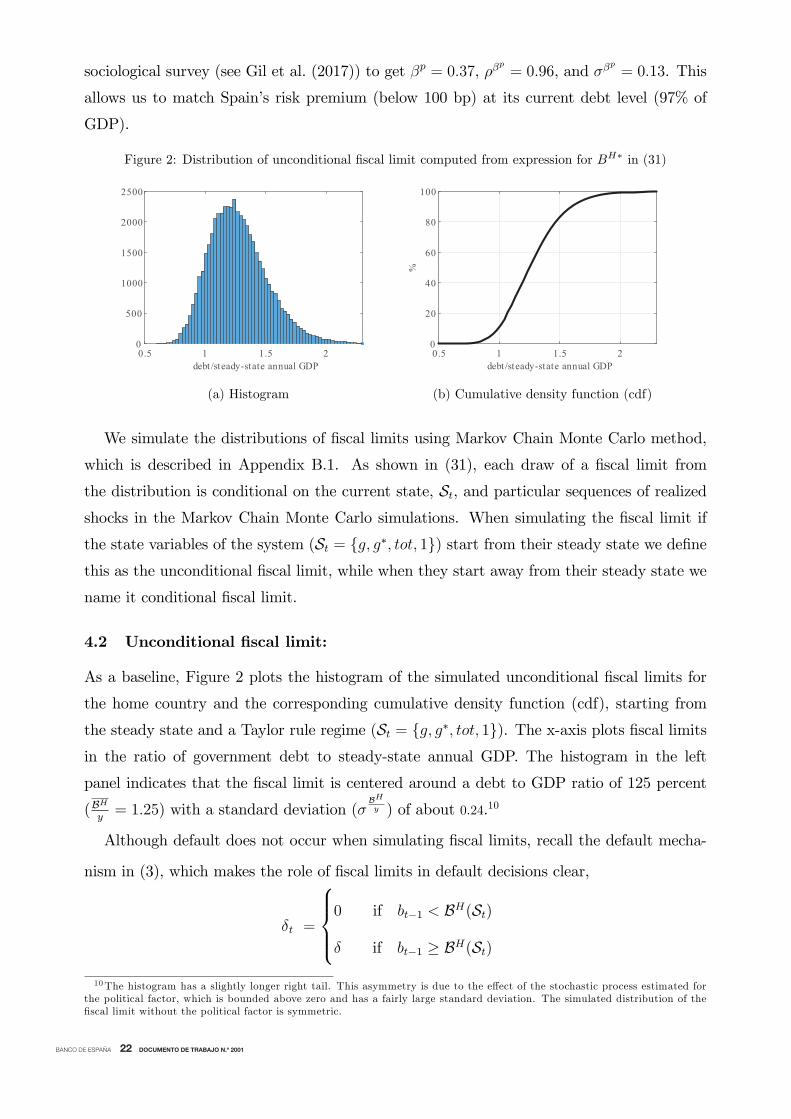
Figure 2: Distribution of unconditional fiscal limit computed from expression for BH∗ in (31)
debt /steady-state annual GDP0.5 1 1.5 20
500
1000
1500
2000
2500
debt /steady-state annual GDP0.5 1 1.5 2
%
0
20
40
60
80
100
(a) Histogram (b) Cumulative density function (cdf)
10The histogram has a slightly longer right tail. This asymmetry is due to the effect of the stochastic process estimated forthe political factor, which is bounded above zero and has a fairly large standard deviation. The simulated distribution of thefiscal limit without the political factor is symmetric.
δt =
⎧⎪⎪⎨⎪⎪⎩0 if bt−1 < BH(St)
δ if bt−1 ≥ BH(St)
sociological survey (see Gil et al. (2017)) to get βp = 0.37, ρβp= 0.96, and σβp = 0.13. This
allows us to match Spain’s risk premium (below 100 bp) at its current debt level (97% of
GDP).
We simulate the distributions of fiscal limits using Markov Chain Monte Carlo method,
which is described in Appendix B.1. As shown in (31), each draw of a fiscal limit from
the distribution is conditional on the current state, St, and particular sequences of realizedshocks in the Markov Chain Monte Carlo simulations. When simulating the fiscal limit if
the state variables of the system (St = {g, g∗, tot, 1}) start from their steady state we define
this as the unconditional fiscal limit, while when they start away from their steady state we
name it conditional fiscal limit.
4.2 Unconditional fiscal limit:
As a baseline, Figure 2 plots the histogram of the simulated unconditional fiscal limits for
the home country and the corresponding cumulative density function (cdf), starting from
the steady state and a Taylor rule regime (St = {g, g∗, tot, 1}). The x-axis plots fiscal limitsin the ratio of government debt to steady-state annual GDP. The histogram in the left
panel indicates that the fiscal limit is centered around a debt to GDP ratio of 125 percent
(BH
y= 1.25) with a standard deviation (σ
BHy ) of about 0.24.10
Although default does not occur when simulating fiscal limits, recall the default mecha-
nism in (3), which makes the role of fiscal limits in default decisions clear,
BANCO DE ESPAÑA 23 DOCUMENTO DE TRABAJO N.º 2001
The choice BH(St), is uncertain and depends on fiscal policy, monetary policy, and politicalconsiderations. The fiscal limit defined here describes the stochastic upper bound on how
much debt a government is willing and able to service given the economic and political
constraints. Therefore, there is a one to one mapping between the cumulative distribution
of the home fiscal limit and the probability of the home government defaulting on its debt.
Thus, the cumulative distribution function (cdf) of the home fiscal limit in the right panel
can be interpreted as the probability of the home government defaulting on its debt, which
is nil for debt levels close to 80 percent of GDP, while it converges to 1 for debt levels above
200 percent of GDP. In between those values, the probability of default gradually increases
as debt accumulates.
A large literature adopts strategic sovereign default approach in which an optimizing gov-
ernment accounts for some economic costs in making default decisions (Eaton and Gersovitz,
1981; Aguiar and Gropinath, 2006; Arellano, 2008; Yue, 2010; Dovis, 2019). Another litera-
ture incorporates default risk by exogenously specifying fiscal limits (Daniel and Shiampta-
nis, 2012; Corsetti et al., 2013; Batini et al., 2018). Instead, we follow a different approach.
Although the government in the model does not optimize over its default decisions, our defi-
nition of the fiscal limit captures uncertainty in default risk. Moreover, the fiscal limit, when
included in the full model, responds endogenously to economic disturbances, which we will
discuss in the next section.
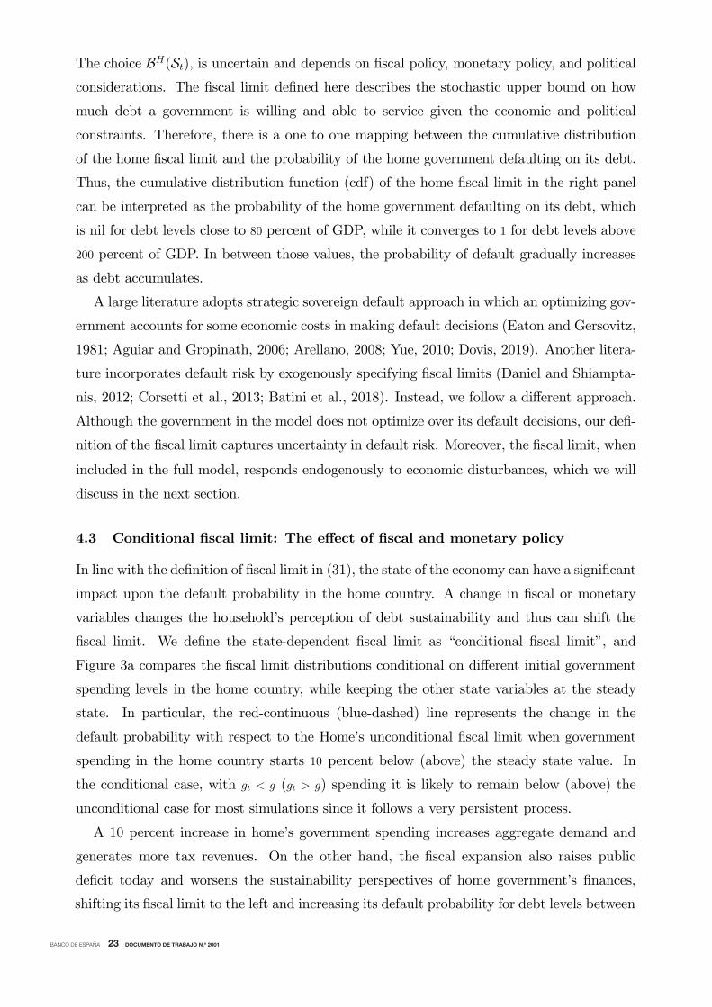
4.3 Conditional fiscal limit: The effect of fiscal and monetary policy
In line with the definition of fiscal limit in (31), the state of the economy can have a significant
impact upon the default probability in the home country. A change in fiscal or monetary
variables changes the household’s perception of debt sustainability and thus can shift the
fiscal limit. We define the state-dependent fiscal limit as “conditional fiscal limit”, and
Figure 3a compares the fiscal limit distributions conditional on different initial government
spending levels in the home country, while keeping the other state variables at the steady
state. In particular, the red-continuous (blue-dashed) line represents the change in the
default probability with respect to the Home’s unconditional fiscal limit when government
spending in the home country starts 10 percent below (above) the steady state value. In
the conditional case, with gt < g (gt > g) spending it is likely to remain below (above) the
unconditional case for most simulations since it follows a very persistent process.
A 10 percent increase in home’s government spending increases aggregate demand and
generates more tax revenues. On the other hand, the fiscal expansion also raises public
deficit today and worsens the sustainability perspectives of home government’s finances,
shifting its fiscal limit to the left and increasing its default probability for debt levels between
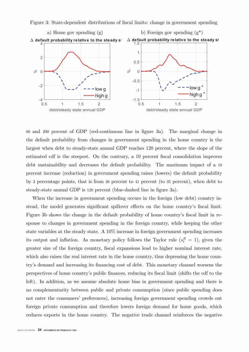
BANCO DE ESPAÑA 24 DOCUMENTO DE TRABAJO N.º 2001
Figure 3: State-dependent distributions of fiscal limits: change in government spending
a) Home gov spending (g) b) Foreign gov spending (g*)
debt/steady state annual GDP0.5 1 1.5 2
%
-4
-2
0
2
4 default probability re lative to the steady st
low ghigh g
debt/steady state annual GDP0.5 1 1.5 2
%
-1.5
-1
-0.5
0
0.5
1
1.5 default probability re lative to the steady st
low ghigh g
80 and 200 percent of GDP (red-continuous line in figure 3a). The marginal change in
the default probability from changes in government spending in the home country is the
largest when debt to steady-state annual GDP reaches 120 percent, where the slope of the
estimated cdf is the steepest. On the contrary, a 10 percent fiscal consolidation improves
debt sustainability and decreases the default probability. The maximum impact of a 10
percent increase (reduction) in government spending raises (lowers) the default probability
by 3 percentage points, that is from 38 percent to 41 percent (to 35 percent), when debt to
steady-state annual GDP is 120 percent (blue-dashed line in figure 3a).
When the increase in government spending occurs in the foreign (low debt) country in-
stead, the model generates significant spillover effects on the home country’s fiscal limit.
Figure 3b shows the change in the default probability of home country’s fiscal limit in re-
sponse to changes in government spending in the foreign country, while keeping the other
state variables at the steady state. A 10% increase in foreign government spending increases
its output and inflation. As monetary policy follows the Taylor rule (sRt = 1), given the
greater size of the foreign country, fiscal expansions lead to higher nominal interest rate,
which also raises the real interest rate in the home country, thus depressing the home coun-
try’s demand and increasing its financing cost of debt. This monetary channel worsens the
perspectives of home country’s public finances, reducing its fiscal limit (shifts the cdf to the
left). In addition, as we assume absolute home bias in government spending and there is
no complementarity between public and private consumption (since public spending does
not enter the consumers’ preferences), increasing foreign government spending crowds out
foreign private consumption and therefore lowers foreign demand for home goods, which
reduces exports in the home country. The negative trade channel reinforces the negative
BANCO DE ESPAÑA 25 DOCUMENTO DE TRABAJO N.º 2001
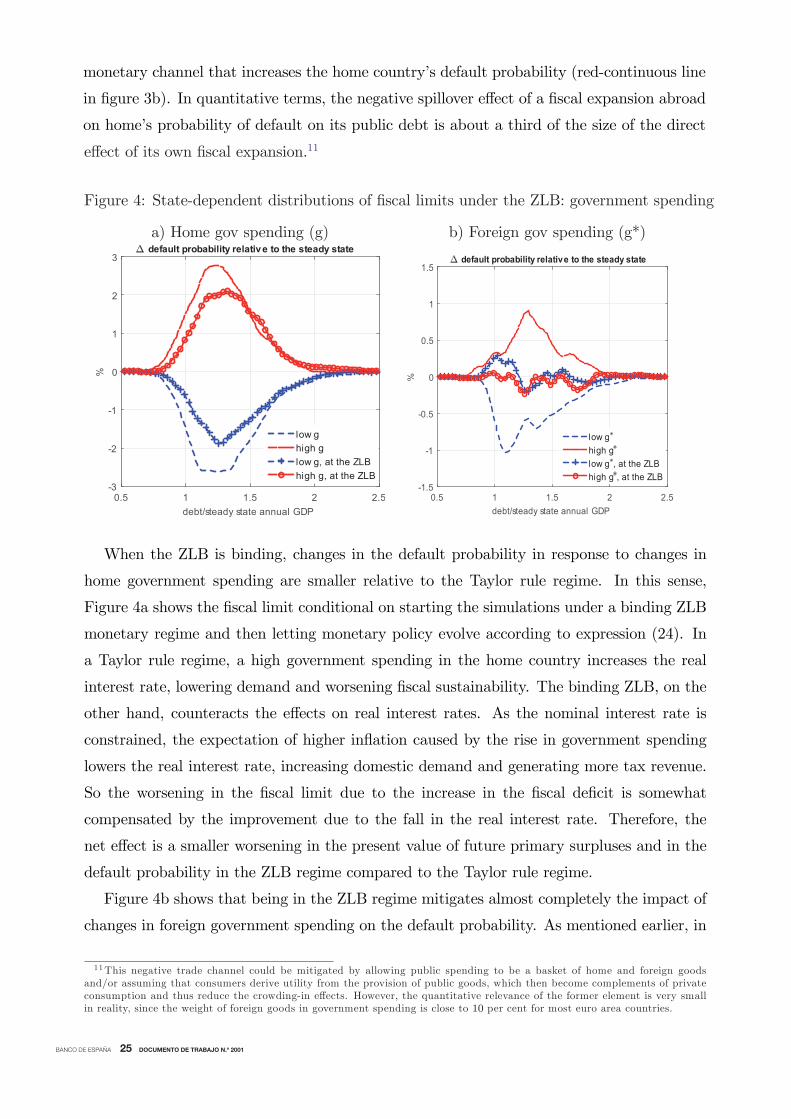
monetary channel that increases the home country’s default probability (red-continuous line
in figure 3b). In quantitative terms, the negative spillover effect of a fiscal expansion abroad
on home’s probability of default on its public debt is about a third of the size of the direct
11This negative trade channel could be mitigated by allowing public spending to be a basket of home and foreign goodsand/or assuming that consumers derive utility from the provision of public goods, which then become complements of privateconsumption and thus reduce the crowding-in effects. However, the quantitative relevance of the former element is very smallin reality, since the weight of foreign goods in government spending is close to 10 per cent for most euro area countries.
effect of its own fiscal expansion.11
Figure 4: State-dependent distributions of fiscal limits under the ZLB: government spending
a) Home gov spending (g) b) Foreign gov spending (g*)
debt/steady state annual GDP0.5 1 1.5 2 2.5
%
-3
-2
-1
0
1
2
3 default probability relative to the steady state
low ghigh glow g, at the ZLBhigh g, at the ZLB
debt/steady state annual GDP0.5 1 1.5 2 2.5
%
-1.5
-1
-0.5
0
0.5
1
1.5 default probability relative to the steady state
low ghigh glow g , at the ZLBhigh g , at the ZLB
When the ZLB is binding, changes in the default probability in response to changes in
home government spending are smaller relative to the Taylor rule regime. In this sense,
Figure 4a shows the fiscal limit conditional on starting the simulations under a binding ZLB
monetary regime and then letting monetary policy evolve according to expression (24). In
a Taylor rule regime, a high government spending in the home country increases the real
interest rate, lowering demand and worsening fiscal sustainability. The binding ZLB, on the
other hand, counteracts the effects on real interest rates. As the nominal interest rate is
constrained, the expectation of higher inflation caused by the rise in government spending
lowers the real interest rate, increasing domestic demand and generating more tax revenue.
So the worsening in the fiscal limit due to the increase in the fiscal deficit is somewhat
compensated by the improvement due to the fall in the real interest rate. Therefore, the
net effect is a smaller worsening in the present value of future primary surpluses and in the
default probability in the ZLB regime compared to the Taylor rule regime.
Figure 4b shows that being in the ZLB regime mitigates almost completely the impact of
changes in foreign government spending on the default probability. As mentioned earlier, in

BANCO DE ESPAÑA 26 DOCUMENTO DE TRABAJO N.º 2001
a Taylor rule regime, an increase in foreign’s government spending raises demand for foreign
goods and lowers demand for home goods, which decreases home country’s export. The
negative trade channel is still present and brings up the default probability. However, when
the ZLB is binding, nominal rates do not rise and the negative trade channel is counteracted
by a fall in the real interest rate, making the increase in the default probability smaller.
The impact of the binding ZLB on default probabilities, depends critically on the per-
sistency of the ZLB regime. If the ZLB regime is expected to last for longer, the response
of real interest rates to inflation expectations is augmented and the monetary channel gets
stronger. As we calibrate the average duration of the ZLB regime to be relatively short, the
quantitative impact of the ZLB regime as shown in Figure 4 can be understood as a lower
bound. If the persistency in the ZLB regime were higher, the positive monetary channel
could dominate the negative trade channel after an increase in foreign government spending,
which could even reduce the default probability.
Finally, the exercises of this section confirm our modelling choice to have the home country,
representing a high debt country with the possibility of default, while the foreign country
does not. In particular, we find that the endogenous fiscal limit in our model is relevant
when the home country has a debt level above 80 percent of GDP; beyond that threshold,
fiscal and monetary shocks induce significant changes in the sustainability of home’s public
finances. This is also consistent with the current levels of debt observed in EMU as shown
in Figure 1, which are around 100 percent in Spain, France and Belgium, above 130 percent
in Italy, while close to 60 percent in Germany.
4.4 Exogenous Fiscal Limit
As mentioned in the introduction, previous papers in the literature study the effects of
exogenous fiscal limits in a monetary union. In fact, Corsetti et al. (2013), Corsetti et al.
(2014) and Batini et al. (2018) allow for the possibility of home government default on public
debt that hence pays a risk premium, but such premium only depends on the level of debt
and it does not respond to other dimensions of the economic environment. In these papers
the fiscal limit follows a distribution (normally a logistic or beta) which is a function only
of the country’s debt to GDP ratio. Therefore, a fiscal consolidation in these models only
affects the risk premium through its effects on debt. As this is a slow moving predetermined
variable, the risk premium cannot jump at the time of the announcement of a policy based on
the expected future fiscal developments. To compare our setting to the previous literature,
although the fiscal limit is model-based, we map the simulated unconditional fiscal limit (as
shown in Figure 2b) to a logistic function, which we use as an exogenous fiscal limit. In
terms of our default equation, 3, this is equivalent to making BH() a logistic function of bt−1.
BANCO DE ESPAÑA 27 DOCUMENTO DE TRABAJO N.º 2001
12The debt rule of the SGP requires a reduction of 1/20th of the distance with 60 per cent each period.
We name this version of the model the "exogenous fiscal limit" case. Finally, to compare
our results to those obtained from a model without risk premium, we set δ = 0 in equation
3, which we name "no default case".
5 Fiscal policy in a monetary union
We now present several fiscal policy exercises with the full non-linear model incorporating
the state-dependent fiscal limit discussed in the previous section arising from the possibility
of the home country government to default on its debt. We concentrate on fiscal issues since
these are very much in the current policy debate in the monetary union and it is precisely
the economic policy where a state-dependent fiscal limit ought to be more relevant. First, we
analyze the long-term process of public deleveraging that is required for high-debt countries
to converge back to the target levels set by European authorities and that we consider the
steady state in our calibration. We also study how the speed of fiscal adjustments determines
its cost. Second, we look at the effect of discretionary policy measures along this process
of convergence. In particular, we will show the effect on the economy of a transitory fiscal
consolidation in a member of the euro area with high debt and a fiscal policy coordination
between both countries. These cases are analyzed under two alternative assumptions about
the monetary policy space in the union depending on whether the Taylor rule is operative or
the economy is temporarily stuck at the zero lower bound so that the nominal interest rate
cannot be reduced any further.
5.1 Long-run fiscal consolidation at home
One of the current main challenges in the euro area is for high debt countries to converge
back towards more sustainable debt levels. In fact, the Stability and Growth Pact (SGP)
sets a limit of 60 percent of GDP for public debt, beyond which the debt rule is active.12
Given the high level of government debt in many countries, this implies a long-term process
of consolidation, which could take several decades, and which will affect the area as a whole.
This process is the focus of this section.
As shown in the previous section, the state-dependent fiscal limit becomes relevant when
debt-to-GDP ratio is around 100 percent, but the steady state debt in both members of the
euro area is 60 percent of GDP. Therefore, the policy relevant exercises have to be based on
an scenario with high debt in the home country, while the foreign country is at its steady
state. In particular, to achieve this we set the initial stock of home debt (bt−1) to 100 percent
of GDP at the beginning of the scenario (t = 0), which generates a risk premium of almost
BANCO DE ESPAÑA 28 DOCUMENTO DE TRABAJO N.º 2001
13This approach provides a good approximation to the true high debt scenario, since although in our model terms of tradein the previous period (tott−1) is also a state variable, endogenizing it would have only a negligible effect.
80 basis points, and then, we let the fiscal and monetary rules bring the economy back to its
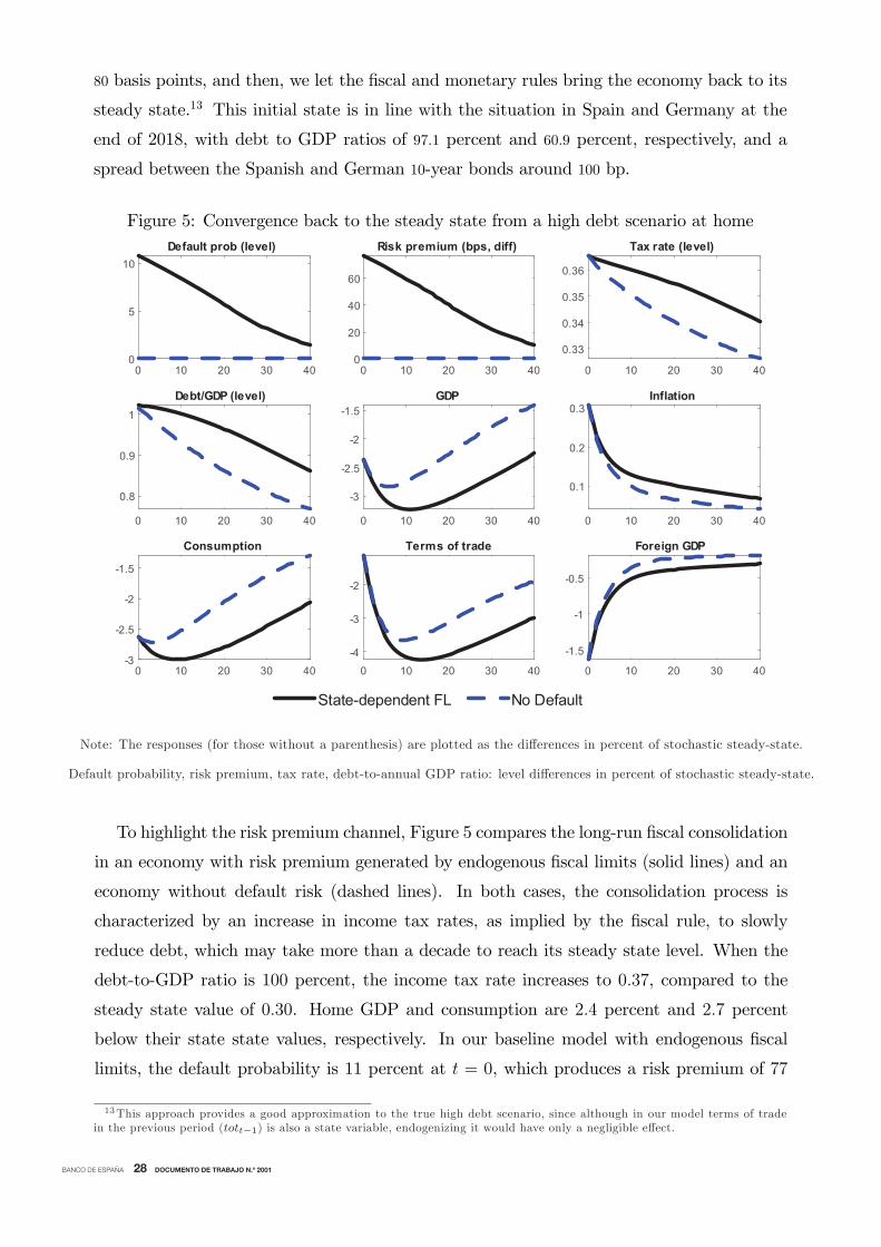
steady state.13 This initial state is in line with the situation in Spain and Germany at the
end of 2018, with debt to GDP ratios of 97.1 percent and 60.9 percent, respectively, and a
spread between the Spanish and German 10-year bonds around 100 bp.
Figure 5: Convergence back to the steady state from a high debt scenario at home
0 10 20 30 400
5
10Default prob (level)
0 10 20 30 400
20
40
60
Risk premium (bps, diff)
0 10 20 30 40
0.33
0.34
0.35
0.36
Tax rate (level)
0 10 20 30 40
0.8
0.9
1
Debt/GDP (level)
0 10 20 30 40
-3
-2.5
-2
-1.5GDP
0 10 20 30 40
0.1
0.2
0.3Inflation
0 10 20 30 40-3
-2.5
-2
-1.5
Consumption
0 10 20 30 40-4
-3
-2
Terms of trade
State-dependent FL No Default
0 10 20 30 40
-1.5
-1
-0.5
Foreign GDP
Note: The responses (for those without a parenthesis) are plotted as the differences in percent of stochastic steady-state.
Default probability, risk premium, tax rate, debt-to-annual GDP ratio: level differences in percent of stochastic steady-state.
To highlight the risk premium channel, Figure 5 compares the long-run fiscal consolidation
in an economy with risk premium generated by endogenous fiscal limits (solid lines) and an
economy without default risk (dashed lines). In both cases, the consolidation process is
characterized by an increase in income tax rates, as implied by the fiscal rule, to slowly
reduce debt, which may take more than a decade to reach its steady state level. When the
debt-to-GDP ratio is 100 percent, the income tax rate increases to 0.37, compared to the
steady state value of 0.30. Home GDP and consumption are 2.4 percent and 2.7 percent
below their state state values, respectively. In our baseline model with endogenous fiscal
limits, the default probability is 11 percent at t = 0, which produces a risk premium of 77

BANCO DE ESPAÑA 29 DOCUMENTO DE TRABAJO N.º 2001
basis points. Although the initial states for the real macroeconomic variables are the same
between the two economies, higher risk premium increases the interest burden on debt and
produces significant differences in the long run. After ten years, the negative output gap in
the economy with risk premium is almost twice as large as the economy without default risk.
In the case with risk premium, debt-to-GDP ratio and tax rates are higher for all periods
while consumption is lower. This worsens the terms of trade and further deprives activity.
The fiscal adjustment in the high-debt economy also spills over to the rest of the euro area,
where foreign output falls persistently.
a) Frontloading vs gradualism b) State-dependent FL vs no default
0 10 20 30 40
2
4
6
8
10Default prob (level)
0 10 20 30 40
20
40
60
Risk premium (bps, diff)
0 10 20 30 40
0.34
0.36
0.38Tax rate (level)
0 10 20 30 40
0.8
0.9
1
Debt/GDP (level)
0 10 20 30 40
-3.5
-3
-2.5
-2
GDP
0 10 20 30 40
0.1
0.2
0.3
0.4
Inflation
0 10 20 30 40-3.5
-3
-2.5
-2
Consumption
0 10 20 30 40
-4
-3
-2
Terms of trade
Baseline ( = 0.04 ) Frontloaded ( = 0.05 )
0 10 20 30 40-2
-1.5
-1
-0.5
Foreign GDP
0 10 20 30 40
-0.5
0
0.5GDP
0 10 20 30 40
-5
0
5
10
1510-3 Tax rate (level)
0 10 20 30 40-0.1
-0.05
0Debt/GDP (level)
State-dependent FLNo default
Note: See Figure 6 for units of y-axes. RHS panel: difference between the frontloaded consolidation (γ= 0.05)
and the gradual consolidation (γ= 0.04).
The long term convergence back towards the 60 percent level of debt will be different
depending on the intensity of the consolidation process, which in our model is driven by the
parameter of debt on the fiscal rule (γ). The presence of a risk premium at high levels of
public debt, speaks in favor of a quicker consolidation to reduce the effective borrowing rate,
nevertheless, that does not imply that fast consolidations are going to be less painful. As
Figure 6a shows, if the country undertakes a faster tax-based consolidation program, which
we model as a fiscal rule with γ = 0.05, the GDP loss is not necessarily lower, despite the
fact that the government manages to reduce the risk premium much faster. The debt-to-
output ratio falls quicker when the consolidation is more frontloaded (γ is higher) and the
Figure 6: Increasing the speed of convergence back to the steady state from a high debt
scenario at home.

BANCO DE ESPAÑA 30 DOCUMENTO DE TRABAJO N.º 2001
risk premium returns to zero after roughly seven years, two-thirds of the time it needs to do
so with a more backloaded consolidation (γ = 0.04). As the income tax rate is higher to retire
debt sooner, in the frontloaded scenario it has a more negative effect on consumption and
GDP, at least in the short to medium run. This is reversed after five years, but the burden
of the short run cost carries a high weight.
Nevertheless, the presence of the fiscal limit implies that increasing the speed of consol-
idation is less painful in an economy with a binding fiscal limit, than in a similar economy
operating further away from the fiscal limit.14 Figure 6b shows that in the latter case (dashed
blue line) speeding up the consolidation process induces a larger and more persistent GDP
fall relative to the more gradual consolidation, than it does in the economy operating close
to the endogenous fiscal limit. In particular, the frontloaded consolidation induces and ad-
ditional cost in terms of GDP losses that lasts 2 years longer (6.5 vs 4.5 years) in the case
of a high debt economy operating away from its fiscal limit than in the one where the limit
is binding. This is due to the fact that the more frontloaded consolidation in the economy
with the binding fiscal limit reduces significantly more the risk premium, which allows for a
quicker reduction in the debt to GDP ratio and in the tax rate.
5.2 Discretionary fiscal consolidation at home
To see how government indebtedness matters for discretionary fiscal consolidation effects in
the home country, we examine an exogenous government spending cut for different levels of
debt, first in the normal (Taylor rule) monetary regime and then when the economy hits
the ZLB. The impulse responses shown in this section represent marginal effects. That is,
the differential impact when we add a transitory spending cut to the baseline long-term
consolidation process described in the previous section. In practice, this means that before
the spending cut, the high-debt state at t = 0 is simulated like in the previous section
(the low-debt state is the stochastic steady state of 60 percent) and an additional 1 percent
negative government spending shock is injected at t = 0.
14For the sake of simplicity we model the latter case as an economy where there is no default, so that its risk-premium is notaffected by the level or the speed of debt reduction. This would be equivalent to a high-debt economy for which the fiscal limitis high enough so that reaching a debt level of 100% of GDP does not to increase significantly the risk-premium.
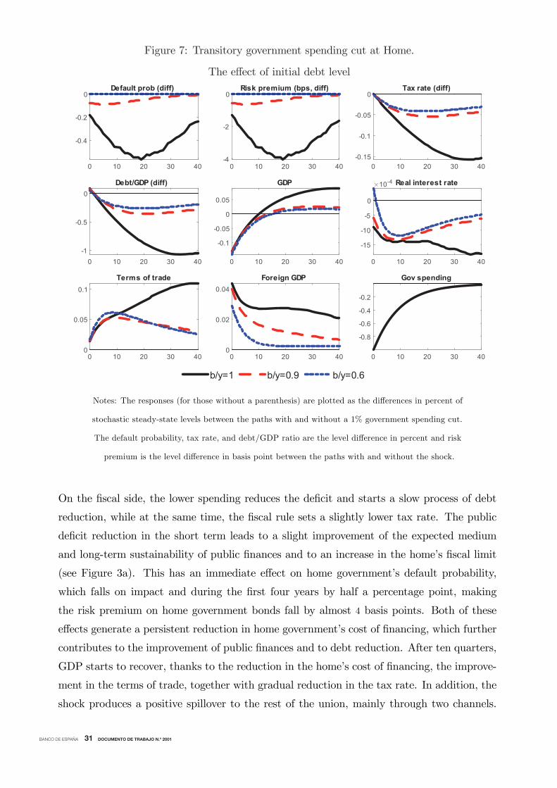
Solid lines in Figure 7 show the macroeconomic responses to a 1 percent transitory gov-
ernment spending cut in a high-debt member of a monetary union. Discretionary fiscal
consolidation reduces output and inflation on impact due to lower demand for domestic
goods. The real interest rate falls immediately by 10bp and then slowly gets more negative.
Since the home country has a small weight in the Taylor rule, the initial impact on the
EA wide nominal interest rate is contained and so is the impact on the real interest rate,
but as the output gap is closed, inflation recovers and the real rate falls more significantly.
BANCO DE ESPAÑA 31 DOCUMENTO DE TRABAJO N.º 2001
Figure 7: Transitory government spending cut at Home.
The effect of initial debt level
0 10 20 30 40
-0.4
-0.2
0Default prob (diff)
0 10 20 30 40-4
-2
0Risk premium (bps, diff)
0 10 20 30 40-0.15
-0.1
-0.05
0Tax rate (diff)
0 10 20 30 40-1
-0.5
0Debt/GDP (diff)
0 10 20 30 40
-0.1
-0.05
0
0.05
GDP
0 10 20 30 40
-15
-10
-5
0
10-4 Real interest rate
0 10 20 30 400
0.05
0.1
Terms of trade
0 10 20 30 400
0.02
0.04Foreign GDP
b/y=1 b/y=0.9 b/y=0.6
0 10 20 30 40
-0.8
-0.6
-0.4
-0.2
Gov spending
Notes: The responses (for those without a parenthesis) are plotted as the differences in percent of
stochastic steady-state levels between the paths with and without a 1% government spending cut.
The default probability, tax rate, and debt/GDP ratio are the level difference in percent and risk
premium is the level difference in basis point between the paths with and without the shock.
On the fiscal side, the lower spending reduces the deficit and starts a slow process of debt
reduction, while at the same time, the fiscal rule sets a slightly lower tax rate. The public
deficit reduction in the short term leads to a slight improvement of the expected medium
and long-term sustainability of public finances and to an increase in the home’s fiscal limit
(see Figure 3a). This has an immediate effect on home government’s default probability,
which falls on impact and during the first four years by half a percentage point, making
the risk premium on home government bonds fall by almost 4 basis points. Both of these
effects generate a persistent reduction in home government’s cost of financing, which further
contributes to the improvement of public finances and to debt reduction. After ten quarters,
GDP starts to recover, thanks to the reduction in the home’s cost of financing, the improve-
ment in the terms of trade, together with gradual reduction in the tax rate. In addition, the
shock produces a positive spillover to the rest of the union, mainly through two channels.

BANCO DE ESPAÑA 32 DOCUMENTO DE TRABAJO N.º 2001
the economic environment. Therefore, a fiscal consolidation does not trigger an immediate
fall in the risk premium upon the policy implementation, but instead the risk premium is
reduced slowly as debt falls.
In the model without default risk, reducing public debt does not affect the cost of financing
and therefore, the impulse responses look very similar to the ones under a scenario of low
In order to study more closely the role of the risk premium in the transmission channel
of fiscal shocks. In Figure 8, we compare our model with the two alternative ones previously
used in the literature and explained in the previous section: dashed-dotted red lines depict
the effect of a fiscal consolidation at home in a standard model without default risk, while
the dashed blue lines show the effect in a model with an exogenous fiscal limit (see Davig
et al. (2010), Corsetti et al. (2013), Corsetti et al. (2014) and Batini et al. (2018)), in which
there is the possibility of home government default and thus it pays a risk premium, but such
premium only depends on the level of debt and it does not respond to other dimensions of
On the one hand, the fall in activity and inflation at home slightly pushes down the ECB’s
nominal interest rate and fosters economic activity in the rest of the union. On the other
hand, the increase in home’s consumption fosters exports from the rest of the union. This
leads to a small reduction in foreign debt.
As one would expect, our non-linear model is capable of showing that the benefits from
fiscal consolidation are greater when an economy is in a high debt situation than when its
public finances are in better shape. The blue dashed lines of Figure 7 depict the effect of the
same discretionary spending cut starting from a low level of debt (60 percent of GDP, the
stochastic steady state). In this case, home’s government finances are in much better shape
and therefore very far from the fiscal limit, so the risk premium is close to zero and insensitive
to small changes in debt sustainability. Therefore, the discretionary fiscal consolidation
cannot improve the probability of default, which is almost nil, and thus does not reduce the
risk premium. The output recovery does not benefit from lower interest payments on debt
and is therefore much weaker, resulting in a smaller reduction in public debt. The positive
spillover effect to the rest of the union, is also smaller. On the contrary, as the initial level of
debt gets higher, red dashed-dotted lines represent a 90 percent debt-GDP ratio, the impact
of a spending cut on the risk premium starts to have a more significant effect. Moreover,
comparing the three cases shows clearly that the effect of the fiscal limit on real activity is
very non-linear, increasing very quickly as the high-debt country approaches the fiscal limit.
In this sense, it is worth reminding that it does no take a very high probability of reaching
the fiscal limit for it to become relevant. According to Figure 2, with a debt to GDP ratio
of 100 percent, the economy has barely a 10 percent probability of default on the service of
the debt.

BANCO DE ESPAÑA 33 DOCUMENTO DE TRABAJO N.º 2001
Key in the outcome of these consolidation scenarios is the monetary regime the union
finds itself in. Figure 9 compares our baseline simulation, with an alternative monetary
Figure 8: Transitory government spending cut at Home.
The effect of a state-dependent risk premium
0 10 20 30 40
-0.4
-0.2
0Default prob (diff)
0 10 20 30 40-4
-2
0Risk premium (bps, diff)
0 10 20 30 40-0.15
-0.1
-0.05
0Tax rate (diff)
0 10 20 30 40-1
-0.5
0Debt/GDP (diff)
0 10 20 30 40
-0.1
-0.05
0
0.05
GDP
0 10 20 30 40
-1.5
-1
-0.5
010-3 Real interest rate
0 10 20 30 400
0.05
0.1
Terms of trade
0 10 20 30 400
0.02
0.04Foreign GDP
baseline no default exogenous FL
0 10 20 30 40
-0.8
-0.6
-0.4
-0.2
Gov spending
Notes: See Figure 8 for units of y-axes.
debt. In the model with exogenous fiscal limits, the fiscal consolidation increases government
primary surplus and lowers debt gradually. As public debt adjusts back to its steady state
level, the default probability and risk premium decrease slowly, as shown by the dashed blue
line. In our model with state-dependent fiscal limits, the discretionary spending cut improves
the home government’s fiscal outlook and immediately pushes the fiscal limit distribution to
the right, improving the home government’s debt sustainability. This in turn makes the risk
premium jump down on impact, shortening the initial recession and increasing the strength
of the recovery. With state-dependent fiscal limits, the decrease in risk premium is almost 2
basis points more than that with exogenous fiscal limits throughout the horizon. These small
variations in risk premium can produce significant differences in debt dynamics. After ten
years, annual debt-to-GDP ratio decreases by 1.08 percentage points with state-dependent
fiscal limits, compared to 0.76 with exogenous fiscal limits. In addition, the more powerful
risk premium channel in our model increases the positive spillover effect to the rest of the
union.

BANCO DE ESPAÑA 34 DOCUMENTO DE TRABAJO N.º 2001
policy regime at the ZLB. On impact, the reduction in default probability and risk premium
under the ZLB regime are smaller than that under the Taylor rule regime, consistent with the
fiscal limit distribution in Figure 2b. For the longer horizon, a persistent fiscal consolidation
generates deflation expectations. When the nominal interest rate is constrained at zero, the
real interest rate is consistently higher than that under the Taylor rule regime. Higher real
interest rates lower demand, increase the cost of servicing the debt, mitigating the strength
of the risk premium channel explained before. Therefore, under the ZLB the presence of
Figure 9: Transitory government spending cut at Home.
The effect of binding ZLB
0 10 20 30 40
-0.4
-0.2
0Default prob (diff)
0 10 20 30 40-4
-2
0Risk premium (bps, diff)
0 10 20 30 40-0.15
-0.1
-0.05
0Tax rate (diff)
0 10 20 30 40-1
-0.5
0
Debt/GDP (diff)
0 10 20 30 40
-0.1
-0.05
0
0.05
GDP
0 10 20 30 40
0
2
4
6
10-3 Real interest rate
0 10 20 30 400
0.05
0.1
Terms of trade
0 10 20 30 400
0.02
0.04Foreign GDP
Normal times ZLB
0 10 20 30 40
-0.8
-0.6
-0.4
-0.2
Gov spending
Notes: See Figure 8 for units of y-axes.
an state-dependent fiscal limit does not make fiscal consolidations as beneficial as they are
when monetary policy operates under a Taylor rule.
Table 2 reports the cumulative government spending multipliers for output in the home
country, foreign country, and the Euro area for various models, computed as
ki=0
i
j=0
rt+j−1 xt+i
ki=0
i
j=0
rt+j−1 gt+i
, x ∈ {y, y∗, yMU}, (33)

BANCO DE ESPAÑA 35 DOCUMENTO DE TRABAJO N.º 2001
The fiscal multiplier, measuring the reduction in output due to a 1 euro fall in government
spending, is similar the first year after the shock (see rows 1 and 4 of the top panel in Table 2)
without or with default risk, but the difference can be sizable in the medium to long run. The
ten year cumulative fiscal multiplier after a discretionary government spending cut in a model
without sovereign default is 0.24, it changes its sign, becoming expansionary (−0.24) when
default is introduced through exogenous fiscal limits, while the fiscal consolidation becomes
more expansionary (−0.5), when a state-dependent fiscal limit is considered. Having fiscal
limits respond directly to the economic states amplifies the risk premium channel and makes
fiscal consolidation more expansionary for the home country in the long run. For the Euro
area, consolidation in the highly-indebted country also results in long run gains. The ten-
year multiplier for the Euro area is −0.45 with state-dependent fiscal limits, compared to
−0.08 in the model without default. A binding ZLB, on the other hand, mitigates the risk
where denotes level changes relative to a path without government spending changes. To
keep the comparison consistent among different models, we use rt = β−1 as the real interest
rate.
Table 2: Output multipliers from a discretionary government spending cut at home
Periphery (home) Spillover to core (foreign) Euro area
Multiplier PV (Δy)PV (Δg)
PV (Δy∗)PV (Δg)
PV (ΔyMU )PV (Δg)
Models 0 yr 1 yr 5 yr 10 yr 0 yr 1 yr 5 yr 10 yr 0 yr 1 yr 5 yr 10 yr
No default 0.71 0.66 0.44 0.24 -0.18 -0.17 -0.21 -0.25 0.14 0.13 0.03 -0.08
Exogenous FL 0.71 0.66 0.31 -0.24 -0.18 -0.18 -0.26 -0.37 0.14 0.12 -0.05 -0.32
State-dependent FL 0.71 0.65 0.23 -0.50 -0.18 -0.18 -0.28 -0.42 0.14 0.12 -0.10 -0.45
State-dependent FL, ZLB 0.82 0.77 0.63 0.56 -0.09 -0.08 -0.07 -0.09 0.23 0.22 0.18 0.15
premium channel by weakening demand through a higher real interest rate. The monetary
channel can be sizeable, in which the ten-year multiplier for the home country reverses its
sign, from −0.5 to 0.56.
5.3 Discretionary fiscal coordination
Following the sovereign debt crises in the euro area, a consensus has emerged about the need
of a coherent and integrated fiscal policy strategy to ensure growth and debt sustainability. A
pertinent question is whether the various fiscal policies at the national levels are complements
or substitutes. In this section, we consider two fiscal policy coordination plans and compare
them with the discretionary home consolidation in the previous section.

BANCO DE ESPAÑA 36 DOCUMENTO DE TRABAJO N.º 2001
Figure 10 plots the macroeconomic effects of three fiscal policy combinations: A 1 percent
Figure 10: Fiscal policy coordination: Taylor rule regime.
0 10 20 30 40-0.6
-0.4
-0.2
Default prob (diff)
0 10 20 30 40
-4
-3
-2
-1Risk premium (bps, diff)
0 10 20 30 40
-0.15
-0.1
-0.05
Tax rate (diff)
0 10 20 30 40
-1
-0.5
0
Debt/GDP (diff)
0 10 20 30 40
-0.1
0
0.1GDP
0 10 20 30 40
-4
-2
0
2
10-3 Real interest rate
0 10 20 30 400
0.05
0.1
Terms of trade
0 10 20 30 40-0.1
0
0.1
Foreign GDP
0 10 20 30 40
-0.05
0
0.05
Union GDP
Home consolidation Home consolidation & Foreign expansion Both consolidation
Notes: See Figure 8 for units of y-axes.
government spending cut in the high debt home country (solid lines), a 1 percent government
spending cut in the high debt home country and a 1 percent government spending increase in
the low debt foreign country (dashed lines), and a 1 percent government spending cut in both
countries (dashed-dotted lines). In the short run, fiscal expansions in the foreign country
increase foreign GDP and union-wide inflation rate, pushing up real interest rates in both
countries. As a consequence home GDP decreases, but given the large size of the foreign
country, the union GDP improves. Moreover, the higher real interest rates worsen debt
sustainability in the home country, increasing default probabilities and the risk premium.
This effect partially compensates the reduction of risk premium from home consolidation and
lowers home GDP relative to the case without foreign fiscal expansions. After year three,
when the initial positive effects on the foreign GDP fade away, the negative effects on home
GDP start to dominate, and the union-wide GDP becomes lower with foreign expansion than
otherwise without one. The little spillover on home activity from a foreign fiscal expansion
is partly due to the weak trade channel present in this model. This could be mitigated by
allowing public spending to be a basket of home and foreign goods and/or assuming that
consumers derive utility from the provision of public goods, which then become complements
of private consumption and thus reduce the crowding-in effects.
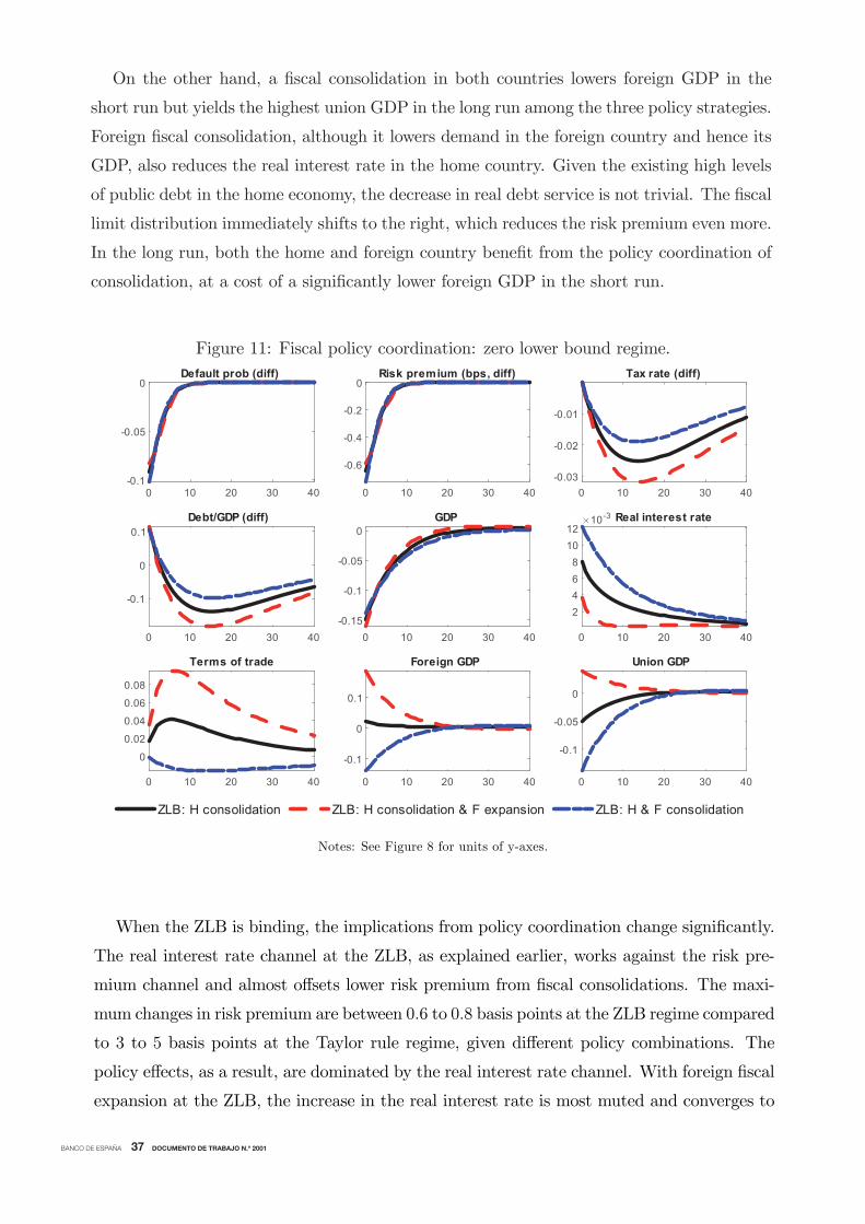
BANCO DE ESPAÑA 37 DOCUMENTO DE TRABAJO N.º 2001
On the other hand, a fiscal consolidation in both countries lowers foreign GDP in the
short run but yields the highest union GDP in the long run among the three policy strategies.
Foreign fiscal consolidation, although it lowers demand in the foreign country and hence its
GDP, also reduces the real interest rate in the home country. Given the existing high levels
of public debt in the home economy, the decrease in real debt service is not trivial. The fiscal
limit distribution immediately shifts to the right, which reduces the risk premium even more.
In the long run, both the home and foreign country benefit from the policy coordination of
consolidation, at a cost of a significantly lower foreign GDP in the short run.
When the ZLB is binding, the implications from policy coordination change significantly.
The real interest rate channel at the ZLB, as explained earlier, works against the risk pre-
mium channel and almost offsets lower risk premium from fiscal consolidations. The maxi-
mum changes in risk premium are between 0.6 to 0.8 basis points at the ZLB regime compared
to 3 to 5 basis points at the Taylor rule regime, given different policy combinations. The
policy effects, as a result, are dominated by the real interest rate channel. With foreign fiscal
expansion at the ZLB, the increase in the real interest rate is most muted and converges to
Figure 11: Fiscal policy coordination: zero lower bound regime.
0 10 20 30 40-0.1
-0.05
0Default prob (diff)
0 10 20 30 40
-0.6
-0.4
-0.2
0Risk premium (bps, diff)
0 10 20 30 40-0.03
-0.02
-0.01
Tax rate (diff)
0 10 20 30 40
-0.1
0
0.1Debt/GDP (diff)
0 10 20 30 40-0.15
-0.1
-0.05
0GDP
0 10 20 30 40
2468
1012
10-3 Real interest rate
0 10 20 30 40
0
0.02
0.04
0.06
0.08
Terms of trade
0 10 20 30 40
-0.1
0
0.1
Foreign GDP
0 10 20 30 40
-0.1
-0.05
0
Union GDP
ZLB: H consolidation ZLB: H consolidation & F expansion ZLB: H & F consolidation
Notes: See Figure 8 for units of y-axes.

BANCO DE ESPAÑA 38 DOCUMENTO DE TRABAJO N.º 2001
zero after five quarters, producing the largest expansionary effect union wide. This result
is in line with previous findings in the literature. Blanchard et al. (2017) show that a fiscal
expansion by the core economies of the euro area would have a large and positive impact on
periphery GDP assuming that policy rates remain low for a prolonged period. Arce et al.
(2016) find that a fiscal expansion in the core aggravates the recession in the periphery, due
to higher real rates, but the cross-country spillovers are reversed in a liquidity trap. There-
fore, our results extend the previous findings to show that even in the presence of a fiscal
limit the fiscal policy spillovers depend critically on the monetary policy regimes.
6 Concluding remarks
In this paper we study the effects of fiscal policy and its spillovers for countries in a monetary
union with different levels of public debt. We develop a dynamic stochastic general equilib-
rium model of a two-country monetary union in which country members have substantially
different debt to GDP ratios. These two countries are calibrated to match the characteristics
of Spain and Germany respectively. Only the high-debt country (100 percent of GDP) faces
some probability of default on the service of its debt. This probability is endogenous and
default occurs when current outstanding real debt in period t is higher than the maximum
amount of public debt that the government can finance without defaulting on their financial
commitments or fiscal limit. This fiscal limit is calculated as the expected discounted sum
of maximum primary surplus that can be generated in the future, given the current fiscal
strategy and the expected evolution of the economy. Since this evolution is uncertain this
gives rise to a distribution of values of the maximum sustainable level of debt out of which
a particular value is drawn as the stochastic fiscal limit.
Policy changes affect now the economy in two ways. One is the standard transmission
mechanism built in the DSGE model, the other is the change in the market’s expectation
about future primary surplus, which has a direct effect on the fiscal limit distribution and
hence on the probability of default and on the current sovereign risk premium. This adds a
new channel to the macroeconomic responses to policy (or otherwise) shocks.
We find that the fiscal permanent consolidation necessary to bring a high-debt country
back to more sustainable debt levels within a monetary union is very costly in terms of output
loss not only for the consolidating country, but also for the other members of the union. The
fact that high debt makes it more likely to hit the fiscal limit introduces an additional cost
to high-debt countries in the form of a risk premium in the interest rate that affects both the
government and the private sector spending decisions. In these circumstances, frontloaded
(faster) public debt consolidations are still more costly than more gradual ones in terms of

BANCO DE ESPAÑA 39 DOCUMENTO DE TRABAJO N.º 2001
not facing a risk premium.
In normal times, when monetary policy is run according to a standard Taylor rule, tran-
sitory government spending cuts in the high-debt country enlarge the fiscal space of the
economy, reduce risk premium and facilitate a faster recovery of output, as compared with
what would happen in a low-debt economy. In such a case, the short-term improvement in
public finances of a high-debt country reduces its risk premium on impact and thereafter,
making the output costs of consolidating much smaller. Moreover, this effect may be quanti-
tatively relevant as the long-term multipliers of government spending are greatly reduced by
this risk premium channel, and may even change sign. This effect is highly non linear; it is
hardly significant when the economy starts from a debt to GDP ratio below 90 percent, and
increases rapidly beyond 100 percent. On the contrary, a fiscal expansion in a high debt coun-
try, even of a transitory character, in our model will significantly increase the risk-premium
undoing most of the direct output gains derived from the increase in government spending.
In terms of fiscal coordination within the monetary union, the best strategy in a normal
monetary regime is for both members to consolidate simultaneously since this decreases real
interest rates and amplifies the reduction in risk premium in the highly-indebted country,
improving union-wide output in the long run, but at the cost of lower output in the low-debt
country in the short term.
On the contrary, when monetary policy is constrained at the zero lower bound, the risk
premium channel arising from endogenous fiscal limits and driving all the previous results
becomes muted, making the costs of consolidation very similar across the high and low debt
economies within the monetary union. If monetary policy is constrained in this way the real
interest rate moves in opposite direction than the inflation rate, which may offset partially or
completely the response of the risk premium. In this context, the best coordination strategy
is for the low-debt country to expand government spending and for the high-debt country
to consolidate.
In future work we would like to explore how our results are affected under two different
environments. First, what happens when some of the risk sharing mechanisms available
within a monetary union and currently under discussion in the policy debate. In particular,
it would be interesting to extend the model to allow for cross border purchases of sovereign
debt, the introduction of a Eurobond or the creation of a fiscal capacity at the EMU level to
smooth the effects of asymmetric shocks. Second, what happens when a part of government
expenditure is of a productive nature and thus affects positively the supply-side of the econ-
GDP and consumption loss, but this extra cost is smaller than what would be in an economy
omy. In this case, the impact on the fiscal limit from the worsening of public finances due

BANCO DE ESPAÑA 40 DOCUMENTO DE TRABAJO N.º 2001
to the fiscal expansion may be partially compensated by the improvement in productivity.
This trade-off may change the results of the policy coordination exercises described in this
paper and is a policy option currently very prominent in the debate of fiscal coordination
within EMU.
BANCO DE ESPAÑA 41 DOCUMENTO DE TRABAJO N.º 2001
References
Aguiar, M. and G. Gropinath (2006). Defaultable debt, interest rates and the current account. Journal of
International Economics 69, 64—83.
Alesina, A. and S. Ardagna (2010). Large changes in fiscal policy: Taxes versus spending. Tax Policy and
the Economy 24 (1), 35—68.
Alesina, A., S. Ardagna, and J. Galí (1998). Tales of fiscal adjustment. Economic Policy 13 (27), 489—545.
Alvarez, L. J., E. Dhyne, M. Hoeberichts, C. Kwapil, H. Bihan, P. LÃijnnemann, F. Martins, R. Sabbatini,
H. Stahl, P. Vermeulen, and J. Vilmunen (2006). Sticky prices in the euro area: A summary of new
micro-evidence. Journal of the European Economic Association 4 (3), 575—584.
Arce, O., S. Hurtado, and C. Thomas (2016). Policy spillovers and synergies in a monetary union. Interna-
tional Journal of Central Banking 12 (3), 219—277.
Arellano, C. (2008). Default risk and income fluctuations in emerging economies. American Economic
Review 98 (3), 690—712.
Ascari, G. and L. Rossi (2012). Trend inflation and firms price-setting: Rotemberg versus calvo. The
Economic Journal 122 (563), 1115—1141.
Batini, N., G. Melina, and S. Villa (2018). Fiscal buffers, private debt, and recession: The good, the bad
and the ugly. Journal of Macroeconomics.
Battistini, N., G. Callegari, and L. Zavalloni (2019). Dynamic fiscal limits and monetary-fiscal policy inter-
actions. ECBF Working Paper No. 2268.
Benigno, G. and P. Benigno (2006). Designing targeting rules for international monetary policy cooperation.
Journal of Monetary Economics 53 (3), 473—506.
Bi, H. (2012). Sovereign default risk premia, fiscal limits, and fiscal policy. European Economic Review 56 (3),
389—410.
Bi, H., E. M. Leeper, and C. Leith (2018). Sovereign default and monetary policy tradeoffs. International
Journal of Central Banking . forthcoming.
Bi, H., W. Shen, and S.-C. S. Yang (2016). Fiscal limits in developing countries: A DSGE approach. Journal
of Macroeconomics 49, 119—130.
Blanchard, O., C. J. Erceg, and J. Linde (2017). Jump-starting the euro-area recovery: Would a rise in core
fiscal spending help the periphery? NBER Macroeconomics Annual 31 (1), 103—182.
BANCO DE ESPAÑA 42 DOCUMENTO DE TRABAJO N.º 2001
Blanchard, O. J. (2019). Public debt and low interest rates. American Economic Review 109 (4), 1197—1229.
Chari, V. V., A. Dovis, and P. J. Kehoe (2019). Rethinking optimal currency areas. Journal of Monetary
Economics.
Coleman, II, W. J. (1991). Equilibrium in a production economy with an income tax. Econometrica 59 (4),
1091—1104.
Corsetti, G., K. Kuester, A. Meier, and G. J. Muller (2013). Sovereign risk, fiscal policy, and macroeconomic
stability. The Economic Journal 123 (566), 99—132.
Corsetti, G., K. Kuester, A. Meier, and G. J. Muller (2014). Sovereign risk and belief-driven fluctuations in
the euro area. Journal of Monetary Economics 61, 53—73.
Corsetti, G., A. Meier, and G. J. Muller (2010). Cross-border spillovers from fiscal stimulus. International
Journal of Central Banking 6 (1), 5—37.
Daniel, B. C. and C. Shiamptanis (2012). Fiscal risk in a monetary union. European Economic Review 56 (6),
1289—1309.
Davig, T. (2004). Regime-switching debt and taxation. Journal of Monetary Economics 51 (4), 837—859.
Davig, T., E. M. Leeper, and T. B. Walker (2010). Unfunded liabilities and uncertain fiscal financing. Journal
of Monetary Economics 57 (5), 600—619.
Dovis, A. (2019). Efficient sovereign default. The Review of Economic Studies 86 (1), 282—312.
Eaton, J. and M. Gersovitz (1981). Debt with potential repudiation: Theoretical and empirical analysis.
Review of Economic Studies 48 (2), 289—309.
European Commission (2018). Taxation trends in the European Union. European Union.
Fabiani, S., M. Druant, I. Hernando, C. Kwapil, B. Landau, C. Loupias, F. Martins, T. Matha, R. Sabbatini,
H. Stahl, and A. C. J. Stokman (2005). The pricing behaviour of italian firms: new survey evidence on
price stickiness. ECB working paper No. 535, October 2005.
Farhi, E. and I. Werning (2016). Fiscal Multipliers: Liquidity Traps and Currency Unions, Volume 2, Book
section 31, pp. 2417—2492. Elsevier.
Gadatsch, N., K. Hauzenberger, and N. Stähler (2015). Germany and the rest of euro area fiscal policy
during the crisis. Discussion Paper No. 05/2015, Deutsche Bundesbank.
Garcia-Cicco, J., R. Pancrazi, and M. Uribe (2010). Realbusiness cycles inemerging countries? American
Economic Review 100 (5), 2510—31.

BANCO DE ESPAÑA 43 DOCUMENTO DE TRABAJO N.º 2001
Giavazzi, F. and M. Pagano (1990). Can severe fiscal contractions be expansionary? tales of two small
european countries. NBER Macroeconomics Annual 5, 75—111.
Gil, M., J. J. Pérez, and A. Urtasun (2017). Macroeconomic uncertainty: measurement and impact on the
Spanish economy. Economic Bulletin. Banco de España.
Mendoza, E. G. and V. Z. Yue (2012). A general equilibrium model of sovereign default and business cycles.
The Quarterly Journal of Economics 127 (2), 889—946.
Polito, V. and M. Wickens (2015). Sovereign credit ratings in the european union: A model-based fiscal
analysis. European Economic Review 78, 220—247.
Richter, A. and N. Throckmorton (2015). The zero lower bound: frequency, duration, and numerical con-
vergence. The B.E. Journal of Macroeconomics 15 (1), 157.
Rotemberg, J. J. (1982). Sticky prices in the United States. Journal of Political Economy 90 (6), 1187—1211.
Schmitt-Grohe, S. and M. Uribe (2007). Optimal simple and implementable monetary and fiscal rules.
Journal of Monetary Economics 54 (6), 1702—1725.
Sturzenegger, F. and J. Zettelmeyer (2008). Haircuts: Estimating investor losses in sovereign debt restruc-
turings, 1998-2005. Journal of International Money and Finance 27 (5), 780—805.
Trabandt, M. and H. Uhlig (2011). The laffer curve revisited. Journal of Monetary Economics 58 (4),
305—327.
Uribe, M. and V. Z. Yue (2006). Country spreads and emerging countries: Who drives whom? Journal of
International Economics 69 (1), 6—36.
Vermeulen, P., D. A. Dias, M. Dossche, E. Gautier, I. Hernando, R. Sabbatini, and H. Stahl (2012). Price
setting in the euro area: Some stylized facts from individual producer price data. Journal of Money, Credit
and Banking 44 (8), 1631—1650.
Yue, V. Z. (2010). Sovereign default and debt renegotiation. Journal of International Economics 80, 176—187.

BANCO DE ESPAÑA 44 DOCUMENTO DE TRABAJO N.º 2001
Appendix A Equilibrium
The equilibrium consists of 35 equations (16 for the home country, 14 for the foreign country
and 5 are common), to solve for 35 variables (λt, ct, nt, wt, δt, Rt, τ t, πt, πH,t, mct, yt, bt,
Tt, cHMU,t, Υt, gt for the home country, λ∗t , c
∗t , n
∗t ,w
∗t , τ
∗t , π
∗t , πF,t, mc
∗t , y
∗t , b
∗t , T
∗t , c
FMU,t, Υ
∗t ,
g∗t for the foreign country and tott, RERt, πMU,t, yMU,t, Rft ) for the union.
Home equations
λt = c−σt (A.1)
nϕt = λt(1− τ t)wt (A.2)
Since we have default, we need both the Euler equation under default and under no default
to evaluate the expectation about future defaults
λt = βRftEtλt+1πt+1
(A.3)
λt = βRtEt(1− δt+1)λt+1
πt+1(A.4)
δt =
⎧⎨⎩ 0 if bt−1 < BH(St)
δ if bt−1 ≥ BH(St)(A.5)
πt = πηH,tπ
1−ηF,t (A.6)
mct = tot1−ηt
wta
(A.7)
ψπH,tπ− 1 πH,t
π= (1− θ) + θmct + ψβEt
λt+1λt
πH,t+1π
− 1 yt+1πH,t+1ytπ
(A.8)
1− ψ
2
πH,tπ− 1
2
yt = tot1−ηt cHMU,t + gt (A.9)
cHMU,t = ηct + η∗1− ssc∗t (A.10)
yt = ant (A.11)
Υt = 1−mct −ψ
2
πH,tπ− 1
2
yt (A.12)

BANCO DE ESPAÑA 45 DOCUMENTO DE TRABAJO N.º 2001
btRt+Tt − gttot1−ηt
=(1− δt) bt−1
πt(A.13)
Tt = 1− ψ
2
πH,tπ− 1
2
τ tyt (A.14)
τ t = τ + γb(bt−1 − b) (A.15)
lngtg= ρg ln
gt−1g+ εgt (A.16)
Foreign equations
λ∗t = (c∗t )−σ (A.17)
(n∗t )ϕ = λ∗t (1− τ ∗t )w
∗t (A.18)
In the full model, if there is no default in either country, the risky and risk free rates are
identical and we can use the RERt expression for foreign consumption. If instead home
country sovereign debt is subject to default, while foreign country’s sovereign debt is not,
then the rate of return in foreign is equal to the risk-free rate, but we have to use the foreign
Euler equation to solve the model.
no default in the model (both home and foreign):ctc∗t
σ
= RERt = totη−η∗t (A.19)
default in home but no default in foreign: λ∗t = βRftEtλ∗t+1π∗t+1
(A.20)
π∗t = πη∗H,tπ
1−η∗F,t (A.21)
mc∗t = tot−η∗t
w∗ta∗
(A.22)
ψπF,tπ∗
− 1 πF,tπ∗
= (1− θ) + θmc∗t + ψβEtλ∗t+1λ∗t
πF,t+1π∗
− 1 y∗t+1πF,t+1y∗t π
∗ (A.23)
1− ψ
2
πF,tπ∗
− 12
y∗t = tot−η∗t cFMU,t + g
∗t (A.24)
cFMU,t =s (1− η)
1− s ct + (1− η∗) c∗t (A.25)

BANCO DE ESPAÑA 46 DOCUMENTO DE TRABAJO N.º 2001
y∗t = a∗n∗t (A.26)
Υ∗t = 1−mc∗t −ψ
2
πF,tπ∗
− 12
y∗t (A.27)
b∗t
Rft+ totη
∗t (T
∗t − g∗t ) =
b∗t−1π∗t
(A.28)
T ∗t = 1− ψ
2
πF,tπ∗
− 12
τ ∗ty∗t (A.29)
τ ∗t = τ ∗ + γb(b∗t−1 − b∗) (A.30)
lng∗tg∗= ρg ln
g∗t−1g∗
+ εg∗t (A.31)
Union wide equations
tott = tott−1πF,tπH,t
(A.32)
Rt =
⎧⎪⎪⎨⎪⎪⎩R + απ(πMU,t − πMU), if sRt = 1
1, if sRt = 2(A.33)
yMU,t = syt + (1− s)y∗t (A.34)
πMU,t = sπt + (1− s)π∗t (A.35)
RERt = totη−η∗t (A.36)
Appendix B The Numerical Solution Method
Appendix B.1 Solving the fiscal limit
This appendix describes procedures in simulating fiscal limit distributions. First, derive the
expression of the fiscal limit as (31). Second, replace the fiscal rules (A.15) and (A.30) with
the maximum tax rate τmax and τ ∗max and solve the full model (without default) non-linearly
evaluated at the maximum tax rate.
When solving the nonlinear model without default, the state space is St = gt, g∗t , tott−1, s
Rt ,
depending on the number of exogenous shocks we consider to build the fiscal limit. Since
the model without default has three expectation terms in equations (Euler equation of home
BANCO DE ESPAÑA 47 DOCUMENTO DE TRABAJO N.º 2001
15We do not have an expectation term in the foreign Euler equation because in the model without risk we can use insteadequation (A.20).
country (A.3)15, Phillips curve of home (A.8) and foreign (A.23) we need three decision
rules. It can be shown that these three equations can be written as a function of only
three variables: nt, πH,t and πF,t. Therefore, the decision rule for labor in home country is
nmaxt = fn(St), the rule for inflation of the home goods is πmaxH,t = fπH (St), and the rule for
inflation of the foreign goods is πmaxF,t = fπF (St).
From the converged rules for fn(·), fπH (·), and fπF (·), we derive the rules for the remain-ing variables determining the fiscal limit Tmaxt = fT (St), T ∗maxt = fT ∗(St), λmaxt = fλ(St),λ∗maxt = fλ∗(St), and totmaxt = f tot(St), which are consistent with the optimization conditionsfrom the household’s and the firms’ problems.
To solve the model we proceed as follows:
1. Define the grid points by discretizing the state space (over the 4 dimensions). Make
initial guesses for fn0 , fπH0 , and fπF0 over the state space.
2. Under the maximum tax rates (τmax, τ ∗max), at each grid point, solve the nonlinear
model using the given rules fni−1, fπHi−1, and f
πFi−1, and obtain the updated rules f
ni , f
πHi ,
and fπFi . Specifically:
(a) derive πt and tott in terms of πH,t and πF,t using (A.6) and (A.32). Derive yt in
terms of a and nt using (A.11).
(b) Compute cHMU,t from (A.9). Given (A.20) and (A.10), we have ct =cHMU,t
η+η∗ 1−sstotη
∗−ηt
and c∗t = cttotη∗−ηt . Then λt = (ct)
−σ and λ∗t = (c∗t )−σ.
(c) Compute wt, mct, and Tt using (A.2), (A.7), and (A.14).
(d) From (A.24), (A.26), (A.29), (A.18), and (A.22), we can derive cFMU,t, y∗t , n
∗t , T
∗t ,
w∗t , and mc∗t .
(e) Derive π∗t using (A.21). Given πt, π∗t , yt, y∗t , s
Rt , and (A.34), (A.35), obtain the
nominal interest rate Rt from equation (A.33).
(f) Use linear interpolation to obtain fni−1(St+1), fπHi−1(St+1), and fπFi−1(St+1), where thestate vector is St+1 = (gt+1, g
∗t+1, tott, s
Rt+1). This is necessary because the policy
function at time t is a mapping from a value of the state variables on the grid points
(gt, g∗t , tott−1, sRt ) to endogenous variables nt, πH,t, πF,t, but the policy function at
time t+ 1 that evaluates nt+1, πH,t+1, πF,t+1 may correspond to a value of the state
variables in between two grid points, and therefore, to calculate it we have to
linearly interpolate those two points. Then, follow the above steps to solve λt+1,
λ∗t+1, yt+1, y∗t+1, πt+1, π
∗t+1.

BANCO DE ESPAÑA 48 DOCUMENTO DE TRABAJO N.º 2001
(g) Update the decision rules fni , fπHi , and fπFi , using (A.3), (A.8), and (A.23). The
integral in expectation terms is evaluated using numerical quadrature.
3. Check convergence of the decision rules. If |fni − fni−1|, |fπHi − fπHi−1|, or |fπFi − fπFi−1| isabove the desired tolerance (set to 1e− 6), go back to step 2. Otherwise, fni , fπHi , and
fπFi are the decision rules.
4. Use the converged rules–fn, fπH , and fπH–to compute the decision rules for fTi , fT ∗i ,
fλi , fλ∗i , and f
toti .
Since the maximum tax rate is quite far away from the average tax rate, we may need
to solve the non-linear model increasing the tax rate gradually from the calibration until we
reach the maximum level.
Using the maximum tax revenue fT (·), fT ∗(·), fλ(·), fλ∗(·), and f tot(·), the distributionof fiscal limits is obtained using Markov Chain Monte Carlo simulations. Now, since we want
to obtain the whole distribution, we evaluate expressions (31) without taking expectations.
To proceed,
1. For each simulation j, we randomly draw sequences of the exogenous shocks for gov-
ernment spending shocks in the home country (εg,jt+i), and government spending shocks
in the foreign country (εg∗,jt+i ) for 1000 periods, i = {1, 2, 3, ...1000}, conditional on the
starting state St = gt, g∗t , tott−1, s
Rt . If the simulation starts from the steady state,
we call it the unconditional fiscal limit, otherwise it is the conditional one. At each
period i, we obtain Tmax,jt+i , T ∗max,jt+i , λmax,jt+i , λ∗max,jt+i , and totmax,jt+i , (i = 1, ..., 1000) by
interpolating on the decision rules fT (·), fT ∗(·), fλ(·), fλ∗(·), and f tot(·). This is nec-essary because the policy function is a mapping from a value of the state variables on
the grid points (gt, g∗t , tott−1, sRt ) to endogenous variables Tt, T ∗t , λt, λ∗t , and tott, but
following the stochastic processes, the realizations of the state variables may fall in
between two grid points, and therefore, to calculate it we have to linearly interpolate
those two points. Then, the fiscal limit for simulation j is computed (without taking
expectations), conditional on St and particular sequences of shocks,
2. Repeat the simulation 50, 000 times (j = {1, ..., 50, 000}) to have {Bmax,j(St)}50000j=1 ,
which form the distribution of BH(St).
Appendix B.2 Solving full model
When solving the nonlinear model with default, the state space is St = (1− δt)bt−1, b∗t−1, gt, g
∗t , tott−1, s
Rt .
In this model there are 5 expectation terms in equations (Euler equation of home country
BANCO DE ESPAÑA 49 DOCUMENTO DE TRABAJO N.º 2001
16 Since we have assumed that the foreign country is Germany, we do not need to have default in that economy, and we havereplaced the Foreign Euler equation with (A.20).17 If we consider two countries which are potentially close to their fiscal limits, then we would need to include the Foreign
Euler equation and the interest rate on foreign sovereign bonds (R∗t ) and we would have an additional expectation term andan additional decision rule for n∗t .
(A.3) and (A.4), Euler equation of the foreign country (A.20)16, Phillips curve of home (A.8)
and foreign (A.23)) and thus we need five decision rules.17 It can be shown that these five
equations can be written as a function of only five variables: bt, ct, c∗t , πH,t and πF,t. Define
the decision rules for the end-of-period home government bond as bt = f b(St), consumptionin home country as ct = f c(St), consumption in foreign country as c∗t = f c
∗(St), inflation of
the home goods is πH,t = fπH (St), and inflation of the foreign goods is πF,t = fπF (St). Thedecision rules are solved as follows:
1. Define the grid points by discretizing the state space (over the 6 dimensions). Make
initial guesses for f b0 , fc0 , f
c∗0 , f
πH0 , and fπF0 over the state space.
2. At each grid point, solve the nonlinear model and obtain the updated rules f bi , fci , f
c∗i ,
fπHi ,and fπFi using the given rules f bi−1, fci−1, f
c∗i−1, f
πHi−1, and f
πFi−1:
(a) Derive πt and tott in terms of πH,t and πF,t using (A.6) and (A.32). Derive RER
and τ t using (A.36) and (A.15).
(b) Compute cHMU,t from (A.10). Then yt can be obtained from (A.9), and nt is given
by (A.11).
(c) Compute wt, mct, and Tt using (A.2), (A.7), and (A.14).
(d) From (A.24), (A.26), (A.30), (A.29), (A.18), and (A.22), we can derive cFMU,t, y∗t ,
n∗t , τ∗t , T
∗t , w
∗t , and mc
∗t .
(e) Derive π∗t using (A.21). Given πt, π∗t , yt, y∗t , s
Rt , and (A.34), (A.35), obtain the
nominal risk free interest rate Rft from equation (A.33).
(f) Compute b∗t using (A.28) and the risky rate Rt using (A.13).
(g) Use linear interpolation to obtain f bi−1(St+1), f ci−1(St+1), f c∗i−1(St+1), fπHi−1(St+1) and
fπFi−1(St+1), where St+1 = ((1−δt+1)bt, b∗t , gt+1, g∗t+1, tott, sRt+1). Then follow the abovesteps to solve λt+1, λ
∗t+1, yt+1, y
∗t+1, πt+1, π
∗t+1.
(h) Update the decision rules f bi , fci , f
c∗i , f
πHi , and fπFi , using (A.3), (A.4), (A.8),
(A.20), and (A.23).
3. Check convergence of the decision rules. If |f bi − f bi−1|, or |f ci − f ci−1|, or |f c∗i − f c
∗i−1|, or
|fπHi − fπHi−1|, or |fπFi − fπFi−1| are above the desired tolerance (set to 1e− 6), go back tostep 2; otherwise, f bi , f
ci , f
c∗i , f
πHi , and fπFi are the decision rules.

BANCO DE ESPAÑA PUBLICATIONS
WORKING PAPERS
1910 JAMES COSTAIN, ANTON NAKOV and BORJA PETIT: Monetary policy implications of state-dependent prices and wages.
1911 JAMES CLOYNE, CLODOMIRO FERREIRA, MAREN FROEMEL and PAOLO SURICO: Monetary policy, corporate
fi nance and investment.
1912 CHRISTIAN CASTRO and JORGE E. GALÁN: Drivers of productivity in the Spanish banking sector: recent evidence.
1913 SUSANA PÁRRAGA RODRÍGUEZ: The effects of pension-related policies on household spending.
1914 MÁXIMO CAMACHO, MARÍA DOLORES GADEA and ANA GÓMEZ LOSCOS: A new approach to dating the reference
cycle.
1915 LAURA HOSPIDO, LUC LAEVEN and ANA LAMO: The gender promotion gap: evidence from Central Banking.
1916 PABLO AGUILAR, STEPHAN FAHR, EDDIE GERBA and SAMUEL HURTADO: Quest for robust optimal
macroprudential policy.
1917 CARMEN BROTO and MATÍAS LAMAS: Is market liquidity less resilient after the fi nancial crisis? Evidence for US
treasuries.
1918 LAURA HOSPIDO and CARLOS SANZ: Gender Gaps in the Evaluation of Research: Evidence from Submissions to
Economics Conferences.
1919 SAKI BIGIO, GALO NUÑO and JUAN PASSADORE: A framework for debt-maturity management.
1920 LUIS J. ÁLVAREZ, MARÍA DOLORES GADEA and ANA GÓMEZ-LOSCOS: Infl ation interdependence in advanced
economies.
1921 DIEGO BODAS, JUAN R. GARCÍA LÓPEZ, JUAN MURILLO ARIAS, MATÍAS J. PACCE, TOMASA RODRIGO LÓPEZ,
JUAN DE DIOS ROMERO PALOP, PEP RUIZ DE AGUIRRE, CAMILO A. ULLOA and HERIBERT VALERO LAPAZ:
Measuring retail trade using card transactional data.
1922 MARIO ALLOZA and CARLOS SANZ: Jobs multipliers: evidence from a large fi scal stimulus in Spain.
1923 KATARZYNA BUDNIK, MASSIMILIANO AFFINITO, GAIA BARBIC, SAIFFEDINE BEN HADJ, ÉDOUARD CHRÉTIEN,
HANS DEWACHTER, CLARA ISABEL GONZÁLEZ, JENNY HU, LAURI JANTUNEN, RAMONA JIMBOREAN,
OTSO MANNINEN, RICARDO MARTINHO, JAVIER MENCÍA, ELENA MOUSARRI, LAURYNAS NARUŠEVIČIUS,
GIULIO NICOLETTI, MICHAEL O’GRADY, SELCUK OZSAHIN, ANA REGINA PEREIRA, JAIRO RIVERA-ROZO,
CONSTANTINOS TRIKOUPIS, FABRIZIO VENDITTI and SOFÍA VELASCO: The benefi ts and costs of adjusting bank
capitalisation: evidence from Euro Area countries.
1924 MIGUEL ALMUNIA and DAVID LÓPEZ-RODRÍGUEZ: The elasticity of taxable income in Spain: 1999-2014.
1925 DANILO LEIVA-LEON and LORENZO DUCTOR: Fluctuations in global macro volatility.
1926 JEF BOECKX, MAARTEN DOSSCHE, ALESSANDRO GALESI, BORIS HOFMANN and GERT PEERSMAN:
Do SVARs with sign restrictions not identify unconventional monetary policy shocks?
1927 DANIEL DEJUÁN and JUAN S. MORA-SANGUINETTI: Quality of enforcement and investment decisions. Firm-level
evidence from Spain.
1928 MARIO IZQUIERDO, ENRIQUE MORAL-BENITO and ELVIRA PRADES: Propagation of sector-specifi c shocks within
Spain and other countries.
1929 MIGUEL CASARES, LUCA DEIDDA and JOSÉ E. GALDÓN-SÁNCHEZ: On fi nancial frictions and fi rm market power.
1930 MICHAEL FUNKE, DANILO LEIVA-LEON and ANDREW TSANG: Mapping China’s time-varying house price landscape.
1931 JORGE E. GALÁN and MATÍAS LAMAS: Beyond the LTV ratio: new macroprudential lessons from Spain.
1932 JACOPO TIMINI: Staying dry on Spanish wine: the rejection of the 1905 Spanish-Italian trade agreement.
1933 TERESA SASTRE and LAURA HERAS RECUERO: Domestic and foreign investment in advanced economies. The role
of industry integration.
1934 DANILO LEIVA-LEON, JAIME MARTÍNEZ-MARTÍN and EVA ORTEGA: Exchange rate shocks and infl ation comovement
in the euro area.
1935 FEDERICO TAGLIATI: Child labor under cash and in-kind transfers: evidence from rural Mexico.
1936 ALBERTO FUERTES: External adjustment with a common currency: the case of the euro area.
1937 LAURA HERAS RECUERO and ROBERTO PASCUAL GONZÁLEZ: Economic growth, institutional quality and fi nancial
development in middle-income countries.
1938 SILVIA ALBRIZIO, SANGYUP CHOI, DAVIDE FURCERI and CHANSIK YOON: International Bank Lending Channel of
Monetary Policy.
1939 MAR DELGADO-TÉLLEZ, ENRIQUE MORAL-BENITO and JAVIER J. PÉREZ: Outsourcing and public expenditure: an
aggregate perspective with regional data.

1940 MYROSLAV PIDKUYKO: Heterogeneous spillovers of housing credit policy.
1941 LAURA ÁLVAREZ ROMÁN and MIGUEL GARCÍA-POSADA GÓMEZ: Modelling regional housing prices in Spain.
1942 STÉPHANE DÉES and ALESSANDRO GALESI: The Global Financial Cycle and US monetary policy
in an interconnected world.
1943 ANDRÉS EROSA and BEATRIZ GONZÁLEZ: Taxation and the life cycle of fi rms.
1944 MARIO ALLOZA, JESÚS GONZALO and CARLOS SANZ: Dynamic effects of persistent shocks.
1945 PABLO DE ANDRÉS, RICARDO GIMENO and RUTH MATEOS DE CABO: The gender gap in bank credit access.
1946 IRMA ALONSO and LUIS MOLINA: The SHERLOC: an EWS-based index of vulnerability for emerging economies.
1947 GERGELY GANICS, BARBARA ROSSI and TATEVIK SEKHPOSYAN: From Fixed-event to Fixed-horizon Density
Forecasts: Obtaining Measures of Multi-horizon Uncertainty from Survey Density Forecasts.
1948 GERGELY GANICS and FLORENS ODENDAHL: Bayesian VAR Forecasts, Survey Information and Structural Change in
the Euro Area.
2001 JAVIER ANDRÉS, PABLO BURRIEL and WENYI SHEN: Debt sustainability and fi scal space in a heterogeneous
Monetary Union: normal times vs the zero lower bound.
Unidad de Servicios AuxiliaresAlcalá, 48 - 28014 Madrid
E-mail: [email protected]