Space-Charge Driven Transverse Beam Instabilities in ...
152
Space-Charge Driven Transverse Beam Instabilities in Synchrotrons Raumladungsinduzierte transversale Strahlinstabilitäten in Synchrotrons Zur Erlangung des Grades eines Doktors der Naturwissenschaften (Dr. rer. nat.) vorgelegte Dissertation von Yao-shuo Yuan, M.Sc aus Hebei, China Tag der Einreichung: 1. Gutachten: Prof. Dr. Oliver Boine-Frankenheim TU Darmstadt 2. Gutachten: Prof. Dr. Ulrich Ratzinger Goethe Universität Frankfurt Fachbereich Elektrotechnik und Informationstechnik Institut für Theorie Elektromagnetischer Felder
Transcript of Space-Charge Driven Transverse Beam Instabilities in ...

Space-Charge DrivenTransverse Beam Instabilitiesin SynchrotronsRaumladungsinduzierte transversale Strahlinstabilitäten in SynchrotronsZur Erlangung des Grades eines Doktors der Naturwissenschaften (Dr. rer. nat.)vorgelegte Dissertation von Yao-shuo Yuan, M.Sc aus Hebei, ChinaTag der Einreichung:
1. Gutachten: Prof. Dr. Oliver Boine-Frankenheim TU Darmstadt2. Gutachten: Prof. Dr. Ulrich Ratzinger Goethe Universität Frankfurt
Fachbereich Elektrotechnikund InformationstechnikInstitut fürTheorie Elektromagnetischer Felder

Space-Charge Driven Transverse Beam Instabilitiesin SynchrotronsRaumladungsinduzierte transversale Strahlinstabilitäten in Synchrotrons
Vorgelegte Dissertation von Yao-shuo Yuan, M.Sc aus Hebei, China
1. Gutachten: Prof. Dr. Oliver Boine-Frankenheim TU Darmstadt2. Gutachten: Prof. Dr. Ulrich Ratzinger Goethe Universität Frankfurt
Tag der Einreichung:
Darmstadt — D 17
URN: urn:nbn:de:tuda-tuprints-82155URL: http://tuprints.ulb.tu-darmstadt.de/8215
Das Dokument wird bereitgestellt von tuprints,E-Publishing-Service der TU Darmstadthttp://[email protected]
Die Veröffentlichung steht unter folgender Creative Commons Lizenz:Namensnennung – Keine kommerzielle Nutzung – Keine Bearbeitung 4.0 Interna-tionalhttp://creativecommons.org/licenses/by-nc-nd/4.0

SpaceCharge Driven TransverseBeam Instabilities in Synchrotrons
Vom Fachbereich Elektrotechnik und Informationstechnikder Technischen Universität Darmstadt
zur Erlangung des Gradeseines Doktors der Naturwissenschaften
(Dr. rer. Nat.)
genehmigte Dissertationvon Yao-shuo Yuan M.Sc. aus Hebei, China
1. Gutachter: Prof. Dr. Oliver Boine-Frankenheim2. Gutachter: Prof. Dr. Ulrich Ratzinger
Tag der Einreichung: 27.04.2018Tag der mündlichen Prüfung: 06.11.2018
Darmstadt 2018D17

Erklärung zur Dissertation
Hiermit versichere ich, die vorliegende Dissertation ohne Hilfe Dritternur mit den angegebenen Quellen und Hilfsmitteln angefertigt zuhaben. Alle Stellen, die aus Quellen entnommen wurden, sind alssolche kenntlich gemacht. Diese Arbeit hat in gleicher oder ähnlicherForm noch keiner Prüfungsbehörde vorgelegen.
Darmstadt, den November 27, 2018
(Yao-shuo Yuan)
II
AcknowledgementsAt this point of completing this dissertation, I would like to express my gratitudeto all the people, who directly or indirectly helped me a lot throughout the wholetime of this Ph.D. study.
First of all, I would like to thank Prof. Dr. Oliver Boine-Frankenheim for offeringme a PhD position at TEMF in TU-Darmstadt and giving constructive criticism onmy work. Due to him, it was possible for me to explore the accelerator science andparticipate many international conferences. Prof. Oliver Boine-Frankenheim con-vinced me to publish a lot and to interact as much as possible with other scientists,which opened plenty of opportunities and broadened my knowledge.
I am very grateful to Prof. Dr. Ingo Hofmann. He shared me with his deepunderstanding of space charge physics, which inspired me to extend my knowledge.He also helped a lot on improving several manuscripts for publication. His patienceand diligent work spirit impressed me and inspires me into the future career.
Moreover, I wish to thank Dr. Giuliano Franchetti for the great scientific guid-ance. Whenever I encountered a problem or got stuck, he had an open door forme and helped me with his extensive knowledge and his advices. Many fruitfuldiscussions with him improved this work.
Special thanks are given to Dr. Sabrina Appel for her help concerning the simu-lation code. She gave me valuable hints on debugging program.
Further thank goes to Prof. Dr. Ulrich Ratzinger for being the second refereein this thesis, and for his carefully reviewing and correcting of manuscripts for thepapers.
Great gratitude is due to the beam dynamics group in GSI and TEMF in TU-Darmstadt. I thank my colleagues in the two teams for collaboration and for theproductive environment. By name I wish to thank Dr. Ivan Karpov, Dr. VladimirKornilov, Dr. Vera Chetvertkova at GSI, and Dr. Uwe Niedermayer, Dr. LewinEidam, Aamna Khan, Jens Harzheim and Aleksandr Andreev at TU-Darmstadt, justto name a few.
I thank Dr. Stefan Sorge, Dr. William D. Stem, Dr. David Bizzozero and Dr.Markus Kirk for proofreading this thesis.
Additionally, I would like to thank my former Master degree supervisor Prof.Sheng Wang, who guided me into the region of accelerator science.
Last but not least, I would like to express my gratitude to my mother and father,whose constant love supports me pursuing my dreams.
iii

List of publicationsThe present cumulative dissertation summarizes the essential scientific findings re-ported in the following articles:
1. Y. S. Yuan, O. Boine-Frankenheim, G. Franchetti and I. Hofmann, “Dispersion-Induced Beam Instability in Circular Accelerators” in Physical Review Letters118, 154801 (2017).
2. Yao-Shuo Yuan, Oliver Boine-Frankenheim, and Ingo Hofmann, “Modeling ofsecond order space charge driven coherent sum and difference instabilities”in Physical Review Accelerators and Beams, 20, 104201 (2017).
3. Yao-Shuo Yuan, Oliver Boine-Frankenheim, and Ingo Hofmann, “Intensitylimitations due to space charge for bunch compression in synchrotrons”, inPhysical Review Accelerators and Beams, 21, 074201 (2018).
iv
ZusammenfassungIntensive Protonen- und Ionenstrahlen in Teilchenbeschleunigern sind von funda-mentaler Bedeutung für viele Forschungsgebiete, die auf solchen Strahlen beruhen,wie beispielsweise solche, die Spallationsneutronen oder radioaktive Strahlen er-fordern. Der Gegenstand der vorliegenden Arbeit ist die Untersuchung von Bewe-gung und Stabilität intensiver Strahlen in Beschleunigern, insbesondere in Ring-beschleunigern. Die Untersuchungen basieren auf zwei Methoden, so genanntenparticle-in-cell (PIC) simulationen und auf numerischen Methoden zur Berech-nung der Bewegung der Strahlenveloppe. Für erstere wurde das Computerpro-gramm PyORBIT verwendet. Für letztere wurde das weit verbreitete zweidimen-sionale Strahlenveloppenmodell um eine Dispersionsgleichung erweitert, um diekohärente Beweung des Strahles unter gleichzeitigem Einfluss von Raumladungund Dispersion in Ringbeschleunigern zu beschreiben. Die vollständige numerischeLösung des erweiterten Enveloppenmodells zeigt, dass neben den wohlbekanntenEnveloppenschwingungen eine weitere kohärente Schwingungsart existiert, näm-lich die Dispersionsschwingung. Die auf Störungsrechnung basierende Analyse derStrahlstabilität zeigt, dass für einen Phasevorschub von mehr als 120 und genü-gend hohe Intensität die Dispersionsschwingung instabil wird und die neu entdeck-te 120-Dispersionsinstabilität hervor ruft. Diese numerischen Ergebnisse wurdenmit PIC-Simulationen validiert. Es wurde gute Übereinstimmung gefunden.
Die so-genannte bunch compression is ein übliches Schema, um durch schnel-le Rotation eines Teilchenpaketes im longitudinalen Phasenraum kurze intensitveTeilchenpakete für verschiedene Anwendungen zu erzeugen. In dieser Arbeit wur-den die transversalen Envoppengleichungen unter Einbeziehung der Dispersion mitder longitudinalen Enveloppengleichung gekoppelt, um die dreidimensionale Be-wegung eines Teilchenpakets während der bunch compression zu beschreiben.Außerdem wird eine Analyse der relevanten raumladungsgetriebenen Strahlin-stabilität und der Teilchenresonanzphänomene während der bunch compressionpräsentiert, die auf dem dreidimensionalen Enveloppenmodell mit transversal-longitudinaler Kopplung und PIC-Simulationen basiert. Der Mechanismus, der dieDominanz der Strahlinstabilität oder der Teilchenresonanz bewirkt, wird für zweiFälle diskutiert, bei denen der Phasenvorschub einen bestimmten Wert kreuzt,und auf das GSI-Schwerionensynchrotron SIS-18 angewendet. Es wird gezeigt,dass während der bunch compression eine vierzahlige Einteilchenresonanz an-geregt wird, wenn der Phasenvorschub 90 kreuzt. Dagegen wird die kürzlich
v
entdeckte dispersionsgetriebene Instabilität angeregt, wenn der Phasenvorschub120 kreuzt. Die Übereinstimmung der Ergebnisse des Enveloppenmodells und derPIC-Simulationen zeigt, dass das stop band durch die 120-Dispersionsinstabilitätdefiniert ist, die daher während der bunch compression vermieden werden sollte.
Diese Arbeit untersucht auch die Stabilität aller möglichen kohärenten Strahl-schwingungen zweiter Ordnung mit einem vollständigen System von Zweite-Moment-Schwingungsgleichungen. Ergebnisse werden mit älteren Ergebnissen zuSchwingungsfrequenzen verglichen, die durch Lösung der linearisierten Vlasov-Poisson-Gleichung erhalten wurden. Exzellente Übereinstimmung wurde im Falleder so genannten tilting instability für konstante Fokussierung gefunden, was dieÄquivalenz der beiden Modelle bei Berücksichtigung von Störungen bis zur zwei-ten Ordnung bestätigt. In Strukturen mit periodischer Fokussierung wurden diestop bands der so genannten sum envelope instability erhalten, wobei eine gu-te Übereinstimmung zu Ergebnissen der PIC-Simulationen gefunden wurde. Diesvervollständigt das Bild der kohärenten Schwingungen zweiter Ordnung in zweidi-mensionalen Strahlen hoher Intensität.

AbstractIntense proton or ion beams in charged-particle accelerators are of fundamentalimportance for many research areas, which relay on such beams, such as those re-quiring spallation neutrons or radioactive beams. The main subject of this thesisis the detailed investigation of the intense beam motion and instability in syn-chrotrons, based on two approaches: particle-in-cell (PIC) simulations and thenumerical methods for calculating the beam’s envelope motion. In the formerapproach, the accelerator simulation code pyORBIT is employed. In the latter,the widely-used two dimensional (2-D) beam envelope model is extended with adispersion equation, to describe the beam’s coherent motion under the combinedeffect of space charge and dispersion in circular accelerators. Full numerical solu-tion of the extended envelope model reveals that a new coherent mode, namely,dispersion mode, exists besides the well-known envelope modes. Based on theperturbation theory, the analysis of the beam stability shows that for a phase ad-vance larger than 120 and sufficiently high intensity, the dispersion mode becomesunstable, and induces the newly discovered “120 dispersion instability”. These nu-merical results were validated with PIC simulations, showing good agreement.
Bunch compression achieved via a fast bunch rotation in longitudinal phase spaceis a well-accepted scheme to generate short, intense ion bunches for various appli-cations. In this thesis, the set of transverse envelope equations including dispersionare coupled with the longitudinal envelope equation to describe the three dimen-sional (3-D) beam motion during bunch compression. Furthermore, based on the3-D coupled envelope model and PIC simulations, an analysis of the relevant space-charge driven beam instability and the particle resonance phenomena during bunchcompression is presented. The agreement between the envelope and PIC results in-dicates that the stop band of the 120 dispersion instability should be avoidedduring bunch compression.
This work also investigates the stability of all possible second order coherentmodes of beams, with a complete set of second-moment oscillation equations. Re-sults are compared with earlier results on mode frequencies obtained from thelinearized Vlasov-Poisson equation. Excellent agreement is found in the case of the“tilting instability” in constant focusing, which confirms the equivalence of bothmodels - on the level of second order perturbations. In periodic focusing structuresthe stop bands of the “sum envelope instability” are obtained and found to be in
vii

very good agreement with PIC simulations, which completes the picture of secondorder coherent modes in 2-D high intensity beams.
Contents
1. Introduction 11.1. Circular and Linear Accelerators . . . . . . . . . . . . . . . . . . . . . . . . . . 21.2. FAIR Project at GSI . . . . . . . . . . . . . . . . . . . . . . . . . . . . . . . . . . . 41.3. Space Charge and Dispersion . . . . . . . . . . . . . . . . . . . . . . . . . . . . 51.4. Bunch Compression in Synchrotrons . . . . . . . . . . . . . . . . . . . . . . . . 61.5. Motivation . . . . . . . . . . . . . . . . . . . . . . . . . . . . . . . . . . . . . . . . 71.6. Overview of the Thesis . . . . . . . . . . . . . . . . . . . . . . . . . . . . . . . . 7
2. Single Particle Dynamics 92.1. Transverse Particle Dynamics . . . . . . . . . . . . . . . . . . . . . . . . . . . . 9
2.1.1. Equations of Motion . . . . . . . . . . . . . . . . . . . . . . . . . . . . . 92.1.2. Twiss Parameters . . . . . . . . . . . . . . . . . . . . . . . . . . . . . . . 122.1.3. Emittance . . . . . . . . . . . . . . . . . . . . . . . . . . . . . . . . . . . . 14
2.2. Dispersion Function . . . . . . . . . . . . . . . . . . . . . . . . . . . . . . . . . . 152.3. Longitudinal Particle Dynamics . . . . . . . . . . . . . . . . . . . . . . . . . . . 18
2.3.1. Equations of Motion . . . . . . . . . . . . . . . . . . . . . . . . . . . . . 182.3.2. Bucket and Longitudinal Emittance . . . . . . . . . . . . . . . . . . . . 19
2.4. Basic Theory of Space Charge . . . . . . . . . . . . . . . . . . . . . . . . . . . . 202.4.1. Transverse Space Charge . . . . . . . . . . . . . . . . . . . . . . . . . . 212.4.2. Longitudinal Space Charge . . . . . . . . . . . . . . . . . . . . . . . . . 25
3. Fundamentals of Intense Beam Dynamics 293.1. The Kapchinsky-Vladimirsky (K-V) Distribution . . . . . . . . . . . . . . . . . 303.2. Envelope Descriptions of Beam Motion . . . . . . . . . . . . . . . . . . . . . . 33
3.2.1. Second Moments of Beams . . . . . . . . . . . . . . . . . . . . . . . . . 333.2.2. RMS Envelope Equations . . . . . . . . . . . . . . . . . . . . . . . . . . 353.2.3. Matched Beams . . . . . . . . . . . . . . . . . . . . . . . . . . . . . . . . 353.2.4. Space-Charge Modified Twiss Parameters . . . . . . . . . . . . . . . . 363.2.5. Smooth Approximation . . . . . . . . . . . . . . . . . . . . . . . . . . . 37
3.3. Beam Envelope Instabilities . . . . . . . . . . . . . . . . . . . . . . . . . . . . . 383.3.1. Mismatch Oscillations . . . . . . . . . . . . . . . . . . . . . . . . . . . . 383.3.2. Envelope Instabilities . . . . . . . . . . . . . . . . . . . . . . . . . . . . . 40
3.4. Introduction to Longitudinal Beam Dynamics . . . . . . . . . . . . . . . . . . 423.4.1. Parabolic Distribution . . . . . . . . . . . . . . . . . . . . . . . . . . . . 423.4.2. Longitudinal Envelope Equations . . . . . . . . . . . . . . . . . . . . . 43
ix
4. Numerical Calculation and PIC Simulation 454.1. Numerical Calculation . . . . . . . . . . . . . . . . . . . . . . . . . . . . . . . . . 454.2. PIC Simulaton . . . . . . . . . . . . . . . . . . . . . . . . . . . . . . . . . . . . . . 46
4.2.1. Computational Model of Space Charge . . . . . . . . . . . . . . . . . 464.2.2. PyORBIT . . . . . . . . . . . . . . . . . . . . . . . . . . . . . . . . . . . . 47
4.3. Benchmarking and Comparison . . . . . . . . . . . . . . . . . . . . . . . . . . . 48
5. Complete Set of Second-Moment Instabilities 515.1. Second-Moment Oscillations . . . . . . . . . . . . . . . . . . . . . . . . . . . . . 525.2. Tilting Instability in Constant Focusing . . . . . . . . . . . . . . . . . . . . . . 545.3. Sum Envelope Instabilities in Periodic Focusing . . . . . . . . . . . . . . . . . 57
6. Space-Charge Dominated Beam Dynamics in Synchrotrons 636.1. The Generalized Envelope Equations . . . . . . . . . . . . . . . . . . . . . . . 63
6.1.1. Space-Charge Modified Dispersion . . . . . . . . . . . . . . . . . . . . 636.1.2. Dispersion Ratio . . . . . . . . . . . . . . . . . . . . . . . . . . . . . . . . 65
6.2. Matched Beam Motion . . . . . . . . . . . . . . . . . . . . . . . . . . . . . . . . 666.2.1. Constant Focusing with Dispersion . . . . . . . . . . . . . . . . . . . . 666.2.2. Dispersion Properties . . . . . . . . . . . . . . . . . . . . . . . . . . . . . 676.2.3. Scaling Law of Dispersion Shift . . . . . . . . . . . . . . . . . . . . . . 686.2.4. Alternating Gradient Focusing with Dispersion . . . . . . . . . . . . . 696.2.5. RMS-Matched Distribution . . . . . . . . . . . . . . . . . . . . . . . . . 70
6.3. Mismatched Beam Motion . . . . . . . . . . . . . . . . . . . . . . . . . . . . . . 726.3.1. Dispersion Matching . . . . . . . . . . . . . . . . . . . . . . . . . . . . . 726.3.2. Generalized Envelope Oscillations . . . . . . . . . . . . . . . . . . . . 736.3.3. Dispersion Mode . . . . . . . . . . . . . . . . . . . . . . . . . . . . . . . 74
6.4. Instabilities with Dispersion . . . . . . . . . . . . . . . . . . . . . . . . . . . . . 756.4.1. Dispersion-Modified Envelope Instability . . . . . . . . . . . . . . . . 776.4.2. Dispersion-Induced Envelope Instability . . . . . . . . . . . . . . . . . 79
7. Space Charge Limitation for Bunch Compression in Synchrotrons 837.1. Two Approaches of Bunch Compression . . . . . . . . . . . . . . . . . . . . . . 83
7.1.1. Coupled Longitudinal-Transverse Envelope System . . . . . . . . . . 847.1.2. PIC Simulations . . . . . . . . . . . . . . . . . . . . . . . . . . . . . . . . 87
7.2. An Example of Bunch Compression in the SIS-18 . . . . . . . . . . . . . . . . 877.2.1. Simulation Results . . . . . . . . . . . . . . . . . . . . . . . . . . . . . . 887.2.2. Envelope Solutions . . . . . . . . . . . . . . . . . . . . . . . . . . . . . . 897.2.3. Comparison of Simulation and Envelopes . . . . . . . . . . . . . . . . 90
7.3. Enhanced Space Charge Effects During Bunch Compression . . . . . . . . . 927.3.1. 90-related Intensity Limitation . . . . . . . . . . . . . . . . . . . . . . 937.3.2. 120-related Intensity Limitation . . . . . . . . . . . . . . . . . . . . . 98
8. Conclusions and Outlook 103
x Contents

8.1. Conclusions . . . . . . . . . . . . . . . . . . . . . . . . . . . . . . . . . . . . . . . 1038.2. Outlook . . . . . . . . . . . . . . . . . . . . . . . . . . . . . . . . . . . . . . . . . . 104
A. The rms envelope equations 105
B. The envelope modes of mismatch oscillation 107
C. The movements of eigenvalues 109
D. Equations of second-moment oscillations 111
E. Partial derivatives of the Jacobian matrix 114
F. Space-charge-modified dispersion 115
G. The movements of eigenvalues with dispersion 118
H. Lists 121Acronyms . . . . . . . . . . . . . . . . . . . . . . . . . . . . . . . . . . . . . . . . . . . . 121Symbols . . . . . . . . . . . . . . . . . . . . . . . . . . . . . . . . . . . . . . . . . . . . . 121Figures . . . . . . . . . . . . . . . . . . . . . . . . . . . . . . . . . . . . . . . . . . . . . . 124Tables . . . . . . . . . . . . . . . . . . . . . . . . . . . . . . . . . . . . . . . . . . . . . . 128
Bibliography 130
Contents XI

XII Contents

1 IntroductionParticle accelerators have been widely used in many scientific research to understandfundamentals of the nature. Consistent development of accelerator design and tech-nology, extended their applications from academic research to medicine and industryapplications. The efficiency precision of accelerators as diagnostics tools, in turn, de-pends strongly on the intensity or brightness of beams.
During the research and development of accelerators, accelerator physics, concernedwith designing, building and operating accelerators, is established. In acceleratorphysics, an important topic is to obtain maximum beam current (i.e., maximum beamintensity) in an accelerator. In this context, the interaction between charged parti-cles in a beam, i.e., the effect of space charge, plays an essential role of the limitation ofmaximum beam intensity, since space charge can drive coherent beam instability and in-coherent resonance: the former is characterized with the beam coherent oscillation [1],where the particles in the beams move as a whole and are characterized by a coherentfrequency, while the latter is a resonance of a single particle and can be described by asingle particle Hamiltonian including space-charge driven forces (see, for example, inRef. [2]). The situation in circular accelerators is further complicated because of theeffect of dispersion, which is usually characterized by the dispersion function to quantifythe influence of the energy spread in a beam on the motion of particles in the beam.Therefore, there is a combined effect of space charge and dispersion acting on the mo-tion of intense beams in circular accelerators. Furthermore, space charge has influenceon dispersion and leads to space-charge-modified dispersion, which is a characterizationof circular accelerators transporting high-intensity beams.
This thesis is mainly dedicated to a detailed study of the motion and instability ofhigh-intensity proton or ion beams in circular accelerators, where both space chargeand dispersion play an essential role. Examples of such accelerators are the SIS-18at GSI (Gesellschaft für Schwerionenforschung) and the SIS-100 for the upcomingFAIR [3] (Facility for Antiproton and Ion Research) project. The theory of beam dy-namics in previous literatures is generalized to the case including both space chargeand dispersion for intense beams transported in circualr accelerators. Based on the gen-eralized theory and detailed particle-in-cell (PIC) simulations, the mechanism of beammotion and beam stability under the combined effect of space charge and dispersion inperiodically focused channels of circular accelerators is investigated in detail. In partic-ular, a novel beam instability induced by space charge and dispersion [4] is presented.As an important application of the generalized theory, the beam behavior during bunchcompression in SIS-18 is investigated, and intensity limitation during bunch compres-sion related to coherent beam instabilities and incoherent single particle resonances areanalyzed. Another focus of this thesis is to develop and present a complete set of sec-
1

ond order space-charge driven modes. This is achieved by using a self-consistent setof equatins derived by Chernin [5]. Based on the set of space-charge driven modes,accurate information of stability properities of intense beam transported in either peri-odic or constant focusing structures, such as the stop bands and growth rates of beaminstabilities, are obtained [6].
In this thesis, long derivations are put in the Appendix to keep the flow of the textconcise and clear. SI units are used throughout the thesis. A description and the unitfor each symbol can be found in the Symbol List in the Appendix.
1.1 Circular and Linear Accelerators
Accelerators can be classified into linear accelerators and circular accelerators, depend-ing upon whether the accelerated particles go straight in a linear accelerator (linac) oraccumulated for many turns cycling in a ring (circular accelerator). In a linac, particlespass once through the accelerating cavity, whereas in a circular accelerator, particlespass through an accelerating cavity many times.
A typical modern linac consists of sections of waveguides or high-Q resonant cavitieswhich can excite electromagnetic fields. Particles go through these cavities, interactwith the electromagnetic field and gain kinetic energy. The radio-frequency quadrupole(RFQ) and drift-tube linac (DTL) are two common types of linac. A sketch of a DTL isin Fig. 1.1. For a large accelerator complex, linacs are employed as injectors to circularaccelerators for further acceleration.
The most common type of modern circular accelerators are synchrotrons. A typicalsynchrotron consists of various magnets and RF cavities. The magnets are arranged asa “lattice” to provide alternating gradient focusing and bending forces to guide particlestraveling around a closed path along the ring. Dipole magnets (or dipoles for short) areused for guiding particles along the curved path along the ring. Quadrupoles are usedfor particle focusing based on the alternating-gradient principle 1. Injection and extrac-tion magnets (septum magnets) are used for particle injection from a linac (or transportbeam line) and particle extraction for further acceleration or for experiments. RF cavi-ties provide accelerating electromagnetic field to the particles, with its frequency beingsynchronized with the one of particles 2. The layout of a synchrotron is schematicallyshown in Fig. 1.2.
1 Also known as “the principle of strong focusing”, is the principle that the net effect on a chargedparticle beam passing through alternating electromagnetic field gradients is to make the beamconverge, see [7].
2 According to the principle of phase stability, with an appropriate choice of phase advance of RFcavity, particles will gain or lose kinetic energy per passage through RF cavities and the wholebeam remains stable, see [8, 9].
2 1. Introduction
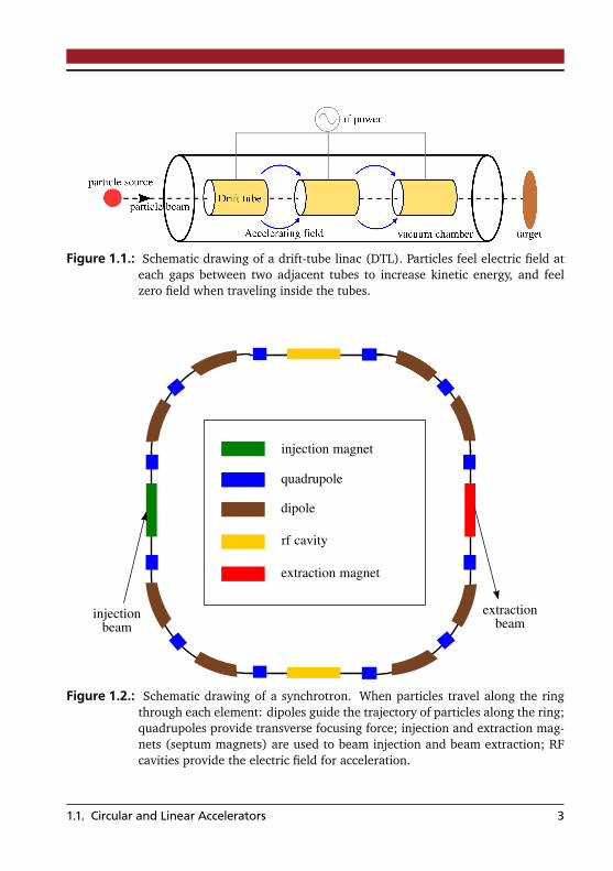
Figure 1.1.: Schematic drawing of a drift-tube linac (DTL). Particles feel electric field ateach gaps between two adjacent tubes to increase kinetic energy, and feelzero field when traveling inside the tubes.
injection magnet
quadrupole
dipole
rf cavity
extraction magnet
extractionbeam
injectionbeam
Figure 1.2.: Schematic drawing of a synchrotron. When particles travel along the ringthrough each element: dipoles guide the trajectory of particles along the ring;quadrupoles provide transverse focusing force; injection and extraction mag-nets (septum magnets) are used to beam injection and beam extraction; RFcavities provide the electric field for acceleration.
1.1. Circular and Linear Accelerators 3

SIS-100/300
Super-FRSHESR
NESRCR/RESR
SIS-18p-linac
UNILAC
CBM
PANDA
FLAIR
Plasma and atomic physics
Antiproton production target
Rare isotope production target
Figure 1.3.: Layout of the FAIR project. Ion beams generated at ion source (at the startpoint of UNILAC) are accelerated via UNILAC to 11.4 MeV/u, and injectedto booster synchrotron SIS-18, where the typical kinetic energy of particlesare at the range of 200 MeV/u to 4 GeV/u. Those particles are transported toSIS-100 for further acceleration, where the final kinetic energy of particles canreach up to 28 GeV/u (for protons). Particles can be extracted from SIS-100for various experiments.(figure from [3])
1.2 FAIR Project at GSI
The GSI Helmholtzzentrum für Schwerionenforschung (Helmholtz center for heavy ionresearch) [10] is a worldwide unique large-scale accelerator facility for fundamentalresearch with ion beams. It was set-up in 1969 and is jointly funded by the FederalRepublic of Germany and the state of Hessen. As an international state-of-the-art, mul-tipurpose accelerator complex in Europe, FAIR is currently under construction at GSI incooperation of an international community of countries and scientists. FAIR will consistof ion synchrotron; the upgraded SIS-18, the SIS-100 and several storage rings as wellas beam targets. The layout of the accelerator and experiment of FAIR are shown inFig. 1.3.
4 1. Introduction

1.3 Space Charge and Dispersion
Space charge and dispersion are two basic phenomena that affect high-intensity beamdynamics in circular accelerators. In accelerator physics, space charge refers to the elec-tric field created by the Coulomb forces between the charged particles of a beam, partlycancelled by the magnetic field generated from the moving beam. For a beam with anarbitrary charged particle distribution, the joint forces from electric and magnetic fields(space-charge forces) is likely to be nonlinear. In 1959, Kapchinsky and Vladimirskygave an ellipsoid beam distribution that generates a perfect linear space-charge forcein the beam [11]. In this distribution, particles are random-uniformly distributed onboth phase space and real space. This distribution (usually called K-V distribution inthe literature) allows one to study space charge effects in a self-consistent manner be-cause the distribution remains uniform during beam transporting. In most practicalbeams, however, the particle distribution is Gaussian-like, which generates nonlinearspace-charge forces. In order to analyze a realistic particle distribution, Lapostolle andSacherer in 1971 introduced the concept of equivalent beams [12, 13] and the rms enve-lope equations, which describe self-consistently the motion of non-K-V beams with spacecharge in a rms sense. Based on the rms envelope approach, improvements have beenmade on the understanding of the space charge dynamics in the past few decades: theparticle core resonance; beam halo formation [14, 15]; the envelope oscillation and itsinstability [16, 17, 18, 19, 20, 21, 22]; high order beam collective modes and their in-stabilities [1, 23, 24]; and the space charge structural resonance [25, 26]. Recently withthe successful experimental observations of fourfold structure and coupling emittance inhigh-intensity linear accelerators [27, 28], space-charge-driven particle resonance andbeam instability have received renewed interest, since it represents a major intensitylimitation not only in linacs, but also in circular machines.
Dispersion in accelerator physics is analogue to the optical dispersion, where a par-ticle of higher momentum (or energy) is deflected through a lesser angle in a bendingmagnet. For a practical beam with momentum spread (or energy spread), the transversebeam size will enlarge as it passes through a bending magnet. The dispersion effect canbe described quantitatively by the dispersion function, which is one of the most essentialcharacteristics of a circular accelerator.
In recent years, with increasing demand of transporting high-intensity beams in circu-lar accelerators, progress has been made on the study of the influences of space chargeand dispersion on beam dynamics in circular accelerators. In 1998, Marco Venturiniand Martin Reiser developed an envelope equation system with an generalized in-variant emittance in the presence of both dispersion and space charge [29, 30]. Inthe same year, S. Y. Lee and H. Okamoto gave a Hamiltonian expression with a modi-fied dispersion formula including higher order space charge potential terms [2]. Othermethods involve a smooth approximation approach [31] or a modified particle-coremodel [32, 33, 34].
1.3. Space Charge and Dispersion 5

length
energy spread
Figure 1.4.: Bunch compression by fast bunch rotation. The bunch in the horizontal posi-tion is rotated by 90 into an upright position.
1.4 Bunch Compression in Synchrotrons
In many accelerator-based facilities, short and intense ion or proton bunched beams(bunches for short) are required for various applications, such as the production andsubsequent storage of exotic nuclei or antiprotons, generation of dense plasmas andspallation neutron sources. For instance, in both of the synchrotrons SIS-18 and SIS-100at FAIR, short bunches are planned to be achieved via bunch compression process beforeextraction. During bunch compression, as the bunch is compressed, the beam current isincreasing. The resulting space charge effect is enhanced and represents an importantlimitation for the maximum compression ratio as it leads to particle resonance and beaminstability. Therefore, bunch compression must be completed as fast as possible in orderto minimize the dwelling time of bunches in the extreme space charge regime.
A widely-accepted scheme to achieve bunch compression is a 90 non-adiabatic fastbunch rotation in longitudinal phase space due to a ramped high RF voltage. For in-stance, such a fast bunch rotation process is performed before extraction in the SIS-18 [35, 36], and proposed for the FAIR SIS-100 [37]. Fig. 1.4 shows a sketch of the fastbunch rotation. The bunch is rotated via 90 in the longitudinal phase space, decreas-ing the bunch length, at the cost of the energy spread increasing. The enlarged energyspread in the bunch is in inverse proportion to the reduced bunch length due to the in-variant longitudinal emittance 3, and results in an enhanced effect of dispersion. In thepast few years, the scheme of bunch compression based on fast rotation has been thesubject of numerous theoretical studies investigating beam instability limits and beamquality evolution [38, 39, 40, 41, 42, 43, 44, 45, 46, 47].
3 The “longitudinal emittance” refers to the area of the ellipse in Fig. 1.4. For more details seeChapter 2 and Chapter 7.
6 1. Introduction
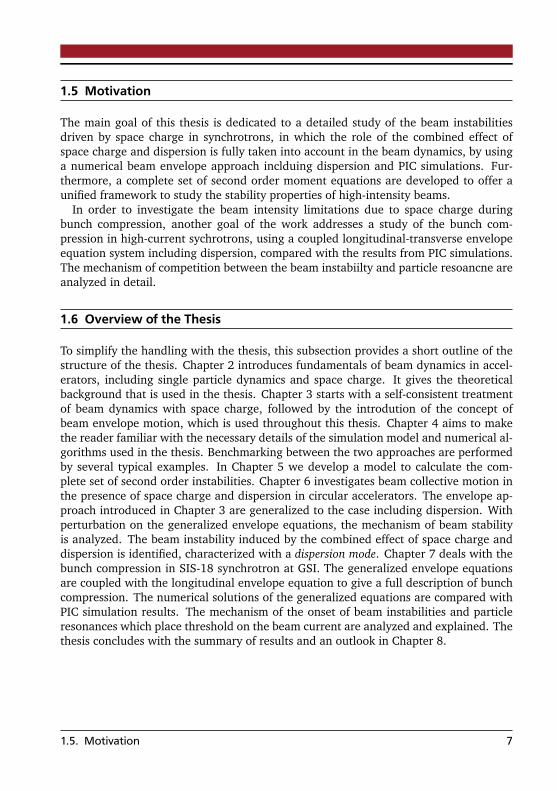
1.5 Motivation
The main goal of this thesis is dedicated to a detailed study of the beam instabilitiesdriven by space charge in synchrotrons, in which the role of the combined effect ofspace charge and dispersion is fully taken into account in the beam dynamics, by usinga numerical beam envelope approach inclduing dispersion and PIC simulations. Fur-thermore, a complete set of second order moment equations are developed to offer aunified framework to study the stability properties of high-intensity beams.
In order to investigate the beam intensity limitations due to space charge duringbunch compression, another goal of the work addresses a study of the bunch com-pression in high-current sychrotrons, using a coupled longitudinal-transverse envelopeequation system including dispersion, compared with the results from PIC simulations.The mechanism of competition between the beam instabiilty and particle resoancne areanalyzed in detail.
1.6 Overview of the Thesis
To simplify the handling with the thesis, this subsection provides a short outline of thestructure of the thesis. Chapter 2 introduces fundamentals of beam dynamics in accel-erators, including single particle dynamics and space charge. It gives the theoreticalbackground that is used in the thesis. Chapter 3 starts with a self-consistent treatmentof beam dynamics with space charge, followed by the introdution of the concept ofbeam envelope motion, which is used throughout this thesis. Chapter 4 aims to makethe reader familiar with the necessary details of the simulation model and numerical al-gorithms used in the thesis. Benchmarking between the two approaches are performedby several typical examples. In Chapter 5 we develop a model to calculate the com-plete set of second order instabilities. Chapter 6 investigates beam collective motion inthe presence of space charge and dispersion in circular accelerators. The envelope ap-proach introduced in Chapter 3 are generalized to the case including dispersion. Withperturbation on the generalized envelope equations, the mechanism of beam stabilityis analyzed. The beam instability induced by the combined effect of space charge anddispersion is identified, characterized with a dispersion mode. Chapter 7 deals with thebunch compression in SIS-18 synchrotron at GSI. The generalized envelope equationsare coupled with the longitudinal envelope equation to give a full description of bunchcompression. The numerical solutions of the generalized equations are compared withPIC simulation results. The mechanism of the onset of beam instabilities and particleresonances which place threshold on the beam current are analyzed and explained. Thethesis concludes with the summary of results and an outlook in Chapter 8.
1.5. Motivation 7

8 1. Introduction

2 Single Particle DynamicsBeam dynamics is main theoretical essence of accelerator physics. The framework ofbeam dynamics evolves from the concepts of classical mechanics, electrodynamics,statistical physics and plasma physics. It aims to describe the behavior of a charged-particle beam traveling in an accelerator and used in accelerator design, operation, andoptimization. In this chapter, we introduce the fundamentals of beam dynamics - thedynamcis of single particle - to the extent needed as a basis for the following chapters.In the framework of single particle dynamcis, we focus on the motion of individualparticles. The collective motion of a beam will be discussed in the next chapter.
Section 2.1 starts with the Hamiltonian of a charged particle in electromagnetic field,to arrive at the equations of transverse motion. Main essential physical quantities, suchas lattice functions, betatron tune, and transverse emittance are briefly presented. Sec-tion 2.2 introduces the concept of dispersion and the dispersion function, which will befurther discussed in the following chapters. Section 2.3 focuses on longitudinal particledynamics. The equaitons of longitudinal motion is derived governed by a longitudinalHamiltonian. Section 2.4 discusses the basic theory of space charge, including both ofthe transverse and longitudinal components.
2.1 Transverse Particle Dynamics
2.1.1 Equations of Motion
A charged particle in electromagnetic field is governed by the Lorentz force [48]
~F =d~pd t= q(~E + ~v × ~B), (2.1)
where q is the charge of the particle, ~v is the velocity of the particle, ~p = γm ~v is theparticle momentum, with γ = (1− v 2/c2)−
12 the relativistic factor, c the speed of light,
and ~E and ~B are respectively the electric field and magnetic field. The ~E and ~B fieldsfollow the Maxwell equations [48]
~E = −∇Φ−∂ ~A∂ t
,
~B =∇× ~A,(2.2)
9

r0
r
reference orbit
ex
ey
es
o
Figure 2.1.: Curvilinear coordinate system for particle motion in circular accelerators.
where, Φ and ~A are the scalar potential and vector potential, respectively. The Lorentzforce in Eq. 2.1 can be derived from the Hamiltonian for particle motion (see, for exam-ple, in [49])
H1 = c[m2c2 + (~P − q~A)2]12 + qΦ, (2.3)
in which ~P = ~p+ q~A is the canonical momentum.
In beam dynamics, it is convenient to adopt a curvilinear coordinate system for parti-cle motion. As shown in Fig. 2.1, ~r denotes the reference orbit, and ~ex , ~ey , and ~es formthe basis of the curvilinear coordinate system, in which ~ex and ~ey form the transverseplane, and ~es represents the longitudinal direction. Any particle’s trajectory around thereference orbit can be expressed as ~r(s) = ~r0(s) + x~ex + y~ey , with (x , y, s), the particlecoordinates in the curvilinear system.
After establishing the curvilinear coordinate system, two steps of derivations areneeded to obtain the equations of particle transverse motion in this coordinate sys-tem. At first, a Hamiltonian of particle motion H2, in term of (x , y, s), with the cor-responding conjugate coordinates (px , py , ps) can be found by performing a canonicaltransformation from the Hamiltonian H1 in Eq. 2.3
H2 = qΦ+ c[m2c2 +(ps − qAs)2
(1+ x/%)2+ (px − qAx )
2 + (py − qAy)2], (2.4)
in which, % is the radius of curvature of the curvilinear system, and the subscripts x , y,and s represent respectively the components in ~ex , ~ey and ~es directions in the curvilinearcoordinate system. Secondly, since in accelerators the scalar and vector potential Φ and
10 2. Single Particle Dynamics

~A are constant1, the longitudinal momentum ps can be chosen as a new Hamiltonian,which can be written as [50]
H3 = −p(1+x%) +
1+ x/%2p
[(px − qAx )2 + (py − qAy)
2]− qAs. (2.5)
Here, we use the approximation that the transverse momenta px and py are muchsmaller than ps.
The transverse equations of motion of a charged particle in the curvilinear coordinatesystem can be derived from the expression of the Hamiltonian H3
d2 xds2−% + x%2
= ±By
B%p0
p
1+x%
2,
d2 yds2
= ∓Bx
B%p0
p
1+x%
2,
(2.6)
in which, p and p0 are the momenta of the particle and the reference particle, respec-tively. Bx = −
∂ As∂ y and By =
∂ As∂ x are the transverse components of the magnetic fields.
B% = p0/q is the magnetic rigidity, defining the energy of the reference particle. A ref-erence particle is chosen in such a way that it travels ideally through the center of themagnets (quadrupoles, dipoles and so on) with its coordinate (x = 0, y = 0) along thereference orbit of the ring. After one complete turn the reference particle will remainon its trajectory and return its initial position. The one periodicity-turn trajectory ofthe reference particle is defined as a closed orbit. Eqs. 2.6 describes the motion of theparticles with their coordinates (x 6= 0, y 6= 0) moving around the closed orbit, which iscalled transverse betatron motion. We solve Eqs. 2.6 without energy spread (i.e., p = p0
) in this section. The case with energy spread (i.e., p 6= p0), which brings the dispersioneffect, will be discussed in next section.
Since the transverse amplitude of betatron motion (x , y) is small, we can linearizeEqs. 2.6 and obtain the Hill equations [51]
d2 xds2+κ0,x (s)x = 0,
d2 yds2+κ0,y(s)y = 0,
(2.7)
where κ0,y = 1/%2 − B1(s)/B%, κ0,y = B1(s)/B% are the effective focusing functions, and
B1 =∂ By∂ x = −
∂ Bx∂ y the quadrupole gradient function evaluated at the closed orbit. Be-
cause of the periodic property of synchrotrons, κ0,x and κ0,y are periodic functions of s,κ0y,0x (s) = κ0x ,0y(s + L) with the periodic length L. Most synchrotrons have separated
1 For most elements in accelerators except the RF cavity, we have ϕ = 0. The non-zero elec-tric potential ϕ plays a key role in the longitudinal motion of particles; magnetic elements inaccelerators usually have transverse magnetic fields with Ax = Ay = 0
2.1. Transverse Particle Dynamics 11

dipoles and quadrupoles for guiding/bending and alternating focusing particles, respec-tively. In a quadrupole where 1/% → 0, we have κ0,x = −κ0,y = B1(s)/B%, indicatingparticles focus in one direction (for example in x-direction) and defocus in another di-rection (for example in y-direction). In a dipole, which usually lies on the xs-plane, wehave κ0,x = 1/% and κ0,y = 0. In addition to guiding the direction of particles, dipolesalso have weak focusing effects since 1/% > 0.
2.1.2 Twiss Parameters
Now let us consider the solution of the Hill equations in Eqs. 2.7. With the periodiccondition, the Hill equations in Eqs. 2.7 are second order homogeneous differentialequations with periodic varying coefficients, and can be solved using Floquet theo-rem [52]. For simplicity, we use the notation z to denote either x or y in transverseplane. The Hill equations in Eqs. 2.7 can be rewritten as2
d2zds2+κ0,z(s)z = 0. (2.8)
After some standard derivations and transformations in textbooks (see, e.g., Ref. [50]),the solution of Eq. 2.8 is
z =q
εzβ0,z(s) cos[k0,z(s) +ϕ0],
z′ =dzds= −
√
√ εz
β0,z(s)
α0,z(s) cos[k0,z(s) +ϕ0] + sin[k0,z(s) +ϕ0]
.(2.9)
Here, β0,z(s) is the betatron amplitude function, or beta function. The motion that aparticle performs described in Eqs. 2.9 is called betatron motion. α0,z(s) is the negativeslope of β0,z(s)with α0,z(s) = −β ′0,z(s)/2. The functions β0,z(s), α0,z(s), along with anotherquantity defined by γ0,z = (1+ α2
0,z)/β0,z are called the Courant-Snyder parameters, orTwiss parameters, which characterize the fundamental properties of the sequences of themagnets (lattice) in accelerators. The quantity εz is the single particle emittance, whichis a constant of integration and will be discussed in detail in the next subsection. ϕ0 inEqs. 2.9 is the initial phase advance and usually chosen as zero for simplicity. k0,z(s) isthe betatron phase advance (or phase advance for short) in the z-dirction that a particleachieves after performing beatron motion on a length of s, and can be calculated byintegrating the beta function over the length
k0,z(s) =
∫ s
0
dsβ0,z(s)
. (2.10)
2 Here, we use the subscript ‘0’ in the κ and the quantities in the following to denote the quantitiesfor accelerators, which are independent of the beam.
12 2. Single Particle Dynamics

Consider a circular accelerator with its circumference of C = nL, where n is the numberof periodic structures of the accelerator and L is the length of one period. After onerevolution, the betatron phase advance (in the z-direction) that a particle achieves is
kC =
∫ nL
0
dsβ0,z(s)
, (2.11)
The number of betatron oscillations per revolution, also known as the betatron tunealong the z-direction defined as
Q0,z =kC
2π=
12π
∫ nL
0
dsβ0,z(s)
. (2.12)
In a beam, individual particles in betatron oscillation have individual tunes. The tuneof a reference particle, is called a working point, and is important for accelerator designand operation since the particle resonance is usually related to the choices of tunes. Forexample, for a circular accelerator with an integer Q0,z , particles return to each locationin the accelerator with the same betatron phase, since the betatron phase advnace perpassage is an integer multiple of 2π. We assume a small imperfection of dipole magnetsexists at the position of s0, particles experience a slight change of its coordinate due tothe magnetic error at s0 per passage. Upon subsequent passes, the change accumulatesin phase and resulting in resonance, leading to the amplitude growth and particle loss3.
With the Twiss parameters and phase advance in Eq. 2.9 and Eq. 2.10, the transversebetatron motion of Eq. 2.8 can be described in matrix form as
M(s2|s1) = B(s2)
cos k0,z sin k0,z
− sin k0,z cos k0,z
B−1(s1), (2.13)
with
B(s) =
Æ
β0,z(s) 0
− α0,z (s)pβ0,z (s)
1pβ0,z (s)
!
. (2.14)
The matrix M(s2|s1) is called the transfer matrix and characterizes particle betatronmotion from s1 to s2 by
z(s2) =M(s2|s1)z(s1), (2.15)
where z = (z, z′)T is the vector of transverse particle coordinates. Eq. 2.15 is widelyused for solving the equation of betatron motion, as well as for particle tracking insimulations.
3 Besides driven by the external magnetic imperfections of accelerator elements described here,particle resonance can also be driven by the electromagnetic field (space charge) of the beamitself, which will be discussed in Chapter 3.
2.1. Transverse Particle Dynamics 13

o
Figure 2.2.: Single particle emittance in z-direction: the invariant of a particle betatronmotion in (z, z′) phase space. The elliptical area enclosed is equal to πεz .The maximum amplitude of betatron motion is
Æ
β0,zεz and the maximumdivergence angle is
p
γ0,zεz .
2.1.3 Emittance
Another essential quantity in beam dynamics is the emittance, as introduced in Eqs. 2.9.To show the physical meaning of the emittance, we combine the two equations in Eq. 2.9and obtain
εz = γ20,zz
2 + 2α0,zzz′ + β0,zz′2, (2.16)
which defines an ellipse in the phase space (z, z′), characterizing the trajectory of thebetatron motion of a particle after traveling one periodic structure, as shown in Fig 2.2.The emittance of a single particle is determined by the initial coordinate of the particle,and independent of the external focusing strengths. Particles with different initial coor-dinates (z0, z′0) have different emittances; however the emittance of each particle is aninvariant as it is transported in an accelerator.
While the emittance defined in Eq. 2.16 characterizes the motion of single particle, tocharacterize the whole beam, the maximum single particle emittance is defined as theemittance of the beam,
εz = εz,max . (2.17)
In the z − z′ phase space, different single particle emittances define a series of concen-tration ellipse. The beam emittance εz defines the largest concentration ellipse. The
14 2. Single Particle Dynamics
motion of the particles is associated with an equivalent motion of the correspondingpoints on each concentration ellipse. In most cases in accelerators, a beam can beassumed as a system of non-interacting particles. While accelerators consist of bothof linear and nonlinear elements, for beam motion, the linear elements (i.e., focusingand guiding/bending) are the dominant component. According to Liouville’s theorem,which states that the volume occupied by a given number of particles in phase spaceremains invariant with time, the emittance of a beam is constant during transport in ac-celerators. In the following chapters, the invariance of the emittance will be generalizedto include electromagnetic interactions between charged particles.
2.2 Dispersion Function
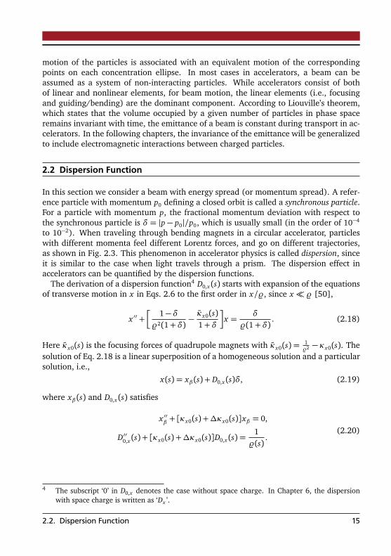
In this section we consider a beam with energy spread (or momentum spread). A refer-ence particle with momentum p0 defining a closed orbit is called a synchronous particle.For a particle with momentum p, the fractional momentum deviation with respect tothe synchronous particle is δ = |p − p0|/p0, which is usually small (in the order of 10−4
to 10−2). When traveling through bending magnets in a circular accelerator, particleswith different momenta feel different Lorentz forces, and go on different trajectories,as shown in Fig. 2.3. This phenomenon in accelerator physics is called dispersion, sinceit is similar to the case when light travels through a prism. The dispersion effect inaccelerators can be quantified by the dispersion functions.
The derivation of a dispersion function4 D0,x (s) starts with expansion of the equationsof transverse motion in x in Eqs. 2.6 to the first order in x/%, since x % [50],
x ′′ +
1−δ%2(1+δ)
−κx0(s)1+δ
x =δ
%(1+δ). (2.18)
Here κx0(s) is the focusing forces of quadrupole magnets with κx0(s) =1%2 − κx0(s). The
solution of Eq. 2.18 is a linear superposition of a homogeneous solution and a particularsolution, i.e.,
x(s) = xβ (s) + D0,x (s)δ, (2.19)
where xβ (s) and D0,x (s) satisfies
x ′′β+ [κx0(s) +∆κx0(s)]xβ = 0,
D′′0,x (s) + [κx0(s) +∆κx0(s)]D0,x (s) =1%(s)
.(2.20)
4 The subscript ‘0’ in D0,x denotes the case without space charge. In Chapter 6, the dispersionwith space charge is written as ‘Dx ’.
2.2. Dispersion Function 15
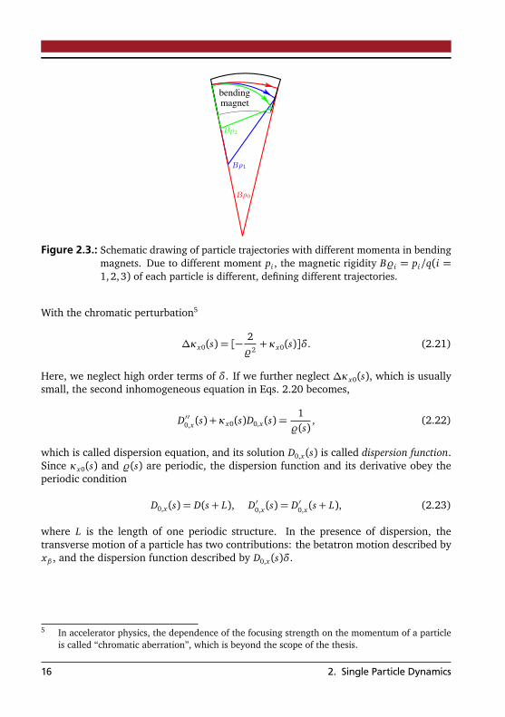
bendingmagnet
Figure 2.3.: Schematic drawing of particle trajectories with different momenta in bendingmagnets. Due to different moment pi , the magnetic rigidity B%i = pi/q(i =1, 2,3) of each particle is different, defining different trajectories.
With the chromatic perturbation5
∆κx0(s) = [−2%2+κx0(s)]δ. (2.21)
Here, we neglect high order terms of δ. If we further neglect ∆κx0(s), which is usuallysmall, the second inhomogeneous equation in Eqs. 2.20 becomes,
D′′0,x (s) + κx0(s)D0,x (s) =1%(s)
, (2.22)
which is called dispersion equation, and its solution D0,x (s) is called dispersion function.Since κx0(s) and %(s) are periodic, the dispersion function and its derivative obey theperiodic condition
D0,x (s) = D(s+ L), D′0,x (s) = D′0,x (s+ L), (2.23)
where L is the length of one periodic structure. In the presence of dispersion, thetransverse motion of a particle has two contributions: the betatron motion described byxβ , and the dispersion function described by D0,x (s)δ.
5 In accelerator physics, the dependence of the focusing strength on the momentum of a particleis called “chromatic aberration”, which is beyond the scope of the thesis.
16 2. Single Particle Dynamics

The solution of Eqs. 2.20 can be written in matrix form as
D(s2)D′(s2)
1
=
M(s2|s1) d0 1
D(s1)D′(s1)
1
, (2.24)
with particular solution
d =
1%κx0(1− cos
pκx0s)
1%pκx0
sinpκx0s
if κx0 ≥ 0,
1%|κx0 |
(coshp
|κx0|s− 1)1
%p|κx0 |
sinhp
|κx0|s
if κx0 < 0.
(2.25)
Here, M(s2|s1) is the 2×2 transfer matrix introduced in Eq. 2.13, % is the dipole bendingradius, and κx0 is the effective focusing force of quadrupole magnets (usually piecewiseconstant). With the initial condition D(s1) and D′(s1) at the initial position s = s1,the dispersion function D(s2) and its derivative D′(s2) at s = s2 can be obtained fromEq. 2.24. Moreover, with the periodic condition of Eqs. 2.23 imposed on Eq. 2.24, thedispersion function in a periodic structure can be calculated without any initial particlecoordinates.
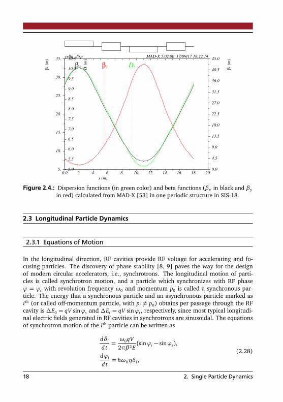
Conceptually, dispersion is to quantitatively characterize the coupling effect of thelongitudinal beam energy spread and the transverse betatron motion. Dispersion func-tions, along with Twiss parameters, provide the quantitative basis for describing accel-erator properties, and are essential for accelerator design and operation. Fig. 2.4 showsan example of dispersion functions and beta functions in one periodic structure in thesynchrotron SIS-18 at GSI.
In the presence of dispersion, particles with different momenta travel on differentclosed orbits. To evaluate the total length difference of the closed orbit between parti-cles, the concept of momentum compaction factor is introduced, as
αc =1C
∮
D(s)%
ds, (2.26)
in which C is the circumference. The phase-slip factor can be defined as η = αc −1γ2 ,
connecting the revolution period with the momentum offset by
∆ω
ω0= −η
∆TT0
. (2.27)
Eq. 2.27 indicates that the shift of revolution frequency affects the longitudinal motionof particles, which will be discussed in the next subsection.
2.2. Dispersion Function 17
0.0 2. 4. 6. 8. 10. 12. 14. 16. 18. 20.
s (m)
cella_disp MAD-X 5.02.00 17/09/17 18.22.14
5.
10.
15.
20.
25.
30.
35.
βx(m
)
0.0
4.5
9.0
13.5
18.0
22.5
27.0
31.5
36.0
40.5
45.0
βy
(m)
5.0
5.5
6.0
6.5
7.0
7.5
8.0
8.5
9.0
9.5
10.0
10.5
Dx
(m)
β x β y Dx
Figure 2.4.: Dispersion functions (in green color) and beta functions (βx in black and βyin red) calculated from MAD-X [53] in one periodic structure in SIS-18.
2.3 Longitudinal Particle Dynamics
2.3.1 Equations of Motion
In the longitudinal direction, RF cavities provide RF voltage for accelerating and fo-cusing particles. The discovery of phase stability [8, 9] paves the way for the designof modern circular accelerators, i.e., synchrotrons. The longitudinal motion of parti-cles is called synchrotron motion, and a particle which synchronizes with RF phaseϕ = ϕs with revolution frequency ω0 and momentum p0 is called a synchronous par-ticle. The energy that a synchronous particle and an asynchronous particle marked asith (or called off-momentum particle, with pi 6= p0) obtains per passage through the RFcavity is ∆E0 = qV sinϕs and ∆Ei = qV sinϕi , respectively, since most typical longitudi-nal electric fields generated in RF cavities in synchrotrons are sinusoidal. The equationsof synchrotron motion of the ith particle can be written as
dδi
d t=ω0qV2πβ2E
(sinϕi − sinϕs),
dϕi
d t= hω0ηδi ,
(2.28)
18 2. Single Particle Dynamics

in which δi = (pi − p0)/p0 is the fractional momentum deviation, V is the RF voltage, his the harmonic number of the RF system, ϕi and ϕs are respectively the phase of theith particle and the synchronous particle with respect to the RF wave6, ω0, β and E arethe angular velocity, linear velocity and the total energy of the synchronous particle,respectively. The first equation in Eqs. 2.28 is the equation of motion for the “energydifference" and the second one in Eqs. 2.28 is the phase equation. Eqs. 2.28 indicatethat an asynchronous particle oscillates around the synchronous particle.
Equations 2.28 can be derived mathematically from a longitudinal Hamiltonian of theith particle, with (δ,ϕ) as the phase space coordinates
HL =12
hω0ηδ2i +
ω0qV2πβ2E
[cosϕi − cosϕs + (ϕi −ϕs) sinϕs], (2.29)
in which the first term is “kinetic energy” and the second term is “potential energy”.The synchrotron frequency for small amplitude synchrotron oscillation can be obtainedfrom the Hamiltonian linearizion7,
ωs =cR
√
√hqV |η cosϕs|2πE
, (2.30)
where c is the speed of light and R the average radius of the synchrotron. The syn-chrotron tune, defined as the number of synchrotron oscillations per revolution, can beobtained from Eq. 2.30
Qs =ωs
ω0=
√
√hqV |η cosϕs|2πβ2E
. (2.31)
For ion or proton accelerators, typically the longitudinal beam length is much longerthan transverse beam size, and Qs is of the order of 10−3, which is much smaller thanthe transverse betatron tune.
2.3.2 Bucket and Longitudinal Emittance
The nonlinear Hamiltonian in Eq. 2.29 defines the particle trajectories in the longitu-dinal phase space. The synchronous particle is located at the stable fixed point (ϕs, 0),and performs no synchrotron oscillation. The trajectories of off-momentum particlesperform synchrotron oscillations around the stable fixed point. For small amplitudes,
6 In many literatures, ϕs is named as synchronous phase.7 For small amplitude, the linearized Hamiltonian is HL =
12 hω0ηδ
2i −
ω0qV cosϕs4πβ2 E ϕ2
i .
2.3. Longitudinal Particle Dynamics 19

−150 −100 −50 0 50 100 150
φ (deg)
−1.5
−1.0
−0.5
0.0
0.5
1.0
1.5δ s
x
√πβ2Eh|η|/e
Vφs = 0
φs = 30
φs = 60
Figure 2.5.: The separatrix with ϕs = 0, 30, 60. The separatrix area decreases with ϕsincreases.
the trajectories become ellipses8. The largest trajectory can be found by the unstablefixed point (ϕ = π−ϕs,δ = 0)
Hsx =ω0qV2πβ2E
[−2cosϕs + (π− 2ϕs) sinϕs], (2.32)
which is called separatrix. The enclosed area of the separatrix is called the bucket. Thebucket with ϕs = 0 has the largest area, as shown in Fig. 2.5 in blue curve. With a givenRF voltage, the bucket area will shrink as ϕs increases. With a given ϕs, the bucketheight is inversely proportional to the RF voltage.
Similar to the case in transverse phase space, the enclosed area of the particle tra-jectory in longitudinal phase space is called longitudinal emittance. With the smallamplitude approximation, the longitudinal emittance can be written as the area of theellipse εL = πδϕ, which is constant in the absence of acceleration.
2.4 Basic Theory of Space Charge
The framework of single particle dynamics that have been discussed so far are the in-vestigation of the motion of an individual particle under the external electromagneticfield of various components (e.g., magnets and RF cavities) in accelerators. This pic-ture holds well for particles in a beam with low intensity. For high-intensity beams,it no longer applies, since the interaction between charged particles, or the interac-tion between the beam and the its surroundings (for example, the beam vacuum pipe,
8 This can be shown by the linearized Hamiltonian HL .
20 2. Single Particle Dynamics

beam diagnostics and so on) has to be taken into account. The former interactionis called direct space charge or space charge, and the later is called the indirect spacecharge or impedance. In fact, coulomb forces exist between charged particles, increasingfrom zero at beam center towards the edge, and push particles away from beam cen-ter. Meanwhile, as charged particles move along the path in an accelerator as a beamcurrent, a magnetic field is generated between particles, which partially cancels theelectrostatic defocusing effect of Coulomb forces. The combined effect of electrostaticdefocusing and magnetic focusing, which is still repulsive, is the effect of space chargeor self fields inside the beam [54]. On the other hand, the beam interacts electromagnet-ically with its surroundings, and can be treated as an impedance [55], which is beyondthe scope of this thesis. Space charge is the most basic collective effect of charged par-ticle beams. In principle, the treatment of space charge is a three-dimensional (3-D)problem. However, for most synchrotrons with proton or ion beams, the length of beamis usually much longer than the transverse width and the space charge coupling be-tween transverse and longitduain direction can be neglected, thus the space charge canbe decomposed into transverse and longitudinal components.
This section focuses on the fundamentals of space charge. In the following of thissection, we will firsty introduce the transverse space charge, and secondly discuss brieflythe longitudinal space charge.
2.4.1 Transverse Space Charge
Following the standard description of transverse space charge (see, for example, inRef. [56]), we first consider the space charge in the case of an unbunched beam, orcoasting beam with a round cross-section and uniform charge density traveling in aperfectly conducting round beam pipe with a constant longitudinal velocity. We assumethat the radius of the beam pipe is much larger than the radius of the beam, so that theimage charge phenomenon can be neglected. Such a coasting beam can be modeled asa “beam cylinder” with infinite length, as shown in Fig. 2.6.
To calculate electric and magnetic fields E and B generated by the coasting beam, wechoose a small cylinder inside the beam with radius r and length l, as shown in reddashed lines in Fig. 2.6. According to Gauss’ law, in the cylindrical coordinate systemwe have
∫∫∫
V
∇ · EdV =
∫∫∫
V
η
ε0dV =
S
E · dS, (2.33)
in which η is the uniform charge density in the unit of [C b/m3], dV represents an unitvolume inside the cylinder, and dS an unit of its surface. With integrals over the closedsurface and the volume of the small cylinder, we obtain
Er =I
2πε0β cra2
. (2.34)
2.4. Basic Theory of Space Charge 21

beam pipe
beam
Figure 2.6.: Schematic drawing of the distribution of electromagnetic fields in the beamcylinder model. The upper plot (a) shows the electromagnetic fields on theprofile of the beam cylinder; and the lower plot (b) shows the electromagneticfields in the cross section of the beam cylinder.
22 2. Single Particle Dynamics

Here, I is the beam current, β c the speed of beam, with c the speed of light in vacuum,ε0 is the vacuum permittivity. Similarly, the magnetic field B can be found by Stokes’law,
∫∫
∇×B · dS=
∫∫
µ0J · dS=
∮
S
Bds, (2.35)
where µ0 is the vacuum permeability, J = qβ c is the current density with q the chargeof the individual particle. With integrals over the small cylinder of radius r and lengthl, Eq. 2.35 yields
Bϑ =I
2πε0c2
ra2
. (2.36)
It can be seen that the transverse symmetry of the beam cylinder lead to the radialelectric field Er and azimuthal magnetic field Bϑ. The Lorentz force from beam self fieldacting on a particle can be found from Eq. 2.34 and Eq. 2.36
Fr = qEr − qβ cBϑ =qI
2πε0β cγ2
ra2
, (2.37)
which is linear and radial. The first part qEr denotes the repulsive electrostatic force,which is independent with beam velocity, and the second part −qβ cBϑ denotes themagnetic force, which is attractive and increasing with beam velocity. The overall effectof the two parts is repulsive but decrease with beam velocity, with a cancellation factor1/γ2. In the limit case of a beam traveling at the speed of light c, the cancellation factorbecomes zero and the two parts become equal and cancel each other. Replacing r bythe transverse coordinates x , y results in the horizontal and vertical force.
In the following we derive the equation of motion for a charged particle with spacecharge. For simplicity, we take the x-direction (the case in y-direction can be obtainedin a similar way). The space charge force in x-direction has the form:
Fx =qI x
2πε0cβγ2a2. (2.38)
Taking the arc length s in the curvilinear coordinate as the independent variable insteadof time t, we have from Eq. 2.38
x ′′ =d2 xds2
=1β2c2
d2 xd t2
=xβ2c2
=1β2c2
Fx
m0γ=
2r0 Iea2β3γ3c
x , (2.39)
where r0 = q2/(4πε0m0c2) is the classical particle radius with m0 the rest mass of theparticle. In the presence of space charge, the Hill equation of Eq. 2.7 is modified to
x ′′ + [κx0(s)−∆κx (s)]x = 0, (2.40)
2.4. Basic Theory of Space Charge 23

Figure 2.7.: Comparison between the particle distribution (upper plot) and the linecharge density (lower plot) of a coasting beam and a bunched beam.
where ∆κx = 2r0 I/(qa2β3γ3c) is the space charge defocusing term, indicating that thespace charge forces weaken the external focusing forces. Usually, since the beam radiusa varies as beam traveling in accelerators9, the space charge force Fx and space chargedefocusing term ∆κx are also functions of s.
One of the most important consequence of the space charge effect is the space-chargetune shift ∆Qsc: since the space charge leads to defocusing of beams in transverseplane10, particles in a beam will experience a space-charge-depressed tune Qsc withQsc = Q0 −∆Qsc, in which Q0 is the bare betatron tune without space charge. In otherwords, the frequency of transverse betatron oscillation of a particle is depressed due tothe space charge effect. The space-charge tune shift (in x-direction) can be obtained bythe combination of Eq. 2.12 and Eq. 2.40
∆Qsc,x =1
4π
∫ 2πR
0
∆κx (s)βx (s)ds = −1
4π2r0 I
qβ3γ3c
∫ 2πR
0
βx (s)a2
ds. (2.41)
Here, a is the transverse beam size, and βx (s) is the beta function. Several conclusionscan be drawn from Eq. 2.41: (1). The space-charge tune shift is proportional to beamintensity; (2). For electron synchrotrons, in which 1/γ3 ≈ 0, the space-charge tune shiftand space charge effect can be neglected; (3). When beam intensity and energy is given,the space-charge tune shift is inversely proportional to the transverse beam size.
The theory of space charge discussed so far is for coasting beams. For the case ofbunched beams, Eq. 2.34, Eq. 2.36 and Eq. 2.40 still hold, provided that the beam is
9 In alternating gradient channles in accelerators, the radius of the travelling beam is a functionof s because the focusing forces is function of s.
10 The focusing forces of quadrupole magnets felt by a charged particle are partly cancelled bythe defocusing forces of space charge, leading to an effective focusing strength acted on theparticle.
24 2. Single Particle Dynamics
one synchrotron oscillation period
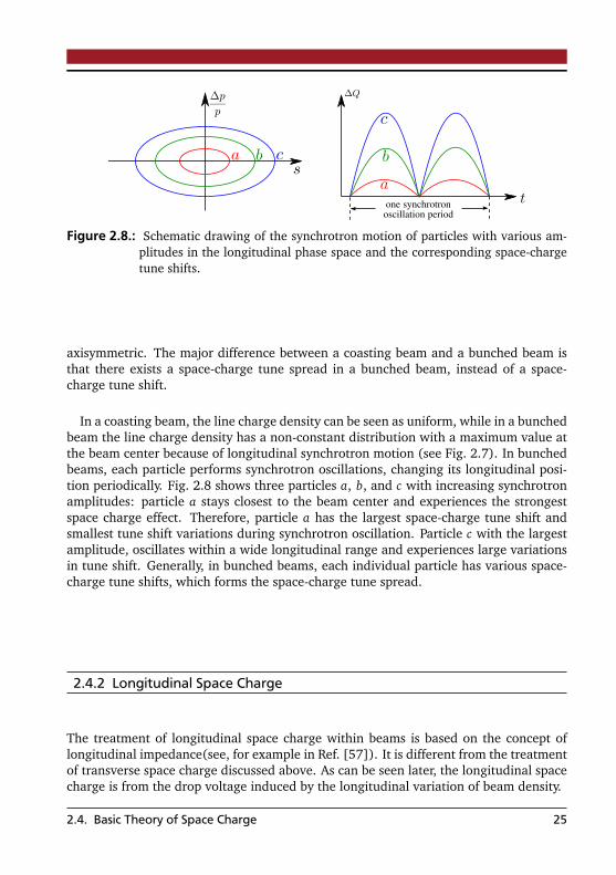
Figure 2.8.: Schematic drawing of the synchrotron motion of particles with various am-plitudes in the longitudinal phase space and the corresponding space-chargetune shifts.
axisymmetric. The major difference between a coasting beam and a bunched beam isthat there exists a space-charge tune spread in a bunched beam, instead of a space-charge tune shift.
In a coasting beam, the line charge density can be seen as uniform, while in a bunchedbeam the line charge density has a non-constant distribution with a maximum value atthe beam center because of longitudinal synchrotron motion (see Fig. 2.7). In bunchedbeams, each particle performs synchrotron oscillations, changing its longitudinal posi-tion periodically. Fig. 2.8 shows three particles a, b, and c with increasing synchrotronamplitudes: particle a stays closest to the beam center and experiences the strongestspace charge effect. Therefore, particle a has the largest space-charge tune shift andsmallest tune shift variations during synchrotron oscillation. Particle c with the largestamplitude, oscillates within a wide longitudinal range and experiences large variationsin tune shift. Generally, in bunched beams, each individual particle has various space-charge tune shifts, which forms the space-charge tune spread.
2.4.2 Longitudinal Space Charge
The treatment of longitudinal space charge within beams is based on the concept oflongitudinal impedance(see, for example in Ref. [57]). It is different from the treatmentof transverse space charge discussed above. As can be seen later, the longitudinal spacecharge is from the drop voltage induced by the longitudinal variation of beam density.
2.4. Basic Theory of Space Charge 25

beam
beam pipe
Figure 2.9.: Schematic drawing of electromagnetic field distribution for a coasting beamwith a beam pipe. EW and Es are caused by impedance. The red dashedrectangular loop is the path integral of Faraday’s law.
For a coasting beam with round cross section traveling inside a round beam pipe, theelectromagnetic fields distributed inside the beam and outside the beam can be writtenas
Er =
qλr2πε0a2
if r ≤ a,
qλ2πε0r
if r > a,
and Bϑ =
µ0qλβ cr2πε0a2
if r ≤ a,
µ0qλβ c2πr
if r > a,
(2.42)
where λ = I/(qβ c) is the line charge density. As shown in Fig. 2.9, the electric field Er
is in radial direction and the magnetic field Bϑ is azimuthal and perpendicular to thepage.
In coasting beams, the line charge density λ is constant. Now we consider a smallperturbation on λ, λ(s) = λ0 +
∂ λ(s)∂ s with ∂ λ(s)
∂ s λ0. The perturbation generates alongitudinal electric filed Ez inside the beam. According to Faraday’s law
∮
~E · d~l = −∂
∂ t
∫
~B · d~S, (2.43)
where d~S is the surface integral. Integrating along the loop marked with the red dashedline in Fig. 2.9, we obtain
∮
~E · d~l = Ez∆z +
∫ b
0
Er(z +∆z)dr + EW (−∆z) +
∫ 0
b
Er(z)dr, (2.44)
26 2. Single Particle Dynamics
where∫ 0
b
Er(z)dr =
∫ a
b
Er(z)dr +
∫ 0
a
Er(z)dr =qg0λ(s)
4πε0, (2.45)
with the geometry factor g0 = 1+ 2 ln b/a. Substituting the above equation to Eq. 2.44,we obtain
∮
~E · d~l = (Ez − EW )∆z +qg0
4πε0[λ(z +∆z)−λ(z)]. (2.46)
Similarly, the surface integral of magnetic field becomes
∫
~B · d~S =
∫ a
0
µ0qλ(s)β cr2πa2
dr +
∫ b
a
µ0qλβ c2πr
dr
∆z =µ0qλ(s)g0β c
4π, (2.47)
and its time derivative is
−dd t
∫
~B · d~S = −∆sµ0qβ cg0
4π∂ λ
∂ t. (2.48)
Combining Eqs. 2.43, 2.46, and 2.48, the longitudinal electric field inside the beam hasthe form
Ez = EW +qg0
4πε0γ2β c∂ λ
∂ s, (2.49)
where the factor 1/γ2 arises from the partial cancellation between the electric and mag-netic fields. EW represents the beam-pipe-induced electric field. By integrating of Ez
along the circumference of accelerator, the total voltage after one turn induced by Ez onthe beam takes the form
∆Usc = −qβ cR∂ λ
∂ s
g0Z0
2βγ2−ω0 L
, (2.50)
where Z0 = 1/ε0c ≈ 377Ω is the vacuum impedance and L is the inductance of the beampipe. Ez in Eq. 2.49 is the longitudinal space charge field, and ∆Usc in Eq. 2.50 is thecorresponding longitudinal space charge voltage.
2.4. Basic Theory of Space Charge 27

28 2. Single Particle Dynamics
3 Fundamentals of Intense BeamDynamics
Charged particle beams, in which the electromagnetic fields (or self field) generated bythe charged particles plays a significant role on the beam dynamics, refers as intensebeams. As an intense beam travelling in an accelerator, the motion of the beam is influ-enced by both the space charge and the external focusing forces of the accelerator. In anintense beam, the self fields change both of the velocity and position of particles, whichare presented as space charge in the previous chapter. It results in variation of chargedensity and particle distribution of the beam. On the other hand, the charge densityand particle distribution are the sources of electromagnetic fields, which, together withexternal forces of accelerator elements, determine the self field and the motion of parti-cles. Thus a self-consistent system forms between the self field and particle distribution(charge density) inside the beam. One deals with a closed loop in which the motion ofthe particle distribution and self fields interrelate and change each other.
In an intense beam travelling in an accelerator, the Coulomb interaction among thecharged particles has an “immediate” collisional effect to the neighbor particles and along range effect on the whole beam. For the physics of plasma point of view, wherecharged-particle beams can be seen as non-neutral plasmas [58], the Debye length formost practical beams for most practical beams is much larger that the average distancebetween two neighbor particles, and the collisional effect is rather small and can beneglected [54]. A widely-accepted method to solve the self-consistency problem ofsuch collisionless-particle system is the Vlasov model [59], in which the Vlasov equa-tion set, is combined with Liouville’s theorm and Maxwell equation set to describe thebeam dynamics in a self-consistent way. The time-independent solutions of Vlasov-Maxwell equation set define the equilibrium states of a particle distribution. To solvethe self-consistent system based on the Vlasov model requires a truly theoretical modelin which the particle distribution follows the closed loop. Up to now, the only knownparticle distribution that follows the closed loop self-consistently in alternating-gradientfocusing accelerators is the Kapchinsky-Vladimirsky distribution or K-V distribution, dis-covered in 1959 [11].
As intense beams in accelerators can be seen as non-neutral plasmas in which colli-sions between particles can be neglected, one can introduce a “space charge potential”to characterize the smoothed effect of space charge acting over the whole beam. Fromthis point of view, the beam as a whole exhibit a collective behavior under the combinedinfluence of external focusing of the accelerator and self field of the beam. To com-pare the collective behaviors of beams with different particle distributions, the conceptof equivalent beam and rms envelope equation was estabilished [12, 13] based on the
29

comparison of the second moments of different particle distributions. The appraochof rms envelope equation provides the information of particle motion in the statisticalsense, and allows one to investigate the beam collective motion self-consistently in anrms sense. For an intense beam cycling in a synchrotron, the length of the beam usuallyis much larger than its transverse width. Therefore, analogy to the treatment of spaccharge, beam motion can be seperated into transverse motion and longitudainl motion.
This chapter is organized as follows. We firstly introduce the K-V distribution in a self-consistent manner in Section 3.1. The envelope model for transverse beam motion areestabilished in Section 3.2. Section 3.3 discusses the beam envelope instabilities. In Sec-tion 3.4, we briefly discuss the longitudinal beam dynamics based on the longitudianlenvelope equation.
3.1 The Kapchinsky-Vladimirsky (K-V) Distribution
The beam with the K-V particle distribution is named as K-V beam. In K-V beams, par-ticles are random-uniformly distributed on the surface of a hyper-ellipsoid in the 4-dimensional phase space, with its elliptical projection in the 2-dimensional phase space.One major property of the K-V distribution is that it creates linear space charge forcesinside the beam. In the following we will briefly give a self-consistent description of K-Vbeams.
We first consider a coasting K-V beam, which has an elliptical cross section and auniform distribution in both x and y. This beam model has a sharp boundary with aconstant beam density % inside the beam, and % = 0 outside the beam, as shown inFig. 3.1. The ellipse describing the boundary of the beam obeys the equation
x2
X 2+
y2
Y 2= 1, (3.1)
and the density is
% =I
πv X Y(3.2)
within the boundary, and % = 0 beyond the boundary. The electric and magnetic fieldsfor such a distribution can be obtained according to the Gauss’s law and the Stokes’slaw1
Ex =I
πε0β cx
X (X + Y ), Ey =
Iπε0β c
yY (X + Y )
, (3.3)
and
Bx =µ0 Iπ
yY (X + Y )
, By =µ0 Iπ
xX (X + Y )
, (3.4)
1 see Eq. 2.33 and Eq. 2.35 in Chapter 2.
30 3. Fundamentals of Intense Beam Dynamics

Figure 3.1.: Schematic drawing of the cross section of a K-V beam, on which particlesdistribute random-uniformly on the ellipse with the semi-major axis X andthe major semi-axis Y .
where I is the beam current, β c is the speed of beam with c the speed of light, ε0 andµ0 are respectively the vacuum permittivity and vacuum permeability. It can be seen inEqs. 3.3 that the electromagnetic fields Ex ,y and Bx ,y a particle feels are in proportion tothe transverse position (x , y) of the particle. In the beam center, Ex ,y = Bx ,y = 0.
The linear space charge forces in x and y can be obtained by Fx = q(Ex + v By) andFy = q(Ey + v Bx ) from Eqs. 3.3 and Eqs. 3.4. In the presence of the linear space charge,the equations of transverse motion for a single particle of Eq. 2.8 in Chapter 2 is modi-fied and takes the form2:
x ′′ + κx x = 0, y ′′ +κy y = 0, (3.5)
with
κx = κx0 −2Ksc
X (X + Y ), κy = κy0 −
2Ksc
Y (X + Y ). (3.6)
Here, κx0,y0 are the external focusing strengths3, κx ,y are the space-charge depressedexternal focusing strengths, Ksc = 2NL rc/(β2γ3) is the space charge perveance, with NL
the number of particles per length, rc the classical particle radius, β and γ the relativisticfactors. Comparing Eqs. 3.5 with Eq. 2.8 indicates that the external focusing forces acted
2 Here, Eqs. 3.5 are for K-V beams. The space-charge-modified Hill equation of Eq. 2.40 in Chapter2 is for a more general coasting beam, independent of particle distributions.
3 In the following, for brevity, we combine the subscripts in the same class of physical quantities.For example, κx0 and κy0 are written as κx0,y0.
3.1. The Kapchinsky-Vladimirsky (K-V) Distribution 31
on particles are depressed by the space charge. Eqs. 3.5 can be solved using a similartreatment of Eq. 2.8
x(s) =Æ
βxεx cos[kx (s) +ϕx],
y(s) =q
βyεy cos[ky(s) +ϕy],(3.7)
in which βx ,y and kx ,y denote respectively the space-charge-modified betatron functionsand the space-charge-modified phase advance in x and y.
It can be seen from Eqs. 3.5 and Eqs. 3.7 that the transverse emittances εx ,y of a sin-gle particle are independent of the presence of space charge forces, and keep constantduring the particle travelling in the accelerator. In analogy to the case in the absence ofspace charge in subsection 2.1.3, the beam emittance in the presence of space chargecan be defined by the maximum single particle emittance εx ,y = εx ,y,max . Since both ex-ternal focusing and space charge defocusing forces acted on particles in a K-V beam arelinear, the beam emittance is constant during the beam transported in the accelerator.
Since a particle distribution function with invariants as its variables is a time-independent solution of Vlasov equation. One of such particle distributions can bechosen as K-V distribution, with its distribution function (see, for example, in Ref. [54])
f = f0δ(εx
εx+εy
εy− 1), (3.8)
in which εx ,y and εx ,y are invariant variables, f0 = I/(π2qβ cεx εy) is the normalizationcoefficient, and δ(x) is the Dirac delta function, with its definition,
δ(x) = 0 for x 6= 0, and
∫ ∞
−∞δ(x)d x = 1. (3.9)
The charge density can be obtained by the integral of the distribution function of Eq. 3.8,
% = q f0
∫ ∞
−∞
∫ ∞
−∞δ(εx
εx+εy
εy− 1)d x ′d y ′ = q f0π
√
√
√
εxεy
βxβy. (3.10)
By solving the possion equation with respect to the charge density %
∇2ϕ = −%
ε0, (3.11)
we can obtain the electric potential distribution inside beam
ϕ(x , y) = −%
4ε0
x2 + y2 −X − YX + Y
(x2 − y2)
. (3.12)
32 3. Fundamentals of Intense Beam Dynamics
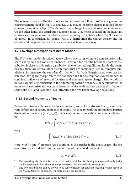
The self-consistency of K-V distribution can be shown as follows. K-V beams generatingelectromagnetic field in Eq. 3.3 and Eq. 3.4, results in space-charge-modified linearequation of motion of Eqs. 3.7 with linear space charge forces and invariant emittances.On the other hand, the distribution function in Eq. 3.8, which is based on the invariantemittances, can generate the electric potential in Eq. 3.12, from which Eq. 3.3 can beobtained. In conclusion, for beams with K-V distribution the charge density and theelectric and magnetic fields are associated in a self-consistent way.
3.2 Envelope Descriptions of Beam Motion
The K-V beam model described above allows one to investigate beam behavior withspace charge in a self-consistent manner. However, for realistic beams the particle dis-tribution is close to a Gaussian distribution due to thermal equilibrium inside the beam.Besides, there are sereral other distributions that are commonly used in computer sim-ulations, for instance, the waterbag distribution4. For both Gaussian and waterbag dis-tribution, the space charge forces are nonlinear and the distribution evolves under thecombined influence of external focusing and nonlinear space charge. The two distri-butions are not self-consistent in the alternating focusing channels in accelerators5. Inorder to characterize and compare beam dynamics with various particle distributions,Lapostolle [12] and Sacherer [13] introduced the rms beam envelope equations.
3.2.1 Second Moments of Beams
Before we introduce the rms envelope equations, we will first discuss briefly some rele-vant definitions of second moments of beams. For a beam with the normalized particledistribution function f (x , x ′, y, y ′), the second moment in x-direction can be obtainedby
⟨x2⟩=∫
x2 f (x , x ′, y, y ′)d xd yd x ′d y ′, (3.13)
with∫
f (x , x ′, y, y ′)d xd x ′d yd y ′ = 1. (3.14)
Here, x , x ′, y and y ′ are transverse coordinates of particles in the phase space. The rmsbeam size (in x) is defined as the square root of the second moment of x ,
σx =Æ
⟨x2⟩, (3.15)
4 The waterbag distribution is characterized with particles distributing random-uniformly insidethe hypersphere in four-dimensional phase space. For more details see Ref.[54].
5 The two distributions can be shown to be self-consistent for constant focusing system based onthe Vlasov-Maxwell approach. For more details see Ref.[54].
3.2. Envelope Descriptions of Beam Motion 33
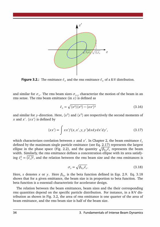
o
Figure 3.2.: The emittance εx and the rms emittance εx of a K-V distribution.
and similar for σy . The rms beam sizes σx ,y characterize the motion of the beam in anrms sense. The rms beam emittance (in x) is defined as
εx =Æ
⟨x2⟩⟨x2⟩ − ⟨x x ′⟩2 (3.16)
and similar for y-direction. Here, ⟨x2⟩ and ⟨x2⟩ are respectively the second moments ofx and x ′. ⟨x x ′⟩ is defined by
⟨x x ′⟩=∫
x x ′ f (x , x ′, y, y ′)d xd yd x ′d y ′, (3.17)
which characterizes corelation between x and x ′. In Chapter 2, the beam emittance εz
defined by the maximum single particle emittance (see Eq. 2.17) represents the largestellipse in the phase space (Fig. 2.2), and the quantity
Æ
β0,z εz represents the beamwidth. Similarly, the rms emittance defines a concentration ellipse with its area satisfy-ing ε2
z = (εz)2, and the relation between the rms beam size and the rms emittances is
σz =Æ
β0,z εz . (3.18)
Here, z denotes x or y. Here β0,z is the beta function defined in Eqs. 2.9. Eq. 3.18shows that for a given emittance, the beam size is in proportion to beta function. Thebeta function is a essentail characteristic for accelerator design.
The relation between the beam emittances, beam sizes and the their correspondingrms quantities depend on the specific particle distribution. For instance, in a K-V dis-tribution as shown in Fig. 3.2, the area of rms emittance is one quarter of the area ofbeam emittance, and the rms beam size is half of the beam size.
34 3. Fundamentals of Intense Beam Dynamics
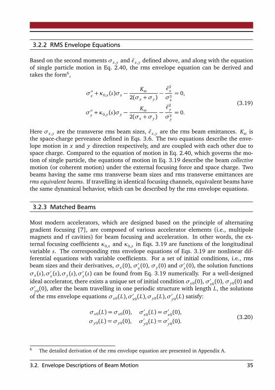
3.2.2 RMS Envelope Equations
Based on the second moments σx ,y and εx ,y defined above, and along with the equationof single particle motion in Eq. 2.40, the rms envelope equation can be derived andtakes the form6,
σ′′x +κ0,x (s)σx −Ksc
2(σx +σy)−ε2
x
σ3x
= 0,
σ′′y + κ0,y(s)σy −Ksc
2(σx +σy)−ε2
y
σ3y
= 0.
(3.19)
Here σx ,y are the transverse rms beam sizes, εx ,y are the rms beam emittances. Ksc isthe space-charge perveance defined in Eqs. 3.6. The two equations describe the enve-lope motion in x and y direction respectively, and are coupled with each other due tospace charge. Compared to the equation of motion in Eq. 2.40, which governs the mo-tion of single particle, the equations of motion in Eq. 3.19 describe the beam collectivemotion (or coherent motion) under the external focusing force and space charge. Twobeams having the same rms transverse beam sizes and rms transverse emittances arerms equivalent beams. If travelling in identical focusing channels, equivalent beams havethe same dynamical behavior, which can be described by the rms envelope equations.
3.2.3 Matched Beams
Most modern accelerators, which are designed based on the principle of alternatinggradient focusing [7], are composed of various accelerator elements (i.e., multipolemagnets and rf cavities) for beam focusing and acceleration. In other words, the ex-ternal focusing coefficients κ0,x and κ0,y in Eqs. 3.19 are functions of the longitudinalvariable s. The corresponding rms envelope equations of Eqs. 3.19 are nonlinear dif-ferential equations with variable coefficients. For a set of initial conditions, i.e., rmsbeam sizes and their derivatives, σx (0), σ′x (0), σy(0) and σ′y(0), the solution functionsσx (s),σ′x (s),σy(s),σ′y(s) can be found from Eq. 3.19 numerically. For a well-designedideal accelerator, there exists a unique set of initial condition σx0(0), σ′x0(0), σy0(0) andσ′y0(0), after the beam travelling in one periodic structure with length L, the solutionsof the rms envelope equations σx0(L),σ′x0(L),σy0(L),σ′y0(L) satisfy:
σx0(L) = σx0(0), σ′x0(L) = σ′x0(0),
σy0(L) = σy0(0), σ′y0(L) = σ′y0(0).
(3.20)
6 The detailed derivation of the rms envelope equation are presented in Appendix A.
3.2. Envelope Descriptions of Beam Motion 35

0 1 2 3 4 5
focusing periods
−2.0
−1.5
−1.0
−0.5
0.0
0.5
1.0
1.5
2.0
beam
envelopes
[cm]
matched
mismatched
Figure 3.3.: An example of numerical solutions of Eqs. 3.19. The rms envelopes of thematched beam and a mismatched beam in five alternating gradient focusingperiods.
Here we use the subscript ‘0’ after x and y to denote the matched case. The solu-tion satisfying Eq. 3.20 is called matched solution, and the beam in such case is calledmatched beam. For a matched beam, after transported one periodic structure, the sec-ond moments of the beam are equal to the initial values7. Since the envelope equationsdescribe the beam motion under the lattice structure and the space charge effect. Thebeam satisfying Eqs. 3.20 is matched to both the lattice and space charge.
The envelope equations in Eqs. 3.19 can be solved numerically. Using a numerical it-erative solution method (the shooting method for instance [60]), the matched sloutioncan be found. Fig. 3.3 illustrates an example of a mathced beam and a mismatchedbeam in five peroidic cells of the SIS-18 lattice. More details about the numerical algo-rithm will be discussed in the next chapter.
3.2.4 Space-Charge Modified Twiss Parameters
The Twiss parameters β0,z , α0,z , and γ0,z defined in Section 2.1.2 are basic character-istics of an accelerator, and are dependent on the configuration of the accelerator, forexample, the external focusing strengths of multipole magnets, and specific sequence ofaccelerator elements. In the presence of space charge in a high-intensity beam travellingin an accelerator, the external focusing strengths are depressed due to defocusing spacecharge. To characterize the effective focusing acted on the beam, the concept of space-
7 It is worth pointing out that while the second moments of the beam recover to the initial values,for each inidividual particle, the coordinates x and x ′ are different from the initial values.
36 3. Fundamentals of Intense Beam Dynamics

charge-modified Twiss parameters is introduced, based on the matched solutions of therms envelope equations. For example, similar to the Eq. 3.18, the space-charge-modifiedbeta function βz is defined as
βz =σz0
2
εz. (3.21)
Here, z denotes x or y. The other two Twiss parameters can be obtained by αz =−(βz)′/2 and γz = (1+α2
z )/βz . The space-charge-modified Twiss parameters, which aredependent on both accelerator configurations and the beam properties, characterize theinteraction between the beam envelope motion and the space charge within the beamin a self-consistent way. Equivalent beams travelling in identical accelerator channelshave the identical space-charge-modified Twiss parameters.
Analogy to the definition for the phase advance of the motion of a single particle inEq. 2.10, the space-charge-modified phase advance for a high-intensity beam can bedefined as
kz(s) =
∫ s
0
dsβz(s)
= εz
∫ s
0
dsσ2
z0
. (3.22)
Clearly, the space-charge depressed phase advance is decreasing with space charge in-creasing. It plays a key role in the analysis of beam instability, which will be discussedin the following.
3.2.5 Smooth Approximation
When the variation of the transverse beam size during one focusing period is muchsmaller than the average transverse beam size, the alternating focusing structure can beapproximated by a constant focusing structure, with the periodic focusing forces κ0,x (s)and κ0,y(s) replaced by their average constant values κ0,x and κ0,y . The equations ofenvelope become
σ′′x + κ0,x σx −Ksc
2(σx + σy)−ε2
x
σ3x
= 0,
σ′′y + κ0,y σy −Ksc
2(σx + σy)−ε2
y
σ3y
= 0.
(3.23)
This is usually called the smooth approximation in literatures [61]. For a constantfocusing structure, the transverse rms beam sizes of a matched beam are constant. It
3.2. Envelope Descriptions of Beam Motion 37

means that the matched solution of Eqs. 3.23 can be solved from the correspondingalgebraic equations
κ0,x σx0 −Ksc
2(σx0 + σy0)−ε2
x
σ3x0
= 0,
κ0,y σy0 −Ksc
2(σx0 + σy0)−ε2
y
σ3y0
= 0.
(3.24)
One of the most significant advantages of the smooth approximation is that the matchedsolution of Eqs. 3.23 σx0 and σy0, which can be seen as the approximated matchedsolution of Eqs. 3.19, can be found easily by solving Eqs. 3.24.
3.3 Beam Envelope Instabilities
The matched solutions of beam envelope equations are of essential important in accel-erator design and research, since they represent the maximum beam intensity that canbe transported in an accelerator channel. In practice, however, an ideal matched beamis difficult to achieve, since there are always exist magnet imperfections, misalignment,ion sources errors and so on. Beams in realistic cases perform envelope mismatch os-cillations around the matched solutions, as shown in Fig. 3.3. The amplitudes of themismatch oscillations are usually much smaller than the average rms beam size, whichallow a good beam travelling in accelerators. Sometimes for a beam with sufficientbeam in certain accelerator configurations, the beam mismatch oscillations lead to theinstability of the beam. In this subsection we perform to analyze the properties ofmismatch oscillation and introduce the well-known envelope instability [17].
3.3.1 Mismatch Oscillations
Let us start with slightly mismatched rms envelopes σx ,σy with small perturbations ξ,ζ
σx = σx0 + ξ,
σy = σy0 + ζ,(3.25)
where σx0 and σy0 are the matched solutions of Eq. 3.19. Substituting Eq. 3.25 intoEq. 3.19 and neglecting the higher order terms, we obtain the perturbation equations
ξ′′ +κ0,xξ+Ksc
2(σx0 +σy0)2(ξ+ ζ) +
3ε2x
σ4x0
ξ= 0,
ζ′′ + κ0,yζ+Ksc
2(σx0 +σy0)2(ξ+ ζ) +
3ε2y
σ4y0
ζ= 0,
(3.26)
38 3. Fundamentals of Intense Beam Dynamics

Figure 3.4.: Schematic drawing of the oscillations of the two eigenmodes.
0.0 0.2 0.4 0.6 0.8 1.0ηx
60
70
80
90
100
110
120
φ1,2[deg]
φ1
φ2
φ1,2
Figure 3.5.: Round beam case,k0,x = k0,y = k0 = 60: Phase shifts ϕ1,2 of the fundamen-tal mismatch oscillation versus tune depression in x .
which is a coupled differential equation system with its coefficients being functionsof the matched beam sizes (σx0 and σy0). Two envelope modes in Eqs. 3.26 can bedecoupled to characterize the mismatch oscillations. To show the properties of theenvelope modes, for simplity here we take an example of mismatch oscillation of around beam with σx0 = σy0, and εx = εy travelling in a symmetric constant focusingchannel. The phase shifts of the two envelope modes are8
ϕ1 =q
k20,z + 3k2
z , ϕ2 =q
2k20,z + 2k2
z . (3.27)
Here k0,z and kz is the phase advance without and with space charge, respectively. ϕ1
and ϕ2 represents the phase shifts of the two modes, i.e., the well-known quadrupolarmode and the breathing mode9. The mismatch oscillations characterized by the twoenvelope modes are schematiclly shown in Fig. 3.4. The blue solid line denotes thetransverse cross section of a matched round beam, and the red dashed lines are themismatch oscillations.
8 For details of the derivation see Appendix B.9 In many literatures, the two modes are also named as “fast mode” and “slow mode”.
3.3. Beam Envelope Instabilities 39
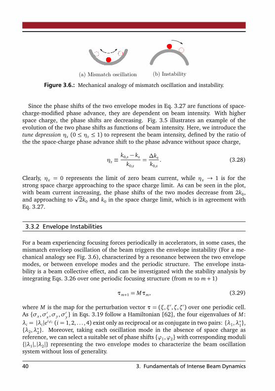
Figure 3.6.: Mechanical analogy of mismatch oscillation and instability.
Since the phase shifts of the two envelope modes in Eq. 3.27 are functions of space-charge-modified phase advance, they are dependent on beam intensity. With higherspace charge, the phase shifts are decreasing. Fig. 3.5 illustrates an example of theevolution of the two phase shifts as functions of beam intensity. Here, we introduce thetune depression ηz (0 ≤ ηz ≤ 1) to represent the beam intensity, defined by the ratio ofthe the space-charge phase advance shift to the phase advance without space charge,
ηz ≡k0,z − kz
k0,z=∆kz
k0,z. (3.28)
Clearly, ηx = 0 represents the limit of zero beam current, while ηx → 1 is for thestrong space charge approaching to the space charge limit. As can be seen in the plot,with beam current increasing, the phase shifts of the two modes decrease from 2k0,and approaching to
p2k0 and k0 in the space charge limit, which is in agreement with
Eq. 3.27.
3.3.2 Envelope Instabilities
For a beam experiencing focusing forces periodically in accelerators, in some cases, themismatch enveloep oscillation of the beam triggers the envelope instability (For a me-chanical analogy see Fig. 3.6), characterized by a resonance between the two envelopemodes, or between envelope modes and the periodic structure. The envelope insta-bility is a beam collective effect, and can be investigated with the stability analysis byintegrating Eqs. 3.26 over one periodic focusing structure (from m to m+ 1)
τm+1 = Mτm, (3.29)
where M is the map for the perturbation vector τ = (ξ,ξ′,ζ,ζ′) over one periodic cell.As σx ,σ′x ,σy ,σ′y in Eqs. 3.19 follow a Hamiltonian [62], the four eigenvalues of M :λi = |λi |eiϕi (i = 1, 2, . . . , 4) exist only as reciprocal or as conjugate in two pairs: λ1,λ∗1,λ2,λ∗2. Moreover, taking each oscillation mode in the absence of space charge asreference, we can select a suitable set of phase shifts ϕ1,ϕ2with corresponding moduli|λ1|, |λ2| representing the two envelope modes to characterize the beam oscillationsystem without loss of generality.
40 3. Fundamentals of Intense Beam Dynamics
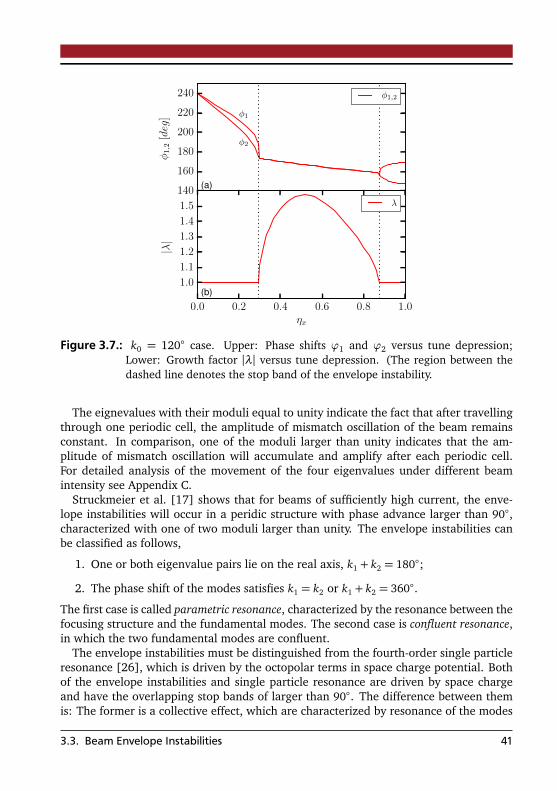
140
160
180
200
220
240
φ1,2[deg]
(a)
φ1
φ2
φ1,2
0.0 0.2 0.4 0.6 0.8 1.0ηx
1.0
1.1
1.2
1.3
1.4
1.5
|λ|
(b)
λ
Figure 3.7.: k0 = 120 case. Upper: Phase shifts ϕ1 and ϕ2 versus tune depression;Lower: Growth factor |λ| versus tune depression. (The region between thedashed line denotes the stop band of the envelope instability.
The eignevalues with their moduli equal to unity indicate the fact that after travellingthrough one periodic cell, the amplitude of mismatch oscillation of the beam remainsconstant. In comparison, one of the moduli larger than unity indicates that the am-plitude of mismatch oscillation will accumulate and amplify after each periodic cell.For detailed analysis of the movement of the four eigenvalues under different beamintensity see Appendix C.
Struckmeier et al. [17] shows that for beams of sufficiently high current, the enve-lope instabilities will occur in a peridic structure with phase advance larger than 90,characterized with one of two moduli larger than unity. The envelope instabilities canbe classified as follows,
1. One or both eigenvalue pairs lie on the real axis, k1 + k2 = 180;
2. The phase shift of the modes satisfies k1 = k2 or k1 + k2 = 360.
The first case is called parametric resonance, characterized by the resonance between thefocusing structure and the fundamental modes. The second case is confluent resonance,in which the two fundamental modes are confluent.
The envelope instabilities must be distinguished from the fourth-order single particleresonance [26], which is driven by the octopolar terms in space charge potential. Bothof the envelope instabilities and single particle resonance are driven by space chargeand have the overlapping stop bands of larger than 90. The difference between themis: The former is a collective effect, which are characterized by resonance of the modes
3.3. Beam Envelope Instabilities 41
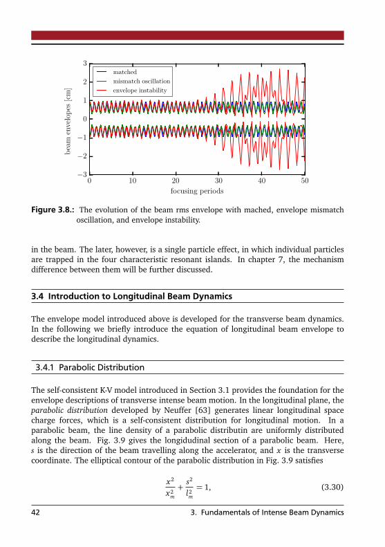
0 10 20 30 40 50
focusing periods
−3
−2
−1
0
1
2
3beam
envelopes
[cm]
matched
mismatch oscillation
envelope instability
Figure 3.8.: The evolution of the beam rms envelope with mached, envelope mismatchoscillation, and envelope instability.
in the beam. The later, however, is a single particle effect, in which individual particlesare trapped in the four characteristic resonant islands. In chapter 7, the mechanismdifference between them will be further discussed.
3.4 Introduction to Longitudinal Beam Dynamics
The envelope model introduced above is developed for the transverse beam dynamics.In the following we briefly introduce the equation of longitudinal beam envelope todescribe the longitudinal dynamics.
3.4.1 Parabolic Distribution
The self-consistent K-V model introduced in Section 3.1 provides the foundation for theenvelope descriptions of transverse intense beam motion. In the longitudinal plane, theparabolic distribution developed by Neuffer [63] generates linear longitudinal spacecharge forces, which is a self-consistent distribution for longitudinal motion. In aparabolic beam, the line density of a parabolic distributin are uniformly distributedalong the beam. Fig. 3.9 gives the longidudinal section of a parabolic beam. Here,s is the direction of the beam travelling along the accelerator, and x is the transversecoordinate. The elliptical contour of the parabolic distribution in Fig. 3.9 satisfies
x2
x2m
+s2
l2m
= 1, (3.30)
42 3. Fundamentals of Intense Beam Dynamics

Figure 3.9.: Schematic drawing of the parabolic distribution, on which particles distributerandom-uniformly on the ellipse with the semi-major axis lm and the semi-minor axis xm.
and similar for the case in the y − s plane,
y2
y2m
+s2
l2m
= 1. (3.31)
The line charge density at the position s = s0 can be calculated by the area of theellliptical cross section
λs0 = %0πx0 y0 = %0 xm ym(1−s20
l2m
), (3.32)
in which %0 = is the uniform volume charge density, with Q is the total charge of thebeam. The line density at the beam center s = 0 is
λ0 =3Q4lm
(3.33)
Neuffer [63] showed that the parabolic distribution generates the longitudinal spacecharge forces insdie the beam, based which one can derive the longitudinal envelopeequation.
3.4.2 Longitudinal Envelope Equations
The linearized equations of synchrotron motion for a single particle of Eq. 2.28 takesthe form
d2ϕ
d t2=
hqηV cosϕs
2πEϕ, (3.34)
3.4. Introduction to Longitudinal Beam Dynamics 43

where ϕ and ϕs are the phase of the single particle and the synchronous particle. q andE = γm0c2 are the charge and the energy of the particle. h is the harmonic number,and η the slip factor. V is the rf voltage. With the relation dϕ/d t = β cdϕ/ds anddϕ = Rdz, (Here z is the longitudinal coordinate and R is the average radius of the syn-chrotron), for a beam with parabolic distribution, the longitudinal envelope equationscan be derived10 from Eq. 3.34
z′′m +κz0zm −KL
z2m
−ε2
L
z3m
= 0, (3.35)
in which, zm is the half length of the parabolic beam, and κz0 represents the linearizedexternal rf focusing strength given by
κz0 = qV cosϕshη/(2πR2γβ2m0c2). (3.36)
The linearized external focusing gradient modified by longitudinal space charge is κz =κz0 − KL/z
3m, with the longitudinal perveance KL = 3gN Z2rp/(2β2γ5A); the geometry
factor g = 0.5 + 2 ln(Rp/Rb) (Rp and Rb are the radii of the beam pipe and the beam,respectively); N the number of particles in the bunch; rp the classical proton radius andη the slip factor. εL is the longitudinal emittance, defined as
εL = |η|zmδ0, (3.37)
in which δ0 is the momentum spread at the center of the bunch. Physically, εL denotesthe area in longitudinal phase space, which is constant without acceleration.
10 For more details of derivation, see Ref. [54]
44 3. Fundamentals of Intense Beam Dynamics

4 Numerical Calculation and PICSimulation
In previous chapters, we have introduced the fundamentals of intense beam dynamics,including the dynamics of single particle and beam envelope motion. In the presenceof both external focusing and smoothed effect of the self field, an intense beam as awhole performs coherent behaviors described by the motion of its rms envelope, and itis unrealistic and unnecessary to calculate the Lorenz force acted on each particle in thebeam. Before we further investigate the motion of intense beams, in this chapter weshall pay specific attention to two main approaches adopted in the following chapters:the numerical calculation and particle-in-cell simulation. Firstly, section 4.1 introducesthe method of numerical calculation. The scheme of simulation with space charge andthe relevant simulation code is briefly introduced in section 4.2. In section 4.3, com-parison of results of a few examples will be presented to show the benchmarking of thetwo methods.
4.1 Numerical Calculation
The rms envelope approach and the concept of equivalent beams form the foundationof the theory of beam dynamics with space charge. The solutions of matched beammotion can be obtained from the envelope equations of Eq. 3.19, and beam stabilitycan be analyzed by calculating the envelope modes from the mismatched oscillationsof Eq. 3.26. In the general case, coefficients of the envelope equations representingexternal focusing forces are piecewise functions of position s according to the principleof alternating gradient focusing. Mathematically, to obtain the analytical solution ofthe differential equations with variable coefficients is formidable, and the only possiblesolution for most cases is the numerical one.
In the work of this thesis, the matched solutions and envelope modes are numer-ically calculated via a envelope solver code “pyKV”1, written by Prof. Oliver Boine-Frankenheim, and further developed by the author. The code is written in Python [64]and consists of two script files, one (named as “pyLine”) is used to input the latticeparameters from output files of MAD-X [53]. Another file “pyEnvelope” is for solvingthe envelope equations as the initial parameters from the file “pyLine”. In the numeri-cal calculation, the iterative scheme and shooting method in the Python-based package
1 For instance, the envelope plots of Fig. 3.3 and Fig. 3.8, and the envelope modes in Fig. 3.5 andFig. 3.7 are all calculated from the numerical code.
45

Envelope solver
input initial parameters
initial conditions/guess value
solve envelope equations
matched solution
solve perturbation equations
(pyLine)
(pyEnvelope)
(pyPerturbation)
Figure 4.1.: Structure of the envelope solver code.
Numpy [65] and Scipy [66] are employed to find the matched solutions. The pertur-bative calculation can be achieved in the third script file “pyPerturbation”, in which,Newton’s method in matrix form is used to solve the envelope oscillation equationswith the matched solutions from “pyEnvelope” as the coefficients. The structure of theenvelope solver is shown in Fig 4.1.
4.2 PIC Simulaton
Another widely-used approach to study the beam dynamics is the simulation programsof particle-tracking. Various simulation programs are developed in many famous ac-celerator laboratories. In these programs, thousands of macro particles representingnumerous charged particles in real beams, are tracked based on accurate calculation ofthe equations of motion of each macro particle in both of electromagnetic fields of eachaccelerator components and the self field of the beam. The detailed information of theirmotion (coordinates, speed, energy) are recorded and output. With the advantage ofprecise controlling and flexible adjustment to beam parameters and nearly zero cost,simulation programs are powerful tools and widely used for the design, commissionand operation of accelerators.
4.2.1 Computational Model of Space Charge
For the simulation of intense beams, accurate calculation of space charge is of essentialimportance. The well-accepted computational model for treatment of space charge isthe scheme of particle-in-cell (PIC for short) [67, 68]. As shown in Fig. 4.2, for eachtime cycle, the distribution of particles in a beam is interpolated onto a grid, with thecharge assigned to grid nodes (Weighting). Then, the potential and the correspondinginterpolated electromagnetic fields is obtained from the solution of the Poisson equation(Integration). The electromagnetic forces, combined with external forces, are acted onparticles and the particle distribution is updated from the results of the combined forces.
In principle, the calculation of space charge is a three dimensional (3-D) problem,where a 3-D grid is required for weighting the 3-D particle distribution. This is the casefor linacs, where the transverse and longitudinal sizes of the bunch are comparable.
46 4. Numerical Calculation and PIC Simulation

Integration of equations
of motion, moving particles
Weighting
Integration of field
equations on grid
Weighting
Figure 4.2.: A typical cycle of PIC in a particle simulation program. The particle arenumbered as i, the grid indices are j. (Figure from Ref. [68])
However, for circular accelerators, where the longitudinal bunch size is much largerthan transverse size, an alternative method of “2.5-D space charge model” is widelyused. In the 2.5-D scheme, the 3-D particle distribution is interpolated onto a set of 2-Dgrids transversely and a set of slices longitudinally. Transverse space charge is calculatedfrom PIC scheme solving the 2-D Poisson equations, and longitudinal space charge areevaluated based on the fluctuations of the linear charge density of the beam. For thecase of coasting beams, where longitudinal fluctuations is absent, transverse beam pro-file is independent on the longitudinal position. This allows us to reduce the calculationof transverse space charge fields to a 2D problem. For the case of long bunched beams,however, the longitudinal fluctuation in line density (longitudinal space charge), andthe problem of long bunched beams is 2.5-D. In the 2.5-D PIC simulation, the numberof grid points for 2-D transverse space charge is chosen to be sufficiently large to re-duce the grid dependent noise [69], and the number of slices for 1-D longitudinal spacecharge are checked by obtaining a smooth longitudinal space charge force.
4.2.2 PyORBIT
In the work of this thesis, the simulation code PyORBIT [70] is used to perform particletracking with space charge. pyORBIT is a modern implementation of the original ORBIT(Objective Ring Beam Injection and Tracking) [71] that was developed at Oak RidgeNational Laboratory to improve the Spallation Neutron Source accelerator ring designand to study proton beam dynamics in the presence of collective effects.
In pyORBIT, macro particles are contained in bunches and can interact with eachother via self fields (space charge) or through the electromagnetic fields induced in theaccelerator elements (impedances). At present, PyORBIT has two space charge modelsfor linacs and one for rings: For linacs there are two alternative methods in pyORBIT:
4.2. PIC Simulaton 47

Figure 4.3.: Comparison of rms beam size for three periodic cell between simulations andenvelope equation.
3-D uniformly charged ellipsoid field and a 3-D FFT Poisson solver. For circular accel-erators, the 2.5-D PIC scheme based on the convolution method [67] is employed inpyORBIT.
4.3 Benchmarking and Comparison
In order to show the correctness and effectiveness of the two approaches of the numer-ical envelope calculation and PIC simulations, in this section we give three examples,each of which has the results from the two methods.
In the first example, we calculate the transverse rms size of a beam transported inperiodic cells of the SIS-100 synchrotron. Both effects of space charge and dispersionare considered2. As shown in Fig. 4.3, the solid line represents the rms beam sizecalculated from envelope approach, and the dotted line represents the rms beam sizeat the entrance of each element obtained from PIC simulation. It is shown that the tworesluts are in good agreement.
The second example is the benchmarking of space charge calculation. Fig.4.4 showsthe space charge forces acted on each macro particle inside a K-V beam, calculated bythe PIC solver in the code pyORBIT, compared with the theoretical results by using theformula of the space charge perveance in Eq. 3.6. It can be seen that for K-V beams, thedistribution of space charge forces obtained from PIC solver is linear and agrees wellwith the theory.
In the third example, we show space-charge tune spread in a beam with Gaussiandistribution, truncated at 3σ (here σ is the standard deviation.). The bare tune Q0,x =
2 For details of intense motion with dispersion see chapter 6
48 4. Numerical Calculation and PIC Simulation

Figure 4.4.: Comparison of the transverse space charge forces in a K-V beam calculatedfrom pyORBIT and theoretical formula.
Figure 4.5.: Comparison of the space-charge tune spread in a Gaussian beam calculatedfrom pyORBIT and theoretical formula.
4.3. Benchmarking and Comparison 49

4.64, Q0,y = 2.78, as shown in Fig. 4.5. The diamond in write line represents the tunespread from a theoretical formula [72], the color area, which fills the write line, denotesthe distribution of space-charge depressed tune for the Gaussian beam, obtained frompyORBIT. It can be seen that the color area mainly fills at the lower half part of thediamond. This is because the edge particles, which has small tune spread, has been cutoff in the truncated Gaussian distribution.
50 4. Numerical Calculation and PIC Simulation

5 Complete Set of Second-MomentInstabilities
The envelope equations introduced in Chapter 3 are based on the second momentsof beams. The corresponding envelope modes, which characterize the beam envelopeoscillations and envelope instabilities, are also well-known as the “second order evenmodes”. Besides the even modes, there exists second order odd modes1. Differentfrom the even modes, which are led by the mismatched oscillations of rms beam sizes,the odd modes are caused by the coupling effects between the two transverse direc-tions (x and y), either from self rotation of the beam, or external skew strength, e.g.,skew quadruple or solenoid. Analogy to the fact that the second order even modescan trigger the envelope instability, the second order odd modes can trigger the “tiltinginstability”, characterized with the resonant emittance exchange by space charge cou-pling [73, 74, 75]. Furthermore, in periodic focusing channel with sufficiently differentphase advances, the “sum envelolpe instability” can be excited by either the secondorder even modes, or the odd modes [22, 76].
In this chapter, we will present the complete set of second-moment instabilities drivenby the second order even and odd modes and their sum effects. This is achieved by em-ploying a unified equation set of second-moment oscillations derived from the “Cherninequations” 2.
This chapter is organized as follows. In section 5.1, we first extract the second-moment oscillation equations without external skew strength from Chernin equations.This is followed by calculating the frequencies of second order odd modes and showingthe “tilting instability”in a constant focusing structure in section 5.2; furthermore acomparison with the results derived from Vlasov-Maxwell equation in Ref. [1], as wellas a Fourier analysis of noise spectra from a 2-D PIC simulation. Finally, in section 5.3we explore the theoretical mechanism of sum envelope instabilities, including both thecoupled even mode sum instability and the odd mode sum instability. Full stop bandsare calculated and compared with PIC simulation results including particle evolution inreal space.
For clarity, in the following we assume x and y are the transverse degrees in horizon-tal and vertical direction, respectively; s the longitudinal coordinate; and k0,x ,y , kx ,y arethe phase advances per focusing cell without and with space charge, respectively. ϕ1
and ϕ2 (ϕ1 > ϕ2) denote the phase shifts of the second order even modes (i.e., the twoenvelope modes), while ψ1, ψ2 (ψ1 > ψ2) are the phase shifts of the two second orderodd modes, respectively.1 The second order modes are also known as “skew modes”.2 Written as “Chernin equations” in the following, for more details see Ref. [5].
51

5.1 Second-Moment Oscillations
We first consider a lattice including an external skew focusing force. Following Chernin,the evolution of second moments of the beam can be written in matrix form [5]
Σ′ = MΣ+ (MΣ)T , (5.1)
with
M =
0 1 0 0−κx (s) 0 −qx y(s) 0
0 0 0 1−qx y(s) 0 −κy(s) 0
. (5.2)
Here, “ ′ ” denotes the derivative with respect to s, the superscript “T” means thetransposed matrix, Σ represents the 4 × 4 matrix of the second moments, with ele-ments Σi j defined by Σi j ≡ ⟨νiν j⟩ − ⟨νi⟩⟨ν j⟩, where the averages are taken over thephase space variables and the subscripts i, j run from 1 to 4 representing x , x ′, y, y ′.κx = κx0 −∆κx , κy = κy0 −∆κy and qx y = qx y,0 −∆qx y , with κx0 = (1/B%)(∂ By/∂ x),κy0 = −(1/B%)(∂ Bx/∂ y) the external focusing gradients and qx y0 = (1/B%)(∂ Bx/∂ x)the external linear coupling, (B% is the magnetic rigidity) and ∆κx , ∆κy and ∆qx y thespace-charge induced shifts, defined by
∆κx =Ksc
2
Sy
S0(Sx + Sy), ∆κy =
Ksc
2Sx
S0(Sx + Sy),
∆qx y =Ksc
2Σ13
S0(Sx + Sy),
(5.3)
using
S0 =q
Σ11Σ33 −Σ213,
Sx = Σ11 + S0, Sy = Σ33 + S0.(5.4)
Here Ksc is the space charge perveance parameter defined in Eqs. 3.6. Clearly, Σ13, Σ14,Σ23 and Σ24 denote the coupling moments between x and y. Eq. 5.1 can be written ina concise form [77]
Σ′ = G(Σ(s), s). (5.5)
For a lattice with constant focusing and coupling, Eq. 5.5 can be readily solved with agiven initial generalized emittance [78]. For a lattice with alternating-gradient focus-ing, matched solutions Σ0(s) can be obtained numerically from Eq. 5.5 with periodicconditions Σ0(s) = Σ0(s+ L), where L is the periodicity.
52 5. Complete Set of Second-Moment Instabilities

Now let us assume a slightly mismatched case, where the second moments can bewritten as Σ(s) = Σ0(s) + Σp(s)3. After Taylor expanding and keeping only first orderterms we have from Eq. 5.5
Σ′ = (Σ0 +Σp)′ = G(Σ0) + J(Σp), (5.6)
which can be divided into two parts
Σ0′ = G(Σ0), Σ′p = J(Σ0)Σp . (5.7)
Here J represents the Jacobian matrix of G with elements Jk,l = ∂ Gk(Σl)/∂Σl , with k, lrun from 1 to 10 along the possible combinations of the second order moments Σi j .
After several steps of derivations4, the complete set of second-moment oscillation canbe written as two parts, with the first part
Σp11′ = 2Σp
12,
Σp12′ =
∂ G2
∂Σ11
0Σ
p11 +
∂ G2
∂Σ12
0Σ
p12 +
∂ G2
∂Σ33
0Σ
p33,
Σp33′ = 2Σp
34,
Σp34′ =
∂ G8
∂Σ11
0Σ
p11 +
∂ G8
∂Σ33
0Σ
p33 +
∂ G8
∂Σ34
0Σ
p34,
(5.8)
which are recognized as envelope oscillations, and the second part
Σp13′ = Σp
14 +Σp23,
Σp14′ =
∂ G4
∂Σ13
0Σ
p13 +Σ
p24,
Σp23′ =
∂ G5
∂Σ13
0Σ
p13 +Σ
p24,
Σp24′ =
∂ G6
∂Σ13
0Σ
p13 +
∂ G6
∂Σ14
0Σ
p14 +
∂ G6
∂Σ23
0Σ
p23.
(5.9)
which is for the equations of second order odd modes. Here the cofficients in Eqs. 5.8and Eqs. 5.9 are partial derivatives of the Jacobian matrix G with respect to the secondmoments5. With matched solutions of the second moments of beams from Eq. 5.1, theabvoe two equations are used to calcualte the second order modes.
3 The subscript “0” and “p” denotes respectively the matched solution and a small perturbationof the matched solution.
4 For mathmatical details see Appendix D.5 Appendix G lists each value of the derivatives for the case without external skew focusing forces.
5.1. Second-Moment Oscillations 53

5.2 Tilting Instability in Constant Focusing
In this section, we will investigate the instability induced by the odd modes for in-tense beams transported in a constant focusing channel6, by using the set of oscillationequations in Eq. 5.8 and Eq. 5.9. For constant focusing Eqs. 5.9 take the form
d2
ds2Σ
p13 = a1Σ
p13 + a2Σ
p24,
d2
ds2Σ
p24 = a3Σ
p13 + a4Σ
p24,
(5.10)
with the coefficients
a1 = ∂ qx y
∂Σ13(Σ11 +Σ33)− (kx + ky)
0,
a2 = 2,
a3 =
−∂ qx y
∂Σ13(kxΣ11 + kyΣ33) + 2kx ky
0,
a4 = −(kx + ky)0.
(5.11)
The two odd modes with the corresponding phase shiftsψ1,2 can be readily decoupledand obtained from Eq. 5.10. For a round beam under a symmetric constant focusingwith k0,x = k0,y = k0, the results of odd modesψ1,2 calculated numerically from Eq. 5.10,along with the even ones ϕ1,2 from Eq. 5.8, are shown in Fig. 5.1 for different beamcurrents in units of the space charge tune depression ηx ≡ (k0,x−kx )/k0,x . It can be seenthat due to the axial symmetry the fast branch of the odd modes ψ1 is always identicalwith the slow branch of the even mode, while the slow odd mode ψ2 is zero (not shownin the plot). This is in agreement with the results obtained from Vlasov equation for theround beam case in Ref.[1].
The tilting instability is induced by a sufficiently large asymmetry of the transversefocusing, where the transverse beam shape becomes elliptical, the slow branch of theodd modes become nonzero. An example with k0,x = 60 and k0,y = 66.7 and εx/εy = 2is shown in Fig. 5.2. It is seen that the slow odd modeψ2 is close to ky−kx for increasingbeam current up to the point, where both become zero. In this region the slow odd modeis called a “difference mode”. To the right side of this point in Fig. 5.2, (ψ2)2 becomesnegative, hence unstable, and the imaginary part is shown. This “tilting instability” isdiscussed in detail further below. For the fast odd mode ψ1 ≥ kx + ky , hence this modecan be called “sum mode”.
PIC simulations using PyORBIT [70] are performed to compare with results from thisanalytical framework. To this end 50 000 macro particles are tracked over 1000 periodicFODO cells, and a Fourier analysis is employed on the coupling moment ⟨x y⟩ at various
6 It can be shown that for constant focusing, the even modes are always stable, see Ref.[1].
54 5. Complete Set of Second-Moment Instabilities
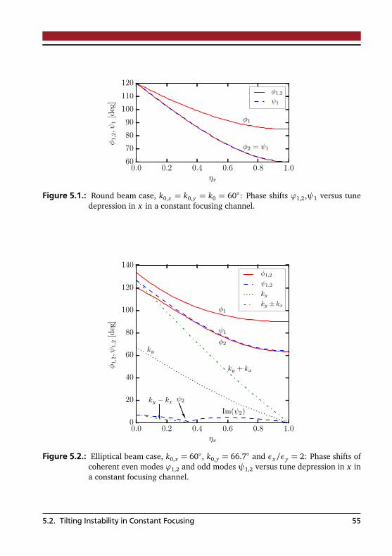
0.0 0.2 0.4 0.6 0.8 1.0ηx
60
70
80
90
100
110
120
φ1,2,ψ
1[deg]
φ1
φ2 = ψ1
φ1,2
ψ1
Figure 5.1.: Round beam case, k0,x = k0,y = k0 = 60: Phase shifts ϕ1,2,ψ1 versus tunedepression in x in a constant focusing channel.
0.0 0.2 0.4 0.6 0.8 1.0ηx
0
20
40
60
80
100
120
140
φ1,2,ψ
1,2[deg]
ky + kx
ψ1
φ1
φ2
ψ2
Im(ψ2)
ky
ky − kx
φ1,2
ψ1,2
ky
ky ± kx
Figure 5.2.: Elliptical beam case, k0,x = 60, k0,y = 66.7 and εx/εy = 2: Phase shifts ofcoherent even modes ϕ1,2 and odd modes ψ1,2 versus tune depression in x ina constant focusing channel.
5.2. Tilting Instability in Constant Focusing 55

ηx = 0.95KVWB
ηx = 0.9
ηx = 0.8
0 20 40 60 80 100 120 140 160 180
beam spectrum of 〈xy〉 [deg]
Pow
er[arb.units]
ηx = 0.7
Figure 5.3.: Elliptical beam case, k0,x = 60, k0,y = 66.7: Beam spectrum of ⟨x y⟩ fromPIC simulation of KV distribution (red solid) and waterbag (WB) distribution(blue solid), compared with the analytical results (dotted black lines) of phaseshifts of second order odd sum and difference modesψ1,2, for different valuesof ηx in a constant focusing channel.
beam intensities in terms of ηx . As shown in Fig. 5.3, the beam spectra of ⟨x y⟩ for a K-Vand a waterbag distribution agree well with the results of the second order odd modephase advances ψ1,2 in Fig. 5.2 obtained from the theoretical approach of Eq. 5.10.
Note the minor bump to the l.h.s. of the sum mode, which has a downwards shiftfrom ψ1 increasing roughly linearly with space charge. This might be associated withsingle particle tunes and numerical noise of the PIC code.
An interesting property of the second order odd modes shown in Ref. [1] is found forεx 6= εy and sufficiently large anisotropy. With an external focusing stronger in y thanin x (or vice versa), but reverted due to space charge, the beam is subject to the tiltinginstability with periodical exchange of emittances as indicated above in Fig. 5.2. In thiscase the solution of Eq. 5.9 shows that the squared phase shift of the difference modebecomes negative, (ψ2)2 < 0, indicating instability. As an example, Fig. 5.4 illustratesthe imaginary part of ψ2 for constant ky/k0,y = 0.8 and εx/εy = 2, as a function ofthe betatron tune ratio, hence the stop band of the tilting instability. We find that the
56 5. Complete Set of Second-Moment Instabilities

0.98 1.00 1.02 1.04 1.06 1.08 1.10
kx/ky
0.000
0.005
0.010
0.015
0.020
0.025
0.030
Imψ2/k
0,y
kxky
= 1k0,xk0,y
= 1
Figure 5.4.: Growth rate of difference odd mode (normalized) for constant ky/k0,y = 0.8and εx/εy = 2 as a function of the betatron tune ratio, indicating the tiltinginstability in a constant focusing channel.
values of growth rates as well as the width of the stop band are in excellent agreementwith the curve of the second order odd mode in Fig. 4 in Ref. [24], which is based onthe linearized Vlasov-Poisson approach - thus confirming the equivalence of these twomodels. Note that following Ref. [24] the tilting instability is accompanied by a - usually- dominant fourth order resonance in an adjacent stop band, which is the well-knownMontague instability (see also Ref. [75]).
5.3 Sum Envelope Instabilities in Periodic Focusing
In chapter 4 we introduced the well-known envelope instability in periodic focusinginduced by the unstable second order even modes. In this section, we will show thatbesides the envelope instability, the “sum envelope beam instability” exists in a periodic,unsymmetrical focusing channel, which is a coupling effect between x and y plane.Analogous to the mechanism of the well-known envelope instability, the sum envelopebeam instability is a resonant phenomenon of the second order modes, and can beclassified into two essentially distinct modes [22]
• Coupled even mode sum instability. Based on space charge coupling between evenenvelope modes and their parametric resonance with the lattice, the stop band ofcoupled even modes is theoretically illustrated in Figs. 1, 2 of Ref. [22].
• Skew (odd) mode sum instability. This instability is based on parametric resonanceof the odd sum mode as shown by the PIC simulation in Fig. 3 of Ref. [22].
In the following, we explore the theoretical mechanisms of both modes by using the for-malism of Eqs. 5.9. Similar to the treatment of the usual envelope instabilities [4, 17],
5.3. Sum Envelope Instabilities in Periodic Focusing 57

80
100
120
140
160
180
φ1,2,ψ
1,2[deg]
180 line (a)
360 − ψ1
ψ2
360 − φ1
φ2
360 − φ1, φ2
360 − ψ1, ψ2
0.0 0.1 0.2 0.3 0.4 0.5ηx
1.00
1.02
1.04
1.06
|λ|
(b)
skew modesum instability
coupled modesum instability
|λ||λ|
1.0
1.4
1.8
2.2
2.6
ǫ x/ǫ
x0
ǫx/ǫx0
Figure 5.5.: Perturbation theory results for both types of sum envelope instabilities in aperiodic focusing system. Upper plot (a): Phase shifts of ϕ1,2, ψ1,2 versestune depression in x; Lower plot (b): Corresponding growth factors per lat-tice period (continuous lines), and comparison with final emittance growthfactors (dashed lines, normalized to initial values) for PIC simulation of samecases.
the four eigenvalues can be calculated by integrating Eqs. 5.8 and Eqs. 5.9: ζm+1 = Mζm,where M is the map for the perturbation vector ζ= (Σp
11,Σp12,Σp
33,Σp34,Σp
13,Σp14,Σp
23,Σp24)
over one periodic cell. The eight eigenvalues of M , λi = |λi |eiϕi (i = 1,2, ...8), exist onlyas reciprocal or as conjugate. One of the moduli larger than unity can be used as growthfactor per lattice period of the sum envelope instabilities.
The example in Fig. 5.5 shows the second order even and odd modes as a function ofbeam intensity in an unsymmetrical FODO lattice with k0,x = 60 and k0,y = 145. Forconvenience of plotting, in Fig. 5.5(a) the curves of 360−ψ1 and 360−ϕ1 are plottedinstead of ψ1 and ϕ1. In the region kx = 44.2 to 39.6 (corresponding to ηx = 0.737 to0.66) one branch of the odd mode is locked to 180, with the corresponding eigenvaluelarger than unity, indicating the skew mode sum instability. It is characterized by theparametric resonance between the focusing structure and the odd sum mode branchψ1. Further increasing the beam current, ϕ2 and 360 − ϕ1 (the curves in red color)
58 5. Complete Set of Second-Moment Instabilities

Figure 5.6.: Real space distributions for three consecutive cells at early stage of coupledeven mode sum instability with initial ηx = 0.6.
become confluent, i.e., ϕ1 +ϕ2 = 360, which means the two even modes are coupledand the coupled mode sum instability is excited. Note that the width of the stop band ofthe skew mode sum instability is wider than the one of the coupled mode sum instability,and both stop bands are only separated by a thin gap.
The theory of second-moment oscilltion results abover provide no information onrms emittance growth. This requires PIC simulation with results shown by the dashed(green) lines in Fig. 5.5(b). The simulation results show εx/εx0 after 500 focusing peri-ods, at which time the emittance growth caused by the instability is already saturated.The initial particle distribution is chosen as rms-matched transverse waterbag. Two“sawtooth” like emittance growth phenomena are observed, with a width that agreeswell with the stop bands obtained from perturbation theory stop bands. The shape ofa “sawtooth” is caused by the self-detuning process, which is a remarkable feature ofthe second order coherent instabilities [20, 4]. Note that the saturated PIC emittancegrowth factor for the coupled mode sum instability is larger than that of the skew modesum instability, whereas the mode amplitude growth factor (per period) of the latterexceeds that of the former. Figs. 5.6 and 5.7 show the PIC simulation results in realspace projections at three consecutive periods at early stages of the two modes of insta-bility. In the case of the coupled even mode sum instability the beam shows a coupledmodulation of envelopes in x and y. In contrast, the beam performs skew “swinging”in real space as a characteristic of the skew mode sum instability.
Fig. 5.8 shows the change of phase shifts of the second order even and odd modes(in solid and dashed lines, respectively), with fixed k0,y = 145 and varying k0,x =40, 50, 60 and 70. The curves of 360 −ψ1 and 360 − ϕ1 are plotted instead ofψ1 and ϕ1. Two main properties can be observed and discussed as follows: Firstly,with k0,x increasing from 40 to 70, the sum instability starts to appear (in the case of
5.3. Sum Envelope Instabilities in Periodic Focusing 59
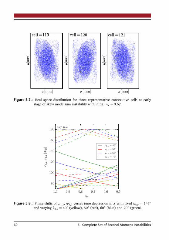
Figure 5.7.: Real space distribution for three representative consecutive cells at earlystage of skew mode sum instability with initial ηx = 0.67.
0.50.60.70.80.91.0ηx
80
100
120
140
160
180
φ1,2,ψ
1,2[deg]
180 line
k0,x = 40
k0,x = 50
k0,x = 60
k0,x = 70
Figure 5.8.: Phase shifts of ϕ1,2, ψ1,2 verses tune depression in x with fixed k0,y = 145
and varying k0,x = 40 (yellow), 50 (red), 60 (blue) and 70 (green).
60 5. Complete Set of Second-Moment Instabilities

Figure 5.9.: Tune diagram as scan of growth factor λ obtained from perturbation matrix.
Figure 5.10.: Enlarged scans of the two opposite corner zones in Fig. 5.9.
5.3. Sum Envelope Instabilities in Periodic Focusing 61
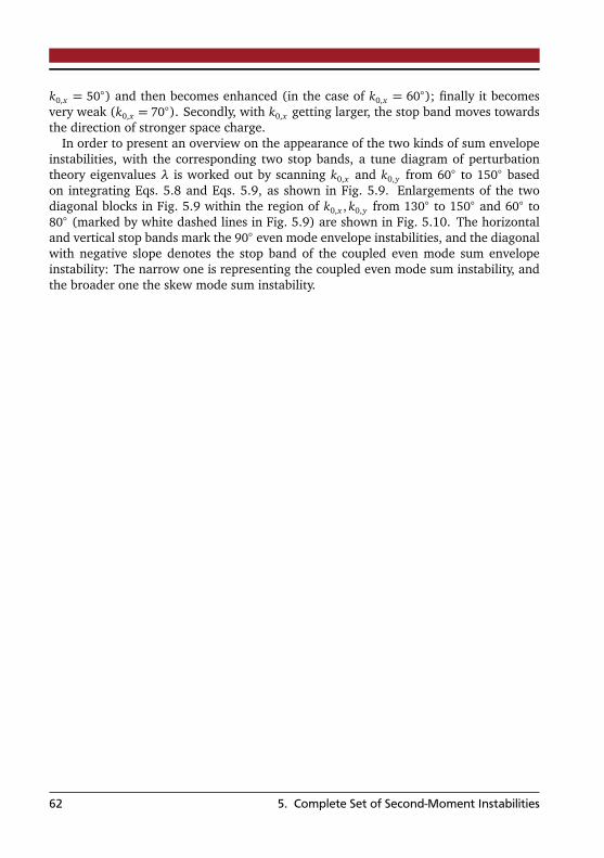
k0,x = 50) and then becomes enhanced (in the case of k0,x = 60); finally it becomesvery weak (k0,x = 70). Secondly, with k0,x getting larger, the stop band moves towardsthe direction of stronger space charge.
In order to present an overview on the appearance of the two kinds of sum envelopeinstabilities, with the corresponding two stop bands, a tune diagram of perturbationtheory eigenvalues λ is worked out by scanning k0,x and k0,y from 60 to 150 basedon integrating Eqs. 5.8 and Eqs. 5.9, as shown in Fig. 5.9. Enlargements of the twodiagonal blocks in Fig. 5.9 within the region of k0,x , k0,y from 130 to 150 and 60 to80 (marked by white dashed lines in Fig. 5.9) are shown in Fig. 5.10. The horizontaland vertical stop bands mark the 90 even mode envelope instabilities, and the diagonalwith negative slope denotes the stop band of the coupled even mode sum envelopeinstability: The narrow one is representing the coupled even mode sum instability, andthe broader one the skew mode sum instability.
62 5. Complete Set of Second-Moment Instabilities

6 Space-Charge Dominated BeamDynamics in Synchrotrons
As introduced in Chapter 1, the effect of dispersion is one of the most important char-acteristic for the motion of charged particles in a beam travelling in a synchrotron. Theaim of this chapter is dedicated to a detailed study of space-chagre dominated beamdynamics in synchrotrons, where the dispersion and space charge have a combined ef-fect on the beam. The envelope theory introduced in chapter 3 is generalized to thecase in which the role of dispersion is fully taken into for matched beam motion andmismatch oscillations. In the presence of space charge and dispersion, the mismatchoscillation could lead to the dispersion-induced instability [4], characterized by thecoherent dispersion mode, which will be discussed in detail.
The chapter is organized as follows. We introduced the generalized envelope equa-tions including dispersion in section 6.1, as well as some relevant concepts. The beamdynamics in matched and mismatched cases in the presence of both space charge anddispersion are discussed respectively in section 6.2 and 6.3. In section 6.4, the beam in-stabilities with space charge and dispersion, including the dispersion-induced instabilityand the dispersion-modified envelope instability are shown by both numerical approachand PIC simulations.
6.1 The Generalized Envelope Equations
6.1.1 Space-Charge Modified Dispersion
Consider a coasting beam transported in a periodic focusing channel with dipoles1. Forsimplicity, here we ignore any imperfection of the periodic channel and any nonlineareffect due to external focusing, as well as all the chromatic terms. The Hamiltonian ofsuch a system can be expressed as
H =12(p2
x + p2y) +
κx0(s)2
x2 +κy0(s)
2y2 +
m2c4
E20
δ2 −x%(s)
δ+ Vsc(x , y, s), (6.1)
where s is the longitudinal coordinate; κx0(s),κy0(s) denote the focusing gradients; %(s)the radius of curvature; δ = (p− p0)/p0 the fractional momentum deviation from thedesign momentum p0 with E0 being the corresponding energy and Vsc the space charge
1 This focusing channel can be seen as a periodic cell in a synchrotron.
63

potential. Following the framework in Ref. [29, 2] (written as “V-R and L-O theory”in the following), with a series of derivation of coordiante transformation and secondmoment distribution, the space-charge-modified dispersion function can be obtained2
d2Dx
ds2+
κx0(s)−Ksc
2X (X + Y )
Dx =1%(s)
, (6.2)
with the corresponding rms envelope equations in the presence of both dispersion andspace charge:
d2σx
ds2+
κx0(s)−Ksc
2X (X + Y )
σx −ε2
d x
σ3x
= 0, (6.3a)
d2σy
ds2+
κy0(s)−Ksc
2Y (X + Y )
σy −ε2
d y
σ3y
= 0. (6.3b)
Here, the second moments X and Y are the total transverse rms beam size includingdispersion; σx and σy are the betatron beam size with the relation
X =q
σ2x +σ
2δD2
x , Y = σy , (6.4)
where σδ is the rms momentum spread. It can be seen that in the presence of disperion3,the rms transverse beam size X (s) contains two independent contributions: dispersionbeam size σδDx (s) and the betatron beam size σx (s). The εd x is the generalized emit-tance introduced in V-R and L-O theory, and are invariant4 with dispersion.
Some main features of the generalized envelope equation including dispersion ofEq. 6.2 and Eqs. 6.3 are discussed as following.
1. Compared to the two dimensional envelope equations in Eq. 3.19, the general-ized envelope equations is three dimensional. The beam motion in the horizonaland vertical plane are coupled with space charge. Moreover, in the horizontalplane, the beam motion can be divided into the motion of σx and the motion ofdispersion Dx .
2. It can be seen from Eq. 6.4 that the dispersion can enlarge the transverse beamsize and thus weaken the space charge. With a given beam intensity, the spacecharge is in inverse proportion to the dispersion. Fig. 6.1 shows the variation inspace charge (in unit of space-charge depression), with the variation of dispersion(represented by rms momentum spread). Both ηx and ηy are decreasing as σδ
2 For details of the derivation, see Appendix E.3 Here, we assume a horizontal dispersion, and thus Y = σy in vertical direction4 The invariance of the generalized emittances are under the assumption of the beam with sym-
metrical elliptical transverse shape, which is approximately valid for general cases.
64 6. Space-Charge Dominated Beam Dynamics in Synchrotrons

0 1 2 3 4 5
σδ [10−3]
0.00
0.02
0.04
0.06
0.08
0.10
0.12
0.14
0.16
η x,y
ηx
ηy
Figure 6.1.: An example of the space-charge depression ηx ,y as the functions of rms mo-mentum spread σδ for a fixed beam intensity.
increasing. The correlation between space charge and dispersion will be furtherdiscussed in subsection 6.2.2.
3. Analogy to the mathcing of the rms beam sizes σx ,y as discussed in section 3.2,a set of matched solution σx0,σy0, Dx0 can be found from Eq. 6.2 and Eqs. 6.3.The space-charge-modified dispersion is dependent on space charge and thus onthe rms betatron beam size σx and σy , and the matched solution defines theunique space-charge-modified dispersion. This problem of dispersion matchingwill be analyzed in detail in subsection 6.3.1.
4. The space-charge-modified dispersion defined in Eq. 6.2 must be distinguishedwith the concept of dispersion of Eq. 2.22 derived from the single particle dy-namics in Chapter 2: The former is the quantity which characterize the effect ofdispersion on the motion of an intense beam, while the latter is a parameter foraccelerators, and depends on the configaration of the accelerator.
6.1.2 Dispersion Ratio
Since the total rms transverse beam size X (s) contains two independent contributions:dispersion beam size σδDx (s) and betatron beam size σx (s), it is convenient to introducea “dispersion ratio” cosϑ, and the corresponding “betatron ratio” sinϑ to estimate theextent of the beam motion being affected by space-charge-modified dispersion, definedby
cosϑ = σδDx (s)/X (s) (6.5)
and
sinϑ = σx (s)/X (s), (6.6)
6.1. The Generalized Envelope Equations 65

respectively, and 0< ϑ < π/2. Clearly, a larger dispersion ratio means larger dispersioneffect. The concept of dispersion ratio defined here will be employed to analyze thedispersion properties in the next section.
6.2 Matched Beam Motion
In this section and next section, we will discuss the beam motion, including matchedand mismatched, in the presence of both dispersion and space charge, which is thecase for intense beams travelling in circular accelerators. This section deals with thematched beam motion, based on the 3-D beam envelope model in Eq. 6.2 and Eqs. 6.3.Some main characteristic of the beam dynamics will be shown by analyzing a beamtransported in constant focusing channel5. In the next section the mismatched motionis described by performing perturbation on the 3-D beam envelope model.
6.2.1 Constant Focusing with Dispersion
Let us start with a solenoid with its length L inside a dipole with the radius of curva-ture %0. Such a transporting channel can be seen as a Constant Focusing system withDispersion (CFD) and can be used as good smooth approximation [54] of a realisticAlternating Gradient focusing periodic structure with Dispersion (AGD) in circular ma-chines. Clearly, for the CFD case, both of external focusing force and dispersion functionare constant. For simplicity, here we further introduce the “symmetrical CFD" with as-suming that the external focusing force is axisymmetric in x and y: κx0(s) = κy0(s) = κ0.Note that the focusing contribution from the dipole is already included in κ0. Underthese assumptions, for the matched case, envelope equations of Eq. 6.2 and Eqs. 6.3take the algebraic form
κx Dx0 =1%0
,
κxσx0 =ε2
d x
σ3x0
, κyσy0 =ε2
d y
σ3y0
,(6.7)
in which
κx = κ0 −Ksc
2X0(X0 + Y0), κy = κ0 −
Ksc
2Y0(X0 + Y0)(6.8)
are respectively the space charge depressed external focusing force in x and y with X0 =q
σ2x0 + D2
xσ2δ
and Y0 = σy0. The subscript “0” represents the matched case. For a givenεd x and εd y , the matched solution σx0,σy0, Dx0 can be readily solved. Note that whilein the symmetric CFD case κx0 = κy0 = κ0, we have κx 6= κy since X0 6= Y0 because of
5 See the method of “smooth approximation” in Chapter 3
66 6. Space-Charge Dominated Beam Dynamics in Synchrotrons

dispersion. One can easily find the beta functions β0, βx ,y , dispersion functions D0, Dx0,and the tune Q0, Q x ,y , in both cases without and with space charge effect, respectively:
β0 =Lκ0
, βx ,y =Lκx ,y
,
D0 =1%0κ0
, Dx0 =1%0κx
,
k0 =p
κ0 L, kx ,y =p
κx ,y L,
Q0 =k0
2π, Q x ,y =
kx ,y
2π.
(6.9)
In the matched case, both of the total emittance and generalized emittance in Eq. F.8are constant and has the simple relation:
εd x = εx sinϑ, (6.10)
in which sinϑ is the betatron ratio introduced in Eq. 6.6.
6.2.2 Dispersion Properties
In the following we use the “dispersion ratio" defined in Eq. 6.5 to show space-charge-modified dispersion properties, by using an example of symmetric CFD with the mainparameters listed in Table 6.1, which are typical for SIS-18 at GSI. Space charge tunedepressions ηx ,y ≡ (k0,x ,y − kx ,y)/k0,x ,y , the ratio of matched betatron rms beam sizeσx0/σy0, the matched total rms beam size X0/Y0 and betatron ratio sinϑ are numericalcalculated and plotted with increasing beam intensity for two representative cases: κ0 =60 and κ0 = 90, as shown in Fig. 6.2.
Two main properties of the influence of the dispersion on beam coherent motion arediscussed as follows. Firstly, in the left plot of Fig. 6.2, with beam current increasing, ηy
increases much faster than ηx since the dispersion effect breaks the symmetric propertyof the symmetrical CFD structure and weakens the space charge force in x (the solidlines ηy > ηx ). Consequently, betatron beam size σx is much focused and smaller thanσy (the dashed lines σx0/σy0 < 1), and in the space charge limit (ηx → 1), σx0/σy0
tends to zero. Secondly, in the right plot in Fig. 6.2, with beam current increasing, thedispersion ratio sinϑ only decreases while the total rms beam size ratio X0/Y0 increasesfirst and then decreases. Compared with the curve of σx0/σy0 (dashed line in the topplot) and with the correlation X 2
0 = σ2x0+σ
2δD2
x0, Y 20 = σ
2y0, it is found that X/Y increases
due to the dispersion contribution σδDx0. With beam current increasing, what the beamexperiences can be divided into two stages: in the first stage, the space-charge-modifieddispersion Dx0 increases much faster than σy0, leading to X0 > Y0 and increased X/Y ;In the second stage, with beam current continuing to increase, X0/Y0 starts to decreasesince σy0 increases faster due to a stronger space charge in y. The first stage can be
6.2. Matched Beam Motion 67

0.0 0.2 0.4 0.6 0.8 1.0ηx
0.0
0.2
0.4
0.6
0.8
1.0
η y
ηy (k0 = 60)
ηy (k0 = 90)
0.0
0.2
0.4
0.6
0.8
1.0
σx/σ
y
σx/σy (k0 = 60)
σx/σy (k0 = 90)
0.0 0.2 0.4 0.6 0.8 1.0ηx
1.0
1.2
1.4
1.6
1.8
r
r (k0 = 60)
r (k0 = 90)
0.0
0.1
0.2
0.3
0.4
0.5
0.6
0.7
0.8
0.9
sinθ
sin θ (k0 = 60)
sin θ (k0 = 90)
Figure 6.2.: Left plot: tune depression in y (solid line) and betatron beam size ratioσx0/σy0 (dashed line) versus beam current (in the unit of ηx ). Right plot:total beam size ratio X0/Y0 (solid line) and dispersion ratio (dashed line)versus beam current (in the unit of ηx ).
named “dispersion dominated stage”, characterized by the fast increase of space-charge-modified dispersion; the second stage can be named “space charge dominated stage”,where X0 and Y0 tend to be equal in the extreme limit of space charge.
Table 6.1.: Main parameters of the example CFD
Parameters [unit] Symbols Values
Length of the CFD [m] L 18.0Radius of curvature [m] %0 10.0Generalized emittance on x [mm mrad] εd y 10.0Generalized emittance on y [mm mrad] εd y 10.0rms momentum spread σδ 0.002
6.2.3 Scaling Law of Dispersion Shift
The extend of the effect of space charge acted on dispersion functions (“dispersionshift”) can be evaluated by using the CFD case. In particular, a scaling law can be
68 6. Space-Charge Dominated Beam Dynamics in Synchrotrons
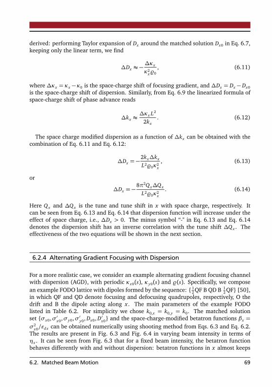
derived: performing Taylor expansion of Dx around the matched solution Dx0 in Eq. 6.7,keeping only the linear term, we find
∆Dx ≈ −∆κx
κ2x%0
, (6.11)
where ∆κx = κx −κ0 is the space-charge shift of focusing gradient, and ∆Dx = Dx − Dx0
is the space-charge shift of dispersion. Similarly, from Eq. 6.9 the linearized formula ofspace-charge shift of phase advance reads
∆kx ≈∆κx L2
2kx. (6.12)
The space charge modified dispersion as a function of ∆kx can be obtained with thecombination of Eq. 6.11 and Eq. 6.12:
∆Dx = −2kx∆kx
L2%0κ2x
, (6.13)
or
∆Dx = −8π2Q x∆Q x
L2%0κ2x
. (6.14)
Here Q x and ∆Q x is the tune and tune shift in x with space charge, respectively. Itcan be seen from Eq. 6.13 and Eq. 6.14 that dispersion function will increase under theeffect of space charge, i.e., ∆Dx > 0. The minus symbol “-" in Eq. 6.13 and Eq. 6.14denotes the dispersion shift has an inverse correlation with the tune shift ∆Q x . Theeffectiveness of the two equations will be shown in the next section.
6.2.4 Alternating Gradient Focusing with Dispersion
For a more realistic case, we consider an example alternating gradient focusing channelwith dispersion (AGD), with periodic κx0(s), κy0(s) and %(s). Specifically, we composean example FODO lattice with dipoles formed by the sequence: 1
2 QF B QD B 12 QF [50],
in which QF and QD denote focusing and defocusing quadrupoles, respectively, O thedrift and B the dipole acting along x . The main parameters of the example FODOlisted in Table 6.2. For simplicity we chose k0,x = k0,y = k0. The matched solutionset σx0,σ′x0,σy0,σ′y0, Dx0, D′x0 and the space-charge-modified betatron functions βx =σ2
x0/εd x can be obtained numerically using shooting method from Eqs. 6.3 and Eq. 6.2.The results are present in Fig. 6.3 and Fig. 6.4 in varying beam intensity in terms ofηx . It can be seen from Fig. 6.3 that for a fixed beam intensity, the betatron functionbehaves differently with and without dispersion: betatron functions in x almost keeps
6.2. Matched Beam Motion 69

Table 6.2.: Main parameters of the example AGD
Parameters [unit] Symbols Values
Length of the AGD [m] L 18.0Length of QF [m] l f 4.0Length of QD [m] ld 4.0Length of dipoles [m] lB 2.618Length of drift [m] lo 1.191Radius of curvature [m] %0 10.0Generalized emittance on x [mm mrad] εd x 10.0Generalized emittance on y [mm mrad] εd y 10.0rms momentum spread σδ 0.002
unchanged, but changes dramatically in y, since the dispersion breaks the symmetricproperty.
Fig.3 presents the results of space-charge-modified dispersion for AGD using Eq. 6.2,compared with the results for CFD using Eq. 6.7 and the approximated results usingscaling law of Eq. 6.14. It can be seen that results from scaling law (dashed line inFig. 6.4) is equal approximately to the average value of the dispersion functions in AGD(dotted line in Fig. 6.4) within in the range of moderate space charge (η≤ 0.2).
6.2.5 RMS-Matched Distribution
The generalized envelope equation of Eq. 6.2 and Eq. 6.3 based on the invariant gen-eralized emittance εd x and εd y are often employed to investigate beam dynamics withspace charge and dispersion [33, 34]. In PIC simulations of beam dynamics in circularaccelerators, the effect of dispersion complicates the beam behavior and the dispersiontends to be difficult to be separated [34]. In this subsection, we introduce a methodon how to generate the transverse particle distribution, which is matched to both SpaceCharge and Dispersion in the rms sense (called “SCD distribution”), and can be usedin PIC simulations for a bent lattice. A major advantage of the SCD distribution is thatthe generalized rms emittance εd x , εd y are invariant, and σx and σδDx can be detectedseparately from the total beam size X in the simulation.
The SCD distribution can be generated in three steps as follows. At first, the particledistribution (e.g. waterbag, Gaussian or KV) rms-matched to the space charge modifiedlattice functions can be obtained from Eqs. 6.3 under the assumption of zero momen-tum spread. Secondly, space-charge-modified dispersion function and its derivate Dx ,D′x can be obtained from Eq. 6.2. Finally, in order to match the dispersion, coordinatetransformation is performed for each macro-particle used in simulation: x = x + δDx
and x ′ = x ′ + δD′x , Here x and x ′ are the individual macro-particle coordinates beforetransformation, and x and x ′ are the ones after transformation; δ represents the cor-
70 6. Space-Charge Dominated Beam Dynamics in Synchrotrons

0 2 4 6 8 10 12 14 16 18
s[m]
10
15
20
25
30
35
βx[m
]
ηx = 0.0, σδ = 0.2%
ηx = 0.1, σδ = 0.2%
ηx = 0.2, σδ = 0.2%
ηx = 0.0, σδ = 0.0
ηx = 0.1, σδ = 0.0
ηx = 0.2, σδ = 0.0
0 2 4 6 8 10 12 14 16 18
s[m]
10
15
20
25
30
35
40
45
βy[m
]
ηx = 0.0, σδ = 0.2%
ηx = 0.1, σδ = 0.2%
ηx = 0.2, σδ = 0.2%
ηx = 0.0, σδ = 0.0
ηx = 0.1, σδ = 0.0
ηx = 0.2, σδ = 0.0
Figure 6.3.: Space-charge-modified betatron functions in x (left plot) and y (right plot)with (solid line) and without (dashed line) dispersion effect in one AGD peri-odic cell, for ηx = 0.0, 0.1,0.2.
0 2 4 6 8 10 12 14 16 18
s[m]
6
8
10
12
14
16
18
Dx[m
]
ηx = 0.0
ηx = 0.1
ηx = 0.2
Figure 6.4.: Space-charge-modified dispersion functions in one AGD periodic cell (solidline) with varying beam current (ηx = 0.0, 0.1,0.2.), compared with the dis-persion in CFD case (dotted line) and the approximated dispersion evaluatedfrom the scaling law (dashed line).
6.2. Matched Beam Motion 71

Figure 6.5.: An example of the SCD distribution (red) in x − x ′ phase space (a) andx − y real space (b), generated from a KV distribution (blue) by coordinatetransformation. εd x = 10.0 mm mrad, σδ = 1.0× 10⁻³.
responding individual fractional momentum deviation of each macro-particle. In theabove process, the coordinates x , x ′ of all macro-particles form the betatron beam sizeσx =
p
⟨ x⟩2 and the generalized rms emittance εx =Æ
⟨ x2⟩⟨ x ′2⟩ − ⟨ x x ′⟩2 in x and canbe tracked in the simulation. For the cases with moderate space charge, εd x stays con-stant in the simulation. The coordinates x , x ′ form the total rms beam size X and thetotal rms emittance εx . Since the effect of dispersion is assumed acted only in x , in yno coordinate transformation is needed.
It is worth pointing out that the SCD distribution is dependent on the momentumspread distribution, and thus is not strictly self-consistent with space charge, since thespace charge force becomes nonlinear during the process of coordinate transformation.Nevertheless, the relation in Eq. F.4 indicates that the distribution generated by theabove procedure is rms-matched to the external focusing force, the space charge andthe dispersion. As long as the space charge is moderate, which is typical in most circularmachines [4], the total rms beam size X and Y will not be dramatically influenced bythe nonlinear space charge force, indicating that the generalized rms emittance εd x andεd y stays constant.
6.3 Mismatched Beam Motion
6.3.1 Dispersion Matching
As introduced in section 1, for a matched beam characterized with σx0,σy0, Dx0, thetotal matched rms beam size X0(s) consists of two independent parts: betatron beamsize σx0(s) and dispersion beam size σδDx0(s) satisfying the relation
X 20 = σ
2x0 +σ
2δD2
x0, (6.15)
72 6. Space-Charge Dominated Beam Dynamics in Synchrotrons
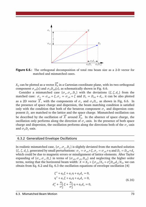
X
X0σx0
σδDx0
σx
σδDx
ξ
σδdx
Figure 6.6.: The orthogonal decomposition of total rms beam size as a 2-D vector formatched and mismatched cases.
X0 can be plotted as a vector−→X0 in a Cartesian coordinate plane, with its two orthogonal
component σx0(s) and σδDx0(s), as schematically shown in Fig. 6.6.Consider a mismatched case σx ,σy , Dx with the deviations ξ,ζ, dx from the
matched case: σx = σx0 + ξ,σy = σy0 + ζ and Dx = Dx0 + dx , it can be also plotted
as a 2D vector−→X , with the components of σx and σδDx , as shown in Fig, 6.6. In
the presence of space charge and dispersion, the beam matching condition is satisfiedonly with the condition that both of the betatron component σx and dispersion com-ponent Dx are matched to the lattice and the space charge. Mismatched oscillation canbe described by the oscillation of
−→X around
−→X0. In the absence of space charge, the
oscillation only performs along the direction of σx -axis. In the presence of both spacecharge and dispersion, the oscillation performs along the directions both of the σx -axisand σδDx -axis.
6.3.2 Generalized Envelope Oscillations
In realistic mismatched case, σx ,σy , Dx is slightly deviated from the matched solutionξ, ζ, dx, generated by small perturbations: σx = σx0+ξ,σy = σy0+η and Dx = Dx0+dx
which could be due to magnetic errors or misalignment of lattice elements. After Taylorexpanding of σx ,σy , Dx in terms of σx0,σy0, Dx0 and neglecting the higher orderterms, noting that the horizontal beam width: X = X0 + ξσx0/X0 +σ2
δDx0dx/X0, we can
obtain from Eq. 6.2 and Eq. 6.3 the oscillation equations of envelope oscillation [4]
ξ′′ + a0ξ+ a1η+ a2dx = 0,
η′′ + a1ξ+ a3η+ a4dx = 0,
d ′′x +a2
σ2δ
ξ+a4
σ2δ
η+ a5dx = 0,(6.16)
6.3. Mismatched Beam Motion 73
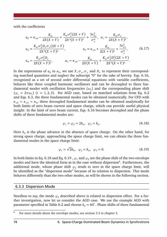
with the coefficients
a0 = κx0 −Ksc
2X (X + Y )+
Kscσ2x (2X + Y )
2X 3(X + Y )2+
3ε2d x
σ4x
, a1 =Kscσx
2X (X + Y )2,
a2 =Kscσ
2δDxσx (2X + Y )
2X 3(X + Y )2, a3 = κy0 +
Ksc
2(X + Y )2+
3ε2d y
σ4y
,
a4 =Kscσ
2δDx
2X (X + Y )2, a5 = κx0 −
Ksc
2X (X + Y )+
Kscσ2δD2
x (2X + Y )
2X 3(X + Y )2.
(6.17)
In the expressions of a0 to a5, we use X ,σx ,σy and Dx to represent their correspond-ing matched quantities and neglect the subscript “0” for the sake of brevity. Eqs. 6.16,recognized as a set of second order differential equations with variable coefficients,behaves like three coupled harmonic oscillators and can be decoupled to three fun-damental modes with oscillation frequencies ωi and the corresponding phase shiftϕi = 2πωi (i = 1,2, 3). For AGD case, based on matched solutions from Eq. 6.2and Eqs. 6.3, the three fundamental modes can be obtained numerically. For CFD withκx0 = κy0 = κ0, three decoupled fundamental modes can be obtained analytically forboth limits of zero beam current and space charge, which can provide useful physicalinsight: In the limit of zero beam current, Eqs. 6.16 becomes decoupled and the phaseshifts of three fundamental modes are:
ϕ1 = ϕ2 = 2k0, ϕ3 = k0. (6.18)
Here k0 is the phase advance in the absence of space charge. On the other hand, forstrong space charge, approaching the space charge limit, we can obtain the three fun-damental modes in the space charge limit:
ϕ1 =p
2k0, ϕ2 = k0, ϕ3 = 0. (6.19)
In both limits in Eq. 6.18 and Eq. 6.19 , ϕ1 and ϕ2 are the phase shifs of the two envelopemodes and have the identical form as in the case without dispersion6. Furthermore, theadditional mode, whose phase shift ϕ3 tends to zero in the space charge limit, willbe identified as the “dispersion mode” because of its relation to dispersion. This modebehaves differently than the two other modes, as will be shown in the following section.
6.3.3 Dispersion Mode
Needless to say, the mode ϕ3 described above is related to dispersion effect. For a fur-ther investigation, now let us consider the AGD case. We use the example AGD withparameter specified in Table 6.2 and choose k0 = 60. Phase shifts of three fundamental
6 For more details about the envelope modes, see section 3.3 in chapter 3.
74 6. Space-Charge Dominated Beam Dynamics in Synchrotrons
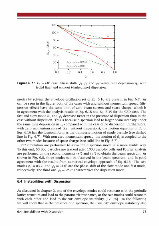
0.0 0.2 0.4 0.6 0.8 1.0ηx
0
20
40
60
80
100
120
φ1,2,3[deg]
φ1
φ2
φ3φ1,2,3 (σδ = 0.2%)
φ1,2,3 (σδ = 0.0)
Figure 6.7.: k0 = 60 case: Phase shifts ϕ1,ϕ2 and ϕ3 versus tune depression ηx with(solid line) and without (dashed line) dispersion.
modes by solving the envelope oscillation set of Eq. 6.16 are present in Fig. 6.7. Ascan be seen in the figure, both of the cases with and without momentum spread (dis-persion effect) have the same limit of zero beam current and space charge, which isin agreement with the analysis results in Eq. 6.18 and Eq. 6.19 for the CFD case. Thefast and slow mode ϕ1 and ϕ2 decrease faster in the presence of dispersion than in thecase without dispersion. This is because dispersion lead to larger beam intensity underthe same tune depression in x , compared with the case of no dispersion. Furthermore,with zero momentum spread (i.e. without dispersion), the motion equation of dx inEqs. 6.16 has the identical form as the transverse motion of single particle (see dashedline in Fig. 6.7). With non-zero momentum spread, the motion of dx is coupled to theother two modes because of space charge (see solid line in Fig. 6.7).
PIC simulation are performed to show the dispersion mode in a more visible way.To this end, 50 000 particles are tracked after 1000 periodic cells and Fourier analysisare performed on the second moments ⟨x2⟩ and ⟨y2⟩ to obtain the beam spectrum. Asshown in Fig. 6.8, three modes can be observed in the beam spectrum, and in goodagreement with the results from numerical envelope approach of Eq. 6.16. The twomodes ϕ1 = 83.2 and ϕ2 = 94.6 are the phase shift of the slow mode and fast mode,respectively. The third one ϕ3 = 52.7 characterizes the dispersion mode.
6.4 Instabilities with Dispersion
As discussed in chapter 3, one of the envelope modes could resonate with the periodiclattice structure and lead to the parametric resonance, or the two modes could resonatewith each other and lead to the 90 envelope instability [17, 76]. In the followingwe will show that in the presence of dispersion, the usual 90 envelope instability also
6.4. Instabilities with Dispersion 75

Figure 6.8.: Beam spectrum of ⟨x2⟩ (blue) and ⟨y2⟩ (green) in the presence of disper-sion and space charge from PIC simulation, compared with the results of fastmode, slow mode and dispersion mode calculated from envelope oscillationequation (dashed red line) of the example AGD with k0 = 60
exists, with its stopbands slightly shifted, compared with the case without dispersion.Moreover, in the presence of dispersion, the identified dispersion mode could also res-onate with other two envelope modes under certain beam current intensity in periodiclattice, and can induce the recently discovered dispersion-induced instability [4].
Analogy to the treatment introduced in chater 3, the stability analysis in the presenceof dispersion can be performed by integrating Eqs. 6.16 over one periodic focusing cell(from m to m+ 1)
ζm+1 = Mζm, (6.20)
where M is the map for the perturbation vector ζ = (ξ,ξ′,η,η′, dx , d ′x ) over one cell. Asσx ,σ′x ,σy ,σ′y , Dx , D′x in Eq. 6.2 and Eqs. 6.3 follow the Hamiltonian of Eq. F.1, the sixeigenvalues of M : λi = |λi |eiϕi (i = 1, 2, . . . , 6) exist only as reciprocal or as conjugatein three pairs: λ1,λ∗1, λ2,λ∗2, λ3,λ∗3. Moreover, taking each oscillation mode inspace charge limits in Eq. 6.19 as reference, we can select a suitable set of phase shiftsϕ1,ϕ2,ϕ3 with corresponding moduli |λ1|, |λ2|, |λ3| representing fast mode, slowmode and the dispersion mode respectively, to fully characterize the beam oscillationwithout loss of generality. One of the three moduli larger than unity can be used asinstability growth factor. For detailed analysis of the movement of the six eigenvaluesin the presence of dispersion under different beam intensity see Appendix F.
Taking the AGD lattice with parameters listed in Table 6.2 as an example withk0,x = k0,y = k0, the numerical integration of Eq. 6.20 is performed and the resultsof ϕ1,ϕ2,ϕ3 are shown in Fig. 6.9, Fig. 6.10 and Fig. 6.11 for the three representativecases of k0 = 90, k0 = 120 and k0 = 130 respectively, compared with the correspond-ing case of zero momentum spread. Fig. 6.9 shows a stable case with growth factorsare equal to unit (not shown here), and the three modes have a similar behavior as thecase of k0 = 60 in Fig. 6.7. In contrary, Fig. 6.10 and Fig. 6.11 are shown with growth
76 6. Space-Charge Dominated Beam Dynamics in Synchrotrons
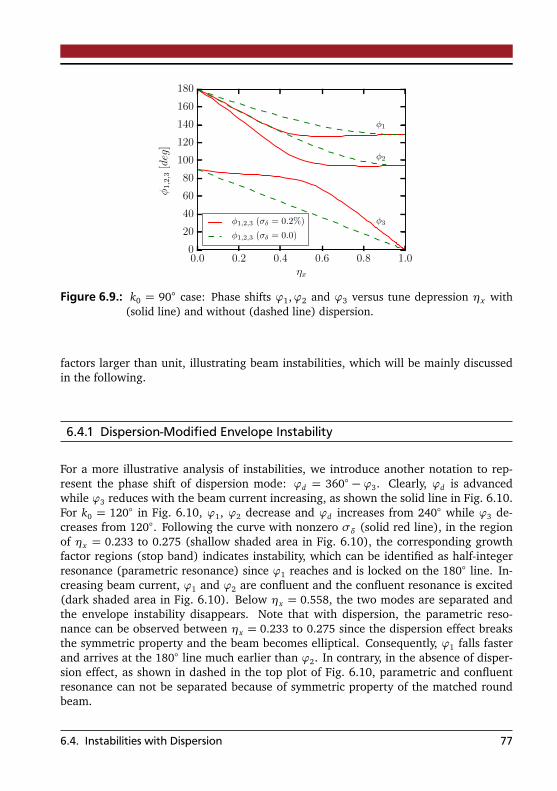
0.0 0.2 0.4 0.6 0.8 1.0ηx
0
20
40
60
80
100
120
140
160
180
φ1,2,3[deg]
φ1
φ2
φ3φ1,2,3 (σδ = 0.2%)
φ1,2,3 (σδ = 0.0)
Figure 6.9.: k0 = 90 case: Phase shifts ϕ1,ϕ2 and ϕ3 versus tune depression ηx with(solid line) and without (dashed line) dispersion.
factors larger than unit, illustrating beam instabilities, which will be mainly discussedin the following.
6.4.1 Dispersion-Modified Envelope Instability
For a more illustrative analysis of instabilities, we introduce another notation to rep-resent the phase shift of dispersion mode: ϕd = 360 − ϕ3. Clearly, ϕd is advancedwhile ϕ3 reduces with the beam current increasing, as shown the solid line in Fig. 6.10.For k0 = 120 in Fig. 6.10, ϕ1, ϕ2 decrease and ϕd increases from 240 while ϕ3 de-creases from 120. Following the curve with nonzero σδ (solid red line), in the regionof ηx = 0.233 to 0.275 (shallow shaded area in Fig. 6.10), the corresponding growthfactor regions (stop band) indicates instability, which can be identified as half-integerresonance (parametric resonance) since ϕ1 reaches and is locked on the 180 line. In-creasing beam current, ϕ1 and ϕ2 are confluent and the confluent resonance is excited(dark shaded area in Fig. 6.10). Below ηx = 0.558, the two modes are separated andthe envelope instability disappears. Note that with dispersion, the parametric reso-nance can be observed between ηx = 0.233 to 0.275 since the dispersion effect breaksthe symmetric property and the beam becomes elliptical. Consequently, ϕ1 falls fasterand arrives at the 180 line much earlier than ϕ2. In contrary, in the absence of disper-sion effect, as shown in dashed in the top plot of Fig. 6.10, parametric and confluentresonance can not be separated because of symmetric property of the matched roundbeam.
6.4. Instabilities with Dispersion 77

0
50
100
150
200
250
300
350
φ1,2,3,d[deg]
180line
φ3
φd = 360 − φ3
φ1
φ2
φ1,2,3,d (σδ = 0.2%)
φ1,2,3,d (σδ = 0.0%)
0.0 0.2 0.4 0.6 0.8 1.0ηx
1.0
1.1
1.2
1.3
1.4
1.5
|λ|
parametric
confluent
confluent& parametric
φ1,2,3,d (σδ = 0.2%)
φ1,2,3,d (σδ = 0.0%)
λ (σδ = 0.2%)
λ (σδ = 0.0)
Figure 6.10.: k0 = 120 case. Upper: Phase shifts ϕ1, ϕ2, ϕ3 and ϕd versus tune depres-sion ηx , with (solid red) and without (green dashed) dispersion; Lower:Growth factor |λ| versus ηx with (red) and without (green) dispersion.(Shaded area denotes the stop band of the envelope instability modifiedby dispersion: parametric resonance (shallow) and confluent resonance(dark)).
78 6. Space-Charge Dominated Beam Dynamics in Synchrotrons

6.4.2 Dispersion-Induced Envelope Instability
The instability induced by dispersion is illustrated in Fig. 6.11 for k0 = 130, where dis-persion mode becomes unstable. The stop band from ηx = 0.092 to 0.153 (shade areain Fig. 6.11) indicates instability (the corresponding simulation results of the emittancegrowth and phase space evaluation shown in Fig. 6.11 will be discussed later). Since inthis region, confluence occurs between the dispersion mode ϕd and the slow mode ϕ1
(solid curve in the top plot of Fig. 6.11), this instability is induced by periodic focusingand dispersion and can be related to a resonance between the two modes. For com-pleteness, phase shifts of ϕ1 and ϕ2 in the absence of momentum spread are plotted forcomparison in the top plot of Fig. 6.11.
A criteria for the occurrence of dispersion-induced instability can be given based onthe following analyses: in Fig. 6.11, ϕ0
1 = 260, ϕ0d = 240 and ϕ0
d < ϕ01 (here the
superscript “0" denotes values in the absence of space charge). This is different from thecase in Fig. 6.10, in which ϕ0
1 = ϕ02 = ϕ
0d = 240 and no confluence occurs between ϕ1
and ϕd . These analyses show that only if ϕ01 > ϕ
0d , e.g. 2k0 > 360− k0, or k0 > 120, ϕ1
and ϕd can be confluent, and hence the dispersion-induced instability occurs. In otherwords, for a lattice of k0,x = k0,y = k0, only with k0 > 120 satisfied, the dispersion-induced instability may occur within a certain beam current range. For a more physicalinterpretation, the extended envelope oscillation system including dispersion containsthree fundamental modes. The mode of dispersion oscillation (ϕd or ϕ3) behaves, tosome extend, like a single particle as Eq. 6.2 lacks the emittance term, which is differentfrom the two other modes ϕ1 and ϕ2. For a lattice of k0,x = k0,y = k0 only with k0 > 120,ϕd -mode may resonate with ϕ1-mode in a certain beam current range, and induce thebeam instability with the periodic focusing. For completeness, it can be observed thatthe usual 90 envelope instability from parametric and confluent resonances exist belowηx = 0.277, which is similar to the case of k0 = 120 in Fig. 6.10.
The criteria above can be extended to a more general case. Let us consider a periodiclattice with k0,x > k0,y (An example with k0,x = 130, k0,y = 120 is shown in Fig. 6.12).With increasing beam current the fast mode ϕ1 and the slow mode ϕ2 decrease from2k0,x and 2k0,y respectively, while ϕd increases from 360 − k0,x . Therefore, ϕ1 can beconfluent with ϕd when satisfying 2k0,x > 360 − k0,x , e.g.
k0,x > 120. (6.21)
Therefore the dispersion-induced envelope instability can be named “120 dispersioninstability”, in contrast to the usual envelope instability related to k0,x ,y > 90.
Two main properties of the 120 dispersion instability are briefly demonstrated infollowing. Firstly, in the general case for k0,x 6= k0,y , as shown in Fig. 6.12 withk0,x = 130, k0,y = 120 as an example, although ϕ2 intersects with ϕd at ηx = 0.0384,no confluence between them. Confluence only occurs between ϕ1 and ϕd . These obser-vations indicate one important feature of dispersion induced instability: it occurs onlywithin the dispersion acting plane (in the context it is in x), in which space charge effect,
6.4. Instabilities with Dispersion 79
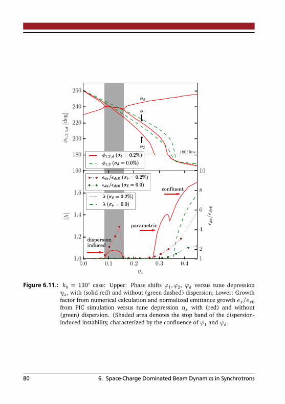
160
180
200
220
240
260
φ1,2,3,d[deg]
180line
φd
φ1
φ2
φ1,2,d (σδ = 0.2%)
φ1,2 (σδ = 0.0%)
0.0 0.1 0.2 0.3 0.4ηx
1.0
1.2
1.4
1.6
|λ|
dispersioninduced
parametric
confluentλ (σδ = 0.2%)
λ (σδ = 0.0)
1
2
4
6
8
10
ǫ dx/ǫ
dx0
φ1,2,d (σδ = 0.2%)
φ1,2 (σδ = 0.0%)
λ (σδ = 0.2%)
λ (σδ = 0.0)
ǫdx/ǫdx0 (σδ = 0.2%)
ǫdx/ǫdx0 (σδ = 0.0)
ǫdx/ǫdx0 (σδ = 0.2%)
ǫdx/ǫdx0 (σδ = 0.0)
Figure 6.11.: k0 = 130 case: Upper: Phase shifts ϕ1,ϕ2, ϕd versus tune depressionηx , with (solid red) and without (green dashed) dispersion; Lower: Growthfactor from numerical calculation and normalized emittance growth εx/εx0from PIC simulation versus tune depression ηx with (red) and without(green) dispersion. (Shaded area denotes the stop band of the dispersion-induced instability, characterized by the confluence of ϕ1 and ϕd .
80 6. Space-Charge Dominated Beam Dynamics in Synchrotrons
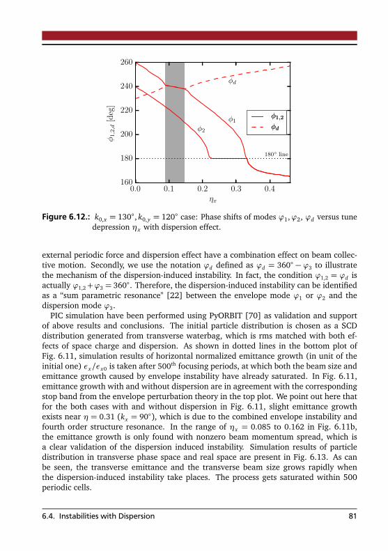
0.0 0.1 0.2 0.3 0.4ηx
160
180
200
220
240
260
φ1,2,d[deg]
180 line
φd
φ1
φ2
φ1,2
φd
φ1,2
φd
Figure 6.12.: k0,x = 130, k0,y = 120 case: Phase shifts of modes ϕ1,ϕ2, ϕd versus tunedepression ηx with dispersion effect.
external periodic force and dispersion effect have a combination effect on beam collec-tive motion. Secondly, we use the notation ϕd defined as ϕd = 360 − ϕ3 to illustratethe mechanism of the dispersion-induced instability. In fact, the condition ϕ1,2 = ϕd isactually ϕ1,2+ϕ3 = 360. Therefore, the dispersion-induced instability can be identifiedas a “sum parametric resonance" [22] between the envelope mode ϕ1 or ϕ2 and thedispersion mode ϕ3.
PIC simulation have been performed using PyORBIT [70] as validation and supportof above results and conclusions. The initial particle distribution is chosen as a SCDdistribution generated from transverse waterbag, which is rms matched with both ef-fects of space charge and dispersion. As shown in dotted lines in the bottom plot ofFig. 6.11, simulation results of horizontal normalized emittance growth (in unit of theinitial one) εx/εx0 is taken after 500th focusing periods, at which both the beam size andemittance growth caused by envelope instability have already saturated. In Fig. 6.11,emittance growth with and without dispersion are in agreement with the correspondingstop band from the envelope perturbation theory in the top plot. We point out here thatfor the both cases with and without dispersion in Fig. 6.11, slight emittance growthexists near η = 0.31 (kx = 90), which is due to the combined envelope instability andfourth order structure resonance. In the range of ηx = 0.085 to 0.162 in Fig. 6.11b,the emittance growth is only found with nonzero beam momentum spread, which isa clear validation of the dispersion induced instability. Simulation results of particledistribution in transverse phase space and real space are present in Fig. 6.13. As canbe seen, the transverse emittance and the transverse beam size grows rapidly whenthe dispersion-induced instability take places. The process gets saturated within 500periodic cells.
6.4. Instabilities with Dispersion 81

Figure 6.13.: PIC simulation results of particle distribution evolution in transverse phasespace and real space for k0 = 130 and ηx = 0.885 (kx = 115).
82 6. Space-Charge Dominated Beam Dynamics in Synchrotrons

7 Space Charge Limitation for BunchCompression in Synchrotrons
In this chapter, we investigate the 3-D beam behavior during bunch compression in high-current synchrotrons, with an example case in GSI SIS-18. The transverse envelopeequations introduced in previous chapter are coupled with the longitudinal envelopeequation. Based on the coupled longitudinal-transverse envelope equation set and alsoparticle-in-cell (PIC) simulations, the mechanism of the coherent beam instability andthe incoherent single particle resonance related to the enhanced space charge duringbunch compression are analyzed in detailed.
Section 7.1 presents the theoretical model of the coupled longitudinal-transverse en-velope equation set and PIC simulations of bunch compression. In section 7.2, as anapplication of the two approaches to describe the bunch compression in SIS-18, wesolve numerically the coupled envelope equation set with a set of typical beam pa-rameters, in comparison with PIC simulation results. At last, in section 7.3 two majorspace-charge limits for bunch compression in SIS-18 with phase advance crossing theresonance conditions related to 90 and 120 line are investigated. The competingmechanisms of the fourth-order resonance, envelope instability and dispersion-inducedinstability during bunch compression are demonstrated.
7.1 Two Approaches of Bunch Compression
The envelope approach and PIC simulations are two commonly used methods for bunchcompression study. Based on the longitudinal envelope equation introduced in section3.4, the required rf voltage for bunch rotation can be calculated [45]. The transversespace-charge tune shift during bunch compression can be obtained by solving the trans-verse envelope equation set [46]. This section introduces the coupled longitudinal-transverse envelope equation set, and briefly discusses several considerations for per-forming simulations of bunch compression. In the following we assume x and y forthe horizontal and vertical directions, and z the longitudinal one; s is distance as inde-pendent variable. k0,x ,y , kx ,y are the phase advances per focusing cell without and withspace charge, respectively.
83
7.1.1 Coupled Longitudinal-Transverse Envelope System
Let us start with a bunched beam with parabolic distribution in the longitudinal plane,for which the space charge forces are linear in z. The corresponding longitudinal enve-lope equation including space charge takes the form1
z′′m +κz0zm −KL
z2m
−ε2
L
z3m
= 0. (7.1)
Here, zm is the half length of the bunch, and κz0 is the linearized external rf focusingforce defined in Eq. 3.36. Vr f is the rf voltage required for fast bunch compression,Zq and Am0 the charge and the mass of the particle, h the harmonic number, η the slipfactor, c the speed of light, β and γ the relativistic factors, and R the average radius of thesynchrotron. The linearized external focusing gradient modified by longitudinal spacecharge is κz = κz0 − KL/z
3m, with the longitudinal perveance KL = 3gN Z2rp/(2β2γ5A);
the geometry factor g = 0.5+ 2 ln(Rp/Rb) (Rp and Rb are the radii of the beam pipe andthe beam, respectively); N the number of particles in the bunch; rp the classical protonradius and η the slip factor. εL is the longitudinal emittance, defined as
εL = |η|zmδ0, (7.2)
in which δ0 is the momentum spread at the center of the bunch δ0 = δ(z = 0), as shownin Fig. 7.1. Physically, εL denotes the area in longitudinal phase space, which is constantwithout acceleration. During compression, the ellipse of the longitudinal emittancerotates and becomes tilted, and the maximum momentum spread of the bunch δ can beexpress as δ2
m = δ2+δ2
0. Here, δ is the momentum spread of the particles at the edge ofthe bunch, and δ0 the maximum momentum spread at the bunch center.
The rf voltage required for bunch compression can be derived by integratingEq. 7.1 [45],
∫
d z′m
2
2
+κz0
∫
zmdzm − KL
∫
dzm
z2m
− ε2L
∫
dzm
z3m
= 0, (7.3)
from which we obtain a longitudinal invariance,
IL =z′2m2+κz0
2z2
m +KL
zm+ε2
L
2z2m
. (7.4)
1 For more details of the longitudinal envelope equations and the parabolic distribution, see sec-tion 3.4.
84 7. Space Charge Limitation for Bunch Compression in Synchrotrons

Figure 7.1.: Definition of parameters in longitudinal phase space. z denotes the longitu-dinal direction, and δ =∆p/p0 is the relative momentum deviation.
It is convenient to introduce a compression factor χ (χ ≤ 1), defined as
zm, f = χzm,i , (7.5)
in which zm, f and zm,i denote the initial and final longitudinal envelope during bunchcompression. For the ideal bunch compression with a parabolic distribution and linearlongitudinal space charge force, the longitudinal emittance εL remains invariant, andthe final momentum spread results as δm, f obeys δm, f =
δm,iχ .
Substituting zm,i , zm, f and δm,i , δm, f into the invariant emittance of Eq. 7.3, and usingthe compression factor χ, we can obtain
κz0 = |η|δm,i
zm,iχ
2
1+2KLzm, f
ε2L(1+χ)
. (7.6)
The required rf voltage for bunch compression can be derived via substituting Eq. 7.6into Eq. 3.36,
Vr f = |η|δm,i
zm,iχ
2
1+2KLzm,iχ
ε2L(1+χ)
2πR2γβ2Am0c2
Zqhη. (7.7)
It can be seen from Eq. 7.7 that the rf voltage for the bunch compression is a function ofthe initial bunch length zm,i , momentum spread δm,i and the compression factor χ. Vr f
is inversely proportional to the bunch compression factor χ, or the final bunch lengthzm, f .
7.1. Two Approaches of Bunch Compression 85

Since during bunch compression the synchrotron phase are chosen to zero, the syn-chrotron frequency can be written as (see, for example, in Ref. [50])
ωs =
√
√
√ZqhVr f |η|2πR2Am0γ
. (7.8)
Since bunch compression are performed by one quarter synchrotron motion, the turnsneeded for compression are
n=14ω0
ωs, (7.9)
where ω0 = β0c/R is the revolution frequency. Note that in Eq. 7.8 and Eq. 7.9 the lon-gitudinal space charge is ignored. For the parameters in the present study, longitudinalspace charge is sufficiently small that Eq. 7.9 can be used to calculate the turns requiredfor bunch compression.
The longitudinal envelope equation of Eq. 7.1 can be used to describe the longitudinalbeam dynamics and calculate the required rf voltage in bunch compression. By includ-ing the space-charge modified dispersion, the envelope equations become a useful toolto study the transverse collective motion in synchrotrons. During bunch compression,both space charge and its effect on dispersion are increasing. Therefore, the trans-verse envelope equation should be coupled with the longitudinal equation to give a fulldescription of the beam dynamics of bunch compression.
There are several considerations when applying the coupled set of equations on bunchcompression. The first consideration is that even for fast bunch rotation the synchrotronfrequency is much smaller than the transverse one, which means space charge is increas-ing “adiabatically” for the transverse motion. Therefore, it is reasonable to assume thatthe beam has sufficient time to remain matched to the transverse lattice during bunchcompression. The second point is that the variable zm in the longitudinal equationshould be transformed to its corresponding rms quantity σz , in order to calculate therms momentum spread and dispersion. For parabolic distributions the transformationis performed by σz =
p5zm. Based on above considerations, the coupled longitudinal-
transverse set of equations takes the form
z′′m +
κz0zm −KL
z3m
zm −ε2
z
z3m
= 0,
σ′′x +
κx0 −Ksc
2X (X + Y )
σx −ε2
d x
σ3x
= 0,
σ′′y +
κy0 −Ksc
2Y (X + Y )
σy −ε2
d y
σ3y
= 0,
D′′x +
κx0 −Ksc
2X (X + Y )
Dx =1%(s)
,
(7.10)
86 7. Space Charge Limitation for Bunch Compression in Synchrotrons
with the coupled relations
X =q
σ2x +σ
2δD2
x , Y = σy , (7.11)
and
σδ =
√
√
√
σ′zη
2
+
εz
ησz
2
, σz =p
5zm. (7.12)
Here, κx0,y0 and κz0 are the linearized external focusing gradients in transverse andlongitudinal plane, respectively. σx ,y denote the transverse rms betatron beam size;X and Y the transverse rms total beam size with dispersion; σδ the rms momentumspread; σz the rms half bunch length; εd x ,d y the generalized transverse rms emittancedefined in Ref. [29], and εz the longitudinal rms emittance defined in Eq. 7.2.
7.1.2 PIC Simulations
A major consideration of PIC-simulation of bunch compression is the treatment of spacecharge. For typical parameters of bunch compression in synchrotrons, the bunch lengthafter bunch compression is usually in the order of several meters, and much largerthan the transverse beam size, which is in the order of centimeters or less. Therefore,as introduced in section 4.2, the treatment of space charge in the simulation can besplit into a 1-D longitudinal calculation and a 2-D transverse calculation, which is oftenreferred to as “2.5-D” in literature (see, for example in Ref. [70]).
Another consideration is the generation of the initial particle distribution. The lon-gitudinal one can be chosen as parabolic, which is - at least initially - a self-consistentmodel. In order to compare with the envelope approach, the external longitudinal rffocusing force is chosen to be linear. In the transverse plane, the initial distribution ischosen as a Gaussian (truncated at 3σ, here σ is the standard deviation).
For bunched beams different longitudinal positions experience different transversespace charge forces, and thus different space-charge modified lattice functions. In thesimulation performed here, we adopt the approximation that the initial bunched beamis transversely rms-matched with lattice functions modified by space charge at the longi-tudinal beam center. The beam current at the center of a parabolic bunch takes the formI = %L0β0c = 3N Zqβ0c/(4zm). Here N is the number of particles in the bunched beamand %L0 = 3Nq/(4zm) the linear charge density at the beam center. Substituting thebeam current into Eq. 7.10, the matched rms beam size can be calculated numerically.
7.2 An Example of Bunch Compression in the SIS-18
The lattice of the SIS-18 consists of 12 periodic cells formed by the sequence QF B QDB, in which QF and QD denote focusing and defocussing quadrupoles respectively, andB represents the dipoles. The assumed type of ion is U73+. The related parameters for
7.2. An Example of Bunch Compression in the SIS-18 87
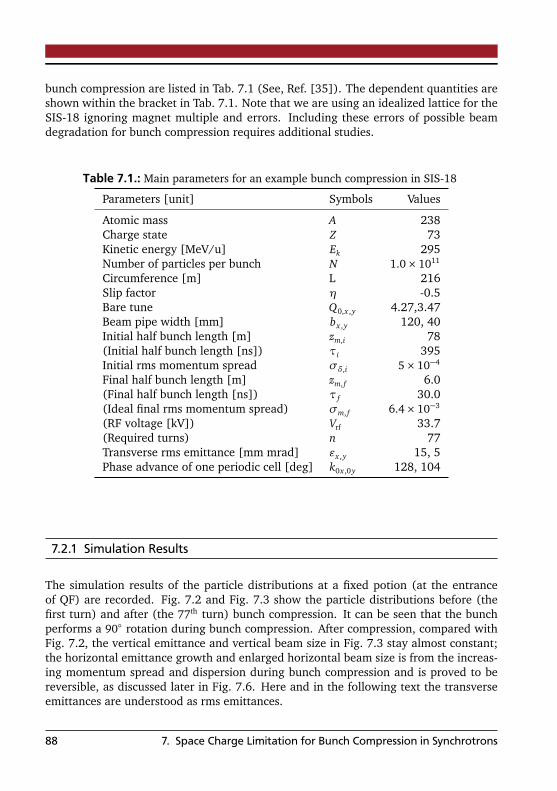
bunch compression are listed in Tab. 7.1 (See, Ref. [35]). The dependent quantities areshown within the bracket in Tab. 7.1. Note that we are using an idealized lattice for theSIS-18 ignoring magnet multiple and errors. Including these errors of possible beamdegradation for bunch compression requires additional studies.
Table 7.1.: Main parameters for an example bunch compression in SIS-18
Parameters [unit] Symbols Values
Atomic mass A 238Charge state Z 73Kinetic energy [MeV/u] Ek 295Number of particles per bunch N 1.0× 10¹¹
Circumference [m] L 216Slip factor η -0.5Bare tune Q0,x ,y 4.27,3.47Beam pipe width [mm] bx ,y 120, 40Initial half bunch length [m] zm,i 78(Initial half bunch length [ns]) τi 395Initial rms momentum spread σδ,i 5× 10⁻⁴
Final half bunch length [m] zm, f 6.0(Final half bunch length [ns]) τ f 30.0(Ideal final rms momentum spread) σm, f 6.4× 10⁻³
(RF voltage [kV]) Vrf 33.7(Required turns) n 77Transverse rms emittance [mm mrad] εx ,y 15, 5Phase advance of one periodic cell [deg] k0x ,0y 128, 104
7.2.1 Simulation Results
The simulation results of the particle distributions at a fixed potion (at the entranceof QF) are recorded. Fig. 7.2 and Fig. 7.3 show the particle distributions before (thefirst turn) and after (the 77th turn) bunch compression. It can be seen that the bunchperforms a 90 rotation during bunch compression. After compression, compared withFig. 7.2, the vertical emittance and vertical beam size in Fig. 7.3 stay almost constant;the horizontal emittance growth and enlarged horizontal beam size is from the increas-ing momentum spread and dispersion during bunch compression and is proved to bereversible, as discussed later in Fig. 7.6. Here and in the following text the transverseemittances are understood as rms emittances.
88 7. Space Charge Limitation for Bunch Compression in Synchrotrons
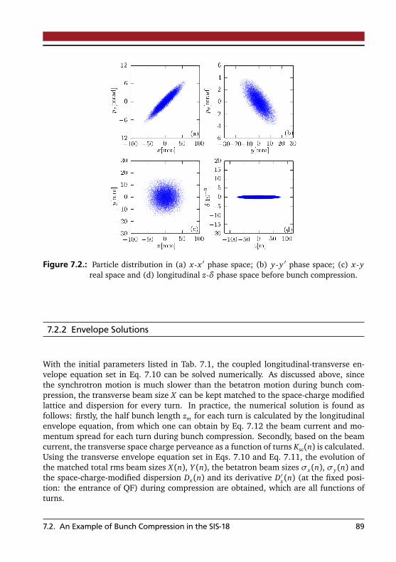
Figure 7.2.: Particle distribution in (a) x-x ′ phase space; (b) y-y ′ phase space; (c) x-yreal space and (d) longitudinal z-δ phase space before bunch compression.
7.2.2 Envelope Solutions
With the initial parameters listed in Tab. 7.1, the coupled longitudinal-transverse en-velope equation set in Eq. 7.10 can be solved numerically. As discussed above, sincethe synchrotron motion is much slower than the betatron motion during bunch com-pression, the transverse beam size X can be kept matched to the space-charge modifiedlattice and dispersion for every turn. In practice, the numerical solution is found asfollows: firstly, the half bunch length zm for each turn is calculated by the longitudinalenvelope equation, from which one can obtain by Eq. 7.12 the beam current and mo-mentum spread for each turn during bunch compression. Secondly, based on the beamcurrent, the transverse space charge perveance as a function of turns Ksc(n) is calculated.Using the transverse envelope equation set in Eqs. 7.10 and Eq. 7.11, the evolution ofthe matched total rms beam sizes X (n), Y (n), the betatron beam sizes σx (n), σy(n) andthe space-charge-modified dispersion Dx (n) and its derivative D′x (n) (at the fixed posi-tion: the entrance of QF) during compression are obtained, which are all functions ofturns.
7.2. An Example of Bunch Compression in the SIS-18 89

Figure 7.3.: Particle distribution in (a) x-x ′ phase space; (b) y-y ′ phase space; (c) x-yreal space and (d) longitudinal z-δ phase space after bunch compression.
7.2.3 Comparison of Simulation and Envelopes
The numerical solutions of bunch length zm are shown in Fig. 7.4 and compared withthe simulation results. It can be seen that the evolution of bunch length during bunchcompression from the envelope approach is almost perfect matched with the simulationresults.
Fig. 7.5 shows the transverse results from the two approaches. The blue solid line andblue dotted line are the transverse rms beam size (X ) and betatron rms beam size (σx )solved from the coupled envelope method. The red solid line and red dotted line are thetransverse rms beam size and betatron rms beam size obtained from the simulation. The
former can be obtained directly by the definition of the rms quantity: X = 1N
N∑
i=1x2
i
1/2,
while the latter is obtained by σx =1N [
N∑
i=1(x i−δi Dx )2]1/2. Here x i denotes the horizontal
offset of the ith macro particle, N the total number of macro particles in the simulationand Dx the space-charge-modified dispersion solved from the envelope approach. It canbe seen from Fig. 7.5 that during bunch compression the total horizontal beam size Xis increasing due to the increasing dispersion, while the betatron beam size σx remainsconstant. The results of transverse beam sizes from the envelope approach agree wellwith the results from PIC simulations.
90 7. Space Charge Limitation for Bunch Compression in Synchrotrons

0 20 40 60 80 100
turns
0
10
20
30
40
50
60
70
80
z m[m
]
δm
zm
envelope
simulation
0
1
2
3
4
5
6
7
8
δ m[1×
10−3]
Figure 7.4.: Evolution of bunch length zm and rms momentum spread δm during bunchcompression obtained from simulation and envelope approach.
Figure 7.5.: Evolution of the total rms beam size X , the betatron beam size σx andthe space-charge-modified dispersion Dx during bunch compression obtainedfrom simulation and envelope approach.
7.2. An Example of Bunch Compression in the SIS-18 91
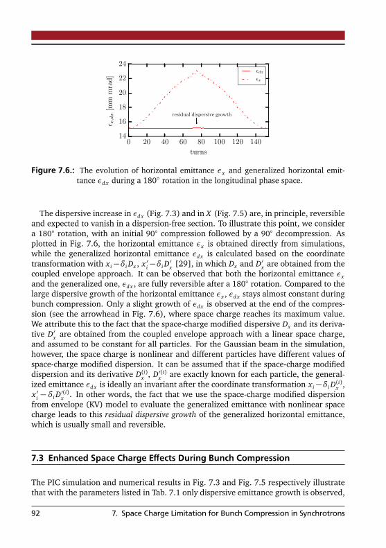
0 20 40 60 80 100 120 140
turns
14
16
18
20
22
24
ǫ x,dx[m
mmrad]
residual dispersive growth
ǫdx
ǫx
Figure 7.6.: The evolution of horizontal emittance εx and generalized horizontal emit-tance εd x during a 180 rotation in the longitudinal phase space.
The dispersive increase in εd x (Fig. 7.3) and in X (Fig. 7.5) are, in principle, reversibleand expected to vanish in a dispersion-free section. To illustrate this point, we considera 180 rotation, with an initial 90 compression followed by a 90 decompression. Asplotted in Fig. 7.6, the horizontal emittance εx is obtained directly from simulations,while the generalized horizontal emittance εd x is calculated based on the coordinatetransformation with x i−δi Dx , x ′i −δi D
′x [29], in which Dx and D′x are obtained from the
coupled envelope approach. It can be observed that both the horizontal emittance εx
and the generalized one, εd x , are fully reversible after a 180 rotation. Compared to thelarge dispersive growth of the horizontal emittance εx , εd x stays almost constant duringbunch compression. Only a slight growth of εd x is observed at the end of the compres-sion (see the arrowhead in Fig. 7.6), where space charge reaches its maximum value.We attribute this to the fact that the space-charge modified dispersive Dx and its deriva-tive D′x are obtained from the coupled envelope approach with a linear space charge,and assumed to be constant for all particles. For the Gaussian beam in the simulation,however, the space charge is nonlinear and different particles have different values ofspace-charge modified dispersion. It can be assumed that if the space-charge modifieddispersion and its derivative D(i)x , D′(i)x are exactly known for each particle, the general-ized emittance εd x is ideally an invariant after the coordinate transformation x i−δi D
(i)x ,
x ′i − δi D′(i)x . In other words, the fact that we use the space-charge modified dispersion
from envelope (KV) model to evaluate the generalized emittance with nonlinear spacecharge leads to this residual dispersive growth of the generalized horizontal emittance,which is usually small and reversible.
7.3 Enhanced Space Charge Effects During Bunch Compression
The PIC simulation and numerical results in Fig. 7.3 and Fig. 7.5 respectively illustratethat with the parameters listed in Tab. 7.1 only dispersive emittance growth is observed,
92 7. Space Charge Limitation for Bunch Compression in Synchrotrons
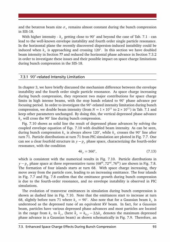
and the betatron beam size σx remains almost constant during the bunch compressionin SIS-18.
With higher intensity - ky getting close to 90 and beyond the case of Tab. 7.1 - canlead to the well-known envelope instability and fourth order single particle resonance.In the horizontal plane the recently discovered dispersion-induced instability could beinduced when kx is approaching and crossing 120. In this section we have doubledbeam intensity in Section ?? and reduced the horizontal phase advance in Section 7.3.2in order to investigate these issues and their possible impact on space charge limitationsduring bunch compression in the SIS-18.
7.3.1 90-related Intensity Limitation
In chapter 3, we have briefly discussed the mechanism difference between the envelopeinstability and the fourth order single particle resonance. As space charge increasingduring bunch compression, they represent two major contributions for space chargelimits in high intense beams, with the stop bands related to 90 phase advance perfocusing period. In order to investigate the 90-related intensity limitation during bunchcompression, we double beam intensity (from N = 1× 10¹¹ to 2× 10¹¹) in Tab. 7.1 andkeep other parameters unchanged. By doing this, the vertical depressed phase advanceky will cross the 90 line during bunch compression.
Fig. 7.10 shows as solid line the result of depressed phase advances by solving thecoupled envelope equation of Eqs. 7.10 with doubled beam intensity. As can be seen,during bunch compression kx is always above 120, while ky crosses the 90 line afterturn 71. Particle distributions at turn 71 from PIC simulation are plotted in Fig. 7.7. Onecan see a clear fourfold structure in y − py phase space, characterizing the fourth-orderresonance, with the condition
4ky = 360, (7.13)
which is consistent with the numerical results in Fig. 7.10. Particle distributions iny − py phase space at three representative turns (68th, 72nd, 76th) are shown in Fig. 7.8.The formation of four islands starts at turn 68. With space charge increasing, theymove away from the particle core, leading to an increasing emittance. The four islandsin Fig. 7.7 and Fig. 7.8 confirm that the emittance growth during bunch compressionis due to the fourth-order resonance, and no envelope instability is observed in PICsimulations.
The evolution of transverse emittances in simulation during bunch compression isshown as dashed line in Fig. 7.10. Note that the emittances start to increase at turn68, slightly before turn 71 where ky = 90. Also note that for a Gaussian beam ky isunderstood as the depressed tune of an equivalent KV beam. In fact, for a Gaussianbeam, particles have various depressed phase advances and most particles are locatedin the range from ky to ky , (here ky = k0,y − 2∆ky denotes the maximum depressedphase advance in a Gaussian beam) as shown schematically in Fig. 7.9. Therefore, an
7.3. Enhanced Space Charge Effects During Bunch Compression 93

Figure 7.7.: Particle distribution in (a) x-x ′ phase space; (b) y-y ′ phase space; (c) x-y real space and (d) longitudinal z-δ phase space at turn 72 during bunchcompression, with doubled beam intensity.
Figure 7.8.: The evolution of particle distribution in the y − y ′ phase space at final stageof bunch compression with double beam intensity at 68th, 72nd, 76th turnsduring bunch compression.
94 7. Space Charge Limitation for Bunch Compression in Synchrotrons
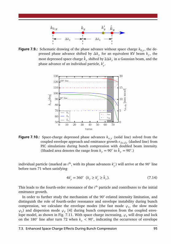
Figure 7.9.: Schematic drawing of the phase advance without space charge k0,y , the de-pressed phase advance shifted by ∆ky for an equivalent KV beam ky , themost depressed space charge ky shifted by 2∆ky in a Gaussian beam, and thephase advance of an individual particle, ki
y .
0 10 20 30 40 50 60 70
turns
50
60
70
80
90
100
110
120
130
kx,y[deg]
120 line
90 line
kx
ky
ky0
5
10
15
20
ǫ dx,dy[m
mmrad]
ǫdx
ǫdy
Figure 7.10.: Space-charge depressed phase advances kx ,y (solid line) solved from thecoupled envelope approach and emittance growth εd x ,d y (dashed line) fromPIC simulations during bunch compression with doubled beam intensity.(Shaded area denotes the range from ky = 90 to ky = 90.)
individual particle (marked as ith, with its phase advances kiy) will arrive at the 90 line
before turn 71 when satisfying
4kiy = 360 (ky ≥ ki
y ≥ ky). (7.14)
This leads to the fourth-order resonance of the ith particle and contributes to the initialemittance growth.
In order to further study the mechanism of the 90-related intensity limitation, anddistinguish the role of fourth-order resonance and envelope instability during bunchcompression, we calculate the envelope modes (the fast mode ϕ1, the slow modeϕ2) and dispersion mode ϕd [4] during bunch compression from the coupled enve-lope model, as shown in Fig. 7.11. With space charge increasing, ϕ2 will drop and lockon the 180 line after turn 72 when ky < 90, indicating the occurrence of envelope
7.3. Enhanced Space Charge Effects During Bunch Compression 95
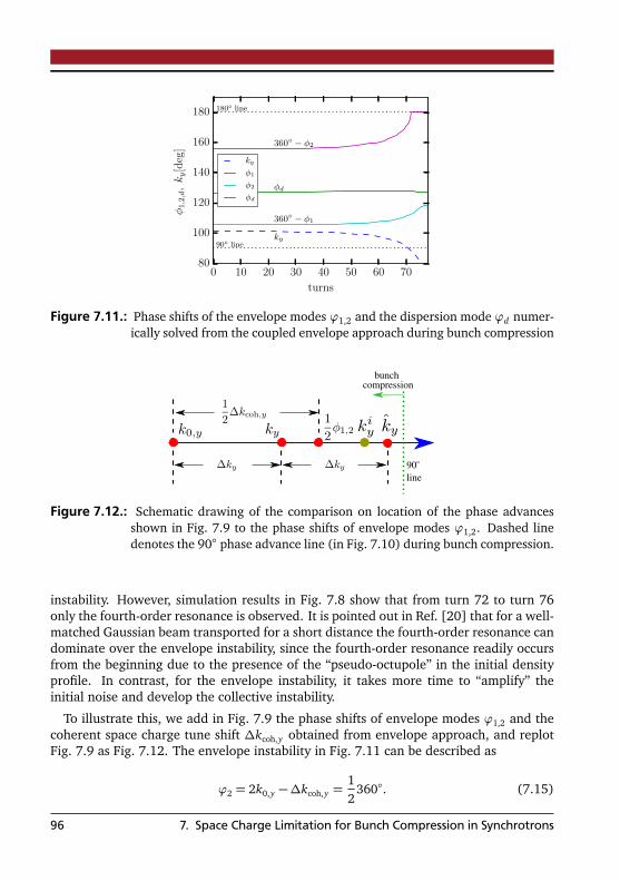
0 10 20 30 40 50 60 70
turns
80
100
120
140
160
180
φ1,2,d,ky[deg]
180 line
90 line
360 − φ2
φd
360 − φ1
ky
ky
φ1
φ2
φd
Figure 7.11.: Phase shifts of the envelope modes ϕ1,2 and the dispersion mode ϕd numer-ically solved from the coupled envelope approach during bunch compression
bunchcompression
90
line
Figure 7.12.: Schematic drawing of the comparison on location of the phase advancesshown in Fig. 7.9 to the phase shifts of envelope modes ϕ1,2. Dashed linedenotes the 90 phase advance line (in Fig. 7.10) during bunch compression.
instability. However, simulation results in Fig. 7.8 show that from turn 72 to turn 76only the fourth-order resonance is observed. It is pointed out in Ref. [20] that for a well-matched Gaussian beam transported for a short distance the fourth-order resonance candominate over the envelope instability, since the fourth-order resonance readily occursfrom the beginning due to the presence of the “pseudo-octupole” in the initial densityprofile. In contrast, for the envelope instability, it takes more time to “amplify” theinitial noise and develop the collective instability.
To illustrate this, we add in Fig. 7.9 the phase shifts of envelope modes ϕ1,2 and thecoherent space charge tune shift ∆kcoh,y obtained from envelope approach, and replotFig. 7.9 as Fig. 7.12. The envelope instability in Fig. 7.11 can be described as
ϕ2 = 2k0,y −∆kcoh,y =12
360. (7.15)
96 7. Space Charge Limitation for Bunch Compression in Synchrotrons
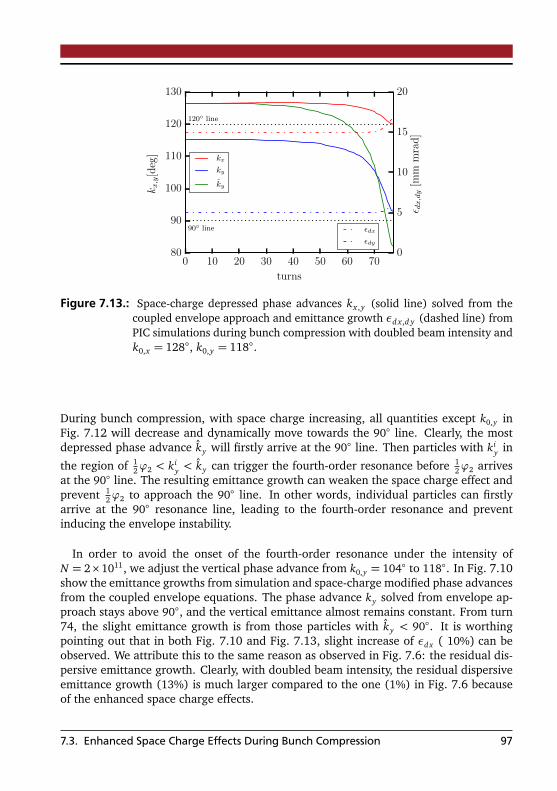
0 10 20 30 40 50 60 70
turns
80
90
100
110
120
130
kx,y[deg]
120 line
90 line
kx
ky
ky
0
5
10
15
20
ǫ dx,dy[m
mmrad]
ǫdx
ǫdy
Figure 7.13.: Space-charge depressed phase advances kx ,y (solid line) solved from thecoupled envelope approach and emittance growth εd x ,d y (dashed line) fromPIC simulations during bunch compression with doubled beam intensity andk0,x = 128, k0,y = 118.
During bunch compression, with space charge increasing, all quantities except k0,y inFig. 7.12 will decrease and dynamically move towards the 90 line. Clearly, the mostdepressed phase advance ky will firstly arrive at the 90 line. Then particles with ki
y in
the region of 12ϕ2 < ki
y < ky can trigger the fourth-order resonance before 12ϕ2 arrives
at the 90 line. The resulting emittance growth can weaken the space charge effect andprevent 1
2ϕ2 to approach the 90 line. In other words, individual particles can firstlyarrive at the 90 resonance line, leading to the fourth-order resonance and preventinducing the envelope instability.
In order to avoid the onset of the fourth-order resonance under the intensity ofN = 2×10¹¹, we adjust the vertical phase advance from k0,y = 104 to 118. In Fig. 7.10show the emittance growths from simulation and space-charge modified phase advancesfrom the coupled envelope equations. The phase advance ky solved from envelope ap-proach stays above 90, and the vertical emittance almost remains constant. From turn74, the slight emittance growth is from those particles with ky < 90. It is worthingpointing out that in both Fig. 7.10 and Fig. 7.13, slight increase of εd x ( 10%) can beobserved. We attribute this to the same reason as observed in Fig. 7.6: the residual dis-persive emittance growth. Clearly, with doubled beam intensity, the residual dispersiveemittance growth (13%) is much larger compared to the one (1%) in Fig. 7.6 becauseof the enhanced space charge effects.
7.3. Enhanced Space Charge Effects During Bunch Compression 97

Figure 7.14.: Particle distribution in (a) x-x ′ phase space; (b) y-y ′ phase space; (c) x-yreal space and (d) longitudinal z-δ phase space at 70th turn during bunchcompression, with k0,x = 122, k0,y = 104.
7.3.2 120-related Intensity Limitation
During bunch compression space charge as well as dispersion are increasing. Withsufficiently high beam intensity and designed horizontal phase advance k0,x larger than120, as is the case for SIS-18, the combined effects of space charge and dispersioncould induce the 120 dispersion instability, which is another limitation factor for bunchcompression. In order to investigate this, we adjust k0,x from 128 to 122 in Tab. 7.1and keep other parameters unchanged. By doing this, the horizontal phase advance kx
will cross the 120 line during bunch compression.Particle distributions at turn 70 from PIC simulation are plotted in Fig. 7.14, which is
similar to the case in Fig. 7.3, and no evident emittance growth has occurred up to thispoint. Fig. 7.15 shows the result of depressed phase advances by solving the coupledenvelope equation of Eqs.11 with k0,x = 122, k0,y = 104. As can be seen, during bunchcompression ky is always above 90 while kx crosses the 120 line after 70th turn.
Particle distributions in x − px phase space at three representative turns (72nd, 74th,and 76th) are shown in Fig. 7.16, from which one can see the emittance deformationand the effect of emittance growth.
The evolution of transverse emittance in simulation during bunch compression isshown as dashed line in Fig. 7.15. Note that sharp increasing of the emittance occurs
98 7. Space Charge Limitation for Bunch Compression in Synchrotrons

0 10 20 30 40 50 60 70
turns
90
95
100
105
110
115
120
125
kx,y[deg]
120 line 71thturnline
kx
ky
0
5
10
15
20
25
30
ǫ dx,dy[m
mmrad]
ǫdx
ǫdy
Figure 7.15.: Space-charge depressed phase advances kx ,y (solid line) obtained from thecoupled envelope approach and emittance growth εd x ,d y (dashed line) fromPIC simulations during bunch compression with k0,x = 122 and k0,y =104.
starting from turn 72. This is different from the case when crossing the 90 resonanceline in Fig. 7.10, in which emittance growth occurs much earlier than ky = 90. Weattribute this difference to the reason that the emittance growth in Fig. 7.14 is from the120 dispersion instability, which is a collective effect with,
ϕ1 +ϕd = 360, (7.16)
when
k0,x > 120 and kx < 120. (7.17)
The emittance growth observed in Fig. 7.15 must be distinguished from the residualdispersive growth of εd x appeared in Fig. 7.6, Fig. 7.10 and Fig. ??. The point is that,with the same beam intensity, the horizontal emittance growth (100%) in Fig. 7.15 ismuch larger than that in Fig. 7.6 (1%), Fig. 7.6 (13%) and Fig. 7.10 (13%), and can beexplained only by the dispersion-induced instability. Moreover, the dispersive emittancegrowth is characterized by an extension of emittance along the slope of the ellipse ofthe emittance in the x− x ′ plane, as shown in Fig. 7.3 and Fig. 7.14. In comparison, theevolution of particle distribution in Fig. 7.16 has no such regular extension and behaveslike the emittance growth during the envelope instability (for example, see the figuresin [17] and Fig.2 in [20]).
In order to further study the mechanism of 120-related intensity limitation, wecalculate the fast mode ϕ1, slow mode ϕ2 and dispersion mode ϕd with k0,x = 122,k0,y = 104. As shown in Fig. 7.17, with space charge increasing during bunch compres-sion, the curve ϕd will be confluent with 360−ϕ1, indicating the dispersion-instability,which is in good agreement with the sharp emittance growth at turn 71 in Fig. 7.15.
7.3. Enhanced Space Charge Effects During Bunch Compression 99

Figure 7.16.: The evolution of particle distribution in the x− x ′ phase space at final stageof bunch compression with k0,x = 122, k0,y = 104 at 72th, 74th, 76th turnsduring bunch compression.
0 10 20 30 40 50 60 70
turns
100
120
140
160
180
φ1,2,d,kx[deg] 360 − φ2
φd
360 − φ1 kx
φ1
φ2
φd
kx
Figure 7.17.: Phase shifts of the envelope modes ϕ1, ϕ2 and dispersion mode ϕd numeri-cally solved from the coupled envelope approach during bunch compressionwith k0,x = 122 and k0,y = 104. (Shaded area denotes the stop band ofthe dispersion-induced instability.)
100 7. Space Charge Limitation for Bunch Compression in Synchrotrons
The onset of the dispersion-induced instability is not inhibited compared with that ofthe envelope instability. Firstly, compared with the competition between fourth-orderresonance and envelope instability related to 90, there is no obvious single particleresonance, which exists earlier and can weaken the space charge and prevent the 120
dispersion instability. This is different from the case of the 90 envelope instability,which is suppressed by the competition with the fourth-order resonance. Secondly,the beam intensity threshold of 120 dispersion instability is much lower than that of90 envelope instability, as can be seen in the Fig.2 in Ref. [4]. Therefore, the formerinstability would need less time to develop than the latter.
7.3. Enhanced Space Charge Effects During Bunch Compression 101
102 7. Space Charge Limitation for Bunch Compression in Synchrotrons
8 Conclusions and Outlook
8.1 Conclusions
The present work in this thesis focus on a detailed study of intense beam motion andtransverse instabilities in synchrotrons, in which the role of dispersion is fully taken intobeam coherent motion. By a generalized envelope equations including space-chargemodified dispersion function, important properties of dispersion under the influence ofspace charge are discussed. Moreover, a rms-matched particle distribution with disper-sion and space charge is introduced and employed in simulation in this work.
Full numerical solutions of the generalized envelope equations and the oscillationmodel shows that a coherent dispersion mode exists, besides the well-know slow andfast envelope modes. For phase advances larger than 120 and lattice parameters similarto modern high-intensity synchrotrons, we find that the dispersion mode is unstable andinduce a novel beam instability - dispersion-induced instability. Our analysis reveals thatthis new instability in periodic focusing lattices is characterized by the confluence of thefast mode or slow envelope mode (i.e. the second order even mode) with the dispersionmode. PIC simulations using pyORBIT are performed to support the theory of dispersionmode and the dispersion-induced instability and shows good agreement.
Another important study in this thesis is that complete set of second order instanti-ates. The linearized second order moment equations derived from Chernin’s equationsoffer a unified framework to study the stability properties of all possible second ordermodes, even and odd ones, in constant or periodic focusing quadrupole lattices with-out bending. Results are compared with earlier results on mode frequencies obtainedfrom the linearized Vlasov-Poisson equation. Excellent agreement is found in the case ofthe tilting instability of odd (skew) modes in anisotropic beams and constant focusing,which confirms the equivalence of both models - on the level of second order pertur-bations. Comparing moment spectra from the perturbation equations with PIC spectrafor KV and waterbag beams, peaks pertaining to odd modes are retrieved at similarlocations. Hence this suggests that these modes also exist for more realistic beam distri-butions, like waterbag. In periodic focusing structures the stop bands of the parametriccoupled even mode sum instability and the skew mode sum instability are obtained andfound in very good agreement with PIC simulations, which completes the picture ofsecond order coherent modes in 2d high intensity beams.
As an application, we apply the theory above to study the bunch compression in circu-lar accelerators, where both dispersion and space charge play important roles. Takingthe SIS-18 in GSI as an example, the beam dynamics during bunch compression hasbeen investigated. In order to study the beam current limitation during bunch com-
103

pression, several possible beam instabilities related to phase advance of 90 and 120
during bunch compression are discussed. Detailed simulation reveals the mechanismof the beam instability during bunch compression and give the method to avoid beaminstabilities.
8.2 Outlook
We expect that the coherent dispersion mode and its instability will have implicationsfor the choice of the working point in high intensity circular accelerators. An impor-tant application would be the experimental identification of the space charge modifieddispersion mode from the transverse beam spectra: The observation of the dispersionmode could be a method to dynamically characterize the space-charge-modified dis-persion. Measurements in circular accelerators could take advantage of quadrupolarpickup signals to identify the envelope modes [79, 80] and the new coherent dispersionmode, which would give a full dynamical characterization of the relevant optical func-tions modified by space charge. Furthermore, the identified 120 stop band could beavoided during bunch compression [45, 81, 47] in synchrotrons and might play a rolein ERLs and recirculators.
The rms-matched distribution and the generalized envelope equation set includingdispersion and the corresponding envelope oscillation equitations could be employedas two complementary methods to investigate beam dynamics with space charge anddispersion.
The dispersion mode introduced here could trigger further studies of confluence withother modes [1, 73, 24]. Furthermore, the role of synchrotron motion on this new in-stability in bunched beams deserves additional study. Future studies also might have toinclude the effects of external skew magnets as well as of synchrotron motion. Correla-tions with the recently discovered instabilities induced by the dispersion mode in bentlattices also warrant further work.
104 8. Conclusions and Outlook
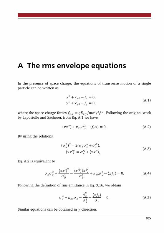
A The rms envelope equations
In the presence of space charge, the equations of transverse motion of a singleparticle can be written as
x ′′ +κx0 − fx = 0,
y ′′ +κy0 − f y = 0,(A.1)
where the space charge forces fx ,y = qEx ,y/mc2γ3β2. Following the original workby Lapostolle and Sacherer, from Eq. A.1 we have
⟨x x ′′⟩+κx0σ2x − ⟨ fx x⟩= 0. (A.2)
By using the relations
(σ2x)′′ = 2(σxσ
′′x +σ
′2x ),
⟨x x ′⟩′ = σ′2x + ⟨x x ′′⟩,(A.3)
Eq. A.2 is equivalent to
σxσ′′x +⟨x x ′⟩2
σ2x
−⟨x ′2⟩⟨x2⟩σ2
x
+ κx0σ2x − ⟨x fx⟩= 0. (A.4)
Following the definition of rms emittance in Eq. 3.16, we obtain
σ′′x +κx0σx −ε2
x
σ3x
−⟨x fx⟩σx
= 0. (A.5)
Similar equations can be obtained in y-direction.
105

An important contribution by Sacherer is that the term ⟨x fx⟩ in the above equa-tion is independent of the type of particle distributions and has the same value asfor the distributions, which has the same rms transverse beam size, i.e.,
⟨x fx⟩=Ksc
2σx
σx +σy, (A.6)
⟨x fx⟩+ ⟨y f y⟩=Ksc
2. (A.7)
With above relations, the rms envelope equations take the form
σ′′x + κx0(s)σx −Ksc
2(σx +σy)−ε2
x
σ3x
= 0,
σ′′y + κy0(s)σy −Ksc
2(σx +σy)−ε2
y
σ3y
= 0.
(A.8)
106 A. The rms envelope equations

B The envelope modes of mismatchoscillation
In the framework of Ref. [17], the two modes can be obtained via firstly solv-ing numerically Eqs. 3.19, from which the matched solution used as coefficientsin Eqs. 3.26, and secondly fundamental modes can be found via the method ofsolution matrix. In the following, we will adopt another method to solve the per-turbation system in Eqs. 3.26.
For brevity, the coupled system in Eqs. 3.26 can be rewritten as
ξ′′ + a1ξ+ a2ζ= 0,
ζ′′ + a3ζ+ a2ξ= 0,(B.1)
with the coefficients
a1 = κx0 +Ksc
2(σx0 +σy0)2+
3ε2x
σ4x0
,
a2 =Ksc
2(σx0 +σy0)2,
a3 = κy0 +Ksc
2(σx0 +σy0)2+
3ε2y
σ4y0
.
(B.2)
We assume a set of variables (p1, p2) to represent the envelope oscillation in thedecoupled form,
p′′1 + k1p1 = 0,
p′′2 + k2p2 = 0,(B.3)
through a coordinate rotation on the variables (ξ,ζ),
p1p2
=
cosϑ sinϑ− sinϑ cosϑ
ξζ
. (B.4)
107
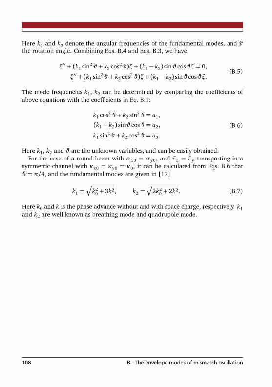
Here k1 and k2 denote the angular frequencies of the fundamental modes, and ϑthe rotation angle. Combining Eqs. B.4 and Eqs. B.3, we have
ξ′′ + (k1 sin2 ϑ+ k2 cos2 ϑ)ζ+ (k1 − k2) sinϑ cosϑζ= 0,
ζ′′ + (k1 sin2 ϑ+ k2 cos2 ϑ)ζ+ (k1 − k2) sinϑ cosϑξ.(B.5)
The mode frequencies k1, k2 can be determined by comparing the coefficients ofabove equations with the coefficients in Eq. B.1:
k1 cos2 ϑ+ k2 sin2 ϑ = a1,
(k1 − k2) sinϑ cosϑ = a2,
k1 sin2 ϑ+ k2 cos2 ϑ = a3.
(B.6)
Here k1, k2 and ϑ are the unknown variables, and can be easily obtained.For the case of a round beam with σx0 = σy0, and εx = εy transporting in a
symmetric channel with κx0 = κy0 = κ0, it can be calculated from Eqs. B.6 thatϑ = π/4, and the fundamental modes are given in [17]
k1 =q
k20 + 3k2, k2 =
q
2k20 + 2k2. (B.7)
Here k0 and k is the phase advance without and with space charge, respectively. k1and k2 are well-known as breathing mode and quadrupole mode.
108 B. The envelope modes of mismatch oscillation

C The movements of eigenvaluesFig. C.1 illustrates the movements of the four eigenvalues of the perturbation mapof Eq. 3.29, for the case of a round beam travelling in an alternating gradientchannel with the phase advance k0,x = k0,y = 60. The two arrows in the upperhalf complex plane denotes the two envelopes, with their conjugate counterpartexisting in the lower half plane. In the absence of space charge (ηx = 1.0), the twoeigenvalues lie on unit circle and are overlapped. and no envelope instability occur.As beam current increasing, the phase shifts of the two modes start to move and areseperated (see the subplot with ηx = 0.1). As the beam current keeps increasing,the phase shifts of the slow mode are equal to the one of fast mode, indicating theoccurrence of the envelope instability (see the subplot with ηx = 0.22). For strongspace charge (ηx = 0.34), the two modes separates from each other again.
109

−1.5−1.0−0.5 0.0 0.5 1.0 1.5−1.5
−1.0
−0.5
0.0
0.5
1.0
1.5
Im(λ)
ηx = 1.0
−1.5−1.0−0.5 0.0 0.5 1.0 1.5−1.5
−1.0
−0.5
0.0
0.5
1.0
1.5ηx = 0.9
−1.5−1.0−0.5 0.0 0.5 1.0 1.5
Re(λ)
−1.5
−1.0
−0.5
0.0
0.5
1.0
1.5
Im(λ)
ηx = 0.78
−1.5−1.0−0.5 0.0 0.5 1.0 1.5
Re(λ)
−1.5
−1.0
−0.5
0.0
0.5
1.0
1.5ηx = 0.66
Figure C.1.: Movement of the eigenvalues λ with increasing beam intensity for k0 = 60
case in four representative cases: ηx = 0.0, 0.1, 0.22, 0.34.
110 C. The movements of eigenvalues
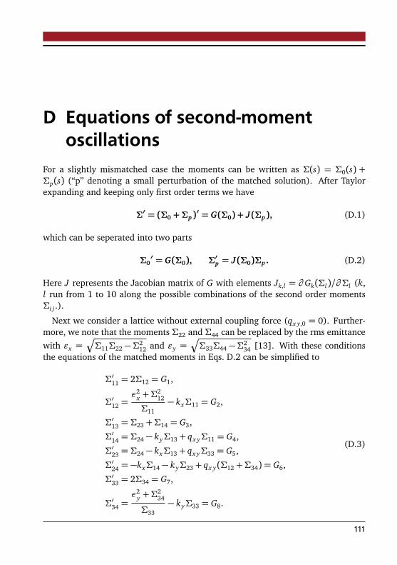
D Equations of second-momentoscillations
For a slightly mismatched case the moments can be written as Σ(s) = Σ0(s) +Σp(s) (“p” denoting a small perturbation of the matched solution). After Taylorexpanding and keeping only first order terms we have
Σ′ = (Σ0 +Σp)′ = G(Σ0) + J(Σp), (D.1)
which can be seperated into two parts
Σ0′ = G(Σ0), Σ′p = J(Σ0)Σp . (D.2)
Here J represents the Jacobian matrix of G with elements Jk,l = ∂ Gk(Σl)/∂Σl (k,l run from 1 to 10 along the possible combinations of the second order momentsΣi j .).
Next we consider a lattice without external coupling force (qx y,0 = 0). Further-more, we note that the moments Σ22 and Σ44 can be replaced by the rms emittance
with εx =q
Σ11Σ22 −Σ212 and εy =
q
Σ33Σ44 −Σ234 [13]. With these conditions
the equations of the matched moments in Eqs. D.2 can be simplified to
Σ′11 = 2Σ12 = G1,
Σ′12 =ε2
x +Σ212
Σ11− kxΣ11 = G2,
Σ′13 = Σ23 +Σ14 = G3,
Σ′14 = Σ24 − kyΣ13 + qx yΣ11 = G4,
Σ′23 = Σ24 − kxΣ13 + qx yΣ33 = G5,
Σ′24 = −kxΣ14 − kyΣ23 + qx y(Σ12 +Σ34) = G6,
Σ′33 = 2Σ34 = G7,
Σ′34 =ε2
y +Σ234
Σ33− kyΣ33 = G8.
(D.3)
111
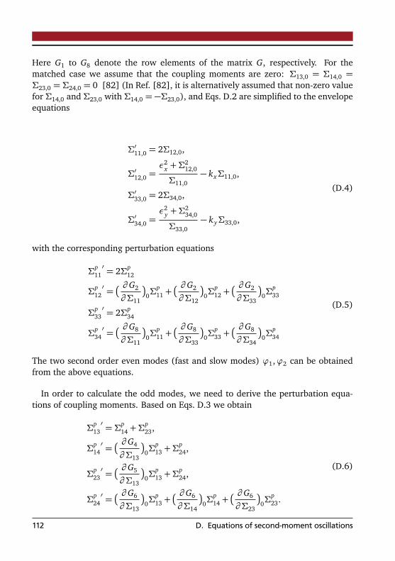
Here G1 to G8 denote the row elements of the matrix G, respectively. For thematched case we assume that the coupling moments are zero: Σ13,0 = Σ14,0 =Σ23,0 = Σ24,0 = 0 [82] (In Ref. [82], it is alternatively assumed that non-zero valuefor Σ14,0 and Σ23,0 with Σ14,0 = −Σ23,0), and Eqs. D.2 are simplified to the envelopeequations
Σ′11,0 = 2Σ12,0,
Σ′12,0 =ε2
x +Σ212,0
Σ11,0− kxΣ11,0,
Σ′33,0 = 2Σ34,0,
Σ′34,0 =ε2
y +Σ234,0
Σ33,0− kyΣ33,0,
(D.4)
with the corresponding perturbation equations
Σp11′ = 2Σp
12
Σp12′ =
∂ G2
∂Σ11
0Σp11 +
∂ G2
∂Σ12
0Σp12 +
∂ G2
∂Σ33
0Σp33
Σp33′ = 2Σp
34
Σp34′ =
∂ G8
∂Σ11
0Σp11 +
∂ G8
∂Σ33
0Σp33 +
∂ G8
∂Σ34
0Σp34
(D.5)
The two second order even modes (fast and slow modes) ϕ1,ϕ2 can be obtainedfrom the above equations.
In order to calculate the odd modes, we need to derive the perturbation equa-tions of coupling moments. Based on Eqs. D.3 we obtain
Σp13′ = Σp
14 +Σp23,
Σp14′ =
∂ G4
∂Σ13
0Σp13 +Σ
p24,
Σp23′ =
∂ G5
∂Σ13
0Σp13 +Σ
p24,
Σp24′ =
∂ G6
∂Σ13
0Σp13 +
∂ G6
∂Σ14
0Σp14 +
∂ G6
∂Σ23
0Σp23.
(D.6)
112 D. Equations of second-moment oscillations

Note that in the matched case, Σ13,0 = Σ14,0 = Σ23,0 = Σ24,0 = 0, and from Eqs. 5.3and Eqs. 5.4 we have
∂∆qx y
∂Σ11
0 =∂∆qx y
∂Σ33
0 = 0,
∂∆qx y
∂Σ13=
K2
1S0(Sx + Sy)
.(D.7)
The Eqs. D.7 mean that the space charge coupling term has no influence on thematched solution, but on the perturbation second order odd modes. With thematched beam moments from Eqs. D.4, the perturbations in Eqs. D.5 and Eqs. D.6can be used to calculate the two even as well as the two odd modes.
113

E Partial derivatives of the Jacobianmatrix
In the absence of the external skew focusing strength, the partial derivatives ofthe Jacobian with respect to second moments takes a simplified form, listed in thefollowing tables.
∂ G1 ∂ G2 ∂ G3 ∂ G4
∂Σ11 0 −ε2
x+Σ212
Σ211− kx +Σ11
∂ qx x∂Σ11
0 Σ13∂ qy y∂Σ11
∂Σ12 2 2Σ12Σ11
0 0∂Σ13 0 0 0 −ky
∂Σ14 0 0 1 0∂Σ23 0 0 1 0∂Σ24 0 0 0 1
∂Σ33 0 Σ11∂ qx xΣ33
0 Σ13∂ qy y∂Σ33
∂Σ34 0 0 0 0
∂ G5 ∂ G6 ∂ G7 ∂ G8
∂Σ11 Σ13∂ qx x∂Σ11
Σ14∂ qx x∂Σ11
+Σ23∂ qy y∂Σ11
0 Σ33∂ qy y∂Σ11
∂Σ12 0 0 0 0∂Σ13 −kx 0 0 0∂Σ14 0 −kx 0 0∂Σ23 0 −ky 0 0∂Σ24 1 0 0 0
∂Σ33 Σ13∂ qx x∂Σ33
Σ14∂ qx x∂Σ33
+Σ23∂ qy y∂Σ33
0 −ε2
y+Σ234
Σ233− ky +Σ33
∂ qy y∂Σ33
∂Σ34 0 0 2 2Σ34Σ33
114
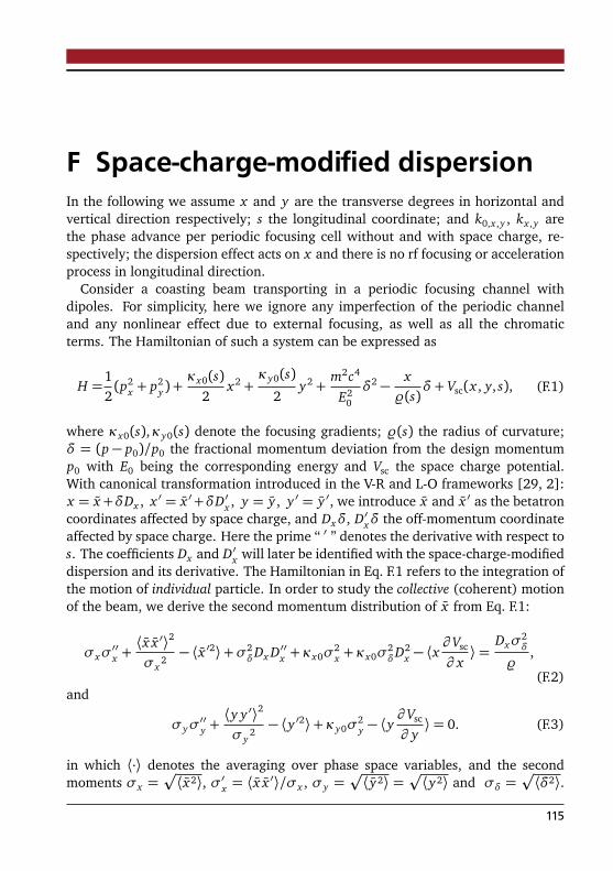
F Space-charge-modified dispersionIn the following we assume x and y are the transverse degrees in horizontal andvertical direction respectively; s the longitudinal coordinate; and k0,x ,y , kx ,y arethe phase advance per periodic focusing cell without and with space charge, re-spectively; the dispersion effect acts on x and there is no rf focusing or accelerationprocess in longitudinal direction.
Consider a coasting beam transporting in a periodic focusing channel withdipoles. For simplicity, here we ignore any imperfection of the periodic channeland any nonlinear effect due to external focusing, as well as all the chromaticterms. The Hamiltonian of such a system can be expressed as
H =12(p2
x + p2y) +
κx0(s)2
x2 +κy0(s)
2y2 +
m2c4
E20
δ2 −x%(s)
δ+ Vsc(x , y, s), (F.1)
where κx0(s),κy0(s) denote the focusing gradients; %(s) the radius of curvature;δ = (p− p0)/p0 the fractional momentum deviation from the design momentump0 with E0 being the corresponding energy and Vsc the space charge potential.With canonical transformation introduced in the V-R and L-O frameworks [29, 2]:x = x+δDx , x ′ = x ′+δD′x , y = y , y ′ = y ′, we introduce x and x ′ as the betatroncoordinates affected by space charge, and Dxδ, D′xδ the off-momentum coordinateaffected by space charge. Here the prime “ ′ ” denotes the derivative with respect tos. The coefficients Dx and D′x will later be identified with the space-charge-modifieddispersion and its derivative. The Hamiltonian in Eq. F.1 refers to the integration ofthe motion of individual particle. In order to study the collective (coherent) motionof the beam, we derive the second momentum distribution of x from Eq. F.1:
σxσ′′x +⟨ x x ′⟩2
σx2− ⟨ x ′2⟩+σ2
δDx D′′x + κx0σ2x + κx0σ
2δD2
x − ⟨x∂ Vsc
∂ x⟩=
Dxσ2δ
%,
(F.2)and
σyσ′′y +⟨y y ′⟩2
σy2− ⟨y ′2⟩+κy0σ
2y − ⟨y
∂ Vsc
∂ y⟩= 0. (F.3)
in which ⟨·⟩ denotes the averaging over phase space variables, and the secondmoments σx =
p
⟨ x2⟩, σ′x = ⟨ x x ′⟩/σx , σy =p
⟨ y2⟩ =p
⟨y2⟩ and σδ =p
⟨δ2⟩.
115

Following Sacherer’s approach [13], i.e., ⟨x ∂ Vsc∂ x ⟩ is independent of the form of
particle distribution, we have:
⟨x∂ Vsc
∂ x⟩=
Kscσ2x
2X (X + Y )+
Kscσ2δ
D2x
2X (X + Y )(F.4)
with,
⟨x∂ Vsc
∂ x⟩= ⟨ x
∂ Vsc
∂ x⟩+ Dx⟨δ
∂ Vsc
∂ x⟩, (F.5)
which is correct in good approximation if the dispersive term of Eq. F.4 is not domi-nant. Here X 2 = σ2
x +σ2δ
D2x and Y = σy . Ksc is the space charge perveance defined
by Ksc = 2NL rc/(β2γ3), with NL the number of particles per length, rc the classicalproton radius, β and γ the relativistic factors. Eq. F.4 indicates that in the presenceof dispersion, the beam coherent motion characterized by the second moments canbe expressed as a linear superposition of two aspects: the betatron motion and thedispersion motion, independent of the form of particle distribution.
The space-charge-modified dispersion function can be defined in the combinationof Eq. F.1 to Eq. F.5:
d2Dx
ds2+
κx0(s)−Ksc
2X (X + Y )
Dx =1%(s)
, (F.6)
with the corresponding rms envelope equations in the presence of both dispersionand space charge:
d2σx
ds2+
κx0(s)−Ksc
2X (X + Y )
σx −ε2
d x
σ3x
= 0, (F.7a)
d2σy
ds2+
κy0(s)−Ksc
2Y (X + Y )
σy −ε2
d y
σ3y
= 0, (F.7b)
where εd x =Æ
⟨ x2⟩⟨ x ′2⟩ − ⟨ x x ′⟩2 (similar in εd y), is the generalized rms emittanceintroduced in V-R and L-O theory, and can be defined by
ε2x = ε
2d x(
X 2
σ2x
) +σ2δ(σx D′x −σ
′x Dx)
2, (F.8)
116 F. Space-charge-modified dispersion

and εy = εd y . Here εx and εy are the rms transverse emittances usually used:εx =
Æ
⟨x2⟩⟨p2x⟩ − ⟨x px⟩2 (similar for εy), which are not invariant in the presence
of dispersion.
117

G The movements of eigenvalueswith dispersion
In the presence of dispersion, the movement of eigenvalues of perturbation map inEq. 6.20 for k0 = 120 case are discussed as follows with four representative cases:ηx = 0.1, 0.25, 0.35, 0.6. As shown in Fig. G.1, three arrows in the upper halfcomplex plane denotes the three modes, with their conjugate counterpart existingin the lower half plane. For weak space charge with ηx = 0.1, all three eigen valueslie on unit circle and no envelope instability occur. For ηx = 0.25, the fast modeis locked on the real axis (ϕ1 = 180), indicating parametric instability take place.With beam current go on increasing, the phase shifts of the slow mode are equal tothe one of fast mode and the confluent resonance take places (ϕ1 = ϕ2). For strongspace charge (ηx = 0.6), the two modes separates from each other again. Note thatin the case of k0 = 120 the instabilities are triggered by either the unstable fastmode or the slow mode, and the dispersion mode keeps stable.
The movement of eigenvalues in k0 = 130 case are discussed as follows withsix representative cases (see Fig. G.2): ηx = 0.05, 0.1, 0.15, 0.25, 0.3, 0.35.Beam starts with being stable under weak space charge (ηx = 0.05). With beamcurrent increasing, the phase shift of dispersion mode will “catch up with” theone of slow mode and overlap with each other, indicating the occurrence of 120
dispersion instability (shown in the cases of ηx = 0.1 and ηx = 0.15). When beamcurrent keeps on increasing, the slow mode becomes larger and gets separatedfrom the dispersion mode (ηx = 0.25), until the fast mode reaches the 180 line(ηx = 0.3) which indicates that the occurrence of the usual 90 envelope instabilitytriggered by parametric resonance takes place. Under stronger space charge effect(ηx = 0.35), the slow mode will overlap with the fast mode, indicating occurrenceof the confluence resonance.
118

−1.5−1.0−0.5 0.0 0.5 1.0 1.5−1.5
−1.0
−0.5
0.0
0.5
1.0
1.5
Im(λ)
ηx = 0.1
−1.5−1.0−0.5 0.0 0.5 1.0 1.5−1.5
−1.0
−0.5
0.0
0.5
1.0
1.5ηx = 0.25
−1.5−1.0−0.5 0.0 0.5 1.0 1.5
Re(λ)
−1.5
−1.0
−0.5
0.0
0.5
1.0
1.5
Im(λ)
ηx = 0.35
−1.5−1.0−0.5 0.0 0.5 1.0 1.5
Re(λ)
−1.5
−1.0
−0.5
0.0
0.5
1.0
1.5ηx = 0.6
Figure G.1.: Movement of eigen value λ with increasing beam intensity for k0 = 120
case with dispersion in four representative cases: ηx = 0.1, 0.25, 0.35, 0.6.
119
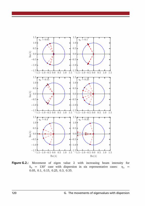
−1.5−1.0−0.5 0.0 0.5 1.0 1.5−1.5
−1.0
−0.5
0.0
0.5
1.0
1.5
Im(λ)
ηx = 0.05
−1.5−1.0−0.5 0.0 0.5 1.0 1.5−1.5
−1.0
−0.5
0.0
0.5
1.0
1.5ηx = 0.1
−1.5−1.0−0.5 0.0 0.5 1.0 1.5−1.5
−1.0
−0.5
0.0
0.5
1.0
1.5
Im(λ)
ηx = 0.15
−1.5−1.0−0.5 0.0 0.5 1.0 1.5−1.5
−1.0
−0.5
0.0
0.5
1.0
1.5ηx = 0.25
−1.5−1.0−0.5 0.0 0.5 1.0 1.5
Re(λ)
−1.5
−1.0
−0.5
0.0
0.5
1.0
1.5
Im(λ)
ηx = 0.3
−1.5−1.0−0.5 0.0 0.5 1.0 1.5
Re(λ)
−1.5
−1.0
−0.5
0.0
0.5
1.0
1.5ηx = 0.35
Figure G.2.: Movement of eigen value λ with increasing beam intensity fork0 = 130 case with dispersion in six representative cases: ηx =0.05, 0.1, 0.15, 0.25, 0.3, 0.35.
120 G. The movements of eigenvalues with dispersion

H Lists
Acronyms
AGD Alternative gradient focusing system withdispersion
CERN Organisation européenne pour la recherchenucléaire
CFD Constant gradient focusing system with dis-persion
ERL Energy recovery linacFAIR Facility for Antiproton and Ion Research in
Europe GmbHFFT fast Fourier transformationGSI GSI Helmholtzzentrum für Schwerionen-
forschung GmbHPIC Particle In CellQD Defocusing quadrupoleQF Focusing quadrupolerf radio frequencyRMS root mean squareSC Space chargeSIS100 Schwerionensynchrotron 100 (heavy ion
synchrotron)SIS18 Schwerionensynchrotron 18 (heavy ion
synchrotron)
Symbols
Term Unit DescriptionKsc 1 transverse space charge perveancem kg Rest mass
121
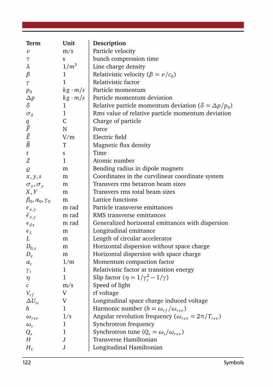
Term Unit Descriptionv m/s Particle velocityτ s bunch compression timeλ 1/m3 Line charge densityβ 1 Relativistic velocity (β = v/c0)γ 1 Relativistic factorp0 kg ·m/s Particle momentum∆p kg ·m/s Particle momentum deviationδ 1 Relative particle momentum deviation (δ =∆p/p0)σδ 1 Rms value of relative particle momentum deviationq C Charge of particle~F N Force~E V/m Electric field~B T Magnetic flux densityt s TimeZ 1 Atomic number% m Bending radius in dipole magnetsx , y, s m Coordinates in the curvilinear coordinate systemσx ,σy m Transvers rms betatron beam sizesX , Y m Transvers rms total beam sizesβ0,α0,γ0 m Lattice functionsεx ,y m rad Particle transverse emittancesεx ,y m rad RMS transverse emittancesεd x m rad Generalized horizontal emittances with dispersionεL m Longitudinal emittanceL m Length of circular acceleratorD0,x m Horizontal dispersion without space chargeDx m Horizontal dispersion with space chargeαc 1/m Momentum compaction factorγt 1 Relativistic factor at transition energyη 1 Slip factor (η= 1/γ2
t − 1/γ)c m/s Speed of lightVr f V rf voltage∆Usc V Longitudinal space charge induced voltageh 1 Harmonic number (h=ωr f /ωrev )ωrev 1/s Angular revolution frequency (ωrev = 2π/Trev )ωs 1 Synchrotron frequencyQs 1 Synchrotron tune (Qs =ωs/ωrev )H J Transverse HamiltonianHL J Longitudinal Hamiltonian
122 Symbols
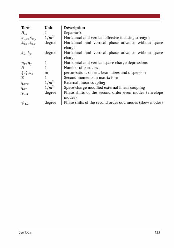
Term Unit DescriptionHsx J Separatrixκ0,x ,κ0,y 1/m2 Horizontal and vertical effective focusing strengthk0,x , k0,y degree Horizontal and vertical phase advance without space
chargekx , ky degree Horizontal and vertical phase advance without space
chargeηx ,ηy 1 Horizontal and vertical space charge depressionsN 1 Number of particlesξ,ζ, dx m perturbations on rms beam sizes and dispersionΣ 1 Second moments in matrix formqx y0 1/m2 External linear couplingqx y 1/m2 Space-charge modified external linear couplingϕ1,2 degree Phase shifts of the second order even modes (envelope
modes)ψ1,2 degree Phase shifts of the second order odd modes (skew modes)
Symbols 123

List of Figures
1.1. Schematic drawing of a drift-tube linac (DTL). Particles feel electric fieldat each gaps between two adjacent tubes to increase kinetic energy, andfeel zero field when traveling inside the tubes. . . . . . . . . . . . . . . . . . 3
1.2. Schematic drawing of a synchrotron. When particles travel along the ringthrough each element: dipoles guide the trajectory of particles alongthe ring; quadrupoles provide transverse focusing force; injection andextraction magnets (septum magnets) are used to beam injection andbeam extraction; RF cavities provide the electric field for acceleration. . . 3
1.3. Layout of the FAIR project. Ion beams generated at ion source (at thestart point of UNILAC) are accelerated via UNILAC to 11.4 MeV/u, andinjected to booster synchrotron SIS-18, where the typical kinetic energyof particles are at the range of 200 MeV/u to 4 GeV/u. Those particles aretransported to SIS-100 for further acceleration, where the final kineticenergy of particles can reach up to 28 GeV/u (for protons). Particles canbe extracted from SIS-100 for various experiments.(figure from [3]) . . . 4
1.4. Bunch compression by fast bunch rotation. The bunch in the horizontalposition is rotated by 90 into an upright position. . . . . . . . . . . . . . . . 6
2.1. Curvilinear coordinate system for particle motion in circular accelerators. 102.2. Single particle emittance in z-direction: the invariant of a particle beta-
tron motion in (z, z′) phase space. The elliptical area enclosed is equalto πεz . The maximum amplitude of betatron motion is
Æ
β0,zεz and themaximum divergence angle is
p
γ0,zεz . . . . . . . . . . . . . . . . . . . . . . . 142.3. Schematic drawing of particle trajectories with different momenta in
bending magnets. Due to different moment pi , the magnetic rigidityB%i = pi/q(i = 1, 2,3) of each particle is different, defining differenttrajectories. . . . . . . . . . . . . . . . . . . . . . . . . . . . . . . . . . . . . . . . 16
2.4. Dispersion functions (in green color) and beta functions (βx in black andβy in red) calculated from MAD-X [53] in one periodic structure in SIS-18. 18
2.5. The separatrix with ϕs = 0, 30, 60. The separatrix area decreases withϕs increases. . . . . . . . . . . . . . . . . . . . . . . . . . . . . . . . . . . . . . . . 20
2.6. Schematic drawing of the distribution of electromagnetic fields in thebeam cylinder model. The upper plot (a) shows the electromagneticfields on the profile of the beam cylinder; and the lower plot (b) showsthe electromagnetic fields in the cross section of the beam cylinder. . . . . 22
124

2.7. Comparison between the particle distribution (upper plot) and the linecharge density (lower plot) of a coasting beam and a bunched beam. . . . 24
2.8. Schematic drawing of the synchrotron motion of particles with variousamplitudes in the longitudinal phase space and the corresponding space-charge tune shifts. . . . . . . . . . . . . . . . . . . . . . . . . . . . . . . . . . . . 25
2.9. Schematic drawing of electromagnetic field distribution for a coastingbeam with a beam pipe. EW and Es are caused by impedance. The reddashed rectangular loop is the path integral of Faraday’s law. . . . . . . . . 26
3.1. Schematic drawing of the cross section of a K-V beam, on which particlesdistribute random-uniformly on the ellipse with the semi-major axis Xand the major semi-axis Y . . . . . . . . . . . . . . . . . . . . . . . . . . . . . . . 31
3.2. The emittance εx and the rms emittance εx of a K-V distribution. . . . . . . 343.3. An example of numerical solutions of Eqs. 3.19. The rms envelopes of
the matched beam and a mismatched beam in five alternating gradientfocusing periods. . . . . . . . . . . . . . . . . . . . . . . . . . . . . . . . . . . . . 36
3.4. Schematic drawing of the oscillations of the two eigenmodes. . . . . . . . . 393.5. Round beam case,k0,x = k0,y = k0 = 60: Phase shifts ϕ1,2 of the funda-
mental mismatch oscillation versus tune depression in x . . . . . . . . . . . 393.6. Mechanical analogy of mismatch oscillation and instability. . . . . . . . . . 403.7. k0 = 120 case. Upper: Phase shifts ϕ1 and ϕ2 versus tune depression;
Lower: Growth factor |λ| versus tune depression. (The region betweenthe dashed line denotes the stop band of the envelope instability. . . . . . 41
3.8. The evolution of the beam rms envelope with mached, envelope mis-match oscillation, and envelope instability. . . . . . . . . . . . . . . . . . . . . 42
3.9. Schematic drawing of the parabolic distribution, on which particles dis-tribute random-uniformly on the ellipse with the semi-major axis lm andthe semi-minor axis xm. . . . . . . . . . . . . . . . . . . . . . . . . . . . . . . . . 43
4.1. Structure of the envelope solver code. . . . . . . . . . . . . . . . . . . . . . . . 464.2. A typical cycle of PIC in a particle simulation program. The particle are
numbered as i, the grid indices are j. (Figure from Ref. [68]) . . . . . . . . 474.3. Comparison of rms beam size for three periodic cell between simulations
and envelope equation. . . . . . . . . . . . . . . . . . . . . . . . . . . . . . . . . 484.4. Comparison of the transverse space charge forces in a K-V beam calcu-
lated from pyORBIT and theoretical formula. . . . . . . . . . . . . . . . . . . 494.5. Comparison of the space-charge tune spread in a Gaussian beam calcu-
lated from pyORBIT and theoretical formula. . . . . . . . . . . . . . . . . . . 49
5.1. Round beam case, k0,x = k0,y = k0 = 60: Phase shifts ϕ1,2,ψ1 versus tunedepression in x in a constant focusing channel. . . . . . . . . . . . . . . . . . 55
5.2. Elliptical beam case, k0,x = 60, k0,y = 66.7 and εx/εy = 2: Phase shiftsof coherent even modes ϕ1,2 and odd modes ψ1,2 versus tune depressionin x in a constant focusing channel. . . . . . . . . . . . . . . . . . . . . . . . . 55
List of Figures 125

5.3. Elliptical beam case, k0,x = 60, k0,y = 66.7: Beam spectrum of ⟨x y⟩from PIC simulation of KV distribution (red solid) and waterbag (WB)distribution (blue solid), compared with the analytical results (dottedblack lines) of phase shifts of second order odd sum and difference modesψ1,2, for different values of ηx in a constant focusing channel. . . . . . . . 56
5.4. Growth rate of difference odd mode (normalized) for constant ky/k0,y =0.8 and εx/εy = 2 as a function of the betatron tune ratio, indicating thetilting instability in a constant focusing channel. . . . . . . . . . . . . . . . . 57
5.5. Perturbation theory results for both types of sum envelope instabilitiesin a periodic focusing system. Upper plot (a): Phase shifts of ϕ1,2, ψ1,2
verses tune depression in x; Lower plot (b): Corresponding growth fac-tors per lattice period (continuous lines), and comparison with final emit-tance growth factors (dashed lines, normalized to initial values) for PICsimulation of same cases. . . . . . . . . . . . . . . . . . . . . . . . . . . . . . . . 58
5.6. Real space distributions for three consecutive cells at early stage of cou-pled even mode sum instability with initial ηx = 0.6. . . . . . . . . . . . . . 59
5.7. Real space distribution for three representative consecutive cells at earlystage of skew mode sum instability with initial ηx = 0.67. . . . . . . . . . . 60
5.8. Phase shifts of ϕ1,2,ψ1,2 verses tune depression in x with fixed k0,y = 145
and varying k0,x = 40 (yellow), 50 (red), 60 (blue) and 70 (green). . . 605.9. Tune diagram as scan of growth factor λ obtained from perturbation matrix. 615.10.Enlarged scans of the two opposite corner zones in Fig. 5.9. . . . . . . . . . 61
6.1. An example of the space-charge depression ηx ,y as the functions of rmsmomentum spread σδ for a fixed beam intensity. . . . . . . . . . . . . . . . . 65
6.2. Left plot: tune depression in y (solid line) and betatron beam size ratioσx0/σy0 (dashed line) versus beam current (in the unit of ηx ). Rightplot: total beam size ratio X0/Y0 (solid line) and dispersion ratio (dashedline) versus beam current (in the unit of ηx ). . . . . . . . . . . . . . . . . . . 68
6.3. Space-charge-modified betatron functions in x (left plot) and y (rightplot) with (solid line) and without (dashed line) dispersion effect in oneAGD periodic cell, for ηx = 0.0,0.1, 0.2. . . . . . . . . . . . . . . . . . . . . . . 71
6.4. Space-charge-modified dispersion functions in one AGD periodic cell(solid line) with varying beam current (ηx = 0.0, 0.1,0.2.), comparedwith the dispersion in CFD case (dotted line) and the approximated dis-persion evaluated from the scaling law (dashed line). . . . . . . . . . . . . . 71
6.5. An example of the SCD distribution (red) in x−x ′ phase space (a) and x−y real space (b), generated from a KV distribution (blue) by coordinatetransformation. εd x = 10.0 mm mrad, σδ = 1.0× 10⁻³. . . . . . . . . . . . . 72
6.6. The orthogonal decomposition of total rms beam size as a 2-D vector formatched and mismatched cases. . . . . . . . . . . . . . . . . . . . . . . . . . . 73
6.7. k0 = 60 case: Phase shifts ϕ1,ϕ2 and ϕ3 versus tune depression ηx with(solid line) and without (dashed line) dispersion. . . . . . . . . . . . . . . . 75
126 List of Figures
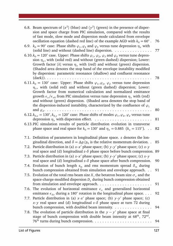
6.8. Beam spectrum of ⟨x2⟩ (blue) and ⟨y2⟩ (green) in the presence of disper-sion and space charge from PIC simulation, compared with the resultsof fast mode, slow mode and dispersion mode calculated from envelopeoscillation equation (dashed red line) of the example AGD with k0 = 60 . 76
6.9. k0 = 90 case: Phase shifts ϕ1,ϕ2 and ϕ3 versus tune depression ηx with(solid line) and without (dashed line) dispersion. . . . . . . . . . . . . . . . 77
6.10.k0 = 120 case. Upper: Phase shifts ϕ1, ϕ2, ϕ3 and ϕd versus tune depres-sion ηx , with (solid red) and without (green dashed) dispersion; Lower:Growth factor |λ| versus ηx with (red) and without (green) dispersion.(Shaded area denotes the stop band of the envelope instability modifiedby dispersion: parametric resonance (shallow) and confluent resonance(dark)). . . . . . . . . . . . . . . . . . . . . . . . . . . . . . . . . . . . . . . . . . . 78
6.11.k0 = 130 case: Upper: Phase shifts ϕ1,ϕ2, ϕd versus tune depressionηx , with (solid red) and without (green dashed) dispersion; Lower:Growth factor from numerical calculation and normalized emittancegrowth εx/εx0 from PIC simulation versus tune depression ηx with (red)and without (green) dispersion. (Shaded area denotes the stop band ofthe dispersion-induced instability, characterized by the confluence of ϕ1
and ϕd . . . . . . . . . . . . . . . . . . . . . . . . . . . . . . . . . . . . . . . . . . . 806.12.k0,x = 130, k0,y = 120 case: Phase shifts of modes ϕ1,ϕ2, ϕd versus tune
depression ηx with dispersion effect. . . . . . . . . . . . . . . . . . . . . . . . 816.13.PIC simulation results of particle distribution evolution in transverse
phase space and real space for k0 = 130 and ηx = 0.885 (kx = 115). . . 82
7.1. Definition of parameters in longitudinal phase space. z denotes the lon-gitudinal direction, and δ =∆p/p0 is the relative momentum deviation. . 85
7.2. Particle distribution in (a) x-x ′ phase space; (b) y-y ′ phase space; (c) x-yreal space and (d) longitudinal z-δ phase space before bunch compression. 89
7.3. Particle distribution in (a) x-x ′ phase space; (b) y-y ′ phase space; (c) x-yreal space and (d) longitudinal z-δ phase space after bunch compression. 90
7.4. Evolution of bunch length zm and rms momentum spread δm duringbunch compression obtained from simulation and envelope approach. . . 91
7.5. Evolution of the total rms beam size X , the betatron beam size σx and thespace-charge-modified dispersion Dx during bunch compression obtainedfrom simulation and envelope approach. . . . . . . . . . . . . . . . . . . . . . 91
7.6. The evolution of horizontal emittance εx and generalized horizontalemittance εd x during a 180 rotation in the longitudinal phase space. . . . 92
7.7. Particle distribution in (a) x-x ′ phase space; (b) y-y ′ phase space; (c)x-y real space and (d) longitudinal z-δ phase space at turn 72 duringbunch compression, with doubled beam intensity. . . . . . . . . . . . . . . . 94
7.8. The evolution of particle distribution in the y − y ′ phase space at finalstage of bunch compression with double beam intensity at 68th, 72nd,76th turns during bunch compression. . . . . . . . . . . . . . . . . . . . . . . . 94
List of Figures 127

7.9. Schematic drawing of the phase advance without space charge k0,y , thedepressed phase advance shifted by ∆ky for an equivalent KV beam ky ,the most depressed space charge ky shifted by 2∆ky in a Gaussian beam,and the phase advance of an individual particle, ki
y . . . . . . . . . . . . . . . 957.10.Space-charge depressed phase advances kx ,y (solid line) solved from the
coupled envelope approach and emittance growth εd x ,d y (dashed line)from PIC simulations during bunch compression with doubled beam in-tensity. (Shaded area denotes the range from ky = 90 to ky = 90.) . . . . 95
7.11.Phase shifts of the envelope modes ϕ1,2 and the dispersion mode ϕd
numerically solved from the coupled envelope approach during bunchcompression . . . . . . . . . . . . . . . . . . . . . . . . . . . . . . . . . . . . . . . 96
7.12.Schematic drawing of the comparison on location of the phase advancesshown in Fig. 7.9 to the phase shifts of envelope modes ϕ1,2. Dashed linedenotes the 90 phase advance line (in Fig. 7.10) during bunch compres-sion. . . . . . . . . . . . . . . . . . . . . . . . . . . . . . . . . . . . . . . . . . . . . 96
7.13.Space-charge depressed phase advances kx ,y (solid line) solved from thecoupled envelope approach and emittance growth εd x ,d y (dashed line)from PIC simulations during bunch compression with doubled beam in-tensity and k0,x = 128, k0,y = 118. . . . . . . . . . . . . . . . . . . . . . . . . 97
7.14.Particle distribution in (a) x-x ′ phase space; (b) y-y ′ phase space; (c)x-y real space and (d) longitudinal z-δ phase space at 70th turn duringbunch compression, with k0,x = 122, k0,y = 104. . . . . . . . . . . . . . . . . 98
7.15.Space-charge depressed phase advances kx ,y (solid line) obtained fromthe coupled envelope approach and emittance growth εd x ,d y (dashedline) from PIC simulations during bunch compression with k0,x = 122
and k0,y = 104. . . . . . . . . . . . . . . . . . . . . . . . . . . . . . . . . . . . . . 997.16.The evolution of particle distribution in the x − x ′ phase space at final
stage of bunch compression with k0,x = 122, k0,y = 104 at 72th, 74th,76th turns during bunch compression. . . . . . . . . . . . . . . . . . . . . . . . 100
7.17.Phase shifts of the envelope modes ϕ1, ϕ2 and dispersion mode ϕd nu-merically solved from the coupled envelope approach during bunch com-pression with k0,x = 122 and k0,y = 104. (Shaded area denotes the stopband of the dispersion-induced instability.) . . . . . . . . . . . . . . . . . . . 100
C.1. Movement of the eigenvalues λ with increasing beam intensity for k0 =60 case in four representative cases: ηx = 0.0, 0.1, 0.22, 0.34. . . . . . . . 110
G.1. Movement of eigen value λ with increasing beam intensity for k0 = 120
case with dispersion in four representative cases: ηx = 0.1, 0.25, 0.35, 0.6.119G.2. Movement of eigen value λ with increasing beam intensity for k0 = 130
case with dispersion in six representative cases: ηx = 0.05, 0.1, 0.15, 0.25, 0.3, 0.35.120
128 List of Figures

List of Tables
6.1. Main parameters of the example CFD . . . . . . . . . . . . . . . . . . . . . . . 686.2. Main parameters of the example AGD . . . . . . . . . . . . . . . . . . . . . . . 70
7.1. Main parameters for an example bunch compression in SIS-18 . . . . . . . 88
129

Bibliography[1] Ingo Hofmann. Stability of anisotropic beams with space charge. Physical
Review E, 57(4), 1998. 1, 5, 51, 54, 56, 104
[2] S.Y. Lee and H. Okamoto. Space-charge dominated beams in synchrotrons.Physical review letters, 80(23):5133, 1998. 1, 5, 64, 115
[3] www.fair-center.eu. 1, 4, 124
[4] Y.S. Yuan, O. Boine-Frankenheim, G. Franchetti, and I. Hofmann. Dispersion-induced beam instability in circular accelerators. Physical Review Letters,118(15):154801, 2017. 1, 57, 59, 63, 72, 73, 76, 95, 101
[5] D. Chernin. Evolution of rms beam envelopes in transport systems with linearxy coupling. Part. Accel., 24:29–44, 1988. 2, 51, 52
[6] Yao-Shuo Yuan, Oliver Boine-Frankenheim, and Ingo Hofmann. Modeling ofsecond order space charge driven coherent sum and difference instabilities.Physical Review Accelerators and Beams, 20(10):104201, 2017. 2
[7] Ernest D. Courant, M. Stanley Livingston, and Hartland S. Snyder. Thestrong-focusing synchroton - a new high energy accelerator. Physical Review,88(5):1190, 1952. 2, 35
[8] Edwin M. McMillan. The synchrotron - a proposed high energy particle accel-erator. Physical Review, 68(5-6):143, 1945. 2, 18
[9] Vladimir Isaakovich Veksler. A new method of acceleration of relativistic par-ticles. J. Phys., 9:153–158, 1945. 2, 18
[10] www.gsi.de. 4
[11] I.M. Kapchinskij and V.V. Vladimirskij. Limitations of proton beam current ina strong focusing linear accelerator associated with the beam space charge.In Proceedings of the International Conference on High Energy Accelerators andInstrumentation, page 274, 1959. 5, 29
[12] Pierre M. Lapostolle. Possible emittance increase through filamentation dueto space charge in continuous beams. IEEE Transactions on Nuclear Science,18(3):1101–1104, 1971. 5, 29, 33
130

[13] Frank J. Sacherer. Rms envelope equations with space charge. IEEE Transac-tions on Nuclear Science, 18(3):1105–1107, 1971. 5, 29, 33, 111, 116
[14] Robert L. Gluckstern. Analytic model for halo formation in high current ionlinacs. Physical review letters, 73(9):1247, 1994. 5
[15] T.P. Wangler, K.R. Crandall, R. Ryne, and T.S. Wang. Particle-core model fortransverse dynamics of beam halo. Physical review special topics-acceleratorsand beams, 1(8):084201, 1998. 5
[16] Chiping Chen and Ronald C Davidson. Nonlinear resonances and chaoticbehavior in a periodically focused intense charged-particle beam. Physicalreview letters, 72(14):2195, 1994. 5
[17] J. Struckmeier, M. Reiser, and J. Klabunde. On the stability and emittancegrowth of different particle phase-space distributions in a long magneticquadrupole channel. Part. Accel., 15:47–65, 1984. 5, 38, 41, 57, 75, 99,107, 108
[18] Steven M. Lund and Boris Bukh. Stability properties of the transverse enve-lope equations describing intense ion beam transport. Physical Review SpecialTopics-Accelerators and Beams, 7(2):024801, 2004. 5
[19] Chao Li and Ya Liang Zhao. Envelope instability and the fourth order reso-nance. Physical Review Special Topics-Accelerators and Beams, 17(12):124202,2014. 5
[20] Ingo Hofmann and Oliver Boine-Frankenheim. Space-charge structural in-stabilities and resonances in high-intensity beams. Physical review letters,115(20):204802, 2015. 5, 59, 96, 99
[21] Hung-Chun Chao and S.Y. Lee. Simulations of beam envelope dynamics incircular accelerators. Physical Review Special Topics-Accelerators and Beams,18(2):024202, 2015. 5
[22] Oliver Boine-Frankenheim, Ingo Hofmann, and Jürgen Struckmeier. Paramet-ric sum envelope instability of periodically focused intense beams. Physics ofPlasmas, 23(9):090705, 2016. 5, 51, 57, 81
[23] Robert L. Gluckstern. Oscillation modes in two dimensional beams. Technicalreport, Univ. of Massachusetts, Amherst), 1970. 5
Bibliography 131

[24] I. Hofmann, G. Franchetti, O. Boine-Frankenheim, J. Qiang, and R.D. Ryne.Space charge resonances in two and three dimensional anisotropic beams.Physical Review Special Topics-Accelerators and Beams, 6(2):024202, 2003. 5,57, 104
[25] Dong-O Jeon, Kyung Ryun Hwang, Ji-Ho Jang, Hyunchang Jin, and HyojaeJang. Sixth-order resonance of high-intensity linear accelerators. Physicalreview letters, 114(18):184802, 2015. 5
[26] D. Jeon, L. Groening, and G. Franchetti. Fourth order resonance of a highintensity linear accelerator. Physical Review Special Topics-Accelerators andBeams, 12(5):054204, 2009. 5, 41
[27] L. Groening, W. Barth, W. Bayer, G. Clemente, L. Dahl, P. Forck, P. Gerhard,I. Hofmann, M.S. Kaiser, M. Maier, et al. Experimental evidence of the 90stop band in the gsi unilac. Physical review letters, 102(23):234801, 2009. 5
[28] L. Groening, I. Hofmann, W. Barth, W. Bayer, G. Clemente, L. Dahl, P. Forck,P. Gerhard, M.S. Kaiser, M. Maier, et al. Experimental evidence of space chargedriven emittance coupling in high intensity linear accelerators. Physical reviewletters, 103(22):224801, 2009. 5
[29] Marco Venturini and Martin Reiser. Rms envelope equations in the presenceof space charge and dispersion. Physical review letters, 81(1):96, 1998. 5, 64,87, 92, 115
[30] Marco Venturini and Martin Reiser. Self-consistent beam distributions withspace charge and dispersion in a circular ring lattice. Physical Review E,57(4):4725, 1998. 5
[31] S. Bernal, B. Beaudoin, T. Koeth, and P.G. O’Shea. Smooth approximationmodel of dispersion with strong space charge for continuous beams. PhysicalReview Special Topics-Accelerators and Beams, 14(10):104202, 2011. 5
[32] Masanori Ikegami, Shinji Machida, and Tomonori Uesugi. Particle-core anal-ysis of dispersion effects on beam halo formation. Physical Review SpecialTopics-Accelerators and Beams, 2(12):124201, 1999. 5
[33] J.A. Holmes, V.V. Danilov, J.D. Galambos, D. Jeon, and D.K. Olsen. Spacecharge dynamics in high intensity rings. Physical Review Special Topics-Accelerators and Beams, 2(11):114202, 1999. 5, 70
132 Bibliography

[34] S. Cousineau, S.Y. Lee, J.A. Holmes, V. Danilov, and A. Fedotov. Space chargeinduced resonance excitation in high intensity rings. Physical Review SpecialTopics-Accelerators and Beams, 6(3):034205, 2003. 5, 70
[35] Oleksandr Chorniy, Oliver Boine-Frankenheim, Peter Hülsmann, and Peter J.Spiller. Fast compression of intense heavy-ion bunches in sis18. Proc. of HBworkshop, 2010. 6, 88
[36] P. Hülsmann, R. Balss, U. Laier, and H. Klingbeil. Bunch compression for fair.In Proceedings of the PAC, volume 9, 2009. 6
[37] Oliver Boine-Frankenheim. The fair accelerators: highlights and challenges.Proc. IPAC2010, Kyoto, Japan, page 2430, 2010. 6
[38] K. Blasche, O. Boine-Frankenheim, H. Eickhoff, M. Emmerling, B. Franczak,I. Hofmann, K. Kaspar, U. Ratzinger, and P. Spiller. Bunch compression in theheavy ion synchrotron sis at gsi. In Europ. Part. Acc. Conf., Stockholm, Sweden,pages 1347–1349, 1998. 6
[39] S.M. Lund, O. Boine-Frankenheim, G. Franchetti, I. Hofmann, and P. Spiller.Simulations of axial bunch compression in heavy ion rings for plasma physicsapplications at gsi. In Particle Accelerator Conference, 1999. Proceedings of the1999, volume 3, pages 1785–1787. IEEE, 1999. 6
[40] P. Spiller, J. Ahrens, K. Blasche, M. Emmerling, O. Boine-Frankenheim,B. Franczak, P. Hulsmann, G. Moritz, C. Muhle, W. Vinzenz, et al. A newhigh-intensity synchrotron sis100 with strong bunch compression for gsi. InParticle Accelerator Conference, 2001. PAC 2001. Proceedings of the 2001, vol-ume 5, pages 3278–3280. IEEE, 2001. 6
[41] K.Y. Ng. Space-charge effects on bunch rotation in the longitudinal phasespace. In Particle Accelerator Conference, 2001. PAC 2001. Proceedings of the2001, volume 4, pages 2893–2895. IEEE, 2001. 6
[42] Takashi Kikuchi, Mitsuo Nakajima, Kazuhiko Horioka, and Takeshi Katayama.Beam instability induced by space charge oscillation during final beam bunch-ing for heavy ion inertial fusion. Physical Review Special Topics-Acceleratorsand Beams, 7(3):034201, 2004. 6
[43] T. Kikuchi, S.M. Lund, T. Katayama, and S. Kawata. Bunch compression ina ring for future riken projects. Nuclear Instruments and Methods in PhysicsResearch Section A: Accelerators, Spectrometers, Detectors and Associated Equip-ment, 544(1-2):393–397, 2005. 6
Bibliography 133
[44] T. Kikuchi and K. Horioka. Beam behavior under a non-stationary state inhigh-current heavy ion beams. Nuclear Instruments and Methods in PhysicsResearch Section A: Accelerators, Spectrometers, Detectors and Associated Equip-ment, 606(1-2):31–36, 2009. 6
[45] G. Franchetti, I. Hofmann, and G. Rumolo. Effect of space charge on bunchcompression near the transition. Physical Review Special Topics-Acceleratorsand Beams, 3(8):084201, 2000. 6, 83, 84, 104
[46] K.Y. Ng. Space-charge effects on beam rotation at the compressor ring. Techni-cal report, Fermi National Accelerator Laboratory (FNAL), Batavia, IL, 2013.6, 83
[47] Ye Zou, Jingyu Tang, Jingfang Chen, Xiao Li, and Hong Sun. Short-bunchextraction in a rapid cycling synchrotron. Physical Review Special Topics-Accelerators and Beams, 17(6):060101, 2014. 6, 104
[48] J. Clerk Maxwell. A dynamical theory of the electromagnetic field. Philosoph-ical transactions of the Royal Society of London, 155:459–512, 1865. 9
[49] John David Jackson. Classical electrodynamics. John Wiley & Sons, 2007. 10
[50] S.Y. Lee. Accelerator physics. World Scientific Publishing Co Inc, 2004. 11, 12,15, 69, 86
[51] George William Hill. On the part of the motion of the lunar perigee whichis a function of the mean motions of the sun and moon. Acta mathematica,8(1):1–36, 1886. 11
[52] Gaston Floquet. Sur les equations differentielles lineaires. Ann. ENS [2],12(1883):47–88, 1883. 12
[53] http://mad.web.cern.ch/mad. 18, 45, 124
[54] Martin Reiser. Theory and design of charged particle beams. John Wiley &Sons, 2008. 21, 29, 32, 33, 44, 66
[55] Alexander Wu Chao, Karl Hubert Mess, Maury Tigner, and Frank Zimmer-mann. Handbook of accelerator physics and engineering. World scientific, 2013.21
[56] Karlheinz Schindl. Space charge. (CERN-PS-99-012-DI):26 p, Mar 1999. 21
134 Bibliography
[57] J.A. MacLachlan. Longitudinal phase space tracking with space charge andwall coupling impedance. Fermi National Accelerator Laboratory, FN-446,1987. 25
[58] Ronald C. Davidson. Physics of nonneutral plasmas. Imperial College PressLondon, 2001. 29
[59] A. Vlasov. On the kinetic theory of an assembly of particles with collectiveinteraction. Russ. Phys. J., 9:25–40, 1945. 29
[60] Tao Pang. An introduction to computational physics, 1999. 36
[61] M. Reiser. Periodic focusing of intense beams. Part. Accel., 8:167–182, 1978.37
[62] S.Y. Lee and A. Riabko. Envelope hamiltonian of an intense charged-particlebeam in periodic solenoidal fields. Physical Review E, 51(2):1609, 1995. 40
[63] David Neuffer. Longitudinal motion in high current ion beams-a self-consistent phase space distribution with an envelope equation. IEEE Transac-tions on Nuclear Science, 26(3):3031–3033, 1979. 42, 43
[64] https://www.python.org. 45
[65] http://www.numpy.org. 46
[66] https://www.scipy.org. 46
[67] Roger W. Hockney and James W. Eastwood. Computer simulation using parti-cles. crc Press, 1988. 46, 48
[68] C.K. Birdsall and A.B. Langdon. Plasma physics via computer simulation. CRCpress, 2004. 46, 47, 125
[69] Ingo Hofmann and Oliver Boine-Frankenheim. Grid dependent noise andentropy growth in anisotropic 3d particle-in-cell simulation of high intensitybeams. Physical Review Special Topics-Accelerators and Beams, 17(12):124201,2014. 47
[70] Andrei Shishlo, Sarah Cousineau, Jeffrey Holmes, and Timofey Gorlov. Theparticle accelerator simulation code pyorbit. Procedia Computer Science,51:1272–1281, 2015. 47, 54, 81, 87
[71] J.D. Galambos, J.A. Holmes, D.K. Olsen, A. Luccio, and J. Beebe-Wang. Orbituser manual version 1.10. SNS/ORNL/AP Technical Note 011, Rev. 1, 1999.47
Bibliography 135

[72] Alexey Burov and Valeri Lebedev. Transverse instabilities of coasting beamswith space charge. Physical Review Special Topics-Accelerators and Beams,12(3):034201, 2009. 50
[73] G. Franchetti, I. Hofmann, and M. Aslaninejad. Collective emittance exchangewith linear space charge forces and linear coupling. Physical review letters,94(19):194801, 2005. 51, 104
[74] I. Hofmann and O. Boine-Frankenheim. Resonant emittance transfer drivenby space charge. Physical review letters, 87(3):034802, 2001. 51
[75] I. Hofmann and G. Franchetti. Self-consistent study of space-charge-drivencoupling resonances. Physical Review Special Topics-Accelerators and Beams,9(5):054202, 2006. 51, 57
[76] Ingo Hofmann and Oliver Boine-Frankenheim. Parametric instabilities in 3dperiodically focused beams with space charge. Physical Review Acceleratorsand Beams, 20(1):014202, 2017. 51, 75
[77] A. Goswami, P. Sing Babu, and V.S. Pandit. Beam dynamics and stability analy-sis of an intense beam in a continuously twisted quadrupole focusing channel.The European Physical Journal Plus, 131(11):393, 2016. 52
[78] Hong Qin, Moses Chung, and Ronald C. Davidson. Generalized kapchinskij-vladimirskij distribution and envelope equation for high-intensity beams in acoupled transverse focusing lattice. Physical review letters, 103(22):224802,2009. 52
[79] R. Bär, I. Hofmann, P. Moritz, and U. Oeftiger. Measurement of space-charge-induced frequency shifts of quadrupolar beam oscillations in the sis. NuclearInstruments and Methods in Physics Research Section A: Accelerators, Spectrom-eters, Detectors and Associated Equipment, 415(1):460–463, 1998. 104
[80] R. Singh, O. Boine-Frankenheim, O. Chorniy, P. Forck, R. Haseitl, W. Kauf-mann, P. Kowina, K. Lang, and T. Weiland. Interpretation of transverse tunespectra in a heavy-ion synchrotron at high intensities. Physical Review SpecialTopics-Accelerators and Beams, 16(3):034201, 2013. 104
[81] K.M. Fung, M. Ball, C.M. Chu, B. Hamilton, S.Y. Lee, and K.Y. Ng. Bunchlength compression manipulations. Physical Review Special Topics-Acceleratorsand Beams, 3(10):100101, 2000. 104
136 Bibliography

[82] John J. Barnard and Bojan Losic. Envelope modes of beams with angular mo-mentum. Technical report, Lawrence Livermore National Laboratory (LLNL),Livermore, CA, 2000. 112
Bibliography 137

Yao-shuo YuanCurriculum Vitae
Schlossgartenstr.8Darmstadt, 64289 Germany
H (0049) 15902668543B [email protected]
Personal- Date of Birth: March 15, 1987.- Citizenship: China- Languages: Chinese (native), English (fluent), German (basic)- Hobbies: Table tennis, Jogging
Education2014–2018 PhD candidate, Technische Universität Darmstadt, Darmstadt, Germany.
Thesis title: Space-charge driven transverse beam instabilities in synchrotrons2009–2014 Master of Science in Physics, University of Chinese Academy of Sciences, Beijing, China.
Thesis title: Development of a simulation program for proton synchrotrons and its application onCSNS/RCS.
2005–2009 Bachelor of Science in Physics, Northeast Normal University, Changchun, China.Thesis title: Study of the number of the neutron yields in a D-T neutron tube.
Key publications- Y. S. Yuan, O. Boine-Frankenheim, G. Franchetti and I. Hofmann, Dispersion-InducedBeam Instability in Circular Accelerators, Physical Review Letters, 118, 154801 (2017).
- Yao-Shuo Yuan, Oliver Boine-Frankenheim, and Ingo Hofmann, Modeling of secondorder space charge driven coherent sum and difference instabilities, Physical ReviewAccelerators and Beams 20, 104201 (2017).
- YUAN Yao-Shuo, LI Kai-Wei, WANG Na, Yoshiro Irie, WANG Sheng, Study of the beamloading effect in the CSNS/RCS, Chinese Physics C, 39, 047003 (2015).
- YUAN Yao-Shuo, WANG Na, XU Shou-Yan, YUAN Yue, WANG Sheng, Theoreticalstudy of a dual harmonic system and its application to the CSNS/RCS, Chinese PhysicsC, 39, 127002 (2015).
- Yao-Shuo Yuan, Na Wang, Shou-Yan Xu, Sheng Wang, A code for the optimizationof RF voltage waveform and longitudinal beam dynamics simulation in an RCS, NuclearInstruments and Methods in Physics Research A, 729, pp 864-869 (2013).
Computer and software skills- Programming Languages: C++, Python- Operating system: Windows, Linux- Office: MSOffice, LibreOffice, Latex