Space and Plasma Physics Department - DiVA portal562693/FULLTEXT01.pdf · Space and Plasma Physics...
82
Transcript of Space and Plasma Physics Department - DiVA portal562693/FULLTEXT01.pdf · Space and Plasma Physics...

Space and Plasma Physics DepartmentKTH, Kungliga Tekniska Hogskolan
SE-100 44 StockholmSweden
PRELIMINARY MISSION ANALYSIS ANDDESIGN FOR A SMALL SATELLITE SWARM
September 5, 2012
Author:Noravidhya Tanapura
Supervisor:Nickolay Ivchenko
Master of Science ThesisStockholm, Sweden 2012

Abstract
The thesis is a preliminary mission analysis and design of a small satellite swarm. The concept of themission is to probe altitudes between 200 km and 6000 km to study the structures and dynamics ofthe magnetic field aligned currents. The mission lifetime is about 3 months. Aerodynamic drag at lowaltitudes is used for orbit and formation control. During the perigee passage, the satellite would deceleratedue to drag, therefore, reducing its apogee. In addition, the attitude control of the spacecraft during theperigee passage could be used for formation control by changing its cross-sectional area. The simulationsindicated that an appropriate insertion orbit should be at the perigee of 168 km and an apogee of 6000km. Moreover, from the orbital decay simulations, it was found that by maintaining a constant ram-facingarea of 0.1 m2, it is possible for the satellite to decay in 90 days. The attitude simulations show that for atleast one perigee passage at a perigee altitude of 168 km, the satellite is able to maintain its attitude andnot tumble throughout the trajectory. In addition, investigation of the leader-follower satellite formationyielded that the relative translation of a circular orbit oscillates in all relative directions whereas in anelliptical orbit it only oscillates in the cross-track direction. Furthermore, the simulation has also shownthat the relative translation of a leader-follower formation with a elliptical reference orbit, would spiralout of the radial-cross-track plane.


Acknowledgements
It would not have been possible for me to complete an undertaking as challenging as this project on myown. I would like to give special thanks to my supervisor Dr. Nickolay Ivchenko, for the opportunityto work on such a project and my gratitude for his patience and guidance that nudged me in the rightdirection when I needed it.
I would like to thank my parents for their endless source of inspiration and motivation throughoutmy journey, for I could not have imagined coming this far without their support and vision.
Finally, I would like to thank all my friends here at KTH and all those who have helped me alongthe way, for your invaluable support and feedback during the course of my studies.
Noravidhya Tanapura


I know that I am mortal and ephemeral. But when I searchfor the close-knit encompassing convolutions of the stars, myfeet no longer touch the earth, but in the presence of Zeushimself I take my fill of ambrosia which the gods produce.
-Kepler’s epigram ascribed to Ptolemy


Contents
1 Introduction 21.1 Background . . . . . . . . . . . . . . . . . . . . . . . . . . . . . . . . . . . . . . . . . . . . 21.2 Problem Statement . . . . . . . . . . . . . . . . . . . . . . . . . . . . . . . . . . . . . . . . 31.3 Scope . . . . . . . . . . . . . . . . . . . . . . . . . . . . . . . . . . . . . . . . . . . . . . . 31.4 Thesis Overview . . . . . . . . . . . . . . . . . . . . . . . . . . . . . . . . . . . . . . . . . 3
2 Theoretical Background 42.1 Orbital Mechanics . . . . . . . . . . . . . . . . . . . . . . . . . . . . . . . . . . . . . . . . 4
2.1.1 The Two-Body Problem . . . . . . . . . . . . . . . . . . . . . . . . . . . . . . . . . 42.1.2 Equation of Relative Motion . . . . . . . . . . . . . . . . . . . . . . . . . . . . . . 52.1.3 Classical Orbital Elements . . . . . . . . . . . . . . . . . . . . . . . . . . . . . . . . 62.1.4 Special Perturbation: Cowell’s Method . . . . . . . . . . . . . . . . . . . . . . . . . 72.1.5 Orbit Perturbation: Aerodynamic Drag . . . . . . . . . . . . . . . . . . . . . . . . 82.1.6 Orbit Perturbation: Non-spherical Earth . . . . . . . . . . . . . . . . . . . . . . . . 8
2.2 Attitude Kinematics . . . . . . . . . . . . . . . . . . . . . . . . . . . . . . . . . . . . . . . 92.2.1 Coordinate System and Rotation Matrix . . . . . . . . . . . . . . . . . . . . . . . . 92.2.2 Direction Cosine Matrix . . . . . . . . . . . . . . . . . . . . . . . . . . . . . . . . . 102.2.3 Euler Angles . . . . . . . . . . . . . . . . . . . . . . . . . . . . . . . . . . . . . . . 102.2.4 Euler’s Principal Rotation . . . . . . . . . . . . . . . . . . . . . . . . . . . . . . . . 112.2.5 Euler Parameters (Quaternions) . . . . . . . . . . . . . . . . . . . . . . . . . . . . 122.2.6 Kinematic Differential Equations . . . . . . . . . . . . . . . . . . . . . . . . . . . . 13
2.3 Attitude Dynamics . . . . . . . . . . . . . . . . . . . . . . . . . . . . . . . . . . . . . . . . 142.3.1 Rotational Dynamics . . . . . . . . . . . . . . . . . . . . . . . . . . . . . . . . . . . 142.3.2 Gravity Gradient Torque . . . . . . . . . . . . . . . . . . . . . . . . . . . . . . . . 162.3.3 Magnetic Torque . . . . . . . . . . . . . . . . . . . . . . . . . . . . . . . . . . . . . 172.3.4 Aerodynamic Torque . . . . . . . . . . . . . . . . . . . . . . . . . . . . . . . . . . . 18
3 Orbital Decay 193.1 Comparing Atmospheric Models . . . . . . . . . . . . . . . . . . . . . . . . . . . . . . . . 19
3.1.1 Jacchia J70 Model . . . . . . . . . . . . . . . . . . . . . . . . . . . . . . . . . . . . 193.1.2 NRLMSISE-00 Model . . . . . . . . . . . . . . . . . . . . . . . . . . . . . . . . . . 253.1.3 Summary of Atmospheric Models . . . . . . . . . . . . . . . . . . . . . . . . . . . . 32
3.2 Decay Lifetime Simulation . . . . . . . . . . . . . . . . . . . . . . . . . . . . . . . . . . . . 333.2.1 Methodology . . . . . . . . . . . . . . . . . . . . . . . . . . . . . . . . . . . . . . . 333.2.2 Effect of Atmospheric Drag . . . . . . . . . . . . . . . . . . . . . . . . . . . . . . . 333.2.3 Effect of J2 Perturbation . . . . . . . . . . . . . . . . . . . . . . . . . . . . . . . . 343.2.4 Effect of different ram-facing areas . . . . . . . . . . . . . . . . . . . . . . . . . . . 363.2.5 Summary of Simulations . . . . . . . . . . . . . . . . . . . . . . . . . . . . . . . . . 36
4 Satellite Attitude Simulation 384.1 Satellite Geometry . . . . . . . . . . . . . . . . . . . . . . . . . . . . . . . . . . . . . . . . 38
4.1.1 Satellite Dimensions and Mass Properties . . . . . . . . . . . . . . . . . . . . . . . 394.1.2 Center of Gravity . . . . . . . . . . . . . . . . . . . . . . . . . . . . . . . . . . . . . 404.1.3 Principal Moments of Inertia . . . . . . . . . . . . . . . . . . . . . . . . . . . . . . 40
iv

Contents Contents
4.2 Attitude Simulation . . . . . . . . . . . . . . . . . . . . . . . . . . . . . . . . . . . . . . . 414.2.1 Attitude Propagation . . . . . . . . . . . . . . . . . . . . . . . . . . . . . . . . . . 414.2.2 Aerodynamic Torque with Partial Accomodation Coefficient . . . . . . . . . . . . . 42
4.3 Torque Profiles . . . . . . . . . . . . . . . . . . . . . . . . . . . . . . . . . . . . . . . . . . 454.3.1 Pitch Torque . . . . . . . . . . . . . . . . . . . . . . . . . . . . . . . . . . . . . . . 484.3.2 Yaw and Roll Torque Profiles . . . . . . . . . . . . . . . . . . . . . . . . . . . . . . 50
4.4 Pitch Dynamics . . . . . . . . . . . . . . . . . . . . . . . . . . . . . . . . . . . . . . . . . . 524.4.1 Initial Orbit Conditions for Pitch Dynamics . . . . . . . . . . . . . . . . . . . . . . 524.4.2 Simulation Results . . . . . . . . . . . . . . . . . . . . . . . . . . . . . . . . . . . . 52
4.5 Summary . . . . . . . . . . . . . . . . . . . . . . . . . . . . . . . . . . . . . . . . . . . . . 54
5 Passively Stabilized Perigee Passage 555.1 Initial Conditions for Perigee Passage . . . . . . . . . . . . . . . . . . . . . . . . . . . . . 555.2 Simulation Results . . . . . . . . . . . . . . . . . . . . . . . . . . . . . . . . . . . . . . . . 565.3 Summary . . . . . . . . . . . . . . . . . . . . . . . . . . . . . . . . . . . . . . . . . . . . . 57
6 Satellite Formation Design 586.1 Coordinate Frame . . . . . . . . . . . . . . . . . . . . . . . . . . . . . . . . . . . . . . . . 586.2 Formation Dynamics . . . . . . . . . . . . . . . . . . . . . . . . . . . . . . . . . . . . . . . 596.3 Satellite Formation Simulation . . . . . . . . . . . . . . . . . . . . . . . . . . . . . . . . . 616.4 Summary . . . . . . . . . . . . . . . . . . . . . . . . . . . . . . . . . . . . . . . . . . . . . 63
7 Conclusion 64
v

List of Figures
1.1 Illustration of 2-U and 3-U Cube Satellite. [1] . . . . . . . . . . . . . . . . . . . . . . . . . 2
2.1 Geometry of an Ellipse and Orbital Parameters. [2] . . . . . . . . . . . . . . . . . . . . . . 52.2 Classical Orbital Elements. [3] . . . . . . . . . . . . . . . . . . . . . . . . . . . . . . . . . 72.3 Illustration of Encke’s method. [4] . . . . . . . . . . . . . . . . . . . . . . . . . . . . . . . 72.4 Shows ECI as N, A and B reference frame. [5] . . . . . . . . . . . . . . . . . . . . . . . . . 92.5 Euler angle rotation sequence (3-2-1). [6] . . . . . . . . . . . . . . . . . . . . . . . . . . . 112.6 Illustration of Euler’s principal rotation theorem. [6] . . . . . . . . . . . . . . . . . . . . . 112.7 Time differentiation in rotating frame. [7] . . . . . . . . . . . . . . . . . . . . . . . . . . . 142.8 Gravity gradient torques on a low-Earth orbit satellite. [8] . . . . . . . . . . . . . . . . . . 17
3.1 J70: Density maps at 300 km altitude of 3 months showing high and solar activity conditions. 213.2 J70: Density map of the solar maximum-minimum ratio for different altitudes and latitudes
of different months. . . . . . . . . . . . . . . . . . . . . . . . . . . . . . . . . . . . . . . . . 223.3 J70: Log10 of density as a function of altitude for solar maximum and solar minimum at
different months. . . . . . . . . . . . . . . . . . . . . . . . . . . . . . . . . . . . . . . . . . 233.4 J70: Ratio of density values (normalized to the equator value) of high and low solar activity
at longitude of −90. . . . . . . . . . . . . . . . . . . . . . . . . . . . . . . . . . . . . . . . 243.5 NRLMSISE-00: Density maps at 300 km altitude of 4 months showing high and low solar
activity conditions. . . . . . . . . . . . . . . . . . . . . . . . . . . . . . . . . . . . . . . . . 263.6 NRLMSISE-00: Density map of the solar maximum-minimum ratio for different altitudes
and latitudes of different months. . . . . . . . . . . . . . . . . . . . . . . . . . . . . . . . . 273.7 NRLMSISE-00: Log10 of density as a function of altitude for solar maximum and solar
minimum at different months. . . . . . . . . . . . . . . . . . . . . . . . . . . . . . . . . . . 283.8 NRLMSISE-00: Ratio density map of different months and solar activity . . . . . . . . . . 293.9 Density ratio between NRLMSISE-00 over J70. . . . . . . . . . . . . . . . . . . . . . . . . 313.10 Block diagram represents the orbit propagation simulation process. . . . . . . . . . . . . . 333.11 Orbital Decay due to aerodynamic drag. . . . . . . . . . . . . . . . . . . . . . . . . . . . . 343.12 Orbital Decay due to drag and Earth oblateness. . . . . . . . . . . . . . . . . . . . . . . . 353.13 Earth oblateness effect on different orbit inclinations. . . . . . . . . . . . . . . . . . . . . . 353.14 Altitude versus time in final decay. . . . . . . . . . . . . . . . . . . . . . . . . . . . . . . . 363.15 Range of ram-facing areas. . . . . . . . . . . . . . . . . . . . . . . . . . . . . . . . . . . . . 36
4.1 Satellite geometry isometric view. . . . . . . . . . . . . . . . . . . . . . . . . . . . . . . . . 384.2 Satellite geometry top and side views. . . . . . . . . . . . . . . . . . . . . . . . . . . . . . 394.3 Specular and diffuse molecular reflection. [9] . . . . . . . . . . . . . . . . . . . . . . . . . . 424.4 Molecules incident on an element of the satellite surface. [9] . . . . . . . . . . . . . . . . . 434.5 Vectors in torque calculations. . . . . . . . . . . . . . . . . . . . . . . . . . . . . . . . . . . 454.6 Satellite Geometry showing vectors used in self-shadowing calculations: a)Shows the angles
and vectors for topside control panel shadow. b)Shows the angles and vectors for bottomsidecontrol panel shadow. . . . . . . . . . . . . . . . . . . . . . . . . . . . . . . . . . . . . . . . 46
4.7 Area projection. [10] . . . . . . . . . . . . . . . . . . . . . . . . . . . . . . . . . . . . . . . 474.8 Pitch torque profile for true anomaly, ν = 270 . . . . . . . . . . . . . . . . . . . . . . . . 484.9 Pitch torque profile for true anomaly, ν = 0 . . . . . . . . . . . . . . . . . . . . . . . . . 48
vi

List of Figures List of Figures
4.10 Pitch torque of separate components, for true anomaly, ν = 270 . . . . . . . . . . . . . . 494.11 Pitch torque of separate components, for true anomaly, ν = 0 . . . . . . . . . . . . . . . 504.12 Yaw torque profile. . . . . . . . . . . . . . . . . . . . . . . . . . . . . . . . . . . . . . . . . 504.13 Roll torque profile . . . . . . . . . . . . . . . . . . . . . . . . . . . . . . . . . . . . . . . . 514.14 Yaw torque of separate components. . . . . . . . . . . . . . . . . . . . . . . . . . . . . . . 514.15 Euler angles φi for different ωi,t=t0 , and panel angle of θ = −45. . . . . . . . . . . . . . . 534.16 Euler angles φi for different ωi,t=t0 , and panel angle of θ = −60. . . . . . . . . . . . . . . 53
5.1 Orbit Trajectory. . . . . . . . . . . . . . . . . . . . . . . . . . . . . . . . . . . . . . . . . . 555.2 Attitude angles for different panel angle. . . . . . . . . . . . . . . . . . . . . . . . . . . . . 56
6.1 Reference coordinate frames. [11] . . . . . . . . . . . . . . . . . . . . . . . . . . . . . . . . 596.2 Relative position and velocity, in a circular orbit. . . . . . . . . . . . . . . . . . . . . . . . 626.3 Relative position and velocity, in a elliptical orbit. . . . . . . . . . . . . . . . . . . . . . . 63
vii

List of Tables
2.1 Orbital Parameters. [2] . . . . . . . . . . . . . . . . . . . . . . . . . . . . . . . . . . . . . 62.2 Classical Orbital Elements . . . . . . . . . . . . . . . . . . . . . . . . . . . . . . . . . . . . 62.3 The first six Earth zonal harmonics.[11] . . . . . . . . . . . . . . . . . . . . . . . . . . . . 8
3.1 Atmospheric model input parameters. . . . . . . . . . . . . . . . . . . . . . . . . . . . . . 193.2 Initial orbital decay conditions. . . . . . . . . . . . . . . . . . . . . . . . . . . . . . . . . . 34
4.1 Satellite dimensions and mass properties. . . . . . . . . . . . . . . . . . . . . . . . . . . . 394.2 Location of the satellite center of mass. . . . . . . . . . . . . . . . . . . . . . . . . . . . . 404.3 The principal moments of inertia of the satellite. . . . . . . . . . . . . . . . . . . . . . . . 404.4 Location of the radius of the shaded panel length. . . . . . . . . . . . . . . . . . . . . . . 474.5 Initial orbit simulation conditions. . . . . . . . . . . . . . . . . . . . . . . . . . . . . . . . 524.6 Initial conditions for pitch dynamics for different angular velocities with a panel angle,
θ = −45. . . . . . . . . . . . . . . . . . . . . . . . . . . . . . . . . . . . . . . . . . . . . . 524.7 Initial conditions for pitch dynamics for different angular velocities with a panel angle,
θ = −60. . . . . . . . . . . . . . . . . . . . . . . . . . . . . . . . . . . . . . . . . . . . . . 53
5.1 Orbit radius and velocity at perigee. . . . . . . . . . . . . . . . . . . . . . . . . . . . . . . 565.2 Orbit radius and velocity at perigee. . . . . . . . . . . . . . . . . . . . . . . . . . . . . . . 565.3 Initial condition for different panel angles. . . . . . . . . . . . . . . . . . . . . . . . . . . . 56
viii


Chapter 1
Introduction
1.1 BackgroundThe development of small satellite technology has shown to reduce cost and shorten development time.This has led to an affordable way for universities to send experiments and instruments into space. TheCubeSat (10 × 10 × 10 cm3 with mass ≤ 1 kg) was jointly standardized by Standford University andCalifornia Polytechnic University. The satellite allows up to two or three cubes to be connected togetherto construct a larger CubeSats (2-U or 3-U). Figure 1.1 shows CAD drawings for the skeleton of a 2-U and3-U cube satellites [1]. As cube satellites are designed with low cost access to space in mind, substantialconstraints are put on the satellite’s mass, volume and power subsystem. In order to minimize powerconsumption, passive attitude control methods, such as gravity gradient and aerodynamic controls areideal for such platforms.
Currently, Kungliga Tekniska Hogskolan (KTH ) has been involved in CubeSat projects, such as, theSWIM Project. On October 2011, the Swedish National Space Board (SNSB), called for ideas of innovativelow-cost scientific satellite missions. A scientific mission to study the structures and dynamics of magneticfield-aligned currents, Alfven waves, density cavities and accelerated particles, which are associated withthe aurora, was proposed by the Space and Plasma Physics department at KTH, Stockholm, Sweden.The mission objective is to make multi-scale in situ observations between the altitudes of 6000 km and200 km, where these altitudes represent the auroral acceleration region down to the auroral ionosphere.The expected duration of the mission is approximately 3 months.
Figure 1.1: Illustration of 2-U and 3-U Cube Satellite. [1]
2

Chapter 1. Introduction 1.2. Problem Statement
1.2 Problem StatementThe mission requires multiple measuring points which lead to the concept of using a closely spaced 3-UCubeSat formation to make an in situ observation of the aurora. The formation is made of 10 or more3-U CubeSat released from a single launcher. For a CubeSat, magnetorquers, gravity gradient torques,and aerodynamic torques are desired for the formation maintenance and attitude stabilization.
1.3 ScopeThe MATLAB program developed previously for the SWIM Project is expanded to suit this project [12].The thesis aims to understand the orbit trajectory and satellite geometry that would meet the missionrequirements. A suitable insertion orbit for the mission is investigated, by analyzing the influence ofthe upper atmosphere. Additionally, passive methods of attitude control using aerodynamic torque andgravity gradient torque are also examined. A brief account of a leader-follower satellite formation isinvestigated as an attempt to understand the complexity of formation flying.
1.4 Thesis OverviewThe following chapters of this thesis are Theoretical Background, Orbital Decay, Attitude Simulations,Passively Stabilized Perigee Passage, Satellite Formation Design, and Conclusion.
Theoretical Background covers the theory in the subjects of orbital mechanics, attitude kinematics andattitude dynamics.
The Orbital Decay chapter first introduces the atmospheric model that is used, and discuss the ad-vantages and disadvantages between the Jacchia J70 and NRLMSISE-00 atmospheric model. Then inthe next section, the orbital decay simulation results are discussed.
Attitude Simulations studies the feasibility of using aerodynamic drag panels as a mean of decelerat-ing the satellite as well as attitude control during the perigee passage. This chapter explores the use ofpartial accommodation coefficient on the satellite surfaces, and satellite self-shadow. The analysis in thischapter aims to provide an understanding of aerodynamic torque on the principal axis.
The Passively Stabilized Perigee Passage chapter explores the stability of the satellite during the perigeepassage. Simulations are done for each panel angle, in order to obtain the initial conditions at the en-trance of the perigee trajectory.
Satellite Formation Design touches on the subject of formation flying of two satellites in a leader-followerformation. Results from the simulations on the relative translation between the leader and followersatellite formation are discussed.
3
Chapter 2
Theoretical Background
2.1 Orbital Mechanics2.1.1 The Two-Body ProblemThe equations of motion of two mass particles interaction is described by Newton’s law of gravitation. Itstates that two particles attract each other with a force, acting along the line between them, is inverselyproportional to the square of the distance between them and proportional to the product of their masses.The interaction can be described analytically and show the motion of a two particles system whose massesare m1 and m2. Let the position vector (r1, r2) and velocity vectors of the (v1, v2) be expressed withrespect to an Earth-Centered coordinate system as
r1 = x1 · ix + y1 · iy + z1 · iz
r2 = x2 · ix + y2 · iy + z1 · iz
(2.1)
v1 = dr1
dt= dx1
dt· ix + dy1
dt· iy + dz1
dt· iz
v2 = dr2
dt= dx2
dt· ix + dy2
dt· iy + dz2
dt· iz
Then let,r12 = |r2 − r1| =
√(r2 − r1) · (r2 − r1) (2.2)
represent the distance between mass m1 and m2, in order for the magnitude of the force attracting thetwo particles to be Gm1m2
r212
. G here is the universal graitational constant. Furthermore, the directions offorce can be expressed in unit vector terms, where the force acting on m1 due to m2 has the direction(r2−r1)r12
. The force on m2 due to m1 is then the opposite direction. Therefore, total force f1 acting onm1 is and f2 acting on m2 are written as,
f1 = Gm1m2
r123 (r2 − r1)
(2.3)
f2 = Gm2m1
r213 (r1 − r2)
Substituting Newton’s second law of motion,
f1 = m1d2r1
dt2≡ m1
dv1
dt(2.4)
f2 = m2d2r2
dt2≡ m2
dv2
dt
4

Chapter 2. Theoretical Background 2.1. Orbital Mechanics
into equation (2.4) yields
d2r1
dt2= G
m2
r123 (r2 − r1)
(2.5)d2r2
dt2= G
m1
r213 (r1 − r2)
2.1.2 Equation of Relative MotionThe equation of relative motion of two mass particles, can be obtained from equations (2.4) and (2.5).Then, the equation of motion of two bodies can be described by the pair of non-linear differential equations[13]. The pair of equations in (2.5), are combined to give the form,
d2rdt2
+ µ
r3 r = 0 (2.6)
where r = r2 − r1 and µ = G(m1 +m2).
Equation (2.6) is the fundamental differential equation of the two-body problem. The satellite’s or-bital position and velocity are determined using the two-body problem. It is important to note that theassumptions used in the derivation of equation (2.6) are, gravity is the only force, the Earth is sphericallysymmetric, and the Earth and the satellite are the only two bodies in the system. [2]
Figure 2.1: Geometry of an Ellipse and Orbital Parameters. [2]
5

Chapter 2. Theoretical Background 2.1. Orbital Mechanics
r: position vector of the satellite relative to Earth’s center.V: velocity vector of the satellite relative to Earth’s center.φ: flight-path-angle, the angle between the velocity vector and a line
perpendicular to the position vector.a: semi-major axis of the ellipse.b: semi-minor axis of the ellipse.c: the distance from the center of the orbit to one of the focii.ν: the polar angle of the ellipse, also called true anomaly, measured
in the direction of motion from the direction of perigee to theposition vector.
rA: radius of apogee, the distance from Earth’s center to the farthestpoint on the ellipse.
rP : radius of perigee, the distance from Earth’s center to the nearestapproach to the Earth.
Table 2.1: Orbital Parameters. [2]
Figure 2.1 shows the parameters of an elliptical orbit and table 2.1 defines the variables. For a satelliteorbiting Earth, the polar equation of a conic section is a solution to the two-body equation of motion.The solution yields the magnitude of the position vector in terms of the location in the orbit is,
r = a(1− e2)1 + e cos(ν) (2.7)
where a is the semi-major axis, e is the eccentricity, and ν is the polar angle or true anomaly. The ratioca in figure 2.1, is equivalent to the eccentricity e for the ellipse.
2.1.3 Classical Orbital ElementsThe solution of the two-body equations of motion is solved with six integration (initial conditions) con-stants. The results from the six integration constants give the three components of position and velocityof the orbit at any time. As an alternative, the orbit can be described with five constants and one quantityvarying with time. These six parameters, called classical orbital elements, are defined in table 2.2.
a: semimajor axise: eccentricityi: inclinationΩ: right ascension of the ascending nodeω: argument of perigeeν: true anomaly
Table 2.2: Classical Orbital Elements
The semi-major axis a is the distance from the center of the ellipse to the farthest edge of the ellipse. Allconic sections can be defined in terms of eccentricity e, where an ellipse has an eccentricity of 0 < e < 1and the eccentricity of a circle is e = 0. The inclination of the orbital plane i is the angle between theangular momentum vector and the unit vector in the Z-direction. The right ascension of the ascendingnode Ω is defined as the angle from the vernal equinox to the ascending node. The ascending node isthe point where the satellite passes through the equatorial plane moving from south to north. Rightascension is measured as a right-handed rotation about the pole, Z axis. The argument of perigee ω is
6

Chapter 2. Theoretical Background 2.1. Orbital Mechanics
the angle from the ascending node to the eccentricity vector measured in the direction of the satellite’smotion. The eccentricity vector points from the center of the Earth to perigee with a magnitude equal tothe eccentricity of the orbit. And lastly, the true anomaly ν is the angle from the eccentricity vector tothe satellite position vector, which is measured in the direction of the satellite’s motion. Instead of usingtrue anomaly, the time since perigee passage T could also be used [2]. Figure 2.2 shows all six classicalorbital elements.
Figure 2.2: Classical Orbital Elements. [3]
2.1.4 Special Perturbation: Cowell’s MethodThere are two main methods that are used to calculate perturbations: Cowell’s method and Encke’smethod. In this work, Cowell’s Method is used due to its straight forward step-by-step integration of thetwo-body equation. From equation (2.6), the equation of motion may be given to include the perturbationaccelerations:
d2rdt2
+ µ
r3 r = ap (2.8)
Encke’s method computes the dominant trajectory by using the closed-form Keplerian solution. Then itnumerically solves a second order differential equation for the deviations δ from the two-body solution.The difference between the primary acceleration and all perturbing accelerations is integrated. Thereference orbit is called the osculating orbit. The osculating orbit is the resultant orbit if there were noperturbing accelerations at a particular time. Figure 2.3 shows that at an initial time the osculating andtrue orbits are in contact. Any particular osculating orbit is fine until the true orbit deviates too farfrom it. Then a rectification process is done to continue the integration. The rectification means that anew time and a starting point will be chosen to coincide with the true orbital path. After that the trueradius and velocity vector is used to calculate the new osculating orbit.
Figure 2.3: Illustration of Encke’s method. [4]
7

Chapter 2. Theoretical Background 2.1. Orbital Mechanics
For the numerical integration of Cowell’s method, equation (2.8) would be reduced to a first-order ordi-nary differential equation, where ap is the vector sum of all perturbing accelerations to be included inthe integration [6]. Perturbation accelerations that are commonly included are gravitational potential,atmospheric drag, third body attraction, solar pressure, and magnetic field. The gravitational potentialand atmospheric drag perturbations are the main concern of this work, since other perturbations are verysmall and therefore could be ignored.
2.1.5 Orbit Perturbation: Aerodynamic DragThe aerodynamics drag is one of the influences that affect orbit trajectory when a satellite is in low-Earthorbit. At altitudes below 1500 km, the satellite experiences air molecules in the direction of motion. Thus,the resultant force on the surface of the satellite, from the change of momentum of air molecules, is knownas atmospheric drag. The atmospheric drag force re-written in the form of acceleration,
aD = −12 ρV 2
(CDA
m
)iv (2.9)
where ρ is the atmospheric density, V is the velocity, CD is the coefficient of drag, m is the mass of thesatellite, A is the effective projection area of the satellite, and iv is the unit vector of the satellite velocityrelative to the atmosphere.
The acceleration due to drag is a function of local density of the atmosphere, and the cross-sectionalarea of the satellite in the direction of motion. The value of coefficient of drag is addressed later insections 3.2.2 and 4.2.2.
2.1.6 Orbit Perturbation: Non-spherical EarthA spherically symmetric mass distribution Earth is assumed when developing the two body equationsof motion. However, in reality the Earth has a bulge at the equator and flattening at the poles. Thesatellite’s acceleration can be found by taking the gradient of the gravitational potential function, Φ. Awidely used gravity potential function is
Φ = −µr
[1−
∞∑n=2
(REr
)nJnPn(sinL)]
(2.10)
where µ = GM is the Earth’s gravitational constant, Pn are Legendre polynomials, RE Earth radius,Jk are the dimensionless geopotential coefficients, L is a geocentric latitude. The Earth’s geopotentialcoefficients are given by the first six zonal harmonics in table 2.3.
J2 = 1082e-6
J3 = -2.52e-6
J4 = -1.61e-6
J5 = -0.15e-6
J6 = 0.57e-6
Table 2.3: The first six Earth zonal harmonics.[11]
The J2 harmonic represents the oblateness perturbation. As seen in table 2.3, the J2 is the dominant har-monic which causes noticeable precession at Low-Earth orbits. Knowing the harmonics, the gravitationalperturbation function for J2 is then given by,
8

Chapter 2. Theoretical Background 2.2. Attitude Kinematics
R(r) = −J2
2µ
r
(Rer
)2 (3 sin2φ− 1
)(2.11)
where Re is Earth radius.
Then by computing the gradient of R(r) and substituting z/r into sinφ, the perturbation accelerationaJ2 due to J2 is [11],
aJ2 = −32J2
( µr2
)(Rer
)2
(
1− 5(zr
)2)xr(
1− 5(zr
)2)yr(
3− 5(zr
)2)zr
(2.12)
where aJ2 is now given in terms of inertial Cartesian Coordinates.
In a simulation that requires higher precision, higher order of aJiperturbation accelerations can be
added.
2.2 Attitude Kinematics2.2.1 Coordinate System and Rotation MatrixThe orientation of a satellite is described by the attitude kinematics which involves a body-fixed ref-erence frame. The satellite’s orbital position and velocity are described by the orbital reference frame.The inertial reference frame that is used is the Earth-Centered Inertial (ECI). These are three differentcoordinate frames used in this work.
The body-fixed frame B = (b1, b2, b3), is an orthogonal principal axis where b1 is the roll axis, b2is the pitch axis, and b3 is the yaw axis. The orientation of the body is shown between the body-fixedframe B and the orbital frame A.
The local vertical local horizon reference frame A = (a1,a2,a3), is a rotating frame where the a1
vector points along the satellite’s orbital path, a3 vector points to the center of the Earth and a2 vectoris orthogonal to the other two vectors.
The Earth-Centered Inertial frame N = (n1,n2,n3), has the vector n1 pointing to the vernal equinox,the n3 vector points out of the Earth’s North pole, and the n2 vector is orthogonal to the other twovectors.
The coordinate frames, along with the body-fixed frame above are shown in figure 2.4.
Figure 2.4: Shows ECI as N, A and B reference frame. [5]
9

Chapter 2. Theoretical Background 2.2. Attitude Kinematics
2.2.2 Direction Cosine MatrixThe displacements of the body-fixed referenced frames are used to describe the satellite orientations.Consider a right-hand set of three orthogonal unit vectors a1,a2,a3 to be reference frame A andanother right-hand set of three orthogonal unit vectors b1, b2, b3 to be reference frame B. The rotationmatrix that rotates the vectors A to the vectors B is in the form,
RB/A =
b1 · a1 b1 · a2 b1 · a3
b2 · a1 b2 · a2 b2 · a3
b3 · a1 b3 · a2 b3 · a3
=
b1b2b3
· [a1 a2 a3
](2.13)
where RB/A is simply called direction cosine matrix. The scalar product bj ·ai is the cosine angle betweenbj and ai. Generally, a square matrix A can be called orthogonal if AAT (note that AAT = I where Iis the identity matrix) is a diagonal matrix and it is called an orthonormal matrix if AAT is an identitymatrix. For matrix A to be orthonormal it has to have A−1 = AT and |A| = ±1. In addition, therotation of the first, second and third axes of the reference frame A are described by the following threeelementary rotation matrices:
R1(θ1) =
1 0 00 cos θ1 sin θ10 − sin θ1 cos θ1
(2.14)
R2(θ2) =
cos θ2 0 − sin θ20 1 0
sin θ2 0 cos θ2
(2.15)
R3(θ3) =
cos θ3 sin θ3 0− sin θ3 cos θ3 0
0 0 1
(2.16)
where Ri(θi) is the direction cosine matrix C of an elementary rotation about the ith axis of A with anangle θi.
2.2.3 Euler AnglesEuler Angles are the most commonly used sets of attitude parameters to describe the reference frame Brelative to an arbitrary reference frame N, not to be confused with Earth-centered inertial frame. This isdone through a consecutive rotation angles (θ1, θ2, θ3) about the displaced body-fixed axes b. It is goodto note that the order of consecutive rotation of the three angles euler angles is important. For rotationsabout the third, second, and first body axis shown as (3-2-1), does not yield the same orientation as a(1-2-3) rotation. The Euler angles (3-2-1) describe the satellite’s yaw, pitch, and roll (ψ, θ, φ). The threerotations are represented by a set of direction cosine matrices introduced previously in equations (2.14),(2.15), and (2.16). To transform components from vector N frame into B frame done through a sequenceof Euler angle rotations, the reference axes are first rotated about the n3 axis by the yaw angle ψ, thenabout the n2 axis by the pitch angle θ, and finally rotated about the n1 axis by the roll angle φ. Therotation sequence (3-2-1) is shown in figure 2.5.
10

Chapter 2. Theoretical Background 2.2. Attitude Kinematics
Figure 2.5: Euler angle rotation sequence (3-2-1). [6]
The Euler angle sequence for a 3-2-1 rotation from vector N frame into B frame is defined as:
RB/N = R(θ1)R(θ2)R(θ3) (2.17)Therefore the resultant direction cosine matrix in terms of (3-2-1) Euler angles
RB/N =
cos θ3 cos θ2 sin θ3 cos θ1 + cos θ3 sin θ2 sin θ1 sin θ3 sin θ1 − cos θ3 sin θ2 cos θ1− sin θ3 cos θ2 cos θ3 cos θ1 − sin θ3 sin θ2 sin θ1 cos θ3 sin θ1 + sin θ3 sin θ2 cos θ1
sin θ2 − cos θ2 sin θ1 cos θ2 cos θ1
(2.18)
2.2.4 Euler’s Principal RotationThe Euler’s principal rotation theorem states that, a rigid body or coordinate frame of reference canbe brought from its initial orientation to an arbitrary final orientation by a single rotation through aprincipal angle Φ about the principal axis e [6]. The Euler’s principal rotation is also known as Euleraxis or eigenaxis. The figure 2.6, visualizes this theorem.
Figure 2.6: Illustration of Euler’s principal rotation theorem. [6]
Let unit vector e be represented in B and N frame components as
e = eb1 b1 + eb2 b2 + eb3 b3 (2.19)e = en1n1 + en2n2 + en3n3 (2.20)
According to the Euler’s principal rotation theorem, the components in frame B as well as in frame Nhas the same vector components in e, ie. ebi
= eni= ei [6]. The Euler principal rotation of N frame to
B frame is then described by a rotation matrix [RB/N ] as seen in equation (2.21).
11

Chapter 2. Theoretical Background 2.2. Attitude Kinematics
e1e2e3
= [RB/N ]
e1e2e3
(2.21)
This leads to the parametrization of the direction cosine matrix
RB/N =
e21(1− cosΦ) + cosΦ e1e2(1− cosΦ) + e3sinΦ e1e3(1− cosΦ)− e2sinΦ
e2e1(1− cosΦ)− e3sinΦ e22(1− cosΦ) + cosΦ e2e3(1− cosΦ) + e1sinΦ
e3e1(1− cosΦ) + e2sinΦ e3e2(1− cosΦ)− e1sinΦ e23(1− cosΦ) + cosΦ
(2.22)
The direction cosine matrix [RB/N ] depends on four scalar quantities e1, e2, e3, Φ. It is good to notethat the vector component ei must abide by the unit constraint e2
1 + e22 + e2
3 = 1. [6]
2.2.5 Euler Parameters (Quaternions)The Euler parameters or quaternions, are defined from Euler principal rotation as such:
q1 = e1sin(Φ2 )
q2 = e2sin(Φ2 )
q3 = e3sin(Φ2 )
q4 = cos(Φ2 )
(2.23)
where the e = (e1, e2, e3) is the eigenaxis and Φ is the rotation angle. Since the constraints on theeigenaxis is e2
1 + e22 + e2
3 = 1, the quaternions also must satisfy a similar constraint q21 + q2
2 + q23 + q2
4 = 1.It is good to note that this constraint geometrically describes a four-dimensional unit sphere. For agiven attitude, there are two sets of quaternions that will describe the same orientation. This is due tonon-uniqueness of the eigenaxis rotations themselves. The sets of (e, Φ) and (−e, Φ) will result in thesame quaternion vector ~q. [6]
From quaternions, the direction cosine matrix that relates the inertial coordinate to the body-fixedcoordinate can be written as:
RB/N =
1− 2(q22 + q2
3) 2(q1q2 + q3q4) 2(q1q3 − q2q4)2(q2q1 − q3q4) 1− 2(q2
1 + q23) 2(q2q3 + q1q4)
2(q3q1 + q2q4) 2(q3q2 − q1q4) 1− 2(q21 + q2
2)
(2.24)
Unlike the previous section, the superscript and subscript denoted as N is the inertial coordinateframe.The inverse transformation from rotation matrix R to the eigenaxis can be found through in-spection of equation (2.24) to be
q1 = R23 −R32
4q4
q2 = R31 −R13
4q4
q3 = R12 −R21
4q4
q4 = ±12√R11 +R22 +R33 + 1
(2.25)
A very important composite rotation property of the quaternion is that they allow an overall combinerotation consisting of two sequential rotations. Let the quaternion vector q′ describe the first, q′′ describe
12
Chapter 2. Theoretical Background 2.2. Attitude Kinematics
the second, and q the composite rotation. Equation (2.26) describes the rotation from N frame to Fframe through the B frame.
[FN(q)] = [FB(q′′)][BN(q′) (2.26)
Using equation (2.24) and substituting it into equation (2.26) and equating corresponding elements yieldsthe following transformation
q1q2q3q4
=
q4′′ q3′′ −q2′′ q1′′−q3′′ q4′′ q1′′ q2′′q2′′ −q1′′ q4′′ q3′′−q1′′ −q2′′ −q3′′ q4′′
q1′q2′q3′q4′
(2.27)
Equation (2.27), shows the quaternion multiplication rule in matrix form. The 4 by 4 matrix is anorthonormal matrix and is called the quaternion matrix.
2.2.6 Kinematic Differential EquationsIn previous sections, the orientation of a reference frame is described in terms of direction cosine matrix,Euler angles, and quaternions. In this section the relative orientation between two reference frames astime dependent. Kinematic differential equation represents the time-dependent relationship between tworeference frames.
Consider two reference frames A = (a1, a2, a3) and B = (b1, b2, b3). Reference frame B is rotatingwith respect to reference frame A with an angular velocity of ω ≡ ωB/A. The angular velocity expressedin terms of vectors of B as,
ω = ω1b1 + ω2b2 + ω3b3 (2.28)
The relationship between reference frame A to reference frame B and frame B to A is written as,a1
a2
a3
= RT
b1b2b3
←→b1b2b3
= R
a1
a2
a3
(2.29)
where R is the direction cosine matrix RB/A.
Since reference frame A and B are rotating relative to each other, the direction cosine matrix R isa function of time. Then taking the time derivative of of equation (2.29) yields,
000
= RT
b1b2b3
+RT
b1b2b3
(2.30a)
= RT
b1b2b3
+RT
ω × b1ω × b2ω × b3
(2.30b)
= RT
b1b2b3
−RT
0 −ω3 ω2ω3 0 −ω1−ω2 ω1 0
b1b2b3
(2.30c)
Here Ω is defined as the skew symmetric matrix from equation (2.30),
Ω =
0 −ω3 ω2ω3 0 −ω1−ω2 ω1 0
(2.31)
then the equation (2.30) is rewritten as,
13

Chapter 2. Theoretical Background 2.3. Attitude Dynamics
[RT −RTΩ
]b1b2b3
=
000
(2.32)
which then simplified as,
RT −RTΩ = 0 (2.33)
Then knowing that the transpose of a skew symmetric matrix is ΩT = −Ω, equation (2.33) becomes,
RT + ΩR = 0 (2.34)
where the equation is called the kinematic differential equation for the direction cosine matrix R. In thisthesis, equation (2.34) is rewritten in terms of quaternions. The quaternion is a non-singular representa-tion of the Euler angles, hence, the kinematic differential equation for quaternions is as,
q1q2q3q4
= 12
0 ω3 −ω2 ω1−ω3 0 ω1 ω2ω2 −ω1 0 ω3−ω1 −ω2 −ω3 0
q1q2q3q4
(2.35)
Then from equation (2.35), the equation is rewritten in the form,
q = 12 (q4ω − ω × q) (2.36)
q4 = −12ω
Tq (2.37)
where q = [q1, q2, q3].
2.3 Attitude Dynamics2.3.1 Rotational DynamicsAttitude and determination control analysis describes the rotational behavior of a satellite body framesubjected to the forces imposed upon it. The analysis involves the use of Newton’s law of motion;therefore, in order to obtain the rotational behavior of the satellite, the velocity and acceleration needsto be described in the inertial frame. From figure 2.7, ρ is a vector given in the body frame of referencewith an angular velocity ω. The time differential equation for a rotating frame is written as,(
dρ
dt
)i
=(dρ
dt
)b
+ ω × ρ (2.38)
Figure 2.7: Time differentiation in rotating frame. [7]
The body frame ρ then is written in the inertial frame as,
14

Chapter 2. Theoretical Background 2.3. Attitude Dynamics
r = R+ ρ (2.39)
Then differentiate equation (2.39) and substitute equation (2.38) into (2.39) to get the velocity,
v =(drdt
)i
= dR
dt+(dρ
dt
)b
+ ω × ρ (2.40)
and differentiating once more for the acceleration
a =(d2ρ
dt
)i
= d2R
dt2+(d2ρ
dt2
)b
+ 2ω ×(dρ
dt
)b
+ dω
dt× ρ+ ω × (ω × ρ) (2.41)
The third term on the right in equation (2.41) is the Coriolis force, and the last term on the right-handside is called the centrifugal force.
In rotational dynamics, the quantities of interest are moment of inertia, angular momentum, and ro-tational kinetic energy. The angular momentum of a mass is the moment of its linear momentum aboutthe origin. As seen in figure 2.7, in the inertial frame, the angular momentum of mass mi about theorigin is written as,
H = ri ×mivi (2.42)
then the total angular momentum is,Ht =
∑ri ×mivi (2.43)
Applying equations (2.39) and (2.40) with V = dR/dt, and assuming that the origin of the rotatingframe lies on the body’s center of mass (
∑mjρj = 0), and the position vectors ρj are fixed in the body
frame ( dρ/dt = 0), the equation for the total angular momentum becomes,
Ht =(∑
mi
)R×V +
∑miρi ×
dρidt
= Horb + Hb (2.44)
The first term describes the angular momentum of the rigid body due to its translational velocity V inthe inertial frame. The second term describes the body angular momentum due to its rotational velocityabout the body’s center of mass. Then by assuming a rigid body, equation (2.38) becomes,
dρjdt
= ω × ρi (2.45)
From equation (2.44), the body angular momentum is rewritten as,
H =∑
miρi ×dρidt
=∑
miρi × (ω × ρi) = Iω (2.46)
where I is the inertia matrix. The components of the matrix are,
Ixx =∑
mi
(ρ2i2 + ρ2
i3)
(2.47a)
Iyy =∑
mi
(ρ2i1 + ρ2
i3)
(2.47b)
Izz =∑
mi
(ρ2i1 + ρ2
i2)
(2.47c)
Ixy = Iyx = −∑
miρi1ρi2 (2.47d)
Ixz = Izx = −∑
miρi1ρi3 (2.47e)
Iyz = Izy = −∑
miρi2ρi3 (2.47f)
The diagonal components of the matrix are (Ixx, Iyy, Izz), which are the principal moments of inertia.Here the rotational equations for a rigid body are derived. Consider the cross product of force (Fi) anda body position (ρi),
15
Chapter 2. Theoretical Background 2.3. Attitude Dynamics
Ti = ρi × Fi (2.48)
The cross product is the torque, which can be summed to be the net torque from all such forces is then,
T =∑
ρi × Fi =∑
ρi ×mid2rdt2
(2.49)
The result of the expansion of the dr2i
dt2 term is,
T = dHdt
=(dHdt
)body
+ ω ×H (2.50)
Here the body is considered to be a lumped mass, where the total kinetic energy is given by,
E = 12∑(
dridt
)2= 1
2∑
mi
(dRi
dt+ dρi
dt
)2(2.51)
Then, by choosing the center-of-mass for the ρi, equation (2.51) can be separated into translational androtational components
E = 12∑
mi
(dRi
dt
)2+ 1
2∑
mi
(dρidt
)2= Etrans + Erot (2.52)
After expanding equation (2.52) with a rigid body assumption such that H = Iω, the rotational compo-nent becomes,
Erot = 12ω
T Iω (2.53)
Assuming a body-fixed center-of-mass system in which H,T and ω are expressed, equation (2.50) isrearranged as,
dHdt body
= T− ω × Iω (2.54)
then expanding into components
H1 = Ixxω1 = T1 + (Iyy − Izz)ω2ω3 (2.55a)H2 = Iyyω2 = T2 + (Izz − Ixx)ω3ω1 (2.55b)H3 = Izzω3 = T3 + (Ixx − Iyy)ω1ω2 (2.55c)
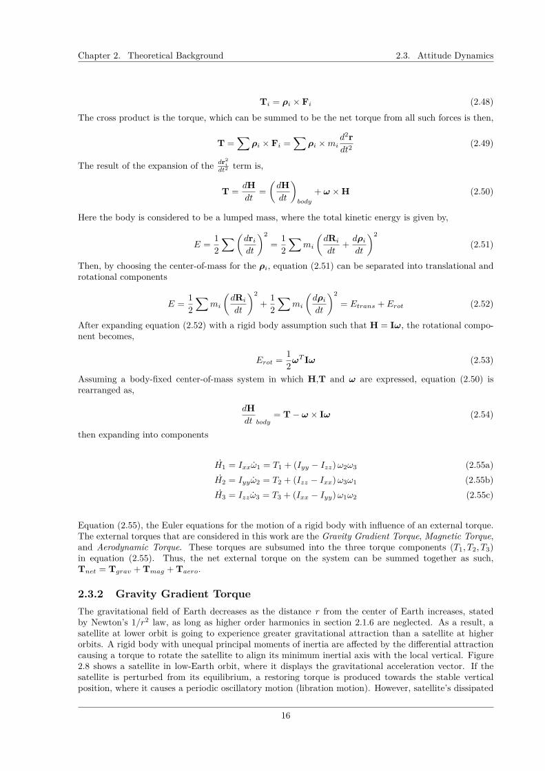
Equation (2.55), the Euler equations for the motion of a rigid body with influence of an external torque.The external torques that are considered in this work are the Gravity Gradient Torque, Magnetic Torque,and Aerodynamic Torque. These torques are subsumed into the three torque components (T1, T2, T3)in equation (2.55). Thus, the net external torque on the system can be summed together as such,Tnet = Tgrav + Tmag + Taero.
2.3.2 Gravity Gradient TorqueThe gravitational field of Earth decreases as the distance r from the center of Earth increases, statedby Newton’s 1/r2 law, as long as higher order harmonics in section 2.1.6 are neglected. As a result, asatellite at lower orbit is going to experience greater gravitational attraction than a satellite at higherorbits. A rigid body with unequal principal moments of inertia are affected by the differential attractioncausing a torque to rotate the satellite to align its minimum inertial axis with the local vertical. Figure2.8 shows a satellite in low-Earth orbit, where it displays the gravitational acceleration vector. If thesatellite is perturbed from its equilibrium, a restoring torque is produced towards the stable verticalposition, where it causes a periodic oscillatory motion (libration motion). However, satellite’s dissipated
16

Chapter 2. Theoretical Background 2.3. Attitude Dynamics
energy will damp this motion [7].
The gravity gradient torque for a satellite is given by,
Tgrav =∫
r× agdm (2.56)
where the gravitational acceleration, ag, is
ag = −µ R + r|R + r|3 (2.57)
Here µ is the Earth’s gravitational parameter (3.98601 × 10⁵ km3/s2), R is the center of mass of thesatellite with respect to Earth.
Figure 2.8: Gravity gradient torques on a low-Earth orbit satellite. [8]
To subsume the torque Tgrav in Euler’s equation, the integral (2.56) is evaluated in the principal-axisbody frame. Here let the components R = [R1, R2, R3] be in the body frame and the componentsr = [r1, r2, r3]. Then develop equation (2.56), as in Wiesel, W [8], the gravity gradient torque becomes,
Tgrav = 3µR5 R× IR (2.58)
I is the principal moments of inertia. The torque components are then separately written in the body-fixedframe,
Tgrav1 = 3µR5R2R3 (Izz − Iyy) (2.59a)
Tgrav2 = 3µR5R1R3 (Ixx − Izz) (2.59b)
Tgrav3 = 3µR5R1R2 (Iyy − Ixx) (2.59c)
Observing equations (2.59), it is good to note that only an asymmetrical body will experience gravitationaltorque due to the difference in principal moment of inertia.
2.3.3 Magnetic TorqueThe Earth’s magnetic field is another torque that is exerted on to the satellite in low-Earth orbits. Thistorque is given by,
Tmag = M×B (2.60)where M is the magnetic dipole moment due to current loops and residual magnetization in the satellite.B is the Earth magnetic field vector that is expressed in body-fixed coordinates. The magnitude isproportional to 1/r3, where r is the radius vector from the center of Earth to the satellite.
17

Chapter 2. Theoretical Background 2.3. Attitude Dynamics
2.3.4 Aerodynamic TorqueThe effect of the upper atmosphere on the satellite decay was discussed in section 2.1.5. The same dragforce also produces a disturbance torque on the satellite due to any offsets between the aerodynamiccenter of pressure and the center of mass. The aerodynamic torque is written as,
Taero = rcp × Faero (2.61)
where rcp is the center-of-pressure (CP) vector in body-fixed coordinates and Faero is the aerodynamicforce applied. Here, the aerodynamic force is the mass of the satellite multiplied by the same dragacceleration in section 2.1.5. Further expansion of aerodynamic torque will be discussed later in section4.2.2, where partial accommodation of incoming particles are considered.
18

Chapter 3
Orbital Decay
In order to investigate the orbital decay, the Earth atmosphere must first be examined since aerodynamicdrag is the main cause of decay. Satellites in low earth orbits still encounter drag, lift, heating andexperience orbit decay as a consequence of passing through the upper atmosphere. At higher altitudessuch as 600 km, the perturbations in the orbital period are so minute that the drag can simply be takeninto consideration without accurate knowledge of the atmosphere [2]. At intermediate altitudes, to be ableto predict variations in the atmospheric density and generate orbit perturbations, atmospheric modelsneed to be examined.
3.1 Comparing Atmospheric ModelsThe two empirical models used to predict the densities and temperatures of the Earth’s thermosphere(90 to about 600 km altitude) are the Jacchia J70 model and the US Naval Research Laboratory MassSpectrometer Incoherent Scatter Radar Exosphere 2000 (NRLMSISE-00). Both models discussed inthis section use similar input parameters. These parameters include time of day, day of year, altitudeand geographic location of the satellite. The density variations are also expressed terms of solar andgeomagnetic activity indices, such as the 10.7 cm solar flux (F10.7 index) and the Ap for geomagneticactivity. The inputs used in both atmospheric models are shown in table 3.1.
F10.7 index (Maximum) = 225F10.7 index (Minimum) = 75Average Ap index (Maximum) = 20Average Ap index (Minimum) = 8
Table 3.1: Atmospheric model input parameters.
3.1.1 Jacchia J70 ModelThe Jacchia models are based on satellite drag data collected from ground-based tracking of selectedsatellites [14]. The altitude of the model ranges from 90 to 2500 km, and the exospheric temperaturesrange from 600 to 2000 K. Any altitude below 90 km uses the standard atmosphere to estimate thedensity and temperature. It is important to note that during the time when the model was made, goodobservational data did not exist above 1100 km. Hence, all the output above the height are consideredto be unconfirmed extrapolation [14]. The model’s prediction method is derived from the static diffusionmodel, where it defines temperature and chemical composition. The diffusion model provides densitiesthat correspond with satellite drag observations, with rocket probe measurements [15].
In order to determine the variability of the Jacchia J70 model, the model is tested with different seasons,
19
Chapter 3. Orbital Decay 3.1. Comparing Atmospheric Models
latitudes and solar activities. Figure 3.1 shows density maps comparing several months during high andlow solar activity. As discussed above while it is important to see the density variation between differ-ent solar activity conditions, it is also significant to understand the variations between local solar time.Figure 3.1, shows the variations from night to day. The density variation on the daytime can be 3 timeshigher than the nighttime, during solar maximum. However, the dramatic variations in the density arelower during solar minimum, with only the daytime density being about one and a half times higher thanthe nighttime.
20

Chapter 3. Orbital Decay 3.1. Comparing Atmospheric Models
(a) Density map: September with high solar activity. (b) Density map: September with low solar activity.
(c) Density map: January with high solar activity. (d) Density map: January with low solar activity.
(e) Density map: May with high solar activity. (f) Density map: May with low solar activity.
Figure 3.1: J70: Density maps at 300 km altitude of 3 months showing high and solar activity conditions.
Figure 3.2 provides a density ratio map by dividing the solar maximum over the solar minimum forvarious altitudes and latitudes of different seasons (September, January, May). For the same seasons,figure 3.3 shows the atmospheric density as a function of altitude for solar maximum and solar minimum
21

Chapter 3. Orbital Decay 3.1. Comparing Atmospheric Models
conditions. During the summer months (September and May) a higher variability with solar activity isobserved. At altitudes of approximately 150 km, the solar activity does not strongly affect the density asseen in figure 3.3. However, at higher altitudes such as 500-800 km, the density varies approximately 2 to3 orders of magnitude between solar minimum and solar maximum. The order of magnitude is significantbecause the density variations would affect the satellite drag, which leads to a faster decay during theperiod of solar maximum.
(a) September (b) January
(c) May
Figure 3.2: J70: Density map of the solar maximum-minimum ratio for different altitudes and latitudesof different months.
22

Chapter 3. Orbital Decay 3.1. Comparing Atmospheric Models
(a) September (b) January
(c) May
Figure 3.3: J70: Log10 of density as a function of altitude for solar maximum and solar minimum atdifferent months.
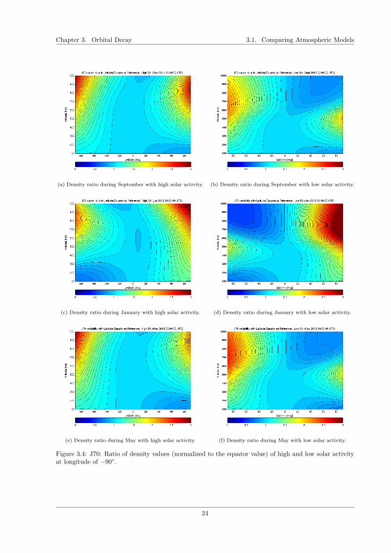
Figure 3.4 shows the variation of density profile normalized to the equatorial value. The densities areup to three times the equatorial value in the polar regions. However, the densities at the polar regionsare lower during solar minimum, compared to the density ratio during solar maximum, for the monthsSeptember and May. This shows that the density is dependent on latitude and season. At altitude of 200km, density in the polar regions are 15% greater than the equatorial region during the summer season.On the contrary, at the same altitude there is a 10% decrease in the polar region density during thewinter. These observations of the model are in agreement with the statement in Newton and Pelz, thata weak dependency of density on latitude and season exists such that in summer at 200 km height thepolar region density is 15% higher than lower altitudes, whereas in winter the density decreased by 10%[16]. In addition, large density ratios (> 3) are observed only near the polar regions, both during solarmaximum and solar minimum.
23
Chapter 3. Orbital Decay 3.1. Comparing Atmospheric Models
(a) Density ratio during September with high solar activity. (b) Density ratio during September with low solar activity.
(c) Density ratio during January with high solar activity. (d) Density ratio during January with low solar activity.
(e) Density ratio during May with high solar activity. (f) Density ratio during May with low solar activity.
Figure 3.4: J70: Ratio of density values (normalized to the equator value) of high and low solar activityat longitude of −90.
24
Chapter 3. Orbital Decay 3.1. Comparing Atmospheric Models
3.1.2 NRLMSISE-00 ModelThe NRLMSISE-00 (Mass Spectrometer and Incoherent Scatter Radar Extended) model is an empiricaldensity model, developed by the US Naval Research Laboratory, based on the MSISE-90 model. TheNRLMSISE-00 model finds the total density by taking into account the contributions of N2, O, O2,He, Ar and H. The satellite total mass density data are from satellite accelerometers and from orbitdetermination (including Jacchia data), where it is valid from 0 to 1000 km. The incoherent scatter dataprovide the temperature and the molecular number oxygen density is from solar ultraviolet occultationaboard the Solar Maximum Mission [14]. The major differences between the NRLMSISE-00 model andthe MSISE-90 model are: (1) the total mass density uses the drag and accelerometer data extensively,including Jacchia and Barlier data sets. (2) at altitudes above 500 km, the total mass density accountsfor large contributions from O+ and hot oxygen. (3) the SSM UV occultation data on O2 are included.(4) the temperature data from incoherent scatter data covers 1981-1997 [17][18].
The density variations as the satellite passes from the nighttime to daytime are represented in figure3.5. During solar maximum, the daytime density is 3 times greater than the nighttime, which is similarto the Jacchia J70 model in figure 3.1. As for the variation during solar minimum, the daytime-nighttimevariations are less, with the exception of the variation in the month of September. In September thedensity is a magnitude less than the months of January and May. During the months of January andMay, the daytime density is 0.8 times greater than the nighttime. The NRLMSISE-00 model’s nighttime-daytime density variations are unevenly distributed with respect to the latitudes compared to the JacchiaJ70 model. A reason for this might be due to the NRLMSISE-00 model’s inclusion of numerous satellitedrag and accelerometer data [18].
25

Chapter 3. Orbital Decay 3.1. Comparing Atmospheric Models
(a) Density map: September with high solar activity. (b) Density map: September with low solar activity.
(c) Density map: January with high solar activity. (d) Density map: January with low solar activity.
(e) Density map: May with high solar activity. (f) Density map: May with low solar activity.
Figure 3.5: NRLMSISE-00: Density maps at 300 km altitude of 4 months showing high and low solaractivity conditions.
The density ratio map of the NRLMSISE-00 are shown in figure 3.6, where the density at solar maximumis divided by density at solar minimum conditions. These values are plotted for different altitudes,
26

Chapter 3. Orbital Decay 3.1. Comparing Atmospheric Models
latitudes and seasons. In figure 3.6 the NRLMSISE-00 model shows an agreement with the Jacchia J70model, that there is a greater variability with solar activity in the North Pole than the South Pole duringthe summer. Further, figure 3.7 shows the variability of the density during high and low solar activity.The density between solar maximum and solar minimum diverges at altitudes greater than 150 km. Itis observed that at the altitude of 600 km, there is a density difference of 3 orders of magnitude betweenthe solar maximum and solar minimum.
(a) September (b) January
(c) May
Figure 3.6: NRLMSISE-00: Density map of the solar maximum-minimum ratio for different altitudesand latitudes of different months.
27
Chapter 3. Orbital Decay 3.1. Comparing Atmospheric Models
(a) September (b) January
(c) May
Figure 3.7: NRLMSISE-00: Log10 of density as a function of altitude for solar maximum and solarminimum at different months.
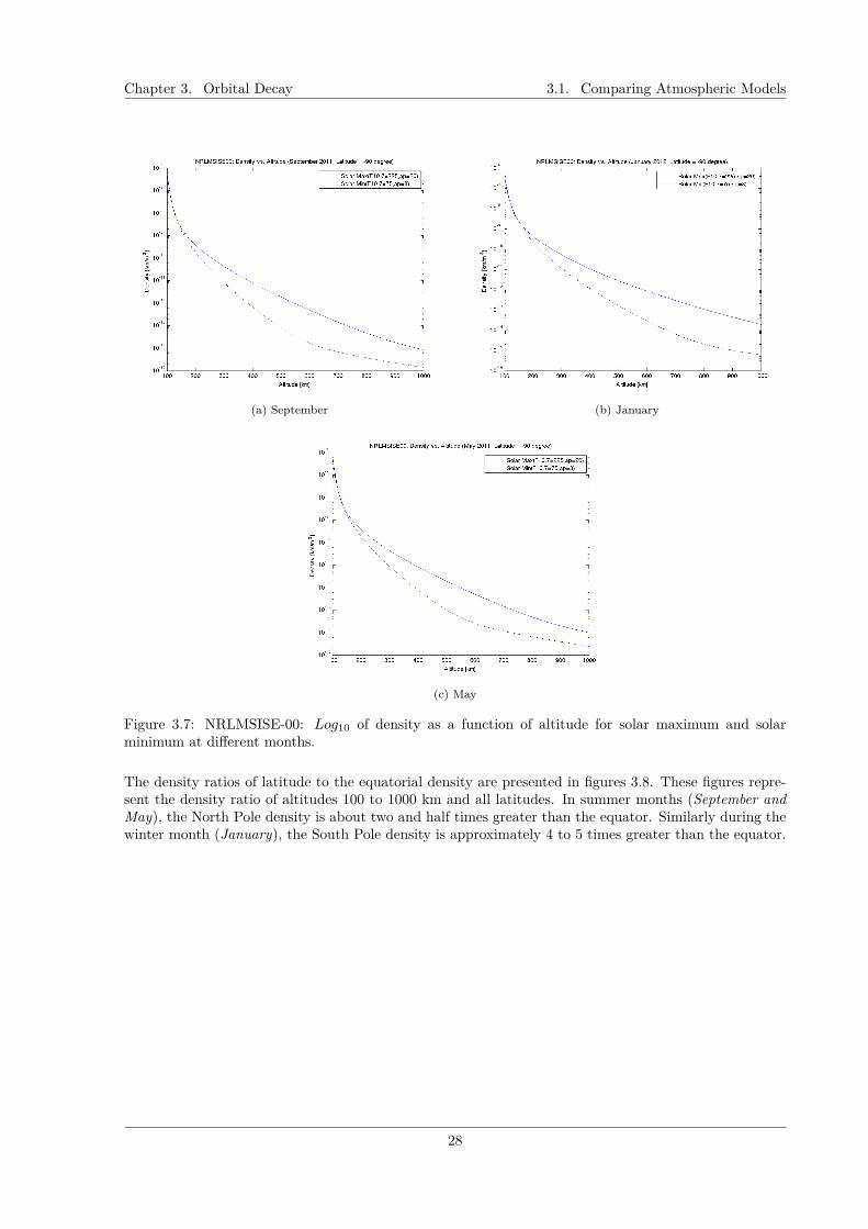
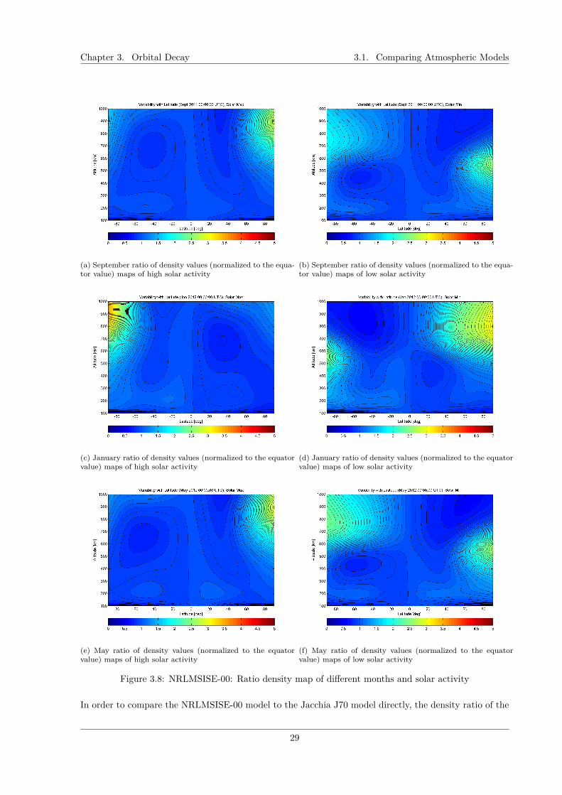
The density ratios of latitude to the equatorial density are presented in figures 3.8. These figures repre-sent the density ratio of altitudes 100 to 1000 km and all latitudes. In summer months (September andMay), the North Pole density is about two and half times greater than the equator. Similarly during thewinter month (January), the South Pole density is approximately 4 to 5 times greater than the equator.
28
Chapter 3. Orbital Decay 3.1. Comparing Atmospheric Models
(a) September ratio of density values (normalized to the equa-tor value) maps of high solar activity
(b) September ratio of density values (normalized to the equa-tor value) maps of low solar activity
(c) January ratio of density values (normalized to the equatorvalue) maps of high solar activity
(d) January ratio of density values (normalized to the equatorvalue) maps of low solar activity
(e) May ratio of density values (normalized to the equatorvalue) maps of high solar activity
(f) May ratio of density values (normalized to the equatorvalue) maps of low solar activity
Figure 3.8: NRLMSISE-00: Ratio density map of different months and solar activity
In order to compare the NRLMSISE-00 model to the Jacchia J70 model directly, the density ratio of the
29

Chapter 3. Orbital Decay 3.1. Comparing Atmospheric Models
two models are plotted in figure 3.9. The regions that the NRLMSISE-00 show significant differencesare the North and South Poles. At solar minimum, the NRLMSISE-00 density is two times greater thanthe J70 model, at approximately 600 km altitude. However, at solar maximum, the Jacchia J70 model’sNorth Pole density is greater than the NRLMSISE-00 at altitudes of 1000 km. This is observed in figure3.9.
30

Chapter 3. Orbital Decay 3.1. Comparing Atmospheric Models
(a) Density ratio during September with high solar activity. (b) Density ratio during September with low solar activity.
(c) Density ratio January with high solar activity. (d) Density ratio during January with low solar activity.
(e) Density ratio during May with high solar activity. (f) Density ratio during May with low solar activity.
Figure 3.9: Density ratio between NRLMSISE-00 over J70.
31

Chapter 3. Orbital Decay 3.1. Comparing Atmospheric Models
3.1.3 Summary of Atmospheric ModelsJacchia J70 Model: The Jacchia J70 model’s altitude ranges from 0 km to 2,500 km, where thestandard atmospheric model is used at altitudes below 90 km. The density is found to be dependent onlatitude, season and solar activity.
1. Density variation due to local time at 300 km altitude.
(a) The daytime density is 3 times greater than the night time density during solar maximum.(b) During solar minimum, the daytime density is 1.5 times greater than the nighttime density.
2. Density variation due to solar activity.
(a) Solar activity does not affect the density below the altitude of 150 km.(b) A density difference of 2 to 3 orders of magnitude are noticed at altitudes of 500-800 km.
3. Density variation due to latitude.
(a) During the summer months, the density in the polar regions are 15% greater than the equatorialregion.
(b) During the winter month, the density in the polar regions decrease by approximately 10%compared to the equatorial regions.
NRLMSISE-00: The NRLMSISE-00 model’s altitude ranges from 0 km to 1,000 km. The density inthis model is also dependent on latitude, season and solar activity.
1. Density variation due to local time at 300 km altitude.
(a) During solar maximum, daytime density is 3 times greater than the nighttime.(b) For September during solar minimum, the daytime density is a magnitude lower than the
daytime density of January and May.(c) For January and May, during solar minimum, the daytime density is approximately 0.8 times
greater than the nighttime density.
2. Density variation due to solar activity.
(a) The solar activity does not affect the density at altitudes lower than 150 km.(b) Solar maximum and minimum affects the density at altitudes above 600 km, where there are
density differences up to 3 orders of magnitude.
3. Density variation due to latitude.
(a) The North Pole density during solar maximum is approximately 2.5 times greather than theequatorial value.
(b) The South Pole density during solar maximum is approximately 4 to 5 times greater than theequatorial value.
(c) During solar minimum, the density variations happen both in the North Pole as well as theSouth Pole.
Even though the range of altitude covered by the Jacchia J70 model is greater, the detail of the densityvariations in the NRLMSISE-00 model is greater. Additionally, the NRLMSISE-00 also includes numeroussatellite drag and accelerometer data on total mass density. Hence, the NRLMSISE-00 is more suitablefor this work since the analysis of the satellite extensively uses atmospheric density.
32
Chapter 3. Orbital Decay 3.2. Decay Lifetime Simulation
3.2 Decay Lifetime SimulationLow-Earth orbit satellites have a finite lifetime due to the effects of atmospheric drag. The effects ofdrag are cumulative and eventually become significant; therefore, it is necessary to understand theseeffects in order to determine the lifetime of the satellite. Here, simulations are run using different ballisticcoefficients,
CBallistic = M
Cd ·A(3.1)
where M is the mass of the satellite, Cd is the coefficient of drag, and A is the ram-facing area. First,effects of atmospheric drag is analyzed, then the effect of Earth oblateness is added. As a result, byperforming the decay lifetime simulations, an appropriate altitude for orbit insertion can be determined.
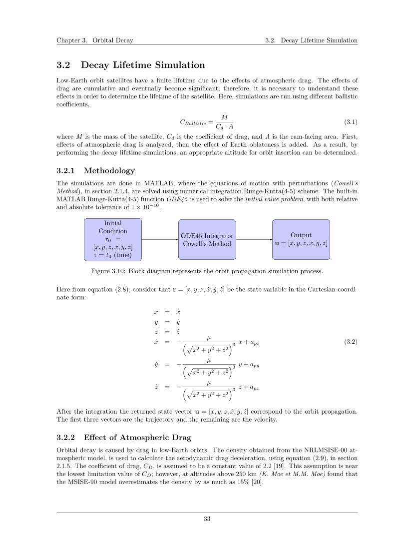
3.2.1 MethodologyThe simulations are done in MATLAB, where the equations of motion with perturbations (Cowell’sMethod), in section 2.1.4, are solved using numerical integration Runge-Kutta(4-5) scheme. The built-inMATLAB Runge-Kutta(4-5) function ODE45 is used to solve the initial value problem, with both relativeand absolute tolerance of 1× 10⁻¹⁰.
InitialCondition
r0 =[x, y, z, x, y, z]t = t0 (time)
ODE45 IntegratorCowell’s Method
Outputu = [x, y, z, x, y, z]
Figure 3.10: Block diagram represents the orbit propagation simulation process.
Here from equation (2.8), consider that r = [x, y, z, x, y, z] be the state-variable in the Cartesian coordi-nate form:
x = x
y = y
z = z
x = − µ(√x2 + y2 + z2
)3 x+ apx (3.2)
y = − µ(√x2 + y2 + z2
)3 y + apy
z = − µ(√x2 + y2 + z2
)3 z + apz
After the integration the returned state vector u = [x, y, z, x, y, z] correspond to the orbit propagation.The first three vectors are the trajectory and the remaining are the velocity.
3.2.2 Effect of Atmospheric DragOrbital decay is caused by drag in low-Earth orbits. The density obtained from the NRLMSISE-00 at-mospheric model, is used to calculate the aerodynamic drag deceleration, using equation (2.9), in section2.1.5. The coefficient of drag, CD, is assumed to be a constant value of 2.2 [19]. This assumption is nearthe lowest limitation value of CD; however, at altitudes above 250 km (K. Moe et M.M. Moe) found thatthe MSISE-90 model overestimates the density by as much as 15% [20].
33

Chapter 3. Orbital Decay 3.2. Decay Lifetime Simulation
The influence of the upper atmosphere on the satellite is simulated for different perigees. These sim-ulations are done at orbits with apogee of 6000 km and perigees of 190 km, 170 km, and 150 km. Theacceleration due to drag is added to the equations of motion in section 2.1.4. Table 3.2 presents the initialconditions for the orbital decay simulation.
Apogee a = 6000 kmPerigee p = 150 km, 170 km, 190 kmInclination i = 90True anomaly θ = 0Right ascension of the ascending node Ω = 0 Argument of perigee ω = 0 Mass m = 3 kgRam facing area A = 0.1 m2
Table 3.2: Initial orbital decay conditions.
Simulations are run for orbital decays with a lifetime of 3 months. As expected, the lower the initialperigee the faster the decay time. In figure 3.11, the simulation of Perigee = 150 km, de-orbits beforethe 3 months. The simulations that start at Perigee = 170 km and Perigee = 190 km, does not de-orbitin 3 months. This shows the influence of atmospheric density on the rate of orbit decay.
Figure 3.11: Orbital Decay due to aerodynamic drag.
3.2.3 Effect of J2 PerturbationAtmospheric drag is not the only perturbation that affects the satellite in low-Earth orbits. As mentionedearlier in section 2.1.6, Earth oblateness is a crucial perturbation to subsume into the equations of motion.Simulations are run for the same initial conditions as in section 3.2.2, for initial perigees of 170 km and190 km.
34

Chapter 3. Orbital Decay 3.2. Decay Lifetime Simulation
Figure 3.12: Orbital Decay due to drag and Earth oblateness.
The effects of the Earth oblateness are the oscillations in the decay. This is evident in figure 3.12, whereit shows both decay with and without Earth oblateness perturbation. Additionally, the orbit decay timeis also affected by the Earth oblateness. Figure 3.13, compares different inclinations to show the causeof the oscillations. The orbit decay trajectory with zero inclination does not have any oscillations incontrast to the orbit trajectories with 30, and 90 inclination. Then from the comparison, it is clear theoscillations are prominent due to the 90 inclination of the orbit.
Figure 3.13: Earth oblateness effect on different orbit inclinations.
The appropriate range of insertion altitudes are found using an iterative method. The range of altitudesare narrowed down from 150-190 km to approximately 160-170 km, by observing the decay time of eachperigee insertion. The iterative results are shown in figure 3.14, where the appropriate perigee insertionof the satellite should be between 165-170 km.
35
Chapter 3. Orbital Decay 3.2. Decay Lifetime Simulation
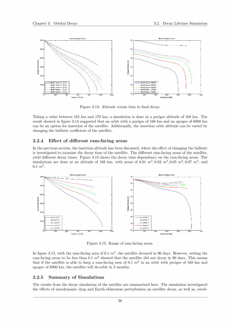
Figure 3.14: Altitude versus time in final decay.
Taking a value between 165 km and 170 km, a simulation is done at a perigee altitude of 168 km. Theresult showed in figure 3.14 suggested that an orbit with a perigee of 168 km and an apogee of 6000 kmcan be an option for insertion of the satellite. Additionally, the insertion orbit altitude can be varied bychanging the ballistic coefficient of the satellite.
3.2.4 Effect of different ram-facing areasIn the previous section, the insertion altitude has been discussed, where the effect of changing the ballisticis investigated to examine the decay time of the satellite. The different ram-facing areas of the satellite,yield different decay times. Figure 3.15 shows the decay time dependency on the ram-facing areas. Thesimulations are done at an altitude of 168 km, with areas of 0.01 m2, 0.03 m2, 0.05 m2, 0.07 m2, and0.1 m2.
Figure 3.15: Range of ram-facing areas.
In figure 3.15, with the ram-facing area of 0.1 m2, the satellite decayed in 90 days. However, setting theram-facing areas to be less than 0.1 m2 showed that the satellite did not decay in 90 days. This meansthat if the satellite is able to keep a ram-facing area of 0.1 m2 in an orbit with perigee of 168 km andapogee of 6000 km, the satellite will de-orbit in 3 months.
3.2.5 Summary of SimulationsThe results from the decay simulation of the satellite are summarized here. The simulation investigatedthe effects of aerodynamic drag and Earth-oblateness perturbation on satellite decay, as well as, estab-
36
Chapter 3. Orbital Decay 3.2. Decay Lifetime Simulation
lished a possible insertion orbit. In addition, the effect of changing the ballistic coefficients by means ofvarying the ram-facing area is also examined.
The results indicated that an appropriate insertion orbit for the satellite is around perigee of 168 km andapogee of 6000 km, to be able to de-orbit in 90 days. However, this is quite ideal since the satellite wouldhave to keep a constant ram-facing area of 0.1 m2 as showed later in section 3.2.4. In addition, due tothe high inclination orbit required for the mission, the effect of Earth oblateness perturbation influencesthe satellite’s trajectory as seen in section 3.2.3.
37

Chapter 4
Satellite Attitude Simulation
In low-Earth-orbits, satellites are subjected to many different forces that affect its attitude and stability.This chapter studies the feasibility of using aerodynamic drag panels as a mean of decelerating the satelliteduring the perigee pass. As seen in section 3.2.4, having a certain ballistic coefficient, the satellite is ableto decelerate and reduce its apogee. Existing literature proposes the combined use of aerodynamic andmagnetic torquing, to achieve three axis attitude control [21]. In addition, building on previous workthat used gravity gradient stabilization and magnetic torquing [12], a drag panel is added to the satelliteconfiguration. The analysis in this chapter aims to provide an understanding of aerodynamic torque oneach principal axis.
4.1 Satellite GeometryAccording to section 3.2.4, a constant ram-surface area of 0.1 m2 allows the satellite to decay in threemonths. In order to adhere to the compact requirements of a CubeSat, a deployable panel is positionedat a certain angle once the satellite is in orbit. The CubeSat configuration in this section is an attemptto understand the behavior of using aerodynamic drag as means of orbit, attitude control, and formationmaintenance. A specific geometry of a 3U-CubeSat is established consisting of a control panel placed tothe rear of the center of gravity. An idea taken from a badminton shuttlecock, the panel provides passivestability about the pitch axis. Additionally, a mass constraint of ≤ 4 kg is put on the satellite.
Figure 4.1: Satellite geometry isometric view.
38
Chapter 4. Satellite Attitude Simulation 4.1. Satellite Geometry
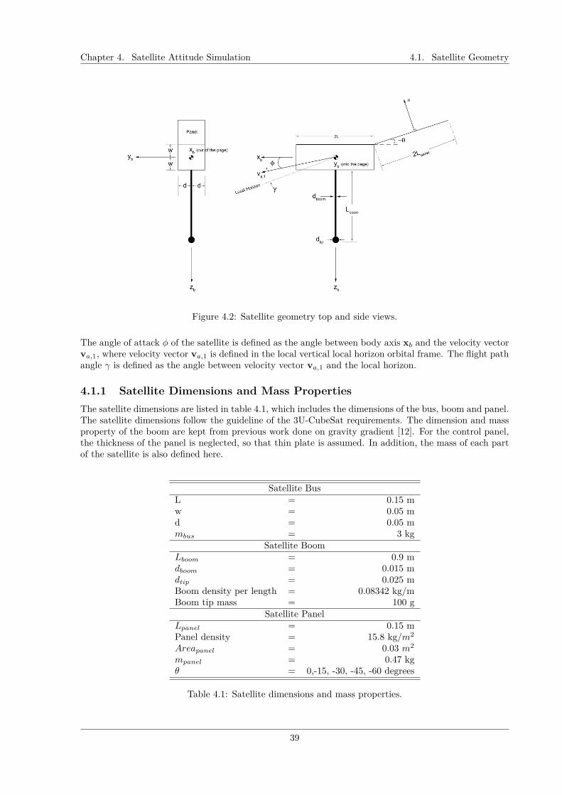
Figure 4.2: Satellite geometry top and side views.
The angle of attack φ of the satellite is defined as the angle between body axis xb and the velocity vectorva,1, where velocity vector va,1 is defined in the local vertical local horizon orbital frame. The flight pathangle γ is defined as the angle between velocity vector va,1 and the local horizon.
4.1.1 Satellite Dimensions and Mass PropertiesThe satellite dimensions are listed in table 4.1, which includes the dimensions of the bus, boom and panel.The satellite dimensions follow the guideline of the 3U-CubeSat requirements. The dimension and massproperty of the boom are kept from previous work done on gravity gradient [12]. For the control panel,the thickness of the panel is neglected, so that thin plate is assumed. In addition, the mass of each partof the satellite is also defined here.
Satellite BusL = 0.15 mw = 0.05 md = 0.05 mmbus = 3 kg
Satellite BoomLboom = 0.9 mdboom = 0.015 mdtip = 0.025 mBoom density per length = 0.08342 kg/mBoom tip mass = 100 g
Satellite PanelLpanel = 0.15 mPanel density = 15.8 kg/m2
Areapanel = 0.03 m2
mpanel = 0.47 kgθ = 0,-15, -30, -45, -60 degrees
Table 4.1: Satellite dimensions and mass properties.
39

Chapter 4. Satellite Attitude Simulation 4.1. Satellite Geometry
4.1.2 Center of GravityThe knowledge of a rigid body’s center of mass is vital, since the attitude control takes place around thecenter of mass. The center of mass is calculated by,
Rc.m. = 1M
∑miri (4.1)
where Rc.m. is the center of mass, M is M is the total mass of the system of particles, ri is the averageposition of particle i, and mi is the mass of particle i.
The center of mass of each components of the satellite are listed in Table 4.2, where it is good tonote that the center of mass changes as the control panel angle changes.
Element Mass Rc.m,1 Rc.m,2 Rc.m,3Bus mbus 0 0 0Boom mboom l 0 Lboom/2Tip mtip l 0 LPanel mpanel − (d+ Lpanelcosθ) 0 − (w + wpanelsinθ)
Table 4.2: Location of the satellite center of mass.
4.1.3 Principal Moments of InertiaThe principle moments of inertia stated in equation are used in the calculation of angular momentumin section section:RotDynamics. The moment of inertia dictates rotation around the body axes, whichare computed based on the knowledge of component mass and location. The equation for the moment ofinertia is stated as,
Ii =∑
r2imi (4.2)
where Ii is the is the moment of inertia, ri is the position vector and mi is the mass. Since the momentof inertia matrix is symmetric, the vectors ωi corresponding to the three Ii are perpendicular. There-fore, there are only three possible axes in the rigid body about which angular momentum H and ω areparallel. The three special Ii are the diagonal terms of the moment of inertia matrix, which are termedthe principal moments of inertia. While the corresponding ωi are called the principal moments of inertia[8]. The principal moments of inertia of each satellite component are shown in Table 4.3.
Element Mass I1 I2 I3Bus mbus
mbus
12(4d2 + 4w2) mbus
12(4d2 + 4L2) mbus
12(4w2 + 4L2)
Boom mboommboom
12 L2boom
mboom12 L2
boom 0Tip mtip 0 0 0Panel mpanel 0 0 mpanel
12
(4w2
panel + 4L2panel
)Table 4.3: The principal moments of inertia of the satellite.
As the origin of the body frame changes, it is important to know how the moment of inertia matrixchanges. Hence the parallel axis theorem gives the moment of inertia matrix about a new origin. Thenew principal moments of inertia are given by,
I = I +md2 (4.3)
40

Chapter 4. Satellite Attitude Simulation 4.2. Attitude Simulation
where I is the principal moments of inertia for a parallel axis, I is the moment of inertia at the centerof mass, m is the mass of the element and d is the distance of the parallel axis. The final moments ofinertia used in the calculations are stated,
I1 = mbus
12(4d2 + 4w2)+mbusd
21,bus + mboom
12 L2boom +mboomd
21,boom +mtipd
2tip,1
+mpaneld23,panel
I2 = mbus
12(4d2 + 4L2)+mbusd
22,bus + mboom
12 L2boom +mboomd
22,boom +mtipd
2tip,2
+mpaneld23,panel
I3 = mbus
12(4w2 + 4L2)+mbusd
23,bus +mboomd
23,boom +mtipd
2tip,3 + mpanel
12(4w2
panel + 4L2panel
)+mpaneld
23,panel
(4.4)
4.2 Attitude SimulationThe attitude simulation in this section combines orbital mechanics with satellite dynamics and kinematics.The simulation includes external torques; therefore, it is important to calculate the aerodynamic torqueprofiles over different attitude angles for roll, pitch and yaw axes. The torque profiles are plotted forattitude angles during the perigee passage, where they are established for attitude angles of -90 to 90degrees, and all principle axes. Then the torque profiles are calculated for true anomalies, ν = 0 andν = 270, which represents the perigee passage of the satellite. In addition, different panel settings havealso been taken into consideration. Since different panel angles produce different torques, the panel istested for angles 0, -15, -30, -45 and -60 degrees. Furthermore, the aerodynamic shadowing by the ramsurface reduces the drag effects on the control panel. Hence, the aerodynamic shadowing is modeled bysetting the length of the shadowed panel to zero.
4.2.1 Attitude PropagationIn order to estimate the satellite’s behavior due to external torques, a simulation is done with the sameequations in section 3.2 for the position and velocity are considered. Taking r to be r = (x, y, z) thenthe state variables are in the form,
x = x
y = y
z = z
x = − µ(√x2 + y2 + z2
)3 x+ apx
y = − µ(√x2 + y2 + z2
)3 y + apy
z = − µ(√x2 + y2 + z2
)3 z + apz
(4.5)
Likewise, the Euler equations of motion for a rigid body from section 2.3 are rewritten in state-variableform,
41
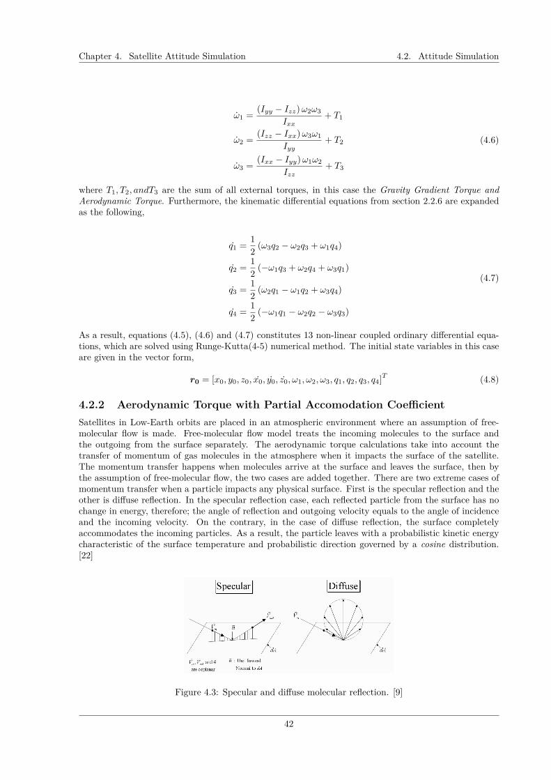
Chapter 4. Satellite Attitude Simulation 4.2. Attitude Simulation
ω1 = (Iyy − Izz)ω2ω3
Ixx+ T1
ω2 = (Izz − Ixx)ω3ω1
Iyy+ T2
ω3 = (Ixx − Iyy)ω1ω2
Izz+ T3
(4.6)
where T1, T2, andT3 are the sum of all external torques, in this case the Gravity Gradient Torque andAerodynamic Torque. Furthermore, the kinematic differential equations from section 2.2.6 are expandedas the following,
q1 = 12 (ω3q2 − ω2q3 + ω1q4)
q2 = 12 (−ω1q3 + ω2q4 + ω3q1)
q3 = 12 (ω2q1 − ω1q2 + ω3q4)
q4 = 12 (−ω1q1 − ω2q2 − ω3q3)
(4.7)
As a result, equations (4.5), (4.6) and (4.7) constitutes 13 non-linear coupled ordinary differential equa-tions, which are solved using Runge-Kutta(4-5) numerical method. The initial state variables in this caseare given in the vector form,
r0 = [x0, y0, z0, x0, y0, z0, ω1, ω2, ω3, q1, q2, q3, q4]T (4.8)
4.2.2 Aerodynamic Torque with Partial Accomodation CoefficientSatellites in Low-Earth orbits are placed in an atmospheric environment where an assumption of free-molecular flow is made. Free-molecular flow model treats the incoming molecules to the surface andthe outgoing from the surface separately. The aerodynamic torque calculations take into account thetransfer of momentum of gas molecules in the atmosphere when it impacts the surface of the satellite.The momentum transfer happens when molecules arrive at the surface and leaves the surface, then bythe assumption of free-molecular flow, the two cases are added together. There are two extreme cases ofmomentum transfer when a particle impacts any physical surface. First is the specular reflection and theother is diffuse reflection. In the specular reflection case, each reflected particle from the surface has nochange in energy, therefore; the angle of reflection and outgoing velocity equals to the angle of incidenceand the incoming velocity. On the contrary, in the case of diffuse reflection, the surface completelyaccommodates the incoming particles. As a result, the particle leaves with a probabilistic kinetic energycharacteristic of the surface temperature and probabilistic direction governed by a cosine distribution.[22]
Figure 4.3: Specular and diffuse molecular reflection. [9]
42

Chapter 4. Satellite Attitude Simulation 4.2. Attitude Simulation
Figure 4.3, represents the two concepts of specular and diffuse molecular reflection. In regards of the twocases of specular and diffuse molecular reflection, a reasonable assumption lies somewhere between thetwo. The particle at least becomes partially accommodated by the surface but not totally accommodated.The analysis of aerodynamic torque in this work assumes partial surface accommodation of the incomingparticles.
Based on partial surface accommodation, the force and torque expressions are derived to include themomentum of molecules leaving the surface. Figure 4.4, shows the force acting on the satellite surface(dA).
Figure 4.4: Molecules incident on an element of the satellite surface. [9]
The force acting on the surface (dA) by the local atmosphere are decomposed into inward facing normalcomponent (n) and a tangential component (t). As a result, the force components follow the samedecomposition, having a normal component (dFn) and a tangential component (dFt). Trivially, summingthe normal and tangential components, the force acting on (dA) is written as such:
dF = dFn + dFt (4.9)Through the assumption that the mean thermal motion of the atmosphere is much smaller than the speedof the satellite through the atmosphere, the incoming atmosphere is viewed as a parallel molecular beamof density (ρ) and velocity VR. As seen in figure 4.4, let V = VR
|VR| and n be the unit inward normal tothe surface of (dA) [22].
cos α = VR · n (4.10)where the velocity vector VR is in the body frame of the satellite moving in Earth’s atmosphere, and nis the vector normal to the plane. The velocity vector is described by,
VR = Vi ·RBN (4.11)where Vi is the velocity vector in the inertial frame and RBN is the transformation matrix from theinertial frame to the body frame.
The angle of incidence (α) is the angle which the particle impacts the surface of the satellite, and iscalculated by equation (4.10). The projected area acted upon by local atmosphere is (dA cos α) in thenormal direction and (dA sin α) in the tangential direction. The molecular momentum flux through(dA cos α) is a force imparted to (dA) [22] [9]. Hence, the force is written as:
dF = ρ V 2R cosα VR dA + ρ V 2
R sinα VR dA (4.12)where ρ is the local atmospheric density.
43

Chapter 4. Satellite Attitude Simulation 4.2. Attitude Simulation
When the satellite travels through space, it is good to note that not all surfaces will impact the up-per atmosphere. Thus, if cosα ≥ 0 then that element is exposed to the flow. On the contrary, if cosα < 0then that element is shadowed from the flow. Consequently, using the Heaviside function, H(·), the con-ditions above are then accounted for in the force and torque calculations [9]. For example, if cosα ≥ 0,then H(cosα) = 1, and if cosα < 0, H(cosα) = 0.
Incorporating the Heaviside function into the equation (4.12), the force expressions for normal and tan-gential components for diffuse reflection becomes,
dfDiffusen = H(cosα)ρVRcosα[VRcosα+ Vb]ndA (4.13)
dfDiffuset = H(cosα)ρV 2RsinαcosαtdA (4.14)
where Vs is the molecular exit velocity.
The particle velocity, Vs, is described by the kinetic theory of gases, which relates Vs to the surfacetemperature Ts.
Vs =(πRTs2m
)1/2(4.15)
where R is the universal gas constant (R = 8.314× 10³J/kg ·mole ·degC) and m is the molecular weightof the gas. A typical estimation of Vs for the altitudes in the upper atmosphere is 5% of VR.
On the other extreme, the force expressions for normal and tangential components for specular reflectioncase are written as,
dF Specularn = 2H(cosα)ρV 2Rcos
2αndA (4.16)
dF Speculart = 0 (4.17)
In order to approximate the gas-surface interaction to be as close to reality as possible, a factor is intro-duced. This factor is called accommodation coefficient, σ, where it is also separated into the tangential(σt) and normal (σn) components. Therefore, the elemental normal and tangential force becomes,
dFn = σndFDiffusen + (1− σn)dF Specularn (4.18)
dFt = σtdFDiffuset + (1− σt)dF Speculart (4.19)
From equation (4.18) and (4.19),the partial accommodation elemental force equation is derived by substi-tuting equations (4.13),(4.14), (4.16), and (4.17) into the above equations (equations (4.18) and (4.19)).Now, seeing that ~tsinα = VR − ncosα, the force equation is rewritten as,
dF = H(cosα)ρV 2Rcosα
[(2− σn − σt)cosα+ σn
(VsVR
)]n+ σtVR
dA (4.20)
In order to find the total force acting on the satellite by the local atmosphere, the equation (4.20), isintegrated over the entire satellite which yields.
F = ρV 2R
[σtApVR + σn
(VsVR
)Ap + (2− σn − σt)App
](4.21)
where Ap, Ap, and App are defined as
Ap ,
H(cosα)(cosα)dA (4.22)
Ap ,
H(cosα)(cosα)ndA (4.23)
44

Chapter 4. Satellite Attitude Simulation 4.3. Torque Profiles
App ,
H(cosα)(cos2α)ndA (4.24)
Average values for σt and σn are used, these coefficients usually have values somewhere in the range of0.8 < σ < 0.9. From the total force derived in equation (4.21), the expression for the aerodynamic torqueis then,
Taero =r × dF (4.25)
In equation (4.25), the aerodynamic torque (Taero) is calculated by crossing the distance from the center-of-mass to the surface element (r) and the force vector acting on that surface element (dF ), then inte-grating over the entire satellite.
4.3 Torque ProfilesThe collective torque affecting the satellite at a given attitude is acquired by summing the individualtorques of different satellite components.
Figure 4.5: Vectors in torque calculations.
The torque profile results included self-shadowing of the satellite bus on the control panel. This dependson the angle of the control panel and the pitch angle to the velocity vector. Figure 4.6 illustrated howthe length of the shaded panel were approximated.
45
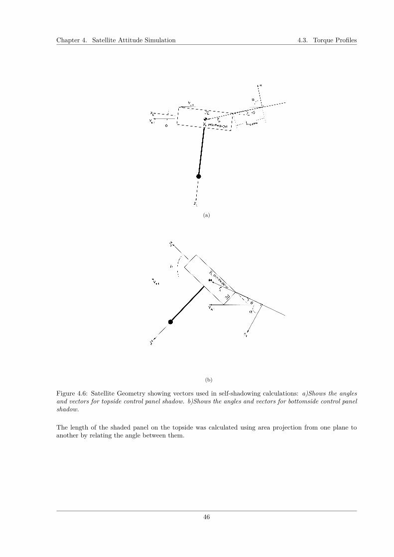
Chapter 4. Satellite Attitude Simulation 4.3. Torque Profiles
(a)
(b)
Figure 4.6: Satellite Geometry showing vectors used in self-shadowing calculations: a)Shows the anglesand vectors for topside control panel shadow. b)Shows the angles and vectors for bottomside control panelshadow.
The length of the shaded panel on the topside was calculated using area projection from one plane toanother by relating the angle between them.
46

Chapter 4. Satellite Attitude Simulation 4.3. Torque Profiles
Figure 4.7: Area projection. [10]
The new area, A′ is calculated by,
A′ = Acosθ (4.26)
Similarly, by using the pitch angle and the angle between the velocity vector and the normal vector of thepanel, as in figure 4.6, the shadowed area of the panel by the satellite bus can be calculated. Therefore,since the width of the panel and satellite bus are the same, the shaded lengths are calculated by,
Lshadowed,f = 2Lsin(α)cos(φ) (4.27)
Lshadowed,r = 2Lsin(β)cos(φ) (4.28)
where β = 90 − α, Lshadow,f is the length of the shaded top side and Lshadow,r is the length of theshaded bottom side of the panel.
In the algorithm for calculating the shaded length of the panel, Lshadow,f and Lshadow,r, are both setequal to zero when φ ≤ 0. In addition, for conditions when φ > 0, the shaded top side of the panelLshadow,f is set to zero if the shaded length is greater than the length of the panel (Lshadow,f > Lpanel).Similarly, the shaded bottom side of the panel Lshadow,r is set to zero if the shaded length is greaterthan the length of the panel (Lshadow,f > Lpanel). Otherwise in other conditions the shaded length inequations (4.27) and (4.28) are used to calculate the radius from the center of the shaded length to thecenter of gravity of the satellite. The calculation of the the radius of the shadowed panel is shown intable 4.4.
Side rp,xbrp,yb
rp,zb
rshadowed,f (Top Side) -Lshadowed,f
2 cos θ 0 Lshadowed,f
2 sin θrshadowed,r (Bottom Side) -Lshadowed,r
2 cos θ 0 Lshadowed,r
2 sin θ
Table 4.4: Location of the radius of the shaded panel length.
rp,f = rshadowed,f −CGposition (4.29)
rp,r = rshadowed,r −CGposition (4.30)
Once the radius rp from the shaded region of the panel to the center of gravity are known, the forces andmoments are then calculated using the same method as in section 4.2.2. Furthermore, to calculate theactual force and moment acting on the panel,
Factual = Funshadowed − Fshadowed (4.31)
Mactual = Munshadowed −Mshadowed (4.32)
47
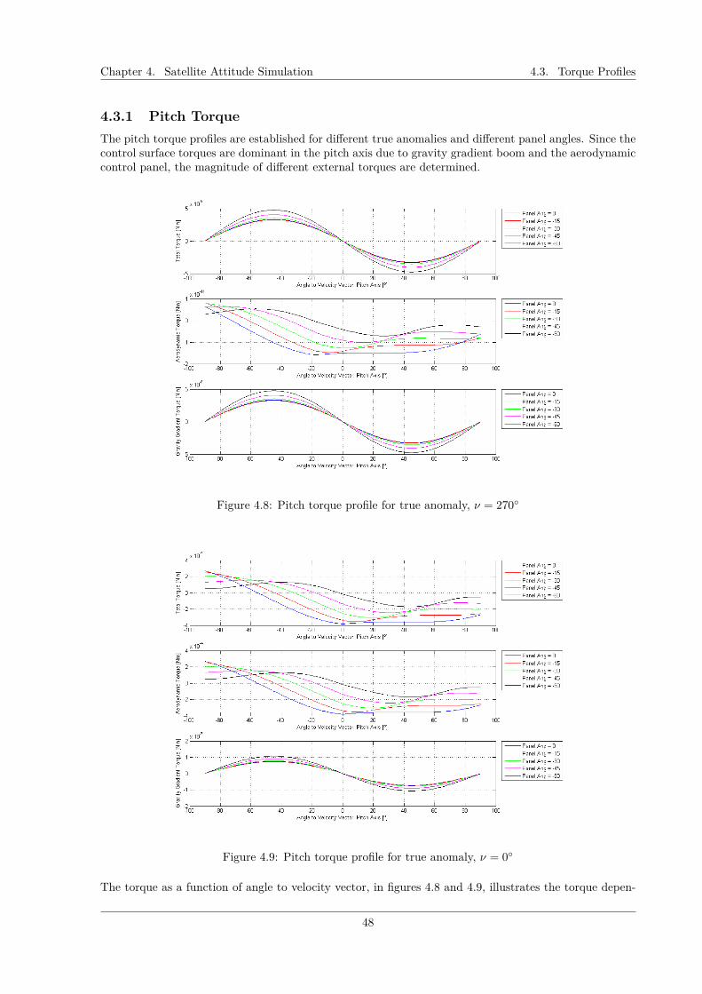
Chapter 4. Satellite Attitude Simulation 4.3. Torque Profiles
4.3.1 Pitch TorqueThe pitch torque profiles are established for different true anomalies and different panel angles. Since thecontrol surface torques are dominant in the pitch axis due to gravity gradient boom and the aerodynamiccontrol panel, the magnitude of different external torques are determined.
Figure 4.8: Pitch torque profile for true anomaly, ν = 270
Figure 4.9: Pitch torque profile for true anomaly, ν = 0
The torque as a function of angle to velocity vector, in figures 4.8 and 4.9, illustrates the torque depen-
48

Chapter 4. Satellite Attitude Simulation 4.3. Torque Profiles
dency to the pitch angle. When the control panel is shadowed, the torque curve is determined by thegravity gradient boom. However, at true anomaly of ν = 270, the gravity gradient torque is dominantdue to the low atmospheric density. On the contrary, at true anomaly, ν = 0, the aerodynamic torquesdominate. The equilibria are determined by zero crossing of the torque curve. The characterization ofthe zero crossing of the torque curve depends on which external torques are dominant. At the perigeepassage (ν = 0), the zero crossing of the torque curve is characterized by the aerodynamic torque due tohigher atmosphere density. At ν = 270, gravity gradient torque characterizes the torque curve due tolower atmospheric density.
Figure 4.10: Pitch torque of separate components, for true anomaly, ν = 270
49

Chapter 4. Satellite Attitude Simulation 4.3. Torque Profiles
Figure 4.11: Pitch torque of separate components, for true anomaly, ν = 0
Figures 4.10 and 4.11, show the aerodynamic torque profiles for the satellite bus, boom and control panel.The shadowing of the control panel can also be seen in both figures.
4.3.2 Yaw and Roll Torque Profiles
Figure 4.12: Yaw torque profile.
50

Chapter 4. Satellite Attitude Simulation 4.3. Torque Profiles
Figure 4.13: Roll torque profile
The yaw torque profile plotted in figure 4.12 is dominated by the aerodynamic torque. Since gravitygradient torque does not function in the yaw axis, the aerodynamic panel characterizes the torque curve.The equilibria are determined to be at yaw angles, −90, 0, and 90 due to the zero torque. The rolltorque profile in figure 4.13 is dominated by the gravity gradient torque, since the gravity gradient torqueapplies only to the pitch and roll axes. Consequently, there is no panel aerodynamic torque in the rollaxis due to the assumption that the thickness of the panel is zero.
Figure 4.14: Yaw torque of separate components.
51

Chapter 4. Satellite Attitude Simulation 4.4. Pitch Dynamics
There are torque profiles on the satellite bus, in figure 4.14, due to the center of mass shifting as the panelangle changes. It is interesting that the yaw torque has the same magnitude as the pitch torque. Forinstance the maximum pitch torque is 4×10⁻⁴ and the maximum yaw torque is 0.5×10⁻⁴, this could bedue to the fact that the Euler equations of motion are coupled. Hence, the pitch torque also contributesto the yaw torque. Additionally, there are no yaw torque profiles for the boom because here the boom isassumed to always be aligned with the center of mass.
4.4 Pitch DynamicsTo find a suitable attitude upon the satellite’s entrance into the perigee passage, the attitude dynamicsare investigated. The previous section explored the torque profiles of the satellite. From the torqueprofiles, the equilibria are determined by the zero crossing of the curve. Hence in this section multiplesimulations are done with different panel angles θ, angular rates ω, and attitude angles φ, in order to findthe combination that keeps the satellite’s attitude stable.
4.4.1 Initial Orbit Conditions for Pitch DynamicsThe initial orbit simulation conditions are presented in table 4.5. These values are decided based ondecay simulation results in section 3.2.4, where it was decided that an orbit with perigee of 168 km wasappropriate for the insertion orbit. The true anomaly is set at ν = 270, to indicate the perigee entranceof the satellite. The run time of the simulation is t = 2800 s, which is approximately where the satelliteexits the perigee passage.
Apogee a = 6000 kmPerigee p = 168 kmInclination i = 90True anomaly θ = 270Right ascension of the ascending node Ω = 0 Argument of perigee ω = 0 Eccentricity e = 0.3082Orbital period T = 9160 sMean motion n = 6.86×10⁻⁴
Table 4.5: Initial orbit simulation conditions.
4.4.2 Simulation ResultsIn the previous section, torque profiles of panel angles at θ = −45 and θ = −60 had the equilibriacrossings between φ2 = 0 and φ2 = −20. In order to keep the satellite stable, it is good to keep theinitial angle deviation as close to φ2 = 0 as possible. The pitch behavior has been primarily investigateddue to the satellite having control surfaces in the pitch axis, where these values are presented in tables4.6 and 4.7.
ω0 [rad/s] θ [deg] Roll φ1 [deg] Pitch φ2 [deg] Yaw φ3 [deg](0, -n, 0) −45 0 −10 0
(0, -1.5n, 0) −45 0 −10 0(0, -2n, 0) −45 0 −10 0
Table 4.6: Initial conditions for pitch dynamics for different angular velocities with a panel angle, θ =−45.
52

Chapter 4. Satellite Attitude Simulation 4.4. Pitch Dynamics
Figure 4.15: Euler angles φi for different ωi,t=t0 , and panel angle of θ = −45.
The simulation results in figure 4.15, have shown that the satellite appears to be stabilized throughout theperigee passage, with a pitch angle φ2 = −10, angular rate ω0 = (0,−2n, 0), and panel angle θ = −45.In addition, some yaw and roll coupling can be seen, however the magnitude is very small and can beignored.
ω0 [rad/s] θ [deg] Roll φ1 [deg] Pitch φ2 [deg] Yaw φ3 [deg](0, -n, 0) −60 0 −3 0
(0, -1.5n, 0) −60 0 −3 0(0, -1.78n, 0) −60 0 −3 0
Table 4.7: Initial conditions for pitch dynamics for different angular velocities with a panel angle, θ =−60.
Figure 4.16: Euler angles φi for different ωi,t=t0 , and panel angle of θ = −60.
The simulation results in figure 4.15, have shown that the satellite appears to be stabilized throughoutthe perigee passage, with a pitch angle φ2 = −3, angular rate ω0 = (0,−1.78n, 0), and panel angleθ = −60. There is also some yaw and roll coupling that occurred, but again the magnitude is very smalland it can be ignored.
The two results demonstrated that the satellite can be stabilized in the perigee passage by with thecombination of aerodynamic drag panel and gravity gradient boom. The satellite with a deployable con-trol panel angle of θ = −45 is stable when entering at a pitch angle of φ2 = −10 and an initial angularvelocity of ω2,t=t0 = −2n [rad/s]. Similarly, the deployable control panel angle of θ = −60 is stablewhen entering at a pitch angle of φ2 = −3 and an initial angular velocity of ω2,t=t0 = −1.78n [rad/s].Additionally, it is good to note that although the yaw and roll coupling is minor, the oscillations seemto increase with time. Therefore, the yaw and roll oscillations could render the satellite unstable aftermany orbits, if it is not corrected.
53

Chapter 4. Satellite Attitude Simulation 4.5. Summary
4.5 SummaryIn this section, the torque profiles were established to better understand the behavior of the satelliteduring the perigee passage. The torque profiles done with multiple panel angles yielded equilibria zerocrossings, where it could be possible to stabilize the satellite. The panel angles that provided the zerocrossing of the torque with minimum deviation from the zero pitch angle were θ = −45 and −60. Thensimulations were done to investigate the attitude and angular rate of the satellite during the perigeepassage. It was found that at control panel angle of θ = −45, the satellite was stable given the initialconditions of pitch angle and angular rate to be, φ2 = −10 and ω2,t=t0 = −2n [rad/s]. Similarly, thecontrol panel angle of θ = −60 was stable given the initial conditions of pitch angle and angular rate tobe, φ2 = −3 and ω2,t=t0 = −1.78 [rad/s].
54
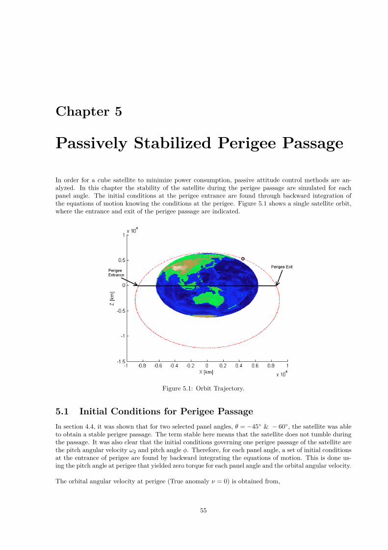
Chapter 5
Passively Stabilized Perigee Passage
In order for a cube satellite to minimize power consumption, passive attitude control methods are an-alyzed. In this chapter the stability of the satellite during the perigee passage are simulated for eachpanel angle. The initial conditions at the perigee entrance are found through backward integration ofthe equations of motion knowing the conditions at the perigee. Figure 5.1 shows a single satellite orbit,where the entrance and exit of the perigee passage are indicated.
Figure 5.1: Orbit Trajectory.
5.1 Initial Conditions for Perigee PassageIn section 4.4, it was shown that for two selected panel angles, θ = −45 & − 60, the satellite was ableto obtain a stable perigee passage. The term stable here means that the satellite does not tumble duringthe passage. It was also clear that the initial conditions governing one perigee passage of the satellite arethe pitch angular velocity ω2 and pitch angle φ. Therefore, for each panel angle, a set of initial conditionsat the entrance of perigee are found by backward integrating the equations of motion. This is done us-ing the pitch angle at perigee that yielded zero torque for each panel angle and the orbital angular velocity.
The orbital angular velocity at perigee (True anomaly ν = 0) is obtained from,
55

Chapter 5. Passively Stabilized Perigee Passage 5.2. Simulation Results
ω2,ν=0 = r × v|r|2
(5.1)
where r is the radius and v is the orbital velocity. The radius and velocity values used to calculateequation (5.1) are presented in table 5.1.
Variables x y zRadius, r [km] 6552.089 0 -2377.168Velocity, v [km/s] 0.2571354 0 8.917172
Table 5.1: Orbit radius and velocity at perigee.
Table 5.2, shows the pitch angle that yields zero torque at the perigee for different panel angles. Theseconditions are used for backward integration of equations of motion during the perigee passage, in orderto get the initial condition at the entrance of the perigee trajectory.
Torques [N·m] Panel Angle θ [] Zero-torque Pitch Angle φ2,ν=0 []0 0 -550 -15 -440 -30 -320 -45 -180 -60 -3
Table 5.2: Orbit radius and velocity at perigee.
5.2 Simulation Results
Panel Angle θ [] Initial Pitch Angle φν=270 [] Pitch Angular Velocity ω2,ν=270 [rad/s]-60 -4.332 -0.0012622-45 -13.68 -0.0014083-30 -24.39 -0.0014728-15 -30.64 -0.00153260 -36.88 -0.0015925
Table 5.3: Initial condition for different panel angles.
Figure 5.2: Attitude angles for different panel angle.
56

Chapter 5. Passively Stabilized Perigee Passage 5.3. Summary
The initial conditions at the entrance of the perigee passage are shown in table 5.3, where it ensures thatthe satellite does not tumble. For each panel angle, there is a corresponding initial pitch angle φν=270and a pitch angular velocity ω2,ν=270. In figure 5.2 it is seen that for all panel angles simulated there aresome disturbances at the perigee, this could be due to the same orbital angular velocity ω2,ν=0 used tobackward integrate the initial conditions.
5.3 SummaryThis section investigates the initial conditions for each panel setting to be able to remain stable throughthe perigee passage. A stable pitch attitude depends on the on the initial pitch angular velocity andpitch angle, where they were obtain by backward integrating the pitch angular velocity and pitch angleconditions at the perigee. The the initial pitch angular velocity and pitch angle that yields a stableperigee passage were found by using this method.
57

Chapter 6
Satellite Formation Design
In order to make multiple in situ measurements of the Aurora, a formation of satellites need to beexamined. As the satellite industry realizes the potential of cost reduction replacing conventional satelliteswith a multiple Cube Satellite formation, formation flying has become an increasingly popular subjectof study. There are a few different types of satellite formations, such as orbit tracking, leader-follower,virtual structure and swarming. The type of formation flying that is investigated in this thesis, is theleader-follower satellite formation in order to simplify the simulation to two satellites. This chapterincludes the definitions of coordinate reference frames and coordinate frame transformations used in themodeling of the leader-follower formation. A derivation of elliptic Earth orbits of the relative translationbetween the leader and follower satellite formation is shown [23].
6.1 Coordinate FrameThe Earth-Centered-Inertia (ECI) coordinate reference frame described in section 2.2.1 is reiterated hereto help clarify the satellite formation reference frames. In addition, the leader orbit reference frame andfollower orbit reference frame are also defined.
Earth-Centered-Inertia (ECI), is denoted as frame, i = (ix, iy, iz), has the vector ix pointing tothe vernal equinox, the iz vector points out of the Earth’s north pole, and the iy vector is orthogonal tothe other two vectors, and the location of its origin is at the center of the Earth.
Leader orbit reference frame is denoted as Fl, where its origin is at the center of mass of theleader satellite.
58

Chapter 6. Satellite Formation Design 6.2. Formation Dynamics
Figure 6.1: Reference coordinate frames. [11]
The er axis in the frame is parallel to the rl which points from the center of the Earth to the satellite.The eh axis is parallel to the orbit momentum vector, where it points in the orbit normal direction.Lastly, the eθ axis completes the right-handed orthogonal frame. These basis vectors are defined as,
er = rlrl
eθ = eh × er
eh = h
h
(6.1)
where h = rl × rl is the angular momentum vector of the orbit and h = |h|.
Follower orbital frame is denoted as Ff , where it has its origin at the center of mass of the fol-lower satellite. The vector rf is the vector pointing from the center of the Earth to the center of thefollower orbit frame. In figure 6.1, the origin of the follower orbit reference frame, expressed in Ff islocated by a relative orbit position vector p = [x y z]T . The frame unit vectors align with the basisvector Fl. The relative orbit position vector is defined as,
p = rf − rl = xer + yeθ + zeh (6.2)
Body reference frame is previously defined in section 2.2.1. The body frames in this section aredenoted as Fl and Ff , which the subscript l is the body reference frame of the leader satellite. Similarlythe subscript f denotes the follower body reference frame.
6.2 Formation DynamicsThe general equation of relative motion of two bodies, equation (2.6) from section 2.1.1, is adapted toexpress the dynamics of the leader and follower satellite as,
rl = − µr3l
rl + fdlmlrf = − µ
r3f
rf + fdfmf
(6.3)
where fdl and fdf are the orbital perturbations terms. Then the second order derivative of the relativeposition is expressed as,
59

Chapter 6. Satellite Formation Design 6.2. Formation Dynamics
p = rf − rl
= − µ
r3f
rf + fdfmf
+ µ
r3l
rl −fdlml
(6.4)
then it is rewritten as,
mf p = −mfµ
(rl + p
(rl + p)3 −rlrl
)+(fdf −
mf
mlfdl
)(6.5)
From equation (6.2), the dynamics of the follower satellite relative to the leader satellite is expressed inthe orbit frame Fl as,
rf = rl + p= (rl + x) er + yeθ + zeh
(6.6)
then differentiating twice with respect to time gives,
rf = (rl + x) er + 2 (rl + x) er + (rl + x) er + yeθ + 2yeθ + yeθ + zeh + 2zeh + zeh (6.7)
Furthermore, using true anomaly ν for the leader satellite the relationship between the true anomaly andthe follower orbit reference frame as [23],
er = νeθ (6.8)
eθ = −νer (6.9)
er = νeθ − ν2er (6.10)
eθ = −νer − ν2eθ (6.11)
The ideal case of the satellite is when there are no out of plane motion, therefore, eh = e = 0. Theninserting equations (6.8)-(6.11) into equation (6.7) yields,
rf =(rl + x− 2yν − ν2 (rl + x)− yν
)er +
(y + 2ν (rl + x) + ν (rl + x)− yν2) eθ + zeh (6.12)
Additionally, the position of the leader satellite is expressed as rl = rler where it is differentiate twicewith respect to time and inserting to equations (6.8)-(6.11) to become,
rl = rler + 2rler + rler
=(rl − rlν2) er + (2rlν + rlν) eθ
(6.13)
By taking the difference between equation (6.12) and (6.13), the result is the acceleration vector in theFl reference frame as,
p = rf + rl=(x− 2νy − ν2x− νy
)er +
(y + 2νx+ νx− ν2y
)eθ + zeh
(6.14)
Substituting (6.14) into (6.5) and setting v = p, produces the nonlinear relative equations of motion inthe form,
p = v (6.15)
60
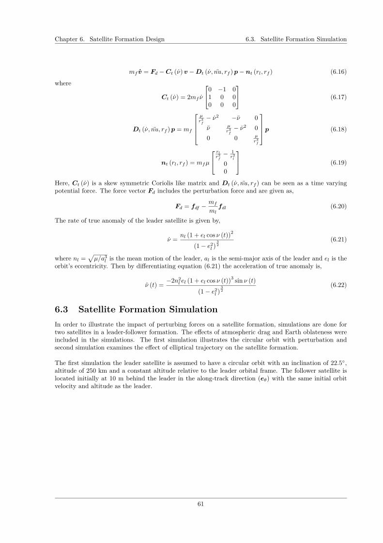
Chapter 6. Satellite Formation Design 6.3. Satellite Formation Simulation
mf v = Fd −Ct (ν)v −Dt (ν, nu, rf )p− nt (rl, rf ) (6.16)
where
Ct (ν) = 2mf ν
0 −1 01 0 00 0 0
(6.17)
Dt (ν, nu, rf )p = mf
µr3
f
− ν2 −ν 0ν µ
r3f
− ν2 00 0 µ
r3f
p (6.18)
nt (rl, rf ) = mfµ
rl
r3f
− 1r2
l
00
(6.19)
Here, Ct (ν) is a skew symmetric Coriolis like matrix and Dt (ν, nu, rf ) can be seen as a time varyingpotential force. The force vector Fd includes the perturbation force and are given as,
Fd = fdf −mf
mlfdl (6.20)
The rate of true anomaly of the leader satellite is given by,
ν = nl (1 + el cos ν (t))2
(1− e2l )
32
(6.21)
where nl =õ/a3
l is the mean motion of the leader, al is the semi-major axis of the leader and el is theorbit’s eccentricity. Then by differentiating equation (6.21) the acceleration of true anomaly is,
ν (t) = −2n2l el (1 + el cos ν (t))3 sin ν (t)
(1− e2l )
32
(6.22)
6.3 Satellite Formation SimulationIn order to illustrate the impact of perturbing forces on a satellite formation, simulations are done fortwo satellites in a leader-follower formation. The effects of atmospheric drag and Earth oblateness wereincluded in the simulations. The first simulation illustrates the circular orbit with perturbation andsecond simulation examines the effect of elliptical trajectory on the satellite formation.
The first simulation the leader satellite is assumed to have a circular orbit with an inclination of 22.5,altitude of 250 km and a constant altitude relative to the leader orbital frame. The follower satellite islocated initially at 10 m behind the leader in the along-track direction (eθ) with the same initial orbitvelocity and altitude as the leader.
61

Chapter 6. Satellite Formation Design 6.3. Satellite Formation Simulation
Figure 6.2: Relative position and velocity, in a circular orbit.
Figure 6.2 shows the relative position and velocity between two satellites in formation for a circular orbit.If there were no perturbations the relative translation would be constant. Hence it is seen in the figurethat the perturbation forces cause rather large oscillations in the relative translation. The Earth oblate-ness causes the follower satellite to experience the variation in gravity field, where as the leader satelliteonly experiences the ideal gravity force as if the Earth was a single point. The result is a stable cyclicoscillations in the radial direction (er). Similar oscillations are also seen in the cross-track direction (eh),which are due to the same variation in the gravity field that causes the oscillations in the radial directions.Since Earth is not a point mass, the follower satellite is then drawn towards the side with the largestgravitational pull. It also seems that the cross-track motion is less stable than the radial motion. As forthe along-track distance (eθ) between the leader and follower satellites, is not only oscillating but also de-caying. This behavior is due to the contribution of the atmospheric drag that are affecting both satellites.
The second simulation the leader satellite is assumed to have an elliptical orbit with an inclinationof 90, an apogee altitude of 6000 km and perigee altitude of 168 km. The follower satellite is initiallylocated 10 m behind the leader in the along-track direction (eθ) as well.
62
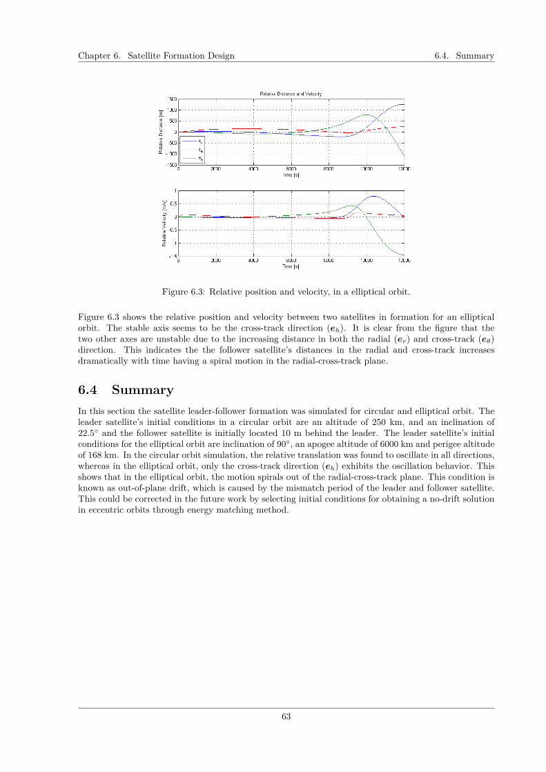
Chapter 6. Satellite Formation Design 6.4. Summary
Figure 6.3: Relative position and velocity, in a elliptical orbit.
Figure 6.3 shows the relative position and velocity between two satellites in formation for an ellipticalorbit. The stable axis seems to be the cross-track direction (eh). It is clear from the figure that thetwo other axes are unstable due to the increasing distance in both the radial (er) and cross-track (eθ)direction. This indicates the the follower satellite’s distances in the radial and cross-track increasesdramatically with time having a spiral motion in the radial-cross-track plane.
6.4 SummaryIn this section the satellite leader-follower formation was simulated for circular and elliptical orbit. Theleader satellite’s initial conditions in a circular orbit are an altitude of 250 km, and an inclination of22.5 and the follower satellite is initially located 10 m behind the leader. The leader satellite’s initialconditions for the elliptical orbit are inclination of 90, an apogee altitude of 6000 km and perigee altitudeof 168 km. In the circular orbit simulation, the relative translation was found to oscillate in all directions,whereas in the elliptical orbit, only the cross-track direction (eh) exhibits the oscillation behavior. Thisshows that in the elliptical orbit, the motion spirals out of the radial-cross-track plane. This condition isknown as out-of-plane drift, which is caused by the mismatch period of the leader and follower satellite.This could be corrected in the future work by selecting initial conditions for obtaining a no-drift solutionin eccentric orbits through energy matching method.
63

Chapter 7
Conclusion
The CubeSat configuration has been proven to reduce cost and development time. This has enabled anaffordable way for universities to perform experiments and test instruments in space. The Space andPlasma Physics department at Kungliga Tekniska Hogskolan has proposed a scientific mission to studythe aurora in response to the Swedish National Space Board’s appeal for ideas of innovative low-cost sci-entific satellite missions. The mission requires a closely spaced 3-U CubeSat formation in order to makemultiple in situ measurements of the aurora. The apogee and perigee of the mission are 6000 km and200 km. In addition, the thesis also explores the use of passive control methods for orbit and formationcontrol. This was done through gravity gradient and aerodynamic torques. The thesis is a preliminarymission analysis and design of a small satellite swarm. Further expansion of previous simulation codedeveloped for the SWIM project was done in the program MATLAB.
In the nature of a highly eccentric orbit, a more accurate atmospheric model was needed to approxi-mate orbital decay. The NRLMSISE-00 atmospheric model was chosen not only because of the extensivesatellite drag data and accelerometer data on the total mass density, but also the greater detail of thedensity variations. From the results of the orbital decay simulation, the insertion orbit was found to beat a perigee of 168 km and an apogee of 6000 km, where it was possible for the satellite with a ram-facingarea of atleast 0.1 m2 to decay in 90 days.
The satellite’s combination of gravity gradient and aerodynamic torques were analyzed to establish thebehavior of the satellite during the perigee passage. The satellite was configured with a gravity gradientboom and an aerodynamic drag panel. The pitch torque profiles were found for multiple panel anglesthat supplied zero-torque. The panel angles -45 and -60 were then simulated to establish the initialconditions of pitch angle and angular rate at the entrance of the perigee passage that returned a non-tumbling trajectory. Furthermore, a method was developed to find initial conditions for all panel anglesby utilizing pitch angle that yielded zero-torque at the perigee. Knowing this the initial conditions for allpanel angles that returned a non-tumbling perigee trajectory were found by backwards integration of thepitch angle and angular rate conditions at perigee. The simulations indicate that for atleast one perigeepassage at a perigee altitude of 168 km, the satellite was able to maintain its attitude and not tumble.
Since a swarm of satellites would eventually be used to make an in situ observation, a brief simula-tion of a satellite formation was done on a leader-follower configuration. A circular and elliptical orbitsof the relative translation were simulated. It was found that the relative translation of a circular orbitoscillates in all relative directions, whereas in an elliptical orbit it only oscillates in the cross-track direc-tion. In addition, the simulation has shown that a leader-follower formation with a elliptical referenceorbit, the relative translation would spiral out of the radial-cross-track plane.
The preliminary study done in this thesis have found that a satellite with a constant ram-faced areaof 0.1 m2 would be able to achieve an orbit decay of 90 days. However, further investigations are neededto establish a more linear orbit decay. Although a stable pitch attitudes with the combination of gravitygradient and aerodynamic drag panel were found, they were only simulated for a single perigee passage
64

Chapter 7. Conclusion
and perigee altitude. Further analyses are needed in order to obtain other initial conditions at the entranceof the perigee passage, which would ensure a non-tumbling passage as the satellite decays. Additionally,further studies are needed to examine if the satellite yaw axis can be controlled, by adding additionalpanels on the side. Lastly, simulations of the leader-follower satellite yielded an out of plane behaviorfor an elliptical orbit. This could be corrected in future works by determining the initial conditions thatmatches the period of the leader and follower satellite.
65

Bibliography
[1] Pumpkin Inc., “http://www.cubesatkit.com/content/design.html,” June 2012.
[2] J. Wertz and L. Wiley, Space Mission Analysis and Design. Space Tehnology Library, third ed.,2008.
[3] H. D. Curtis, Orbital mechanics for engineering students [Elektronisk resurs]. Elsevier LTD., 2005.
[4] R. R. Bate, D. D. Mueller, and J. E. White, Fundamentals of Astrodynamics. Dover Publications,Inc., 1st ed., 1971.
[5] B. Wie, Space Vehicle Dynamics and Control. AIAA Education Series, 2nd ed., 2008.
[6] V. A. Chobotov, Orbital Mechanics. AIAA Education Series, AIAA Education Series, 1991.
[7] M. Griffin and J. French, Space Vehicle Design. AIAA Education Series, second ed., 2004.
[8] W. Wiesel, Spaceflight Dynamics. Irwin McGraw-Hill, second ed., 1997.
[9] M. L. Gargasz, “Optimal spacecraft attitude control using aerodynamic torques,” thesis, Air ForceInstitute of Technology, Wright-Patterson Air Force Base, Ohio, March 2007.
[10] L. Rade and B. Westergren, Mathematics Handbook for Science and Engineering. Studentlitteratur,2004.
[11] H. Schaub and J. L. Junkins, Analytical Mechanics of Space Systems. AIAA Education Series, 2003.
[12] J. Zorita, “Dynamics of small satellites with gravity gradient attitude control,” master thesis, Kung-liga Tekniska Hogskolan, Electrical Engineering Department, KTH Kungliga Tekniska Hogskolan,SE-100 44 Stockholm Sweden, October 2011.
[13] R. Battin, An Introduction to the Mathematics and Methods of Astrodynamics. AIAA EducationSeries, 1987.
[14] “Guid to reference and standard atmosphere models,” Tech. Rep. G-003B2-2004, American NationalStandards Institute, 2004.
[15] G. Y. Lou, “Models of earth’s atmosphere (90 to 2500 km),” Space Vechicle Design Criteria SP-0021,NASA, 1973.
[16] G. P. Newton and D. T. Pelz, “Latitudinal variations in the neutral atmospheric density,” J. Geophys.Res., vol. 74, no. 16, pp. 4169–4174, 1969.
[17] The MathWorks, Inc., MATLAB Mathematics.
[18] J. M. Picone, A. E. Hedin, and D. P. Drob, “Nrlmsise-00 empirical model of the atmosphere: Statis-tical comparisons and scientific issues,” Journal of Geophysical Research, vol. 107, no. A12, p. 1468,2002.
[19] G. Cook, “Satellite drag coefficients,” Planetary and Space Science, vol. 13, no. 10, pp. 929 – 946,1965.
66

Bibliography Bibliography
[20] K. Moe and M. M. Moe, “Gas–surface interactions and satellite drag coefficients,” Planetary andSpace Science, vol. 53, no. 8, pp. 793 – 801, 2005.
[21] M. L. Psiaki, “Nanosatellite attitude stabilization using passive aerodynamics and active magnetictorquing,” Journal of Guidance, Control and Dynamics, vol. 27, pp. 347–355, May-June 2004.
[22] P. C. Hughes, Spacecraft Attitude Dynamics. Dover Books, 2004.
[23] R. Kristiansen, Dynamic Synchronization of Spacecraft. PhD thesis, Norwegian University of Scienceand Technology, 2008.
67