Southern Methodist University Southern Methodist University

SMU Scholar SMU Scholar

Civil and Environmental Engineering Theses and Dissertations

Civil Engineering and Environmental Engineering

Spring 5-16-2020

Space and Depth-Resolved Naturally Occurring Toxic Groundwater Space and Depth-Resolved Naturally Occurring Toxic Groundwater

Species in Bangladesh and Rwanda: Origination and Risk Analysis Species in Bangladesh and Rwanda: Origination and Risk Analysis

Kenneth Hamilton khamilton@smu.edu

Follow this and additional works at: https://scholar.smu.edu/engineering_civil_etds

Part of the Environmental Engineering Commons, Environmental Indicators and Impact Assessment

Commons, Environmental Monitoring Commons, and the Geochemistry Commons

Recommended Citation Recommended Citation Hamilton, Kenneth, "Space and Depth-Resolved Naturally Occurring Toxic Groundwater Species in Bangladesh and Rwanda: Origination and Risk Analysis" (2020). Civil and Environmental Engineering Theses and Dissertations. 7. https://scholar.smu.edu/engineering_civil_etds/7

This Dissertation is brought to you for free and open access by the Civil Engineering and Environmental Engineering at SMU Scholar. It has been accepted for inclusion in Civil and Environmental Engineering Theses and Dissertations by an authorized administrator of SMU Scholar. For more information, please visit http://digitalrepository.smu.edu.

Space and Depth-Resolved Naturally Occurring Toxic Groundwater Species in Bangladesh and

Rwanda: Origination and Risk Analysis

Approved by:

_______________________________________

Prof. Andrew Quicksall

Associate Professor of Civil & Environmental

Engineering

___________________________________

Prof. John Easton

Senior Lecturer of Civil & Environmental

Engineering

___________________________________

Prof. Jaewook Myung

Assistant Professor of Civil & Environmental

Engineering

___________________________________

Prof. Wenjie Sun

Assistant Professor of Civil & Environmental

Engineering

___________________________________

Dean James Quick

Associate Vice President for Research

Dean of Graduate Studies

Professor of Earth Sciences

Space and Depth-Resolved Naturally Occurring Toxic Groundwater Species in Bangladesh and

Rwanda: Origination and Risk Analysis

A Dissertation Presented to the Graduate Faculty of

Lyle School of Engineering

Southern Methodist University

in

Partial Fulfillment of the Requirements

for the degree of

Doctor of Philosophy

with a

Major in Civil & Environmental Engineering

by

Kenneth M. Hamilton II

(B.S., Environmental Engineering, Southern Methodist University)

(M.S., Environmental Engineering, Southern Methodist University)

May 16, 2020

Copyright (2019)

Kenneth M. Hamilton II

All Rights Reserved

iv

ACKNOWLEDGMENTS

This work could not have been accomplished by the wisdom of my brilliant advisor, Dr.

Andrew Quicksall, along with his many colleagues in the Department of Civil and

Environmental Engineering here at SMU. I'm also forever grateful for everyone involved in this

process. Expressly my Mum and Dad for remaining patient with me through this long intellectual

development. My friends, for always making sure I knew good times were ahead, Mrs. Salcedo

for making sure I was fed, Mr. Salcedo for the Sunday soccer lessons and, Monica for always

cheering me on.

v

Hamilton, Kenneth B.S., Environmental Engineering, Southern Methodist University, 2012

M.S., Environmental Engineering, Southern Methodist University, 2013

Space and Depth-Resolved Naturally Occurring Toxic

Groundwater Species in Bangladesh and Rwanda:

Origination and Risk Analysis

Advisor: Andrew N. Quicksall

Doctor of Philosophy conferred May 16, 2020

Dissertation completed April 17, 2020

Access to safe potable water is a necessity for all. Groundwater is a commonly

relied upon drinking water source for many areas around the world. This is especially true for

communities in high density, rural settings. Such is the case for populations near Cox’s Bazaar,

Bangladesh, and in the Bugesera region of Rwanda. Sediment and groundwater contamination,

through toxic dissolved species, represents a significant public health risk to exposed

populations. Tropical soils, such as the soil profiles in Bangladesh and Rwanda, often contain

higher concentrations of heavy metals (Rieuwerts, 2007). Additionally, nitrate from fertilizers,

are widely used on the soils in these regions. While hazardous risk will never be alleviated in its

entirety, it is the goal to diminish the threat as much as possible. To accomplish this task, a

complete and fundamental understanding of contaminant solid-solution partitioning mechanisms

is required. It is also important to note that contaminant distribution over space and depth is a

contributing factor to potential exposure. The outcome of this dissertation combines spatial- and

depth-resolved sampling to quantify contamination risk posed by heavy metals and other toxic

vi

species. In finding and evaluating these hazardous risks, potential solutions to alleviate and

manage public health exposure are offered.

The first chapter involved groundwater sampling at Kutupalong settlement camp near

Cox’s Bazaar, Bangladesh. Sponsored by the United Nations High Commissioner for Refugees

(UNHCR), thorough sampling of the community’s potable groundwater, took place throughout

the entire settlement. Sampling uncovered subsurface biogeochemical processes that ultimately

govern the release of Pb and NO3-. Pb concentrations were found as elevated as 150µg/L, well

above the World Health Organization’s guideline of 10µg/L Pb in drinking water. Further

investigation indicated nitrogen dynamics regulate pH in the subsurface. Changes in pH control

the solubility of Fe and Mn oxides and, therefore, their associated sorption and desorption of Pb.

Contaminant release is spatially heterogeneous within the resettlement’s groundwater. This

would make in situ remediation a tedious and possibly ineffective solution. To compensate,

geochemical data in combination with GIS spatial analysis generated risk assessment maps. The

maps illustrate the heterogeneity of risk associated with distinct contaminants throughout

Kutupalong. In doing so, risk maps provide a mitigation strategy of avoidance for contaminated

well sites, strategic guidance for currently safe wells, the closure of high-risk wells, and the

placement of future ones.

The second study in this dissertation looked at naturally occurring metal contamination in

groundwater from a tropical region. Water quality mapping in Bugesera, Rwanda, highlighted

multiple metal contaminations throughout the region. Multiple in-use boreholes contained Mn

exceeding the former WHO guideline of 400µg/L. Several sites also contained U exceeding the

WHO guideline of 30µg/L. U was found to be over 50µg/L in some cases and over 400µg/L in

one extreme circumstance. Sediment sampling in 2016 and 2017 helped verify that multiple

vii

areas within Bugesera contain elevated solid-phase concentrations of various metals with very

different mechanisms of potential release into the environment. Three different sites were

sampled and assessed for concentrations of multiple heavy and trace metals. Among the metals

evaluated, Mn, U, and V presented the highest levels of sediment concentrations. Depth-

resolved sampling uncovered subsurface characteristics unique to each locale. Depth to

groundwater table and associated redox changes varied by locale. A location with seasonally

persistent vadose conditions is contrasted with locations showing redox changes induced by

seasonally fluctuation pore saturation via groundwater table oscillation.

Sequential extraction experiments were completed to identify the metal speciation. Loss

on ignition (LOI), calcination, and soil acidity measurements further characterize the sediment

chemical systems and provide depth to interpretation as to the mobility of the metals. This

research aims to characterize the elevated metal concentrations in the subsurface as well as

determine the mechanisms of release for potential exposure to the environment and the public

health. Ultimately, this will permit communities within Bugesera to develop without risk of

exposure to toxic metals.

The final phase of research looked beyond the soil-water interface and studies

contamination exposure through fine sediment particles. Small size airborne particles are well-

known pathways for chemical exposure, including exposure to heavy metals. Though metals

concentrations are important, they alone do not verify the complete exposure sediments or

sediment particles present. Hakanson (1980) and Tomlinson et al. (1980) describe ecological risk

indices that give a more accurate assessment of contamination risk. By using contamination

factors (Cf), pollution load index (PLI), and potential ecological risk index (RI), an accurate

assessment of the toxicity and exposure by fine sediment particles can be calculated. In this

viii

study, two different locations in Bugesera are examined. It is found that sub 75µm particles

present a far greater level of potential exposure risk than larger particle sizes. The greatest

potential hazard comes from a region with constant redox cycling. Metals of most concern, at

this location, are Cu and Pb. The other studied site is a region with a yearly constant vadose

zone. At this location most concerning metals are Pb, Cd, and Cu.

Through understanding the biogeochemical processes, their independent release

mechanisms, and potential exposure risk, informed, adequate, and necessary management

judgments can be determined. Whether decisions are made for strategic avoidance or direct

mitigation, responsible parties cannot do so without the pertinent information from in-depth

examination. The complete aim of this dissertation looks to gather all necessary information to

make sound decisions in keeping the public health at large protected from toxic metal exposure,

specifically metal exposure from tropical soils.

ix

TABLE OF CONTENTS

LIST OF FIGURES ................................................................................................................... xi

LIST OF TABLES ................................................................................................................... xiii

CHAPTER 1 .............................................................................................................................. 1

1.1 Background ....................................................................................................................... 1

1.2 Metals & Toxic Species .................................................................................................... 2

1.3 Distribution Mapping ........................................................................................................ 5

1.4 Ecological Risk Assessment ............................................................................................. 6

1.5 Research ............................................................................................................................ 6

1.6 Figures............................................................................................................................... 8

CHAPTER 2 ............................................................................................................................... 9

Abstract ................................................................................................................................... 9

2.1 Introduction ..................................................................................................................... 11

2.2 Methods........................................................................................................................... 14

2.3 Chemical Analysis and Correlation ................................................................................ 18

2.6 Figures and Tables .......................................................................................................... 25

CHAPTER 3 ............................................................................................................................. 35

Abstract ................................................................................................................................. 35

3.1 Introduction ..................................................................................................................... 37

x

3.2 Methods........................................................................................................................... 39

3.3 Results ............................................................................................................................. 43

3.4 Discussion ....................................................................................................................... 48

3.6 Conclusion ...................................................................................................................... 52

3.7 Figures and Tables .......................................................................................................... 54

CHAPTER 4 ............................................................................................................................. 78

Abstract ................................................................................................................................. 78

4.1 Introduction ..................................................................................................................... 79

4.2 Methods........................................................................................................................... 81

4.3 Results ............................................................................................................................. 88

4.4 Discussion ....................................................................................................................... 90

4.5 Conclusion ...................................................................................................................... 93

4.6 Figures & Tables ............................................................................................................. 95

CHAPTER 5 ........................................................................................................................... 107

5.1 Summarization .............................................................................................................. 107

Appendix A ............................................................................................................................. 112

BIBLIOGRAPHY ................................................................................................................... 132

xi

LIST OF FIGURES

Figure 1.1) Location of Kutupalong Resettlement Camp in Bangladesh. ...................................... 8

Figure 1. 2) Map of Rwanda and the Bugesera District ................................................................. 8

Figure 2. 1) Pb & NO3- concentration with pH ............................................................................. 25

Figure 2. 2) Mn & Fe concentrations with ORP ........................................................................... 26

Figure 2. 3) Mn & Fe concentrations with shifting pH................................................................. 27

Figure 2. 4) SO42- concentration with shifting pH ........................................................................ 28

Figure 2. 5) Interpolated Map of Mn ............................................................................................ 29

Figure 2. 6) Interpolated Map of Fe .............................................................................................. 30

Figure 2. 7) Interpolated Map of Pb.............................................................................................. 31

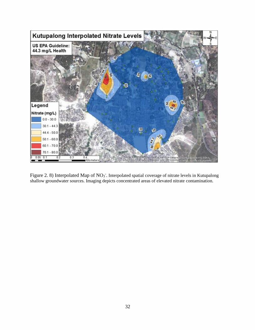
Figure 2. 8) Interpolated Map of NO3- .......................................................................................... 32

Figure 2. 9) Interpolated Map of pH ............................................................................................. 33

Figure 2. 10) Risk Map ................................................................................................................. 34

Figure 3. 1) SOM & Carbonate material at Site1 and Site2 ......................................................... 55

Figure 3. 2) Error of SOM and carbonate matter at Lowland Marsh ........................................... 56

Figure 3. 3) Error of SOM and Carbonate Material at Mining Hill .............................................. 57

Figure 3. 4) SOM & Carbonate Material at Site3 ......................................................................... 58

Figure 3. 5) Error on SOM and Carbonate Material at Agricultural Field ................................... 59

Figure 3. 6) Mn concentrations at Site1 ........................................................................................ 60

Figure 3. 7) Mn speciation at Site1 ............................................................................................... 61

Figure 3. 8) U concentrations at Site1 .......................................................................................... 62

Figure 3. 9) U speciation at Site1.................................................................................................. 63

Figure 3. 10) V concentrations at Site1 ........................................................................................ 64

xii

Figure 3. 11) V speciation at Site1................................................................................................ 65

Figure 3. 12) Manganese concentrations at Site2 ......................................................................... 66

Figure 3. 13) Mn speciation at Site2 ............................................................................................. 67

Figure 3. 14) U concentrations at Site2 ........................................................................................ 68

Figure 3. 15) U speciation at Site2................................................................................................ 69

Figure 3. 16) V concentrations at Site2. ....................................................................................... 70

Figure 3. 17) V speciation at Site2................................................................................................ 71

Figure 3. 18) Mn concentrations at Site3. ..................................................................................... 72

Figure 3. 19) Mn speciation at Site3 ............................................................................................. 73

Figure 3. 20) U concentrations at Site3 ........................................................................................ 74

Figure 3. 21) U speciation at Site3................................................................................................ 75

Figure 3. 22) V concentrations at Site3. ....................................................................................... 76

Figure 3. 23) V speciation at Site3................................................................................................ 77

Figure 4. 1) Site1 A’s Particle Size Distribution .......................................................................... 95

Figure 4. 2) Site1 B’s Particle Size Distribution........................................................................... 96

Figure 4. 3) Site2 A’s Particle Size Distribution .......................................................................... 97

Figure 4. 4)Site2 B’s Particle Size Distribution............................................................................ 98

Figure 4. 5) Soil Acidity for Sites1 & 2 ........................................................................................ 99

Figure 4. 6) The SOM and Carbonate Material .......................................................................... 102

Figure 4. 7) The average PLI per particle size for both Site1 and Site2 ..................................... 104

Figure 4. 8) The Risk Index of each particle size for Site1 and Site2 ........................................ 106

xiii

LIST OF TABLES

Table 3. 1) Location Soil Acidity ................................................................................................. 54

Table 4. 1) t-test results Comparing Average pH from Site1 and Site2 ..................................... 100

Table 4. 2) Average Concentrations ........................................................................................... 101

Table 4. 3) The average contamination factor ............................................................................ 103

Table 4. 4) Table of ER values .................................................................................................... 105

Appendix Table 1) ...................................................................................................................... 112

Appendix Table 2) ...................................................................................................................... 112

Appendix Table 3) ...................................................................................................................... 113

Appendix Table 4) ...................................................................................................................... 113

Appendix Table 5) ...................................................................................................................... 114

Appendix Table 6) ...................................................................................................................... 114

Appendix Table 7) ...................................................................................................................... 115

Appendix Table 8) ...................................................................................................................... 115

Appendix Table 9) ...................................................................................................................... 116

Appendix Table 10) .................................................................................................................... 117

Appendix Table 11) .................................................................................................................... 118

Appendix Table 12) .................................................................................................................... 118

Appendix Table 13) .................................................................................................................... 119

Appendix Table 14) .................................................................................................................... 119

Appendix Table 15) .................................................................................................................... 120

Appendix Table 16) .................................................................................................................... 120

Appendix Table 17) .................................................................................................................... 121

xiv

Appendix Table 18) .................................................................................................................... 121

Appendix Table 19) .................................................................................................................... 122

Appendix Table 20) .................................................................................................................... 122

Appendix Table 21) .................................................................................................................... 123

Appendix Table 23) .................................................................................................................... 125

Appendix Table 24) .................................................................................................................... 125

Appendix Table 25) .................................................................................................................... 126

Appendix Table 26) .................................................................................................................... 126

Appendix Table 27) .................................................................................................................... 127

Appendix Table 28) .................................................................................................................... 127

Appendix Table 29) .................................................................................................................... 128

Appendix Table 30) .................................................................................................................... 128

Appendix Table 31) .................................................................................................................... 129

Appendix Table 32) .................................................................................................................... 129

Appendix Table 33) .................................................................................................................... 130

1

CHAPTER 1

Introduction

1.1 Background

Soil-groundwater chemical interactions are part of a unique and complex relationship.

Understanding this association, its consequences on the environment, and its further impacts on

the human population, is imperative for public health and safety. Subsurface biogeochemical

reactions can result in the sequestration and/or release of toxic elements. Many trace and heavy

metals are concerning considering their inherent health risks posed to the public. While geogenic

toxic hydrated metal cations and oxyanions are hazardous worldwide, developing nations have a

particular vulnerability (Nriagu, 1992). Geopolitics and global economics are forces that bridge

public health to the environment. The work studied groundwater, sediments, and soil

groundwater interactions in susceptible areas of developing nations of interest. The Bugesera

district in Rwanda and a Rohingya refugee resettlement near Cox’s Bazaar, Bangladesh were

identified as areas of interest.

In 2011 and 2013, sampling trips to the Kutupalong settlement, was sponsored by the

United Nations High Commissioner for Refugees (UNHCR). Map 1 below, details the location

of Bangladesh and the Kutupalong settlement. It is a settlement for Rohingya refugees escaping

persecution in Myanmar. Kutupalong is located near the city of Cox’s Bazaar in Bangladesh's

2

hill tracts region. The shallow depth to bedrock hill tracts region in Bangladesh differs from the

more well known deep deltaic regions of the country associated with contamination of arsenic.

Geologically, the hill tracts have varied bedrock instead of the uniform Holocene sediment found

in the deltaic zone.

Rwanda is a small, inland, equatorial, east-central African nation and is geologically part

of the East African Rift Zone as shown in Map 2. The country is surrounded by the neighboring

rift valley nations Uganda, Democratic Republic of Congo, Tanzania, and Burundi. Rwanda

contains a variety of differing geologies and environmental systems. The Bugesera district in

Rwanda is a unique area directly south of the nation’s capital Kigali. The district is a drier region

than neighboring regions to the north and west yet it contains more surface water than the other

regions. Its geomorphology leads to numerous lakes and wetlands not seen elsewhere in the

region. Bugesera is the eastern province’s westernmost district. It borders the southern district to

the west, Kigali to the north, and Burundi to the south. Bugesera’s location is illustrated in Map

2.

1.2 Metals & Toxic Species

1.2.1 Heavy Metals

Uranium is a heavy metal, mostly associated with fuel for nuclear fission power

(Domingo, 2001; Winde et al., 2017). The public, therefore, commonly thinks of uranium risk as

its radioactivity. It is also, however, a highly toxic element when biologically absorbed in plants

and animals, including humans. Its absorption can lead to numerous toxicological human health

3

effects as well as deleterious effects on ecological systems (Selvakumar et al., 2018). In humans,

uranium accumulates most commonly in the liver, kidneys, and bones (Bajwa et al., 2017).

Uranium ingestion is mostly known as a nephrotoxin targeting proper kidney function (Kurttio et

al., 2005). Kurttio and others have studied natural uranium uptake, via drinking water, and its

affliction on human bone turnover (Kurttio et al., 2005). However, uranium is now also seen as

toxic to the human reproductive system (Shuang Wang et al., 2019). Naturally occurring uranium

is a toxic element and, therefore, of interest when it is found in aquifers and sediments. Uranium

is also frequently linked to other environmentally relevant geochemical cycles (Zavodska et al.,

2008).

Lead and manganese are both metals of environmental concern. In the case of lead, it is a

heavy metal with numerous health concerns (Flora et al., 2012; Roy and Edwards, 2019;

Trueman et al., 2019), including being expected as a human carcinogen (National Toxicology

Program, 2011; Rehman et al., 2018). Lead carcinogenicity is of immense concern due to

notable lead exposure globally (Silbergeld, 2003). Lead is widely documented as a neurotoxin,

contributing to neurophysiological damage and function decline (Mason et al., 2014). The

decline of nervous system functionality is associated with chronic exposure (Mason et al., 2014).

Experimental findings suggest lead’s neurological effects extend to intellectual deficiencies,

especially among children (Lanphear et al., 2005; Redmon et al., 2018; Slikker et al., 2018).

Manganese is a transition metal involved in environmentally important processes

(Herndon et al., 2018). It is essential for the proper biological function of living organisms

(Santamaria and Sulsky, 2010). It does not have the same health effects as many heavy metals,

but, at concentrations studied, is toxic with overexposure and can lead to numerous organ

failures (Crossgrove and Zheng, 2004). Manganese overexposure is correlated with decreased

4

fertility and other reproductive issues (Crossgrove and Zheng, 2004). In trace concentrations,

manganese is essential for brain development but overexposure will cause manganese to be a

toxicant to the brain (Takeda, 2003). In many instances, the exposure of either element is

governed by their geochemical intrarelationship in an environmental system (Dong et al., 2003,

O’Reilly and Hochella, 2003). The geochemistry of lead and manganese and their toxicological

impacts are described in more depth below.

1.2.2 Oxyanions

Oxyanions are anions attached to an oxygen atom and are similarly hydrated in solution.

Unlike hydrated cations, oxyanions can include metals, metalloids, and non-metals. Vanadium

and nitrate are typical examples of oxyanions.

Vanadium is a redox driven, transition metal, similar to chromium. Vanadium is a well

know geochemical constituent; however, studies into its environmental and health impacts have

lagged (Huang et al., 2015). There are numerous health effects associated with vanadium

(Guagliardi et al., 2018). Health implications due to vanadium exposure include poisoning of the

respiratory, circulatory, and nervous system as well as the kidneys and digestive organs

(Venkataraman and Sudha, 2005). Vanadium geochemistry is also an identifier for redox

changes (Huang et al., 2015). It has several oxidation states, but V(IV) & V(V) are the most

prevalent species in aqueous environments (Pourret et al., 2012). Understanding vanadium

speciation relationships will help yield a complete geochemical picture of the subsurface

environment.

Nitrogen dynamics strongly influence subsurface chemistry.

5

To fully comprehend certain geochemical trends, nitrate and other nitrogen species must be

understood to discern their environmental significance. Nitrate is a dietary nutrient important for

proper biological functions (Larsen et al., 2011); however, ingesting drinking water

contaminated with elevated nitrate can lead to methemoglobinemia, especially in newborns

(McCasland, 1985). Methemoglobinemia is the inability of the hemoglobin molecule to transport

oxygen and carbon dioxide. Resulting in tissue hypoxemia and, in some cases, death (Wright et

al., 1999). Nitrate is thus a significant anion for its environmental functions and its hazard to

public health(Szalińska et al., 2018).

1.3 Distribution Mapping

Distribution mapping is an efficient and effective means to fully understand spatial trends

of analytes of interest. This provides researchers a tool to explore geochemical relationships and

the public a tool more fully for visualizing the risk of contaminated areas. Combining known

spatial and biogeochemical data can spatially quantify risk in map form. Such maps graphically

illustrate concentrations of metal contamination in a region. The maps feature geochemical data

loaded into layers to depict not only the hazardous metal concentrations exposed, but also to

provide insight into areas that are at risk for exposure. Exposure risk as described by Stamatis

Kalogirou and Christos Chalkias are hazards from the environment affecting humans and hazards

sourced from humans affecting the environment resulting in human health implications (Stamatis

Kalogirou & Christos Chalkias, 2014)

6

1.4 Ecological Risk Assessment

It is vital to know the concentrations of heavy metals in an environmental system, to

access information regarding soil, water, and the sediment-water interface. However,

concentrations alone do not output the complete environmental impact that metals assert on a

surrounding environment. For a more comprehensive assessment of potential ecological risk,

statistical indices are employed. Several statistical ecological risk indices are used to account for

the potential impact metal contaminants pose on the adjacent sediment (Zhu et al., 2012), as well

as to determine the nature of contamination and its potential sourcing (Jiang et al., 2014; Rabee

et al., 2011).

1.5 Research

After identifying the geo-constituents in the subsurface and groundwater of Bangladesh and

Rwanda, several questions were raised forming the bases of the hypotheses studied in this

dissertation:

• Iron, manganese, lead, and nitrate, are spatially co-expressed in Kutupalong groundwater

o Multiple interlinked biogeochemical processes are controlling the concentrations

of lead and nitrate in Kutupalong groundwater

o A drinking water risk assessment tool can be produced from the spatially

integrated data

• Near-surface Bugesera, Rwanda sediment expresses depth-resolved changes in

partitioning of heavy metal cations & oxyanions

Toxic metal concentrations are disproportionally elevated in fine particles of near-surface

sediments in Bugesera, Rwanda

7

o Potential exposure is a function of particle size. surface sediment particles

As an environmental engineer, solutions to questions faced are resolved using the best

available practice according to the situation. The questions studied are not just to enhance the

fundamental understanding of subsurface interactions in each location. Environmental problems

are well known in some instances, so it is necessary to thoroughly evaluate and fully define each

issue. While not the focus of the study, providing recommendations is the duty of an engineer

and preliminary recommendations will be given here. Ultimate recommendations will administer

the most effective, efficient, and economical mitigation techniques to help resolve toxic metal

exposure. Future work conducted will involve applying best practices to prevent and or

remediate metal contaminants. Laboratory-scale and pilot-scale experiments will actively engage

in mitigation techniques to optimize the best available solutions. It is also important to consider

that there exist multiple solutions for any remediation issue. A mitigation strategy should not

only optimize the best available technology, but it should also correspond to the socioeconomic

values of the principal clients. While preliminary recommendations will be offered here, the

major result of these fundamental research questions will provide an essential practical guide to

the complex engineering solutions that will follow.

8

1.6 Figures

Figure 1. 2) Map of Rwanda and the Bugesera District

Figure 1.1) Location of Kutupalong Resettlement Camp in Bangladesh.

9

CHAPTER 2

Groundwater Lead and Nitrate Mapping for Origination and Risk Assessment in Kutupalong,

Bangladesh

Submitted to the Journal of Environmental Pollution

Abstract

Kutupalong is a refugee settlement sponsored by the United Nations High Commissioner

for Refugees (UNHCR). It is located southeast of Cox’s Bazaar, Bangladesh near the border of

Myanmar. The settlement is a densely populated Rohingya community with an expanding

number of resettled people. The Rohingya people are escaping targeted violence in Myanmar

(World Health Organisation, 2017). A 2018 UNHCR report estimated roughly 688,000 Rohingya

have fled Myanmar for Bangladesh since August 2017. Although, from the end of 2017 to the

beginning of 2018, Rohingya refugees arrivals to Bangladesh have slowed (Hosoi and Sharhan,

2018). This intense population increase strains available resources, especially drinking water.

The population sources water from shallow aquifers via hand pump wells. Sampling

groundwater in the Kutupalong settlement revealed biogeochemical co-expression connected to

the release of Pb and NO3- as well as other contaminants, including Mn and Fe, throughout the

settlement’s drinking water systems. Subsurface nitrogen dynamics are regulating pH. Changes

in pH are controlling the dissolution of Fe and Mn hydroxides and the sorption and desorption of

associated Pb. There is significant lead contamination in Kutupalong, where Pb concentrations

exceed 150µg/L, ten times the World Health Organization’s health guideline.

The nature and distribution of these geochemical expressions are varied throughout the

settlement, making it difficult to provide effective mitigation strategies. However, sampling

documentation combined with spatial referencing can yield non-traditional tools, such as risk

10

assessment mapping, that can be used to address heterogeneous contaminants. Risk assessment

maps detail the region’s areas of contamination and potential areas of concern. Spatial

assessment maps provide key guidance for determining if current water-bearing sources are safe

for use and help to strategically plan future well placement.

11

2.1 Introduction

In 2012, the Kutupalong settlement near Cox’s Bazaar, Bangladesh was home to a slowly

increasing number of Rohingya refugees. As of 2018, almost 1 million Rohingya people fled

Myanmar into neighboring Bangladesh to avoid genocide. The settlement is supported by the

United Nations High Commissioner for Refugees (UNHCR), which provides emergency care to

Kutupalong inhabitants, including access to potable water. The majority of water is accessed

through hand-pumped groundwater wells, which are a typical mode of delivery for communal

water sources for much of the developing world (Carter et al., 1996). These water sources are

monitored by the UNHCR for immediate, biological causes of contamination. Additional testing

is limited because of time and financial resources. For emergency response situations, securing

potable water for short-term relief is paramount. However, the Rohingya people settled in

Kutupalong are no longer in a temporary relief situation, the camp has been in existence for

decades, in some cases with three generations living there. The importance of regular biological

monitoring is obvious, however, the need for heavy metal monitoring is necessary as

consumption of low-level contaminated water for an extended period can lead to chronic

conditions, even without the immediate appearance of symptoms. It is therefore imperative to

examine the chemical composition of these aquifer sources.

2011 and 2013 sampling trips to the Kutupalong settlement, sponsored by the United

Nations High Commissioner for Refugees (UNHCR), revealed not only elevated levels of lead

(Pb), nitrate (NO3-), iron (Fe), and manganese (Mn) but also highlighted potential geochemical

trends pertaining to the co-expression of these contaminants in the system. It is important to

assess the concentrations of these contaminants considering their significant concerns to public

12

health. Moreover, recognizing the geo-spatial distribution of contaminants provides communities

with a greater understanding of how these contaminants are sourced and related to external

activities, which can lead to the preservation and improvement of community well-being.

Lead is a dangerous heavy metal contaminant to humans. Even extremely low levels of

lead in the human body can cause negative health effects (Needleman and Bellinger, 1991). Lead

exposure is connected to many health-related issues including reproduction concerns and

carcinogenicity (Flora et al., 2012) (Steenland and Boffetta, 2000). Lead has no function within

the body and as such when it is consumed by children especially, as it is a neurotoxin causing

severe childhood neurological development (Gidlow, 2004). Nitrate though commonly used in

natural systems as a fertilizer, at increased exposure is also linked to developmental and

reproductive health abnormalities. Methemoglobinemia is the most concerning complication of

excessive nitrate exposure (Fan et al., 1987). Nitrate induced Methemoglobinemia, affects

infants mostly. However, nitrate induced methemoglobinemia can occur in those older than

infancy. Individuals with reduced stomach acidity, and those with a lack of the enzyme to revert

methemoglobin to hemoglobin can experience methemoglobinemia (Waskom, 1991). Iron, while

not a hazardous contaminant to human health, is an aesthetically unpleasing impurity and at

certain levels can render groundwater unusable (Das et al., 2007). Manganese on the other hand,

while similar in its geochemistry to Fe, is toxic with overexposure. The World Health

Organization (WHO) previously recommended an aesthetic standard of 100 µg/L and a health

standard of 400 µg/L. Dietary Mn toxicity can lead to decay of the nervous system and

associated problems with the lungs, heart, liver, and other organs (Crossgrove and Zheng, 2004).

Iron and manganese oxides are found in many natural systems and are associated with

heavy metals. In both natural and synthetic systems, Fe and Mn oxides sorb heavy metals, such

13

as Pb to their surfaces in both soil and aqueous environments(O’Reilly and Hochella, 2003).

Although Fe-oxides are often favored for the sorption of Pb, due to their abundance and high

surface areas making the case for Fe oxides to be optimal for Pb sorption (Dong et al., 2003).

However, many studies have shown a preferential sorption of Pb to Mn oxides (McKenzie, 1980;

Schroth et al., 2008; Villalobos et al., 2005). Additional environmental studies have recorded Pb

uptake by certain plants to be impeded by manganese oxides (McKenzie, 1978; Villalobos et al.,

2005). Chen studied the phytoavailability of Pb in soils and concluded Mn retarded the uptake of

Pb (Chen et al., 2000). Gadde performed studies detailing Pb sorption to hydrous ferric oxides

and hydrous manganese oxides (Gadde and Laitinen, 1974). Sorption and desorption processes

are driven by pH changes in the environment. The pH sensitivity and reversible nature of heavy

metal adsorption are of great significance (Gadde and Laitinen, 1974).

Groundwater sources of Kutupalong are heavily impacted by nitrogen processes ensuing

during nitrogen cycling. Nitrogen as nitrate is a groundwater pollutant and is typically sourced

anthropogenically through agricultural means. However, population density is a major aspect of

nitrate contamination as well. Pit latrines and domesticated animals pose a danger to

groundwater quality because of waste discharge without any pretreatment. Therefore,

exemplifying the role a high population density plays in the impact of groundwater quality

(Wakida and Lerner, 2005).

This study assessed the chemical constituents and the spatial geochemical trends

pertaining to Kutupalong’s groundwater quality. Shifting pH is caused by nitrogen cycling from

nitrate. Change in pH induces Pb sorption and desorption from Mn and Fe oxides. Ultimately,

the paired processes result in the release of a significant amount of available Pb into the

groundwater system. However, spatial expressions of soluble Pb are heterogeneous and thus, Pb

14

concentrations are varied throughout the total groundwater system. Using spatial mapping tools,

a view of overlaying trends describes an area heavily afflicted with chemical contamination.

Furthermore, these spatial maps can be used as a guidance tool for future groundwater well

placement.

2.2 Methods

Trace elemental and ionic concentrations were collected through a series of groundwater

samples, covering an extended range in the Kutupalong resettlement camp. Aqueous species

analysis of both sample sets was completed using inductively coupled plasma- mass

spectrometry (ICP-MS) for cations and ion chromatography (IC) for anions.

2.2.1 Field Sampling

Sampling was conducted during two trips in 2011 and 2013 to the Kutupalong settlement

located southeast of Cox’s Bazaar, Bangladesh. The missions involved identifying suitable

drinking sources, most notably from shallow groundwater aquifers, then collecting an adequate

representable sample from the source, followed by chemical analysis of the sample. Sampling

consisted of taking simple water quality parameters and prepping aliquots of samples for

instrumental analysis. A YSI 556 MPS meter and probe were used for in situ measuring the

conductivity, oxidation-reduction potential (ORP), pH, and temperature. A Garmin GPS eTrex

20 establish latitude, longitude, and elevation at each site location. Kutapalong has a total of 108

(97 functioning) tube wells distributed throughout the camp. In 2011, 38 wells were sampled

with a 39% coverage area. Wells are generally clustered by 2-7 wells throughout the camp

allowing for efficient sampling, but also allowing for de facto repeat samples to get an idea of the

15

aquifer and spatial heterogeneity. Wells were located in areas of intense populations, and

generally close to latrines. This allowed us to see any temporal changes in the water table,

however, due to the timing of sampling we were unable to catch any seasonal variation. Water

samples were collected for metal and anion analysis, where concentrated HNO3 was used to

preserve metals, while anion samples were left un-acidified. A 10-mL sample was passed

through a .45 µm Whatman filter into each prepped micro-centrifuge tube. Samples were sealed

in transfer containers for shipping back to the US. In the laboratory, samples were stored at 4˚C.

2.2.2 Analytical Techniques

2.2.2.1 Inductively Coupled Plasma Mass Spectrometry

Solution phase metal concentrations were analyzed using a Thermo Fisher Scientific,

Thermo X-Series 2 ICP-MS. The instrument used a 5% HNO3 matrix, prepared from trace metal

grade concentrated 65-70% nitric acid and 18.2 mΩ Nanopure water. All measurements were

completed in collision cell technology-kinetic exclusion discrimination (CCT-KED) mode.

Samples were diluted with 18.2 mΩ Nanopure water and 5% HNO3 to accommodate a

calibration concentration range of 0.5 µg/L to 100 µg/L. A blank sample, composed of 5%

HNO3, was measured every ten to fifteen samples. Blanks were used to verify sufficient washout

time between sample runs and to monitor drifting during instrumental analysis. Instrument

calibration used standards ranging from a concentration of 0 to 100 µg/L. High-quality standards

were prepared from SPEX CertiPrep Multi-Element Solution 2A diluted into 5% HNO3. Sample

concentrations were processed in excel spreadsheets. Mass uncorrected results from the

instrument were calibrated with uncorrected instrument values of known standard

concentrations. Calibration curves with an R2 of .9999 or higher were used in combination with

16

blank subtraction and dilution factors to convert uncorrected instrumental values to

concentrations.

2.2.2.2 Ion Chromatography

Analytical measurements of anion concentrations in the samples were accomplished

using a Dionex Ion Chromatography (IC) System, ICS-1100. Samples were measured on the

Dionex IonPac® column AS23 and the corresponding AS23 guard column. Nitrate, and sulfate,

were analyzed. A required eluent of 4.5 mM Na2CO3/ 0.8 mM NaHCO3 was prepared and

plumbed through the instrument. The pump on the instrument was run at 1 mL/min and the

suppressor at 25 mA. Samples were prepared by diluting 1 mL of sample into 4 mL of 18.2 mΩ

Nanopure water in IC-specific vials with filter caps. Standards were prepared by diluting anion

specific standards into 18.2 mΩ Nanopure water to make solutions of concentrations of .1 to 75

mg/L. Blanks used 5 mL of 18.2 mΩ Nanopure water. Peak area results from the instrument

were calibrated with instrumental peak area values of known standard concentrations.

Calibration curves with an R2 of .999 or higher were used in combination with blank subtraction

and dilution factors to convert sample instrumental values to concentrations.

2.2.3 Chemical Mapping and Digital Extrapolation ArcGIS

Generation of choropleth interpolation maps was performed using ESRI ArcMap 10.1,

licensed through Southern Methodist University. GPS points were collected on sampling trips

using a Garmin eTrex 20. They were gathered in an excel spreadsheet in decimal degree format.

Any relevant chemical data associated with each sampled wellpoint was loaded into the excel

17

spreadsheet with their associated site name and GPS points, such as pH, temperature and ORP,

as well as data collected from the IC and ICP-MS. The GPS data from the excel spreadsheet and

associated chemical data were loaded into the map using the WGS 1984 Geographic Coordinate

System.

With the Spatial Analyst Extension in ArcGIS, the Natural Neighbor interpolation

method was used to generate interpolated choropleth maps. The method uses an algorithm that

takes the closest points near a query point and applies weights to the area based on proportionate

areas to interpolate a value. Within the software, Voronoi polygons are drawn around the input

points. Next, at each interpolation point, a new Voronoi polygon is drawn and the percentage of

overlap between the new polygon and the original polygons are used as the weights. This is in

contrast with the Inverse Distance Weighted (IDW) method which applies similar weights to

points at similar distances to the interpolation point. The Natural Neighbor method was selected

over other methods because when using the default settings, the interpolated areas matched the

actual value of the input points. When using the default IDW settings, the subset interpolation

area surrounding an input point would not always equal the value of the input point.

The tool is located within the Spatial Analyst portion of Arc Toolbox under the

Interpolation tab. The data was loaded with the input point features. The default cell size was

used. Upon generation of the natural neighbor layer, the layer class breaks were changed to be

generally evenly divided among the data points and the layer colors are modified to be used for

risk assessment. One of the class breaks was set at the selected guideline for the chemical

parameter, such as a WHO or EPA guideline. Interpolated areas that contain wells that were

below the selected guidelines are assigned different shades of blue, used in this context as a safe

color. This is to indicate interpolated areas that contain safe drinking water concerning the

18

selected chemical parameter. Interpolated areas that exceed guidelines were assigned different

shades of orange, red, and purple. This was to indicate varying levels of exceedance of the

selected chemical parameter in the interpolated areas. Lighter shades of orange exceed the least.

It is recommended that the drinking water in these interpolated areas be avoided when possible.

Darker shades of red and purple indicate areas that exceed the most. Generally, the

recommendation is to close wells within these interpolated areas.

While the output from this method can supply an excellent tool for decision making, yet

there are limitations. The approach uses a two-dimensional method applied to what is a three-

dimensional aquifer. Variation in sediments with depth could produce associated variations in

the third dimension that is not accounted for here. To counteract this, only wells of similar depth

were used in the interpolation in an attempt to represent a single depth of the aquifer. This is

appropriate as most wells are drilled to nearly the same depth. Additionally, those utilizing the

output data for future risk planning should be aware that a single interpolated value may not

represent the exact chemical data at that location. Interpolated data should be used as indicators

of general trends and not considered as exact predicted values at given locations.

2.3 Chemical Analysis and Correlation

Chemical analysis of samples displays several geochemical tendencies involving key

groundwater constituents. Figure 2.1a depicts a pH drop corresponding to a significant lead

release. Elevated lead levels are exhibited throughout groundwaters at acidic pH ranges, while

levels decrease and subside as the pH rises from 4.5, shown in Figure 2.1a.

The system’s nitrate concentration decreases with increasing pH (Figure 2.1b). A system

such as the observed cannot remove nitrate non-biologically. This indicates a microbially

19

mediated nitrate reduction process is yielding an ORP drop while raising the pH of the system.

Figure 2.1b points to high nitrate observed at a pH of 4 and nitrate nearly absent in most samples

as the pH rises above 5. This multi-step dissimilatory nitrate reduction mechanism converts

nitrate to a secondary N species while consuming H+ and oxidizing organic material to CO2

(Drever, 2002).

5𝐶𝑜𝑟𝑔𝑎𝑛𝑖𝑐 + 4𝑁𝑂3− + 4𝐻+ ↔ 2𝑁2 + 5𝐶𝑂2 + 2𝐻2𝑂

Karanasios gives the minimal ORP value for denitrification as – 50 mV. Indicating that

any ORP value at or above -50 mV would likely limit sulfate-reducing and methanogens because

the presence of nitrate would be the optimal terminal electron acceptor (2010). Measured ORP

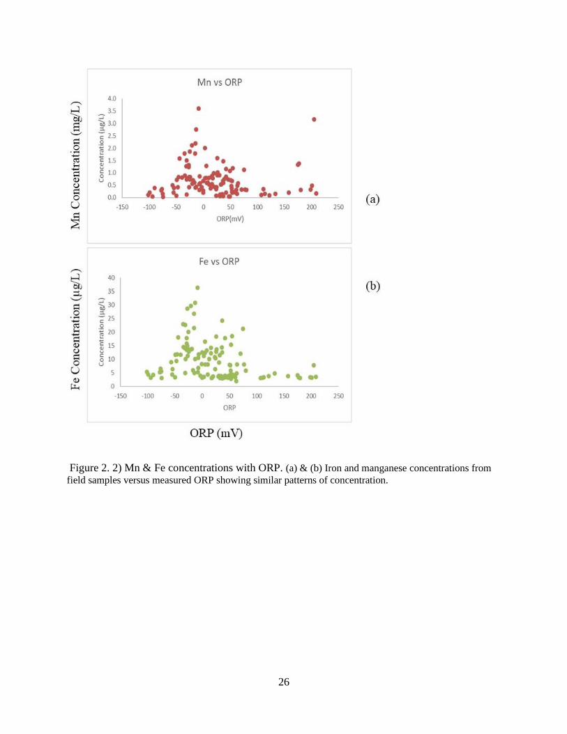
values range from 205 to -101 mV. Figure 2 a and b graphically illustrate Mn and Fe against

ORP, rendering a view of high transition metal concentration in suboxic to anoxic waters. Mn

and Fe concentrations against ORP indicate redox potential environments dominantly preferable

for nitrate and metal reduction (Brettar et al., 2002; Salazar et al., 2013) heavily suggesting

microbially mediated processes controlling these key groundwater constituents.

Figure 2.3 a and b illustrate Mn and Fe concentrations that are most abundant just below

neutral pH values and significantly decline at both high and low pH. Mn exhibits a slightly

higher soluble concentration than Fe at decreasing pH, as is to be expected. It is well documented

that iron oxides are far less soluble than manganese oxides, thus, it is natural to find higher Mn

concentrations in solution e.g. (HEM, 1972). This suggests lead removal is instigated by sorption

processes pertaining to Mn and Fe particles. Studies performed by O’Reilly (2003) and Trivedi

(2003) indicate preferred Pb sorption to Mn oxides and Fe oxides as a function of pH. Pb

sorption curve, given by Drever, describes Pb adsorption to Fe hydrous oxides (2002). A

fundamental key to adsorption is pH and Pb’s optimal adsorption pH value is 5.5 (Drever, 2002).

20

Microbial rate reactions of Pb sorption to Fe and Mn exceeds the rate of Pb dissolution during Fe

and Mn reduction. Indicating the reason behind Pb’s continued sorption under reducing

conditions.

Sulfate concentrations are spread throughout pH ranges of sampled water as shown in

Figure 2.4. Concentrations are noticeably absent above pH 7. Slightly below neutral pH,

however, Mn, Fe, and SO42- concentrations are all seen declining, coincidentally at the lowest

ORP values in the region. Sulfur reduction processes are likely occurring given the low ORP

values. Sulfide scavenging of Fe and Mn ions via sulfide minerals is therefore possible.

Ramamoorthy (2009) showed that Fe is easily retained in the mineral phase under anoxic sulfidic

conditions. Jones (2011) discusses Mn reactivity in the presence of sulfide is like that of Fe and

Mn. Sulfide minerals are therefore possible in bottom waters with present concentrations of

sulfide. In reduced waters, sulfide minerals are also known to collect heavy metals through

adsorption processes (Jean and Bancroft, 1986). Precipitation of PbS is kinetically faster than

their pyritization into Fe sulfide minerals (Morse and Luther, 1999). The exact sequestration

mechanism (adsorption or coprecipitation) of heavy metals via sulfide minerals in most natural

systems is questionable (Huerta-Diaz et al., 1998). Heavy mineral appropriation by sulfide

minerals is most likely occurring at high pH values. The determining mechanism is unknown and

is the subject of future research.

2.4 Spatial Analysis of Co-expression

Contour map constructs, modeled from analytical data and GPS coordinates, give a

comprehensive view of Kutupalong subsurface chemical interactions. The contour maps show

the spatial extent of selected constituents and their varying concentrations seen throughout the

21

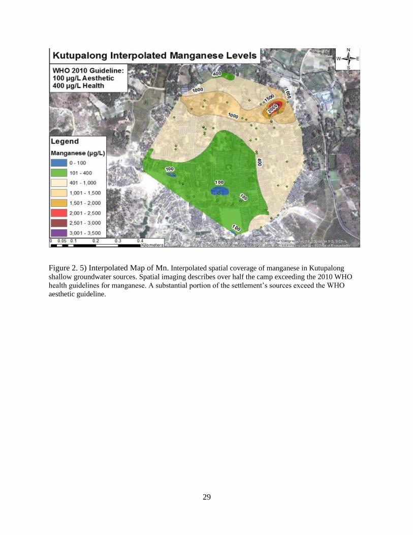
settlement. Figure 2.5 shows Mn concentrations meet or exceed world health organization

(WHO) aesthetic guidelines and established health parameters in nearly every region of

Kutupalong. Concentrations in the range of 100 µg/L to 400 µg/L are observed in the center of

the settlement spread through the southern and southwestern portion of the camp. Even higher

concentrations are observed throughout the rest of Kutupalong with a couple extreme levels

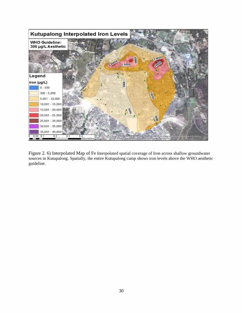
revealed in the northwest (Figure 2.5). Similarly, elevated iron concentration, are widespread in

Kutupalong simultaneously as well. Figure 6 illustrates the elevated iron spread in the settlement.

Every sampled water groundwater source exhibited iron levels above the WHO aesthetic

guideline of 300 µg/L.

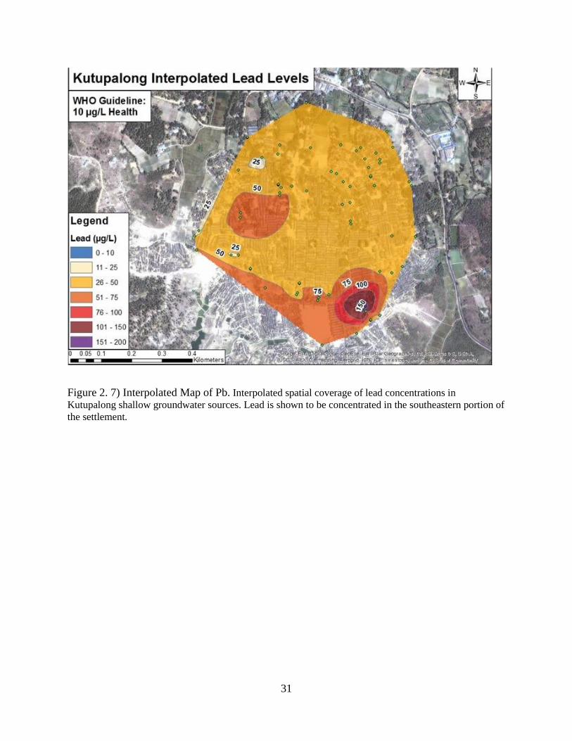
The map of Pb also shows values to be dominantly above the WHO health limit. Figure

2.7 gives the spread of Pb concentration in Kutupalong. Showing that Pb contamination is

heavily present in the camp’s subsurface. Figure 2.8 details nitrate concentration. Interestingly,

nitrate for the most part is not present in concerning levels. A few regions in Kutupalong do

exhibit levels of concern, however. In Figure 2.8 four regions are above the US Environmental

Protection Agency’s (US EPA) limit for nitrate.

Spatial analysis vividly highlights the relationships of Mn, Fe, and midrange pH in

regions of Kutupalong. Comparing Figure 2.2 to spatial Figures of 2.6, 2.7, and 2.9 not only

graphically is a trend seen between Fe and Mn at (5-7) pH, but spatial mapping further enhances

this bias. Figure 2.9 features pH resolution in Kutupalong and highlights the regions of sub

neutral pH. Thorough inspection of Figures 2.5 and 2.6, it is now spatially known that elevated

concentrations of Fe and Mn correspond to areas of (pH range 5-6.5) pH. Further solidifying the

graphical argument of an elevated pH generated by the reduction of Fe and Mn. The microbial

22

processes cause a rise in pH through the consumption of H+ while reducing Fe and Mn oxides

into solution.

In conjunction, spatial maps of NO3- and pH reveal overlaps of low pH with elevated

NO3- concentrations. Figures 2.8 and 2.9 show the spatial expression of nitrate and pH

respectively. While there is spatial variance in correlation, most of the high nitrate zones

demonstrated in Figure 2.8 do correspond to low zones of pH shown in Figure 2.9. Similarly,

spatially resolved aqueous lead concentrations (Figure 2.7) correlate well to spatially resolved

pH values (Figure 2.9). Nitrogen cycling is the controlling process in this pH - ORP zone. Also,

Pb follows this pH trend. Figure 2.7 illustrates Pb expressions resonate with NO3-, Fe, and Mn

zones. Indicating Pb sorption to Fe and Mn are dictated by pH changes caused by nitrogen

cycling.

The spatial correlation between Pb and NO3- is beneficial for public health developmental

management. Summation of spatial concentrations can be synthesized into spatial resolutions of

both elements depicting a net impact of concentrations in Kutupalong. Producing a spatial net

impact modeling elevated subsurface concentration as well as predicting areas of concern for

contaminant release. Risk assessment mapping can model overlapping concentrations of multiple

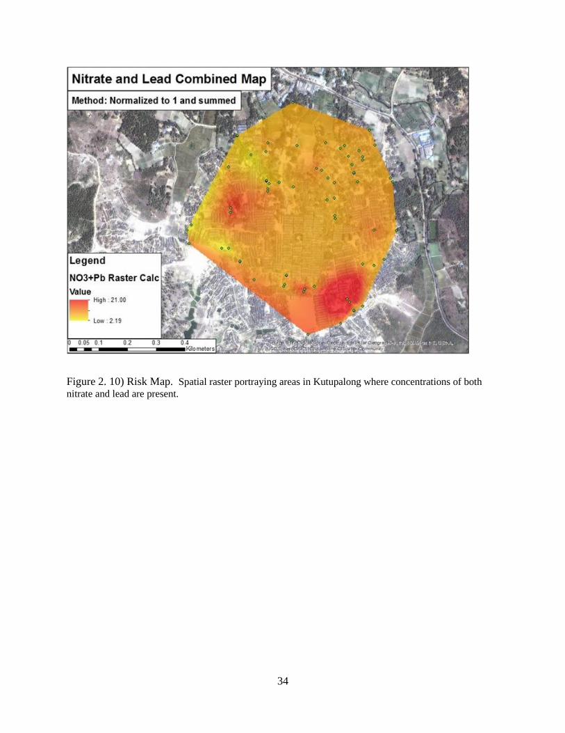
contaminants to predict subsurface areas for optimal use. Figure 2.10 depicts the combined Pb

and NO3- spatial coverage. This combined map can be used as a guidance tool to optimize the

geolocations of water points for sound usage.

2.5 Conclusion

Kutupalong settlement provides potable water for an increasing population of displaced

people. It is thus a public health concern and needs to recognize the quality of water being

23

delivered to the settlement’s population. Analyses revealed co-expression that ultimately

explains the release of contaminants into the drinking water system. Nitrogen cycling yielding

the formation of nitrate is shown to control pH by the release of paired hydrogen ion. Nitrogen

mediated pH levels control the surface charge of iron and manganese oxyhydroxide minerals and

thereby the sorption and desorption of surface-bound contaminants. Desorption of Pb from Mn

and Fe hydroxides leads to Pb availability in Kutupalong’s drinking water. While Pb

concentrations are well correlated with low pH and high nitrate, the observed co-expression is

spatially heterogeneous.

Non-point source contamination problems are challenges that require unique mitigation

strategies. Chemical sampling in Kutupalong has shown that not just Pb, but other contaminants

of concern are intermittently widespread throughout the settlement. While contaminations are

widespread, solutions are possible. Proper management of source contamination for nitrate is

possible and would greatly influence the subsurface chemistry. Limiting nitrogen input, such as

fertilizer runoff and animal waste, would help reduce nitrogen cycling driven pH drops in the

groundwater. This cuts the risk posed by direct contamination of NO3-, the pH driven dissolution

of available Mn, and the pH-controlled desorption of Pb from oxyhydroxides. Risk assessment

maps are an alternative strategy capable of identifying, accounting for, and avoiding

contaminated areas. Interpolated spatial models give users the ability to identify current and

potentially hazardous areas allowing a more complete examination of assessed contaminants. If

needed, spatial referencing can help strategically determine if existing wells should be closed and

avoided as well as a tool for determination of future well placement to accommodate incoming

populations. The developed spatial technique is a valuable method to assist in solving the crisis

in Bangladesh. Not only would using spatial techniques regionally help mitigate local issues but

24

using on a global scale would help facilitate proper responses to current and future

environmental and public health crises.

25

2.6 Figures and Tables

Figure 2. 1) Pb & NO3- concentration with pH. Measured concentration of soluble lead and

nitrate sampled in Kutupalong. (a) Elevated lead levels are uniformly released at pH values

around 4 and decrease as the pH rises to circumneutral where soluble lead levels are nearly

absent. (b) High nitrate levels are most noticeable at pH values slightly above 4. Nitrate

concentrations decrease as the pH rises barring a few outliers.

26

Figure 2. 2) Mn & Fe concentrations with ORP. (a) & (b) Iron and manganese concentrations from

field samples versus measured ORP showing similar patterns of concentration.

27

Figure 2. 3) Mn & Fe concentrations with shifting pH. (a) & (b) Measured soluble manganese and

iron concentrations. Both elements mimic each other in terms of their highest concentrations are optimal

near a pH of 6. Iron and manganese levels subside at pH values on either side of 6.

28

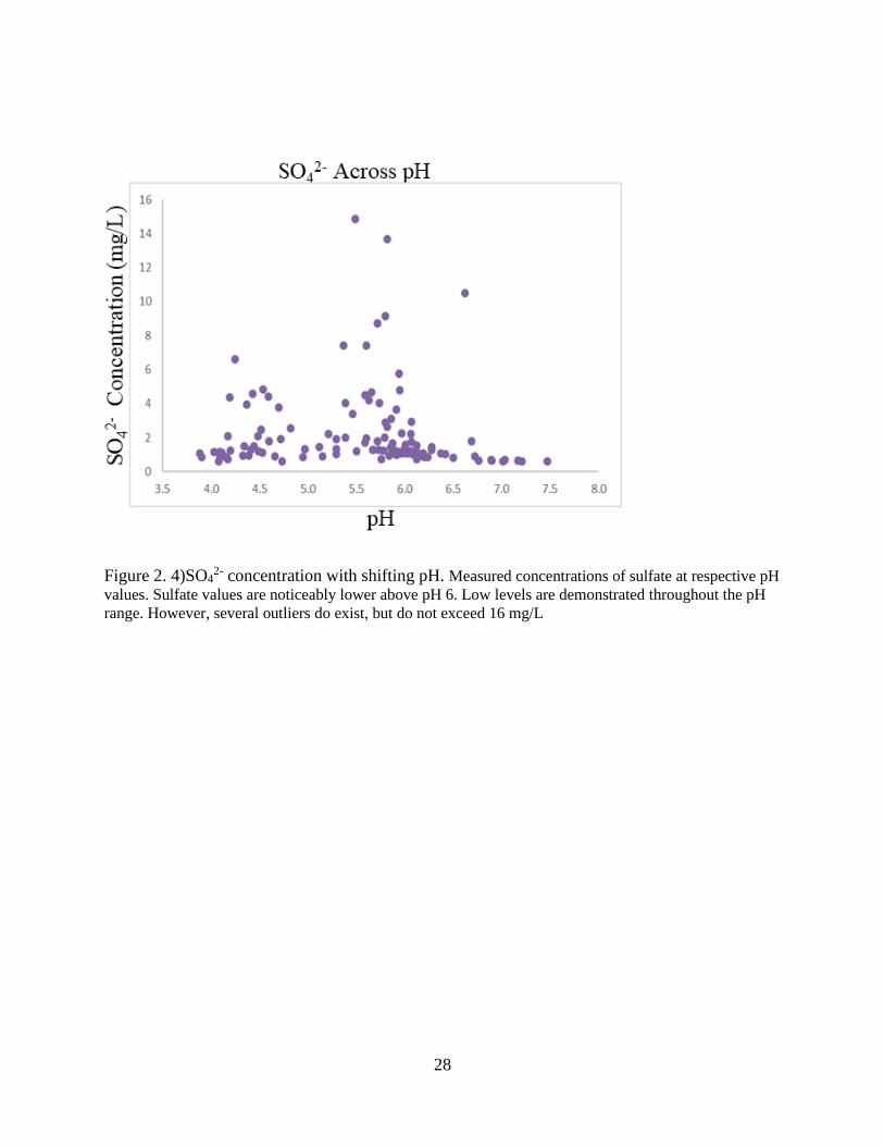
Figure 2. 4)SO42- concentration with shifting pH. Measured concentrations of sulfate at respective pH

values. Sulfate values are noticeably lower above pH 6. Low levels are demonstrated throughout the pH

range. However, several outliers do exist, but do not exceed 16 mg/L

29

Figure 2. 5) Interpolated Map of Mn. Interpolated spatial coverage of manganese in Kutupalong

shallow groundwater sources. Spatial imaging describes over half the camp exceeding the 2010 WHO

health guidelines for manganese. A substantial portion of the settlement’s sources exceed the WHO

aesthetic guideline.

30

Figure 2. 6) Interpolated Map of Fe Interpolated spatial coverage of Iron across shallow groundwater

sources in Kutupalong. Spatially, the entire Kutupalong camp shows iron levels above the WHO aesthetic

guideline.

31

Figure 2. 7) Interpolated Map of Pb. Interpolated spatial coverage of lead concentrations in

Kutupalong shallow groundwater sources. Lead is shown to be concentrated in the southeastern portion of

the settlement.

32

Figure 2. 8) Interpolated Map of NO3-. Interpolated spatial coverage of nitrate levels in Kutupalong

shallow groundwater sources. Imaging depicts concentrated areas of elevated nitrate contamination.

33

Figure 2. 9) Interpolated Map of pH. Interpolated spatial imaging of pH levels in Kutupalong. Much of

the settlement is outside the typical pH range for drinking water.

34

Figure 2. 10) Risk Map. Spatial raster portraying areas in Kutupalong where concentrations of both

nitrate and lead are present.

35

CHAPTER 3

Impact of Local Groundwater Conditions on Solid Speciation and Associated Soil-Water

Partitioning of Toxic Trace Metals in Bugesera, Rwanda

To be submitted to Applied Geochemistry

Abstract

Rwanda’s Bugesera district is a semiarid region in the country’s southeast. The district

possesses numerous lakes and other surface water bodies, but local populations in remote areas

rely primarily on hand-pumped shallow groundwater. Water quality monitoring in 2012 and

2014 lead to the discovery of several elevated metals in the region’s groundwaters. The potential

release or exposure of these heavy metals is a concerning issue for much of the population,

especially in the remote sectors of the district. It is well known that changes in soil-water

partitioning can lead to the subsurface release of heavy metals such as, in this case, manganese,

uranium, and vanadium. Here, mechanisms of spatially heterogeneous release are explored via

solid-phase speciation analysis of locales with varying groundwater dynamics.

2016 and 2017 sediment sampling determined that various regions in Bugesera

experience diverse levels of elevated metal concentrations leading to very different potential

mechanisms of release into the environment. Three handpump sites, within Bugesera, are

sampled and evaluated for solid concentrations of manganese, uranium, and vanadium. Depth-

resolved solid-phase sampling from each location revealed subsurface characteristics unique to

each site. Site1 shows a redox shift at the water table. Samples from Site2 are completely

collected from the vadose zone. While Site3 also reveals a redox shift, at the water table, but

with differing subsurface results from Site1. Sequential extraction experiments were completed

36

on each sample to understand metal solid speciation. Loss on ignition, calcination, and soil

acidity are techniques used to quantify associated soil components that can impact metal

speciation. These data combined can guide the biological availability and mobility of the metals

in question. This study aims to examine elevated metal concentrations in the subsurface and to

determine the mechanisms of potential release into the environment via solid-phase speciation.

Understanding these geochemical processes will allow for Bugesera to safely develop and

expand its economic potential by addressing metals risks before and during development as

opposed to reacting to future problems.

37

3.1 Introduction

Bugesera is a region within Rwanda’s eastern province, containing a geomorphology

leading to numerous lakes and wetlands. Though containing more surface water than regions to

the west and north, the region is semiarid and has been known to be impaired by drought

(Rwanyiziri and Rugema, 2013). For all the surface water present in Bugesera, many

communities historically rely on shallow, groundwater sources. Groundwater sources provide a

natural barrier to microbial contamination. Surface water, however plentiful, is nominally not

suitable for human consumption without treatment rendering groundwater sources even more

valuable to local communities.

2012 and 2014 water quality monitoring in Bugesera, Rwanda, uncovered toxic metals

in shallow aquifer drinking water systems. Uranium, and especially manganese, were established

at toxic levels in several drinking water sites across the district. These findings prompted further

investigation into the soil-water interface throughout the region. Excursions in 2016 and 2017

provided sediment samples, from select Bugesera groundwater sites, further highlighting the

presence of potentially harmful elements.

Manganese is a transition metal associated with numerous environmental processes in the

subsurface. Geochemically, it is an important element that, even at elevated concentrations, is

nominally seen as a harmless environmental pollutant. Previous World Health Organization

(WHO) guidelines, however, recommended manganese levels under 400 µg/L. These guidelines

have since been discontinued, on the insistence that manganese is only a health concern at and

above 400 µg/L and is rarely available in drinking water at such concentrations (World Health

Organization, 2011). 2012 and 2014 water quality monitoring in Bugesera, Rwanda noted in-use

drinking water boreholes containing significant amounts of manganese. Several sites far

38

exceeding the 400 µg/L guideline. High manganese concentrations are not unique to the East

African Rift Valley. Globally, numerous drinking water sources exceed 400 µg/L leading

manganese to be of a public health concern (Frisbie et al., 2012) with heightened exposure

leading to manganese toxicity, despite the shift in stance of WHO.

Concerns with uranium, as an environmental pollutant, are mostly owed to its radioactive

nature. Historically, uranium has been considered a major component of nuclear power

(Domingo, 2001). Uranium, though, is a toxic heavy metal with numerous ecological and public

health concerns separate from any radioactivity concerns (Selvakumar et al., 2018). Elevated

concentrations were found in Bugesera’s drinking water sources. It is therefore important to

investigate the dynamics in the subsurface of naturally occurring uranium.

Vanadium is an understudied, transitional metal of growing importance. It is used in

many industrial services such as petroleum refining, steel processing, and as a catalyst for the

reduction of NOx gasses (Bredberg et al., 2004; Imtiaz et al., 2015). From an environmental

standpoint, vanadium is becoming increasingly more important (Imtiaz et al., 2015). There is

debate on the toxicity risk vanadium poses, but vanadium contamination is a concern and should

be studied and assessed.

Essential to understanding the release dynamics for manganese, uranium, and other

potentially toxic metals, is their solid-solution partitioning. Metal bioavailability is not solely

determined through the sheer abundance of metallic concentrations in contaminated soil (Sauvé

et al., 2000). Potential environmental and public exposure, by metal availability, is thus a

determinant of multiple subsurface factors including soil acidity, soil organic matter, and soil

redox potential )(McBride et al., 1997; Roychoudhury and Starke, 2006).

39

This study aims to examine the chemical constituents controlling soil-water partitioning

to categorize and determine the potential release mechanisms of toxic metals in the region. It also

looks to investigate the bioavailability and mobility of constituents that are variably expressed in

the region.

3.2 Methods

3.2.1 Soil Coring

Soil core samples were collected using a 30 cm stainless steel push corer. Standard soil

sampling method was applied. Following site determination, the corer was pushed into the

sediment as far as it could via hand and rubber mallet. Samples were taken from softer sites

where the corer could be fully extended into the sediment. After the initial sample was collected,

a 30 cm length is added to extend the corer’s reach. Multiple lengths were added until core depth

exceeded the groundwater table, or all lengths were used. For a sample core, each core length

denotes a depth fraction for that sample. Each depth fraction is further subdivided. The top inch

to 5 in and the bottom 5 in of the fraction was discarded. The remaining sediment was removed,

intact from the corer’s barrel by a stainless-steel spatula, and homogenized on aluminum foil.

The depth fractionated homogenized sample was then collected in a 50 ml centrifuge tube.

3.2.2 Sequential Extractions

A sequential extraction procedure modified from Tessier and coauthors was used to

quantify speciation of elements of interest in the collected sediment core depth fractions (Tessier

et al., 1979). Species from the four most environmentally relevant fractionation phases were

40

measured. Phase 1 determined the exchangeable cations from the sampled sediment. 0.5 grams

of dried sample is placed in a 50 ml centrifuge tube. 8 ml of 1 mol/L MgCl2, at pH 7, solution

was then added to the centrifuge tube. The sample was extracted for one hour on rotators.

Following the extraction, and each following extraction, the mixture was centrifuged at 4000

rpm for 5-10 minutes to compact the remaining sediment. The extractant is poured off and

prepped for ICP-MS analysis.

Phase 2 obtained analytes bound to the carbonate fraction of the sediment. 8ml of 0.1

mol/L sodium acetate, adjusted to pH 5 with HNO3, was added to the residual of phase one.

Phase 2 is extracted for 5 hours on rotators. Following extraction, the sample is centrifuged at

4000 rpm for 5-10 min. The extricated solution is poured off and prepped of ICP-MS analysis.

Phase 3 was intended to target analytes bound to the poorly crystalline iron and

manganese oxides. 20 ml of 0.1 mol/L hydroxylamine hydrochloride, adjusted to pH 2 via

HNO3, was added to the residue from phase 2. The reaction ensued for 16 hours, while on

rotators. Next, centrifugation at 4000 rpm occurred and the extracted solution was poured off for

ICP-MS preparation.

The final extraction, phase 4, targeted analytes bound to organic matter. The residual

from phase 3 was combined with 3 ml of 0.02 mol/L HNO3 and 5 ml of 30% H2O2 at pH 2. The

mixture was extracted for 1 hour on rotators. The mixture was then placed in a preheated hot

block at 85 °C for 1 hour. This phase 4 process was repeated once more. The extracted material

was diluted with 5ml of 1 mol/L HNO3, and finally poured off and prepared for ICP-MS

analysis.

41

3.2.3 Loss on Ignition

A loss on ignition (LOI) analysis determined the organic matter content in the sediment

core samples. Representative depth-resolved samples, from each core, were dried in an oven

around 100°C for 1 hour, driving off any water. The sample was then massed, to gain the weight

of dry mass, and placed in a pre-massed ceramic crucible. Following measurement, each sample

was placed in the furnace at a temperature of 550 °C for 1 hour to oxidize organic matter to CO2.

Each crucible was then removed and allowed to cool in a desiccator until room temperature was

reached. Once cooled, the crucible containing the sample was massed again. The differential

mass loss can be attributed to the amount of organic material in each sample (Walter E. Dean,

Jr., 1974). An equation for LOI is given by (Heiri et al., 2001):

LOISOM = (𝑀𝑑𝑟𝑦 − 𝑀550)

𝑀𝑑𝑟𝑦× 100

Where,

LOISOM = the mass differential of organic material.

Mdry = the mass of the dried solid at 100°C

M550 = the mass of the solid at 550 °C

3.2.4 Calcination

Calcination is a continuation of LOI. A modified calcination analysis was used to

determine the carbonate fraction. Samples previously measured in LOI analysis were then placed

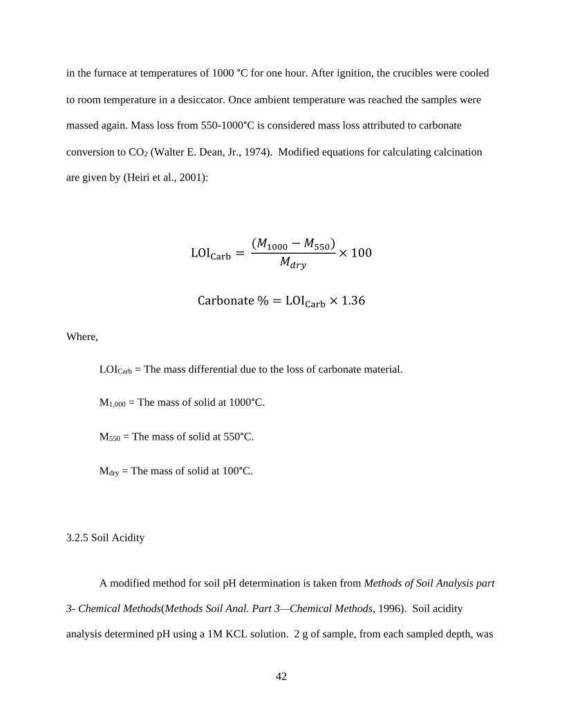
42

in the furnace at temperatures of 1000 °C for one hour. After ignition, the crucibles were cooled

to room temperature in a desiccator. Once ambient temperature was reached the samples were

massed again. Mass loss from 550-1000°C is considered mass loss attributed to carbonate

conversion to CO2 (Walter E. Dean, Jr., 1974). Modified equations for calculating calcination

are given by (Heiri et al., 2001):

LOICarb = (𝑀1000 − 𝑀550)

𝑀𝑑𝑟𝑦× 100

Carbonate % = LOICarb × 1.36

Where,

LOICarb = The mass differential due to the loss of carbonate material.

M1,000 = The mass of solid at 1000°C.

M550 = The mass of solid at 550°C.

Mdry = The mass of solid at 100°C.

3.2.5 Soil Acidity

A modified method for soil pH determination is taken from Methods of Soil Analysis part

3- Chemical Methods(Methods Soil Anal. Part 3—Chemical Methods, 1996). Soil acidity

analysis determined pH using a 1M KCL solution. 2 g of sample, from each sampled depth, was

43

massed out and placed in a 15ml centrifuge tube. 2 ml of 1M KCL is added and mixed to the

sample. The mixture is rested for ten-minutes, then measured with a pH meter and probe. The pH

is recorded as pHKCl (Methods Soil Anal. Part 3—Chemical Methods, 1996).

3.2.6 Inductively Coupled Plasma Mass Spectrometry

Solution phase metal concentrations were analyzed using a Thermo Fisher Scientific,

Thermo X-Series 2 ICP-MS. The instrument used a 5% HNO3 matrix, prepared from trace metal

grade concentrated 65-70% nitric acid and 18.2 mΩ Nanopure water. Analytical measurements

were completed using collision cell technology with kinetic exclusion discrimination (CCT-

KED) mode. Samples were diluted with and the same 5% HNO3 matrix described above to

adjust to the calibration concentration range of 0.5 µg/L to 100 µg/L. A blank sample, composed

of the 5% HNO3 matrix, was measured every ten to fifteen samples. Blanks were used to verify

sufficient washout time between sample runs and to monitor drift during instrumental analysis.

Instrument calibration used standards ranging from a concentration of 0 to 100 µg/L. High-

quality standards were prepared from SPEX CertiPrep Multi-Element Solution 2A diluted into

5% HNO3. Calibration curves with an R2 of .999 or higher were used in combination with blank

subtraction and dilution factors to convert uncorrected instrumental values to concentrations.

3.3 Results

The results of this study are divided into three locations where each sediment core was

sampled. Each sample site is located near a groundwater handpump and within an area of use by

44

a local community. Each analyte at every location was summarized into individual five-number

summaries. Each one found in the appendix.

3.3.1 Lowland Swamp

Samples cored from the initial Site1 location were cored from a lowland swamp, where

previously sampled groundwater showed elevated manganese in solution. Groundwater sampling

characterized soluble manganese well above, at the time, WHO Guidelines for manganese in

drinking water. Manganese was found to be 622µg/L in the pore water. The site was thought to

be potentially comprised of an abundance of manganese minerals due to the high manganese

concentrations in the pore water. Table 3.1 characterizes the soil acidity. The soil pH trends to

acidic levels with depth. Near-surface pH values are circumneutral while values at depth reach

pH values of 4.6. Figure 1 describes the SOM with descending depth. A visible trend that shows

the percentage of organic matter gradually increases with depth, even as depth descends past

groundwater. Figure 3.2 graphically describes the five-number summary for SOM above and

below groundwater. Relating an increase of SOM below the groundwater. The sediments’

carbonate material is shown not to have a clear trend with Figure 3.1. Though Figure 3.2 uses the

five-number summary to show that there is a higher average percent of carbonate material below

the water table.

Figure 3.6 demonstrates the abundance of various species of manganese sampled from

Site1’s sampled core. The figure shows manganese is present in large quantities in various solid

species, with the most prevalent speciation occurring as manganese oxides. Organic matter and

carbonates phase species are also at noticeably high concentrations. At near-surface,

45

concentrations decrease steadily with depth. Below groundwater (45-50 cm), concentrations

rapidly decline to near zero. Figure 3.7 depicts manganese absolute concentration and

concentration per phase, by depth, in each core. While the lower plot of Figure 3.7 illustrates the

fractional percentage of manganese concentration by phase. Analysis shows manganese exist in

high levels in the surrounding soil, but unlike the other analytes, it is not concentrated in the

organics. Manganese exists heavily in its oxide form (MnIV) but also as an exchangeable

divalent cation (Mn2+).

Figure 3.8 indicates uranium speciation and depicts solid uranium concentrations that are

most viable in the carbonate phase along with the soil organic matter. Figure 3.8 shows an

increasing trend with depth. Surface concentrations are near zero and gradually increase until

groundwater is reached. At a saturated depth, uranium values take a significant jump in solid

concentrations. The upper plots of Figure 3.9 illustrate the absolute concentrations of uranium

observed at the lowland marsh. The plots further illustrate the mineral phase speciation of

uranium obtained from sequential extraction experiments. The lower plots describe the uranium

percentages found in each of these extracted phases confirming the analysis of Figure 3.9 that

solid uranium concentration is mostly found in the organic and carbonate phases.

Vanadium speciation at the sampled site is described in Figure 3.10. Vanadium is mostly

present while bonded to SOM showing a trend of decreasing concentration with depth. Absolute

abundance and vanadium speciation percentage are both described in Figure 3.11. Vanadium

concentrations are at significant levels throughout the soil profile; however, they are focused in

the SOM.

46

3.3.2 Mining Hill

The sample cored near a mining hill, Site2, was done so at a decommissioned borehole.

Groundwater previously sampled near location was found to have excessive levels of metals,

most noticeably uranium. Previous studies characterized uranium at 420µg/L. The WHO

guideline is 30 µg/L. The well was decommissioned due to poor quality. The entire set of lengths

were added to the instrument during sampling of this core (266cm). Notably, groundwater was

never reached. Soil acidity, as shown in Table 3.1, is maintained around pH 6 with near-surface

depths hitting slightly acidic pH values. Figure 3.1 shows the percentage of SOM and carbonate

material. While Figure 3.3 illustrates the five-number summary of SOM and carbonate material.

Depth correlations with organic matter and mineral carbonate are not observed.

Manganese is shown to be elevated at this location, though not at the same concentrations

observed from the previous site. Figure 3.12 indicates significant amounts of manganese in the

oxide form relative to other species. The depth-resolved absolute concentrations and speciation

of manganese are given in Figure 3.13.

What little uranium found on the solid is focused on the organic and carbonate phases.

Figure 3.14 illustrates the uranium speciation and concentration for site Site2. Figure 3.15

describes the absolute concentration and percentage of uranium speciation further describing

what is seen in Figure 3.14.

47

Figure 16 reveals vanadium trending with depth. Vanadium is mostly bound to the

organics but also with the oxides. Figure 3.17 further breaks down vanadium concentration and

speciation with depth.

3.3.3 Agricultural Field

The sample taken from an agricultural field was cored from a setting without prior data.

Not much was known about this site. Water produced at this site is described as having a salty

taste and aesthetically unpleasing appeal. A 67 cm core was sampled, where groundwater was

reached at depths of 33-40cm. Table 1 shows the inclination of the soil pH to increase with

depth. Depths above the groundwater contain acidic soils while neutral soils persist below.

Figure 3.4 details the SOM and carbonate material at this site. Further illustrated by Figure 3.5,

The boxplot of the five-number summary shows the sediments above groundwaters as having

higher percentages than those below groundwater. SOM and carbonates decrease with depth with

some outliers observed at groundwater.

Manganese observed at this site is far lower in solid concentrations than in the previously

examined locations. Figure 3.18 illustrates the perceived manganese solid concentrations found

in the agricultural field. Figure 3.19 outlines manganese speciation with depth also recording that

most manganese is found in the oxides. Uranium, at this location, is also present at low values on

the solid; however, it does decrease with depth as shown in Figure 3.20. Figure 3.21 shows

uranium movement with depth as absolute concentrations and uranium speciation. Solid

vanadium behaves similarly with depth as described in Figure 3.22. Vanadium is only observed

48

in two phases at this location. From Figure 3.23, vanadium is associated with the oxides and is

bound to the organic fraction.

3.4 Discussion

Chemical analyses define several geochemical trends within the Bugesera subsurface.

Many relationships are consistent with the known geochemistry of individualized analytes.

However, results are not constant across all sites for each subsurface expression. The three sites,

examined in this study, each express the variability of concerning elements’ bioavailability in a

manner unique to the localized subsurface area. Five-number summaries of each analyte from all

three locations are given in the appendix.

3.4.1 Manganese

Site1, the lowland swamp, is overwhelmed with manganese in the soil and groundwater.

Solid manganese is mostly observed as an oxide with concentrations steadily decreasing with

depth. At groundwater, (45-50 cm), solid manganese levels descend rapidly. Soil pH levels

above groundwater are 6 and above. At these pH levels, under oxidizing conditions, manganese

is known to form solids. Accordingly, Figures 3.6 & 3.7 show heavy manganese presence in

oxides and organic matter. In acidic and or reducing soils manganese is highly soluble, this being

observed in Figures 3.6 & 3.7 also. At and below groundwater, soil pH turns acidic

simultaneously with manganese solid concentrations nearing zero. This transition most likely

records solid MnO2 reducing to soluble Mn2+with depth. The difference in solid Mn found above

and below the groundwater was tested to be statistically significantly different with 95%

confidence according to t-Test Appendix Table 11-14.

49

At the mining hill location, manganese is present and found mostly in the oxides,

(Figures 3.12 & 3.13) but not in the solid concentrations seen previously at the manganese

inundated swamp. Soil acidity hovers around a pH 6, Table 3.1, optimal pH for manganese to

form solid complexes. The carbonate and organic matter at this location are low which is why

manganese oxides are the most abundant solid complex (Figures 3.1 & 3.3). In this sample, the

reduction of MnO2 to Mn2+ is not observed though it is likely the reducing process is taking

place at deeper depths once groundwater is reached.

The manganese interactions at and around the water-table denote a groundwater barrier

for a redox shift in the subsurface environment. Depths above groundwater are an oxidizing

environment, while the saturated zone presents reducing conditions. The groundwater table is

observed at both the lowland swamp and the agricultural field (Figures 3.6 & 3.18). Though the

sediment core obtained from the Site3 location was sampled past the groundwater table, similar

geochemical tendencies as the lowland sample are not recorded. Solid manganese is present at

far lower concentrations than previously examined. High levels of near-surface SOM would

indicate plenty of organic complexes for manganese to bind with at surface. The soil pH above

groundwater in the oxic zone, however, is too acidic for manganese complexation promotion.

Thus, manganese is far more soluble in this area and is not found in mineral form at the same

levels in preceding regions. It is likely, therefore, that Mn is soluble above the water table due to

acidity and below the water table due to the redox condition.

3.4.2 Uranium

50

Figures 3.8 & 3.9 describes uranium concentration, at the marshland, with depth. Noting that

solid uranium is not heavily present until groundwater. Uranium is soluble under oxic conditions

and highly insoluble in reducing ones. There is a change of uranium (VI) to uranium (IV) in the

reducing environment. This redox driven solubility shift is shown through the significant uptake

in uranium concentration with depth observed in Figures 3.8 & 3.9. With 95% confidence it is

concluded that there is a statistically significant difference between U above and below the

groundwater (Appendix Table 15-18).

The core taken from the mining hill was appropriated in a region where previous analysis

noted substantial groundwater uranium. It is believed that this region sits atop parent granite

rock, a potential source of considerable amounts of subsurface uranium. Given that the core,

sampled at this location, did not reach groundwater, it was not expected to see a redox shift in the

subsurface environment. Figure 3.14 depicts a near absence of solid uranium. Uranium being

highly soluble under oxidizing conditions is consistent with a lack of observed solid-phase

uranium. It is highly likely that the uranium here is present in the pore water and as U(IV) in the

deeper reducing environment.

Unlike the first locations sampled; uranium is nearly completely absent from the reducing

environment found in the agricultural field subsurface. As noted in Figures 3.20 & 3.21. This is

most likely due to this region not sitting atop granite parent material (Dewaele et al., 2010; Ghehi

et al., 2012)

3.4.3 Vanadium

51

Vanadium throughout the marshland region is found bound to organic matter. Solid

vanadium concentrations decrease with depth, even past groundwater (Figure 3.10). The

reducing conditions and the increase of SOM, at depth, does not change the declination of solid

vanadium. Vanadium’s solubility seems to be more affected by the increasingly acidic soil pH,

(Table 3.1 & Figure 3.11). Reducing conditions promote a reduction of vanadate V(V) to

vanadyl V(IV), increasing the ion’s solubility (Bredberg et al., 2004). Further, V (V) reduction to

(IV) increases the ions sorption propensity to SOM (Reijonen et al., 2016). Both trends are

supported by the low solid concentrations and the percentage of V in SOM shown in Figures

3.10 & 3.11. These trends are tested and proven with 95% confidence to be statistically

significant according to t-Test (Appendix Table 19-21).

In the subsurface of the mining hill region, vanadium is complexed on organic matter,

and found in lesser concentrations on the oxides. With depth, levels are decreasing on SOM and

increasing on the oxides, Figures 3.16 and 3.17. This is most likely because of the decrease in

organic material with depth. Figure 3.1 depicts a slight decrease with depth for SOM at this

location.

In the agricultural field, solid vanadium is seen declining in both SOM and oxides. The

declination can be attributed to the depth of diminishing organic material and the increase in soil

pH. A neutral to high pH means vanadium is more soluble, which is likely happening with

vanadium downturn at depth. It is also likely that a reduction of vanadate to vanadyl is taking

place after the environmental redox shift. Figure 3.22 displays this noticeable subsurface activity.

The collected samples demonstrate the diverse sediment and soil profiles within

Bugesera. The hypotheses of unique and significant trends, with depth, per elemental speciation,

were tested using a t-test with unequal variances. T-test indicates that there are statistically

52

differing spatial trends, with depth per heavy metal, from each sampled location. These t-tests

are completed with 95% confidence and can be found in Appendix A (Appendix Table 10-21). It

is expected to see differences in elemental expressions between saturated sediment samples

where groundwater is reached in one and a completely dry sample in the other. However, the

dissimilarities between saturated sediments collected in redox changing environments were

visible. This hypothesis was also proven using the t-test (Appendix Table 22-32). Differentials in

elemental expressions by these sediments are caused most notably by the changing soil acidity

and other physicochemical parameters. The changing soil pH combined with the depth varying

presence of SOM, carbonate material and redox shifting environments are controlling factors for

the highly differing elemental expressions in a relatively small spatial setting. Figure 3.1

describes SOM increasing in concentration with depth for the lowland swamp and the mining hill

regions. This trend, however, is not observed in the agricultural region as shown in Figure 3.4.

From the topsoil down, there is a decrease in the SOM in the agricultural subsurface. Other

notable reasons to the differing subsurface expressions are, the absolute abundance of elements

and physiochemical material in the subsurface as well as parent rock material. Shale is a

predominant parent rock material in the subsurface of the agricultural field (Ghehi et al., 2012).

3.6 Conclusion

Rwanda’s Bugesera region uniquely differs from the country’s more tropical climate

regions. It, however, is no less important to Rwanda’s future economic development.

Construction is already underway for a second international airport in Bugesera making regional

development the next step for Rwanda’s progress as an East African hub. With land development

comes public health and safety concerns. Transitioning Bugesera from an agrarian municipality

to a land developed region means potential for the environmental release of toxic bioavailable

53

chemicals. Bugesera development is a necessary progressive step, especially considering its

exceptional place in recent Rwandan history. Nevertheless, precautions must be taken with future

development. The interpretations of subsurface geochemical expressions described in this study

will go a long way into future land development in Bugesera.

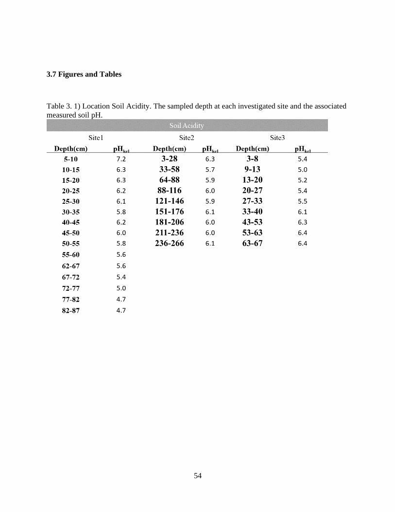
54

3.7 Figures and Tables

Table 3. 1) Location Soil Acidity. The sampled depth at each investigated site and the associated

measured soil pH.

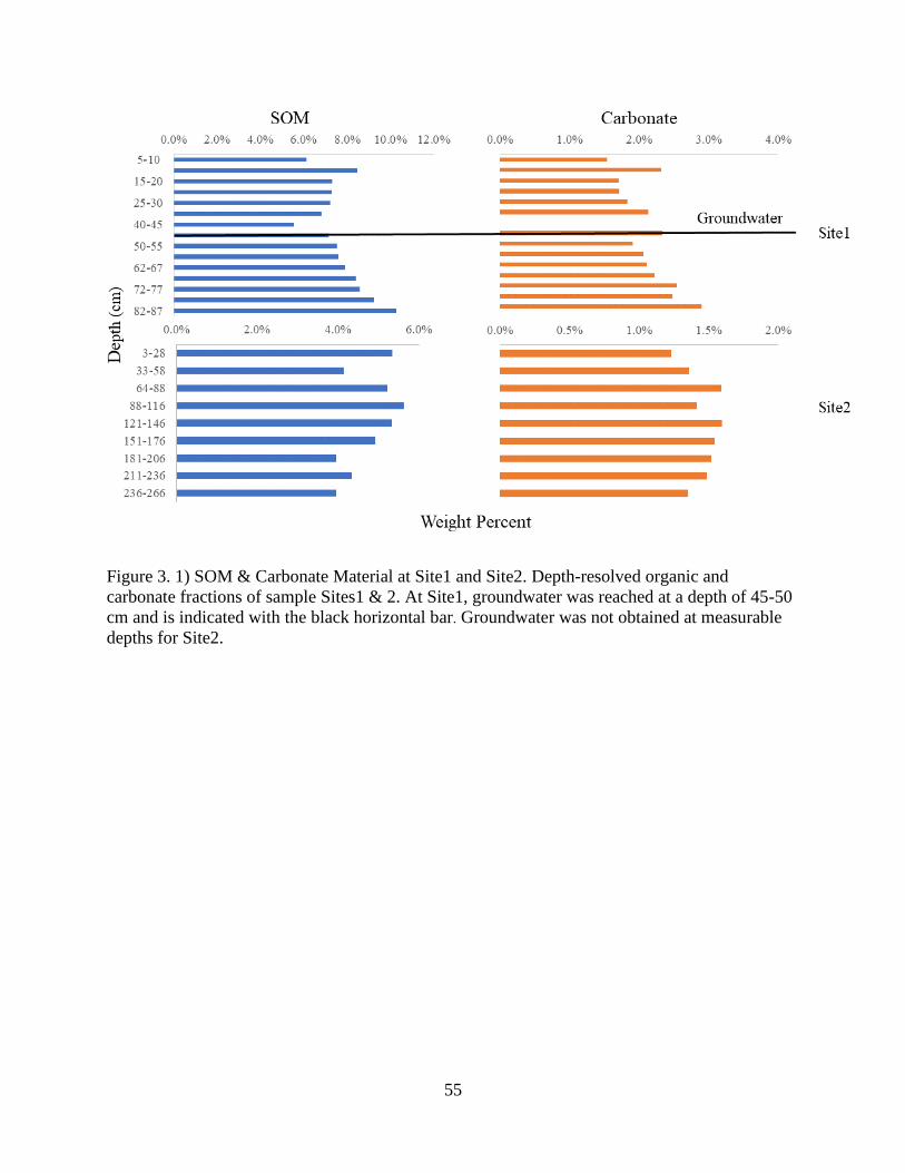
55

Figure 3. 1) SOM & Carbonate Material at Site1 and Site2. Depth-resolved organic and

carbonate fractions of sample Sites1 & 2. At Site1, groundwater was reached at a depth of 45-50

cm and is indicated with the black horizontal bar. Groundwater was not obtained at measurable

depths for Site2.

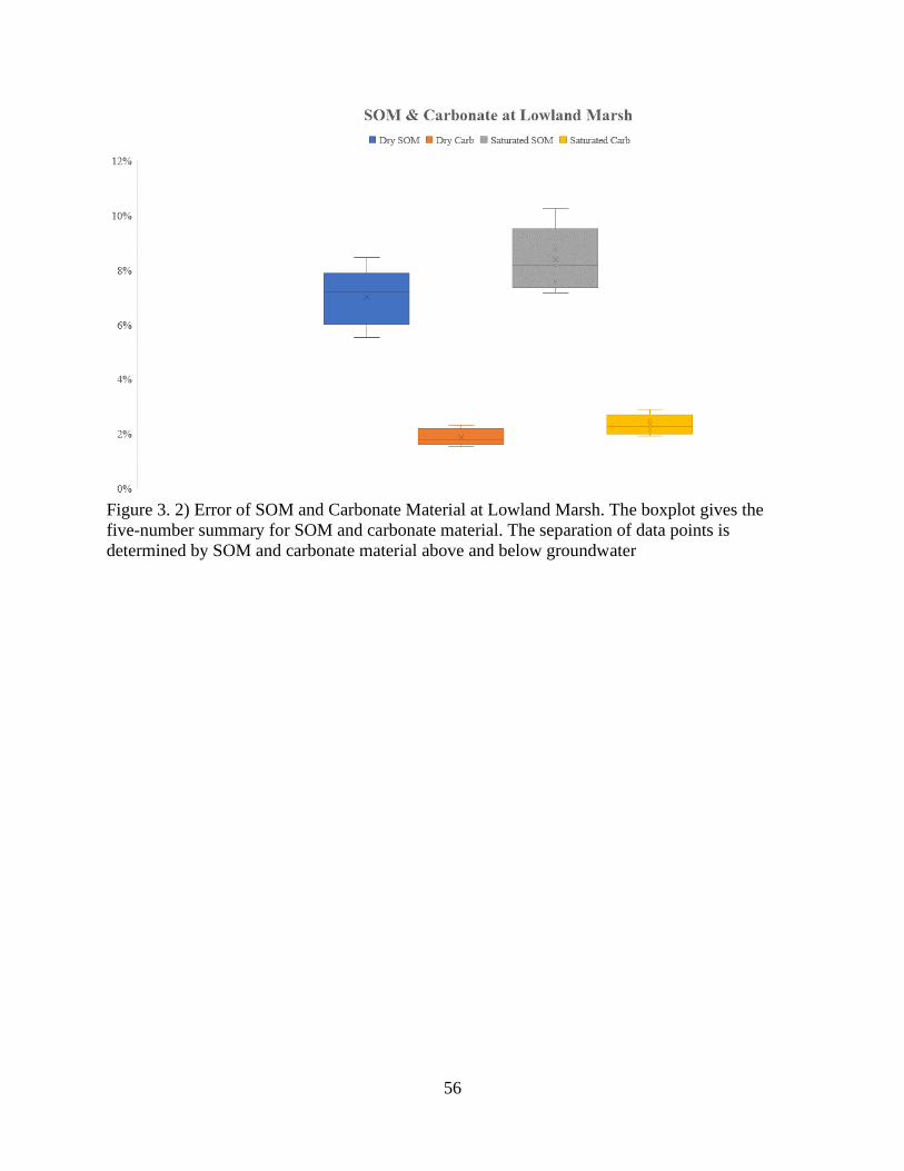
56

Figure 3. 2) Error of SOM and Carbonate Material at Lowland Marsh. The boxplot gives the

five-number summary for SOM and carbonate material. The separation of data points is

determined by SOM and carbonate material above and below groundwater

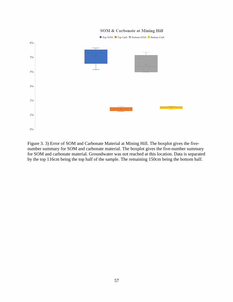
57

Figure 3. 3) Error of SOM and Carbonate Material at Mining Hill. The boxplot gives the five-

number summary for SOM and carbonate material. The boxplot gives the five-number summary

for SOM and carbonate material. Groundwater was not reached at this location. Data is separated

by the top 116cm being the top half of the sample. The remaining 150cm being the bottom half.

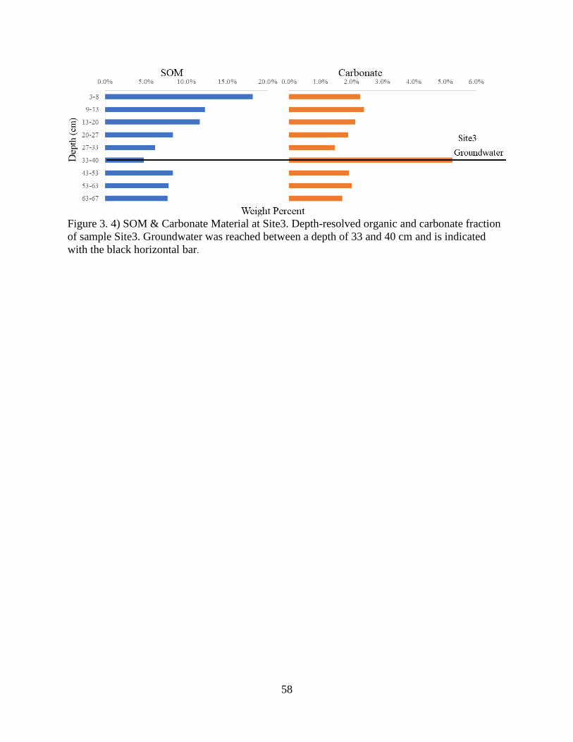
58

Figure 3. 4) SOM & Carbonate Material at Site3. Depth-resolved organic and carbonate fraction

of sample Site3. Groundwater was reached between a depth of 33 and 40 cm and is indicated

with the black horizontal bar.

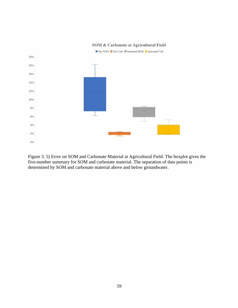
59

Figure 3. 5) Error on SOM and Carbonate Material at Agricultural Field. The boxplot gives the

five-number summary for SOM and carbonate material. The separation of data points is

determined by SOM and carbonate material above and below groundwater.

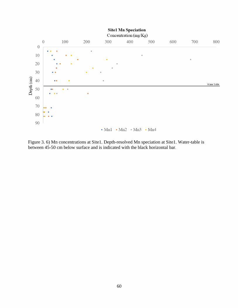
60

Figure 3. 6) Mn concentrations at Site1. Depth-resolved Mn speciation at Site1. Water-table is

between 45-50 cm below surface and is indicated with the black horizontal bar.

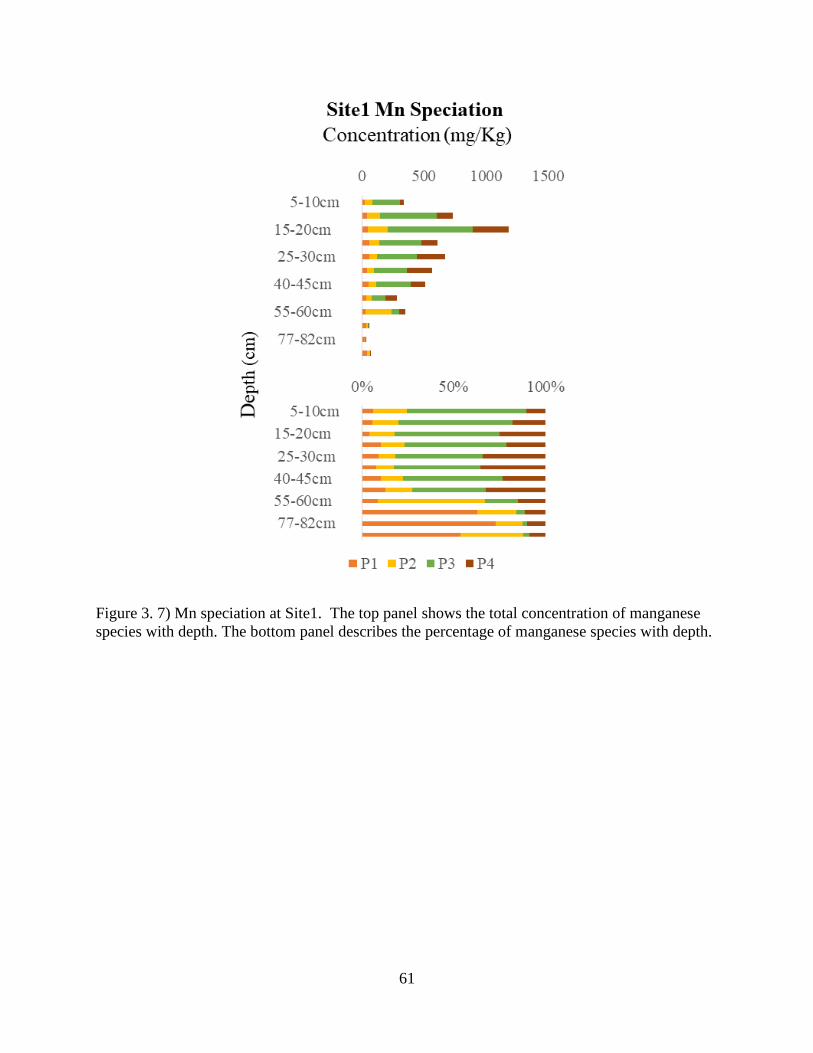
61

Figure 3. 7) Mn speciation at Site1. The top panel shows the total concentration of manganese

species with depth. The bottom panel describes the percentage of manganese species with depth.

62

Figure 3. 8) U concentrations at Site1. Depth resolve uranium speciation at Site1. Water-table is

between 45-50 cm below surface and is indicated with the black horizontal bar.

63

Figure 3. 9) U Speciation at Site1. The top panel shows the total concentration of uranium

species with depth. The bottom panel describes the percentage of uranium species with depth.

64

Figure 3. 10) V concentrations at Site1. Depth resolve vanadium speciation at Site1.

Groundwater is between 45-50 cm below surface and is indicated with the black horizontal bar.

65

Figure 3. 11) V speciation at Site1. The top panel shows the total concentration of vanadium

species with depth. The bottom panel describes the percentage of vanadium species with depth.

66

Figure 3. 12) Manganese concentrations at Site2. Depth-resolved manganese speciation for

sample Site2. Water-table was not found during sampling.

67

Figure 3. 13) Mn speciation at Site2. The top panel shows the total concentration of manganese

species with depth. The bottom panel describes the percentage of manganese species with depth.

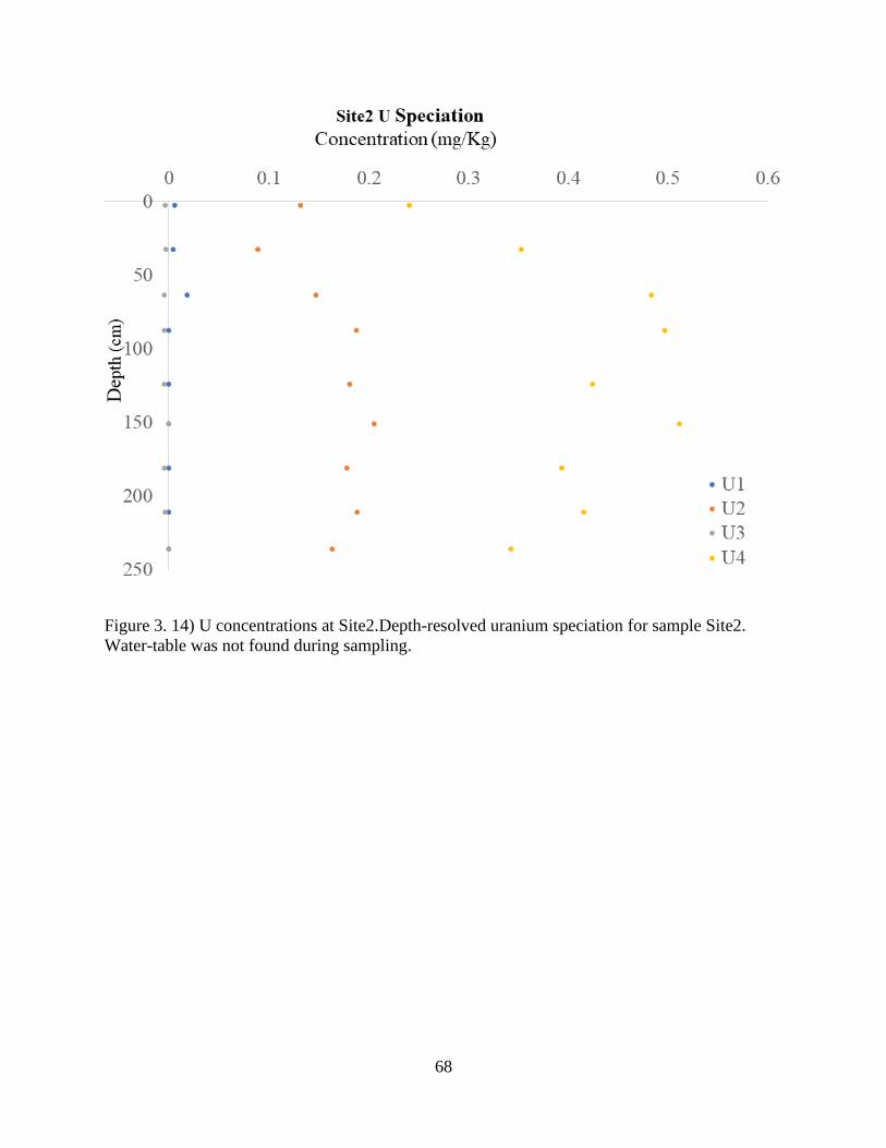
68

Figure 3. 14) U concentrations at Site2.Depth-resolved uranium speciation for sample Site2.

Water-table was not found during sampling.

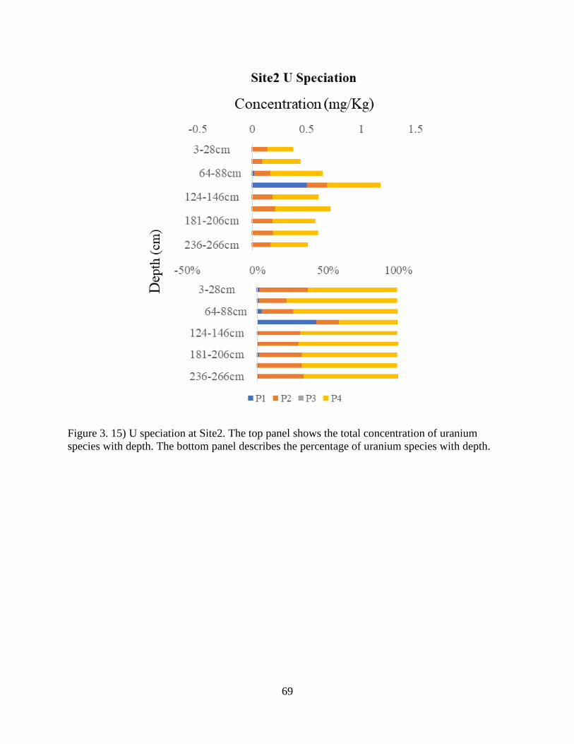
69

Figure 3. 15) U speciation at Site2. The top panel shows the total concentration of uranium

species with depth. The bottom panel describes the percentage of uranium species with depth.

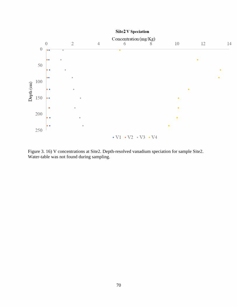
70

Figure 3. 16) V concentrations at Site2. Depth-resolved vanadium speciation for sample Site2.

Water-table was not found during sampling.

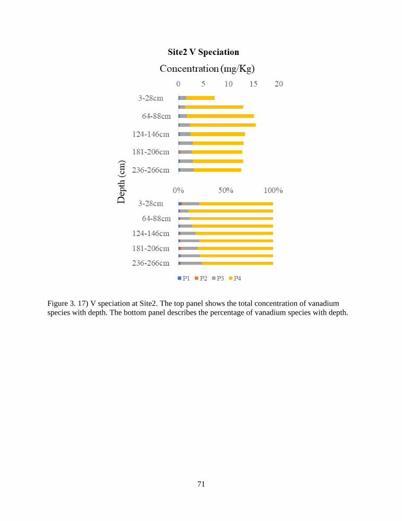
71

Figure 3. 17) V speciation at Site2. The top panel shows the total concentration of vanadium

species with depth. The bottom panel describes the percentage of vanadium species with depth.

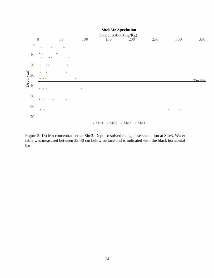
72

Figure 3. 18) Mn concentrations at Site3. Depth-resolved manganese speciation at Site3. Water-

table was measured between 33-40 cm below surface and is indicated with the black horizontal

bar.

73

Figure 3. 19) Mn speciation at Site3. The top panel shows the total concentration of manganese

species with depth. The bottom panel describes the percentage of manganese species with depth.

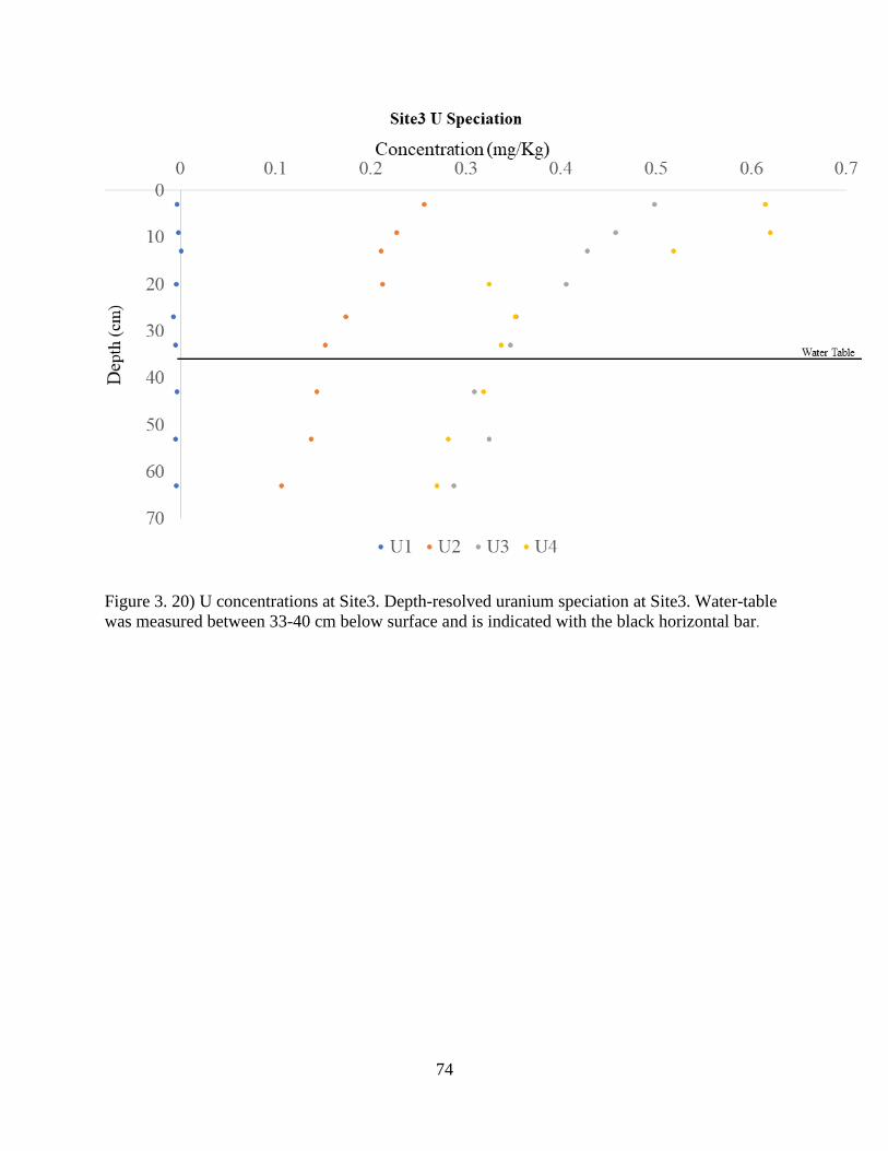
74

Figure 3. 20) U concentrations at Site3. Depth-resolved uranium speciation at Site3. Water-table

was measured between 33-40 cm below surface and is indicated with the black horizontal bar.

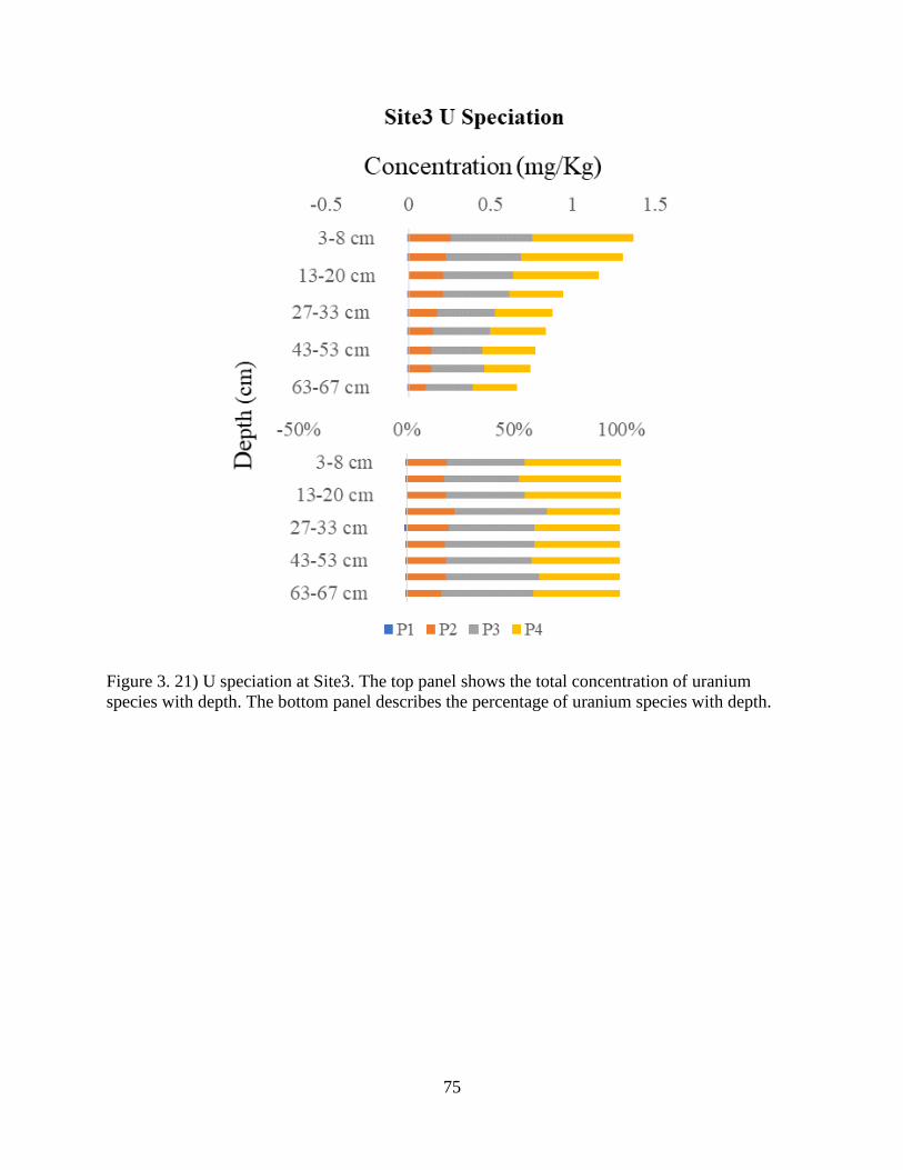
75

Figure 3. 21) U speciation at Site3. The top panel shows the total concentration of uranium

species with depth. The bottom panel describes the percentage of uranium species with depth.

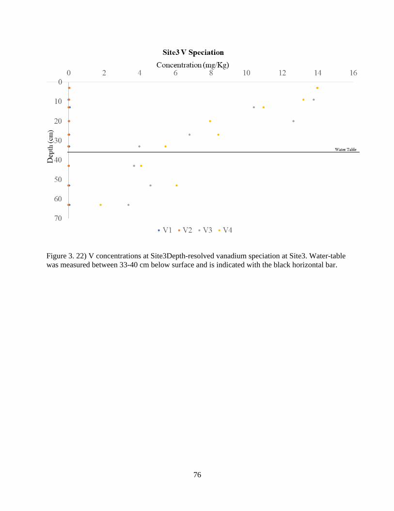
76

Figure 3. 22) V concentrations at Site3Depth-resolved vanadium speciation at Site3. Water-table

was measured between 33-40 cm below surface and is indicated with the black horizontal bar.

77

Figure 3. 23) V speciation at Site3. The top panel shows the total concentration of vanadium

species with depth. The bottom panel describes the percentage of vanadium species with depth.

78

CHAPTER 4

Inherent Toxicity Through Dispersion of Sized Determined Dust Particles in Bugesera, Rwanda

To Be Submitted to The Journal of Environmental Pollution

Abstract

Soils from tropical environments have a noticeably greater ability to collect, retain, and

concentrate heavy metals compared to soils from more temperate environments (Naidu et al.,

1998). Indeed, natural weathering commonly associated with tropical soils leaves behind soils

concentrated with trace and heavy metals (Rieuwerts, 2007). Therefore, either from naturally

occurring or anthropogenic sources, tropical soils are a vast potential source for contamination

release into the surrounding environment. Exposure pathways include, amongst others,

dispersion of contaminated particles.

Though metal concentration levels are a concern, those concentrations do not assess the

complete ecological or environmental risk of the associated metals. Ecological risk indices,

described by Hakanson (1980) and Tomlinson et al. (1980) among others, provide a more

accurate indication of the ecological risk presented by each metal and the combined

contamination risk from the comprehensive metal load. Contamination factor (Cf), Pollution

Load Index (PLI), and Potential Ecological Risk Index (RI) are typical indices used to determine

the extent of heavy metal contamination in sediments.

Rwanda’s Bugesera district hosts a variety of distinct weathered soils capable of

producing fine sized dust particles. With these airborne particles, there is the possibility of

widespread contamination to the environment and public health. Two distinct sites from the

Bugesera region were sampled, collected, and subsampled for fine size particles (sub 75 µm).

79

Particles were analyzed for heavy metal concentrations. Ecological risk indices were then

applied to the metal concentrations to fully evaluate potential hazardous risk. It was found that

sub 75µm particles present the highest level of potential ecological risk. The largest potential

risk, from a lowland marsh with cyclically saturated redox soil, is associated with Cu and Pb.

While Cu, Pb, and Cd dominate the risk exposure found from an area with a deep vadose zone

that is near consistently dry. This study not only highlights known problematic metal

contaminations in the sediment, but also uncover lesser-known sediment contamination issues. In

doing so, it highlights the dangers of fine size airborne particulate matter.

4.1 Introduction

Metal contamination and toxicity is a concern for communities in the process of

modernization. Soils from tropical areas of the world experience higher levels of heavy metal

availability attributable to the nature of tropical soils (Rieuwerts, 2007). Several factors influence

the availability of trace and heavy metals in these soils. Weathering leaves behind aluminum and

iron hydroxides with associated trace metals. This weathering process often drives soil pH

change. Specifically, tropical oxisol formation is often coincident with acidic soils and varying

amounts of organic material.

Release of heavy metals into environmental systems poses a potential hazardous risk,

both ecological and from a public health perspective. However, total concentration is not a

complete indication of metal contamination risk. A variety of ecological risk indices are used to

evaluate and determine the potential hazard metal contamination poses on an ecological setting,

and, by virtue, local populations. Ecological risk indices help determine the risk from a singular

metal concertation as well as the combined risk of contamination.

80

Pathways for pollution exposure include groundwater contamination, contamination

uptake by biota via the food chain, and contamination exposure via small particles, among

others. Fine size particles, like dust particles, are a viable pathway for exposure and themselves

contain a disproportionally higher concentration of heavy metals (Carpi, 1997; Kim et al., 2011).

This study focuses on risk and exposure of heavy metal dust contamination from two locations in

the Bugesera region of Rwanda.

Rwanda hosts diverse terrain, thus there are numerous regions for particulate study with

expected varying results. The locations used in this study, were determined from previous

groundwater studies. Site1 is a lowland wet marsh with initially elevated levels of manganese.

Sediment at this location is seasonally inundated with groundwater. Site2 is an elevated albeit

still lowland region. Surface sediment is substantially higher than the groundwater. A loose,

rocky, dry sediment profile describes this sample spot. Site2 was also determined from previous

groundwater sampling with elevated levels of uranium found at a nearby decommissioned

borehole.

Representative samples from each sampling locale illustrate the difference of

environmental risk associated with small particle sizes from variable sediment profiles. The first

from a location of cyclical wetting versus the second from an area of particulate fractions from

an empty vadose zone. Samples thus represent locales with different governing subsurface

processes. These subsurface processes, in turn, are controlling and leading to varying

geochemical and physical properties.

81

4.2 Methods

4.2.1 Field Site

Samples were collected at two different sites in the Bugesera district of Rwanda. As

previously stated, collection sites were predetermined from prior groundwater analysis. Site1

was selected due to the suspicion of elevated manganese in the surrounding groundwater. Site1 is

a lowland marsh with seasonal groundwater saturation. This inundation leads to seasonally-

driven cyclical redox transformations at the near-surface.

Site2 was chosen for its approximate location near a groundwater source elevated with

uranium. Site2 is a drier location with looser sediments. The site experienced a yearlong, deep

dry vadose zone.

4.2.2 Particle Distribution

Particle distribution was completed using a set of 12 different standard test sieves, ASTM

E-11 specification. Sieve sizes ranged from 9mm to 75µm. Size distributions were generated for

particles of 9mm, 4.75 mm, 2.36mm, 1.18 mm, 850 µm, 600µm, 425 µm, 300 µm, 180 µm, 150

µm, 75 µm, and sub75 µm. Size distributions were collected and stored in a sufficient

voluminous container.

82

4.2.3 Loss On Ignition

A modified loss on ignition (LOI) analysis was taken from Methods of Soil Analysis part

3(Reed and Martens, 1996). LOI determined the organic fraction of the samples. Homogenized

samples, from each particle size fraction, were dried in an oven around 100°C for 1 hour, driving

off any surface water. Samples were then massed to gain the dry mass. Samples were placed in a

pre-massed ceramic crucible. Following measurement, each sample was placed in the furnace at

a temperature of 550 °C for 1 hour to oxidize organic matter to CO2. Each crucible was then

removed and allowed to cool in a desiccator until room temperature was reached. Once cooled,

the crucible containing the sample was massed again. The differential mass loss can be attributed

to the amount of organic material in each sample (Walter E. Dean, Jr., 1974). An equation for

LOI is given by (Heiri et al., 2001):

LOISOM = (𝑀𝑑𝑟𝑦 − 𝑀550)

𝑀𝑑𝑟𝑦× 100

Where,

LOISOM = the mass differential of organic material.

Mdry = the mass of the dried solid at 100°C

M550 = the mass of the solid at 550 °C

4.2.4 Calcination

A modified calcination analysis, from Methods of Soil Analysis Part 3, was used to

determine the carbonate fraction(Reed and Martens, 1996). Samples previously measured in the

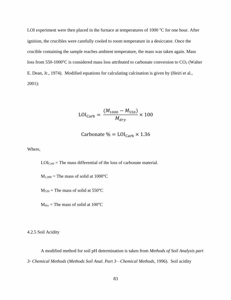
83

LOI experiment were then placed in the furnace at temperatures of 1000 °C for one hour. After

ignition, the crucibles were carefully cooled to room temperature in a desiccator. Once the

crucible containing the sample reaches ambient temperature, the mass was taken again. Mass

loss from 550-1000°C is considered mass loss attributed to carbonate conversion to CO2 (Walter

E. Dean, Jr., 1974). Modified equations for calculating calcination is given by (Heiri et al.,

2001):

LOICarb = (𝑀1000 − 𝑀550)

𝑀𝑑𝑟𝑦× 100

Carbonate % = LOICarb × 1.36

Where,

LOICarb = The mass differential of the loss of carbonate material.

M1,000 = The mass of solid at 1000°C

M550 = The mass of solid at 550°C

Mdry = The mass of solid at 100°C

4.2.5 Soil Acidity

A modified method for soil pH determination is taken from Methods of Soil Analysis part

3- Chemical Methods (Methods Soil Anal. Part 3—Chemical Methods, 1996). Soil acidity

84

analysis determines pH using a 1M KCL solution. 2 g of sample, from each sampled depth, was

massed out and placed in a 15ml centrifuge tube. 2 ml of 1M KCL was added to the sample and

mixed. The mixture was rested for ten-minutes then measured with a Mettler Toledo Five Easy

Plus meter and pH probe. The pH is recorded as pHKCl (Methods Soil Anal. Part 3—Chemical

Methods, 1996).

4.2.6 Heavy Acid Digestion

Small-sized particles (850 µM, 600 µM, 425 µM, 300 µM, 180 µM, 150 µM, 75 µM,

<75 µM) were subsampled for heavy digestion analysis. Each particle subset was massed in 30

mL PFA vials. Reverse aqua regia was determined as the most appropriate method for digestion.

The method involved using three-parts concentrated nitric acid with one-part hydrochloric acid.

Digestion was performed until dryness and repeated in triplicate. Digested sediment is pickup in

10 mL of a known amount of 5% HNO3. The 5% supernatant was siphoned off from teflon tubes

into a plastic centrifuge tube and used as sample stock. Dilutions are sampled from the sample

stock and prepared for elemental analysis. All acids used were ACS grade concentrated mineral

acids from Fisher Chemical.

4.2.7 Elemental Analysis

A methodology used for sediment metal concentration determination via inductively

coupled plasma mass spectrometry (ICP-MS) was taken from Al-Mur et al. (2017). Briefly, the

method involved used a 5% HNO3 matrix, prepared from trace metal grade concentrated 65-70%

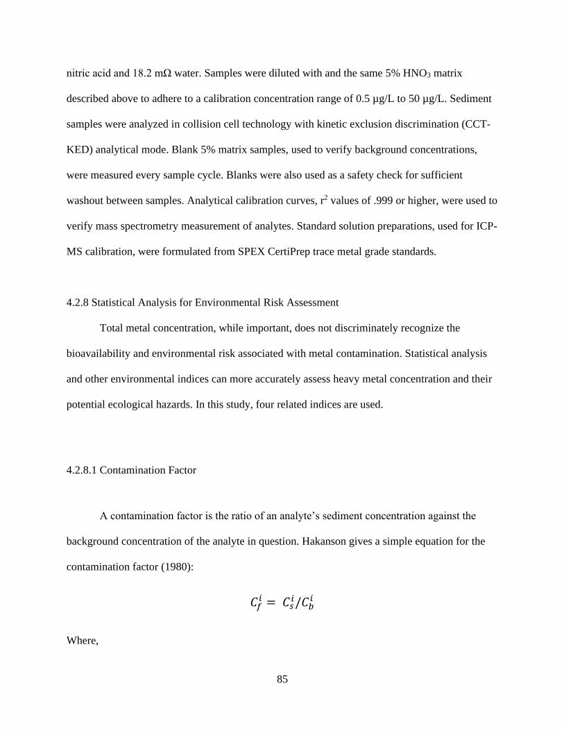
85

nitric acid and 18.2 mΩ water. Samples were diluted with and the same 5% HNO3 matrix

described above to adhere to a calibration concentration range of 0.5 µg/L to 50 µg/L. Sediment

samples were analyzed in collision cell technology with kinetic exclusion discrimination (CCT-

KED) analytical mode. Blank 5% matrix samples, used to verify background concentrations,

were measured every sample cycle. Blanks were also used as a safety check for sufficient

washout between samples. Analytical calibration curves, r2 values of .999 or higher, were used to

verify mass spectrometry measurement of analytes. Standard solution preparations, used for ICP-

MS calibration, were formulated from SPEX CertiPrep trace metal grade standards.

4.2.8 Statistical Analysis for Environmental Risk Assessment

Total metal concentration, while important, does not discriminately recognize the

bioavailability and environmental risk associated with metal contamination. Statistical analysis

and other environmental indices can more accurately assess heavy metal concentration and their

potential ecological hazards. In this study, four related indices are used.

4.2.8.1 Contamination Factor

A contamination factor is the ratio of an analyte’s sediment concentration against the

background concentration of the analyte in question. Hakanson gives a simple equation for the

contamination factor (1980):

𝐶𝑓𝑖 = 𝐶𝑠

𝑖/𝐶𝑏𝑖

Where,

86

Csi = the concentration of the specific metal

Cbi = the background value for the metal in question

Background values are metal-specific, and are described by Turekian and Wedepohl,

1961. For this study, Cbi are sedimentary mg/kg values where: V=130, Cr=90, Mn=850, Ni =68,

Cu =45, Zn=95, Mo= 2.6, Cd=0.3, Pb=20, and U= 3.7. Terminology, from Hakanson, is used to

qualify and categorize calculated Cfi values. A contamination factor <1equates to low

contamination of the sediment. 1≤Cfi<3 refers to a moderate contaminated sediment. When 3

≥Cfi <6 is a considerably contaminated sediment, and when Cf

i ≥6 is a very high contamination

factor for a given element (1980).

4.2.8.2 Pollution Load Index (PLI)

The Pollution Load Index gives an overall summation of contamination-weighted

concentrations for all analytes of interest in a given site or sample (Rabee. A, et al., 2011). In this

study, PLI is calculated per particle size for each location to find the total pollution potential a

particular fraction size produces. An equation for determining PLI is given by (Tomlinson et al.,

1980):

Where,

Cf = the contamination factor

n = the number metals used to determine PLI

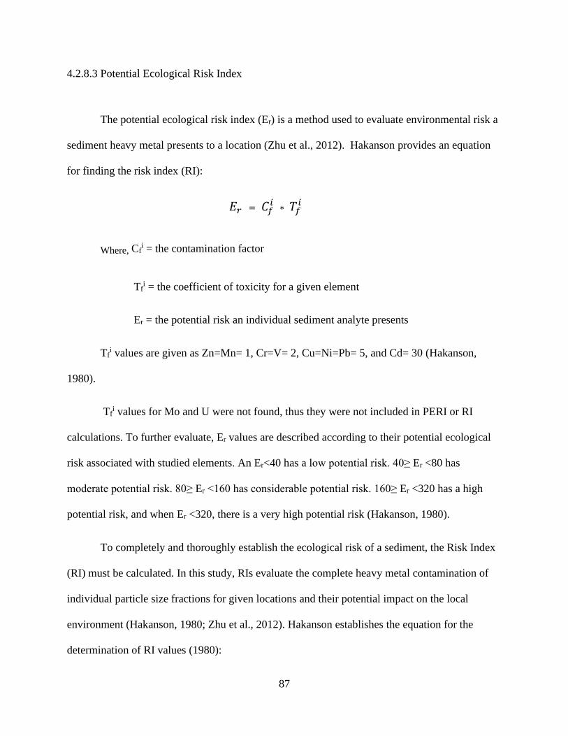
87

4.2.8.3 Potential Ecological Risk Index

The potential ecological risk index (Er) is a method used to evaluate environmental risk a

sediment heavy metal presents to a location (Zhu et al., 2012). Hakanson provides an equation

for finding the risk index (RI):

𝐸𝑟 = 𝐶𝑓𝑖 ∗ 𝑇𝑓

𝑖

Where, Cfi = the contamination factor

Tfi = the coefficient of toxicity for a given element

Er = the potential risk an individual sediment analyte presents

Tfi values are given as Zn=Mn= 1, Cr=V= 2, Cu=Ni=Pb= 5, and Cd= 30 (Hakanson,

1980).

Tfi values for Mo and U were not found, thus they were not included in PERI or RI

calculations. To further evaluate, Er values are described according to their potential ecological

risk associated with studied elements. An Er<40 has a low potential risk. 40≥ Er <80 has

moderate potential risk. 80≥ Er <160 has considerable potential risk. 160≥ Er <320 has a high

potential risk, and when Er <320, there is a very high potential risk (Hakanson, 1980).

To completely and thoroughly establish the ecological risk of a sediment, the Risk Index

(RI) must be calculated. In this study, RIs evaluate the complete heavy metal contamination of

individual particle size fractions for given locations and their potential impact on the local

environment (Hakanson, 1980; Zhu et al., 2012). Hakanson establishes the equation for the

determination of RI values (1980):

88

𝑅𝐼 = ∑ 𝐸𝑟

Where, the risk index (RI) is the sum of the ecological risk by individual metals.

Given categories for RI values are as follows: RI <150 equates to a low risk; 150≥RI<300 leads

to a moderate risk; 300≥RI <600 is a considerable risk; RI ≥600 is a very high-risk factor.

4.3 Results

Particle size distribution was investigated near-surface sediment of collected grab

samples, representing two different sites of interest. Samples were collected from sites

previously verified for high concentrations of transition and heavy metals, including Mn, U, V,

and Cr. Size fractionation of near-surface sediment, of samples collected from the marshland, is

shown in Figures 4.1 & 4.2. There is not a noticeably large discrepancy of particle fractionation

between samples A & B. Both samples mimic each other in terms of size distribution.

Specifically, particulate masses of both samples are concentrated in the larger fractions, mostly

sizes of 4.75mm and 2.76mm, with minor amounts in the smaller fractions (Figures 4.1 & 4.2).

Figures 4.3 & 4.4 present the size distribution data of near-surface particles sampled at

site BG2-4. While sampled identically and simultaneously, fractionation from sample A to B

differs enormously (Figures 4.3 & 4.4). Sample A is shown to have ample of mass in nearly all

size fractions, with large mass percentages in the fine fractions of 300µm and 180µm (Figure

4.3). Sample B exhibits a far different fractionation. Particle mass, from sample B, is

concentrated in the 180µm and 300µm fraction sizes (Figure 4.4). Discrepancy between the two

samples is attributed to field variance within the BG2-4 sampling location.

89

Following size fractionation, soil acidity was tested on all four samples separately. Figure

4.5 describes the soil acidity of each sample for fractionation sizes down to 75µm. pH testing

indicated that there is a high degree of pH variability between the two sampled locations.

Variance amongst A & B samples is near-constant for samples coming from location BG2-4. A

pH unit difference is observed between samples A & B regardless of particle size. Samples from

location BG2-3 display low pH variance across all particle sizes, however, smaller particle sizes

do exhibit larger pH changes between samples A & B.

Elemental analysis is the starting point for determining ecological risk. Metal concentrations are

determined per particle size for all four samples. For both site locations, the average

concentrations for heavy metal analysis of the two samples is presented and used for multiple

ecological indices (Table 4.1). Particle contamination factors (Cfi) for V, Cr, Mn, Ni, Cu, Zn,

Mo, Cd, Pb, and U are presented in Table 4. 2.

Contamination factors quantify the degree of toxicity an element or substance has on its

environment. From Table 4.3, elemental contamination factors vary greatly in their pollution of

sediment fractions. However, small fractions below 75µm exhibit higher contamination than

other sizes. This is seen in both average fraction sets. Cd exhibits the highest contamination risk,

independent of particle size and site location, with a very high contamination factor. Other

analytes, Mo and U both express contamination factors with moderate to considerable

contamination, depending on fraction size. Low contamination is exhibited on the fraction by

many of the metals studied; however, even among the metals exhibiting a low contamination, the

sub 75µm fraction is relatively elevated.

90

The average pollution load index (PLI) of each fraction is given in Figure 4.7. The PLIs,

are determined by the equation from Tomlinson (1980). Across both sites, the highest average

PLI of each average sample was the sub 75µm fraction size. This confirms pollution potential

levels to be size-dependent.

Table 4.3 presents the potential ecological risk factor (Er) for individual heavy metals

at the particulate sizes examined. Er is described as the potential risk of an individual metal at a

certain location (Zhu et al., 2012). Hakanson similarly classifies Ers to the previous

contamination factors. Most of the Er values present low ecological risk. Cu, at sub75 µm for

Site1, does show a moderate ecological risk. On average, the heavy metals studied present higher

Er values at sub 75 µm even though they are considered low risk.

Figure 4.8 illustrates the average calculated Risk Index (RI) for each fraction size at each

location. The RIs calculated here are the sum of each metal’s ecological risk for a given fraction

size. Using the defined terminology from Hakanson, RIs record low ecological risk; however,

sub 75µm fractions still present a higher ecological risk over larger particle sizes.

4.4 Discussion

Soil particle size distribution amongst the respective samples, is not ubiquitous at each

site location. Figures 4.1-4.4 detail the particle distribution differences between each sample.

Figures 4.1 & 4.2 show that samples A & B, collected from Site1, show similarities in their

distributions. However, Figures 4.3 & 4.4 reveal significant differences between samples A & B

collected from Site2. It is understandable to see a difference between the samples from one site

to the other. Topography of Site1 differs from Site2. Site1 being a lowland swampy region and

91

Site2 a hilly region with a looser and rockier sediment profile. The large distinction between

Site2’s A & B samples is related to regional in situ field variance. Sediment profiles from this

region vary in terms of particle size distribution as well as organic material, and soil acidity.

The soil acidity profile details similar pH distinctions between particle distributions and

site locations. There is a larger pH discrepancy between Site2’s A & B samples versus the

samples taken from Site1; however, there is no differential pH trend between distribution and

particle size. The soil pH has a strong influence on metal concentrations and helps to explain

why metal concentrations are higher at Site1 versus Site2.

Soil pH only presents a partial answer to metal concentrations and the association with

particle size. It has been well documented that small particle sizes have an affinity for metal

sorption (Hamilton-Taylor et al., 1997; Nnaji and Emefu, 2017). As observed, particle sizes

under 75 µm have a higher metal concentration. While soil pH is a factor in this phenomenon, it

is mainly due to the increased soil organic matter in these fraction sizes. Figure 6 contrasts the

organic and carbonate material present in bulk versus sub 75µm particles. Organic material is

more abundant in the subfractions than the bulk material, especially Site1’s B sample. Organic

matter in this fraction is substantial and provides rationale, along with observed acidic pH values,

as to why metal concentrations are higher in this fraction than any other. It is well documented

that organic material sequesters many metals (Schijf and Zoll, 2011; Wen et al., 1997).

Furthermore, the metals found to be elevated on sub 75µm particles are commonly, and strongly

bound to organic material (Weng et al., 2002). With the available organic matter and pH

conditions, sub 75µm particles are suitable for fostering high metal concentrations.

92

While small particle sizes do hold higher metal concentrations, that does not necessarily

mean they present an environmental or ecological risk. Ecological risk is assessed on particle

distributions and evaluated for their ecological impact. Particle distributions are first evaluated

for their contamination factors (Cfi). Cf

i values are categorized according to terminology

developed by Hakanson (1980). From Table 4.2 it is observed that the Cfi for most of the

elements presents low contamination of the sediment, with the highest contamination factors

nominally being distributed on fine size particles. Uranium (U) is evaluated for having moderate

soil contamination in most distributions, while Molybdenum (Mo) expresses considerable

contamination in every distribution from Site1. Mo is evaluated for moderate contamination

amongst all distributions in Site2. Copper (Cu) presents the highest contamination factor for fine-

sized particles.

The PLI indicates a similar trend of fine size particles containing higher levels of

pollution than larger masses. However, this trend is observed most noticeably on particles

obtained from Site1. While the trend holds for particles from Site2, the pollution differential does

not indicate a severe difference in particle size. PLI not only illustrates the pollution levels over

particle distributions but also from the variance per site. PLI confirms that larger particles and

sub 75 µm particles, from Site2, are consistent with natural metal abundance. All PLI’s for these

particles fall under a value of 0.5. However, the fine fractions related to Site1 show a PLI greater

than 1. A PLI greater than 1 indicates contamination within the local area. Whether that is natural

or anthropogenic is yet unknown within the scope of this study.

Er and RI values demonstrate that particle size does factor into available ecological risk,

at both site locations. Cu and Pb are the dominant hazards in small particle sizes. At Site1, Cu on

sub 75µm is given as a moderate potential risk while Pb, though elevated, is seen as low

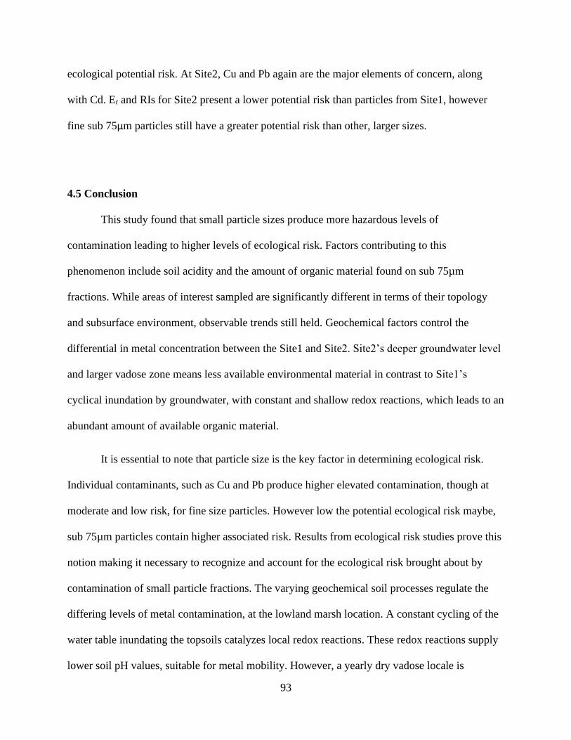
93

ecological potential risk. At Site2, Cu and Pb again are the major elements of concern, along

with Cd. Er and RIs for Site2 present a lower potential risk than particles from Site1, however

fine sub 75µm particles still have a greater potential risk than other, larger sizes.

4.5 Conclusion

This study found that small particle sizes produce more hazardous levels of

contamination leading to higher levels of ecological risk. Factors contributing to this

phenomenon include soil acidity and the amount of organic material found on sub 75µm

fractions. While areas of interest sampled are significantly different in terms of their topology

and subsurface environment, observable trends still held. Geochemical factors control the

differential in metal concentration between the Site1 and Site2. Site2’s deeper groundwater level

and larger vadose zone means less available environmental material in contrast to Site1’s

cyclical inundation by groundwater, with constant and shallow redox reactions, which leads to an

abundant amount of available organic material.

It is essential to note that particle size is the key factor in determining ecological risk.

Individual contaminants, such as Cu and Pb produce higher elevated contamination, though at

moderate and low risk, for fine size particles. However low the potential ecological risk maybe,

sub 75µm particles contain higher associated risk. Results from ecological risk studies prove this

notion making it necessary to recognize and account for the ecological risk brought about by

contamination of small particle fractions. The varying geochemical soil processes regulate the

differing levels of metal contamination, at the lowland marsh location. A constant cycling of the

water table inundating the topsoils catalyzes local redox reactions. These redox reactions supply

lower soil pH values, suitable for metal mobility. However, a yearly dry vadose locale is

94

constantly oxidized. The locale may be subjected to harsher weathering, on the topsoil, resulting

in a larger number of finer particles, including sub 75 µm as supported by Figures 1-4. However,

the oxidized environment does not promote the subsurface conditions allowing for major metal

mobility.

Ultimately, this study looks at most likely naturally occurring toxic metals. Thorough

investigation of both sites indicate subsurface processes encouraging higher metal concentrations

at Site1 versus Site2. While this investigation centered on naturally occurring metals, there are

indications of potential anthropogenic toxicity as well. The PLI values, Figure 4.7, suggest

anthropogenic pollution is affecting Bugesera heterogeneously. Lead abundances most heavily

contribute to PLI values for all particle sizes at both locales. The PLI expression, therefore,

suggests anthropogenic lead likely from an atmospheric source. Further studies can verify this

claim and further determine the sourcing of Pb. All these findings play into the safety and public

health of current populations in the region. Future development in the region should also note the

potential risk of mobilization of not just dust fractions but the heavy metal load therein.

95

4.6 Figures & Tables

Figure 4. 1) Site1 A’s Particle Size Distribution. The top panel illustrates the mass of particle

sizes in descending order. The left y-axis shows each size distribution’s percentage of the total

sampled mass.X-axis displays particle size distribution. The bottom chart illustrates the mass

percent of each particle distribution in descending size order.

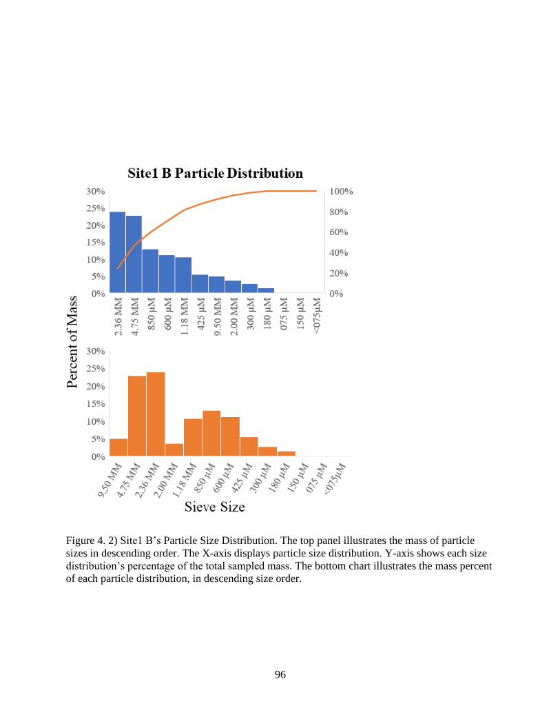
96

Figure 4. 2) Site1 B’s Particle Size Distribution. The top panel illustrates the mass of particle

sizes in descending order. The X-axis displays particle size distribution. Y-axis shows each size

distribution’s percentage of the total sampled mass. The bottom chart illustrates the mass percent

of each particle distribution, in descending size order.

97

Figure 4. 3) Site2 A’s Particle Size Distribution. The top panel illustrates the mass of particle

sizes in descending order. The left y-axis shows each size distribution’s percentage of the total

sampled mass. The X-axis displays particle size distribution. The bottom chart illustrates the

mass percent of each particle distribution, in descending size order.

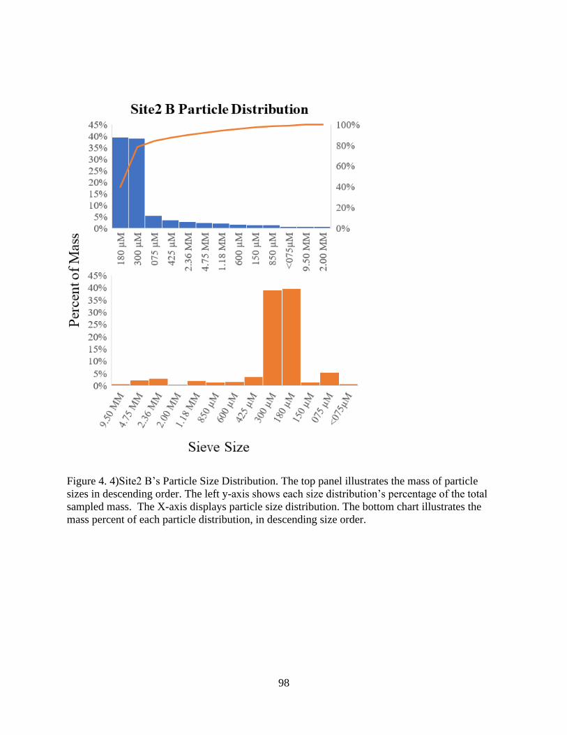
98

Figure 4. 4)Site2 B’s Particle Size Distribution. The top panel illustrates the mass of particle

sizes in descending order. The left y-axis shows each size distribution’s percentage of the total

sampled mass. The X-axis displays particle size distribution. The bottom chart illustrates the

mass percent of each particle distribution, in descending size order.

99

Figure 4. 5) Soil Acidity for Sites1 & 2. The average pHkcl values of each particle size from Site1

and Site2. The more acidic green bars indicate soil pH at Site1. Site2 soil pH values, shown in

blue, are near circumneutral levels.

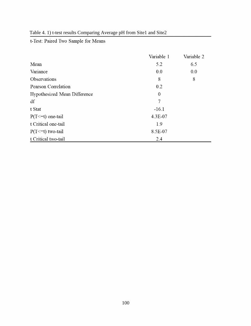
100

Table 4. 1) t-test results Comparing Average pH from Site1 and Site2

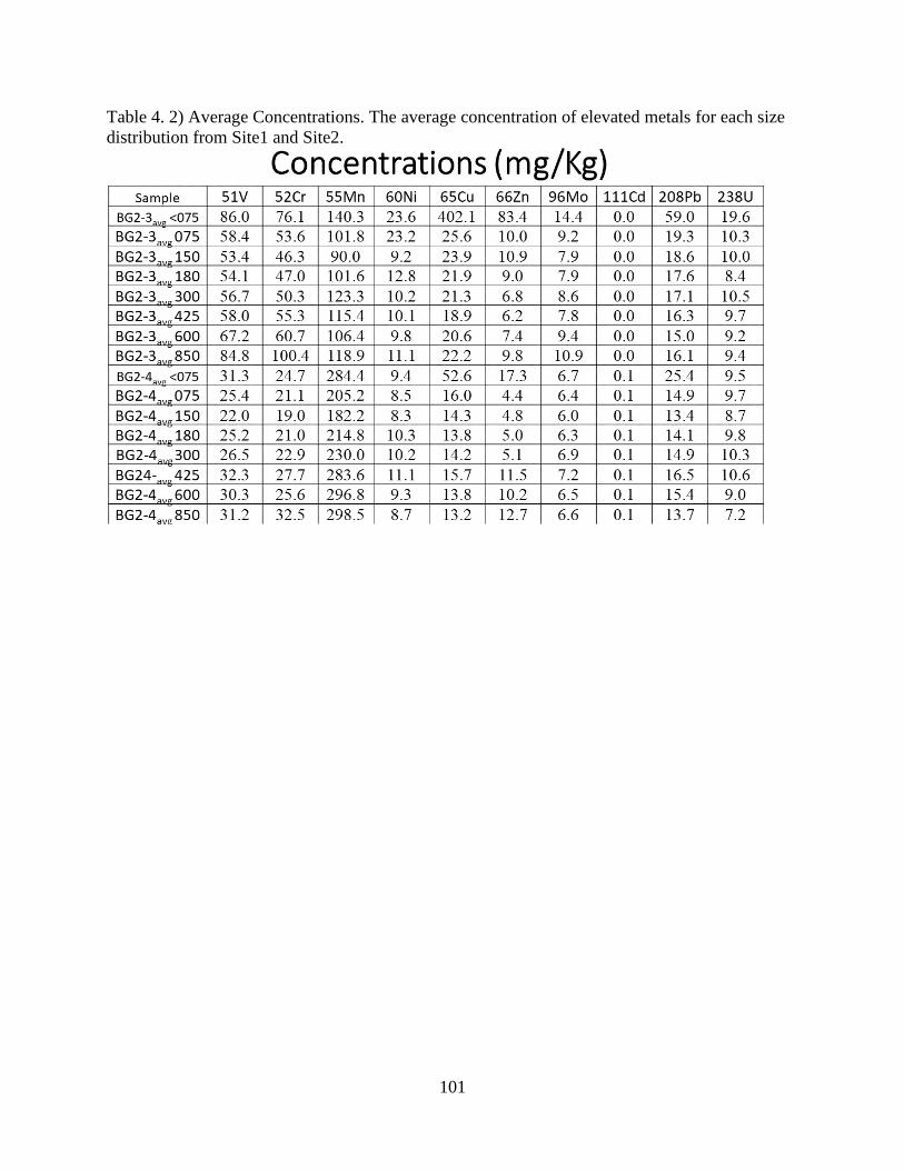
101

Table 4. 2) Average Concentrations. The average concentration of elevated metals for each size

distribution from Site1 and Site2.

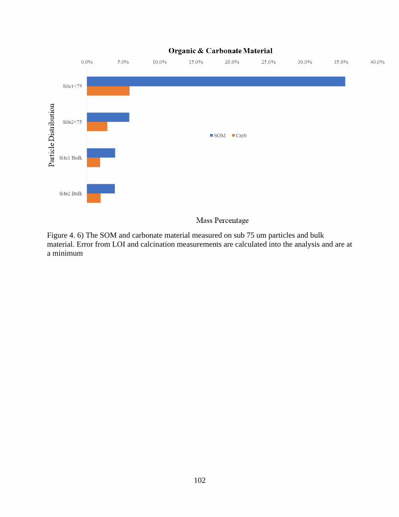
102

Figure 4. 6) The SOM and carbonate material measured on sub 75 um particles and bulk

material. Error from LOI and calcination measurements are calculated into the analysis and are at

a minimum

103

Table 4. 3) The average contamination factor, Cf, of measured metals. Cfs are applied to each

particle from both Site1 and Site2.

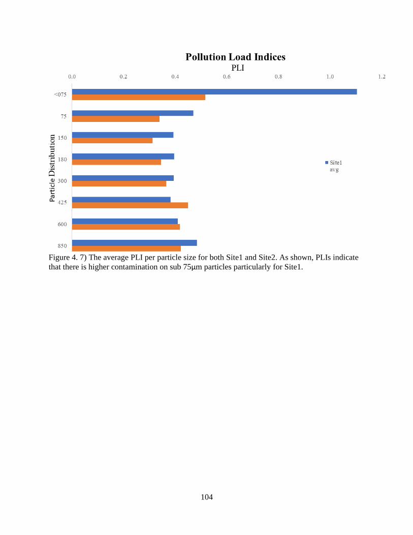
104

Figure 4. 7) The average PLI per particle size for both Site1 and Site2. As shown, PLIs indicate

that there is higher contamination on sub 75µm particles particularly for Site1.

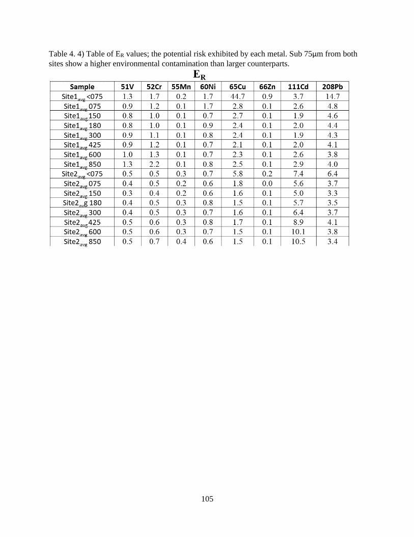
105

Table 4. 4) Table of ER values; the potential risk exhibited by each metal. Sub 75µm from both

sites show a higher environmental contamination than larger counterparts.

106

Figure 4. 8) The Risk Index of each particle size for Site1 and Site2. The Risk Index illustrates

the contamination difference between sub 75µm particles and lager particle masses. Also

illustrated are the differences in contamination between and area with cyclical redox against a

yearly dry vadose zone. Fine particle masses, regardless of site location, poses the greatest threat

to the surrounding environment and the public health.

107

CHAPTER 5

Conclusion

5.1 Summarization

This dissertation demonstrates that understanding the geochemical processes involved

with the release of naturally occurring metals is an essential initial phase for mitigation. Chapter

2 examines Pb contamination in Bangladeshi refugee camp drinking water wells. Naturally

occurring Pb is found to be elevated throughout the Kutupalong settlement. Further examination

of the matter revealed that Pb release was controlled by a series of biogeochemical processes.

Nutrient loading, via fertilization and animal waste, drives nitrogen dynamics causing shifts in

the groundwater pH. The pH swings thus dictate Pb sorption and solubility of Pb containing Fe

and Mn hydroxide particles. Instead of an in situ method for mitigating Pb, risk assessment maps

were designed to manage contamination through avoidance as well as provide strategic planning

for the implementation of future wells and the closure of currently contaminated ones.

Chapter 3 assesses elevated levels of multiple trace and heavy metal contaminants in

near-surface sediments of Bugesera, Rwanda. Three different sites were cored to evaluate Mn, U,

and V in subsurface sediment. Sequential extractions determined the speciation of subsurface

metal contaminants. Phase determination, in combination with soil acidity, LOI, and calcination

measurements yielded an evaluation of the mobility and potential bioavailability of Mn, U, and

V. This study ultimately contrasts locales with cyclical redox changes, due to groundwater

oscillation, to a yearly vadose region. Different mechanisms of potential metal release were

identified at each site. The specific locale within Bugesera will often dictate the geochemical

processes associated with metal release. Ideally, understanding many of these complex

108

geochemical processes should be used to help further the subsurface awareness of contamination

risk in Bugesera. Thus, allowing for safe, sustainable growth in the region.

Chapter 4 of this dissertation investigates potential airborne contamination of fine size

dust particles in Bugesera. Surface particle size distribution was measured and evaluated for

trace and heavy metals. Though complete elemental breakdown is assessed, it alone is

inadequate to determine total hazardous potential dust particles pose on the surrounding

environment. Ecological risk indices were applied to establish environmental risk. Risk indices

determine that the highest level of risk came from Site1, with Cu and Pb presenting the greatest

risk. The highest risk assessment from Site2 was found to come from Pb, Cd, and Cu

contamination. As asserted, particle size does influence the risk level in calculated ecological

indices. However, Cd ecological risk is noticeably higher on larger particle sizes at site2. While

Cd does not change the ecological trend of smaller particle sizes producing higher risk, it is

worth noting that there is a higher ecological risk for Cd among larger particles. From the

independently calculated RIs, it is determined that while ecological risk is low, there is a larger

risk with fine particles, especially from Site1.

This dissertation examines mechanisms for trace and heavy metal release, chiefly through

the soil-water interface of tropical soil profiles. The findings from this dissertation attain to

emphasize the vulnerability of communities, in these two regions, to metal contamination

exposure. In Bangladesh, the uses of risk assessment maps as a mitigation technique that is used

for current and potential contamination avoidance. The use of risk maps, in Kutupalong, is a way

to avoid Pb contaminated and potentially contaminated areas. Also, they are to be used in

strategic development and site planning, for the influx of future settlement inhabitants. Risk

maps apply to every world region, provided adequate data has been collected. Using a GIS tool

109

for mapping purposes is a cost-effective and ecologically conservative method for mitigating

risk. Globally, there are numerous different functions for risk maps and assessments. While the

maps provided in this dissertation do not directly correlate to any other region beyond their

intended use, variations and multilayer GIS maps dedicated to specific locations can provide an

accurate assessment of ecological exposure and public health risk.

Chapters 3 and 4 present assessments rather than outlined mitigation strategies. These

evaluations apply to other parts of the world. Sampling was completed in the East African Rift

Valley. It is reasonable to presume that similar geochemical processes take place in other rift

valleys, especially in the global south with similar tropical soil profiles.

Findings from chapters 3 and 4 from this dissertation may not layout concrete planning of

mitigation or remediation. However, results do indicate that extensive care should be placed in

the Bugesera region during development. Rwanda is in the process of developing Bugesera,

including the construction of the country’s largest international airport. If consideration is not

taken during development, it is quite plausible for the community to be susceptible to high-risk

exposure. Subsurface contamination and inhalation are factors that contribute to environmental

exposure and public health risk.

Part of engineering is gathering all available data to make the most informed decision

possible. Data collection is never truly complete as more can always be collected and processed,

as is the case for this dissertation. Further study of the spatial extent of geochemical processes at

each studied locale would build an extensive foundation in each location’s subsurface chemistry

in conjunction with comprehensive depth modeling. Building a near-complete model of the

region’s subsurface geochemistry and the local geochemical processes will greatly help in the

ecological and environmental development aspects of Bugesera. Furthermore, initiating a

110

geologic control study would help to compare sediment on granite bedrock in Bugesera to that of

shale bedrock found in other Rwandan regions. This should show the variance in naturally

occurring metals and indicate the differing soil expression across contrasting Rwandan regions.

In addition to previously sampled sub 75µm particles, it would be beneficial to further

fractionate these masses into soil particulates of PM10 and PM2.5. The current sub 75µm mass is a

combination of fine size and particulate matter including PM10 and PM2.5. Analysis of

particulate matter falling into these two fractions will further demonstrate the hazards presented

by airborne particles. These two particle sizes alone can be considered carcinogenic (Kim et al.,

2019). Collecting PM10 and PM2.5 would allow for in-depth dispersion modeling. Using the

climatic setting of Bugesera and considering the source of PM being highly weathered

sediments, a dispersion model can identify the extent of PM travel. As different particle sizes

travel at different rates, the model would identify locations where expected PM fractions would

be expected to cluster.

Continued elemental analysis on different particles would advantageously increase the

understanding of potential risk association. Sequential extraction experiments, applied to fine

particle sizes, will further determine the speciation of trace and heavy metals. Knowing phase or

speciation is a key component in assessing public health risk. Phase will help determine potential

environmental release and potential bioavailability. Finally, adding Pb isotope analysis, and

combining it with elemental regressions will be able to source Pb and, indirectly, other major

associated contaminants. The ultimate culmination of the techniques from this dissertation

would use a multi-layered GIS map, consisting of multiple analytes paired with corresponding

toxicity factors, to appropriately weight mapping algorithms. Risk maps applied to the water

quality problem found in Kutupalong are unique. They were also the recommended solution

111

provided to the UNHCR as a mitigation strategy to the Pb issues in Kutupalong. This strategy

helps the UNHCR and settlement leaders solve their drinking water issue without the economic

and environmental strains of implementing a massive project. Combining and pairing these

techniques will create a map illustrating the regional scale of toxic metal risk providing a useful

regional tool like the small-scale tool constructed in the Kutapalong refugee settlement.

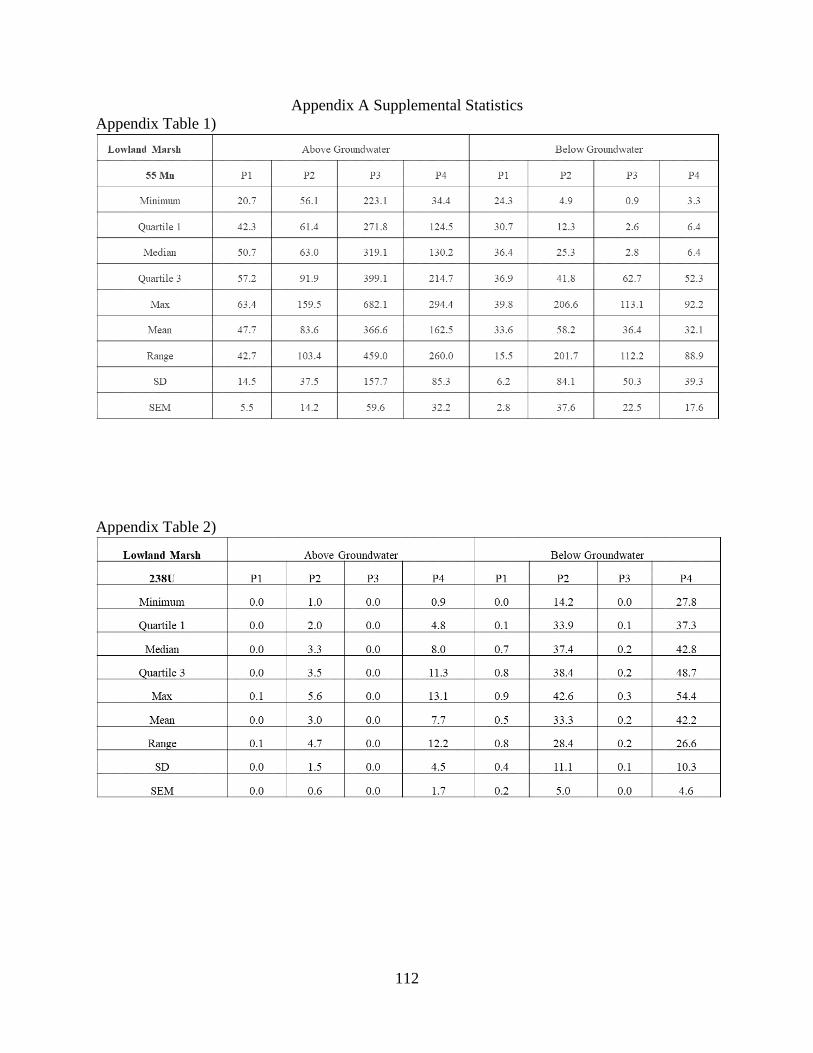
112

Appendix A Supplemental Statistics

Appendix Table 1)

Appendix Table 2)

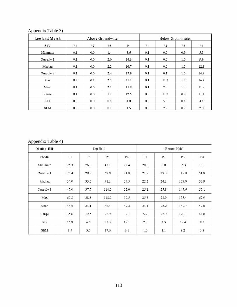
113

Appendix Table 3)

Appendix Table 4)

114

Appendix Table 5)

Appendix Table 6)

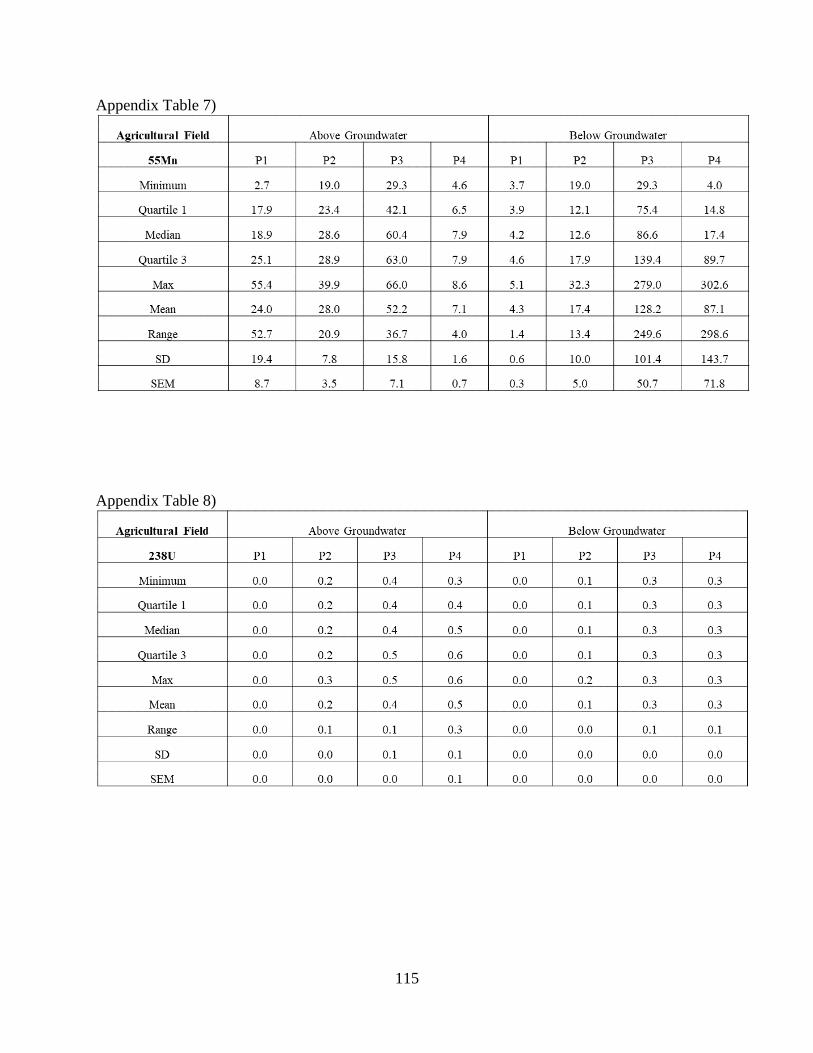
115

Appendix Table 7)

Appendix Table 8)

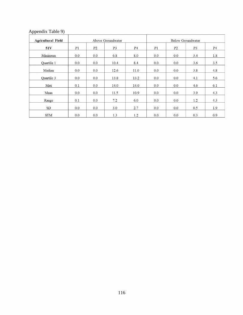
116

Appendix Table 9)

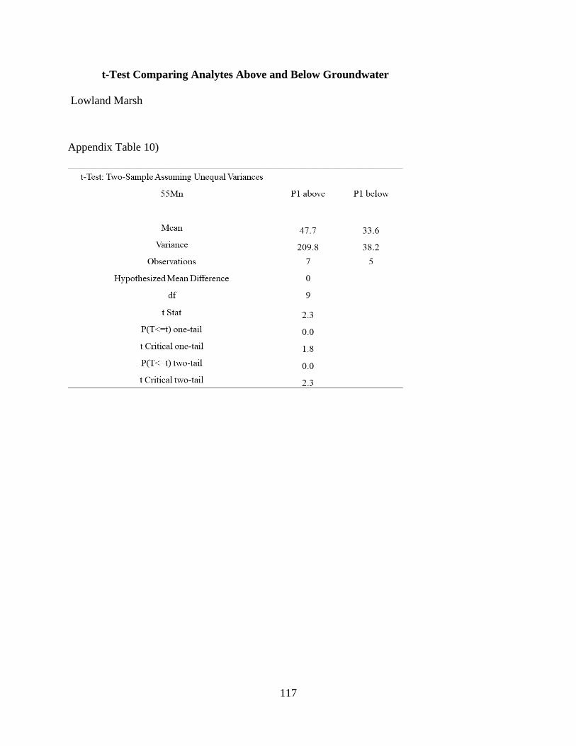
117

t-Test Comparing Analytes Above and Below Groundwater

Lowland Marsh

Appendix Table 10)

118

Appendix Table 11)

Appendix Table 12)

119

Appendix Table 13)

Appendix Table 14)

120

Appendix Table 15)

Appendix Table 16)

121

Appendix Table 17)

Appendix Table 18)

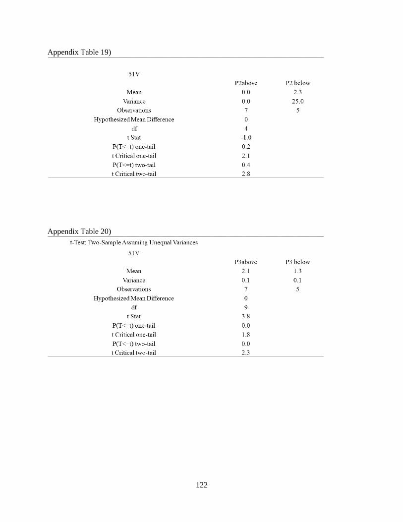
122

Appendix Table 19)

Appendix Table 20)

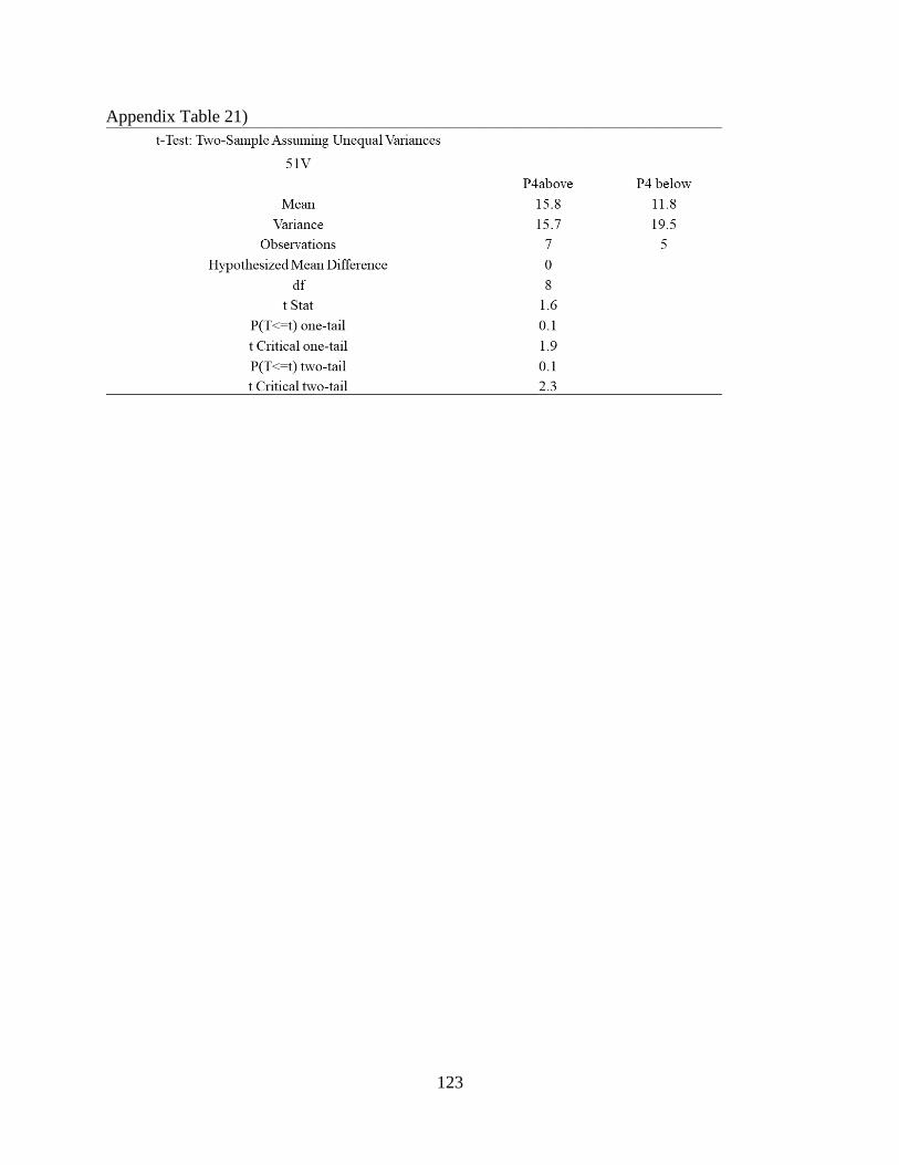
123

Appendix Table 21)

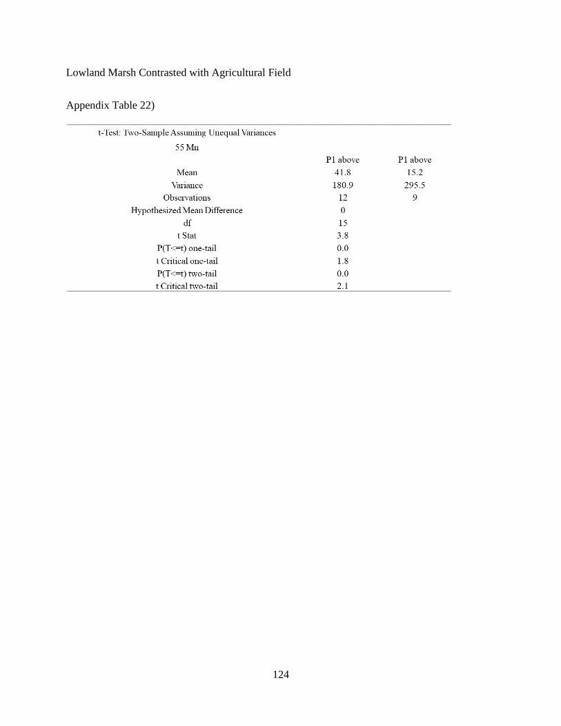
124

Lowland Marsh Contrasted with Agricultural Field

Appendix Table 22)

125

Appendix Table 23)

Appendix Table 24)

126

Appendix Table 25)

Appendix Table 26)

127

Appendix Table 27)

Appendix Table 28)

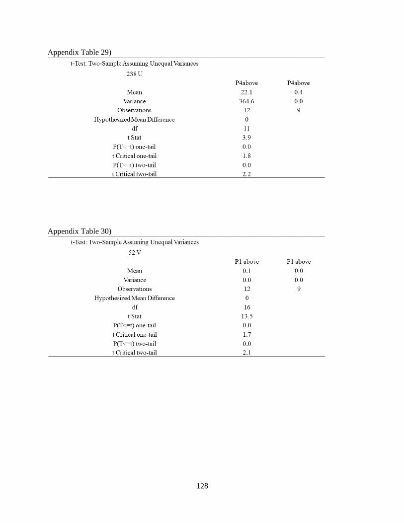
128

Appendix Table 29)

Appendix Table 30)

129

Appendix Table 31)

Appendix Table 32)

130

Appendix Table 33)

131

Works by Kenneth Hamilton II

Hamilton, KM*; Wilson, ME*; Grant, KE*; Aleto, DM*; Quicksall, AN. Groundwater Lead and

Nitrate Mapping for Origination and Risk Assessment in Kutupalong, Bangladesh. Water

Research. (Under Review).

Hamilton, KH*; Quicksall, AN. Inherent Toxicity Through Dispersion of Sized Determined Dust

Particles in Bugesera, Rwanda.

Hamilton, KH*; Quicksall, AN. Spatial Resolution and Origination of Toxic elements in the

Soil-Water Partitioning of Subsurface Bugesera (Working).

Bayan, MA*; Hamilton, KM*; Quicksall, AN. Lab Scale Assessment of Biological Filtration for

Removal of Microconstituents in Drinking Water. ACS 2014.

Hamilton, KM*; Wilson, ME*; Aleto, DM*; Grant, KE*; Quicksall, AN. Mapping of

Contaminants in Developing World Aquifers for Origination and Risk Assessment. OU Water

Conference 2015

132

BIBLIOGRAPHY

Al-Mur, B.A., Quicksall, A.N., Al-Ansari, A.M.A., 2017. Spatial and temporal distribution of

heavy metals in coastal core sediments from the Red Sea, Saudi Arabia. Oceanologia.

https://doi.org/10.1016/j.oceano.2017.03.003

Bajwa, B.S., Kumar, S., Singh, S., Sahoo, S.K., Tripathi, R.M., 2017. Uranium and other heavy

toxic elements distribution in the drinking water samples of SW-Punjab, India. J. Radiat.

Res. Appl. Sci. https://doi.org/10.1016/j.jrras.2015.01.002

Bredberg, K., Karlsson, H.T., Holst, O., 2004. Reduction of vanadium(V) with Acidithiobacillus

ferrooxidans and Acidithiobacillus thiooxidans. Bioresour. Technol.

https://doi.org/10.1016/j.biortech.2003.08.004

Brettar, I., Sanchez-Perez, J.M., Trémolières, M., 2002. Nitrate elimination by denitrification in

hardwood forest soils of the Upper Rhine floodplain - Correlation with redox potential and

organic matter. Hydrobiologia 469, 11–21. https://doi.org/10.1023/A:1015527611350

Carpi, A., 1997. Mercury from combustion sources: A review of the chemical species emitted

and their transport in the atmosphere. Water. Air. Soil Pollut.

https://doi.org/10.1007/BF02047037

Carter, R.C., Tyrrel, S.F., Howsam, P., 1996. Strategies for handpump water supply programmes

in less-developed countries. Water Environ. J. 10, 130–136. https://doi.org/10.1111/j.1747-

6593.1996.tb00022.x

Chen, Z.S., Lee, G.J., Liu, J.C., 2000. The effects of chemical remediation treatments on the

extractability and speciation of cadmium and lead in contaminated soils. Chemosphere 41,

133

235–242. https://doi.org/10.1016/S0045-6535(99)00416-6

Crossgrove, J., Zheng, W., 2004. Manganese toxicity upon overexposure. NMR Biomed.

https://doi.org/10.1002/nbm.931

Das, B., Hazarika, P., Saikia, G., Kalita, H., Goswami, D.C., Das, H.B., Dube, S.N., Dutta, R.K.,

2007. Removal of iron from groundwater by ash: A systematic study of a traditional

method. J. Hazard. Mater. 141, 834–841. https://doi.org/10.1016/j.jhazmat.2006.07.052

Dewaele, S., De Clercq, F., Muchez, P., Schneider, J., Burgess, R., Boyce, A., Fernandez

Alonso, M., 2010. Geology of the cassiterite mineralisation in the Rutongo area, Rwanda

(Central Africa): Current state of knowledge. Geol. Belgica.

Domingo, J.L., 2001. Reproductive and developmental toxicity of natural and depleted uranium:

A review. Reprod. Toxicol. https://doi.org/10.1016/S0890-6238(01)00181-2

Dong, D., Derry, L.A., Lion, L.W., 2003. Pb scavenging from a freshwater lake by Mn oxides in

heterogeneous surface coating materials. Water Res. 37, 1662–1666.

Drever, J.I., 2002. The Geochemistry of Natural Waters, Third. ed. Prentice Hall, Upper saddle

River.

Fan, A.M., Willhite, C.C., Book, S.A., 1987. Evaluation of the nitrate drinking water standard

with reference to infant methemoglobinemia and potential reproductive toxicity. Regul.

Toxicol. Pharmacol. 7, 135–148. https://doi.org/10.1016/0273-2300(87)90024-9

Flora, G., Gupta, D., Tiwari, A., 2012. Toxicity of lead: A review with recent updates.

Interdiscip. Toxicol. https://doi.org/10.2478/v10102-012-0009-2

Frisbie, S.H., Mitchell, E.J., Dustin, H., Maynard, D.M., Sarkar, B., 2012. World health

134

organization discontinues its drinking-water guideline for manganese. Environ. Health

Perspect. https://doi.org/10.1289/ehp.1104693

Gadde, R.R., Laitinen, H.A., 1974. Heavy metal adsorption by hydrous iron and manganese

oxides. Anal. Chem. 46, 2022–2026. https://doi.org/10.1021/ac60349a004

Ghehi, N.G., Nemes, A., Verdoodt, A., Van Ranst, E., Cornelis, W.M., Boeckx, P., 2012.

Nonparametric Techniques for Predicting Soil Bulk Density of Tropical Rainforest Topsoils

in Rwanda. Soil Sci. Soc. Am. J. https://doi.org/10.2136/sssaj2011.0330

Gidlow, D.A., 2004. Lead toxicity. Occup. Med. (Lond). 65, 348–56.

https://doi.org/10.1093/occmed/kqv018

Guagliardi, I., Cicchella, D., De Rosa, R., Ricca, N., Buttafuoco, G., 2018. Geochemical sources

of vanadium in soils: Evidences in a southern Italy area. J. Geochemical Explor.

https://doi.org/10.1016/j.gexplo.2016.11.017

Hakanson, L., 1980. An ecological risk index for aquatic pollution control.a sedimentological

approach. Water Res. https://doi.org/10.1016/0043-1354(80)90143-8

Hamilton-Taylor, J., Giusti, L., Davison, W., Tych, W., Hewitt, C.N., 1997. Sorption of trace

metals (Cu, Pb, Zn) by suspended lake particles in artificial (0.005 M NaNO3) and natural

(Esthwaite Water) freshwaters. Colloids Surfaces A Physicochem. Eng. Asp.

https://doi.org/10.1016/S0927-7757(96)03722-3

Heiri, O., Lotter, A.F., Lemcke, G., 2001. Loss on ignition as a method for estimating organic

and carbonate content in sediments: Reproducibility and comparability of results. J.

Paleolimnol. https://doi.org/10.1023/A:1008119611481

135

HEM, J., 1972. Chemical Factors that Influence the Availability of Iron and Manganese in

Aqueous Systems. Geol. Soc. Am. Bull. 83, 443–450. https://doi.org/10.1130/0016-

7606(1972)83[443:cftita]2.0.co;2

Herndon, E.M., Havig, J.R., Singer, D.M., McCormick, M.L., Kump, L.R., 2018. Manganese

and iron geochemistry in sediments underlying the redox-stratified Fayetteville Green Lake.

Geochim. Cosmochim. Acta. https://doi.org/10.1016/j.gca.2018.04.013

Hosoi, M., Sharhan, D. Al, 2018. Operational Update Bangladesh.

Huang, J.H., Huang, F., Evans, L., Glasauer, S., 2015. Vanadium: Global (bio)geochemistry.

Chem. Geol. https://doi.org/10.1016/j.chemgeo.2015.09.019

Huerta-Diaz, M.A., Tessier, A., Carignan, R., 1998. Geochemistry of trace metals associated

with reduced sulfur in freshwater sediments. Appl. Geochemistry 13, 213–233.

https://doi.org/10.1016/S0883-2927(97)00060-7

Imtiaz, M., Rizwan, M.S., Xiong, S., Li, H., Ashraf, M., Shahzad, S.M., Shahzad, M., Rizwan,

M., Tu, S., 2015. Vanadium, recent advancements and research prospects: A review.

Environ. Int. https://doi.org/10.1016/j.envint.2015.03.018

Jean, G.E., Bancroft, G.M., 1986. Heavy metal adsorption by sulphide mineral surfaces.

Geochim. Cosmochim. Acta 50, 1455–1463. https://doi.org/10.1016/0016-7037(86)90319-4

Jiang, X., Lu, W.X., Zhao, H.Q., Yang, Q.C., Yang, Z.P., 2014. Potential ecological risk

assessment and prediction of soil heavy-metal pollution around coal gangue dump. Nat.

Hazards Earth Syst. Sci. https://doi.org/10.5194/nhess-14-1599-2014

Kim, C.S., Wilson, K.M., Rytuba, J.J., 2011. Particle-size dependence on metal(loid)

136

distributions in mine wastes: Implications for water contamination and human exposure.

Appl. Geochemistry. https://doi.org/10.1016/j.apgeochem.2011.01.007

Kim, K., Byun, Y.H., Lee, D., Park, N., 2019. Understanding the global status of particulate

matter with respect to research topics and research networks. Sustain.

https://doi.org/10.3390/su11205594

Kurttio, P., Komulainen, H., Leino, A., Salonen, L., Auvinen, A., Saha, H., 2005. Bone as a

possible target of chemical toxicity of natural uranium in drinking water. Environ. Health

Perspect. https://doi.org/10.1289/ehp.7475

Lanphear, B.P., Hornung, R., Khoury, J., Yolton, K., Baghurst, P., Bellinger, D.C., Canfield,

R.L., Dietrich, K.N., Bornschein, R., Greene, T., Rothenberg, S.J., Needleman, H.L.,

Schnaas, L., Wasserman, G., Graziano, J., Roberts, R., 2005. Low-level environmental lead

exposure and children’s intellectual function: An international pooled analysis. Environ.

Health Perspect. https://doi.org/10.1289/ehp.7688

Larsen, F.J., Schiffer, T.A., Borniquel, S., Sahlin, K., Ekblom, B., Lundberg, J.O., Weitzberg, E.,

2011. Dietary inorganic nitrate improves mitochondrial efficiency in humans. Cell Metab.

https://doi.org/10.1016/j.cmet.2011.01.004

Mason, L.H., Harp, J.P., Han, D.Y., 2014. Pb neurotoxicity: Neuropsychological effects of lead

toxicity. Biomed Res. Int. https://doi.org/10.1155/2014/840547

McBride, M., Sauvé, S., Hendershot, W., 1997. Solubility control of Cu, Zn, Cd and Pb in

contaminated soils. Eur. J. Soil Sci. https://doi.org/10.1111/j.1365-2389.1997.tb00554.x

McCasland, M. (Cornell U., 1985. Nitrate: Health Effects in Drinking Water. Cornell Coop. Ext.

137

https://doi.org/10.1016/j.bmc.2010.05.076

McKenzie, R.M., 1980. The adsorption of lead and other heavy metals on oxides of manganese

and iron. Aust. J. Soil Res. 18, 61–73. https://doi.org/10.1071/SR9800061

McKenzie, R.M., 1978. The effect of two manganese dioxides on the uptake of lead, cobalt,

nickel, copper and zinc by subterranean clover. Aust. J. Soil Res. 16, 209–214.

https://doi.org/10.1071/SR9780209

Methods of Soil Analysis Part 3—Chemical Methods, 1996.

https://doi.org/10.2136/sssabookser5.3

Morse, J.W., Luther, G.W., 1999. Chemical influences on trace metal-sulfide interactions in

anoxic sediments. Geochim. Cosmochim. Acta 63, 3373–3378.

https://doi.org/10.1016/S0016-7037(99)00258-6

Naidu, R., Sumner, M.E., Harter, R.D., 1998. Sorption of heavy metals in strongly weathered

soils: An overview. Environ. Geochem. Health. https://doi.org/10.1023/A:1006519009465

National Toxicology Program, D. of H. and H.S., 2011. Report on Carcinogens, Twelfth Edition

(2011) - Formaldehyde. Rep. Carcinog.

Needleman, H.L., Bellinger, D., 1991. The health effects of low level exposure to lead. Annu.

Rev. Public Health. https://doi.org/10.1146/annurev.pu.02.050181.001425

Nnaji, C.C., Emefu, S.C., 2017. Effect of particle size on the sorption of lead from water by

different species of sawdust: Equilibrium and kinetic study. BioResources.

https://doi.org/10.15376/biores.12.2.4123-4145

Nriagu, J.O., 1992. Toxic metal pollution in Africa. Sci. Total Environ.

138

https://doi.org/10.1016/0048-9697(92)90304-B

O’Reilly, S.E., Hochella, M.F., 2003. Lead sorption efficiencies of natural and synthetic Mn and

Fe-oxides. Geochim. Cosmochim. Acta 67, 4471–4487. https://doi.org/10.1016/S0016-

7037(03)00413-7

Pourret, O., Dia, A., Gruau, G., Davranche, M., Bouhnik-Le Coz, M., 2012. Assessment of

vanadium distribution in shallow groundwaters. Chem. Geol.

https://doi.org/10.1016/j.chemgeo.2011.11.033

Rabee, A.M., Al-Fatlawy, Y.F., Abd, A.-A.-H.N., Nameer, M., 2011. Using Pollution Load

Index (PLI) and Geoaccumulation Index (I-Geo) for the Assessment of Heavy Metals

Pollution in Tigris River Sediment in Baghdad Region. J. Al-Nahrain Univ. Sci.

https://doi.org/10.22401/jnus.14.4.14

Redmon, J.H., Gibson, J.M.D., Woodward, K.P., Aceituno, A.M., Levine, K.E., 2018.

Safeguarding Children’s Health: Time to Enact a Health-Based Standard and

Comprehensive Testing, Mitigation, and Communication Protocol for Lead in Drinking

Water. N. C. Med. J. https://doi.org/10.18043/ncm.79.5.313

Reed, S., Martens, D., 1996. Methods of Soil Analysis Part 3—Chemical Methods. Methods Soil

Anal. Part 3—Chemical Methods. https://doi.org/10.2136/sssabookser5.3.frontmatter

Rehman, K., Fatima, F., Waheed, I., Akash, M.S.H., 2018. Prevalence of exposure of heavy

metals and their impact on health consequences. J. Cell. Biochem.

https://doi.org/10.1002/jcb.26234

Reijonen, I., Metzler, M., Hartikainen, H., 2016. Impact of soil pH and organic matter on the

139

chemical bioavailability of vanadium species: The underlying basis for risk assessment.

Environ. Pollut. https://doi.org/10.1016/j.envpol.2015.12.046

Rieuwerts, J.S., 2007. The mobility and bioavailability of trace metals in tropical soils: A review.

Chem. Speciat. Bioavailab. https://doi.org/10.3184/095422907X211918

Roy, S., Edwards, M.A., 2019. Preventing another lead (Pb) in drinking water crisis: Lessons

from the Washington D.C. and Flint MI contamination events. Curr. Opin. Environ. Sci.

Heal. https://doi.org/10.1016/j.coesh.2018.10.002

Roychoudhury, A.N., Starke, M.F., 2006. Partitioning and mobility of trace metals in the

Blesbokspruit: Impact assessment of dewatering of mine waters in the East Rand, South

Africa. Appl. Geochemistry. https://doi.org/10.1016/j.apgeochem.2006.02.024

Rwanyiziri, G., Rugema, J., 2013. Climate Change Effects on Food Security in Rwanda: Case

Study of Wetland Rice Production in Bugesera District. Rwanda J.

https://doi.org/10.4314/rj.v1i1.

Salazar, G.J.P., Alfaro-De la Torre, M.C., Aguirre, R.N.J., Briones-Gallardo, R., Cedeño, C.J.,

Peñuela, M.G.A., 2013. Geochemical fractionation of manganese in the Riogrande II

reservoir, Antioquia, Colombia. Environ. Earth Sci. 69, 197–208.

https://doi.org/10.1007/s12665-012-1947-x

Santamaria, A.B., Sulsky, S.I., 2010. Risk assessment of an essential element: Manganese, in:

Journal of Toxicology and Environmental Health - Part A: Current Issues.

https://doi.org/10.1080/15287390903337118

Sauvé, S., Hendershot, W., Allen, H.E., 2000. Solid-solution partitioning of metals in

140

contaminated soils: Dependence on pH, total metal burden, and organic matter. Environ.

Sci. Technol. https://doi.org/10.1021/es9907764

Schijf, J., Zoll, A.M., 2011. When dissolved is not truly dissolved-The importance of colloids in

studies of metal sorption on organic matter. J. Colloid Interface Sci.

https://doi.org/10.1016/j.jcis.2011.05.029

Schroth, A.W., Bostick, B.C., Kaste, J.M., Friedland, A.J., 2008. Lead sequestration and species

redistribution during soil organic matter decomposition. Environ. Sci. Technol. 42, 3627–

3633. https://doi.org/10.1021/es703002b

Selvakumar, R., Ramadoss, G., Mridula, P.M., Rajendran, K., Thavamani, P., Ravi Naidu,

Megharaj, M., 2018. Challenges and complexities in remediation of uranium contaminated

soils: A review. J. Environ. Radioact. https://doi.org/10.1016/j.jenvrad.2018.02.018

Shuang Wang1 & Yonghong Ran1 & Binghui Lu1 & Juan Li1 & Hongrong Kuang2 & Li Gong2

& Yuhui Hao, 2019. A Review of Uranium-Induced Reproductive Toxicity. Biol. Trace

Elem. Res.

Silbergeld, E.K., 2003. Facilitative mechanisms of lead as a carcinogen. Mutat. Res. - Fundam.

Mol. Mech. Mutagen. https://doi.org/10.1016/j.mrfmmm.2003.07.010

Slikker, W., Wang, C., Paule, M.G., 2018. Handbook of developmental neurotoxicology,

Handbook of Developmental Neurotoxicology. https://doi.org/10.1016/C2015-0-04830-4

Stamatis Kalogirou & Christos Chalkias, 2014. Mapping environmental risks: Quantitative and

spatial modeling approaches. J. Maps 10, 183–185.

Steenland, K., Boffetta, P., 2000. Lead and cancer in humans: Where are we now?, in: American

141

Journal of Industrial Medicine. pp. 295–299. https://doi.org/10.1002/1097-

0274(200009)38:3<295::AID-AJIM8>3.0.CO;2-L

Szalińska, E., Orlińska-Woźniak, P., Wilk, P., 2018. Nitrate vulnerable zones revision in Poland-

assessment of environmental impact and land use conflicts. Sustain.

https://doi.org/10.3390/su10093297

Takeda, A., 2003. Manganese action in brain function. Brain Res. Rev.

https://doi.org/10.1016/S0165-0173(02)00234-5

Tessier, A., Campbell, P.G.C., Bisson, M., 1979. Sequential Extraction Procedure for the

Speciation of Particulate Trace Metals. Anal. Chem. https://doi.org/10.1021/ac50043a017

Tomlinson, D.L., Wilson, J.G., Harris, C.R., Jeffrey, D.W., 1980. Problems in the assessment of

heavy-metal levels in estuaries and the formation of a pollution index. Helgoländer

Meeresuntersuchungen. https://doi.org/10.1007/BF02414780

Trueman, B.F., Gregory, B.S., McCormick, N.E., Gao, Y., Gora, S., Anaviapik-Soucie, T.,

L’Hérault, V., Gagnon, G.A., 2019. Manganese Increases Lead Release to Drinking Water.

Environ. Sci. Technol. https://doi.org/10.1021/acs.est.9b00317

Turekian, K.K., Wedepohl, K.H., 1961. Distribution of the elements in some major units of the

earth’s crust. Bull. Geol. Soc. Am. https://doi.org/10.1130/0016-

7606(1961)72[175:DOTEIS]2.0.CO;2

Venkataraman, B. V, Sudha, S., 2005. Vanadium Toxicity. Asian J. Exp. Sci.

Villalobos, M., Bargar, J., Sposito, G., 2005. Mechanisms of Pb(II) sorption on a biogenic

manganese oxide. Environ. Sci. Technol. 39, 569–576. https://doi.org/10.1021/es049434a

142

Wakida, F.T., Lerner, D.N., 2005. Non-agricultural sources of groundwater nitrate: A review and

case study. Water Res. https://doi.org/10.1016/j.watres.2004.07.026

Walter E. Dean, Jr., 1974. Determination of Carbonate and Organic Matter in Calcareous

Sediments and Sedimentary Rocks by Loss on Ignition: Comparison With Other Methods.

SEPM J. Sediment. Res. https://doi.org/10.1306/74D729D2-2B21-11D7-

8648000102C1865D

Waskom, J.R.S. and R.M., 1991. Nitrates in drinking water: Fact Sheet No. 0.517, Gigiena i

sanitariia.

Wen, L.S., Santschi, P.H., Tang, D., 1997. Interactions between radioactively labeled colloids

and natural particles: Evidence for colloidal pumping. Geochim. Cosmochim. Acta.

https://doi.org/10.1016/S0016-7037(97)00139-7

Weng, L., Temminghoff, E.J.M., Lofts, S., Tipping, E., Van Riemsdijk, W.H., 2002.

Complexation with dissolved organic matter and solubility control of heavy metals in a

sandy soil. Environ. Sci. Technol. https://doi.org/10.1021/es0200084

Winde, F., Brugge, D., Nidecker, A., Ruegg, U., 2017. Uranium from Africa – An overview on

past and current mining activities: Re-appraising associated risks and chances in a global

context. J. African Earth Sci. https://doi.org/10.1016/j.jafrearsci.2016.12.004

World Health Organisation, 2017. ROHINGYA REFUGEE CRISIS. Humanit. response plan

Sept. 2017 – Febr. 2018.

World Health Organization, 2011. Manganese in Drinking-water [WWW Document].

Manganese Drink. Backgr. Doc. Dev. WHO Guidel. Drink. water Qual.

143

Wright, R.O., Lewander, W.J., Woolf, A.D., 1999. Methemoglobinemia: Etiology,

pharmacology, and clinical management. Ann. Emerg. Med. https://doi.org/10.1016/S0196-

0644(99)70167-8

Zavodska, L., Kosorinova, E., Scerbakova, L., Lesny, J., 2008. Environmental chemistry of

uranium. Hungarian Electron. J. Sci. - Environ. Eng. Sect. https://doi.org/HU ISSN 1418-

7108: HEJ Manuscript no: ENV-081221-A

Zhu, H.N., Yuan, X.Z., Zeng, G.M., Jiang, M., Liang, J., Zhang, C., Yin, J., Huang, H.J., Liu,

Z.F., Jiang, H.W., 2012. Ecological risk assessment of heavy metals in sediments of Xiawan

Port based on modified potential ecological risk index. Trans. Nonferrous Met. Soc. China

(English Ed. https://doi.org/10.1016/S1003-6326(11)61343-5