SP0567 Final report - GOV.UK

DEFRA PROJECT SP0567: ASSEMBLING UK-

WIDE DATA ON SOIL CARBON (AND GREENHOUSE GAS FLUXES) IN THE CONTEXT

OF LAND MANAGEMENT

FINAL REPORT TO DEFRA FROM WCA ENVIRONMENT LIMITED

wca environment limited Brunel House

Volunteer Way Faringdon

Oxfordshire SN7 7YR

UK

Email: [email protected] Web: www.wca-environment.com

i

EXECUTIVE SUMMARY

This project builds on the outputs and findings of a previous Defra Project - SP0562 - which was initiated from the outcomes of a Defra Expert Group Workshop in 2006. Project SP0562 concluded that data on stocks and fluxes of soil organic carbon in the UK are available in sufficient quantity to assess the status of UK soil carbon without recourse to significant additional research. However, while the data are available, they are highly variable in terms of content, coverage, date range, and ownership; consequently, what could be a valuable and extensive data set on soil organic carbon is fragmented and unusable and, until now, the prediction of soil carbon behaviour and fate has been subject to a range of uncertainties. A strategy and work programme to integrate and combine the available data on soil carbon stocks and fluxes in the UK was developed, which formed the basis for this current project.

This project integrates, for the first time, available soil carbon data and uses these to provide evidence and predictions on the behaviour and fate of soil organic carbon in the UK. These aims were achieved through a series of tasks, four of which provided data for a decision tool to quantify soil carbon fluxes under different land use change scenarios. These scenarios were:

• Historical best case (the best it has ever been); • Recent best case (the best it could now feasibly be); • Historical worst case scenarios (these were set at 5, 10 and 20 percent plough out).

This decision tool was used to produce UK-wide estimates of soil carbon flux for several established land use and management scenarios, within specified levels of confidence.

Land use change within the agricultural sector may not be a feasible large-scale option for climate mitigation, as land use is largely determined by market conditions. Therefore, much of the potential for mitigation will be by changing management on land that remains in agricultural use. Consequently the results of the work have examined the effect on greenhouse gas (GHG) emissions as a result of land use change through other pressures.

The Historical Best Case scenario presents land use as it has been in the past (1930), but agricultural land use is not considered likely to return to conditions similar to these in the near future. However, the historical best case for Great Britain as a whole is not a “best case” for Scotland or Wales. The Recent Best Case scenario is probably closer to what could feasibly be achieved in the near term, but it only has a significant impact in England, with no significant impact in Wales or Scotland. Even for England, the impact is an order of magnitude lower than that of the Historical Best Case scenario. The Worst Case scenarios, with 5%, 10% or 20% plough out of permanent grassland, represent potential futures should cropland products (largely cereals in the UK) increase in market

ii

value to favour more crop production at the expense of grasslands, leading to a trade-off with grazed livestock production.

The Historical Best Case scenario delivers a Great Britain emission reduction of ~220 Mt CO2-eq. over 20 years, or an annual GHG emission reduction of ~11 Mt CO2-eq. yr-1 relative to the 2004 baseline, due to an increased permanent grassland area. In contrast, cultivation of 20% of the current (2004) permanent grassland area for arable production could result in emissions of a similar magnitude (280 Mt CO2-eq. over 20 years; 14 Mt CO2-eq. yr-1). In the context of overall UK GHG emissions (695 Mt CO2-eq. yr-1 in 2006) the yearly reductions and increases examined here are small, accounting for <2% of yearly annual GHG emissions, even for the most extreme scenario (Worst Case 20%). However, in the context of current UK Land Use, Land-Use Change and Forestry (LULUCF) emissions, the changes in GHG emissions examined here are considerable. The Recent Best Case scenario would deliver further emission reductions (-1.4 Mt CO2-eq. yr-1), whereas even limited grassland plough out would result in an increase of emissions of around 3.5 Mt CO2-eq. yr-1.

iii

CONTENTS

EXECUTIVE SUMMARY ................................................................................................ i

CONTENTS ........................................................................................................... iii

TABLES ............................................................................................................ v

FIGURES .......................................................................................................... vii

ACKNOWLEDGMENTS ............................................................................................... ix

1 INTRODUCTION .................................................................................... 1

1.1 Scientific aims and objectives ........................................................................ 1

1.2 Project Methodology ..................................................................................... 2

2 WORK PACKAGE 1. RE-EXAMINATION AND INTERPRETATION OF EXISTING SOILS DATABASES AND DATA SOURCES ..................................................... 7

2.1 Data processing ........................................................................................... 9

2.2 The Data Tool ............................................................................................ 15

2.3 Using the Data Tool .................................................................................... 15

2.4 Summary ................................................................................................... 20

3 WORK PACKAGE 2. INVESTIGATION OF THE LINKAGE BETWEEN DISSOLVED ORGANIC CARBON FLUX VIA FLUVIAL PATHWAYS AND SOIL CARBON LOSS .......................................................................................................... 21

3.1 Statistical treatment of the data .................................................................. 22

3.2 Results ...................................................................................................... 24

3.3 Discussion .................................................................................................. 30

3.4 Summary ................................................................................................... 32

4 WORK PACKAGE 3. ACCOUNTING FOR ALL THE CARBON ...................... 35

4.1 Organic-mineral soils .................................................................................. 35

4.2 Methods for organic-mineral soils ................................................................ 36

4.3 The significance of carbon stocks in organic-mineral soils ............................. 39

4.4 Influence of soil parameters on the carbon stocks of organic mineral soils ..... 40

4.4.1 Bulk density ........................................................................................ 40

4.4.2 Soil carbon content .............................................................................. 45

4.5 Summary of findings on organic mineral soils ............................................... 45

4.6 Salt marshes and soil organic carbon ........................................................... 47

4.7 Methods of calculation for salt marshes ....................................................... 49

4.7.1 Area of Salt Marsh ............................................................................... 51

4.7.2 Regional soil carbon stocks in salt marshes ........................................... 52

4.8 Influence of soil type on soil carbon stocks .................................................. 53

iv

4.8.1 Estimates for soil carbon stocks in UK salt marshes ................................ 54

4.8.2 Sequestration of carbon in salt marsh soils ............................................ 54

4.9 Summary of findings on salt marshes .......................................................... 55

5 WORK PACKAGE 4. THE DEVELOPMENT OF LAND USE AND MANAGEMENT SCENARIOS .......................................................................................................... 57

5.1 Lowland scenarios ...................................................................................... 57

5.2 Upland scenarios ........................................................................................ 58

5.3 Results for lowlands ................................................................................... 61

5.4 Results for uplands ..................................................................................... 62

5.5 Summary ................................................................................................... 63

5.5.1 Lowlands ............................................................................................. 63

5.5.2 Uplands............................................................................................... 63

6 WORK PACKAGE 5. THE DEVELOPMENT OF SOIL CARBON STOCKS AND FLUXES DECISION TOOL .......................................................................................... 64

6.1 Summary ................................................................................................... 67

7 TIER 2: UK-WIDE PREDICTIONS OF SOIL CARBON STOCKS AND FLUXES IN THE CONTEXT OF LAND USE ............................................................................... 69

7.1 Summary ................................................................................................... 70

8 IMPLICATIONS OF THE FINDINGS ........................................................ 77

8.1 Overall implications .................................................................................... 77

8.2 Conclusions ................................................................................................ 78

8.3 Possible future work ................................................................................... 78

9 REFERENCES ....................................................................................... 80

v

TABLES

Table 2.1 UK Soil Carbon Data Sets used in this project .......................................... 7

Table 2.2 Land use conversion protocols used in the data tool .............................. 12

Table 2.3 Carbon content % (0-15cm) for the main land uses across the data sets 18

Table 2.4 Carbon stocks (kg/km2 to 15 cm) using the CS pedo-transfer function to estimate bulk density ............................................................................................... 19

Table 3.1 The annual average DOC export from catchments with the extreme values as defined by dominant soil or land use characteristics used in this project ................. 24

Table 3.2 The export coefficient for each significant land use and soil type and the predicted DOC flux from that soil type or land use when considered across the entire UK. The upper and lower estimates are based upon the standard errors in the export coefficients given in equation (iv). ............................................................................ 28

Table 3.3 Loadings on the first four principal components with eigenvalues >1 and the first with an eigenvalue <1. ................................................................................ 29

Table 3.4 Comparison of export values of nitrogen and carbon species for major Western European rivers and the river with the largest DOC export in the world as reported by Alexander et al. (1998) with values derived for the UK from this study...... 31

Table 4.1 Extent of organic-mineral soils in England, Wales and Scotland (% of total land area for each country) ...................................................................................... 36

Table 4.2 Representative series profiles for mineral, organic-mineral and organic soils taken from the National Soil Inventory for England and Wales. Profiles are for permanent grasslands. ............................................................................................. 37

Table 4.3 Estimates for UK stocks of soil carbon, with a focus on organic-mineral soils .......................................................................................................... 39

Table 4.4 Relative contribution of organic-mineral soils to the UK’s total soil carbon stocks .......................................................................................................... 40

Table 4.5 Comparison of measured bulk density (g cm-3) with estimated values and ranges from Countryside Survey 2007 and values from other bulk density equations. .. 43

Table 4.6 Extent of salt marsh sites in the United Kingdom based on data from Burd (1995) and JNCC (2005). ......................................................................................... 47

Table 4.7 Trends in salt marsh sites in the United Kingdom from the JNCC 2005 National Trend Assessment. ..................................................................................... 48

Table 4.8 Extent of saltmarsh sites (ha) in the United Kingdom obtained from this study compared with previous estimates. .................................................................. 51

Table 4.9 Soils associated with salt marshes in England, Wales and Scotland. Classification according to Avery (1980). ................................................................... 52

Table 4.10 Soil carbon stocks (Tg) in saltmarshes by land use and region. C stock A = using Howard et al. (1995) bulk density equation and C stock B = using modified Smith et al. (2007) bulk density equation. .......................................................................... 53

vi

Table 4.11 Influence of soil type on soil carbon stocks (Tg) in salt marshes. Estimated C stock assuming all soils are alluvial gleys and difference (%) to C stocks assuming a diversity of soil types (from Table 4.10). ................................................................... 53

Table 4.12 Estimated carbon stocks of salt marsh A = using Howard et al. (1995) bulk density equation and B = using modified Smith et al. (2007) bulk density equation. Northern Ireland values are estimated from available data sources. ............................ 54

Table 5.1 Topsoil (0-15 cm) carbon stocks for tillage, temporary and permanent grassland in Britain. ................................................................................................. 58

Table 5.2 Land management characteristics of the regions selected for this study. . 59

Table 5.3 Total area of managed agricultural land and woodland (million hectares) for each scenario in England, Wales and Scotland. ..................................................... 61

Table 5.4 Total topsoil (0-15 cm) C stocks (million tonnes) in managed agricultural land for each scenario in England, Wales and Scotland. ............................................. 62

Table 5.5 GHG emissions form UK upland peat soils with all values expressed as Mtonnes CO2-eq yr-1. ................................................................................................ 63

Table 6.1 Estimates of change in SOC stocks and nitrous oxide emissions resulting from land use change on mineral and organic-mineral soils. All estimates expressed in t CO2-eq. ha-1 yr-1 as per Smith et al. (2008). For derivation of estimates, see text. ........ 65

Table 6.2 Estimates of change in SOC stocks and methane and nitrous oxide emissions resulting from land use change on organic soils. All estimates expressed in t CO2-eq. ha-1 yr-1 as per Smith et al. (2008). For derivation of estimates, see text. ....... 68

vii

FIGURES

Figure 1.1 Schematic of the project approach .......................................................... 3

Figure 1.2 Soil texture classifications used in the project .......................................... 4

Figure 2.1 Soil carbon and land use (data derived from the NSI 1978 data set) ....... 16

Figure 2.2 Variation of soil carbon content across a temperature gradient ............... 17

Figure 3.1 Location of monitoring points for which a DOC export could be calculated for the period 2001-2007 ......................................................................................... 25

Figure 3.2 The annual average DOC export for each 1 km2 across Great Britain. ...... 28

Figure 3.3 Comparison of PC2 and PC3. For the meaning of the letters refer to the text. .......................................................................................................... 30

Figure 4.1 Influence of bulk density equations on C stocks of representative soil profiles. Meas=measured CS2007; Ecosse=Smith et al. 2009; Howard=Howard et al. 1995; CS=Emmett et al. 2010; Shiel=Shiel and Rimmer 1984. ................................... 41

Figure 4.2 Influence of bulk density equations on the contribution of organic-mineral soils to simulated soil C stocks, using NSI_EW representative soil profiles, CS2007 soils data and area of soils from Bradley et al., 2005. Meas=measured from CS2007; Ecosse=Smith et al. 2007b; Howard=Howard et al. 1995; CS=Emmett et al. 2010; Shiel=Shiel and Rimmer 1984. .................................................................................. 42

Figure 4.3 Relationship between measured bulk density and soil carbon values from Countryside Survey 2007. Data from NERC. .............................................................. 42

Figure 4.4 Sensitivity of carbon stocks (t ha-1) in representative soil profiles to intrinsic variation in bulk density. CS Eqn = stocks calculated using the CS bulk density equation; Lower and Upper = CS bulk density equation +/- ~95% intervals. ............................. 44

Figure 4.5 Sensitivity of total soil carbon stocks (% Tg) to the intrinsic variation in bulk density. CS Eqn = stocks calculated using the CS bulk density equation; Lower and Upper ranges = CS bulk density equation +/- 95% intervals. ..................................... 44

Figure 7.1 The total change in GHG emissions (kt CO2-eq. ha-1 over 20 years) for England, Scotland and Wales under each land use change scenario. (a) Historical Best Case scenario, (b) Recent Best Case scenario, (c) Worst Case 5% scenario, (d) Worst Case 10% scenario and (e) Worst Case 20% scenario. .............................................. 71

Figure 7.2 The total change in GHG emissions (Mt CO2-eq. ha-1 over 20 years – estimates using the mean mitigation factor shown) for each county under each land use change scenario. (a) Historical Best Case scenario, (b) Recent Best Case scenario, (c) Worst Case 5% scenario, (d) Worst Case 10% scenario and (e) Worst Case 20% scenario. .......................................................................................................... 73

The user interface of the tool as seen on-screen ........... Error! Bookmark not defined.

ix

ACKNOWLEDGMENTS

The Project Team would like to thank Alex Higgins of AFBI Northern Ireland, Allan Lilly and Anne Marsden of the Macauley Institute, Pat Bellamy and Guy Kirk of Cranfield University, Claire Wood and Bridget Emmet of the Centre for Ecology & Hydrology, and John Archer and Zoe Frogbrook of the Environment Agency of England and Wales. Finally, we gratefully acknowledge the help of the Centre for Ecology & Hydrology for access to Countryside Survey data, which is owned by NERC.

1

1 INTRODUCTION

This project builds on the outputs and findings of a previous Defra Project - SP0562 - that established an expert group to assess the availability and quality of data on soil carbon stocks and fluxes in the UK. The project concluded that data on stocks and fluxes of soil organic carbon in the UK are available in sufficient quantity to be able to draw conclusions on the status of UK soil carbon without recourse to significant additional research. However, while the data are available they are highly variable in terms of content, coverage, date range, and ownership. As a result, they are neither directly comparable nor are they well integrated; consequently, what could be a valuable and extensive data set on soil organic carbon is fragmented and unusable. In addition, available information on soil carbon fluxes in UK soils was unclear, with different conclusions drawn by different researchers. A third issue is that coverage of soil carbon data is focused on lowland agricultural soils and limited information is available on upland soils. As a result, the prediction of soil carbon behaviour and fate has been subject to a range of uncertainties. The outcome of SP0562 was a strategy and work programme to integrate and combine the available data on soil carbon stocks and fluxes in the UK, which formed the basis for this current project.

1.1 Scientific aims and objectives

This project aimed to determine the availability and reliability of existing data on UK soil carbon stocks and fluxes, to integrate these data into a usable decision tool, to quantify the influence of land use change on soil carbon stocks and fluxes in Great Britain, and to assess the effectiveness of potential methods of reducing these emissions. This work is in line with wider concerns over climate change and carbon emissions at a national scale. The overall aims were to:

• Deliver a methodology by which available soil carbon data may be integrated and used to provide evidence on the behaviour and fate of soil organic carbon in the UK; and

• Reduce the uncertainties associated with predictions of soil organic carbon behaviour and fate.

These aims were achieved through the following objectives:

• Integrating and re-interpreting UK data to produce a simple decision tool through which different soil C fluxes can be quantified (Work Packages 1 & 2).

• Identifying gaps in existing data and prioritising areas for new research which can be co-supported by other soil carbon flux calculators (Work package 3).

2

• Improving understanding of the effects of land use and management on processes driving the spatial and temporal properties of carbon in soils (Work Packages 4 & 5).

• Using the decision tool to define the ”rules/inputs” in running soil C flux models to deliver UK-wide estimates of soil C flux for several established land use and management scenarios, within specified levels of confidence (Tier 2).

• Providing robust evidence to policymakers through which an understanding of the impact of policies on soil organic carbon (SOC) losses can be gained.

1.2 Project Methodology

In order to meet the objectives, the project was organised into integrated work packages split into two tiers. This structure is illustrated in Figure 1.1. Tier 1 focussed on developing and subsequently populating a decision tool. Tier 2 used the decision tool to generate UK-wide predictions of soil C stocks and fluxes in the context of land management. The individual work packages in Tier 1 ran in parallel and delivered inputs into the decision tool which were used to achieve the objectives in Tier 2.

Tier 1 was divided into five separate work packages; the work leader(s) for each task is shown in brackets:

• Work package 1: integration and coordination of UK soil carbon data from a range of sources (the data tool) (Declan Barraclough, Environment Agency) (Section 2).

• Work package 2: assessment of the scale of soil carbon fluxes as a result of the transfer of dissolved organic carbon (DOC) from soil to the fluvial system (Fred Worral, University of Durham) (Section 3).

• Work package 3: identification and quantification of the depth and extent of organic and organic-mineral soils (Heleina Black and Alan Lilly, Macaulay Institute) (Section 4).

• Work package 4: determination and definition of key land use scenarios and changes in relation to soil carbon (Fred Worral, University of Durham; Anne Bhogal, ADAS) (Section 5).

• Work package 5: development of a decision tool (Pete Smith, University of Aberdeen) (Section 6).

Work Packages 1 - 4 were used as an input into the decision tool developed in Work package 5 (shown in Annex 1), which was then used in Tier 2 (Section 7) of the project to generate countrywide predictions of soil C stocks and fluxes in the context of land management. Tier 2 of the project was led by Pete Smith of the University of Aberdeen.

3

Details of specific methods used in each of the work packages will be discussed where relevant in the following sections on the results of the work.

Figure 1.1 Schematic of the project approach

The project as a whole examined the flux of carbon and consequent changes in carbon stocks on a range of soil types as a result of a range of land use changes. These land uses and soil types are referred to repeatedly through the text and are defined below.

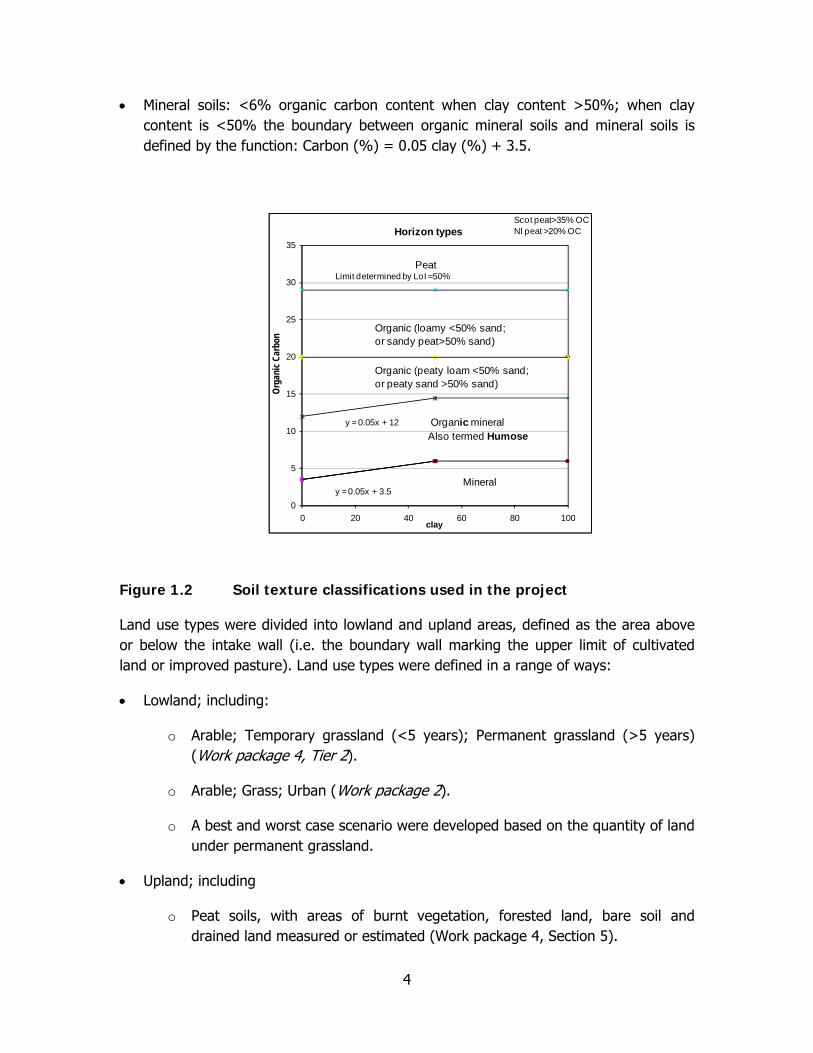
Soils were defined by their texture using a simplified version of the method used by Hodgson (1997), which is illustrated in Figure 1.2. Four soil types are defined and used within this project:

• Peat: >29% organic carbon.

• Organic soils: 14% - 29% organic carbon content when clay content >50%; when clay content is <50% the boundary between organic and organic mineral soils is defined by the function: Carbon (%) = 0.05 clay (%) + 12.

• Organic-mineral soils: 6% - 14% organic carbon content when clay content >50%; when clay content is <50% the boundary between organic mineral soils and mineral soils is defined by the function: Carbon (%) = 0.05 clay (%) + 3.5.

Expert Group MeetingProject plan

Identified work packages

Running of C stocksand fluxes models with inputs/rules

defined by the decision tool forA number of scenarios at the national

scaleReview phase, options appraisal and

Research needs identified

Tier 1 work packages

Tier 2 work package

Individual work packages








Tier 2 work package








Tier 2 work package

Individual work packages

4

• Mineral soils: <6% organic carbon content when clay content >50%; when clay content is <50% the boundary between organic mineral soils and mineral soils is defined by the function: Carbon (%) = 0.05 clay (%) + 3.5.

Figure 1.2 Soil texture classifications used in the project

Land use types were divided into lowland and upland areas, defined as the area above or below the intake wall (i.e. the boundary wall marking the upper limit of cultivated land or improved pasture). Land use types were defined in a range of ways:

• Lowland; including:

o Arable; Temporary grassland (<5 years); Permanent grassland (>5 years) (Work package 4, Tier 2).

o Arable; Grass; Urban (Work package 2).

o A best and worst case scenario were developed based on the quantity of land under permanent grassland.

• Upland; including

o Peat soils, with areas of burnt vegetation, forested land, bare soil and drained land measured or estimated (Work package 4, Section 5).

Horizon types

y = 0.05x + 3.5

y = 0.05x + 12

0

5

10

15

20

25

30

35

0 20 40 60 80 100clay

Organic (peaty loam <50% sand;or peaty sand >50% sand)

Organic mineral Also termed Humose

Mineral

Organic (loamy <50% sand;or sandy peat>50% sand)

Peat

Scot peat>35% OCNI peat >20% OC

Limit determined by LoI =50%Or

gani

c Car

bon

5

o A series of scenarios were developed based on the presence, absence and combination of these characteristics (Work package 4, Section 5).

Further details of these definitions are included in the description of the relevant work packages, as necessary. The methods used in each work package of the project and the results obtained are described in the following section, categorised by the five work packages of Tier 1 and Tier 2.

7

2 WORK PACKAGE 1. RE-EXAMINATION AND INTERPRETATION OF EXISTING SOILS DATABASES AND DATA SOURCES

This work package quantified the uncertainty in baseline soil carbon data and identified the areas of inconsistency between existing UK data sets. The output from this work was a dataset of UK soil carbon data that was derived from the available data and rationalised to be as consistent as possible. The data were fed directly into the decision tool being developed in Work Package 5 in the form of improved estimates of soil C stocks and explicit statements as to their reliability. The decision tool required metadata or summary data, but to ensure these data were consistent and as accurate as possible this work package was aimed at using raw data, mostly under licence, to provide consistency and to highlight mismatches.

The United Kingdom has a number of data sets reporting soil carbon concentrations (as %C) and some reporting soil carbon stocks, reported as either t C ha-1 or kg C m-2 to a given depth. In total, 17 data sets on soil C were identified, of which 14 were eventually obtained for use in the project (the others could not be obtained). Two of the datasets obtained for use in this project are those reporting carbon inventories (collated data) and comprise derived data, so were not used for the estimates of soil carbon content and carbon stocks derived from the original raw measurements. The datasets used and the two collated datasets are shown in Table 2.1.

In many cases access to the data was only possible by purchasing licenses for the use of the data, which slowed down the process of data procurement and had subsequent effects on the timing of the rest of the work. The collation of all these data sets was the first time a serious attempt has been made to combine and create an overarching soil C dataset for UK soils. The resulting “data tool” is a key output of the overall project.

Table 2.1 UK Soil Carbon Data Sets used in this project Data Set Name

Date Owner and or contact

Coverage (E, S, W, NI)

(Relevant) Parameters

Depth(s) C analysis method

No. of samples

National Soil Inventory

1978-1982 Cranfield (Pat Bellamy)

E, W SOC, soil texture land use, bulk density derived using pdf of Howard et al. (1995).

0-15cm <20%C dichromate oxidation; >20%C loss on ignition

5686

National Soil Inventory

2003 Cranfield (Pat Bellamy)

E, W SOC, soil texture, bulk density estimated as above.

0-15cm <20%C dichromate oxidation; >20%C loss on ignition

2361

NSIS 1978-1982 Dr A Lilly S SOC, soil texture, bulk density not measured.

By horizon LOI 3076

8

Data Set Name

Date Owner and or contact

Coverage (E, S, W, NI)

(Relevant) Parameters

Depth(s) C analysis method

No. of samples

NI Soil Data 1995

1995 A Higgins NI SOC, soil texture, land use, bulk density done on selected horizons.

0-7.5 cm and A horizon

LOI 1338

NI Soil Data 2005

2004/5 A Higgins NI SOC, soil texture, land use, bulk density estimates on 0-5 cm horizon only.

0-7.5 cm and A horizon

LOI 583

Woodland survey 1971

1971 Natural England

E, W and S SOC, soil texture, grid reference.

0-15cm LOI 1648

Woodland survey 2001

2001 Natural England

E, W and S SOC, soil texture, grid reference.

0-15cm LOI 1648

Representative Soil Survey Scheme (RSSS)

1969-2002 J Archer E, W SOC, soil texture, land use.

0-15cm dichromate oxidation

>22000

Countryside Survey

1978 NERC CEH

E, S, W, NI SOC, soil texture, bulk density done in 2007 from which pdf derived relating bd to %C. This was used to estimate stocks in 1978 and 1998.

0-15cm LOI (@375oC for 12 hr)

1248

Countryside Survey

1998 NERC CEH

E, S, W, NI SOC, soil texture, bulk density done in 2007 from which pdf derived relating bd to %C. This was used to estimate stocks in 1978 and 1998.

0-15cm LOI (@ 550oC for 2 hr)

1141

ESA Database 1995 ADAS E SOC, texture. 0-7.5cm LOI (converted to SOC using Ball 1964 relationship)

642

ESA Database 1995/1996 ADAS W SOC, texture. 0-7.5cm LOI (converted to SOC using Ball 1964 relationship)

198

Collated Data sets

Soil C inventory data collated by I Bradley for Defra project CC02421

na I. Bradley NSRI

E, W, S and NI

SOC, bulk density dominant soil series, land use.

Not stated Not stated 1240

ECOSSE2 data set

na A Lilly S SOC, soil texture, bd estimated by pdf, 4 land uses.

Horizons LOI 1344

na: not applicable. E = England, S = Scotland, W = Wales, NI = Northern Ireland. LOI = Loss on ignition. bd = bulk density. pdf = pedo-transfer function

9

2.1 Data processing

The data gathered from the various sources were processed into a single data set via four stages:

Stage 1: Removal of records missing either soil carbon content or land use descriptors

Estimating changes in soil carbon stocks resulting from land use changes requires, as a minimum, data on soil carbon content, sampling depth, land use and bulk density. Bulk density is dealt with later; the initial pre-processing removed all those records missing either soil carbon contents or land use descriptors, or both.

Stage 2: Derivation of a simplified soil texture classification based on carbon and clay content

The project reports carbon stocks using a simplified soil classification based on carbon and clay content as shown in Figure 1.2. For mineral and organic mineral soils the clay content is a determinant when it is less than 50%. Where no data on clay content were available, a simplified classifier was used based only on organic carbon with mineral soils defined as <5% organic carbon and organic mineral soils as those with <13% organic carbon.

Where grid references but no soil texture information were available, GIS methodology was used to map the sample location onto the NSRI soil vector map for England and Wales to retrieve the soil series and its soil texture information.

Stage 3: “Normalization” of land use descriptors

Inconsistencies in land use classifications inevitably introduce some error when comparing across data sets. Grassland descriptions are particularly problematic: definitions of permanent and temporary grassland are inconsistent and only two data sets, those from the Countryside Survey, employ the terms neutral, calcareous and acid grassland.

Land use descriptions across the data sets were “normalized” using the protocols set out in Table 2.2.

Stage 4: Derivation of soil bulk density using pedo-transfer functions

Few of the data sets include coincident bulk density measurements. In developing the data tool (see below) it was decided to incorporate two possible pedo-transfer functions to estimate bulk density from other parameters.

The first is:

10

bD = 1.3-(0.275 *ln(Corg/10)) (1)

where bD = soil bulk density (g cm-3)

Corg = soil organic matter content (g kg-1)

This pedo-transfer function is used by Bellamy et al. (2005) but was derived by Howard et al. (1995).

The second is:

bD = 1.29*e-(0.0206)*Corg+2.51*e-(0.0003)*Corg-2.057 (2)

(B. Emmet pers. comm.)

Stage 5: Reformatting data for incorporation in a data tool

Data sets were reformatted for inclusion in a simple Excel-based data tool allowing the user to interrogate the data either within a single data set, or across sets. The field structure is set out below:

Grid reference 10 or 12 character reference (depending on the data set) in the format AA XXXX XXXX or AA XXXXX XXXXX

Land use as set out in Table 2.2

Horizons number of (depth) horizons for which data are available

Date sample date

Lower depth 1 depth in cm of first sample (assumes upper depth=0)

%OC organic carbon content for first depth

Bulk density bD (if available) for first depth

%clay clay content (if available) for first depth

%silt silt content (if available) for first depth

%sand sand content for first depth

Simple texture simplified soil texture (mineral, organic mineral, organic, peat) for first depth

Upper depth 2 top of next sample depth in cm

Lower depth 2 bottom of next sample depth

11

Then the fields “Date” to “Simple texture” repeated for each sample depth.

12

Table 2.2 Land use conversion protocols used in the data tool

Land Use in the Tool

Corresponding Land use in the original data set

NSI Inventory NSI 1984 NSI 2001 CS 1978 CS1998 RSS

EW woodland

1971

EW woodland

2001

England ESA

Wales ESA Ecosse NSIS NI 1995 NI 2005

Arable Arable Arable Arable Arable & hort Arable & hort Arable nd nd nd nd Arable Arable Arable Arable

Woodland woodland woodland forestry

Deciduous Deciduous Deciduous Deciduous broad-leafed woodland

broad-leafed woodland Deciduous

Deciduous woodland/ deciduous

forest/ deciduous

scrub

Deciduous woodland/deciduous

forest/deciduous scrub

Coniferous Coniferous Coniferous Coniferous Coniferous woodland

Coniferous woodland Coniferous

conifer forest/conifer forest/agro-

forestry

Horticultural crops

Horticultural crops

Horticultural crops

Horticultural crops Horticulture Horticulture

Ley grassland Ley grassland

Ley grassland

Ley grassland Ley

grassland Ley grassland

Permanent grass

permanent grass

permanent grass

permanent grass permanent

grass permanent grass

permanent grass permanent

grass

pasture/ pasture

poor/set-aside

Grassland improved grass improved grass grassland

Upland grass upland grass upland grass upland grass

Neutral grass neutral grass neutral grass

Acid grassland acid grassland acid grassland

13

Land Use in the Tool

Corresponding Land use in the original data set

NSI Inventory NSI 1984 NSI 2001 CS 1978 CS1998 RSS

EW woodland

1971

EW woodland

2001

England ESA

Wales ESA Ecosse NSIS NI 1995 NI 2005

Calcareous grassland

calcareous grassland calcareous grassland

Recreation golf

course/urban amenity

Rough grazing rough grazing

rough grazing

semi-natural/rough

grazing Semi-natural/rough

grazing

Saltmarsh salt marsh salt marsh salt marsh

Scrub scrub scrub

Bog bog bog fen/marsh/swamp/bog

fen/marsh/swamp/ bog bog

Upland heath upland heath upland heath upland heath

Lowland heath lowland heath

lowland heath dwarf shrub heath dwarf shrub heath

nd = no data hort = horticulture

15

2.2 The Data Tool

To aid routine interrogations of the data, a simple data tool was developed in Excel. This allows the user to perform the more obvious interrogations routinely (Annex 1). A description of how to use the tool is provided in Annex 1, but due to the strict licensing agreements on UK soils data this tool is not available for use outside this project. 2.3 Using the Data Tool

Only summary results are presented below, to illustrate the possibilities presented by the data sets. Work package 5 and Tier 2 will present the land use change scenario results in detail. Tables 2.3 and 2.4 show the carbon contents and stocks to 15 cm for the main land uses in the 15 data sets. Results with an asterisk are derived from five or fewer records.

Carbon contents of arable soils range from 2.4 – 3.1% for those data sets focused on England and Wales. The Countryside Survey data from 1978 and 1998, although they include Scottish sites, are also in the range 2.7 - 3%. Results from Scotland and Northern Ireland alone are higher, ranging from 3.5 - 5.2%.

The data tool derives both descriptive (i.e. means, standard deviations and skew) and comparative statistics. In general, soil carbon data are not normally distributed and comparative statistics are performed on log-transformed data. The large number of records in some of the data sets means that despite considerable variance, statistical power is high. Thus, the mean carbon content results for arable soils from the NSI 1978 data (1884 records) and those from Countryside Survey in 1978 (251 records) are significantly different (p=0.05) at 3.1 and 3%.

The variation in soil carbon content (0 - 15 cm) across a range of land uses is shown in Figure 2.1 (data derived from the NSI 1978 data set).

16

Figure 2.1 Soil carbon and land use (data derived from the NSI 1978 data set)

Comparisons across data sets for grassland are problematic because many definitions are specific to particular data sets (e.g. only the Countryside Survey used “acid grass”). Acid and upland grass ranges from 3.6 – 18.8% C (0 - 15 cm); rough grazing in England and Wales and Northern Ireland is 10.3 - 12.6%; in Northern Ireland rough grazing ranges from 37.7 - 41.4. The methods of data determination are likely to be less marked than those differences of land use. Why?

The tool also selects data by geographical area based on the National Grid 100 x 100 km grid squares. Figure 2.2 shows the carbon content of arable mineral soils (red points) and grassland organic-mineral soils across a range of grid squares with similar rainfall but differing mean annual temperatures.

Soil carbon and land use

05

1015202530

arab

le

ley

gras

s

perm

anen

tgr

ass

deci

duou

sw

oodl

and

coni

fero

usw

oodl

and

upla

ndgr

ass

%C

(0-1

5 cm

)

17

Figure 2.2 Variation of soil carbon content across a temperature gradient

Initial analysis of these data suggests no discernable temperature signal, but more work remains to be done.

soil carbon vs temperature (medium rainfall)

1.5

3.5

5.5

7.5

9.5

8 9 10 11

Mean temperature (oC 1941-1970)

%C

(0-1

5 cm

)

18

Table 2.3 Carbon content % (0-15cm) for the main land uses across the data sets

*Five or fewer records

Data set NSI Inventory

NSI

1984 NSI

2001 CS

1978 CS

1998 CS

2007 RSS EW

woodland 1971

EW woodland

2001

England ESA

Wales ESA Ecosse NSIS NI

1995 NI2005

Land use

arable 3.0 3.2 2.6 3.0 2.8 - 2.4 - - - - 5.2 3.5 5.2 3.9

woodland 10.7 9.5 10.0 30.0 8.2

deciduous 6.2 5.6 6.8 10.0 16.0* 2.86* 7.6

coniferous 10.0 8.7 20.5 21.9 30.7 39.0 44.8

orchard 3.4 4.01*

hort. crops 4.4

perm. grass 4.6 5.1 4.2 4.5 6.5 6.7

ley grass 5.9 3.8 3.3 2.8 5.7

rough grazing 12.3 10.3 10.6 37.7 41.4

grassland 5.3 5.2 6.6

upland grass 26.7 18.8 31.6

neutral grass 5.3 5.8

calc. grass 9.50* 12.56*

acid grass 24.2 25.8

montane 10.6* 17.1*

bog 40.0 34.0 37.8 51.0

salt marsh 6.2 4.94* 9.84*

scrub 6.4 5.1

upland heath 30.2 18.9 41.4

lowland heath 7.5 8.7 29.8 26.6 39.9

19

Table 2.4 Carbon stocks (kg/km2 to 15 cm) using the CS pedo-transfer function to estimate bulk density

Data set NSI Inventory

NSI 1984

NSI 2001

CS 1978

CS 1998

CS 2007 RSS

EW woodland

1971

EW woodland

2001

England ESA

Wales ESA Ecosse NSIS NI

1995 NI2005

Land use

arable 6.9 7.4 6.3 7.4 6.8 5.8 11.8 8.6 11.7 9.5

woodland 20.0 20.9 21.8 45.1 18.5

deciduous 13.7 13.0 14.2 19.7 27.5* 7.1* 16.4

coniferous 19.0 17.7 33.8 36.0 42.2 56.8 59.3

orchard 8.1 9.7*

hort. crops 9.4

perm. grass 10.3 11.7 10.1 10.8 14.3 15.0

ley grass 12.6 9.2 8.1 7.0 13.0

rough grazing 22.7 21.0

grassland 12.0 12.2 14.8

upland grass 41.6 32.8 48.5

neutral grass 12.3 13.2

calc. grass 21.1* 26.9*

acid grass 39.4 41.8

montane 23.5* 34.5* 58.7

bog 55.5 47.7 50.3 54.3 65.5

salt marsh 13.9 11.9* 22.1*

scrub 13.7 12.1

upland heath 45.8 33.3 57.1

lowland heath 17.1 19.2 45.4 42.5 55.9 *Five or fewer records

20

2.4 Summary

This work package has delivered a methodology to enable the integration and direct comparison of data sets of soil carbon stocks in the UK. These data sets have been quality assured and redefined so that they can be used together; this is the first time this has been undertaken. A data tool has been developed in Microsoft Excel to conduct basic assessments and interrogation of the available data, and the input data for the tool have been derived from multiple raw data sets. The metadata outputs from the data tool feed directly into the decision tool described in Work Package 5 and shown in Annex 2.

21

3 WORK PACKAGE 2. INVESTIGATION OF THE LINKAGE BETWEEN DISSOLVED ORGANIC CARBON FLUX VIA FLUVIAL PATHWAYS AND SOIL CARBON LOSS

This task quantified fluxes of carbon from soils via fluvial transfer as dissolved organic carbon (DOC). Other than soil surveys, DOC data are the only other spatially widespread set of soil carbon data available in the UK, and the only one related to carbon flux. Currently the link between fluvial transport of DOC and soil C is poorly understood. To address this issue, existing data were re-evaluated to assess the impact of refining C flux estimates through a relatively simple assessment of DOC transfer and soil C in a limited number of well-characterised and delineated catchments.

The aims of this task were:

• To understand the land use and soil controls on DOC loss from the terrestrial biosphere, especially the role of mineral soil.

• To use any significant relationships to calculate the flux of DOC from the UK using extrapolation rather than interpolation.

• To estimate the loss of DOC in-stream and quantify the impact of DOC losses from soil on levels of atmospheric CO2 and the loss of DOC at source.

• If relationships were found to be significant, to include DOC flux in the decision tool in Work Package 5.

This work package compared the flux of DOC for a given catchment to the physical characteristics of the catchment. By comparing DOC flux to catchment properties it is possible to compare across catchments, and by allowing for differences in land use and soil type, it becomes possible to compare flux from different size catchments. Any relationships found can then be interpreted and extrapolated. The comparison of DOC flux from different size catchments means that it is possible to measure the amount of DOC lost in streams and to estimate the flux of DOC at source.

This work package drew extensively on the data available from the Harmonised Monitoring Scheme (HMS; Bellamy and Wilkinson 2001). There are 56 HMS sites in Scotland and 214 sites in England and Wales. Data available from the HMS were augmented by data from regular water quality monitoring undertaken by the Environment Agency of England and Wales (EA) and the Scottish Environment Protection Agency (SEPA). This study only considered sites where monitoring was coincident with flow monitoring, otherwise a flux calculation would have been impossible; data were

22

also rejected from any year at any site where there were fewer than 12 samples in that year. Additional data for water colour were converted to DOC concentration by calibrating water colour against DOC concentration for the individual sites using techniques developed by Worrall and Burt (2007).

A wide range of methods have been proposed for calculating river fluxes from concentration and flow data (e.g. De Vries and Klavers 1994). For water quality parameters with a strong seasonal component such as DOC or water colour, Littlewood et al. (1998) recommend the use of “method 5” where data are relatively sparse. However, HMS sampling is generally aperiodic and “method 5” assumes regular sampling. Therefore, an alternative has been proposed here that accounts for differing sampling frequencies:

∑=N

iiy QnCKF1

(i)

y

yy N

An = (ii)

Where: F = the annual flux at the site; Ci = the measured concentration at the site at time i; Qi= the river discharge at time i; K = a conversion factor which takes into account the units used; Ny = the number of samples at the site in that year; and Ay = the number of days in that year, i.e. this can vary with a leap year.

Catchment properties assessed included soil, land-use, and hydrological characteristics. The dominant soil of each 1 km2 grid square in Great Britain was classified into mineral, organic-mineral, and organic soils as previously defined. The land use for each grid square was classified into arable, grass, and urban, based on the June Agricultural Census for 2004. In addition, the numbers of cattle and sheep in each 1 km2 were counted using the census data. The catchment area to each monitoring point for which DOC flux information was available was calculated from the CEH Wallingford digital terrain model which has a 50 m grid interval and a 0.1 m altitude interval. Soil and land use characteristics based on 1 km2 were summed across the catchment areas to the monitoring points for which DOC flux information was available. It was also possible to give a range of hydrological characteristics for each catchment. The hydrological measures used were: the base flow index (BFI; Gustard et al. 1992), the average actual evaporation, and the standard average annual rainfall for each catchment for which DOC flux data were available.

3.1 Statistical treatment of the data

The DOC data were compared to catchment characteristics in a number of ways. First, the DOC data were considered both as the average annual flux for the catchment for the

23

period 2001 to 2007 and as the average annual export (flux/area). Multiple linear regression was used to compare both the average annual flux and the average annual export to catchment characteristics. The regression was used to assess the relationship between average flux, or average export, and the size of the catchment on the basis that if there are significant in-stream losses this should be discernible from the relationship between total flux, or average export. In order to judge the relationship between flux or export, and area, the best-fit significant model was calculated. If the best-fit model included catchment area then the model was recalculated excluding catchment area and the residuals of that model were compared to the catchment area. In using regression to filter the DOC data for effects other than that of catchment area, care was taken to consider information that was a proxy or collinear with catchment area, e.g. area of arable land in a catchment is a collinear with catchment area, but this is less true for percentage arable area within the catchment. For any statistically significant model derived from the multiple linear regression, an analysis of residuals was performed where a standardised residual (residual divided by its standard deviation) greater than 2 was considered an outlier and worthy of further investigation.

Second, the average annual flux, or average export, was compared only with those soil and land use characteristics that are mappable across Great Britain, i.e. any significant relationship found can be applied across Great Britain and then summed across the country in order to estimate the total UK flux. It should be noted that DOC export data were only available for Great Britain and not for Northern Ireland, so it is only possible to map DOC export across Great Britain. However, land use and soil summaries are available for the whole of the UK and so an estimated total DOC flux from the country can be made.

Finally, both average annual flux and export were compared to catchment characteristics using principal component analysis (PCA) in order to assess whether groups or clusters of catchments existed in the data or whether multiple linear relationships exist within the dataset. The PCA was carried out using percentage land use and soil characteristics so that the influence of, and collinearity with, catchment area was minimised. Only the principal components with an eigenvalue >1 and the first with an eigenvalue <1 were considered.

The study updates the papers of Worrall and Burt (2007) and Worrall et al. (2009) who both used HMS data in order to estimate the DOC flux from Great Britain, the former to 2003 and the latter to 2005. Data from the HMS is now available to the end of 2007, so this study first used the same technique as the previous papers in order to update the DOC flux record for the UK and provide a comparison for flux calculations based upon extrapolation from linear models based on catchment characteristics.

24

3.2 Results

Between the years 2000 and 2007 it was possible to calculate a flux for 169 catchments for which complete land use and soil characteristics are available (Figure 3.1). The range of DOC export values in the 169 study catchments varied between 0.1 and 11.8 tonnes C km-2 yr-1 (Table 3.1). A qualitative survey of the data shows that if the extremes are considered then mineral soils have the lowest DOC export, but that the organic-mineral soils appear to have a higher DOC export than the catchments with 100% organic soils (Table 3.1). For comparison of land uses there is no individual catchment that has a single land use as defined by this study. Despite this, by considering the catchments with the maximum of a type it would appear that arable land use has distinctly lower DOC export than either grass or urban land use. However, it will only be possible to understand significant end-members and export coefficients for DOC export after multivariate analysis.

Table 3.1 The annual average DOC export from catchments with the extreme values as defined by dominant soil or land use characteristics used in this project

Catchment characteristic Rivers DOC export (tonnes C km-2 yr-1) 100% Mineral soil Upper Hull, Lee 0.5 – 1.2 100% Organic-Mineral soil Nant-y-Fendrod 6.4 100% Organic soil Mawddach, Ogwen 4.0 – 4.3 71% Arable, 13% Grass Lower Hull 1.3 78% Grass, 4% Arable Taf 4.6 36% Urban, 30% Arable Tame 4.8 Max. Export Wyre 11.8 Min. Export Stour 0.1

25

Figure 3.1 Location of monitoring points for which a DOC export could be

calculated for the period 2001-2007

Using multiple regression the best-fit model for the average DOC flux was developed (Equation i).

Only variables that were found to be significant at least at the 95% level are included in equation (i) and the numbers in the brackets are the standard errors of each coefficient. Note that equation (i) implies that arable land is an active sink of DOC and, furthermore, that there is no loss of DOC with increased catchment area as there is no significant effect due to catchment area. In terms of the annual average DOC export, the best-fit equation is Equation ii.

7.4 4.4 3.5 2.6 2.56.9 3898

(3.7) (0.7) (1.1) (0.3) (0.4)

26

(0.4) (1900) (Eq. i)

r2 = 0.87, n = 169

Where: DOCflux = the average annual DOC flux (tonnes C yr-1); Evapact = actual annual evaporation (mm yr-1); Arable = the area of arable land in the catchment (km2); Urban = the area of urban development in the catchment (km2); Mineral = area of mineral soils in the catchment (km2); OrgMin = the area of organic-mineral soils in the catchment (km2); and Organic = the area of organic soils in the catchment (km2).

:

2 0.03% 0.05% 0.03% 0.024%

(1.0) (0.01) (0.02) (0.01) (0.008) (Eq. ii)

r2 = 0.38, n = 169

Where: %X = the percentage of a given land use (Arable, Urban or Grass) or soil type (Organic), where these terms have the same meaning as for equation (i). Again the percentage of arable land appears to be a sink of DOC and there is no significant role for the catchment area.

Neither equation (i) nor (ii) could be directly extrapolated or mapped across Great Britain. Therefore as an alternative approach, only mappable variables were included in the multiple regression analysis, in which case the best-fit equation was:

3.8 4.8 2.7 2.7 6.7

(1.0) (0.7) (0.3) (0.4) (0.4) (Eq. iii)

r2 = 0.87, n = 169

Equation (iii) could be interpreted as an export coefficient type model. However, as above, the catchment area is not a significant variable. It is possible that other land use descriptors are collinear with catchment area, i.e. the extent of arable land increases with increasing catchment area. Therefore, the negative coefficient for area of arable land (Arable) may not reflect an adsorption of DOC from that land use; rather, it is a proxy for DOC loss with increasing scale. Therefore, as an alternative approach, a model for DOCflux was calculated that definitely included catchment area and then other land use and soil characters were added if they make a significant improvement. On this basis the best-fit equation is:

6.7 2.4 2.6 3.4 9.2 2.7

27

(1.1) (0.6) (0.5) (0.6) (0.6)

(0.5) (Eq. iv)

r2 = 0.86, n = 169

Where: Area = the catchment area (km2).

Although this equation has a marginally worse fit than equations (i) and (iii) it has a suite of coefficients and significant variables that are more physically interpretable and mappable. Equation (iv) can now be physically interpreted, first as an export coefficient model and, second, it demonstrates a significant role for in-stream losses. Equation (iv) no longer predicts that arable land is a significant sink of DOC export and indeed does not predict that it has a significant effect at all. The coefficients of the equation can be directly interpreted as export coefficients (Table 3.2), e.g. the equation predicts that the DOC export from 1 km2 of organic soils would be 9.2 ± 0.6 tonnes C km-2 yr-1 where the quoted error is the standard error in the coefficient. Equation (iv) shows, as would be expected a priori, that mineral soils are a smaller source of DOC than organic-mineral soils which are in turn a smaller source than organic soils (Table 3.2). Furthermore, and as would be expected, the organic soils are a source of DOC more than twice as strong as the organo-mineral soils. Likewise, equation (iv) predicts that both urban and grazed land are sources of DOC, with urban land area being a substantially larger source. The significant role and source size for urban land as indicated by equation (iv) justifies the approach taken by this study in not correcting for waste effluent sources of DOC, as the regression analysis has in effect accounted for it. Of course, grazed land also has a soil type and so grazed land on a mineral soil would be predicted to be releasing DOC at 5.0 tonnes C km-2 yr-1.

As catchment area increases the DOC export would decrease (equation iv), which is direct evidence for in-stream losses of DOC. Equation (iv) suggests that the in-stream loss of DOC is linear with catchment scale. However, the approach taken in the derivation of the equation only allows for a linear response. Therefore, equation (iv) was recalculated using all variables except Area and then the residuals of this new equation were plotted against the catchment area in order to assess the nature of the relationship. This process showed that a linear fit was reasonable and no other relationship was suggested.

Equation (iv) can be used both to map DOCflux on a 1 km2 grid square and to give an estimate of the total DOC flux from the UK (Figure 3.2; Table 3.2). The map shows that, as expected, the areas of high organic soils in the west or north of Great Britain are the important sources of DOC, but urban centres and the lowland peat soils of Eastern England also show up as discrete hot spots of DOC export. Using the export coefficients it is possible to assess the contribution of each significant soil and land use type to the

28

overall flux of DOC from the UK. In this case it can be seen that organic soils represent by far the largest source of DOC, but the loss of DOC in-stream is larger still.

Figure 3.2 The annual average DOC export for each 1 km2 across Great Britain.

Table 3.2 The export coefficient for each significant land use and soil type and the predicted DOC flux from that soil type or land use when considered across the entire UK. The upper and lower estimates are based upon the standard errors in the export coefficients given in equation (iv).

Soil type or land use

Export coefficient (tonnes C km-

2 yr-1

DOC flux (ktonnes C yr-1)

Upper estimate (ktonnes C yr-1)

Lower estimate (ktonnes C yr-1)

Mineral soils 2.6 253.6 302.4 204.9

29

Soil type or land use

Export coefficient (tonnes C km-

2 yr-1

DOC flux (ktonnes C yr-1)

Upper estimate (ktonnes C yr-1)

Lower estimate (ktonnes C yr-1)

Organic-mineral soils

3.4 222.5 261.8 183.2

Organic soils 9.2 588.6 627.0 550.2 Urban 6.7 234.5 273 196 Grazing 2.4 268.6 335.8 201.5 Area -2.7 -658.8 -536.8 -780.8 Total UK flux 909.0 1263.1 554.9 The residual analysis of equation (iv) and application of a critical absolute magnitude to the standardised residual value suggests that there are five catchments that are under-predicted (Rivers Ribble, Weaver, Tyne, North Tyne and Tame) and three catchments that are over-predicted (Rivers Dee, Avon and Severn). It is difficult to discern common features between those catchments that are under-predicted but those that are over-predicted are catchments that are some of the largest in the dataset.

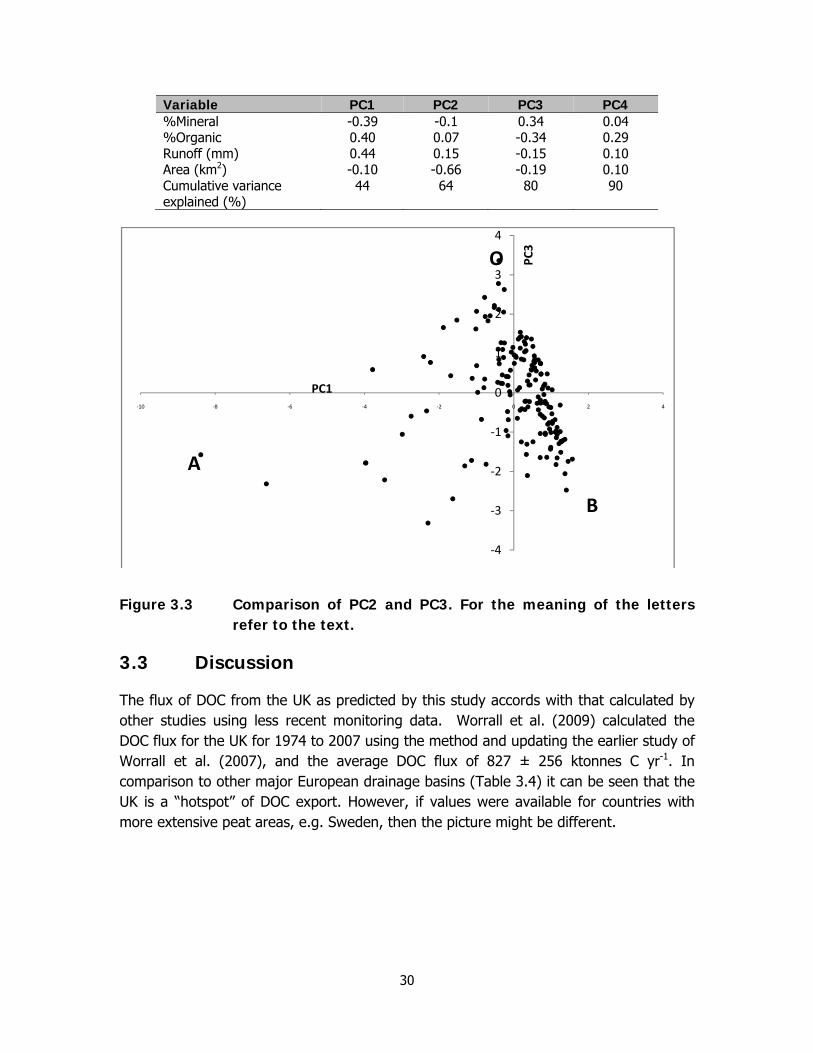
The results including average annual export were inconclusive and only those involving the average annual DOC flux are analysed here (Table 3.3). An examination of the loadings on the principal components shows that it is principal components 2 and 3 that have high magnitude loadings for the average DOC flux while for PC1 and PC4 the magnitude of the loading for the average DOC flux was less than 0.04. For PC2 the pattern of loadings suggests that average DOC flux is correlated with catchment area, i.e. this component represents the increase of DOC with catchment area. The pattern of loadings on PC3 correlates DOC flux with %Urban and %Organic but is negatively correlated with %Grass, Sheepeq km-2 and %Mineral. A plot of PC2 and PC3 showed that all the sites fall within a clear area bounded by two trends (OA and OB – Figure 3.3). The catchments plotting at point O are the Rivers Yeo and Taf, i.e. small catchments with a large proportion of grazing (Table 3.1). Point A is the River Severn, i.e. a large river with a large DOC export, and point B is the River Tame, a catchment with the largest urban proportion (Table 3.1). Therefore, it could be that the PCA is not revealing details of the DOC export but represents contrasts in catchment characteristics in terms of size, land use and soil types. The use of PCA has therefore illustrated that there are no groupings or clusters of catchments with respect to DOC export, and thus a linear model, albeit a multivariate linear regression, is appropriate.

Table 3.3 Loadings on the first four principal components with eigenvalues >1 and the first with an eigenvalue <1.

Variable PC1 PC2 PC3 PC4 Average DOC flux 0.04 -0.65 -0.30 -0.02 %Arable -0.43 0.01 0.18 0.39 %Urban -0.23 0.11 -0.36 -0.78 %Grass 0.29 -0.22 0.55 -0.34 Sheepeq km-2 0.40 -0.21 0.40 -0.13

30

Variable PC1 PC2 PC3 PC4 %Mineral -0.39 -0.1 0.34 0.04 %Organic 0.40 0.07 -0.34 0.29 Runoff (mm) 0.44 0.15 -0.15 0.10 Area (km2) -0.10 -0.66 -0.19 0.10 Cumulative variance explained (%)

44 64 80 90

Figure 3.3 Comparison of PC2 and PC3. For the meaning of the letters refer to the text.

3.3 Discussion

The flux of DOC from the UK as predicted by this study accords with that calculated by other studies using less recent monitoring data. Worrall et al. (2009) calculated the DOC flux for the UK for 1974 to 2007 using the method and updating the earlier study of Worrall et al. (2007), and the average DOC flux of 827 ± 256 ktonnes C yr-1. In comparison to other major European drainage basins (Table 3.4) it can be seen that the UK is a “hotspot” of DOC export. However, if values were available for countries with more extensive peat areas, e.g. Sweden, then the picture might be different.

‐4

‐3

‐2

‐1

0

1

2

3

4

‐10 ‐8 ‐6 ‐4 ‐2 0 2 4

PC3

PC1

O

A

B

31

Table 3.4 Comparison of export values of nitrogen and carbon species for major Western European rivers and the river with the largest DOC export in the world as reported by Alexander et al. (1998) with values derived for the UK from this study.

River basin Size (km2) DOC (kg C km-2 yr-1) Danube 817000 1.21 Elbe 148000 0.81 Po 70000 3.01 Rhine 164500 1.41 Seine 7390 0.91 Nushagak 25000 6.91 UK 244000 2.5 – 8.22 UK (This Project) 244000 2.3 – 5.2

Source of the comparative data, 1Alexander et al. (1998), 2Worrall et al. (2009).

However, this project has gone one step further than these previous studies. All studies cited above give values of the DOC flux at the tidal limit, and not at the source as the DOC leaves the terrestrial biosphere. In the case of this study, it is possible to assess the scale of the source in which the DOC flux at source is 1568 ±232 ktonnes C yr-1, or 6.4 tonnes C km-2 yr-1. Worrall et al. (2007) attempted to estimate the loss of DOC at source for England and Wales only by assuming that the BOD (Biological Oxygen Demand) flux at the tidal limit represents the capacity of the fluvial network to remove DOC; in this case the DOC export at source is equivalent to 5.6 tonnes C km-2 yr-1. However, this latter approach assumes a fluvial residence time in the UK river network of 5 days, i.e. the length of the standard BOD measurement incubation. Furthermore, it is not very surprising that this study gives a larger value of DOC export source than the previous study, as this present study was able to include Scotland, which has a greater proportion of organic soils.

However, it is possible that the DOC flux estimated at source is still an underestimate as the catchments considered here are never smaller than 40 km2, and so this study makes an extrapolation to smaller catchments based on DOC losses for catchments between 40 and 9898 km2. There is field evidence to suggest that in-stream losses of DOC are concentrated in the zero and first-order streams. Worrall et al. (2006) have shown that 40% of DOC is lost across an 818 km2 catchment, but that 32% of that loss is in the first 11.5 km2. In this study the percentage loss varies with the soil and land use type and it has been possible to identify an export coefficient for significant land use types.

The question for this work package in the context of the overall project is, could DOC export ever give an indication of the magnitude or status of the carbon budget of the terrestrial environment? Firstly, there is now doubt that DOC export is a vital component of the terrestrial carbon budget. However, this study suggests that there is still some way to go in using the present routine monitoring of DOC as an indicator of terrestrial carbon budgets. The reason for this is that this study can only go to 40 km2 resolution

32

and we have demonstrated that a large proportion of the DOC may already have been lost from the system before that scale. However, there is another possibility: a number of studies of the net ecosystem exchange of CO2 (NEE) are now well advanced especially for peat soils. In general, for any soil to be a net sink of carbon the following must be true:

. (Eq. v)

Where: NEE = net ecosystem exchange of CO2 (tonnes C km-2 yr-1) = the flux due to DOC, POC, CH4 and diss.CO2 (tonnes C km-2 yr-1).

If it were ever found that the DOC > NEE then that catchment, soil or ecosystem could not be a net sink of carbon regardless of values of POC, CH4 or diss.CO2 flux. Given our improving knowledge of NEE across the UK and for different management and land use settings, it could soon be possible to know what magnitude of DOC export is critical in defining whether an ecosystem is a net sink or net source.

3.4 Summary

The work package has considered records of DOC export from rivers in Great Britain and, by characterising the catchments in which these records were made, has been able to identify the controls on DOC export and provide significant models for explaining this. This work package has:

• Developed models that explained 87% of the variation in DOC flux across 169 catchments;

• Found significant export coefficients for urban and grazed land, as well as for mineral, organo-mineral and organic soils;

• Found a significant decline in DOC flux with increased catchment area, and that this decline is linear across catchment areas from 40 to 9848 km2;

• Mapped DOC export across Great Britain; and

• Estimated that the average annual DOC flux from the UK was 909 ± 354 ktonnes C yr-1, although the loss of DOC at source was 1568 ± 232 ktonnes C yr-1.

It is still probable that the fluxes calculated here are underestimates of the actual DOC flux and, although this study can propose a method for connecting DOC flux to the status of the terrestrial carbon budget, it was not possible to go that far within current datasets.

This work package has identified data gaps in relation to the flux of DOC and has developed a methodology for their measurement, resulting in an estimate of DOC flux

33

for the whole of Great Britain extrapolated from catchment data distributed across the country. However, these data have not at this stage been incorporated into the decision tool as there are too many uncertainties associated with the outputs.

35

4 WORK PACKAGE 3. ACCOUNTING FOR ALL THE CARBON

A number of key areas have been identified that are poorly accounted for in terms of national assessments of soil C stocks and fluxes. These areas do not regularly fall within the remit and modelling estimates of research, where the focus is on either lowland, predominantly mineral soils, or upland peats. The two main areas of potential uncertainty are organic-mineral soils and, particularly, salt marshes, although there are others, such as woodland soils, which also merit consideration.

The importance of these areas for soil C stocks and fluxes has not been clearly understood to date. The aim of this work package was to make a quantitative assessment of the importance of these land use areas and, if appropriate, to include them within the decision tool as a potential additional category to lowlands and uplands. This work package is aimed at ensuring that all the key soil type/land uses in terms of C stocks and fluxes are included in the decision tool in Work Package 5.

4.1 Organic-mineral soils

Organic-mineral soils are extensive throughout the UK (~30% of total soil cover) and make a significant contribution to UK soil carbon stocks and fluxes, in particular through N2O emissions and DOC releases. The soils are typified by shallow upper soil horizons overlying mineral or rock and are particularly prevalent in Scotland and Wales, as shown in Table 4.1. Various regional definitions are used for classifying organic-mineral soils across the UK (e.g. Smith et al. 2007a, Lilly et al. 2009, Holden et al. 2007). All are based on the characteristics of soil profiles and identify organic-mineral soils as those with significant organic matter content in relatively shallow upper soil horizons. In England and Wales organic-mineral soils are those with organic surface horizons <40 cm thick, overlying mineral horizons or rock; the major soil sub-groups associated with such soils in England and Wales are stagnohumic gleys, humic gleys, humic sandy gleys, and humic alluvial gley soils. In Scotland, organic mineral soils have organic surface horizons <50 cm thick overlying mineral horizons or rock, with the organic surface horizon often anaerobic and under waterlogged conditions. Many humus-iron podzols are now cultivated and no longer have an organic surface horizon due to incorporation with the underlying mineral horizons. These soils are mostly humus-iron podzol (uncultivated), peaty podzol, subalpine podzol, alpine podzol, peaty gley, humic gley, peaty ranker (including podzolic ranker), peaty lithosol, and peaty alluvium.

Table 4.1 highlights that organic-mineral soils are fairly extensive throughout the UK, particularly Scotland. The determination of baseline soil carbon stocks and fluxes in these soils would provide an indication of their importance and the need for their inclusion as a separate category in the tool.

36

Table 4.1 Extent of organic-mineral soils in England, Wales and Scotland (% of total land area for each country)

1. Source: Holden et al., 2007. Derived from Landis, England and Wales. 2. Source: Scottish soil survey data, Macaulay Land Use Research Institute.

Several recent reports have assessed the significance of organic-mineral soils with respect to soil carbon stocks and greenhouse gas fluxes (Dawson and Smith 2007, Holden et al. 2007, Lilly et al. 2009a, Lilly et al. 2009b, Ostle et al. 2009, Smith et al. 2007a, Smith et al. 2009, Tomlinson and Milne 2006). The primary aims of this study were as follows:

• Evaluate and revise, if appropriate, the published soil carbon stocks for organic-mineral soils used for inventory assessments (Bradley et al. 2005) using recently published information on soil C stocks of organic-mineral and organic soils.

• Examine the influence of soil parameters on the relative importance of carbon stocks in organic-mineral soils. Several recent studies have reviewed variations in soil carbon stocks. These include soil depth, bulk density, spatial heterogeneity and analytical methods.

4.2 Methods for organic-mineral soils

The study utilised soils information generated in Work Package 1, which provided profile and topsoil data via the soil C and digital soil maps for each country. Data sources included several new or updated nationwide soils datasets, such as the National Soil Inventory for England and Wales (NSIEW); National Soil Inventory for Scotland (NSIS);

Soil type England1 Wales1 Scotland2

Stagnopodzol 1.8 7.3 Stagnohumic gley 3.5 7.3 Humic alluvial gley 1.0 Humic sandy gley 0.1 Humic gley + humic rankers 0.2 1.4 Podzol 1.3 Humus iron podzol 10.8 Peaty podzol 15.5 Subalpine podzol 4.9 Alpine podzol 0.7 Peaty gley 21.8 Humic gley 0.1 Peaty ranker 0.9 Lithosol <0.1. Peat alluvium All organic-mineral soils 6.6 17.3 54.7

37

AFBI Soil Survey for Northern Ireland (AFBI); Representative Soil Sampling Scheme; Resurvey of British Woodlands; and the Countryside Survey of Great Britain. All sampling schemes contain data which can be used to assess the size and significance of soil carbon stocks in organic-mineral soils. Profile data from the NSIEW, NSIS and AFBI have been used previously to generate UK soil C stocks (Bradley et al. 2005).

Characteristic soil profile descriptions for soil series in each country, along with typical values for soil properties, their ranges, and derived functional values were obtained from various surveys and sampling schemes across UK. This was used by Bradley et al. (2005) to calculate soil C stocks across the UK and was subsequently incorporated into the Defra Soil Carbon database. Representative profiles were made available for England/Wales and Scotland from Task 1. These are not entirely consistent with the Defra Soil Carbon database and were not used to generate equivalent UK soil C stocks.

Bulk density (g cm-3), soil carbon value (%) and depth (cm) are the primary components of soil carbon stock calculations, along with spatial extent (km2). To explore the significance of variation in bulk density and soil carbon values, three representative soil series profiles were selected from the National Soil Inventory Profile Database (Table 4.2). The profiles reflect the typical characteristics of a mineral, organic-mineral and organic soil. These profiles were used to explore how variation in soil parameters could alter the contribution of organic-mineral soils to the total UK soil C stock. Spatial extent was assumed to be 73.3%, 19.8% and 6.9% of the UK for mineral, organic-mineral and organic soils respectively (c.f. Bradley et al., 2005).

Table 4.2 Representative series profiles for mineral, organic-mineral and organic soils taken from the National Soil Inventory for England and Wales. Profiles are for permanent grasslands.

Soil type Soil series

Soil sub-

group Horizon* Depth

(cm) LOI (%)

C (%)

Clay (%)

Silt (%)

Mineral CREDITON 5.41

1 20 6.4 3.2 18 43 2 35 2.2 1.1 17 41 3 30 0.8 0.4 14 31 4 65 0.2 0.1 9 22

Organic- mineral WENALLT 7.21

1 20 44.6 22.3 26 36 2 15 4.6 2.3 25 58 3 15 1.8 0.9 17 58 4 20 0.8 0.4 18 53 5 20 0.6 0.3 18 55 6 60 0.4 0.2 13 66

Organic MENDHAM 10.24 1 30 50 25 0 0 2 30 96 48 0 0 3 90 82 41 0 0

*Horizons characterised according to respective soil surveys for England/ Wales and Scotland.

38

Bulk density (dry weight) was estimated by commonly used “pedo-transfer” equations which use available data on other soil properties. Four approaches were used within this study to estimate bulk density:

(A) bD =1.3-(0.275*LN(SOC%)). This equation has been widely used to calculate soil C stocks across Britain (Howard et al. 1995, Bradley et al. 2005, Bellamy et al. 2005).

(B) The approach adopted by Smith et al. (2009) to improve estimates of carbon stocks in organic and organic-mineral soils where;

1) For horizons where soil organic carbon values <28%:

bD = 1.5202 - (0.04716*SOC%)+(0.01251*clay%)-(0.00456*silt%)[eq A]

2) For horizons with soil organic carbon value >20-28%:

bD= 1.77*LN(SOC%) [eq B]

(C) Equation derived from Countryside Survey 2007 (Emmett et al. 2010), adapted to SOC%:

bD = (1.29*EXP(-0.0206*(SOC%*10)))+(2.51*EXP(-0.0003*(SOC%*10))-2.057) [eq C]

(D) An equation derived from the long-term Cockle Park experiment (Shiel and Rimmer 1984):

bD = 1.62-(0.82*LOG10(SOC%)) [eq D]

Where:

bD = bulk density LN = natural log LOG10 = log to the base 10 EXP = exponential

The only source of consistent measurements of bulk density across Great Britain comes from Countryside Survey 2007. These data were obtained from the top 15 cm of the soil profile and are directly comparable to Countryside Survey 2007 values for soil carbon.

Soil carbon stocks (t C ha-1) were calculated for each horizon of the three soil profiles using representative mean percentage data for soil carbon, sand, silt, and clay and all four equations for bulk density estimation. Measured bulk density values from Countryside Survey 2007 were also included for corresponding soil carbon contents. The horizon data were summed to generate the total density of carbon in each

39

representative soil profile (t C ha-1) using each bulk density method. Profile data were then multiplied by area to generate illustrative soil C stocks for mineral, organic-mineral and organic soils in Great Britain using the five bulk density methods. This comparison assessed the influence of bulk density and soil carbon data on data for soil C stocks rather than an actual calculation of soil C stocks for the country. This would require use of the original Defra soil C database to recalculate stocks for all representative soil series using the relative proportions of soil series, along with land cover, in 1 km2. This is an intensive task beyond the scope of the current study.

4.3 The significance of carbon stocks in organic-mineral soils

The primary reference for UK soil C stock estimates is Bradley et al. (2005), who estimated the total UK soil C stock as 1019 Tg based on a unified soil depth of 1 m with the equation for soil bulk density based on Howard et al. (1995). Smith et al. (2007) re-estimated the soil C stocks for organic and organic-mineral soils in Scotland and Wales by incorporating further information on the depth of organic soils and applying an alternative soil bulk density equation. Table 4.3 compares the outcome of these two studies and shows that there is approximately a 1240 Tg difference in mean UK soil C stock estimates, which is primarily accounted for in the revised depth estimates for peats of >1 m depth in Scotland and Wales. Smith et al. (2007) also estimated the stocks for organic-mineral soils to be approximately 20% higher (228 Tg) than Bradley et al. (1995), although there is little variation in the percentage contribution of organic-mineral soils to the UK’s total soil carbon stock (21.5% compared to 22.3%). The main change is a reduction in the relative contribution of mineral soils to the UK’s total soil C stock, with the greater stock values for organic soils (Table 4.4).

Table 4.3 Estimates for UK stocks of soil carbon, with a focus on organic-mineral soils

Data sources Country Total soil C

stock (Mean Tg)

Organic-mineral soils

(Mean Tg)

From Bradley et al. (2005). Stocks estimated to 1 m depth.

England 1740 167 Wales 340 59 Scotland 2187 754 Northern Ireland 296 39 UK 4562 1019

Revised UK estimates: Bradley et al. (2005) for England; revised Scotland & Wales data from Smith et al. (2007); Cruickshank et al. (1998) for Northern Ireland.

England 1740 167 Wales 410 74.5 Scotland 3263 957 Northern Ireland 386 48 UK 5799 1247

40

Table 4.4 Relative contribution of organic-mineral soils to the UK’s total soil carbon stocks

Soil C stock as % of country stocks

Soil C stocks as % of UK stocks

Data sources Country Organic-

mineral Organic Mineral Organic-mineral Organic Mineral

Bradley et al. 2005.

England 9.6 17.0 65.9 3.7 6.5 25.1 Wales 17.4 19.7 53.8 1.3 1.5 4.0

Scotland 34.5 41.3 22.8 16.5 19.8 10.9 NI 13.2 30.4 55.7 0.9 2.0 3.6 UK 22.3 29.7 43.7

Revised UK estimates. 1

England 9.6 17.0 65.9 2.9 5.1 19.8 Wales 18.2 29.6 44.7 1.3 2.1 3.2

Scotland 29.3 54.5 15.3 16.5 30.7 8.6 NI 12.5 42.0 45.2 0.8 2.8 3.0 UK 21.5 40.7 34.4

1. Bradley et al. (2005) for England; revised Scotland & Wales data from Smith et al. (2007); Cruickshank et al. (1998) for Northern Ireland.

4.4 Influence of soil parameters on the carbon stocks of organic mineral soils

4.4.1 Bulk density

Figure 4.1 illustrates the influence of the four different estimates of bulk density as well as measured bulk density on the estimates of soil carbon stocks in representative profiles. This illustrates that the soil carbon stock estimates for the representative profile for an organic-mineral soil are not greatly influenced by the application of different bulk density calculations and that far greater variability occurs when they are applied to organic soils (Figure 4.1). This variability is subsequently transferred to the calculations of UK soil carbon stocks (Figure 4.2).

41

Figure 4.1 Influence of bulk density equations on C stocks of representative soil profiles. Meas=measured CS2007; Ecosse=Smith et al. 2009; Howard=Howard et al. 1995; CS=Emmett et al. 2010; Shiel=Shiel and Rimmer 1984.

measECOSSE

HowardCS

Shiel

mineral

organo-mineral

organic0

200

400

600

800

1000

1200

1400

1600

1800

Tota

l C t

ha fo

r ent

ire s

oil p

rofil

e

bulk density estimation methodsoil type

0

1000

2000

3000

4000

5000

6000

7000

measured ECOSSE Howard CS Shiel

bulk density equations

organicorgano-mineralmineral

simulated

soil C stock (Tg)

42

Figure 4.2 Influence of bulk density equations on the contribution of organic-mineral soils to simulated soil C stocks, using NSI_EW representative soil profiles, CS2007 soils data and area of soils from Bradley et al., 2005. Meas=measured from CS2007; Ecosse=Smith et al. 2007b; Howard=Howard et al. 1995; CS=Emmett et al. 2010; Shiel=Shiel and Rimmer 1984.

Most of the estimates of soil bulk density used in this study assume that bulk density is constant for a given soil organic carbon content. However, Figure 4.3 compares measured bulk density values and soil organic carbon content from the Countryside Survey (2007). This shows that there is a wider variation in bulk density that is not necessarily accounted for in estimated bulk density calculations. One exception is the Ecosse equation (Equation A; Smith et al. 2009), which accounts for variations in silt and clay content when assessing bulk density.

Figure 4.3 Relationship between measured bulk density and soil carbon values from Countryside Survey 2007. Data from NERC.

The variation between measured and estimated bulk densities from Countryside Survey 2007 were also used to investigate the sensitivity of soil C stocks to bulk density. Table 4.5 illustrates ~95% upper and lower confidence intervals associated with estimated bulk density data included within Countryside Survey 2007. These intervals fall within the ranges of values generated by the different bulk density equations at lower SOC contents, but are lower than the estimates from other equations at mid-range SOC

bulk

den

sity

(g c

m3 )

0 10 20 30 40 50 60

soil carbon content (%)

0.0

0.2

0.4

0.6

0.8

1.0

1.2

1.4

1.6

1.8

2.0

43

contents (~28% and ~45%). At this range, there is the greatest variation in estimating bulk density using the four equations (max. 0.44 g cm-3 and min. 0.25 g cm-3). However, the measured data for these soil organic carbon contents are in line with the Countryside Survey data.

Table 4.5 Comparison of measured bulk density (g cm-3) with estimated values and ranges from Countryside Survey 2007 and values from other bulk density equations.

SOC (%)

Measured (g cm-3)

CS eqn Upper range

Lower range

Ecosse Howard Shiel

2.53 1.31 1.20 1.00 1.40 1.45 1.05 1.29 27.50 0.21 0.26 0.18 0.34 0.40 0.39 0.44 45.1 0.18 0.14 0.06 0.22 0.19 0.25 0.26

Figure 4.4 illustrates the effect of this range in estimates of bulk density on calculations of soil carbon stocks by profile, while Figure 4.5 shows their influence when applied to national calculations of soil carbon stocks. This variability has a significant effect on organic and, to a lesser extent, on the organic-mineral soils. These intervals have an obvious influence on the C stock of the representative profile for the organic soils and, to a lesser extent, the organic-mineral soils. These results clearly demonstrate that variation in bulk density will alter the size of the UK soil stock and, to some degree, the contribution of organic-mineral soils to this stock, although this relative contribution is affected primarily by changes in the stocks of organic and mineral soils rather than changes to the stock of organic-mineral soils. The greatest variability in the results would appear to be generated through the relatively poor capacity of all equations to predictive the bulk density of soils with carbon content >~15%. The development of a more robust equation is hindered, in part, by the lack of measured bulk density and associated soils data within the range 15 to 45% SOC. However, the intrinsic variation in bulk density would appear to have a far greater influence than differences between individual estimation methods; at high SOC values this may reflect variations in sampling and analytical efficiencies along with properties such as stoniness and moisture content, rather than clay and silt content.

44

Figure 4.4 Sensitivity of carbon stocks (t ha-1) in representative soil profiles to intrinsic variation in bulk density. CS Eqn = stocks calculated using the CS bulk density equation; Lower and Upper = CS bulk density equation +/- ~95% intervals.

Figure 4.5 Sensitivity of total soil carbon stocks (% Tg) to the intrinsic variation in bulk density. CS Eqn = stocks calculated using the CS bulk density equation; Lower and Upper ranges = CS bulk density equation +/- 95% intervals.

0

500

1000

1500

2000

Lower CS eqn Upper

soil

carb

on (t

ha)

organicorgano-mineralmineral

UEqn

L

organic

organo-mineral

mineral

0

10

20

30

40

50

60

proportion (%)

soil type

45

4.4.2 Soil carbon content

Variation in soil carbon contents between nationwide soil sampling schemes may be due to analytical methods as well as conversion factors. The variation in estimates of percentage soil carbon content has remarkably little influence on the carbon stocks of the representative soil profiles, including that of the organic-mineral soil. This, in turn, has little effect on the total soil carbon stocks or the relative contribution of organic-mineral soils to these stocks. Variations in the estimates of soil carbon content account for ~10% of the variation in total soil carbon stocks from the representative profiles for mineral, organic-mineral, and organic soils. This variation is likely to increase if representative mean values for soil series are used to calculate soil carbon stocks, particularly where higher estimates of soil organic carbon are used.

There are distinct distributions for soil carbon values between the different sampling schemes, reflecting regional differences in the soils being sampled. For example, Countryside Survey and NSIS contain a greater proportion of soils with SOC >40%, reflecting the predominance of organic soils in Scotland. However, the ranges of soil carbon values are similar across all sampling schemes, with the exception of the second sampling of the NSIEW which, unlike the first sample, does not have any soil carbon values above 50%. It is impossible at present to separate out the causes of the discrepancies in soil carbon values between the different sampling schemes or the differences in soil carbon distributions within the NSIEW survey. There has been no widespread use of a common Standard Reference Material (SRM) for the analysis of soil carbon content or loss-on-ignition. This also makes it impossible to produce a comprehensive soil carbon dataset for the UK using all available data sources. This could be remedied by the analysis of a sub-set of samples from all schemes using the same analytical method with an appropriate SRM. A focus would be on resolving the variation in higher soil carbon values, in particular those between 20% and 40% SOC where there are relatively few data points in the UK. Resolution of the causes of variation in soil carbon values across the different sampling schemes would establish a means of directly integrating all available UK soil carbon data and using the information to improve soil carbon stock and change assessments for less well sampled soils, habitats and land uses.

4.5 Summary of findings on organic mineral soils

Organic-mineral soils are responsible for ~21.5% of the UK soil carbon stock based on a revision of country-level stocks using recent data from Scotland and Wales. This is a small and relatively insignificant decline (-0.8%) on IPCC inventory estimates. Increases in the estimates for organic soils are far more significant. If the current carbon stocks for organic soils in England are underestimated due to depth and bulk density, then the relative contribution of organic-mineral soils to UK soil C stocks will be less than 21.5%.

46

Further evaluations of the contribution of organic-mineral soils to UK soil stocks will depend on revisions of stock estimates for organic soils, primarily in England.

Variation in bulk density can be introduced by using different estimation equations or by different methods of field assessment. The variation in estimated bulk density will alter the size of the UK soil carbon stock and the contribution of organic-mineral soils to this stock. This relative contribution is affected primarily by changes in the stocks of organic and mineral soils rather than changes to the stock of organic-mineral soils themselves. A comparison of the estimation equations shows that the greatest differences appear to be a result of the relatively poor capacity of all equations to predict the bulk density of soils with carbon content >15%.

Intrinsic variation in bulk density has a greater influence than differences between individual estimation methods. The Ecosse approach (Smith et al. 2007b) incorporates other soil properties into the equation for soils with SOC <28% to characterise this variation and could be extended to soils with >28% SOC. The development of a more robust equation with relevant confidence intervals is hindered, in part, by the lack of measured bulk density and associated soils data, particularly in the range 20% to 40% SOC.

Actual and simulated variations in soil carbon values, explored using data from the different sampling schemes, had little influence on the carbon stocks of individual representative profiles for organic-mineral, organic, and mineral soils. However, using soil carbon values from the different data sources would produce different UK soil C stock estimates if using the comprehensive Defra Soil Carbon database approach (Bradley et al., 2005). In particular, NSIEW and AFBI would produce lower stock estimates for organic and organic-mineral soils than NSIS, CS and RSBW. These differences would reflect lower estimates of soil carbon at >20%, i.e. ~ 40% soil organic matter content.

Given the range and quantity of soil carbon data that are now available across the UK, consideration should be given to resolving the current discrepancies between and within sampling schemes. The ability to use and interchange all available data would go some way to addressing data gaps in both bulk density and soil carbon values where soil organic matter is greater than 30%, in particular between 32% and 80% SOM. All schemes currently under-sample soils with these levels of SOM, which is reflected in the accuracy of current bulk density estimation methods and the efficiencies of soil organic matter conversions to soil carbon values. UK-wide compatible data would help to improve estimation of stocks and changes in all soil types, including organic-mineral soils.

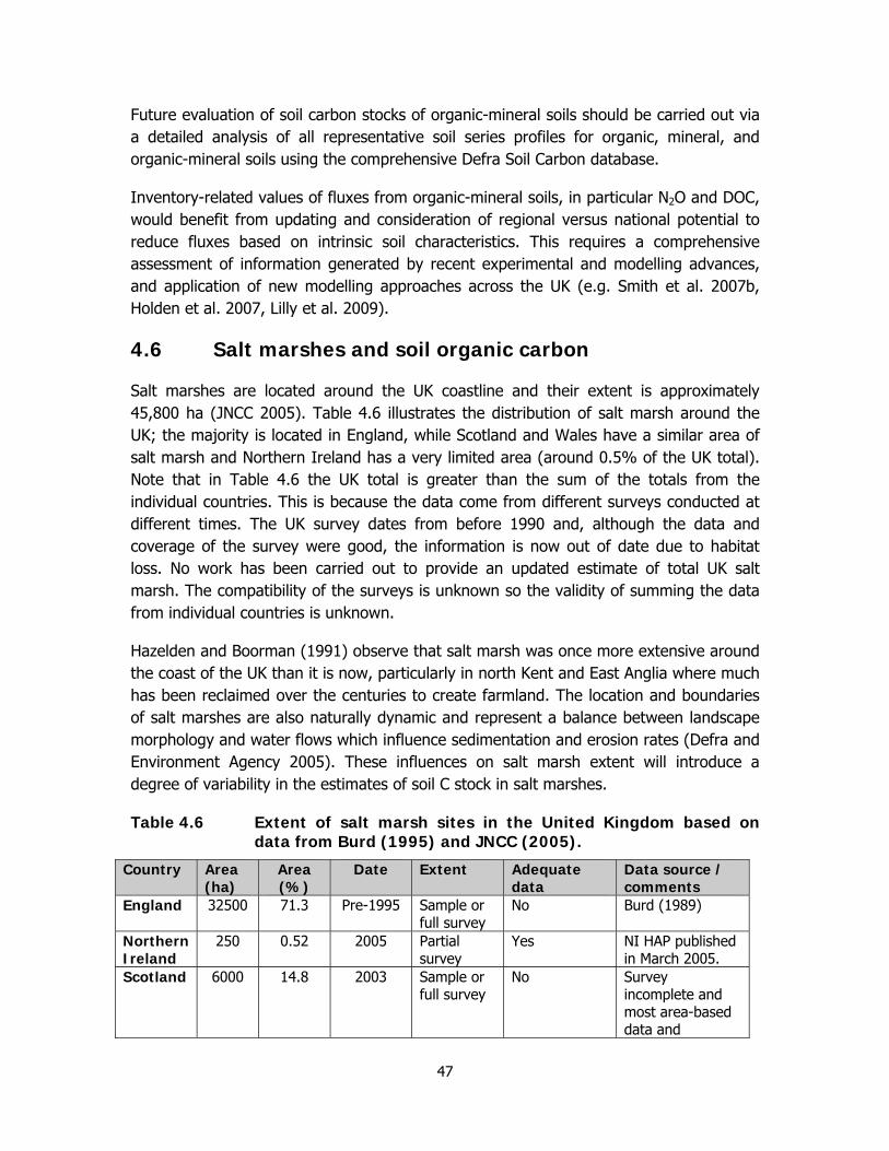
47

Future evaluation of soil carbon stocks of organic-mineral soils should be carried out via a detailed analysis of all representative soil series profiles for organic, mineral, and organic-mineral soils using the comprehensive Defra Soil Carbon database.

Inventory-related values of fluxes from organic-mineral soils, in particular N2O and DOC, would benefit from updating and consideration of regional versus national potential to reduce fluxes based on intrinsic soil characteristics. This requires a comprehensive assessment of information generated by recent experimental and modelling advances, and application of new modelling approaches across the UK (e.g. Smith et al. 2007b, Holden et al. 2007, Lilly et al. 2009).

4.6 Salt marshes and soil organic carbon

Salt marshes are located around the UK coastline and their extent is approximately 45,800 ha (JNCC 2005). Table 4.6 illustrates the distribution of salt marsh around the UK; the majority is located in England, while Scotland and Wales have a similar area of salt marsh and Northern Ireland has a very limited area (around 0.5% of the UK total). Note that in Table 4.6 the UK total is greater than the sum of the totals from the individual countries. This is because the data come from different surveys conducted at different times. The UK survey dates from before 1990 and, although the data and coverage of the survey were good, the information is now out of date due to habitat loss. No work has been carried out to provide an updated estimate of total UK salt marsh. The compatibility of the surveys is unknown so the validity of summing the data from individual countries is unknown.

Hazelden and Boorman (1991) observe that salt marsh was once more extensive around the coast of the UK than it is now, particularly in north Kent and East Anglia where much has been reclaimed over the centuries to create farmland. The location and boundaries of salt marshes are also naturally dynamic and represent a balance between landscape morphology and water flows which influence sedimentation and erosion rates (Defra and Environment Agency 2005). These influences on salt marsh extent will introduce a degree of variability in the estimates of soil C stock in salt marshes.

Table 4.6 Extent of salt marsh sites in the United Kingdom based on data from Burd (1995) and JNCC (2005).

Country Area (ha)

Area (%)

Date Extent Adequate data

Data source / comments

England 32500 71.3 Pre-1995 Sample or full survey

No Burd (1989)

Northern Ireland

250 0.52 2005 Partial survey

Yes NI HAP published in March 2005.

Scotland 6000 14.8 2003 Sample or full survey

No Survey incomplete and most area-based data and

48

Country Area (ha)

Area (%)

Date Extent Adequate data

Data source / comments vegetation data from 1980s.

Wales 5800 13.36 1997 Sample or full survey

No CCW's Lowland Habitat Survey of Wales, 1987-1997

UK 45820 100 Pre-1995 Sample or full survey

No Pre-1990 survey data and coverage good, but now out of date. Habitat loss known especially in SE England.

Table 4.7 summarises current knowledge on trends in salt marshes across the UK. Overall, the area of salt marsh has been declining across the country, with the exception of Northern Ireland. However, it should be noted that in all countries, except Northern Ireland, the available data on both trends and extent are considered inadequate. Field surveys, in combination with aerial or satellite interpretation, are required to update changes to salt marsh extent and status and to improve estimates of current salt marsh soil C stocks.

Table 4.7 Trends in salt marsh sites in the United Kingdom from the JNCC 2005 National Trend Assessment.

Country Trend Date Extent Adequate data

Data source / comments

England Declining (continuing/ accelerating)

2004 Partial survey

No Report to English Nature by Posford Haskoning in 2004 which assessed extent of salt marsh loss in a number of sites, based on interpretation of air photo and other survey data - no new survey was undertaken.

Northern Ireland

Stable 2005 Partial survey

Yes

Scotland No clear trend

2005 Partial survey

No Information recent only for SSSIs. Survey base poorer than other UK countries.

Wales Declining (slowing)

2004 Partial survey

No CCW's Rapid Assessment Survey

UK Declining (continuing/ accelerating)

2005 Best guess No No comprehensive UK-wide assessment of trends. Based on country assessments, it

49

Country Trend Date Extent Adequate data

Data source / comments is likely that the declining trend will continue. Decline is unlikely to be offset by any increases elsewhere in the UK.

4.7 Methods of calculation for salt marshes

The work undertaken within this work package followed the basic principles laid out in Bradley et al. (2005) where soil carbon stocks are estimated from the extent of land use, the soil types within land uses, and the carbon stocks of these soils types. The methods used to achieve this are described in the following paragraphs.

Land use was defined by the Land Cover Map 2000 (LCM2000) sub-level 2 which corresponds to the JNCC Broad Habitat classification and identifies salt marshes as a distinct category. The grid location and area (in m2) for each salt marsh polygon in LCM2000 were identified and calculated and the information used to generate a total area of salt marsh for England and Wales (combined) and Scotland. Available literature was also reviewed to compare the results with previously published data. A spatial overlay of LCM2000 and digital soil maps was used to obtain information on soil types within salt marsh areas for England, Wales and Scotland; appropriate data were not available for Northern Ireland. A significant proportion of salt marsh areas were classified as sea or other non-soil units, due partly (but not completely) to disparities between the two map overlays. Resolution of this issue would improve the accuracy of the information derived from this source and give an improved estimate of soil carbon stocks and fluxes. All soils were converted to the Avery classification of soil groups to estimate the proportion of different soils in salt marshes across Britain (Avery 1980).

Following a similar procedure to Bradley et al. (1995), soil carbon stocks for salt marsh soils to a depth of 1 metre were estimated using representative values and derived functional values for soil series and associations. Estimates for soil C stock in Northern Ireland were obtained by applying representative soil values for Avery soil groups proportionally to the JNCC estimate of salt marsh area in Northern Ireland (250 ha). Soil carbon density (t C ha-1) was calculated for each soil sampling interval in each soil series or association (up to a maximum of seven horizons) using the representative data for organic carbon, sand, silt, and clay (all %) and bulk density. These data were allocated to the dominant land use types in salt marsh areas (i.e. grassland or semi natural land). This information was used to derive total soil carbon densities for representative soil series and associations within the dominant land uses and then used to estimate soil carbon stocks for salt marshes by dominant land use. The term “density” (t C ha-1) is

50

used to distinguish the amount of carbon in a soil profile as opposed to soil carbon stock (Tg), where extent is taken into consideration.

The following equation was applied to estimate soil carbon density (t C ha-1) for individual soil sampling intervals:

Cdensityi = CSOCi * BDi * Depthi * 100

Where:

CStocki = soil organic carbon density per depth interval (i); t C ha-1

CSOCi = soil organic carbon content per depth interval (i); % or g C per 100 g

bD = bulk density of soil fine fractions (<2 mm) at depth interval (i); g cm-3

Depthi = depth of sampling interval; cm

100 = assumes that there are no fractions >2mm. This can be corrected where the proportion of >2mm fraction is known.

Two approaches were adopted to estimate bulk density in this study: these are shown in the section on organic-mineral soils (equations A and B). Soil carbon density (t C ha-1) for entire soil profiles, to a maximum of 1 metre depth, were then calculated for representative soil series and soil associations by the following:

Profile SOCdensityi = Cdensity1 + Cdensity2 + … + Cdensityn

Where:

Profile SOCdensity1-n = total soil carbon density to 1 metre depth for measured profiles of representative soil series or soil associations; t C ha-1.

Cdensity1 + Cdensity2 + … + Cdensityn = sum of soil carbon in each soil sampling interval/horizon to a maximum of 1 metre depth (maximum seven horizons in this instance); t C ha-1.

This method differs from Bradley et al. (2005) as it only calculates the total soil carbon density using available data for sampling depths. There has been no estimation of Cdensity below actual sampling depths, e.g. where the soil profile was less than 1 metre deep. Bradley et al. (2005) also calculated Cdensity at 0 to 30 cm and then 30 to 100 cm. For England and Wales, soil profile carbon density by soil series information was used to calculate mean soil carbon density (+ 1 standard deviation) by major soil subgroup. Soil carbon stocks (Tg) for salt marshes were then calculated by the following:

51

SOCstocka-n= (Profile SOCdensitya * Areaa) + (Profile SOCdensityb* Areab) + … + (Profile SOCdensityn* Arean) * 10-6

Where:

SOCstocka-n = total soil carbon stock of salt marshes to 1 metre depth for the two dominant land uses in each region (Tg);

Profile SOCdensitya = representative soil carbon density of major soil subgroup or soil association (t C ha-1);

Areaa = Area of major soil subgroup or soil association within salt marshes (km2);

For areas of unknown soil type, ProfileSOCdensity was estimated as an average of the representative soil types recorded in salt marshes.

4.7.1 Area of Salt Marsh

The total area of salt marsh in Great Britain (England, Wales and Scotland) was estimated at 45,771 ha. This compares favourably with previously published information, as illustrated in Table 4.3; the discrepancies are likely to be a reflection of the methods of estimation used and uncertainties over data. For example, the JNCC estimates were primarily derived from pre-1995 field surveys and are considered incomplete. Cannell et al. (1995) estimated a far lower salt marsh extent in Scotland and a greater extent in England, which may reflect the attribution of salt marshes at national boundaries. The low area of salt marsh reported for Northern Ireland (76 ha) has been superseded by more recent and relatively good data which identified 250 ha of salt marsh in this region (Table 4.8).

Table 4.8 Extent of saltmarsh sites (ha) in the United Kingdom obtained from this study compared with previous estimates.

*see earlier text

Soils of salt marshes: The results from overlaying national soil maps with LCM2000 are presented in Table 4.9. These highlight that salt marsh soils are dominated by alluvial gley soil types (~62%). However, a significant proportion (~48%) may consist of a wide

Regions This study (derived from

LCM2000)

JNCC 2005 Boorman 2003

Cannell et al. 1995

England 33,261 32,462 32,500 35,200 Wales 5,981 5,800 6,039 6,160 Scotland 6,469 6,000 6,748 2,640 GB 45,711 44,262 45,287 44,000 Northern Ireland * 250 239 76 UK 44,512 45,526 44,076

52

diversity of other soils (>30 soil groups). These may reflect conversion of salt marshes to agricultural use along with natural soil development in salt marsh/coastal areas. None of these soils contribute >7% of the total area of soils in salt marshes. It is difficult to establish just how diverse soil types are within salt marshes. There have been few field surveys in this habitat type, while there is a lack of habitat information associated with historical national scale soil surveys. However, this diversity has some significance for calculating soil C stocks (see below) and for estimating GHG emissions.

Table 4.9 Soils associated with salt marshes in England, Wales and Scotland. Classification according to Avery (1980).

4.7.2 Regional soil carbon stocks in salt marshes

The results for regional soil carbon stocks for two land use types (permanent grassland or other semi-natural land use) and using two soil bulk density equations are presented in Table 4.10. The range of total C stock for salt marshes in England and Wales is 9.841 to 13.696 Tg C, and 1.115 to 2.301 Tg in Scotland. Although there is a significant range in these soil C stock estimates, the overall contribution of salt marshes to regional C inventories is relatively small.

The results imply that land use has a significant influence on the carbon stocks in salt marshes, with greater stocks in soils with the least intensive agricultural management. However, the results also demonstrate that the estimates of bulk density introduce significant variation in stock values. Using equation A, the average bulk density was 0.726 g cm-3 and using equation B it was 1.266 g cm-3. Equation A is closer to the bulk density estimates used by Cannell et al. (1995). However equation B considers the presence of clay and silt in soils with SOC <20%, while equation A does not. In addition,

Soil groups from Avery

% salt marsh area

Description

2.2 43.24 unripened alluvial gley soils

8.1 19.02 alluvial gley soils

5.4 6.77 brown earth soils, loamy and non-alluvial Unclassified 5.59

7.1 4.45 stagnogley soils, seasonally waterlogged

3.6 4.41 sand pararendzina; unconsolidated calcareous sandy deposits other than alluvium

5.7 2.28 argillic brown earths, loamy soils with signs of clay enrichment

8.5 1.90 humic-alluvial gley soils, with enriched organic matter topsoil

8.4 1.87 argillic gley soils, waterlogged with clay enrichment 6.1 1.27 brown podzolic soils

Remaining groups with small coverage 9.20

ca. 24 soil groups

53

this study only estimated soil C stock to 1 m depth, following the procedures of Bradley et al. (2005). This limitation is likely to underestimate the total C stock in salt marsh soils significantly since the profiles of these soils can reach several metres in depth (Chmura et al. 2003).

Table 4.10 Soil carbon stocks (Tg) in saltmarshes by land use and region. C stock A = using Howard et al. (1995) bulk density equation and C stock B = using modified Smith et al. (2007) bulk density equation.

4.8 Influence of soil type on soil carbon stocks

There is a degree of uncertainty over the proportions of different soil types in salt marshes due to a lack of field survey information. To investigate the potential influence of this heterogeneity, soil C stocks were recalculated assuming that all soils would be alluvial soil types (Equation B). The results (Table 4.11) indicate that soil C stocks would be significantly higher in most instances, reflecting differences in both bulk density and carbon content in the upper soil horizons. Estimates of salt marsh soil C stocks would benefit from more accurate mapping of soil types within this habitat.

Table 4.11 Influence of soil type on soil carbon stocks (Tg) in salt marshes. Estimated C stock assuming all soils are alluvial gleys and difference (%) to C stocks assuming a diversity of soil types (from Table 4.10).

Regions Land use

Soil C A stock to 1 m depth (Tg); Eqn

A

Soil C B stock to 1 m depth (Tg); Eqn B

England and Wales Permanent grassland 9.841 12.706 Other semi-natural 10.005 13.696

Scotland Grassland 1.115 1.624 Other semi-natural 1.974 2.301

Regions Land use

Soil type and % difference against range of soil types

C stock A (Tg)

C stock B (Tg)

England and Wales

Permanent grassland

Alluvial 14.077 18.083 % difference 143 142

Other


Scotland

Grassland


Semi-natural Alluvial 2.318 2.815 % difference 208 173

54

4.8.1 Estimates for soil carbon stocks in UK salt marshes

Table 4.12 shows estimated soil carbon stocks in UK salt marshes by country, which is between 10.982 to 26.823 Tg. This represents 0.24 to 0.59% of the UK’s total soil C stock (4562 Tg), as estimated by Bradley et al. (2005). In England and Wales salt marshes account for <1.15% of soil C stock and 0.26% of regional land cover. In Scotland the equivalent figures are <0.12% from 0.08% of land cover. These differences imply that the soils in salt marshes of England and Wales are relatively high in carbon content compared to other land uses, but this is not the case in Scotland where soils of relatively high organic matter predominate in all land uses.

Table 4.12 Estimated carbon stocks of salt marsh A = using Howard et al. (1995) bulk density equation and B = using modified Smith et al. (2007) bulk density equation. Northern Ireland values are estimated from available data sources.

4.8.2 Sequestration of carbon in salt marsh soils

Cannell et al. (1995) estimated that the sequestration of carbon on salt marshes (i.e. accretion from sedimentary and fluvial processes) was <0.1 Mt C yr−1 + 20%. Based on average topsoil C contents of salt marsh soils in England, Wales and Scotland, this would equate to an annual increase of 0.3 mm in topsoil depth. Brew and Pye (2002) suggest that vertical accumulation of sediment in certain salt marsh areas could reach 70–100 cm over the next century. Therefore, taking a maximum potential accumulation rate of 1 cm per year, the rate of C sequestration in salt marsh soils would be 0.25 Mt C yr−1 in England and Wales, and 0.08 Mt C yr−1 in Scotland, and total C sequestration across the UK would be 0.33 Mt C yr−1. It should be borne in mind that estimates from this study are based on generic and historical statistics for accretion rates in UK salt marshes. They

Soil type Regions C stock A (Tg) C stock B (Tg)

Grassland (permanent)

Other/Semi-natural

Grassland (permanent)

Other/Semi-natural

100% alluvial

England and Wales

14.077 17.912 18.083 23.899

Scotland 1.374 2.318 1.585 2.815 Northern Ireland

0.066 0.09 0.076 0.109

UK 15.517 20.32 19.744 26.823

Range of soil types

England and Wales

9.841 10.005 12.706 13.696

Scotland 1.115 1.974 1.624 2.301 Northern Ireland 0.026

0.030 0.035 0.043

UK 10.982 12.009 14.365 16.040

55

do not account for any substantial losses in salt marsh area, which could significantly reduce this sequestration rate. Contemporary and preferably site-level data would be required for validation, taking into account potential C losses through DOC (e.g. Boorman et al. 1994, Tappin et al. 2003).

Although CH4 fluxes are negligible, salt marshes can be sources of N2O, especially in estuaries where there is nutrient enrichment. Although there have been no extensive field assessments of GHG emissions across the range of UK salt marshes, site surveys and modelling exercises indicate that the global warming potential of salt marsh soils through N2O emissions is relatively low and contributes <1% to UK inventory calculations (Sozanska et al. 2002, Kenny et al. 2004).

4.9 Summary of findings on salt marshes

This is the first assessment of soil profile carbon stocks in UK salt marsh soils and it has established that salt marshes contribute <0.59% to the UK’s total soil carbon stock. However, these soils could be sequestering C at relatively fast rates compared to other soil types, and at higher rates than previously estimated. With respect to GWP, salt marsh soils appear to remain relatively small sources of N2O, which could be further reduced through reductions in nutrient enrichment. There remain various sources of uncertainty in estimating soil carbon stocks and fluxes in UK salt marshes, which could be reduced through:

• Improved estimates for the extent of UK salt marshes and the heterogeneity of soil types within salt marshes;

• Improved information on the land use and management of UK salt marshes and how these relate to soil types;

• Improved data on the characteristics of salt marsh soils to include depth of UK salt marsh soils, carbon content to depth, and measured bulk densities; and

• Integrated field assessments that could assess the global warming potential of UK salt marshes by accounting for both C accumulation, through processes such as accretion and root inputs, and GHG fluxes.

4.10 Summary

This work package has improved understanding of the influence of organic-mineral soils on soil carbon stocks in a typical soil profile and extrapolated this information to provide an estimate of UK soil carbon stocks for organic-mineral soils in relation to organic and mineral soils.

56

This work package has also quantified the extent of salt marshes around the UK and established the potential carbon stocks and fluxes associated with this land area that were previously unaccounted for. Although there is scope for refinement of the estimates provided, the indication is that salt marshes account for a relatively low percentage of the UK soil carbon stock and flux.

57

5 WORK PACKAGE 4. THE DEVELOPMENT OF LAND USE AND MANAGEMENT SCENARIOS

The spatial extent of land use change in ”change in C per hectare” must be defined in order to interpret the outputs of the decision tool (Work Package 5). A range of scenarios was delineated, representing the reasonable extremes of land management in the UK, and these are presented below. This work package provided areas of land use change at a national level with reference to soil C stocks and fluxes. These situations were used directly in Tier 2 to extrapolate the outputs of the decision tool to a county and national scale.

5.1 Lowland scenarios

Three scenarios were considered for managed agricultural land in lowland Britain:

1. Business as usual – recent day (2004 baseline year) land use & management.

2. Historical “best case” – interwar period (i.e. 1930): maximum area of grassland (and associated soil C storage).

3. Potential improvement scenario – arable reversion to permanent grassland in groundwater protection zones.

Agricultural census statistics (dating back to 1890) were used to determine the area of the following land uses at a county level (using current county boundaries) in lowland Britain for each scenario (Anon 1968; Comber et al. 2008):

• Permanent grassland (>5 years)

• Temporary grassland (<5 years)

• Tillage land

The current area of woodland was also determined for the ”business as usual” scenario, using the Forestry Commission’s National Inventory of Woodland and Trees. Each area was broadly divided according to soil type (mineral <5% SOC; organic-mineral 5 - 12% SOC; organic >12% SOC) using National Soils Inventory data for England and Wales (McGrath and Loveland 1992) and Scotland (Lilly et al. 2009b).

The “potential improvement scenario” was developed using 2004 as a baseline, with all tillage land within groundwater protection zones reverted to permanent grassland. In this case, the 1998 Nitrate Vulnerable Zones were considered (SI 1998), which were largely within England (334 ha) with a small area of Wales (0.33 ha).

58

Outputs were in the form of an area in millions of ha for each land use and each scenario, to be fed directly into the Tier 2 modelling exercise. In addition, estimates of the total topsoil (0 - 15 cm) C stocks for managed agricultural land (tillage, temporary and permanent grassland) within each of the scenarios were calculated using average soil C contents for each land use obtained from the NSI and NSIS databases, assuming a standard bulk density of 1.3 g cm-3 (Table 5.1).

Table 5.1 Topsoil (0-15 cm) carbon stocks for tillage, temporary and permanent grassland in Britain.

Land use England and Walesa Scotlandb % C t C/hac % C t C/hac Arable (tillage) 3.13 61.0 3.54 69.0 Temporary grassland 3.84 74.9 4.95 96.5 Permanent grassland 5.05 98.5 7.24 141.2

aNSI 1983 (Cranfield University) bNSIS 1985 (Macaulay Institute) cAssumes ”standard” bulk density of 1.3 g cm-3 and soil depth of 15 cm (i.e. 1950 t ha-1 topsoil)

Estimates of the amount of C stored under arable-reversion grassland (”potential improvement scenario”) were determined using the C stock under tillage (arable land) and applying a C accumulation factor of 0.44 t C ha-1 yr-1 (Smith et al. 2007c) for a period of 20 years.

5.2 Upland scenarios

Due to the paucity of data for some upland scenarios, it was necessary to use the Durham Carbon Model in order to assess the equivalent CO2 budget of upland peat soils and to calculate the equivalent CO2 budget of selected regions of peat soils under a range of management and land use scenarios (Worrall et al., 2009). The modelling considered five regions of upland peat soils (Table 5.2). The regions were selected to give an adequate sample of UK upland peat soils from which national estimates could be extrapolated. For each region an area of at least 100 km2 was selected where, for each 1 km2 grid square (grid squares set to coincide with the Ordnance Survey National Grid), peat soil covered at least 10% of that 1 km2. The classification of soils for each 1 km2 grid square was on the basis of the HOST classification (Boorman et al. 1995). Once an area of at least 100 km2 had been defined then a recent, geo-referenced aerial photograph of each 1 km2 within that area was examined and the land management on the peat soils classified as to the percentage of each grid square that showed evidence of burn management, drainage, bare soil, and forestation. The presence of burning as identified from aerial photographs does not give an indication of the frequency of burning in that area. Therefore, it was assumed that burn frequencies could reasonably be between 10 and 20 years and the exact frequency of burning was randomly estimated as an integer value from a uniform distribution between these two values.

59

Furthermore, the year of burning was randomly assigned within the model run period. Wherever drains were identified in the aerial photographs the drain spacing was measured; otherwise it was randomly assigned a drain spacing of between 10 and 20 m, based on previous experience in these regions (Worral et al. 2006). For each region the Durham Carbon Model was run for the following scenarios:

• Business as usual – the land use is set as described above with no intervention.

• Cessation of managed burning – as if there was no managed burning at any time during the period from which data were reviewed or before.

• Cessation of grazing – there is no grazing during the study period.

• Blocking of all drains and gullies – the presence of all drains and gullies is removed as if they had never existed at the start of the study period.

• Re-vegetation – the percentage of bare soil is decreased to a small default value of 1%.

• All possible interventions.

Each scenario was run for the 10 year period 1997 - 2006 and the average CO2 budget for the 10-year period used as the budget estimates. A 10-year study period was taken so that the result averages across flood and drought years. In total, 10308 model runs were considered covering 1718 km2.

Table 5.2 Land management characteristics of the regions selected for this study.

Region Area surveyed

(km2)

Drained/gullied (km2)

Bare soil

(km2)

Grazed (km2)

Burnt (km2)

Afforested (km2)

Peak District 550 134 20 527 186 23 Nidderdale (Yorkshire Dales)

471 52 13 460 111 11

Galloway (South West Scotland)

352 0 4 154 0 198

Migneint (North West Wales)

235 28 6 214 6 21

Dartmoor 110 3 1 109 0 1 Total 1718 217 (12.6%) 44

(2.5%) 1464

(85.2%) 303

(17.6%) 254

(14.8%) In order to make the assessment the data were sorted by the management types that can be considered by the Durham Carbon Model (presence/absence of: burning, grazing, drainage, bare soil, or forest plantation), and the predicted budgets were then assessed using analysis of variance (ANOVA) in order to assess which management or land use interventions had a significant effect upon the equivalent CO2 budget. On the basis of

60

the significant differences found, land use factors could be derived and confidence limits calculated on these.

The emission factor for CH4 is expressed separately from all other carbon uptake and release pathways and is expressed as tonnes CH4/ha/yr. All other carbon release pathways are expressed in terms of their CO2 equivalence (expressed as tonnes CO2/ha/yr) and, in order to do this, atmospherically-active equivalence of the fluvial loss components has to be judged. In order to account for the atmospherically-active component of fluvial flux this study makes the following assumption:

PPCOdissDOCrespequi COCOCOCOCO 2.2222 24.0 −++= (Eq. vi)

Where: CO2equi = total equivalent CO2 budget of the area (tonnes equivalent CO2 ha-2 yr-

1); CO2x = annual equivalent CO2 budget (tonnes equivalent CO2 km-2 yr-1) where x is: resp = net ecosystem respiration; DOC = fluvial flux of DOC; diss.CO2 = annual dissolved CO2 flux; and PP = annual uptake from primary productivity.

This approach to understanding fluvial flux is based upon a conservative approach from field observations (Worrall et al. 2006). It should be noted that this approach assumes that carbon lost as POC is not atmospherically-active and is not based on the value of DOC loss in-stream calculated elsewhere in this project.

By convention, the vector of each emission factor expressed as a positive is in fact a loss from the soil and a gain to the atmosphere.

The land use and management observations from Table 5.2 are combined with emission factors for CO2 and CH4 over the following scenarios:

1. Business as usual – the present distribution of land use is used as outlined in Table 5.3.

2. Realistic worst-case – the realistic worst case can be viewed in several ways as it is not possible for peat soils to be both afforested and to be managed as grouse moor at the same time. Therefore, the worst case scenario is a choice of the combination of how much land to ascribe to afforestation and grouse moor management. This study considers that afforestation doubles and that the remaining land is then grazed, drained and comes under burn management.

3. Best case – in this case all peat soil areas are restored to pristine condition, i.e. all drains are blocked, all burning ceases, grazing is removed, bare soil is revegetated, and forestry is restored to blanket bog.

61

5.3 Results for lowlands

Table 5.3 gives the areas associated with each land use and scenario for use in the Tier 2 modelling exercise.

Table 5.3 Total area of managed agricultural land and woodland (million hectares) for each scenario in England, Wales and Scotland.

Scenario & country

Tillage Temporary grassland

Permanent grassland

Total managed

Woodlanda

Business as usual (2004) England 4.41 0.66 3.05 8.12 9.18 Wales 0.07 0.10 0.98 1.15 1.42 Scotland 0.74 0.27 0.75 1.76 3.1 GB total 5.22 1.03 4.78 11.0 13.7 Historical “best” (1930) England 2.56 0.80 5.30 8.66 nd Wales 0.15 0.12 0.87 1.14 nd Scotland 0.64 0.61 0.63 1.88 nd GB total 3.35 1.53 6.80 11.7 nd Potential improvement England 4.08 0.66 3.38b 8.12 nd Wales 0.07 0.10 0.98b 1.15 nd Scotland 0.74 0.27 0.75 1.76 nd GB total 4.89 1.03 5.11 11.0 nd

aTaken from NIWT database (Forestry Commission) for the current “business as usual” scenario only (2004). b0.33 ha of arable reversion grassland in England, 340ha in Wales. nd = no data.

For each scenario the total area of managed agricultural land was very similar at approximately 11 million hectares, with a slightly greater area (0.7 m ha) of managed agricultural land in 1930. There was also a considerably greater area of permanent grassland (2 million ha) in 1930 compared to the present day. All of this additional grassland was in England, with a proportionally lower area of tillage land. Conversion of tillage land to permanent grassland within the 1998 NVZ regions of England (SI 1998) only resulted in a very small increase in the total grassland area, compared with a 2004 baseline.

Table 5.4 shows the changes in C stocks in managed agricultural land for each scenario. Total topsoil (0 - 15cm) C stocks for managed agricultural land ranged from 910 mT in 2004 to 1032 mT in 1930, and were of a similar magnitude to those reported by Bradley et al. (2005) for arable and pasture topsoils (0 - 30 cm) in Britain. There was an estimated 120 mT (12%) reduction in topsoil C stocks in managed agricultural land between 1930 and 2004, largely due to the 30% reduction in permanent grassland area (Table 5.4), although there was also a small (c. 6%) decrease in the total managed agricultural land area during this period.

62

Table 5.4 Total topsoil (0-15 cm) C stocks (million tonnes) in managed agricultural land for each scenario in England, Wales and Scotland.

Scenario & country Tillage Temporary grassland

Permanent grassland

Total managed

Business as usual (2004) England 269 50 300 619 Wales 4 8 96 108 Scotland 51 26 106 183 GB total 324 84 502 910 Historical “best” (1930) England 156 60 522 738 Wales 9 9 85 103 Scotland 44 59 88 191 GB total 209 128 695 1032 Potential improvement England 249 50 323a 622 Wales 4 8 96 108 Scotland 51 26 106 183 GB total 304 84 525 913

a300mT in permanent grassland and 23 mT in arable reversion grassland, assuming a C accumulation rate of 0.44 t ha-1 yr-1 over 20 years (Smith et al. 2007b).

Arable reversion to grassland in ground water protection zones only had a very small impact on estimated C stocks (0.3% increase or 3 mT). Smith et al. (2007c) suggested C accumulation following land use change from arable to grassland would be in the range -0.02 to 0.9 t ha-1 yr-1, with a mean of 0.44 t ha-1 yr-1 (used in this scenario). Even using the higher estimate of C accumulation, the total impact on C stocks is small (5 mT or 0.6% increase).

5.4 Results for uplands

Given the estimates of the area of UK peat the results for the scenarios outlined are given in Table 5.5 and suggest that UK peat soils are a considerable sink of GHG and would remain so even with major land use intervention. However, these estimates have several important limitations:

1. Validation - the analysis is based on results from the Durham Carbon Model and not from field observations. The Durham Carbon Model has been calibrated against field observations, but it has never been validated for any site.

2. Altitude - the model predicts that altitude is a significant covariate controlling the GHG flux from a peat soil. The distribution of peat soils with altitude was not available to this study but it should be noted that the model predicts that the largest sinks of GHG will be at sea level.

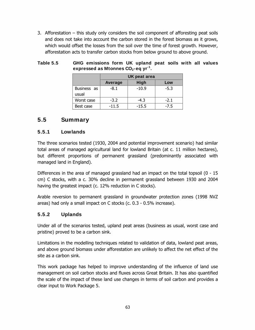
63

3. Afforestation – this study only considers the soil component of afforesting peat soils and does not take into account the carbon stored in the forest biomass as it grows, which would offset the losses from the soil over the time of forest growth. However, afforestation acts to transfer carbon stocks from below ground to above ground.

Table 5.5 GHG emissions form UK upland peat soils with all values expressed as Mtonnes CO2-eq yr-1.

UK peat area Average High Low

Business as usual

-8.1 -10.9 -5.3

Worst case -3.2 -4.3 -2.1 Best case -11.5 -15.5 -7.5

5.5 Summary

5.5.1 Lowlands

The three scenarios tested (1930, 2004 and potential improvement scenario) had similar total areas of managed agricultural land for lowland Britain (at c. 11 million hectares), but different proportions of permanent grassland (predominantly associated with managed land in England).

Differences in the area of managed grassland had an impact on the total topsoil (0 - 15 cm) C stocks, with a c. 30% decline in permanent grassland between 1930 and 2004 having the greatest impact (c. 12% reduction in C stocks).

Arable reversion to permanent grassland in groundwater protection zones (1998 NVZ areas) had only a small impact on C stocks (c. 0.3 - 0.5% increase).

5.5.2 Uplands

Under all of the scenarios tested, upland peat areas (business as usual, worst case and pristine) proved to be a carbon sink.

Limitations in the modelling techniques related to validation of data, lowland peat areas, and above ground biomass under afforestation are unlikely to affect the net effect of the site as a carbon sink.

This work package has helped to improve understanding of the influence of land use management on soil carbon stocks and fluxes across Great Britain. It has also quantified the scale of the impact of these land use changes in terms of soil carbon and provides a clear input to Work Package 5.

64

6 WORK PACKAGE 5. THE DEVELOPMENT OF SOIL CARBON STOCKS AND FLUXES DECISION TOOL

The objective of this work package was to develop a decision tool capable of providing a quantitative estimate of the ”per hectare” soil C stock change and flux for several land use change scenarios. Land use change and land management change have significant greenhouse gas mitigation potential globally. Smith et al. (2007c, 2008) estimated the yearly global mitigation potential in agriculture to be 4200, 2600 and 1600 Mt CO2-eq. yr-1 at 100, 50 and 20 United States Dollars (USD) per tonne CO2-eq-1, respectively. The mitigation potential is cost-competitive with other potential management options in other sectors (Barker et al. 2007), showing that land use has a significant role to play in addressing climate change. Change in land use may lead to changes in soil carbon content (Guo and Gifford 2002; Smith et al. 2000a), with different tillage practises reducing the SOC stock (Guo and Gifford 2002; Johnston 1973). Similarly, when croplands are converted to grasslands or woodland, SOC stocks tend to increase (Guo and Gifford 2002; Johnston 1973; Jenkinson 1990). Almost 90% of the global total agricultural mitigation potential arises either from soil carbon sequestration in mineral soils, or through carbon emission reduction in cultivated organic soils. Table 6.1 shows the per area mitigation potentials for the land use change scenarios used in this analysis. For mineral soils there were insufficient data to estimate changes in baseline methane emission/oxidation under land use change, but for two land use changes there was sufficient information to estimate changes in baseline nitrous oxide after land use changes (the others are assumed to be zero). Details of how the SOC-nitrous oxide flux changes were estimated for different land use changes are described in more detail below.

65

Table 6.1 Estimates of change in SOC stocks and nitrous oxide emissions resulting from land use change on mineral and organic-mineral soils. All estimates expressed in t CO2-eq. ha-1 yr-1 as per Smith et al. (2008). For derivation of estimates, see text.

Land Use Change CO2 (t CO2 ha-1 yr-1) N2O (t CO2-eq ha-1

yr-1) All GHG (t CO2-eq ha-

1 yr-1) Mean Low High Mean Low High Mean Low High

Permanent grass to arable -9.3 -8.4 -10.6 0.0 0.0 0.0 -9.3 -8.4 -10.6 Permanent grass to temporary grass -7.9 -7.4 -8.3 0.0 0.0 0.0 -7.9 -7.4 -8.3 Permanent grass to forestry -2.25 -1.5 -3.0 0.0 0.0 0.0 -2.25 -1.5 -3 Arable to permanent grass 1.61 -0.07 3.3 2.3 0.0 4.6 3.91 -0.07 7.9 Arable to temporary grass 0.16 -0.01 0.33 0.23 0.0 0.46 0.39 -0.01 0.79 Arable to forestry 1.59 1.59 1.59 0.0 0.0 0.0 1.59 1.59 1.59 Temporary grass to permanent grass 7.9 7.4 8.3 0.0 0.0 0.0 7.9 7.4 8.3 Temporary grass to arable -1.54 -0.62 -2.46 0.0 0.0 0.0 -1.54 -0.62 -2.46 Temporary grass to forestry 1.59 1.59 1.59 0.0 0.0 0.0 1.59 1.59 1.59 Forestry to permanent grass 1.54 1.54 1.54 0.0 0.0 0.0 1.54 1.54 1.54 Forestry to arable -6.16 -4.62 -7.7 0.0 0.0 0.0 -6.16 -4.62 -7.7 Forestry to temporary grass -6.16 -4.62 -7.7 0.0 0.0 0.0 -6.16 -4.62 -7.7

66

For permanent grass to cropland, the SOC figures were derived from the Rothamsted, Highfield and Fosters, and the Woburn ley-arable field trials (Johnston 1973). At the Highfield and Fosters sites, reseeded grass (i.e. cropland converted to permanent pasture) was shown to be 2.9 - 3.5% greater in SOC stock each year (annualised) than crop fields. We assume that conversion causes loss of 2.9 - 3.5% of SOC per year, on the basis of no contrary evidence. Using a mean cropland SOC stock of 84 t C ha-1 to 30 cm depth (Smith et al. 2000b), this is equivalent to a decrease in SOC of 2.4 - 2.9 t C ha-1 yr-1 = 8.4 - 10.6 t CO2-eq. yr-1. The mean is taken as the middle of this range. For the reverse transition, cropland to permanent grassland, the global figures for conversion of temperate cropland to permanent moist grassland set-aside from Smith et al. (2008) were used. This also has a nitrous oxide component (see Smith et al. (2008) for full details).

For permanent grass to temporary grass, in the absence of better data, figures were derived from Johnston (1973). In these trials, reseeded grass was shown to be 2.4 - 2.7% lower in SOC stock each year (annualised) when converted from permanent grass to ley-arable rotation, so conversion is assumed to cause a loss of 2.4 - 2.7% of SOC per year. Using a mean cropland SOC stock of 84 t C ha-1 to 30 cm depth (Smith et al. 2000b) this is equivalent to a decrease in SOC of 2.0 - 2.3 t C ha-1 yr-1 = 7.4 - 8.3 t CO2-eq. yr-1. A mean of 7.85 t CO2-eq. ha-1 yr-1 is used. For the reverse transition, temporary grassland to permanent grassland, the same values are used for the increase in SOC.

For permanent grass to forestry the 10 - 20% percentage loss of SOC figures from Guo and Gifford (2002) were used as calculated through the review of 74 publications and 83 individual observations. These data are scaled to UK soils, on the basis of precipitation, as 8.4 -16.8 t C ha-1 over 20 years. The 20 year transition period is assumed (IPCC 1997, 2006) giving a loss over 20 years (as per IPCC 2006) of 0.42 - 0.84 t C ha-1 yr-1 = 1.5 - 3.0 t CO2-eq. ha-1 yr-1. A mean of 2.25 t CO2-eq. ha-1 yr-1 is used. For the reverse transition, forestry to permanent grass, the ~10% increase figure of Guo and Gifford (2002) is used. Using the same conversion, this gives an estimated gain of 1.54 t CO2-eq. ha-1 yr-1 with the same figure used for mean, minimum and maximum in the absence of better data.

For cropland to temporary grass, reseeded permanent grassland soils were shown to be 2.9 - 3.5% higher in SOC stock each year (annualised) than cropland in the Rothamsted Highfield and Fosters, and Woburn ley-arable trials (Johnston 1973). At the same sites, ley-arable rotations were shown to have a 0.3 - 0.8% higher SOC stock each year (annualised) than croplands, hence ley-arable grass is up to 10 times less effective than permanent grass in sequestering carbon. For this reason the temperate-moist “cropland to permanent grass” figures from Smith et al. (2008) (including a nitrous oxide component) were divided by 10. For the reverse transition, temporary grass to cropland, the temporary grassland increases of 0.2 - 0.87% SOC per year (annualised) relative to cropland in Rothamsted, Highfield and Fosters, and Woburn ley-arable trials (Johnston

67

1973), were used. Temporary grassland to cropland conversion was therefore assumed to cause a loss of 0.2 - 0.9% of SOC per year. Using a mean cropland SOC stock of 84 t C ha-1 to 30 cm depth (Smith et al. 2000b), this is equivalent to a decrease in SOC of 0.17 - 0.67 t C ha-1 yr-1 = 0.62 - 2.46 t CO2-eq. yr-1. We have used a mean of 1.54 t CO2-eq. ha-1 yr-1.

For cropland to forest conversion, the previous value used by Smith et al. (2000c), based on Rothamsted cropland to natural woodland reversion experiments was used. Natural woodland was considered to be close enough to forest to be useable in the context of this exercise. The value of 1.59 t CO2-eq. ha-1 yr-1 was used for mean, minimum and maximum in the absence of better data. For the reverse transition, forest to cropland, the Guo and Gifford (2002) figures of 30 - 50% loss on converting forest to cropland were used, which scales (based on precipitation) to 25.2 - 42 t C over 20 years for UK soils. If the change is assumed to occur over 20 years (as per IPCC 1997, 2006) this is 1.26 - 2.1 t C ha-1 yr-1, equal to a range of 4.62 - 7.70 t CO2-eq. ha-1 yr-1. A mean of this range 6.16 t CO2-eq. ha-1 yr-1 is used.

For temporary grassland to forestry there are no reliable data, so the same value is used as for cropland to forestry. Similarly, for forestry to temporary grassland, the same value as for forestry to cropland is used. These changes are likely to be relatively small when compared to the other changes listed and so this perhaps represents an assumption.

For organic soils, cultivation and drainage (assumed to occur for land use transitions: semi-natural vegetation/permanent grassland to cropland or temporary grassland) were assumed to follow the pattern used by Smith et al. (2008) and result in large carbon loss, a small decrease in methane emissions, and a slight decrease in nitrous oxide emissions (Table 6.2). Reversion of croplands or temporary grassland to semi-natural vegetation or permanent grassland was assumed to result in equivalent effects in the opposite direction (Table 6.2; Smith et al. 2008).

6.1 Summary

Screen shots of the decision tool and how these data have been built in are shown in Annex 1. The results that are presented above and those below in Tier 2 have been generated using the decision tool that has, in turn, been fed by the outputs from Work Packages 1 - 4.

This work package has synthesised the data provided by Work Packages 1, 2, 3 and 4 to quantify the potential soil carbon gain or loss as a result of a range of land use change scenarios. This has helped to improve understanding of the effect of land use change on soil carbon stocks and fluxes.

68

Table 6.2 Estimates of change in SOC stocks and methane and nitrous oxide emissions resulting from land use change on organic soils. All estimates expressed in t CO2-eq. ha-1 yr-1 as per Smith et al. (2008). For derivation of estimates, see text.

Land Use Change CO2 (t CO2 ha-1 yr-1)

CH4 (t CO2-eq ha-1 yr-1)

N2O (t CO2-eq ha-1 yr-1)

All GHG (t CO2-eq ha-1 yr-1)

Mean Low high Mean

Low high Mean Low high Mean Low high

Semi-natural vegetation/permanent

grassland to cropland or temporary

grassland

-36.67 -3.67 -69.67 3.32 0.05 15.3 -0.16 -0.05 -0.28 -33.51 -3.67 -54.65

Cropland or temporary grassland to

semi-natural vegetation

36.67 3.67 69.67 -3.32 -0.05 -15.3 0.16 0.05 0.28 33.51 3.67 54.65

69

7 TIER 2: UK-WIDE PREDICTIONS OF SOIL CARBON STOCKS AND FLUXES IN THE CONTEXT OF LAND USE

Using the data made available through the Tier 1 work packages, a series of carbon fluxes were derived for a range of future land use scenarios and compared against the baseline year of 2004. The land use change scenarios considered within Tier 2 were for managed agricultural land in lowland Britain:

• Historical Best Case - interwar period (i.e. 1930): maximum area of grassland (and associated soil C storage).

• Recent Best Case - Potential improvement scenario – arable reversion to permanent grassland in groundwater protection zones (as classified for England and Wales in 1998).

• Worst case 5% - plough out of 5% of permanent grassland to cropland, applied evenly to all British counties.

• Worst case 10% - plough out of 10% permanent grassland to cropland, applied evenly to all British counties.

• Worst case 20% - plough out of 20% permanent grassland to cropland, applied evenly to all British counties.

Worst case scenarios greater than 20% plough out of grassland were not examined, as cropland distribution is limited by factors such as climate, soil type, and aspect, so much of the UK is not suitable for crop production. Agricultural census statistics (dating back to 1890) were used to determine the area of the following land uses (at a county level, using 2004 county boundaries) in lowland Great Britain for 1930 (Historical Best Case), and for the Baseline in 2004:

• Permanent grassland

• Temporary grassland

• Arable land (sometimes referred to as “tillage land”).

The current area of woodland was determined for the Baseline scenario, using the National Inventory of Woodland and Trees (NIWT, Forestry Commission).

The total change in green house gas (GHG) emissions over 20 years, expressed as kt CO2-eq. ha-1 is illustrated as a series of boxplots in Figure 7.1 (a - e) for England, Scotland and Wales under each land use change scenario. The Historical Best Case

70

scenario (Figure 7.1a) shows a GHG benefit and SOC increase in England, but SOC losses and increased GHG emissions in Scotland and Wales relative to the 2004 baseline. This largely arises from increased grassland, especially permanent grass, in most of England, but more cropland (at the expense of grassland) in Scotland and Wales. The effect in Wales is slight, but in Scotland the most notable loss of grassland area (and thereby SOC loss) occurs on the west coast, in particular in Argyll & Bute, Dumfries & Galloway, Highland, and the Western Isles, but also in Orkney (Figure 7.2a).

The Recent Best Case scenario (Figure 7.1b) affects only England, with no land use change in Scotland and only very small area changes in Wales. Even for England, the change in GHG emission reduction and SOC increase is an order of magnitude lower than for the Historical Best Case scenario.

The Worst Case grassland plough outs to cropland scenarios are all applied evenly to all counties in Great Britain, so the effect is proportional to the grassland area in each county. A change of 5% permanent grassland to cropland in Great Britain under the Worst Case 5% scenario would result in increased GHG emissions and decreased SOC stocks, giving a net impact of -70 Mt CO2-eq. over 20 years, comprised of -37, -17 and -16 Mt CO2-eq. over 20 years for England, Scotland and Wales, respectively (Figure 7.1c). Equivalent figures for the Worst Case 10% and Worst Case 20% are as follows: Worst Case 10% = -75, -35 and -32 Mt CO2-eq. over 20 years for England, Scotland and Wales, respectively, and Worst Case 20% = -148, -70, -63 Mt CO2-eq. over 20 years for England, Scotland and Wales, respectively (Figures 7.2a – 7.2e for Worst Case 10% and Worst Case 20%, respectively).

The total changes in GHG emissions over 20 years (Mt CO2-eq. ha-1) for each county under each land use change scenario are mapped in Figure 7.2.

7.1 Summary

This work package has used the inputs made available through the Tier 1 work packages to define the rules governing data quality and the nature of the inputs required to produce a workable decision tool of the fluxes and stocks of soil organic carbon across Great Britain. The decision tool has been successfully applied to a range of land use scenarios, including best and worst case predictions for upland and lowland areas to produce maps of the various soil fluxes under different scenarios.

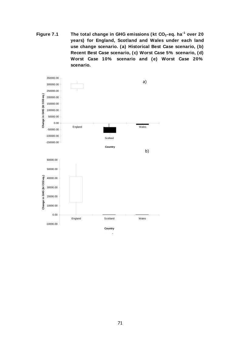
71

Figure 7.1 The total change in GHG emissions (kt CO2-eq. ha-1 over 20 years) for England, Scotland and Wales under each land use change scenario. (a) Historical Best Case scenario, (b) Recent Best Case scenario, (c) Worst Case 5% scenario, (d) Worst Case 10% scenario and (e) Worst Case 20% scenario.

-150000.00

-100000.00

-50000.00

0.00

50000.00

100000.00

150000.00

200000.00

250000.00

300000.00

350000.00

England Scotland Wales

Country

Cha

nge

in G

HG (k

t CO

2-eq

.)

Scotland

-150000.00

-100000.00

-50000.00

0.00

50000.00

100000.00

150000.00

200000.00

250000.00

300000.00

350000.00


Country

Chan

ge in

GHG

(kt C

O2-

eq.)

-10000.00

0.00

10000.00

20000.00

30000.00

40000.00

50000.00

60000.00


Country

Cha

nge

in G

HG

(kt C

O2-

eq.)

a)

b)

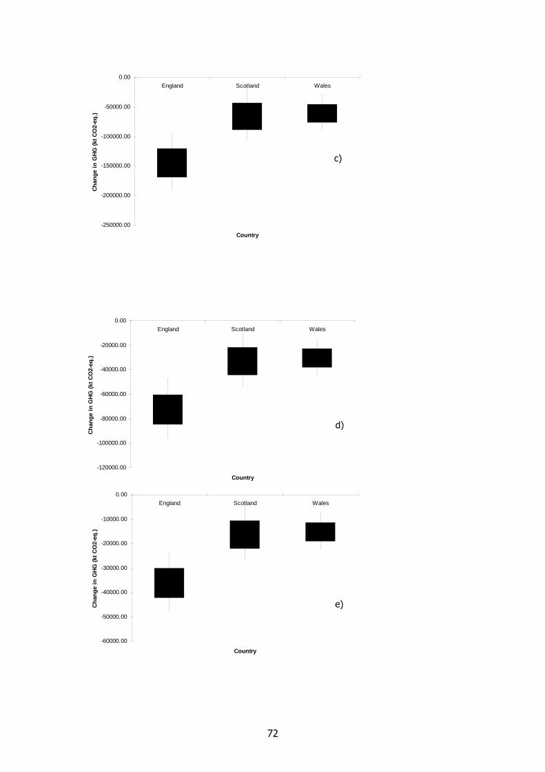
72

-250000.00

-200000.00

-150000.00

-100000.00

-50000.00

0.00England Scotland Wales

Country

Chan

ge in

GHG

(kt C

O2-

eq.)

-60000.00

-50000.00

-40000.00

-30000.00

-20000.00

-10000.00


Country

Cha

nge

in G

HG

(kt C

O2-

eq.)

-120000.00

-100000.00

-80000.00

-60000.00

-40000.00

-20000.00


Country

Chan

ge in

GHG

(kt C

O2-

eq.)

c)

d)

e)

73

Figure 7.2 The total change in GHG emissions (Mt CO2-eq. ha-1 over 20 years – estimates using the mean mitigation factor shown) for each county under each land use change scenario. (a) Historical Best Case scenario, (b) Recent Best Case scenario, (c) Worst Case 5% scenario, (d) Worst Case 10% scenario and (e) Worst Case 20% scenario.

a) b)

74

c) d)

75

e)

77

8 IMPLICATIONS OF THE FINDINGS

8.1 Overall implications

Land use change within the agricultural sector may not be a feasible large scale option for climate mitigation, with land use largely being determined by agricultural market conditions. Indeed, much of the potential global mitigation within this sector will be by changing management on land that remains in agricultural use (Smith et al. 2007c, 2008). We are therefore not proposing large scale land use change as a mitigation option, but instead have examined the consequences in terms of GHGs should land use change occur through other pressures.

The Historical Best Case scenario presents land use as it has been in the past (1930), but agricultural land use is not considered likely to return to conditions similar to these in the near future. We included this scenario as it presents a real case of land use for Great Britain, to show what SOC stocks/GHG emissions would have been under such circumstances. However, the historical best case for Great Britain as a whole is clearly not a “best case” for Scotland in terms of GHG emissions/SOC storage, with SOC storage higher in the baseline. The Recent Best Case scenario is probably closer to what could feasibly be achieved in the near term, but it only has a significant impact in England, with no significant impact in Wales or Scotland. Even for England, the impact is an order of magnitude lower than that of the historical best case scenario. Conversion of cropland to grassland is not a feasible mitigation option if a) there is no market incentive to convert (i.e. demand for livestock products derived from the grassland), or b) cropland area increases elsewhere to meet the demand for cropland products. In such a case, GHG emissions are simply displaced with no net GHG benefit (see Berry et al. 2008; Carlton et al. 2009, 2010). In any case, livestock emissions (from the new grassland if used to raise more livestock) would increase, thus negating at least some, if not all, of the GHG benefit.

The Worst Case scenarios, with 5, 10 and 20% plough out of permanent grassland, represent potential futures should cropland products (largely cereals in the UK) increase in market value to favour more crop production at the expense of grasslands, leading to a trade-off with grazed livestock production.

The Historical Best Case scenario delivers a Great Britain emission reduction of ~220 Mt CO2-eq. over 20 years, or an annual GHG emission reduction of ~11 Mt CO2-eq. yr-1 relative to the 2004 baseline. The Worst Case 20% grassland plough out scenario increases Great Britain emissions by a similar magnitude (-280 Mt CO2-eq. over 20 years; -14 Mt CO2-eq. yr-1). In the context of overall UK GHG emissions (635 Mt CO2-eq. yr-1 in 2007; Committee on Climate Change 2010) the yearly reductions/increases examined here are small, accounting for <2% of yearly annual GHG emissions, even for the most extreme scenario (Worst Case 20%). However, in the context of current UK

78

Land Use, Land-Use Change and Forestry (LULUCF) emissions, the changes in GHG emissions examined here are considerable. The Recent Best Case scenario would deliver further emission reductions (-1.4 Mt CO2-eq. yr-1), whereas even limited grassland plough out would result in an increase of emissions of around 3.5 Mt CO2-eq. yr-1.

8.2 Conclusions

Changes between agricultural land uses (transitions between permanent and temporary grassland and cropland) in Great Britain are likely to be a limited option for GHG mitigation, as land use is largely determined by market factors for agricultural products, and the suitability of the land. However, the impact of even relatively small agricultural land use change in Great Britain could have a significant impact in comparison with the current estimates of GHG emissions from land. In comparison with total UK GHG emissions, however, even the most extreme feasible land use change scenarios account for <2% of current emissions.

An assessment of soil profile carbon stocks in organic-mineral soils and salt marsh soils has established that salt marshes contribute <0.59% to the UK’s total soil carbon stock, although these soils could be sequestering C at relatively fast rates compared to other soil types, and at higher rates than previously estimated. With respect to GWP, salt marsh soils appear to remain relatively small sources of N2O which could be further reduced through reductions in nutrient enrichment.

8.3 Possible future work

This project has found that there is the need to improve access to soil datasets in the UK. Without this access there will remain areas of controversy, contention, disagreement, and obfuscation.

Refinement of the existing model could also be achieved through accounting for additional DOC fluxes by resolving issues of data quality, suitability, coverage, format and gaps in availability, as discussed particularly in the sections on Tasks 2 and 3. The Environment Agency and SEPA are increasing the amount of monitoring of dissolved organic carbon in freshwater in line with drivers from the Water Framework Directive. These data could resolve some of the outstanding issues cited above.

There is likely to be greater benefit in terms of the predictive capacity of any decision tool, from the examination of the effects of changes in land management as opposed to land use change. In particular, this may relate to fertilizer use or stocking density and cultivation practice.

There is a need for more measurement of changes in C stocks (to depth) following arable reversion to permanent grassland and also in ley-arable rotations. At present the lack of UK data means that it is very unclear how much of the C stored by rotational

79

grass is “lost” when that grassland is ploughed out. Informed assumptions on this have been made in line with the restrictions of the current datasets, but uncertainties are significant.

Subsoil C is also an issue. Most datasets look at the topsoil only and therefore do not account for the carbon in the subsoil. Many studies claim a benefit of reduced tillage, but only measure the topsoil. When the subsoil is included the benefit often disappears. Target studies to examine the behaviour of subsoil carbon under a range of tillage regimes would improve estimates of changes in C stocks. This would provide a sound evidence-base for policy makers on which to recommend practices for C loss mitigation.

This project has clearly shown a need for improved estimates of the extent of UK salt marshes and the heterogeneity of soil types within salt marshes. This could be particularly focussed upon C sequestration. In addition, improved data on the characteristics of salt marsh soils to include depth of UK salt marsh soils, carbon content to depth, and measured bulk densities would greatly improve estimates of C stocks.

80

9 REFERENCES

Adam P. 1997. Geographical variation in British saltmarsh vegetation. Journal of Ecology 66:339–366.

Alexander RB, Slack JR, Ludtke AS, Fitzgerald KK, Schertz TL. 1998. Data from selected U.S. Geological Survey national stream water-quality monitoring networks. Water Resour Res 34:2401-2405.

Anon. 1968. A century of agricultural statistics; Great Britain, 1866-1966. Ministry of Agriculture, Fisheries and Food, London, UK.

Avery BW. 1980. Soil classification for England and Wales (higher categories). Soil Survey Technical Monograph No. 14. Harpenden, UK.

Ball DF. 1964. Loss-on-ignition as an estimate of organic matter and organic carbon in non-calcareous soils. J Soil Sci 15:84–91.

Barker T, Bashmakov I, Bernstein L, Bogner J, Bosch P, Dave R, Davidson O, Fisher B, Grubb M, Gupta S, Halsnaes K, Heij B, Kahn Ribeiro S, Kobayashi S, Levine M, Martino D, Masera Cerutti O, Metz B, Meyer L, Nabuurs G-J, Najam A, Nakicenovic N, Rogner H-H, Roy J, Sathaye J, Schock R, Shukla P, Sims R, Smith P, Swart R, Tirpak D, Urge-Vorsatz D, Zhou D. 2007. Summary for policy makers. In: Metz B, Davidson OR, Bosch PR, Dave R, Meyer LA (Eds.), Climate change 2007: Mitigation. Contribution of Working group III to the Fourth Assessment Report of the Intergovernmental Panel on Climate Change, Cambridge University Press, Cambridge, United Kingdom and New York, NY, USA.

Barnes J, Owens NJP. 1998. Denitrification and nitrous oxide concentrations in the Humber estuary, UK, and adjacent coastal zones. Marine Pollution Bulletin 37:247-260.

Bellamy D, Wilkinson P. 2001. OSPAR 98/3: an environmental turning point or a flawed decision? Marine Pollution Bulletin 49:87-90.

Bellamy PH, Loveland PJ, Bradley RI, Lark RM, Kirk GJD. 2005. Carbon losses from all soils across England and Wales 1978-2003. Nature 437:245-248.

Berry PM, Kindred DR, Paveley ND. 2008. Quantifying the effects of fungicides and disease resistance on greenhouse gas emissions associated with wheat production. Plant Pathology 57:1000–1008.

Black HIJ, Booth P, Bellamy P, Elston D, Frogbrook ZL, Hudson G, Lark M, Potts J, Reynolds B. 2008. Design and operation of a UK Soil Monitoring Network. Defra, London.

Boorman LA. 2003. Saltmarsh review: an overview of coastal saltmarshes, their dynamic and sensitivity characteristics for conservation and management. JNCC Report No 334, Peterborough, UK.

Boorman LA, Hazelden JH, Loveland PJ, Wells JG. 1994. Comparative relationships between primary productivity and organic and nutrient fluxes in four salt marshes. In: Mitsch WJ (ed.) Global Wetlands: Old World and New. Amsterdam: Elsevier. pp 181-199.

Boorman DB, Hollis JM, Lilly A. 1995. Hydrology of soil types: a hydrological-based classification of the soils of the United Kingdom. Institute of Hydrology report no. 126, Wallingford, Oxon, UK.

Bradley RI, Milne R, Bell J, Lilly A, Jordan C, Higgins A. 2005. A soil carbon and land use database for the United Kingdom. Soil Use and Management 21:363-369.

Brew DS, Pye K. 2002. Guidance notes for assessing morphological changes in estuaries. Defra/Environment Agency Flood and Coastal Defence R&D Programme. Technical Report FD2110/TR1, London, UK.

Burd F. 1989. The salt marsh survey of Great Britain. An inventory of British salt marshes. Research and Survey in Nature Conservation No. 17, Nature Conservancy Council, Peterborough, UK.

Cannell MG, Milne R, Hargreaves KJ, Brown TA, Cruickshank MM, Bradley RI, Spencer T, Hope D, Billett MF, Adger WN, Subak S. 1999. National inventories of terrestrial carbon sources and sinks: the UK experience. Climate Change 42:505-530.

81

Carlton R, Berry P, Smith P. 2009. Investigating the interplay between UK crop yields, soil organic carbon stocks and greenhouse gas emissions. Aspects of Applied Biology 95:60-64.

Carlton R, Berry P, Smith P. 2010. Impact of crop yield reduction on GHG emissions from compensatory cultivation of pasture and forested land. International Journal of Agricultural Sustainability (in press).

Chmura GL, Anisfeld SC, Cahoon DR, Lynch JC. 2003. Global carbon sequestration in tidal, saline wetland soils. Global Biogeochemical Cycles 17:1-12.

Comber A, Procter C, Anthony S. 2008. The creation of a national agricultural land use dataset: combining pycnophylactic interpolation with dasymetric mapping techniques. Transactions in GIS 12:775-791.

Committee on Climate Change. 2010. UK and regions. Available at http://www.theccc.org.uk/topics/uk-and-regions. (Accessed 3rd February 2010).

Cundy AB, Croudace IW. 1996. Sediment accretion and recent sea-level rise in the Solent, Southern England: inferences from radiometric and geochemical studies. Estuary and Coastal Shelf Science 43:449–467.

Dankers N, Binsbergen M, Zegers K, Laane R, van der Loef M. 1984. Transport of water particulate and dissolved organic and inorganic matter between a salt marsh and the Ems Dollard estuary. Estuary and Coastal Shelf Science 19:143–165.

Dawson JJC, Smith P. 2007. Carbon losses from soil and its consequences for land management. Science of the Total Environment 382:165-190.

Defra and Environment Agency. 2005. Saltmarsh management manual http://www.saltmarshmanagementmanual.co.uk/Whatissaltmarsh.htm (accessed online 2010).

Dent DL, Downing EJ, Rogaar HR. 1976. Changes in the structure of marsh soil following drainage and arable cultivation. Journal of Soil Science 27:250-265.

De Vries A, Klavers HC. 1994. Riverine fluxes of pollutants: monitoring strategies first, calculation methods second. Eur Water Polln Contr 4:12-17.

Emmett BA, Reynolds B, Chamberlain PM, Rowe E, Spurgeon D, Brittain SA, Frogbrook Z, Hughes S, Lawlor AJ, Poskitt J, Potter E, Robinson DA, Scott A, Wood C, Woods C. 2010. Soils Report from 2007.CS Technical Report No. 9/07. Centre for Ecology & Hydrology. (Natural Environment Research Council), Wallingford, UK.

French JR. 1993. Numerical simulation of vertical marsh growth and adjustment to accelerated sea level rise, North Norfolk, UK. Earth Surface Processes and Landforms 18:63–81.

Guo LB, Gifford RM. 2002. Soil carbon stocks and land use change: a meta analysis. Global Change Biology 8:345-360.

Gustard A, Bullock A, Dixon J. 1992. Low flow estimation in the United Kingdom. IH Report 108, Wallingford, UK.

Hazelden LA. Boorman J. 2001. Soils and managed retreat in South East England. Soil Use and Management 17:150-154.

Hazelden J, Loveland PJ, Sturdy RG. 1986. Saline soils in North Kent. Soil Survey Special Survey No.14, Harpenden, UK.

Hodgson JM. 1997. Soil survey field handbook: describing and sampling soil profiles, 3rd Edition. Soil Survey Technical Monograph No. 5. Soil Survey and Land Research Centre, Silsoe, UK.

Holden J, Chapman P, Evans M, Hubacek K, Kay P, Warburton J. 2007. Vulnerability of organic soils in England and Wales. Final technical report to DEFRA and Countryside Council for Wales DEFRA Project SP0532/CCW contract FC 73-03-275. London, UK.

Howard PJA, Loveland PJ, Bradley RI, Dry FT, Howard DM, Howard DC. 1995. The carbon content of soil and its geographical distribution in Great Britain. Soil Use and Management 11:9-15.

IPCC. 1997. IPCC 1996 revised good practice guidelines for greenhouse gas inventories. Intergovernmental Panel on Climate Change (IPCC), Institute for Global Environmental Strategies, Tokyo, Japan.

82

IPCC. 2006. IPCC 2006 Revised good practice guidelines for greenhouse gas inventories. Intergovernmental Panel on Climate Change (IPCC), Institute for Global Environmental Strategies, Tokyo, Japan.

Jenkinson DS. 1990. The turnover of organic carbon and nitrogen in soil. Philosophical Transactions of the Royal Society, London B 329:361-368.

JNCC. 2005. Coastal salt marsh habitat action plan. Reporting status and reporting trends http://www.ukbap.org.uk/UKPlans.aspx?ID=33. Accessed October 2009.

Johnston AE. 1973. The effects of ley and arable cropping systems on the amounts of soil organic matter in the Rothamsted and Woburn Ley-Arable Experiments. Rothamsted Report for 1972, Part 2, 131-159.

Kenny C, Yamulki S, Blackwell M, Maltby E, French P, Birgand F. 2004. The release of nitrous oxide from the intertidal zones of two European estuaries in response to increased ammonium and nitrate loading. Water, Air, & Soil Pollution 4:61-66.

Laffoley Dd’A, Grimsditch G (eds.). 2009. The management of natural coastal carbon sinks. International Union for the Conservation of Nature, Gland, Switzerland. 53 pp.

Lilly A, Ball B, McTaggart I, DeGroote J. 2009a. Spatial modelling of nitrous oxide emissions at the national scale by upscaling using soil, climate and land use information. Global Change Biology 15:2321-2332.

Lilly A, Grieve IC, Jordan C, Baggaley NJ, Birnie RV, Futter MN, Higgins A, Hough R, Jones M, Noland AJ, Stutter MI, Towers W. 2009b. Climate change, land management and erosion in the organic and organic-mineral soils in Scotland and Northern Ireland. Scottish Natural Heritage Commissioned Report No.325 (ROAME No. F06AC104 - SNIFFER UKCC21). Inverness, UK

Lilly A, Bell JS, Hudson G, Nolan AJ, Towers W. 2010. National Soil Inventory of Scotland 1 (NSIS 1): Site location, sampling and profile description protocols (1978-1988). Technical Bulletin, Macaulay Institute, Aberdeen, UK.

Littlewood IG, Watts CD, Custance JM. 1998. Systematic application of United Kingdom river flow and quality databases for estimating annual river mass loads (1975 – 1994). Science of the Total Environment 210:21-40.

Loveland PJ, Hazelden J, Sturdy RG, Hodgson JM. 1986. Salt-affected soils in England and Wales. Soil Use and Management 2:150–156.

Loveland P, Bradley RI, Webb J, Jackson R, Black HIJ, Lane A. 2002. Comparison of soil data from different sources. Report of the comparison of the National Soil Inventory, the Representative Soil Sampling Scheme, The Countryside Survey 2000 soil sampling scheme and the Environmental Change network soil protocol. February 2002. MAFF/DEFRA Contract SP0515, London, UK.

McGrath SP, Loveland PJ. 1992. The soil geochemical atlas of England and Wales. Blackie Academic and Professional, Glasgow, UK.

Mudda SM, Howell SM, Morris JT. 2009. Impact of dynamic feedbacks between sedimentation, sea-level rise, and biomass production on near-surface marsh stratigraphy and carbon accumulation. Estuarine, Coastal and Shelf Science 82:377–389.

Ostle NJ, Levy PE, Evans CD, Smith P. 2009. UK land use and soil carbon sequestration. Land Use Policy 26 (Supplement 1) S274-S283. Elsevier, NL.

Pomeroy LR, Bancroft K, Breed J, Christian RR, Frankenberg D, Hall JR, Maurer LG, Wiebe WJ, Wiegert RG, Wetzel RL. 1977. Flux of organic matter through a salt marsh. Estuarine processes. In: Circulation, sediments and transfer of material in the estuary, vol. 2. Academic Press, USA, pp. 270–279.

Pye K, French PW. 1993. Erosion and accretion processes of British salt marshes, Vols. 2 and 3. Report to the UK Ministry of Agriculture, Fisheries and Food. Contract No. CSA1976, London, UK.

Shiel RS, Rimmer DL. 1984a. Changes in the soil structure and biological activity on some meadow hay plots at Cockle Park, Northumberland. Plant and Soil 76: 349–356.

83

SI. 1998. The action programme for nitrate vulnerable zones (England and Wales) Regulations, 1998. SI 1998/1202. The Stationary Office, London.

Simas T, Nunes JP, Ferreira JG. 2001. Effects of global climate change on coastal salt marshes. Ecological Modelling 139:1–15.

Smith P, Powlson DS, Smith JU, Falloon PD, Coleman K. 2000a. Meeting Europe’s climate change commitments: quantitative estimates of the potential for carbon mitigation by agriculture. Global Change Biology 6:525-539.

Smith P, Milne R, Powlson DS, Smith JU, Falloon PD, Coleman K. 2000b. Revised estimates of the carbon mitigation potential of UK agricultural land. Soil Use and Management 16:293-295.

Smith P, Goulding KW, Smith KA, Powlson DS, Smith JU, Falloon PD, Coleman K. 2000c. Including trace gas fluxes in estimates of the carbon mitigation potential of UK agricultural land. Soil Use and Management 16:251-259.

Smith P, Chapman SJ, Scott WA, Black HIJ, Wattenbach M, Milne R, Campbell C, Lilly A, Ostle N, Levy PE, Lumsdon DG, Millard P, Towers W, Zaehle S, Smith J. 2007a. Climate change cannot be entirely responsible for soil carbon loss observed in England and Wales, 1978 – 2003. Global Change Biology 13:2605-2609.

Smith JU, Chapman SJ, Bell JS, Bellarby J, Gottschalk P, Hudson G, Lilly A, Smith P, Towers W. 2007b. Developing a methodology to improve soil C stock estimates for Scotland and use of initial results from a resampling of the National Soil Inventory of Scotland to improve the Ecosse Model: Final Report. Rural and Environment Research and Analysis Directorate of the Scottish Government, Science Policy and Co-ordination Division, Edinburgh, UK.

Smith P, Smith J, Flyn H, Killham K, Rangel-Castro I, Foereid B, Aitkenhead M, Chapman S, Towers W, Bell J, Lumsdon D, Milne R, Thomson A, Simmons I, Skiba U, Reynolds B, Evans C, Frogbrook Z, Bradley I, Whitmore A. 2007. ECOSSE - Estimating carbon in organic soils sequestration and emissions. Report to Scottish Executive Environment and Rural Affairs Department, Edinburgh, UK. 177pp.

Smith JU, Chapman SJ, Bell J, Bellarby J, Gottschalk P, Hudson G, Lilly A, Smith P, Towers W. 2009. ECOSSE2. Developing a methodology to improve soil C stock estimates for Scotland and use of initial results from a resampling of the National Soil Inventory of Scotland to improve the Ecosse model., Report to Scottish Government on Project UAB-015-07. Edinburgh, UK.

Smith P, Martino D, Cai Z, Gwary D, Janzen H, Pushpam K, McCarl B, Ogle S, O’Mara S, Rice C, Scholes B, Sirotenko O, Howden M, McAllister T, Pan G, Romanenkov V, Schneider U, Towprayoon S, Wattenbach M, Smith J. 2008. Greenhouse gas mitigation in agriculture. Philosophical Transactions of the Royal Society B. 363:789-813.

Smith P, Gregory P, van Vuuren D, Obersteiner M, Rounsevell M, Woods J, Havlik P, Bellarby J. 2010. Competition for land. Philosophical Transactions of the Royal Society, B. (in review).

Sozanska M, Skiba U, Metcalfe S. 2002. Developing an inventory of N2O emissions from British Soils. Atmospheric Environment 36:987–998.

Tappin AD, Harris JRW, Uncles RJ. 2003. The fluxes and transformations of suspended particles, carbon and nitrogen in the Humber Estuary (UK) from 1994 to 1996: results from an integrated observation and modelling study. The Science of the Total Environment 314/316:665-713.

Tomlinson RW, Milne RM. 2006. Soil carbon stocks and land cover in Northern Ireland from 1939 to 2000. Applied Geography 26:18-39.

Worrall F, Burt TP, Adamson JK. 2006. The rate of and controls upon DOC loss in a peat catchment. Journal of Hydrology 321:311-325.

Worrall F, Burt TP. 2007. Flux of dissolved organic carbon from UK rivers. Global Biogeochemical Cycles 21: reference GB1013.

Worrall F, Guillbert T, Besien T. 2007. The flux of carbon from rivers: the case for flux from England and Wales. Biogeochemistry 86:63-75.

Worrall F, Burt TP, Rowson JG, Warburton J, Adamson JK. 2009. The multi-annual carbon budget of a peat-covered catchment. The Science of the Total Environment 407:4084-4094.

SP0567 Final report - GOV.UK

Documents

Transcript of SP0567 Final report - GOV.UK