Sources, Exposure and Exposure Assessment - IARC Monographs

1. Sources, Exposure and Exposure Assessment

1.1 Sources

1.1.1 Natural magnetic and electric fields

Humans are exposed daily to electric and magnetic fields from both natural andman-made sources. The strengths of fields from man-made sources can exceed thosefrom natural sources by several orders of magnitude.

The existence of the geomagnetic field has been known since ancient times. Thegeomagnetic field is primarily dipolar in nature. The total field intensity diminishesfrom its maxima of about 60 μT at the magnetic poles, to a minimum of about 30 μTnear the equator (König et al., 1981). In temperate latitudes, the geomagnetic field, atsea-level, is approximately 45–50 μT whereas in regions of southern Brazil, fluxdensities as low as 24 μT have been reported (Hansson Mild, 2000).

The geomagnetic field is not constant but fluctuates continuously and is subject todiurnal, lunar and seasonal variations (Strahler, 1963; König et al., 1981). Moreinformation on this subject is available (Dubrov, 1978) and in databases on the Web(e.g. National Geophysical Data Center).

There are also short-term variations associated with ionospheric processes. When thesolar wind carries protons and electrons towards the earth, phenomena such as theNorthern Lights, and rapid fluctuations in the intensity of the geomagnetic field occur.Figure 1 shows a 9-hour recording made at the Kiruna observatory in Sweden in January2002. The variation may be large and can sometimes range from 0.1 μT to 1 μT withina few minutes. Such rapid variations are rare and correlated with the solar cycle. Morecommonly, variations of similar magnitude occur over a longer period of time. Despitethese variations, the geomagnetic field should always be considered as a static field.

The atmosphere also has an electric field that is directed radially because the earthis negatively charged. The field strength depends to some extent on geographicallatitude; it is lowest towards the poles and the equator and highest in the temperatelatitudes. The average strength is around 100 V/m in fair weather, although it may rangefrom 50–500 V/m depending on weather, altitude, time of day and season. Duringprecipitation and bad weather, the values can change considerably, varying over a rangeof ± 40 000 V/m (König et al., 1981). The average atmospheric electric field is not verydifferent from that produced in most dwellings by typical 50- or 60-Hz electric field

–51–

power sources (National Radiological Protection Board, 2001), except when measure-ments are made very close to electric appliances.

The electromagnetic processes associated with lightning discharges are termedatmospherics or ‘sferics’ for short. They occur in the ELF range and at higherfrequencies (König et al., 1981). Each second, about 100 lightning discharges occurworldwide and can be detected thousands of kilometres away (Hansson Mild, 2000).

1.1.2 Man-made fields and exposure

People are exposed to electric and magnetic fields arising from a wide variety ofsources which use electrical energy at various frequencies. Man-made sources are thedominant sources of exposure to time-varying fields. At power frequencies (a term thatencompasses 50 and 60 Hz and their harmonics), man-made fields are many thousandsof times greater than natural fields arising from either the sun or the earth.

When the source is spatially fixed and the source current and/or electrical potentialdifference is constant in time, the resulting field is also constant, and is referred to asstatic, hence the terms magnetostatic and electrostatic. Electrostatic fields are producedby fixed potential differences. Magnetostatic fields are established by permanentmagnets and by steady currents. When the source current or voltage varies in time, forexample, in a sinusoidal, pulsed or transient manner, the field varies proportionally.

IARC MONOGRAPHS VOLUME 8052

Figure 1. Magnetogram recording from a geomagnetic research station in Kiruna,Sweden

Kiruna magnetogram 2002-01-28, 09:13:35Real-time geomagnetogram recordings can be seen at (http://www.irf.se/mag). The recordings are made inthree axes: X, north, Y, east, and Z, down. The trace shown is the deflection from the mean value of themagnetic field at this location.

In practice, the waveform may be a simple sinusoid or may be more complex,indicating the presence of harmonics. Complex waveforms are also observed whentransients occur. Transients and interruptions, either in the electric power source or inthe load, result in a wide spectrum of frequencies that may extend above several kHz(Portier & Wolfe, 1998).

Power-frequency electric and magnetic fields are ubiquitous and it is important toconsider the possibilities of exposure both at work and at home. Epidemiologicalstudies may focus on particular populations because of their proximity to specificsources of exposure, such as local power lines and substations, or because of their useof electrical appliances. These sources of exposure are not necessarily the dominantcontributors to a person’s time-weighted average exposure if this is indeed theparameter of interest for such studies. Various other metrics have been proposed thatreflect aspects of the intermittent and transient characteristics of fields. Man-madesources and their associated fields are discussed more fully elsewhere (see NationalRadiological Protection Board, 2001).

(a) Residential exposureThere are three major sources of ELF electric and magnetic fields in homes:

multiple grounded current-carrying plumbing and/or electric circuits, appliances andnearby power lines, including lines supplying electricity to individual homes (knownas service lines, service drops or drop lines).

(i) Background exposureExtremely low-frequency magnetic fields in homes arise mostly from currents

flowing in the distribution circuits, conducting pipes and the electric ground, and fromthe use of appliances. The magnetic fields are partially cancelled if the load currentmatches the current returning via the neutral conductor. The cancellation is moreeffective if the conductors are close together or twisted. In practice, return currents donot flow exclusively through the associated neutral cable, but are able to follow alter-native routes because of interconnected neutral cables and multiple earthing of neutralconductors. This diversion of current from the neutral cable associated with a particularphase cable results in unbalanced currents producing a net current that gives rise to aresidual magnetic field. These fields produce the general background level inside andoutside homes (National Radiological Protection Board, 2001). The magnetic fields inthe home that arise from conductive plumbing paths were noted by Wertheimer et al.(1995) to “provide opportunity for frequent, prolonged encounters with ‘hot spots’ ofunusually high intensity field — often much higher than the intensity cut-points around[0.2 or 0.3 μT] previously explored”.

The background fields in homes have been measured in many studies. Swansonand Kaune (1999) reviewed 27 papers available up to 1997; other significant studieshave been reported by Dockerty et al. (1998), Zaffanella and Kalton (1998), McBrideet al. (1999), UK Childhood Cancer Study Investigators (UKCCSI) (1999) and Schüz

SOURCES, EXPOSURE AND EXPOSURE ASSESSMENT 53

et al. (2000). The distribution of background field intensities in a population is usuallybest characterized by a log-normal distribution. The mean field varies from country tocountry, as a consequence of differences in supply voltages, per-capita electricity con-sumption and wiring practices, particularly those relating to earthing of the neutral.Swanson and Kaune (1999) found that the distribution of background fields, measuredover 24 h or longer, in the USA has a geometric mean of 0.06–0.07 μT, correspondingto an arithmetic mean of around 0.11 μT, and that fields in the United Kingdom arelower (geometric mean, 0.036–0.039 μT; arithmetic mean, approximately 0.05 μT), butfound insufficient studies to draw firm conclusions on average fields in other Europeancountries. Wiring practices in some countries such as Norway lead to particularly lowfield strengths in dwellings (Hansson Mild et al., 1996).

In addition to average background fields, there is interest in the percentages ofhomes with fields above various cut-points. Table 1 gives the magnetic field strengthsmeasured over 24 or 48 h in the homes of control subjects from four recent large epi-demiological studies of children.

Few homes are exposed to significant fields from high-voltage power lines (seebelow). Even in homes with fields greater than 0.2 or 0.4 μT, high-voltage power linesare not the commonest source of the field.

The electric field strength measured in the centre of a room is generally in the range1–20 V/m. Close to domestic appliances and cables, the field strength may increase toa few hundred volts per metre (National Radiological Protection Board, 2001).


Table 1. Measured exposure to magnetic fields in residential epi-demiological studies

Percentage ofcontrols exposedto field strengthsgreater than

Study Country No. of controlchildren havinglong-termmeasurements

0.2 μT 0.4 μT

Linet et al. (1997)a USA 530 9.2 0.9McBride et al. (1999)a Canada 304 11.8 3.3UKCCSI (1999)a United Kingdom 2224 1.5 0.4Schüz et al. (2001a)b Germany 1301 1.4 0.2

UKCCSI, UK Childhood Cancer Study Investigatorsa Percentages calculated from data on geometric means from Ahlbom et al. (2000). (Theresults presented by Dockerty et al. (1999) have not been included as the numbers aretoo small to be meaningful at these field strengths.)b Percentages calculated from medians from original data. The medians are expected tobe very similar to the geometric means.

(ii) Fields from appliancesThe highest magnetic flux densities to which most people are exposed in the home

arise close to domestic appliances that incorporate motors, transformers and heaters(for most people, the highest fields experienced from domestic appliances are alsohigher than fields experienced at work and outside the home). The flux densitydecreases rapidly with distance from appliances, varying between the inverse squareand inverse cube of distance, and at a distance of 1 m the flux density will usually besimilar to background levels. At a distance of 3 cm, magnetic flux densities may beseveral hundred microtesla or may even approach 2 mT from devices such as hairdryers and can openers, although there can be wide variations in fields at the samedistance from similar appliances (National Radiological Protection Board, 2001).

Exposure to magnetic fields from home appliances must be considered separatelyfrom exposure to fields due to power lines. Power lines produce relatively low-intensity, small-gradient fields that are always present throughout the home, whereasfields produced by appliances are invariably more intense, have much steepergradients, and are, for the most part, experienced only sporadically. The appropriateway of combining the two field types into a single measure of exposure dependscritically on the exposure metric considered.

Various features of appliances determine their potential to make a significantcontribution to the fields to which people are exposed, and epidemiological studies ofappliances have focused on particular appliances chosen for the following reasons:

• Use particularly close to or touching the body. Examples include hair dryers,electric shavers, electric drills and saws, and electric can openers or foodmixers.

• Use at moderately close distances for extended periods of time. Examplesinclude televisions and video games, sewing machines, bedside clocks andclock radios and night storage heaters, if, for example, they are located close tothe bed.

• Use while in bed, combining close proximity with extended periods of use.Examples include electric blankets and water beds (which may or may not beleft on overnight).

• Use over a large part of the home. Examples include underfloor electricheating.

Table 2 gives values of broadband magnetic fields at various distances fromdomestic appliances in use in the United Kingdom (Preece et al., 1997). The magneticfields were calculated from a mathematical model fitted to actual measurements madeon the numbers of appliances shown in the Table. Gauger (1985) and Zaffanella &Kalton (1998) reported narrow band and broadband data, respectively, for the USA.Florig and Hoburg (1990) characterized fields from electric blankets, using a three-dimensional computer model and Wilson et al. (1996) used spot measurements made inthe home and in the laboratory. They reported that the average magnetic fields to which



Table 2. Resultant broadband magnetic field calculated at 5, 50 and 100 cmfrom appliances for which valid data could be derived on the basis ofmeasured fields at 5, 30, 60 and 100 cm

Magnetic field (μT) at discrete distances from the surface of appliancescomputed from direct measurements

Appliance type No. 5 cm ± SD 50 cm ± SD 100 cm ± SD

Television 73 2.69 1.08 0.26 0.11 0.07 0.04Kettle, electric 49 2.82 1.51 0.05 0.06 0.01 0.02Video-cassette recorder 42 0.57 0.52 0.06 0.05 0.02 0.02Vacuum cleaner 42 39.53 74.58 0.78 0.74 0.16 0.12Hair dryer 39 17.44 15.56 0.12 0.10 0.02 0.02Microwave oven 34 27.25 16.74 1.66 0.63 0.37 0.14Washing machine 34 7.73 7.03 0.96 0.56 0.27 0.14Iron 33 1.84 1.21 0.03 0.02 0.01 0.00Clock radio 32 2.34 1.96 0.05 0.05 0.01 0.01Hi-fi system 30 1.56 4.29 0.08 0.14 0.02 0.03Toaster 29 5.06 2.71 0.09 0.08 0.02 0.02Central heating boiler 26 7.37 10.10 0.27 0.26 0.06 0.05Central heating timer 24 5.27 7.05 0.14 0.17 0.03 0.04Fridge/freezer 23 0.21 0.14 0.05 0.03 0.02 0.01Radio 23 3.00 3.26 0.06 0.04 0.01 0.01Central heating pump 21 61.09 59.58 0.51 0.47 0.10 0.10Cooker 18 2.27 1.33 0.21 0.15 0.06 0.04Dishwasher 13 5.93 4.99 0.80 0.46 0.23 0.13Freezer 13 0.42 0.87 0.04 0.02 0.01 0.01Oven 13 1.79 0.89 0.39 0.23 0.13 0.09Shower, electric 12 30.82 35.04 0.44 0.75 0.11 0.25Burglar alarm 10 6.20 5.21 0.18 0.11 0.03 0.02Food processor 10 12.84 12.84 0.23 0.23 0.04 0.04Extractor fan 9 45.18 107.96 0.50 0.93 0.08 0.14Cooker hood 9 4.77 2.53 0.26 0.10 0.06 0.02Speaker 8 0.48 0.67 0.07 0.13 0.02 0.04Hand blender 8 76.75 87.09 0.97 1.05 0.15 0.16Tumble dryer 7 3.93 5.45 0.34 0.42 0.10 0.10Food mixer 6 69.91 69.91 0.69 0.69 0.11 0.11Fish-tank pump 6 75.58 64.74 0.32 0.09 0.05 0.01Computer 6 1.82 1.96 0.14 0.07 0.04 0.02Electric clock 6 5.00 4.15 0.04 0.00 0.01 0.00Electric knife 5 27.03 13.88 0.12 0.05 0.02 0.01Hob 5 2.25 2.57 0.08 0.05 0.01 0.01Deep-fat fryer 4 4.44 1.99 0.07 0.01 0.01 0.00Tin/can opener 3 145.70 106.23 1.33 1.33 0.20 0.21Fluorescent light 3 5.87 8.52 0.15 0.20 0.03 0.03Fan heater 3 3.64 1.41 0.22 0.18 0.06 0.06Liquidizer 2 3.28 1.19 0.29 0.35 0.09 0.12

the whole body is exposed are between 1 and 3 μT. From eight-hour measurements, Leeet al. (2000) estimated that the time-weighted average magnetic field exposures fromovernight use of electric blankets ranged between 0.1 and 2 μT.

Measurements of personal exposure are expected to be higher than measurementsof background fields because they include exposures from sources such as appliances.Swanson and Kaune (1999) found that in seven studies which measured personalexposure and background fields for the same subjects, the ratio varied from 1.0 to 2.3with an average of 1.4.

(iii) Power linesPower lines operate at voltages ranging from the domestic supply voltage (120 V

in North America, 220–240 V in Europe) up to 765 kV in high-voltage power lines(WHO, 1984). At higher voltages, the main source of magnetic field is the load currentcarried by the line. Higher voltage lines are usually also capable of carrying highercurrents. As the voltage of the line and, hence, in general, the current carried, and theseparation of the conductors decrease, the load current becomes a progressively lessimportant source of field and the net current, as discussed in (i) above, becomes thedominant source. It is therefore convenient to treat high-voltage power lines (usuallytaken to mean 100 kV or 132 kV, also referred to as transmission lines) as a separatesource of field (Merchant et al., 1994; Swanson, 1999).

High-voltage power lines in different countries follow similar principles, but withdifferences in detail so that the fields produced are not identical (power-line design asit affects the fields produced was reviewed by Maddock, 1992). For example, high-voltage power lines in the United Kingdom can have lower ground clearances and cancarry higher currents than those in some other countries, leading to higher fields underthe lines. When power lines carry two or more circuits, there is a choice as to thephysical distribution of the various wires on the towers. An arrangement called‘transposed phasing’, in which the wires or bundles of wire — phases — in the circuit


Table 2 (contd)

Magnetic field (μT) at discrete distances from the surface of appliancescomputed from direct measurements

Appliance type No. 5 cm ± SD 50 cm ± SD 100 cm ± SD

Bottle sterilizer 2 0.41 0.17 0.01 0.00 0.00 0.00Coffee maker 2 0.57 0.03 0.06 0.07 0.02 0.02Shaver socket 2 16.60 1.24 0.27 0.01 0.04 0.00Coffee mill 1 2.47 0.28 0.07Shaver, electric 1 164.75 0.84 0.12Tape player 1 2.00 0.24 0.06

From Preece et al. (1997)

on one side of the tower have the opposite order to those on the other side, results infields that decrease more rapidly with distance from the lines than the alternatives(Maddock, 1992). Transposed phasing is more common in the United Kingdom than,for example, in the USA.

In normal operation, high-voltage power lines have higher ground clearances thanthe minimum permitted, and carry lower currents than the maximum theoreticallypossible. Therefore, the fields present in normal operation are substantially lower thanthe maxima theoretically possible.

Electric fields

High-voltage power lines give rise to the highest electric field strengths that arelikely to be encountered by people. The maximum unperturbed electric field strengthimmediately under 400-kV transmission lines is about 11 kV/m at the minimumclearance of 7.6 m, although people are generally exposed to fields well below thislevel. Figure 2 gives examples of the variation of electric field strength with distancefrom the centreline of high-voltage power lines with transposed phasing in the UnitedKingdom. At 25 m to either side of the line, the field strength is about 1 kV/m (NationalRadiological Protection Board, 2001).

Objects such as trees and other electrically grounded objects have a screening effectand generally reduce the strength of the electric fields in their vicinity. Buildingsattenuate electric fields considerably, and the electric field strength may be one to three


Figure 2. Electric fields from high-voltage overhead power lines

From National Radiological Protection Board (2001)

orders of magnitude less inside a building than outside it. Electric fields to which peopleare exposed inside buildings are generally produced by internal wiring and appliances,and not by external sources (National Radiological Protection Board, 2001).

Magnetic fields

The average magnetic flux density measured directly beneath overhead powerlines can reach 30 μT for 765-kV lines and 10 μT for the more common 380-kV lines(Repacholi & Greenebaum, 1999). Theoretical calculations of magnetic flux densitybeneath the highest voltage power line give ranges of up to 100 μT (NationalRadiological Protection Board, 2001). Figure 3 gives examples of the variation ofmagnetic flux density with distance from power lines in the United Kingdom.Currents (and hence the fields produced) vary greatly from line to line because powerconsumption varies with time and according to the area in which it is measured.

Magnetic fields generally fall to background strengths at distances of 50–300 mfrom high-voltage power lines depending on the line design, current and the strengthof background fields in the country concerned (Hansson Mild, 2000). Few people liveso close to high-voltage power lines (see Table 3); meaning that these power lines area major source of exposure for less than 1% of the population according to most studies(see Table 4).

In contrast to electric fields for which the highest exposure is likely to beexperienced close to high-voltage power lines, the highest magnetic flux densities are


Figure 3. Magnetic fields from high-voltage overhead power lines

From National Radiological Protection Board (2001)

more likely to be encountered in the vicinity of appliances or types of equipment thatcarry large currents (National Radiological Protection Board, 2001).

Direct current lines

Some high-voltage power lines have been designed to carry direct current (DC),therefore producing both electrostatic and magnetostatic fields. Under a 500-kV DCtransmission line, the static electric field can reach 30 kV/m or higher, while themagnetostatic field from the line can average 22 μT which adds vectorially to theearth’s field (Repacholi & Greenebaum, 1999).


Table 3. Percentages of people in certain countries within variousdistances of high-voltage power lines

Subjects withinthis distance

Country (reference) No. ofsubjects

Voltages ofpower linesincluded (kV)

Distance(m)

No. %

Canada (McBrideet al., 1999)

399a ≥ 50 50100

4 7

1.001.75

Denmark (Olsenet al., 1993)

6495b 132–15050–60

75 35

2822

0.430.340.46

50–440 150 52 0.80

United Kingdom(Swanson, 1999)

22 millionc ≥ 275 50100

0.070.21

United Kingdom(UKCCSI, 2000a)

3390a ≥ 66 50120

935

0.271.03

≥ 275 50120

3 9

0.090.27

USA (Kleinermanet al., 2000)

405a ≥ 50d

power linetransmissionline

40 40

9820

24.24.94

UKCCSI, UK Childhood Cancer Study Investigatorsa Controls from epidemiological study of childrenb Cases and controls from epidemiological study of childrenc All homes in England and Wales (Source: Department of Transport, Local Govern-ment and the Regions; National Assembly for Wales, 1998, http://www.statis-tics.gov.uk/statbase/Expodata/Spreadsheets/D4524.xls)d Not stated in Kleinerman et al. (2000), assumed to be the same as Wertheimer& Leeper (1979)

(iv) SubstationsOutdoor substations normally do not increase residential exposure to electric and

magnetic fields. However, substations inside buildings may result in exposure tomagnetic fields at distances less than 5–10 m from the stations (National RadiologicalProtection Board, 2001). On the floor above a station, flux densities of the order of10–30 μT may occur depending on the design of the substation (Hansson Mild et al.,1991). Normally, the main sources of field are the electrical connections (known asbusbars) between the transformer and the other parts of the substation. Thetransformer itself can also be a contributory source.

(v) Exposure to ELF electric and magnetic fields in schoolsExposure to ELF electric and magnetic fields while at school may represent a

significant fraction of a child’s total exposure. A study involving 79 schools in Canadatook a total of 43 009 measurements of 60-Hz magnetic fields (141–1543 per school).Only 7.8% of all the fields measured were above 0.2 μT. For individual schools, theaverage magnetic field was 0.08 μT (SD, 0.06 μT). In the analysis by use of room,only typing rooms had magnetic fields that were above 0.2 μT. Hallways and corridorswere above 0.1 μT and all other room types were below 0.1 μT. The percentage ofclassrooms above 0.2 μT was not reported. Magnetic fields above 0.2 μT were mostlyassociated with wires in the floor or ceiling, proximity to a room containing electricalappliances or movable sources of magnetic fields such as electric typewriters,


Table 4. Percentages of people in various countries living in homes inwhich high-voltage power lines produce magnetic fields in excess ofspecified values

Subjects whosehomes exceed themeasured field

Country (reference) No. ofsubjects

Voltages ofpower linesincluded (kV)

Measuredfield (μT)

No. %

Denmark (Olsenet al., 1993)

4788a ≥ 50 0.250.4

11 3

0.230.06

Germany (Schüzet al., 2000)

1835b ≥ 123 0.2 8 0.44

United Kingdom(UKCCSI, 2000a)

3390a ≥ 66c 0.20.4

11 8

0.320.24

UKCCSI, UK Childhood Cancer Study Investigatorsa Controls from epidemiological study of childrenb Cases and controls from epidemiological study of childrenc Probably over 95% were ≥ 132 kV

computers and overhead projectors. Eight of the 79 schools were situated near high-voltage power lines. The survey showed no clear difference in overall magnetic fieldstrength between the schools and domestic environments (Sun et al., 1995).

Kaune et al. (1994) measured power-frequency magnetic fields in homes and inthe schools and daycare centres of 29 children. Ten public shools, six private schoolsand one daycare centre were included in the study. In general, the magnetic fieldstrengths measured in schools and daycare centres were smaller and less variable thanthose measured in residential settings.

The UK Childhood Cancer Study Investigators (UKCCSI) (1999) carried out anepidemiological study of children in which measurements were made in schools aswell as homes. Only three of 4452 children aged 0–14 years who spent 15 or morehours per week at school during the winter, had an average exposure during the yearabove 0.2 μT as a result of exposure at school.

In a preliminary report reviewed elsewhere (Portier & Wolfe, 1998), Neutra et al.(1996) reported a median exposure level of 0.08 μT for 163 classrooms at sixCalifornia schools, with approximately 4% of the classrooms having an averagemagnetic field in excess of 0.2 μT. These fields were mainly due to ground currentson water pipes, with nearby distribution lines making a smaller contribution. [TheWorking Group noted that no primary publication was available.] The study wassubsequently extended and an executive summary was published in an electronicform, which is available at www.dhs.ca.gov/ehib/emf/school_exp_ass_exec.pdf

(b) Occupational exposureExposure to magnetic fields varies greatly across occupations. The use of personal

dosimeters has enabled exposure to be measured for particular types of job. Table 5(Portier & Wolfe, 1998) lists the time-weighted average exposure to magnetic fieldsfor selected job classifications. In some cases the standard deviations are large. Thisindicates that there are instances in which workers in these categories are exposed tofar stronger fields than the means listed here.

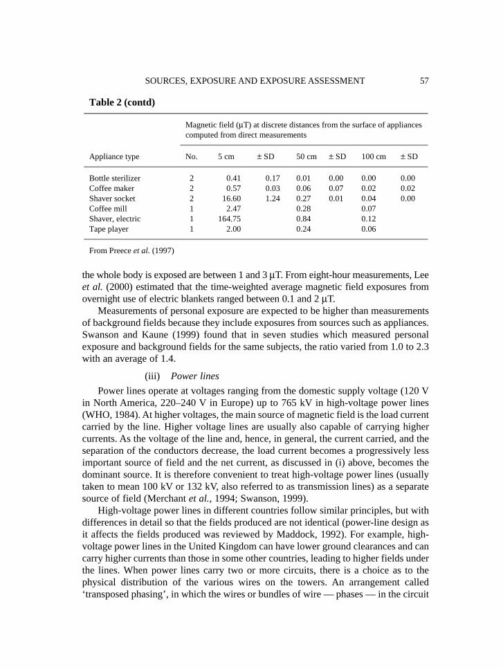
Floderus et al. (1993) investigated sets of measurements made at 1015 differentworkplaces using EMDEX (electric and magnetic field digital exposure system)-100and EMDEX-C personal dosimeters. This study covered 169 different job categoriesand participants wore the dosimeters for a mean duration of 6.8 h. The distribution ofall 1-s sampling period results for 1015 measurements is shown in Figure 4. The mostcommon measurement was 0.05 μT and measurements above 1 μT were rare. It shouldbe noted that the response of the EMDEX-C is non-linear over a wide frequencyrange. For example, the railway frequency in Sweden is 16 2/3 Hz, which means thatthe measurements obtained with the EMDEX are underestimates of the exposure.

It can be seen from Table 5 that workers in certain occupations are exposed toelevated magnetic fields. Some of the more significant occupations are consideredbelow.



Table 5. Time-weighted average exposure to magneticfields by job title

Occupational title Average exposure(μT)

Standard deviation

Train (railroad) driver 4.0 NRLineman 3.6 11Sewing machine user 3.0 0.3Logging worker 2.5 7.7Welder 2.0 4.0Electrician 1.6 1.6Power station operator 1.4 2.2Sheet metal worker 1.3 4.2Cinema projectionist 0.8 0.7

Modified from Portier & Wolfe (1998)NR, not reported

Modified from National Radiological Protection Board (2001) (original figure from Floderus et al., 1993)The distribution should not be interpreted as a distribution of results for individuals.

Figure 4. Distribution of all occupational magnetic field samples

(i) The electric power industryStrong magnetic fields are encountered mainly in close proximity to high currents

(Maddock, 1992). In the electric power industry, high currents are found in overheadlines and underground cables, and in busbars in power stations and substations. Thebusbars close to generators in power stations can carry currents up to 20 times higherthan those typically carried by the 400-kV transmission system (Merchant et al., 1994).

Exposure to the strong fields produced by these currents can occur either as a directresult of the job, e.g. a lineman or cable splicer, or as a result of work location, e.g.when office workers are located on a power station or substation site. It should be notedthat job categories may include workers with very different exposures, e.g. linemenworking on live or dead circuits. Therefore, although reporting magnetic-field exposureby job category is useful, a complete understanding of exposure requires a knowledgeof the activities or tasks and the location as well as measurements made by personalexposure meters.

The average magnetic fields to which workers are exposed for various jobs in theelectric power industry have been reported as follows: 0.18–1.72 μT for workers inpower stations, 0.8–1.4 μT for workers in substations, 0.03–4.57 μT for workers onlines and cables and 0.2–18.48 μT for electricians (Portier & Wolfe, 1998; NationalRadiological Protection Board, 2001).

(ii) Arc and spot weldingIn arc welding, metal parts are fused together by the energy of a plasma arc struck

between two electrodes or between one electrode and the metal to be welded. A power-frequency current usually produces the arc but higher frequencies may be used inaddition to strike or to maintain the arc. A feature of arc welding is that the weldingcable, which can carry currents of hundreds of amperes, can touch the body of theoperator. Stuchly and Lecuyer (1989) surveyed the exposure of arc welders tomagnetic fields and determined separately the exposure at 10 cm from the head, chest,waist, gonads, hands and legs. Whilst it is possible for the hand to be exposed to fieldsin excess of 1 mT, the trunk is typically exposed to several hundred microtesla. Oncethe arc has been struck, these welders work with comparatively low voltages and thisis reflected in the electric field strengths measured; i.e. up to a few tens of volts permetre (National Radiological Protection Board, 2001).

Bowman et al. (1988) measured exposure for a tungsten–inert gas welder of up to90 μT. Similar measurements reported by the National Radiological Protection Boardindicate magnetic flux densities of up to 100 μT close to the power supply, 1 mT at thesurface of the welding cable and at the surface of the power supply and 100–200 μTat the operator position (National Radiological Protection Board, 2001). London et al.(1994) reported the average workday exposure of 22 welders and flame cutters to bemuch lower (1.95 μT).


(iii) Induction furnacesMeasurements on induction furnaces and heaters operating in the frequency range

from 50 Hz to 10 kHz have been reported (Lövsund et al., 1982) and are summarizedin Table 6. The field strengths decrease rapidly with distance from the coils and do notreflect whole-body exposure. However, in some cases, whole-body exposure occurs.Induction heater operators experience short periods of exposure to relatively strongfields as the induction coils are approached (National Radiological Protection Board,2001).

(iv) Electrified transportElectricity is utilized in various ways in public transport. The power is supplied as

DC or at alternating frequencies up to those used for power distribution. ManyEuropean countries such as Austria, Germany, Norway, Sweden and Switzerland havesystems that operate at 16 2/3 Hz. Most of these systems use a DC traction motor, andrectification is carried out either on-board or prior to supply. On-board rectificationusually requires a smoothing inductor, a major source of static and 100-Hz alternatingmagnetic fields. For systems that are supplied with nominal DC there is littlesmoothing at the rectification stage, resulting in a significant alternating component inthe ‘static’ magnetic fields (National Radiological Protection Board, 2001).

On Swedish trains, Nordenson et al. (2001) found values ranging from 25 to120 μT for power-frequency fields in the driver’s cab, depending on the type (age andmodel) of locomotive. Typical daily average exposures were in the range of 2–15 μT.

Other forms of transport, such as aeroplanes and electrified road vehicles are alsoexpected to increase exposure, but have not been investigated extensively.


Table 6. Frequency and magnetic flux densities from induction furnaces

Type of machine No. Frequency band Magnetic fluxdensity (mT):measured ranges

Ladle furnace in conjunction with 1.6-Hz magnetic stirrer, measurements made at 0.5–1 m from furnace

1 1.6 Hz, 50 Hz 0.2–10

Induction furnace, at 0.6–0.9 m 2 50 Hz 0.1–0.9 at 0.8–2.0 m 5 600 Hz 0.1–0.9Channel furnace, at 0.6–3.0 m 3 50 Hz 0.1–0.4Induction heater, at 0.1–1.0 m 5 50 Hz–10 kHz 1–60

Modified from Lövsund et al. (1982)

(v) Use of video display terminalsOccupational exposure to ELF electric and magnetic fields from video display

terminals has recently received attention. Video display terminals produce both power-frequency fields and higher frequency fields ranging from about 50 Hz up to 50 kHz(Portier & Wolfe, 1998). Sandström et al. (1993) reported median magnetic fields atELF as 0.21 μT and 0.03 μT for frequencies between 15 kHz and 35 kHz. The medianelectric fields measured in the same frequency ranges were 20 V/m and 1.5 V/m,respectively.

(vi) Use of sewing machinesHansen et al. (2000) reported higher-than-background magnetic fields near

industrial sewing machines, because of proximity to motors, with field strengthsranging from 0.32–11.1 μT at a position corresponding approximately to the sternumof the operator. The average exposure for six workers working a full work-shift in thegarment industry ranged from 0.21–3.20 μT.

(c) TransientsTransients occur in electrical systems mainly as a result of switching loads or

circuits on and off. They can be produced deliberately, as in circuit testing, or occuraccidentally, caused by sudden changes in current load following a short-circuit orlightning strike. Such disturbances invariably have a much higher frequency contentthan that of the signal that is interrupted (Kaune et al., 2000).

A number of devices have been designed to record electric power transients(Deadman et al., 1988; Héroux, 1991; Kaune et al., 2000). These devices differ primarilyin the range of frequencies used to define a transient and in their storage capacities.Kaune et al. (2000) examined magnetic transients within the range of 2–200 kHz thathad threshold peak intensity levels, measured using a dual channel recorder, of either 3.3or 33 nT. Recordings were made for a minimum of 24 h in each of 156 homes distributedat six different locations in the USA. Although the recordings of the less intense 3.3-nTtransients might have been contaminated somewhat by nearby television sets, this wasnot the case for the recordings of the 33-nT transients. It was found that transient activityin homes has a distinct diurnal pattern, generally following variations in power use.Evidence was also presented indicating that the occurrence of the larger, 33-nT magnetictransients is increased (p = 0.01) in homes with well-grounded metal plumbing that isalso electrically connected to an external water system. In contrast, the increasedtransient activity in the homes tested was not related to wire code.


1.2 Instrumentation and computational methods of assessing electric andmagnetic fields

1.2.1 Instruments

Measurements of electric and magnetic fields are used to characterize emissionsfrom sources and exposure of persons or experimental subjects. The mechanisms thatdefine internal doses of ELF electric and magnetic fields and relate them to biologicaleffects are not precisely known (Portier & Wolfe, 1998) with the exception of thewell-studied neurostimulatory effects of electric and magnetic fields (Bailey et al.,1997; Reilly, 1998). Therefore, it is important that investigators recognize the possibleabsence of a link between selected measured fields and a biological indicator of dose.The instrument best suited to the purpose of the investigation should be selectedcarefully. Investigators should evaluate the instrument and its proposed use beforestarting a study and calibrate it at appropriate intervals thereafter.

Early epidemiological and laboratory studies used simple survey instruments thatdisplayed the maximum field measured along a single axis. More recent studies ofmagnetic fields have used meters that record the field along three orthogonal axes andreport the resultant root-mean-square (rms) field as:

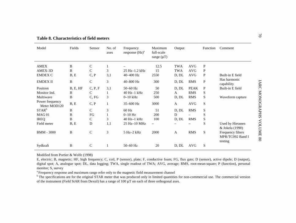
Survey meters are easy to use, portable and convenient for measuring fieldmagnitudes over wide areas or in selected locations. Three-axis survey meters arecapable of simple signal processing, such as computing the resultant field, storingmultiple measurements in their memory or averaging measurements. It is important tonote that the resultant field can be equal to, or up to 40% greater (for a circularlypolarized field) than, the maximum field measured by a single-axis meter (IEEE,1995a). Computer-based waveform capture measurement systems are designed toperform sophisticated signal processing and to record signals over periods rangingfrom a fraction of a second to several days. The instruments discussed here are thosemost commonly used for measuring fields in the environment or laboratory (Table 7).The measurement capabilities of selected instruments are summarized in Table 8. Lessfrequently used instruments designed for special purposes are described elsewhere(e.g. WHO, 1984, 1987). The operation of the electric and magnetic field metersrecommended for use is described in IEEE (1995a) and IEC (1998).


Resultant = )ZYX 222( ++

IARC M

ON

OG

RAPH

S VO

LUM

E 8068

Table 7. General characteristics of intruments

Meter type Primary uses Field parametersmeasured

Data-collectionfeatures

Cost Ease of use Data recording Portability

Spotmeasurements

AC/DC fieldmagnitude (x,y,z,resultant)

Full waveformcapture

Very high High-level technicalunderstanding required

Digitizedrecordingfeatures

Less portablethan typicalmeters

Mapping AC field magnitude ateach frequency ofinterest (x,y,z axes,resultant)

Computer-basedwaveformmeasure-mentsystems

Long-termmeasurements

AC field polarization

Waveform capture AC–DC orientationTransient capture Peak-to-peak

Highest quantifi-cation content in datacollection

The vast quantitiesof data collected are difficultto manage (approximately 50kbytes for an average spotmeasurement vs. 10 byteswith a three-axis AC-fieldrecording meter)

5-kg‘portable’systemcommerciallyavailable

Three-axisAC fieldrecordingroot-mean-squaremeter

Personal exposureSpotmeasurements

AC field magnitude(x,y,z axes, resultant)in a bandwidthdependent upon model

Medium–high

Almost no instructionrequired for accurate resultantmeasurements

Recordingfeatures

Small,portable

MappingLong-termmeasurements

Many have softwarefor mappingcapabilities if usedwith mapping wheel

Exploratorymeasurements

Some models canprovide harmoniccontent

More difficult to use forexploratory measurements(‘sniffing’) than single-axismeters because of delaybetween readouts

SOU

RCES, EXPO

SURE A

ND

EXPO

SURE A

SSESSMEN

T69

Table 7 (contd)

Meter type Primary uses Field parametersmeasured

Data-collectionfeatures

Cost Ease of use Data recording Portability

Three-axiscumulativeexposuremeter withdisplay

Personal exposureSpotmeasurementsExploratorymeasurementsLong-termmeasurements forcumulativeinformation

AC field magnitude(x,y,z axes, resultant)in a bandwidthdependent upon model

Most frequently usedfor personal exposuremeasurements

Medium Almost no instructionrequired for accurate resultantmeasurements

Recordsaccumulateddata, rather thanindividualsamples

Small,portable

Three-axisAC-fieldsurveymeter

Spotmeasurements

AC-field magnitude(x,y,z axes, resultant)in a bandwidthdependent upon model

Medium Almost no instructionrequired for accurate resultantmeasurement

No recordingfeature

Small,portable


Some models canprovide total harmoniccontent

Similar to three-axisrecording meters,with recordingcapabilities

More difficult to use forexploratory measurements(‘sniffing’) than single-axismeters because of delaybetween readouts

Single-axisAC-fieldsurveymeter


AC field magnitude inone direction, in abandwidth dependentupon model

Can be used todeterminepolarization

Low Continuous readout provideseasy source investigation

No recordingfeature

Small,portable

Spotmeasurements

Some models can beswitched from flat tolinear response toprovide rough data onpresence of harmonics

Easy determinationof direction of fieldCan be used with anaudio attachment.For exploratorymeasurements

Maximum field must be‘found’ by properly rotatingthe meter, or measuring inthree orthogonal directions tocalculate the resultant field

AC, alternating current; DC, direct currentFor further details and handling information, see IEC (1998).

IARC M

ON

OG

RAPH

S VO

LUM

E 8070

Table 8. Characteristics of field meters

Model Fields Sensor No. ofaxes

Frequencyresponse (Hz)a

Maximumfull-scalerange (μT)

Output Function Comment

AMEX B C 1 – 12.5 TWA AVG PAMEX-3D B C 3 25 Hz–1.2 kHz 15 TWA AVG PEMDEX C B, E C, P 3,1 40–400 Hz 2550 D, DL AVG P Built-in E field

EMDEX II B C 3 40–800 Hz 300 D, DL RMS P Has harmoniccapability

Positron B, E, HF C, P, F 3,1 50–60 Hz 50 D, DL PEAK P Built-in E fieldMonitor Ind. B C 1 40 Hz–1 kHz 250 A RMS SMultiwave B C, FG 3 0–10 kHz 500 D, DL RMS S Waveform capturePower frequency Meter MOD120 B, E C, P 1 35–600 Hz 3000 A AVG S

STARb B C 3 60 Hz 51 D, DL RMS SMAG 01 B FG 1 0–10 Hz 200 D – SIREQ B C 3 40 Hz–1 kHz 100 D, DL RMS SField meter B, E D 1,1 25 Hz–10 MHz – – – S Used by Hietanen

& Jokela (1990)BMM - 3000 B C 3 5 Hz–2 kHz 2000 A RMS S Frequency filters

MPR/TC092 Band Itesting

Sydkraft B C 1 50–60 Hz 20 D, DL AVG S

Modified from Portier & Wolfe (1998)E, electric; B, magnetic; HF, high frequency; C, coil, P (sensor), plate; F, conductive foam; FG, flux gate; D (sensor), active dipole; D (output),digital spot; A, analogue spot; DL, data logging; TWA, single readout of TWA; AVG, average; RMS, root-mean-square; P (function), personalmonitor; S, surveya Frequency response and maximum range refer only to the magnetic field measurement channelb The specifications are for the original STAR meter that was produced only in limited quantities for non-commercial use. The commercial versionof the instrument (Field StAR from Dexsil) has a range of 100 μT on each of three orthogonal axes.

(a) Electric fields(i) Survey meters

The meters commonly used in occupational and environmental surveys of electricfields are small both for convenience and to minimize their effect on the electric fieldbeing measured. To measure the unperturbed field, the meter is suspended at the endof a long non-conductive rod or tripod to minimize interference with the measurementby the investigator. In an oscillating electric field, the current measured between twoisolated conducting parts of the sensor is proportional to the field strength. Theaccuracy of the measurements obtained with these instruments is generally high,except under the following conditions:

• extremes of temperature and humidity;• insufficient distance of the probe from the investigator;• instability in meter position;• loss of non-conductive properties of the supporting rod.Electric fields can also be measured at fixed locations, e.g. under transmission

lines or in laboratory exposure chambers by measuring the current collected by a flatconducting plate placed at ground level. For sinusoidal fields, the electric flux densitycan be calculated from the area of the plate (A), the permittivity of a vacuum (ε0), thefrequency ( f ) and the measured current induced in the plate (Irms) in the expressionbelow:

IrmsE = ______

2π f ε0A

Electric field meters can be calibrated by placing the probe in a uniform field producedbetween two large conducting plates for which the field strength can be easilycalculated (IEEE, 1995a, b).

(ii) Personal exposure meters for measuring electric fieldsPersonal exposure meters are instruments for measuring the exposure of a person

to electric fields in various environments, e.g. work, home and travel (see below forpersonal exposure meters for measuring magnetic fields). However, wearing a meter onthe body perturbs the electric field being measured in unpredictable ways. Typically,where exposure to electric fields of large groups of subjects is being measured, a meteris placed in an armband, shirt pocket or belt pouch (Male et al., 1987; Bracken, 1993).Perturbation of the ambient field by the body precludes obtaining an absolute value ofthe field and, at best, the average value of such measurements reflects the relative levelof exposure.


(b) Magnetic fields(i) Survey meters

Magnetic fields can be measured with a survey meter, fixed location monitor or awearable field meter. The simplest meter measures the voltage induced in a coil ofwire. For a sinusoidally varying magnetic field, B, of frequency f, the voltage, V,induced in the coil is given by:

V = –2π f B0Acosωtwhere f is the frequency of the field and ω = 2πf, A is the area of the loop, and B0 isthe component of B perpendicular to the loop.

The voltage induced by a given field increases with the addition of turns of wire orof a ferromagnetic core. To prevent interference from electric fields, the magnetic fieldprobe must be shielded. If the meter is used for surveys or personal exposure measure-ments, frequencies lower than approximately 30 Hz must be filtered out to removevoltages induced in the probe by the motion of the meter in the earth’s magnetic field.

The presence of higher frequencies, such as harmonics, can affect magnetic fieldmeasurements depending on the frequency response of the magnetic field meter. Thefrequency response of three different meters is illustrated in Figure 5 (modified fromJohnson, 1998). These meters are calibrated so that a 60-Hz, 0.1-μT field reads as 0.1 μTon all three instruments. The narrow-band meter focuses on the 60-Hz magnetic fieldand greatly attenuates the sensitivity of the meter to higher and lower frequencies. Thebroadband meter provides an accurate measurement of the magnetic field across a widerfrequency range because it has a flat frequency response between 40 Hz and 1000 Hz.The broadband meter with a linear response provides very different measurements in thisrange as the magnetic field reading is weighted by its frequency (Johnson, 1998).


Figure 5. Frequency response of linear broadband, flat broadband and narrow-band magnetic-field meters to a reference field of 0.1 μμT

Modified from Johnson (1998)

Fluxgate magnetometers have adequate sensitivity for measuring magnetostaticfields in the range 0.1 μT–0.01 T. Above 100 μT, both AC and DC magnetic fields canbe measured using a Hall effect sensor (IEEE, 1995b). The sensor is designed tomeasure the voltage across a thin strip of semiconducting material carrying a controlcurrent. The voltage change is directly related to the magnetic flux density of AC andDC magnetic fields (Agnew, 1992).

Early survey meters made average field readings and then extrapolated them toroot-mean-square values by applying a calibration factor. These meters give erroneousreadings when in the presence of harmonics and complex waveforms.

(ii) Personal exposure meters for measuring magnetic fieldsWearable meters for measuring magnetic fields have facilitated assessments of the

personal exposure of individuals as they go about daily activities at home, school andwork. A few instruments can also record electric-field measurements. The availablepersonal exposure meters can integrate field readings in single or multiple data registersover the course of a measurement period. For a single-channel device, the result is asingle value representing the integrated exposure over time in μT·h or (kV/m) h. Somemeters classify and accumulate exposures into defined intensity ‘bins’. Other personalexposure meters collect samples at fixed intervals and store the measurements incomputer memory for subsequent downloading and analysis (see Table 9).

One of the most popular instruments used in occupational surveys and epidemio-logical studies is the electric and magnetic field digital exposure system (EMDEX). TheEMDEX II data logger records the analogue output from three orthogonal coils or thecomputed resultant magnetic field. It can also record the electric field detected by aseparate sensor. Different versions of the meter are used for environmental field ranges(0.01 μT–0.3 mT) and near high intensity sources (0.4 μT–12 mT) (data from the manu-facturer, 2001).

Smaller, lighter versions of the EMDEX are available to collect time series recordsover longer time periods (EMDEX Lite) or to provide statistical descriptors ⎯ mean,standard deviation, minimum, maximum and accumulated time above specifiedthresholds ⎯ of accumulated measurements (EMDEX Mate). The AMEX (averagemagnetic exposure)-3D measures only the average magnetic field over time of use.IEC (1998) has provided detailed recommendations for the use of instruments inmeasuring personal exposure to magnetic fields.

(iii) Frequency responseThe bandwidth of magnetic field meters is generally between 40 Hz and 1000 Hz.

Further differentiation of field frequency within this range is not possible unlessfiltered to a narrow frequency band of 50 or 60 Hz. However, a data logger, theSPECLITE®, was employed in one study to record the magnetic field in 30 frequencybins within this range at 1-min intervals (Philips et al., 1995).



Table 9. Commercially available instruments for measuring ELF magnetic fieldsa

Company, location Meter, field type Frequency range

AlphaLab Inc.Salt Lake City, Utah, USA

Bartington Instruments LtdOxford, England

Combinova ABBromma, Sweden

TriField Meter (3-axis E, M & RF) 50 Hz–3 GHz

MAG-01 (1-axis M) DC–a few kHzMAG-03 (3-axis M) 0 Hz–3000 Hz

MFM 10 (3-axis M recording) 20 Hz–2000 HzMFM 1020 (3-axis E, M recording) 5 Hz–400 kHzFD 1 (E, 3-axis M survey) 20 Hz–2000 HzFD 3 (3-axis M recording) 20 Hz–2000 Hz

Dexsil Corp.Hamden, Connecticut, USA

Electric ResearchPittsburgh, Pennsylvania, USA

Field Star 1000 (3-axis M recording) not specifiedField Star 4000 (3-axis M recording) not specifiedMagnum 310 (3-axis M survey) 40 Hz–310 Hz

MultiWave® System II(E, M 3-axis, waveform) 0–3000 Hz

Enertech ConsultantsCampbell, California, USA

EMDEX SNAP (3-axis M survey) 40 Hz–1000 HzEMDEX PAL (3-axis M limited recording) 40 Hz–1000 HzEMDEX MATE (3-axis M limited recording) 40 Hz–1000 HzEMDEX LITE (3-axis M recording) 10 Hz–1000 HzEMDEX II (3-axis E & M recording) 40 Hz–800 HzEMDEX WaveCorder (3-axis M waveform) 10 Hz–3000 HzEMDEX Transient Counter (3-axis M) 2000 Hz–220 000 Hz

EnviroMentor ABMölndal, Sweden

Holaday Industries, Inc.Eden Prairie, Minnesota, USA

Field Finder Lite (1-axis M & E) 15 Hz–1500 HzField Finder (3-axis M & 1-axis E) 30 Hz–2000 HzML-1 (3-axis M, 3-dimensional presentation) 30 Hz–2000 HzBMM-3000 (3-axis M, analysis program) 5 Hz–2000 Hz

HI-3624 (M) 30 Hz–2000 HzHI-3624A (M) 5 Hz–2000 HzHI-3604 (E, M) 30 Hz–2000 HzHI-3627 (3-axis M, recorder output) 5 Hz–2000 Hz

Magnetic Sciences InternationalActon, Massachusetts, USA

MSI-95 (1-axis M) 25 Hz–3000 HzMSI-90 (1-axis M) 18 Hz–3300 HzMSI-25 (1-axis M) 40 Hz–280 Hz

Physical Systems InternationalHolmes Beach, Florida, USA

Sypris Test and MeasurementOrlando, Florida, USA

FieldMeter (1-axis E, M) 16 Hz–5000 HzFieldAnalyzer (1-axis E, 3-axis M, waveform) 1 Hz–500 Hz

4070 (1-axis M) 40 Hz–200 Hz4080 (3-axis M) 40 Hz–600 Hz4090 (3-axis M) 50 Hz–300 Hz7030 (3-axis M) 10 Hz–50 000 Hz

Tech International Corp.Hallandale, Florida, USA

CellSensor (1-axis M & RF) ∼50 Hz–∼835 MHz

Specialized wave-capture instruments, such as the portable MultiWave system, canmeasure static and time-varying magnetic fields at frequencies of up to 3 kHz (Bowman& Methner, 2000). The EMDEX WaveCorder can also measure and record the wave-form of magnetic fields for display and downloading.

In addition to measuring power-frequency fields, the Positron meter was designedto detect pulsed electric and magnetic fields or high-frequency transients associatedwith switching operations in the utility industry (Héroux, 1991). Only after its use intwo epidemiology studies was it discovered that the readings of the commercial sensorswere erratic and susceptible to interference from radiofrequency fields outside thebandwidth specification of the sensor. The interference by radio signals from hand-heldwalkie-talkies and other communication devices was recorded (Maruvada et al., 2000).

The EMDEX Transient Counter, which has recently been developed, continuouslymeasures changes in magnetic fields at frequencies between 2000 Hz and 220 000 Hzand reports the number of times that the change in amplitude exceeds thresholds of5 nT and 50 nT (data from the manufacturer, 2001).

A list of some currently available instruments for measuring magnetic fields isgiven in Table 9.

1.2.2 Computation methods

For many sources, measurements are the most convenient way to characterizeexposure to ELF electric and magnetic fields. However, unperturbed fields fromsources such as power lines can also be easily characterized by calculations. Calculatedelectric field intensity and direction may differ from those that are measured becauseof the presence of conductive objects close to the source and/or near the location ofinterest.

The fields from power lines can be calculated accurately if the geometry of theconductors, the voltages and currents (amplitude and phase angle) in the conductors and


Table 9 (contd)

Company, location Meter, field type Frequency range

Technology Alternatives Corp.Miami, Florida, USA

Walker LDJ Scientific, Inc.Worcester, Massachusetts, USA

ELF Digital Meter (M) 20 Hz–400 HzELF/VLF Combination Meter (M) 20 Hz–2000 Hz ELF; 10.000 Hz–200 000 Hz VLF

ELF 45D (1-axis M) 30 Hz–300 HzELF 60D (1-axis M) 40 Hz–400 HzELF 90D (3-axis M) 40 Hz–400 HzBBM-3D (3-axis M, ELF & VLF) 12 Hz–50 000 Hz

Source: Microwave News (2002) and industry sourcesE, electric; M, magnetic (50 or 60 Hz); RF, radiofrequency; ELF, extremely low frequency; VLF, very lowfrequencya Some instruments are suitable for measuring both magnetic and electric fields.

return paths are known. The currents flowing in the conductors of power lines are typi-cally logged at substations and historical line-loading data may be available. However,in some cases, currents do not all return to utility facilities and may flow into the earthor into any conductor which is at earth potential, such as a neutral wire, telephone wire,shield wire or buried piping. Because the magnitude and location of the currents on thesepaths are not known, it is difficult or impossible to include them in computations.

The simplest calculations assume that the conductors are straight, parallel andlocated above, and parallel to, an infinite flat ground plane. Balanced currents are alsotypically assumed. Calculations of magnetic fields that do not include the contributionof small induced currents in the earth are accurate near power lines, but may not be soat distances of some hundreds of metres (Maddock, 1992). Very accurate calculations ofthe maximum, resultant and vector components of electric and magnetic fields arepossible if the actual operating conditions at the time of interest are known, including thecurrent flow and the height of conductors, which vary with ambient temperature and lineloading.

A number of computer programs have been designed for the calculation of fieldsfrom power lines and substations. These incorporate useful features such as thecalculation of fields from non-parallel conductors. While the computation of simplefields by such programs may be quite adequate for their intended purpose, it may bedifficult for other investigators to verify the methods used to calculate exposures.Epidemiological studies that estimated the historical exposures of subjects to magneticfields from power lines by calculations did not usually report using documentedcomputer programs or publish the details of the computation algorithms, e.g. Olsenet al. (1993), Verkasalo et al. (1993, 1996), Feychting and Ahlbom (1994), Tynes andHaldorsen (1997) and UK Childhood Cancer Study Investigators (2000a). However, forexposure assessment in these studies, it is likely that the uncertainty in the historicalloading on the power lines would contribute much more to the overall uncertainty inthe calculated field than all of the other parameters combined (Jaffa et al., 2000).

Calculations are also useful for the calibration of electric and magnetic fieldmeters (IEEE, 1995b) and in the design of animal and in-vitro exposure systems, e.g.Bassen et al. (1992), Kirschvink (1992), Mullins et al. (1993).

1.3 Exposure assessment

1.3.1 External dosimetry

(a) Definition and metricsExternal dosimetry deals with characterization of static and ELF electric and

magnetic fields that define exposure in epidemiological and experimental studies. Forstatic fields, the field strength (or flux density) and direction unambiguously describeexposure conditions. As with other agents, the timing and duration of exposure areimportant parameters, but the situation is more complex in the case of ELF fields. The


difficulty arises, not from the lack of ability to specify complete and unique charac-teristics for any given field, but rather from the large number of parameters requiringevaluation, and, more importantly, the inability to identify the critical parameters forbiological interactions.

Several exposure characteristics, also called metrics, that may be of biological signi-ficance have been identified (Morgan & Nair, 1992; Valberg, 1995). These include:

• intensity (strength) or the corresponding flux density, root mean square, averageor peak value of the exposure field; or a function of the field strength such asfield-squared;

• duration of exposure at a given intensity;• time (e.g. daytime versus night-time);• single versus repeated exposure;• frequency spectrum of the field; single frequency, harmonic content, inter-

mittency, transients; • spatial field characteristics: orientation, polarization, spatial homogeneity

(gradients);• single field exposure, e.g. ELF magnetic versus combined electric and

magnetic field components, and possibly their mutual orientation; • simultaneous exposure to a static (including geomagnetic field) and ELF field,

with a consideration of their mutual orientation;• exposure to ELF fields in conjunction with other agents, e.g. chemicals.

The overall exposure of a biological system to ELF fields can be a function of theparameters described above (Valberg, 1995).

(b) Laboratory exposure systemsLaboratory exposure systems have the advantage that they can be designed to

expose the subjects to fields of specific interest and the fields created are measurableand controllable. Laboratory exposure systems for studying the biological effects ofelectric and magnetic fields are readily classified as in vivo or in vitro. Most studies ofexposure in vivo have been in animals; few have involved humans. In-vitro studies ofexposure are conducted on isolated tissues or cultured cells of human or animal origin.

One reason for studying the effects of very strong fields is the expectation thatinternal dose is capable of being biologically scaled. For this reason, many laboratoryexperiments have been performed at field strengths much higher than those normallymeasured in residential and occupational settings. This approach is usually used on theassumption that the amplitude of biological effects increases with field strength up to themaxima set in exposure guidelines, and the physical limitations of the exposure system.

(i) In-vivo exposure systemsMany in-vivo studies have used magnetostatic fields (Tenforde, 1992; see also

section 4). Both iron-core electromagnets and permanent magnets are routinely used insuch studies. Although it is theoretically possible to obtain even larger DC magnetic


fields from iron-core devices (up to approximately 2 T), there is a limitation on the sizeof the active volume between the pole faces where the field is sufficiently uniform.Experimental studies of fields greater than 1.5 T are difficult because limited space isavailable for exposing biological systems to reasonably uniform magnetic fields.

The most commonly used apparatus for studying exposure to electric fieldsconsists of parallel plates between which an alternating voltage (50 or 60 Hz, or otherfrequencies) is applied. Typically, the bottom plate is grounded. When appropriatedimensions of the plates are selected (i.e. a large area in comparison to the distancebetween the plates), a uniform field of reasonably large volume can be producedbetween the plates. The distribution of the electric-field strength within this volumecan be calculated. The field becomes less uniform close to the plate edges.

A uniform field in an animal-exposure system can be significantly perturbed bytwo factors. An unavoidable but controllable perturbation is due to the presence of testanimals and their cages. Much information is available on correct spacing of animalsto ensure similar exposure for all test animals and to limit the mutual shielding of theanimals (Kaune, 1981a; Creim et al., 1984). Animal cages, drinking bottles, food andbedding cause additional perturbations of the electric field (Kaune, 1981a). One of themost important causes of artefactual results in some studies is induction of currents inthe nozzle of the drinking-water container. If the induced currents are sufficientlylarge, animals experience electric microshocks while drinking. Corrective measureshave been developed to alleviate this problem (Free et al., 1981). Perturbation of theexposure field by nearby metallic objects is easy to prevent. The faulty design,construction and use of the electric-field-exposure facility can result in unreliableexposure over and above the limitations that normally apply to animal bioassays.

A magnetic field in an animal-exposure experiment is produced by current flowingthrough an arrangement of coils. The apparatus can vary from a simple set of twoHelmholtz coils (preferably square or rectangular to fit with the geometry of cages), toan arrangement of four coils (Merritt et al., 1983), to more complicated coil systems(Stuchly et al., 1991; Kirschvink, 1992; Wilson et al., 1994; Caputa & Stuchly, 1996).The main objectives in designing apparatus for exposure to magnetic fields are (1) toensure the maximal uniformity of the field within as much as possible of the volumeencompassed by the coils, and (2) to minimize the stray fields outside the coils, so thatsham-exposure apparatus can be placed in the same room. Square coils with fourwindings arranged according to the formulae of Merritt et al. (1983) best satisfy thefield-uniformity requirement. Limiting the stray fields is a challenge, as shieldingmagnetic fields is much more complex than shielding electric fields. Non-magneticmetal shields only slightly reduce the field strength. Only properly designed multilayer-shielding enclosures made of high-permeability materials are effective. An alternativesolution relies on partial field cancellation. Two systems of coils placed side by side orone above the other form a quadrupole system that effectively decreases the magneticfield outside the exposure system (Wilson et al., 1994). An even greater reduction isobtained with a doubly compensating arrangement of coils. Four coils (each consisting


of four windings) are arranged side by side and up and down; coils placed diagonallyare in the same direction as the field, and the neighbouring coils are in the oppositedirection (Caputa & Stuchly, 1996).

Likely artefacts associated with magnetic-field-exposure systems include heating,vibrations and audible or high-frequency (non-audible to humans) noise. These factorscan be minimized (although not entirely eliminated) with careful design andconstruction, which can be costly. The most economical and reliable way of over-coming these problems is through essentially identical design and construction of thefield- and sham-exposure systems except for the current direction in bifilarly woundcoils (Kirschvink, 1992; Caputa & Stuchly, 1996). This solution provides for the sameheating of both the control and exposed systems. Vibration and noise are usually notexactly the same but are similar. To limit the vibration and noise, the coil windingsshould be restricted mechanically in their motion.

Another important feature of a properly designed magnetic-field system isshielding against the electric field produced by the coils. Depending on the coil shape,the number of turns in the coil and the diameter of the wire, a large voltage drop canoccur between the ends of the coils. Shielding of the coils can eliminate interferencefrom the electric field.

(ii) In-vitro exposure systemsCell and tissue cultures can be exposed to the electric field produced between

parallel plates in the same way that animals are exposed. In practice, this procedure ishardly ever used, because the electric fields in the in-vitro preparation produced this wayare very weak, even for strong applied fields. For instance, an externally applied field of10 kV/m at 60 Hz results in only a fraction of a volt per metre in the culture (Tobey et al.,1981; Lymangrover et al., 1983). Furthermore, the field strength is usually not uniformthroughout the culture, unless the culture is thin and is placed perpendicular or parallelto the field. A practical solution involves the placement of appropriate electrodes in thecultures. Agar or other media bridges can be used to eliminate the problem of electrodecontamination (McLeod et al., 1987). A comprehensive review of in-vitro exposuresystems has recently been published (Misakian et al., 1993).

The shape and size of the electrodes determine the uniformity of the electric fieldand associated spatial variations of the current density. Either accurate modelling ormeasurements, or preferably both, should be performed to confirm that the desiredexposure conditions are achieved. Additional potential problems associated with thistype of exposure system are the heating of the medium and accompanying inducedmagnetic fields. Both of these factors can be evaluated (Misakian et al., 1993).

Coils similar to those used for animal studies can be used for in-vitro experiments(Misakian et al., 1993). The greatest uniformity is achieved along the axis within thevolume enclosed in the solenoid. One great advantage of solenoids over Helmholtzcoils is that the uniform region within the solenoid extends from the axis across thewhole of the cross-sectional diameter.


In in-vitro studies, special attention should be paid to ambient levels of 50 or 60 Hzand to other magnetic fields. Magnetic flux densities from incubators unmodified forbioeffect studies may have background gradients of magnetic fields ranging from a fewtenths of a microtesla to approximately 100 μT. Similarly, some other laboratoryequipment with an electric motor might expose biological cells to high, but unaccountedfor, magnetic flux densities. Specially designed in-vitro systems can avoid theseproblems. Exposure to magnetic fields that is unaccounted for or is at an incorrect level,as well as the critical influence of temperature and carbon dioxide concentration on somecell preparations, can lead to unreliable findings in laboratory experiments (Misakianet al., 1993).

In some in-vitro studies, simultaneous exposure to alternating and static magneticfields is used in a procedure intended to test the hypothesis of possible ‘resonant’effects. Almost all the requirements for controlled exposure to the alternating fieldapply to the static field. Some precautions are not required in static field systems. Forexample, static systems have no vibrations (with the possible exception of on and offswitching) so prevention of vibrations is unnecessary. In experiments involving staticmagnetic fields, the earth’s magnetic field should be measured and controlled locally.

1.3.2 Internal dosimetry modelling

(a) Definition for internal dosimetry At ELF, electric fields and magnetic fields can be considered to be uncoupled

(Olsen, 1994). Therefore, internal dosimetry is also evaluated separately. For simulta-neous exposure to both fields, internal measures can be obtained by superposition.Exposure to either electric or magnetic fields results in the induction of electric fieldsand associated current densities in tissue. The magnitudes and spatial patterns of thesefields depend on the type of field (electric or magnetic), its characteristics (frequency,magnitude, orientation), and the size, shape and electrical properties of the exposed body(human, animal). Exposure to electric fields also results in an electric charge on the bodysurface.

The primary dosimetric measure is the induced electric field in tissue. The mostfrequently reported dosimetric measures are the average, root-mean-square andmaximum induced electric field and current density values (Stuchly & Dawson, 2000).Additional measures include the 50th, 95th and 99th percentiles which indicate valuesnot exceeded in a given volume of tissue, e.g. the 99th percentile indicates thedosimetric measure exceeded in 1% of a given tissue volume (Kavet et al., 2001). Theelectric field in tissue is typically expressed in μV/m or mV/m and the current densityin μA/m2 or mA/m2. Some safety guidelines (International Commission on Non-Ionizing Radiation Protection (ICNIRP), 1998) specify exposure limits measured asthe current density averaged over 1 cm2 of tissue perpendicular to the direction of thecurrent.


The internal (induced) electric field E and conduction current density J are relatedthrough Ohm’s law:

J = σEwhere the bold symbols denote vectors and σ is the bulk tissue conductivity whichmay depend on the orientation of the field in anisotropic tissues (e.g. muscle).

(b) Electric-field dosimetryEarly dosimetry models represented the human (or animal) body in a simplified

way, as reviewed elsewhere (Stuchly & Dawson, 2000). During the past 10 years,several laboratories have developed sophisticated heterogeneous models of the humanbody (Gandhi & Chen, 1992; Zubal et al., 1994; Gandhi, 1995; Dawson et al., 1997;Dimbylow, 1997). These models partition the body into volumes of different conducti-vity. Typically, over 30 distinct organs and tissues are identified and represented bycubic cells (voxels) with 1–10-mm sides. Voxels are assigned a conductivity valuebased on the measured values reported by Gabriel et al. (1996). A model of the humanbody constructed from several geometrical bodies of revolution has also been used(Baraton et al., 1993; Hutzler et al., 1994).

Various methods have been used to compute induced electric fields in these high-resolution models. Because of the low frequency involved, exposures to electric andmagnetic fields are considered separately and the induced vector fields are added, ifneeded. Exposure to electric fields is generally more difficult to compute than exposureto magnetic fields, since the human body significantly perturbs the electric field.Suitable numerical methods are limited by the highly heterogeneous electricalproperties of the human body and the complex external and organ shapes. The methodsthat have been successfully used so far for high-resolution dosimetry are: the finitedifference method in frequency domain and time domain, and the finite elementmethod. The advantages and limitations of each method have been reviewed by Stuchlyand Dawson (2000). Some of the methods and computer codes have been extensivelyverified by comparison with analytical solutions (Dawson & Stuchly, 1997).

Several numerical evaluations of the electric field and the current density induced invarious organs and tissues have been performed (Dawson et al., 1998; Furse & Gandhi,1998; Dimbylow, 2000; Hirata et al., 2001). Average organ (tissue) and maximum voxelvalues of the electric field and current density are typically reported. In the recent studies(Dimbylow, 2000; Hirata et al., 2001), the maximum current density was averaged over1 cm2 for excitable tissues. The latter computation is clearly aimed at testing compliancewith the International Commission on Non-Ionizing Radiation Protection (ICNIRP)guideline (1998) and the commentary published thereafter (Matthes, 1998).

The induced electric fields computed in various laboratories are in reasonableagreement (Stuchly & Gandhi, 2000). As expected, smaller differences are observedbetween calculated electric fields than between calculated values for current density.


The observed differences can be explained by differences between the body modelsand the conductivity values allocated to different tissues.

The differences observed in the results of high-resolution models depend in partupon the conductivity values assumed (Dawson et al., 1998). In general, the lower theinduced electric fields (the higher the current density) the higher the conductivity oftissue. The exceptions are those parts of the body associated with concave curvature,e.g. the tissue surrounding the armpits, where the electric field is enhanced. For thewhole body, the computed average values do not differ by more than 2% (Stuchly &Dawson, 2000).

The resolution of the model influences the accuracy with which the induced fieldsare evaluated in various organs. Organs that are small in any dimension are poorlyrepresented by large voxels. The maximum induced electric field is higher for the finerresolution. The differences are typically of the order of 50–190% for voxels of 3.6-mmsides compared to 7.2-mm voxels (Stuchly & Dawson, 2000).

The highest induced fields are found in a body that is in contact with perfectground through both feet. The average values for the organs or tissues of a ‘grounded’body are about two or three times those for a body in free space (Dawson et al., 1998),and intermediate values are obtained for various degrees of separation from theground. This dependence on the contact with or separation from a perfect ground is inagreement with earlier experimental data (Deno & Zaffanella, 1982).

The main features of dosimetry for exposure of a person standing in an ELFelectric field can be summarized as follows:

• The magnitudes of the electric fields in tissue are typically 10–5–10–8 lowerthan the magnitude of the external field.

• For exposure to external fields from power lines, the predominant direction ofthe induced fields is also vertical.

• The largest fields in a human body are induced by a vertical electric field whenthe feet are in contact with a perfectly conducting ground plane.

• The weakest fields are induced in a body when it is in free space, i.e. infinitelyfar from the ground plane.

• The short-circuit current for a body in contact with perfect ground is determinedby the size and shape of the body (including posture), rather than its tissueconductivity.

Table 10 summarizes the computed internal electric fields for a model of an adultbody in a vertical field of 1 kV/m at 60 Hz (Kavet et al., 2001), where the body (1.77 min height and 76 kg in weight) makes contact with a perfectly conducting ground withboth feet. Table 11 summarizes computed internal electric fields for a model of a five-year-old child (1.10 m in height and 18.7 kg in weight) (Hirata et al., 2001). Selectedconductivity values are given in Table 2 of the General Introduction. Dawson et al.(2001) demonstrated that the voxel maximum values are significantly overestimated,and the 99th percentiles are therefore more representative.


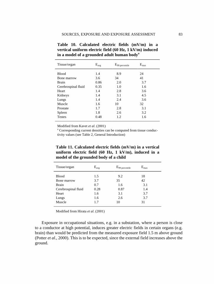
Exposure in occupational situations, e.g. in a substation, where a person is closeto a conductor at high potential, induces greater electric fields in certain organs (e.g.brain) than would be predicted from the measured exposure field 1.5 m above ground(Potter et al., 2000). This is to be expected, since the external field increases above theground.


Table 10. Calculated electric fields (mV/m) in avertical uniform electric field (60 Hz, 1 kV/m) inducedin a model of a grounded adult human bodya

Tissue/organ Eavg E99 percentile Emax

Blood 1.4 8.9 24Bone marrow 3.6 34 41Brain 0.86 2.0 3.7Cerebrospinal fluid 0.35 1.0 1.6Heart 1.4 2.8 3.6Kidneys 1.4 3.1 4.5Lungs 1.4 2.4 3.6Muscle 1.6 10 32Prostate 1.7 2.8 3.1Spleen 1.8 2.6 3.2Testes 0.48 1.2 1.6

Modified from Kavet et al. (2001)a Corresponding current densities can be computed from tissue conduc-tivity values (see Table 2, General Introduction)

Table 11. Calculated electric fields (mV/m) in a verticaluniform electric field (60 Hz, 1 kV/m), induced in amodel of the grounded body of a child


Blood 1.5 9.2 18Bone marrow 3.7 35 42Brain 0.7 1.6 3.1Cerebrospinal fluid 0.28 0.87 1.4Heart 1.6 3.1 3.7Lungs 1.6 2.6 3.7Muscle 1.7 10 31

Modified from Hirata et al. (2001)

(c) Magnetic-field dosimetryEarly dosimetry models represented the body as a circular loop corresponding to

a given body contour to determine the induced electric field or current density basedon Faraday’s law:

| J | = πfσr | B |where f is the frequency, r is the loop radius and B is the magnetic flux density vectorperpendicular to the current loop. Similarly, ellipsoidal loops have been used to fit thebody shape better.

More realistic models of the human body have been analysed by the numericalimpedance method (Gandhi & De Ford, 1988; Gandhi & Chen, 1992; Gandhi et al.,2001) and the scalar potential finite difference technique (Dawson & Stuchly, 1998;Dimbylow, 1998). The dosimetry data available for magnetic fields are more extensivethan those for electric fields. The effects of tissue properties in general (and specificallymuscle anisotropy), field orientation with respect to the body and, to a certain extent,body anatomy have been investigated (Dawson et al., 1997; Dawson & Stuchly, 1998;Dimbylow, 1998). In the past, the largest loop of current fitted within a body part, e.g.head or heart, was often used to calculate the maximum current density in that bodypart. This is now known to underestimate the maximum induced field and the currentdensities (Stuchly & Dawson, 2000)

The main features of dosimetry for exposure to uniform ELF magnetic fields canbe summarized as follows:

• The induced electric fields depend on the orientation of the magnetic field withrespect to the body.

• For most organs and tissues, the magnetic field orientation perpendicular to thetorso (front-to-back) gives maximum induced quantities.

• For the brain, cerebrospinal fluid, blood, heart, bladder, eyes and spinal cord,the strongest induced electric fields are produced by a magnetic field directedtowards the side of the body.

• Magnetic fields oriented along the vertical body axis induce the weakestelectric fields.

• Stronger electric fields are induced in bodies of larger size.Table 12 lists the electric fields induced in certain organs and tissues by a 60-Hz,

1-μT magnetic field oriented front-to-back (Dawson et al., 1997; Dawson & Stuchly,1998; Kavet et al., 2001).

The exposure of humans to relatively high magnetic flux densities occurs mostoften in occupational settings. Numerical modelling has been applied mostly to workersexposed to high-voltage power lines (Baraton & Hutzler, 1995, Stuchly & Zhao, 1996;Dawson et al., 1999a,b,c). In these cases, current-carrying conductors can berepresented as infinite straight-line sources. However, some of the exposure occurs inmore complex scenarios, two of which have been analysed, and a more realisticrepresentation of the source conductors based on finite line segments has been used


(Stuchly & Dawson, 2000). Table 13 lists calculated electric fields for the two repre-sentative exposure scenarios illustrated in Figure 6 (Stuchly & Dawson, 2000).


Table 12. Calculated electric fields (μμV/m) in a uni-form magnetic field (60 Hz, 1 μμT) oriented front-to-back induced in a model of an adult human


Blood 6.9 23 83Bone marrow 16 93 154Brain 11 31 74Cerebrospinal fluid 5.2 17 25Heart 14 38 49Kidneys 25 53 71Lungs 21 49 86Muscle 15 51 147Prostate 17 36 52Spleen 41 72 92Testes 15 41 73

Modified from Kavet et al. (2001)

Table 13. Calculated electric fields (mV/m) induced in a modelof an adult human for the occupational exposure scenariosshown in Figure 6 (total current in conductors, 1000 A)

Scenario A Scenario BTissue/organ

Emax Erms Emax Erms

Blood 20 3.7 15 2.4Bone 90 11 58 7.2Brain 22 4.6 28 5.9Cerebrospinal fluid 9.2 2.3 14 3.7Heart 27 11 9.0 3.2Kidneys 22 7.9 2.8 0.9Lungs 31 10 9.9 2.9Muscle 59 6.9 33 5.5Prostate 5.5 1.9 2.6 1.2Testes 18 5.5 2.7 1.2

Modified from Stuchly & Dawson (2000)

(d ) Contact-current dosimetryContact currents produce electric fields in tissue similar to those induced by external

electric and magnetic fields. Contact currents are encountered in a dwelling or work-place when a person touches conductive surfaces at different potentials and completes apath for current flow through the body. The current pathway is usually from hand-to-hand and/or from a hand to one or both feet. Sources of contact current may include anappliance chassis or household fixture that, because of typical residential wiringpractices, carries a small potential above a ground. Other sources of contact current areconductive objects situated in an electric field, such as a vehicle parked under a powerline. The importance of contact currents has been suggested by Kavet et al. (2000).Recently, electric fields have been computed in a model of a child with electrodes onhands and feet simulating contact current (Dawson et al., 2001). The most commonsource of exposure to contact current is touching an ungrounded object while both feetare grounded. The electric fields calculated to be induced in the bone marrow of the handand arm of a child for a 1-μA contact current are shown in Table 14. Electric fields above1 mV/m can be produced in the bone marrow of a child from a low contact current of1 μA. In residential settings such a current could result from an open-circuit voltage ofonly 100 mV, which is not uncommon. A total resistance of 5–10 kΩ is representative(Kavet et al., 2000). Provided that there is good contact to the ground, only 5–10 mV isneeded to produce a current of 1–2 μA. Contact current with vehicles in an electric field


Figure 6. Body positions in two occupational exposure scenarios

From Stuchly & Dawson (2000)The current in each conductor is 250 A for a total of 1000 A in four conductors.

(e.g. under high-voltage power lines) typically ranges from 0.1 mA per 1 kV/m for a carto 0.6 mA per 1 kV/m for a large truck (Deno & Zaffanella, 1982).

(e) Biophysical relevance of induced fieldsThe lowest electric field in tissue to be associated with well-documented biological

effects (not necessarily harmful) has been estimated as 1 mV/m (Portier & Wolfe,1998). It is interesting to compare the different exposure conditions that produce aninternal field of this magnitude. Table 15 shows the average exposure to electric andmagnetic fields required to induce a field of 1 mV/m in selected tissues (Stuchly &Dawson, 2000). Although the mechanisms for biological effects of fields at 1 mV/m areunclear, it is, nevertheless, interesting to compare the electric fields induced in humansby exposure to residential magnetic fields, electric fields and contact currents. Table 16shows that the electric field induced in a model of a child’s bone marrow (i.e. the tissueinvolved in leukaemia) is 10 times greater for the exposure to a contact current than forexposure to either the maximum electric or magnetic field encountered in a dwelling(Kavet et al., 2000).

( f ) Microscopic dosimetryMacroscopic dosimetry that describes induced electric fields in various organs and

tissues can be extended to more spatially refined models of subcellular structures topredict and understand biophysical interactions. The simplest cellular model for consi-dering linear systems requires evaluation of induced fields in various parts of a cell.Such models, for instance, have been developed to understand neural stimulation(Plonsey & Barr, 1988; Basser & Roth, 1991; Reilly, 1992; Malmivuo & Plonsey,1995). Computations are available as a function of the applied electric field and itsfrequency. Because cell membranes have high resistivity and capacitance (nearlyconstant for all mammalian cells and equal to 0.5–1 μF/cm2) (Reilly, 1992), at suffi-ciently low frequencies, high fields are produced at the two poles of the membrane. Thefield is nearly zero inside the cell, as long as the frequency of the applied field is belowthe membrane relaxation frequency (~ 1 MHz) (Foster & Schwan, 1995). The total


Table 14. Calculated electric field (mV/m)induced by a contact current of 60 Hz, 1 μμA,in voxels of bone marrow of a child

Body part Eavg E99 percentile

Lower arm 5.1 14.9Upper arm 0.9 1.4Whole body 0.4 3.3

Modified from Dawson et al. (2001)

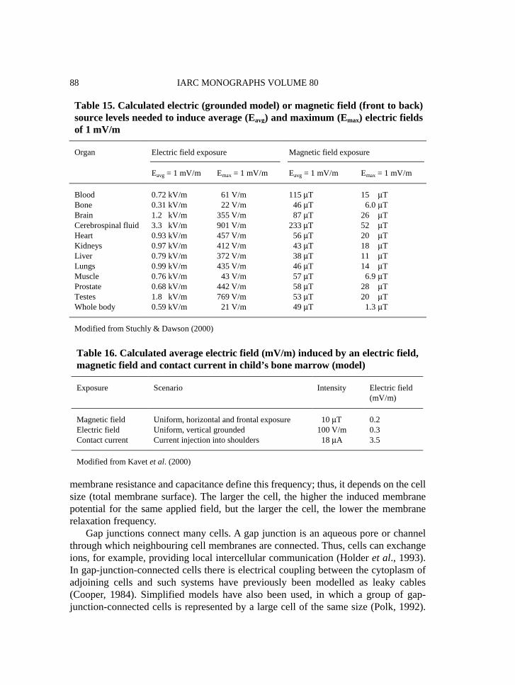
membrane resistance and capacitance define this frequency; thus, it depends on the cellsize (total membrane surface). The larger the cell, the higher the induced membranepotential for the same applied field, but the larger the cell, the lower the membranerelaxation frequency.

Gap junctions connect many cells. A gap junction is an aqueous pore or channelthrough which neighbouring cell membranes are connected. Thus, cells can exchangeions, for example, providing local intercellular communication (Holder et al., 1993).In gap-junction-connected cells there is electrical coupling between the cytoplasm ofadjoining cells and such systems have previously been modelled as leaky cables(Cooper, 1984). Simplified models have also been used, in which a group of gap-junction-connected cells is represented by a large cell of the same size (Polk, 1992).


Table 15. Calculated electric (grounded model) or magnetic field (front to back)source levels needed to induce average (Eavg) and maximum (Emax) electric fieldsof 1 mV/m

Electric field exposure Magnetic field exposureOrgan

Eavg = 1 mV/m Emax = 1 mV/m Eavg = 1 mV/m Emax = 1 mV/m

Blood 0.72 kV/m 61 V/m 115 μT 15 μTBone 0.31 kV/m 22 V/m 46 μT 6.0 μTBrain 1.2 kV/m 355 V/m 87 μT 26 μTCerebrospinal fluid 3.3 kV/m 901 V/m 233 μT 52 μTHeart 0.93 kV/m 457 V/m 56 μT 20 μTKidneys 0.97 kV/m 412 V/m 43 μT 18 μTLiver 0.79 kV/m 372 V/m 38 μT 11 μTLungs 0.99 kV/m 435 V/m 46 μT 14 μTMuscle 0.76 kV/m 43 V/m 57 μT 6.9 μTProstate 0.68 kV/m 442 V/m 58 μT 28 μTTestes 1.8 kV/m 769 V/m 53 μT 20 μTWhole body 0.59 kV/m 21 V/m 49 μT 1.3 μT

Modified from Stuchly & Dawson (2000)

Table 16. Calculated average electric field (mV/m) induced by an electric field,magnetic field and contact current in child’s bone marrow (model)

Exposure Scenario Intensity Electric field(mV/m)

Magnetic field Uniform, horizontal and frontal exposure 10 μT 0.2Electric field Uniform, vertical grounded 100 V/m 0.3Contact current Current injection into shoulders 18 μA 3.5

Modified from Kavet et al. (2000)

Using such models, relatively large membrane potentials have been estimated, evenfor applied fields of only moderate intensity. A numerical analysis has been performedto compute membrane potentials in more realistic multiple-cell models (Fear &Stuchly, 1998). Simulations have indicated that simplified models such as a single cellor leaky-cable can be used only in some specific situations. Even when these modelsare appropriate, equivalent cells must be constructed, in which the cytoplasmproperties are modified to account for the properties of gap-junctions. These modelsare reasonably accurate for very small assemblies of cells of certain shapes exposedat very low frequencies. As the size of the cell-assembly increases, the membranepotential, even at static fields, does not increase linearly with dimensions as it does forvery short elongated assemblies. There is also a limit to the membrane potential forassemblies of other shapes.

From this linear model of gap-connected cells, it can be concluded that, at 50 or60 Hz, an induced membrane potential of 0.1 mV is not attained in any organ or tissueof the human body exposed to a uniform magnetic flux density of up to 1 mT or to anelectric field of 10 kV/m or less (Fear & Stuchly, 1998). These external field levels aremuch higher than those that elicit 1 mV/m in the bone marrow.

1.4 Biophysical mechanisms

Beyond the well-established mechanisms of interaction described above, such asthe induction of currents from time-varying magnetic fields, a number of hypotheseshave been advanced to explain ELF and static field interactions. These includeradical-pair mechanisms; charge-to-mass signature; biogenic magnetite; etc.

1.4.1 Induced currents

The role of induced currents has been discussed by Adair (1991) who argued thatbecause currents induced by ambient-level magnetic fields are comparable to, orsmaller than, those resulting from thermal fluctuations, they must have little physio-logical significance. This argument is based on calculations of the thermal (or ‘kT’)noise developed in the cell membrane. The four major sources of electrical noise in bio-logical membranes are:

— Johnson–Nyquist thermally-generated electrical noise;— 1/f noise produced by ion current through membrane channels;— ‘shot’ noise resulting from the discrete nature of ionic charges; and— endogenous fields produced by electrically active organs such as the heart,

muscles and the nervous system (Tenforde, 1995).However, it must be remembered that the electrical characteristics of the membrane

are different from those of the other regions of the cell. Taking this into consideration,conclusions have been reached concerning the potential effects of weak ELF magneticfields. For example, Adair (1991) calculated that the theoretical threshold sensitivity


for biological effectiveness due to Faraday induction by ELF magnetic fields was muchlarger. This threshold is much higher than those reported from a variety of laboratoryexperiments (Fitzsimmons et al., 1995; Jenrow et al., 1996; Harland & Liburdy, 1997;Zhadin et al., 1999; Blackman et al., 2001). If some of these experimental results arecorrect, the discrepancy between theoretical and experimental results indicates that thethermal-noise arguments have to be reconsidered. Indeed, low thresholds of 4 mV/mand 10 mV/m were calculated by Polk (1993) and Tenforde (1993), respectively, basedon a redistribution of charges in the counterion layer rather than on changes in trans-membrane potential. Amplification due to the electric coupling of large arrays of cellsmust also be taken into account in the estimation of threshold values.

1.4.2 Radical-pair mechanism

Increasing attention is being paid to the possibility that static and ELF magneticfields may affect enzymatic processes that involve radical pairs (radical-pairmechanism). The radical-pair mechanism is a well established physical mechanism fordescribing how applied magnetic flux densities as low as 0.1–1 mT can affect chemicalor biochemical reactions nonthermally (Walleczek, 1995). The simplified radical-pairmechanism can be summarized as follows: according to Pauli’s exclusion principle, twovalence electrons of the same orbital differ in their quantum spin number and a pair canbe represented with one electron having the spin up (↑) and the other a spin down (↓).When a molecular bond is broken, a pair of free radicals is produced in the so-calledsinglet state (↑↓) which can either recombine to the original molecule or separate intotwo free radicals. However, if the relative orientation of the spins is altered (inter-conversion from singlet to triplet), the kinetics of recombination are modified. Threetypes of process can change the orientation of the spins:

— hyperfine coupling (linked to the magnetic environment of the pair);— differences in Larmor precession rates (‘Δg’ mechanism); and— crossing from one energy level to another.The first process, which corresponds to a decrease of the rate of the interconversion

with increasing field strength, is the most likely to occur at low field-strength. Since thelifetime of the radical pair (nano- to microseconds) is much shorter than the period ofthe ELF signal (~ 20 ms), the ELF magnetic field can be considered as static whenconsidering processes consisting of a single elementary chemical reaction. However, inbiochemical systems involving enzymes, in which sequences of elementary reactionscan lead to oscillations of concentrations of intermediate species occurring at ELFs, theexternal field could, in principle, couple to the system and have an effect even at lowfield-strength (Walleczek, 1995; Eichwald & Walleczek, 1997), possibly in the μTrange, though arguments have been advanced that this could not occur at 5 μT (Adair,1999). Experimental evidence for the radical-pair mechanism in biological processes atfield strengths below 500 μT is still lacking (Brocklehurst & McLauchlan, 1996).


1.4.3 Effects related to the charge-to-mass ratio of ions

The results of several experimental studies suggest that consideration of someELF magnetic field interactions requires that the static magnetic field be taken intoaccount as well. The ion cyclotron resonance (ICR) model (Liboff, 1985) proposesthat ion transfer through cell membranes is affected by cyclotron resonance when analternating electric or magnetic field is superimposed on a static magnetic field, e.g.the geomagnetic field. It is based on the fact that the cyclotron resonance frequencyof several physiologically important ions like Na+, K+, Mg2+ and Ca2+ falls into theELF range. For example, for Mg2+ the resonance frequency would be 61.5 kHz in astatic magnetic field of 50 μT, as can be calculated from the formula below (Liboff,1985; Polk, 1995):

q BDCωc = 2 πfc = _____

m

where ωc is the angular frequency of the alternating magnetic field, BDC is the intensityof the static field, and q/m is the ionic charge-to-mass ratio. Despite the many reports(Thomas et al., 1986; Rozek et al., 1987; Smith et al., 1987; Ross, 1990; Lerchl et al.,1991; Liboff et al., 1993; Smith et al., 1993; Deibert et al., 1994; Jenrow et al., 1995;Zhadin et al., 1999) that have indicated that such combinations of fields are effectivein altering biological responses, there is no definitive experimental evidence and otherauthors have failed to replicate these effects (e.g. Parkinson & Hanks, 1989; Liboff &Parkinson, 1991; Parkinson & Sulik, 1992; Coulton & Barker, 1993).

Most importantly, there is no accepted explanation at either the microscopic ormolecular level of how such field combinations could be effective. Therefore, thisunique signature must, at present, be regarded as tentative and purely empirical innature. There is some experimental evidence (Smith et al., 1987) to indicate that higherfrequency harmonics are also effective, following the allowed harmonic relationfn = (2n + 1) fo, n = 0, 1, 2, 3, …. The same authors also observed that, if all other para-meters remain the same, small changes in BDC (intensity of the static field) could shiftthe charge-to-mass ratio given above from one ionic species to another, with a totallydifferent resultant change in the expected biological response. The implication is that,for one specific value of BAC (intensity of the alternating field), there may be markedlycontrasting biological outcomes if exposure to ELF fields occurs in different staticfields. The geomagnetic field varies substantially over the earth’s surface, and fromplace to place within the same building due to local perturbations. If interactionhypotheses based upon the ion charge-to-mass ratios were valid and furthermore werea cause of cancer, then it might be difficult for epidemiological studies to capture asso-ciations with exposure to ELF magnetic fields (Smith et al., 1987).

From a theoretical model, Lednev (1991) suggested that the cyclotron resonancefrequency appears in the transition probability of an excited state of a charged oscillator(e.g. Ca2+) located in one of the binding sites of a protein. This parametric resonance


mechanism makes use of Zeeman splitting of the energy levels in a magnetic field. Inaddition to the ionic charge-to-mass ratio and the static field intensity, which are bothwell-defined experimental parameters, the transition probability p(B) is also dependenton BAC, a feature that was not considered in the original hypothesis (Liboff, 1985).

The field-dependent part of the parametric resonance mechanism transition proba-bility is to a first approximation:

p(B) = (–1)n K Jn (nBAC/BDC)where K is a constant and Jn is the nth order Bessel function with argument (nBAC/BDC).

An alternative theoretical formulation, called the ion parametric resonance model(Blanchard & Blackman, 1994) is very similar to the parametric resonance mechanismmodel, except that it is not related to calcium-binding, but rather to enzyme activation.In the ion parametric resonance model, the transition probability becomes:

p(B) = (-1)n K Jn (2nBAC/BDC)Exposure ‘windows’ are predicted in both models; the intensities at which these

windows occur are entirely dependent on the respective arguments of the two Besselfunctions. See section 4.3 for a description of experimental data in support of thisformulation. By contrast, Adair (1992, 1998) gave reasons as to why these proposedmechanisms would not be expected to produce biological effects.

Other theoretical attempts to explain the experimental results have been made byBinhi (2000), using quantum mechanics to estimate the dissociation probability of anion from a protein, and by Zhadin (1998), who hypothesized magnetically inducedchanges in the thermal energy distribution.

The hypothesis discussed above may explain the frequency ‘windows’ previouslyreported (Bawin & Adey, 1976; Blackman et al., 1985). If so, the exposure conditionsrelated to cyclotron resonance may have to be considered in a discussion of exposureto electric and magnetic fields taking into account the role of the local geomagneticfield.

1.4.4 Biogenic magnetite

Following the original discovery by Blakemore (1975) that certain bacteria useiron-rich intracytoplasmic inclusions for orientational purposes, such domain-sizedmagnetite (Fe3O4) particles have been found in other biological systems, notably thehuman brain (Kirschvink et al., 1992). Kirschvink suggested that weak ELF magneticfields coupling to biogenic magnetite might be capable of producing coherentbiological signals. However, the number of magnetite crystals is exceeded by that ofneurons by a factor of about 10 (Malmivuo & Plonsey, 1995) and, moreover, noexperimental evidence exists to support this hypothesis. Based on a mathematicalmodel, Adair (1993) has estimated that a 60-Hz magnetic field weaker than 5 μT couldnot generate a sufficiently large signal to be detectable in a biological system byinteraction with magnetite. According to Polk (1994), reported experimental results


indicate effects in mammals of 50-Hz fields at the 1-μT level. Rather strong staticmagnetic fields are required to affect the orientation behaviour of honey bees, whichdepends, in part, upon the influence of the geomagnetic field on magnetite in the bee’sabdomen (Kirschvink et al., 1997).

1.4.5 Other mechanisms

Electric fields can increase the deposition of charged airborne particles on surfaces.It has been suggested that this well-known phenomenon could lead to increasedexposure of the skin or respiratory tract to ambient pollutants close to high-voltage ACpower lines (Henshaw et al., 1996; Fews et al., 1999a). It is also known that the high-voltage power-lines emit corona ions, which can affect the ambient distribution of elec-trical charges in the air (Fews & Henshaw, 2000). Fews et al. (1999b) have suggestedthat this could enhance the deposition of airborne particles in the lung. The relevanceof these suggestions to health has not been established (Jeffers, 1996; Stather et al.,1996; Jeffers, 1999; Swanson & Jeffers, 1999; Fews & Henshaw, 2000; Swanson &Jeffers, 2000).


Sources, Exposure and Exposure Assessment - IARC Monographs

Documents

Transcript of Sources, Exposure and Exposure Assessment - IARC Monographs