Sources and Transport Characteristics of Mineral Dust...
208
Sources and Transport Characteristics of Mineral Dust in Dronning Maud Land, Antarctica Dissertation zur Erlangung des Grades Dr. rer. nat. vorgelegt dem Fachbereich Geowissenschaften der Universit¨ at Bremen von Anna Wegner Tag der m¨ undlichen Pr¨ ufung: 19. Mai 2008
-
Upload
nguyentruc -
Category
Documents
-
view
213 -
download
0
Transcript of Sources and Transport Characteristics of Mineral Dust...

Sources and Transport Characteristicsof Mineral Dust in Dronning Maud Land,
Antarctica
Dissertation zur Erlangung des Grades
Dr. rer. nat.
vorgelegt dem
Fachbereich Geowissenschaftender Universitat Bremen
von
Anna Wegner
Tag der mundlichen Prufung: 19. Mai 2008


Sources and Transport Characteristicsof Mineral Dust in Dronning Maud Land,
Antarctica
Gutachter:Prof. Dr. Heinrich Miller
Prof. Dr. Gerhard Bohrmann


Contents
1 Introduction 3
2 Physical and Chemical Characteristics of Dust 92.1 Dust as an Aerosol . . . . . . . . . . . . . . . . . . . . . . . . . . . . 92.2 Dust in Ice Cores . . . . . . . . . . . . . . . . . . . . . . . . . . . . . 102.3 Description of the Dust Size . . . . . . . . . . . . . . . . . . . . . . . 112.4 Sources of Dust . . . . . . . . . . . . . . . . . . . . . . . . . . . . . . 132.5 Transport of dust . . . . . . . . . . . . . . . . . . . . . . . . . . . . . 16
3 Rare Earth Elements 19
4 Dust Measurements in Ice Cores 244.1 Laser Sensor . . . . . . . . . . . . . . . . . . . . . . . . . . . . . . . . 244.2 Coulter Principle . . . . . . . . . . . . . . . . . . . . . . . . . . . . . 274.3 Measurements of Dust Concentration and Size . . . . . . . . . . . . . 284.4 Calibration of the Laser Sensor . . . . . . . . . . . . . . . . . . . . . 29
5 Dust Concentration and Size in the EPICA-DML Ice Core 355.1 Sampling Sites . . . . . . . . . . . . . . . . . . . . . . . . . . . . . . 355.2 Core Sections . . . . . . . . . . . . . . . . . . . . . . . . . . . . . . . 355.3 Seasonal Variability of Glacial Dust . . . . . . . . . . . . . . . . . . . 365.4 Dust Transport to DML in the Last Glacial . . . . . . . . . . . . . . 395.5 Seasonal Variability of Dust in the Antarctic Cold Reversal . . . . . . 425.6 Dust Transport to DML during the Antarctic Cold Reversal . . . . . 445.7 Comparison of Glacial and Antarctic Cold Reversal . . . . . . . . . . 46
6 Sources of Dust in Dronning Maud Land 506.1 Measurements of Rare Earth Elements . . . . . . . . . . . . . . . . . 50
6.1.1 Samples from the Potential Source Areas . . . . . . . . . . . . 506.1.2 Ice Core Samples . . . . . . . . . . . . . . . . . . . . . . . . . 53
6.2 Rare Earth Element Composition in the Potential Source Areas . . . 556.3 Rare Earth Element Composition in the EPICA-DML Ice Core . . . 636.4 Identification of the DML Dust Provenance . . . . . . . . . . . . . . . 68
7 Conclusions and Outlook 77
A Preparation of the Samples from the Potential Source Areas 81
B ICPMS Additional Information 83B.1 Cleaning of lab ware at AWI . . . . . . . . . . . . . . . . . . . . . . . 83B.2 Blank levels . . . . . . . . . . . . . . . . . . . . . . . . . . . . . . . . 84
3

Contents
C EDML-samples analyzed on Rare Earth Elements 85
D Samples from the Potential Source Areas 104
E Mathematics of the PCA 106
F Derivation of Dust Size Distribution Changes During Transport 107
G Dust Concentration Blank Levels 110
References 110
4

Abstract
Mineral dust in polar ice cores provides unique information about climate induced
changes both in dust sources and on the atmospheric transport of dust particles
from the source to the polar ice sheets.
The presented work investigates changes in sources and transport of dust in the
EPICA-DML (EPICA-DML: European Project for Ice Coring in Antarctica - Dron-
ning Maud Land) ice core during Glacial and during the transition to the Holocene.
Changes in dust concentration and size were determined on seasonal timescale
during cold and warm climate stages in two time slices at 25600 yr BP (Glacial) and
13200 yr BP (Antarctic Cold Reversal (ACR)). The contribution of transport and
source to the observed changes in dust concentration were estimated using a one
dimensional transport model. Dust sources were investigated by comparing Rare
Earth Element (REE) fingerprints from 33 new samples from potential source areas
(PSA) with those in the ice core in a quasi-continuous profile (398 out of 613 m)
spanning a period from 26600 yr BP to 7500 yr BP.
For the first time, data on dust concentration and size in seasonal resolution were
obtained, showing differences in seasonal variation in the Glacial and in ACR. It
could be shown that during the Glacial dust concentrations exceed concentrations
during ACR by a factor of 28, though the size does not differ significantly (Glacial:
μ = 1.88 ±0.15 μm , ACR: μ = 1.96 ± 0.13 μm ). On seasonal scale during the
Glacial, size changes of 0.2 - 0.3 μm and during the ACR of 0.2 - 0.35 μm occur in
phase with mean dust concentration changes of a factor of 7.6 in the Glacial and a
factor of 3.5 in the ACR. During the Glacial a clear maximum in concentration and
size occurs during austral winter.
The difference in dust concentration between Glacial and ACR cannot be ex-
plained by transport. On seasonal scale, during the Glacial 30 - 63% of the observed
dust concentration changes can be explained by transport, during the ACR even 70
- 100%. This implies that the source did not change significantly during the ACR,
during the Glacial by a factor of 1.5 - 2.6, and between Glacial and ACR actually
by a factor of ≈28.
Data show that REE can be used to determine sources of mineral dust in Antarctic
ice cores. For the time period 26600 - 15200 yr BP, South America was identified
as source for dust in the EPICA-DML ice core. Between 15200 and 7500 yr BP, the
source could not be identified unambiguously by using REE fingerprints. However,
the South American influence seems to weaken and the influence of other source
areas seems to increase in warm periods.
1

Zusammenfassung
Mineralischer Staub in polaren Eiskernen bietet einzigartige Informationen uber
klimabedingte Anderungen sowohl in den Staubquellen als auch wahrend des atmo-
spharischen Transports der Staubpartikel von der Quelle zu den polaren Eisschilden.
In der vorliegenden Arbeit werden Veranderungen in den Quellen und im Trans-
port des Staubes im EPICA-DML (EPICA-DML: European Project for Ice Coring
in Antarctica - Dronning Maud Land) Eiskern wahrend des Glazials und wahrend des
Ubergangs zum Holozan untersucht: Staubkonzentrations- und Staubgroßenanderung
wurden in saisonaler Auflosung wahrend Kalt- und Warmzeiten in zwei Zeitfen-
stern um 25600 Jahre vor heute (Glazial) und um 13200 Jahre vor heute (Antarctic
Cold Reversal (ACR)) ermittelt. Die Beitrage von Transport und Quelle zu den
beobachteten Staubkonzentrationsanderungen wurden mit Hilfe eines eindimesion-
alen Transportmodells abgeschatzt. Die Staubquellen wurden uber den Vergleich
der Verhaltnisse der Seltenen Erden in 33 neuen Proben aus den potentiellen Quell-
gebieten mit denen im Eiskern uber einen Zeitraum von 7.500 - 26.600 Jahre vor
heute in einem quasi-kontinuierlichen Profil (398 von 613 m) untersucht.
Zum ersten Mal wurden Daten von Staubkonzentrationen und -großen in saisonaler
Auflosung gewonnen, die Unterschiede in der saisonale Variation im Glazial und im
ACR aufweisen. Es konnte gezeigt werden, dass die Staubkonzentrationen wahrend
des Glazials die des ACRs um das 28fache ubersteigen. Die Große unterscheidet sich
jedoch nicht signifikant (Glazial: μ = 1.88 ±0.15 μm , ACR: μ = 1.96 ± 0.13 μm ).
Auf saisonaler Zeitskala treten im Glazial Großenanderungen von 0.2 - 0.3 μm und
im ACR von 0.2 - 0.35 μm auf, die mit mittleren Anderungen der Konzentration um
einen Faktor von 7.6 im Glazial und von 3.5 im ACR einhergehen. Im Glazial tritt
ein Maximum in Große und Konzentration im Winter auf.
Der Unterschied in der Staubkonzentration zwischen Glazial und ACR kann nicht
durch den Transport erklart werden. Auf saisonaler Skala kann im Glazial 30 - 63 %
der Staubkonzentrationsanderungen durch Transportvariationen erklart werden, im
ACR sogar 70 - 100 %. Die bedeutet, das sich auf saisonaler Zeitskala im ACR die
Quelle fast nicht geandert hat, im ACR um einen Faktor von 1.5 - 2.6, und zwischen
Glazial und ACR sogar um einen Faktor von ≈28.
Das gewonnene Datenmaterial zeigt, dass sich Seltenen Erden dazu eignen Quellen
von Staub in antarktischen Eiskernen zu bestimmen. Fur den Zeitraum von 26600
- 15200 Jahren vor heute konnte Sudamerika als Quelle fur Staub im EPICA-DML
Eiskern identifiziert werden. Von 15200 - 7500 Jahren vor heute konnte keine ein-
deutige Quelle identifiziert werden. Allerdings scheint der Einfluss von Sudamerika
abzunehmen und der Einfluss anderer Quellen scheint zu steigen.
2

1 Introduction
The importance of the understanding of climate is demonstrated by awarding the No-
bel Price for peace 2007 to the Intergovernmental Panel on Climate Change (IPCC)
and Al Gore ”for their efforts to build up and disseminate greater knowledge about
man-made climate change, and to lay the foundations for the measures that are
needed to counteract such change”. Indeed, the climate system of our planet is
very complex and still far from being understood. The investigation of naturally
occurring climate change is the key to the understanding of anthropogenic influence
on climate change. Mineral dust and other aerosols as well as trace gases present
in the atmosphere have a great effect on our climate even without any human ac-
tivity, where the net effect of aerosol on the radiative budget of the Earth is still
insufficiently constrained ([IPCC, 2007]). Figure 1.1 illustrates different species in-
fluencing the world’s climate. CO2 and the other greenhouse gases have the largest
amplifying effect. The contribution of aerosols, which also include mineral dust, to
radiative forcing can be divided into direct and indirect effects. A direct effect occurs
through light scattering on particles in the atmosphere (e.g. [Tegen et al., 1997],
[Harrison et al., 2001], [Sokolik et al., 2001]). Reflection of incoming solar radiation
with shorter wave length causes a cooling, whereas scattering of outgoing infrared
radiation with longer wave length causes a warming of the atmosphere. Depending
on a variety of factors, like particle size and the nature of the underlying earths
surface, one or the other effect dominates ([Arimoto, 2001]). A recent study demon-
strated far reaching, also economical, consequences of this effect ([Lau and Kim,
2007]): A large dust storm event in the Sahara during the early hurricane season
(July - September) in 2006 produced a high dust load in the atmosphere over the
Atlantic. The accompanying cooling of the sea surface temperature, could be the
reason for the absence of strong hurricanes reaching the North American continent
later during that year. Beside the direct effect of dust on the radiation balance, an
indirect consequence is possible by particles acting as cloud condensation nuclei and
influencing the cloud cover ([Duce, 1995], [Mahowald and Kiehl, 2003]). Both direct
an indirect effect have still a high degree of uncertainty indicated by the large error
bars in Figure 1.1. Dust can provide reaction surfaces not only for water vapour,
but also for other reactive gases and therewith moderate chemical processes in the
atmosphere ([Dentener et al., 1996]).
3

1 Introduction
Figure 1.1: Components contributing to radiative forcing, 1750 - 2005, (figure taken from [IPCC,2007]).
Beside its physical properties, the chemical qualities of dust have a large impact
on the global climate. The mean concentration of iron in the upper continental
crust, the parent material for dust, is 30.9 mg · g−1 ([Wedepohl, 1995]). The major
portion of the earth surface consists of water and represents a large sink for aeolian
dust. Hence dust is an important source of iron to the world´s oceans. Enhanced
iron supply to the ocean increases the algae growth accompanied by an increased
potential for CO2-uptake of the ocean ([Watson et al., 2000]). This connection
is especially important for the iron limited regions in the Southern Ocean. Here
atmospheric dust supply is low, originating from small dust sources in Argentina,
Australia, and South Africa ([Prospero et al., 2002]). Changes in these small desert
regions may have a disproportionately large global impact ([Jickells et al., 2005]).
Climate archives show an up to two orders of magnitude higher dust concentration
during glacial times than during Interglacials (e.g. [EPICA Community Members,
2004]). The lower atmospheric dust load during warmer climate causes a lower dust
input into the oceans and therewith a decrease of their biological productivity. The
CO2 concentration in the atmosphere raises and therewith the temperature accom-
panied with low dust concentrations. On the other hand, high dust concentrations
in the atmosphere and high dust input into the oceans during Glacials produce a
4

lower atmospheric CO2 concentration and lower temperature, associated with higher
atmospheric dust load. Therewith, CO2 and dust compose a self-energizing system
([Ridgwell and Watson, 2002], [Ridgwell, 2002]), which can explain CO2 changes of
20 - 30 ppmv ([Koehler et al., 2005]). Not only oceans, but also terrestrial systems
are suspected to be fertilized by eolian input of iron. One example is the saharan
dust transported over the Atlantic ocean, which could be a major supplier of nu-
trients for the Amazon rainforest ([Swap et al., 1992], [Arimoto, 2001]). All these
examples show the importance of mineral dust for our climate.
Dust is not only important as a species influencing our climate, it is also used
as a proxy indicator for aridity and changes in the past global wind systems ([Rea,
1994], [Kohfeld and Harrison, 2001], [Yung et al., 1996]). The climate from the past
has to be studied, to understand the naturally occurring climate change. Ice cores
(e.g. [EPICA-community members, 2006], [EPICA Community Members, 2004]),
marine sediments (e.g. [Lisiecki and Raymo, 2005]) or tree rings ([Martinelli, 2004])
are valuable archives storing information about paleo climate. Especially in ice
cores, a wealth of information is enclosed simultaneously covering a period of up
to almost one million years: Isotopic composition of oxygen and hydrogen yields
information about paleo temperature (e.g. [EPICA Community Members, 2006]).
Air kept in bubbles in the ice represents the gas composition of the paleo atmosphere
(e.g. [Spahni et al., 2005], [Siegenthaler et al., 2005]). Changes in the solar activity
and the geomagnetic field intensity can be reconstructed using 10Be measured in ice
cores (e.g. [Beer et al., 1988], [Beer et al., 2006]). Dust and ions from ice cores give
the past aerosol composition. A peculiar quality of dust as a paleo climate proxy
is, that different information can be obtained on the same particle: size, chemical
composition and total concentration in the archive. Particles with a diameter of
a few micro meter or less can be transported by winds over long distances (e.g.
[Grousset et al., 2003]). In general, the dust size decreases during transport from
the source to the sink due to gravitational settling. Hence, dust size profiles obtained
at a certain site are unique data to reconstruct past wind intensities ([Rea, 1994]).
By comparing the chemical or isotopical composition of dust in the archive with
the one in the potential source areas (PSAs), the sources of the dust in the archive
can be identified ([Grousset and Biscaye, 2005]). Finally, dust concentrations reflect
changes in the dust source and during transport.
The dust input on ice sheets in remote polar regions is solely aeolian origin. Thus,
ice cores drilled in this area are a unique possibility to study past dust transport
characteristics. Within the European Project for Ice Coring in Antarctica (EPICA)
two deep drillings were conducted in Antarctica (Figure 1.2). One of them in Dron-
5

1 Introduction
Figure 1.2: Map of Antarctica with selected drilling locations of ice cores, where dust concentrationand size profiles were measured: EDML: EPICA-DML (this work), EDC: EPICA-Dome C, DB:Dome B, KMS: Komsomolskaya ([Delmonte et al., 2005]).
ning Maud Land (DML) facing the Atlantic Ocean and the other one at Dome C in
a region of Antarctica facing the Indian ocean. The latter has a lower accumulation
rate of 25 kg m−2 year−1 offering a long record of more than 800000 years ([EPICA
Community Members, 2004]). The former has a rather high accumulation rate (64
kg m−2 year−1, [Ruth et al., 2007b]) offering a higher resolution up to marine isotope
stage (MIS) 4 ([Fischer et al., 2007a]). The two EPICA ice cores have a common
age scale established by a tight synchronization of volcanic horizons ([Ruth et al.,
2007b], [Severi et al., 2007]).
Measurements of dust in ice cores from Antarctica show dust concentration changes
on Glacial - Interglacial timescales of about two orders of magnitude (e.g. [EPICA
Community Members, 2004], [Fischer et al., 2007a], [Delmonte et al., 2004b]). These
measurements represent always mean values of several years. Up to now the observed
amplitude of Glacial - Interglacial dust concentration changes cannot be reproduced
by global circulation models ([Mahowald et al., 2006]). Model results for Greenland
ice cores indicate, that taking into account seasonal changes in dust emission and
deposition is necessary to explain the observed dust concentration changes ([Werner
et al., 2002]). For Antarctica no dust measurements in glacial ice in seasonal reso-
lution are published up to now. However, the high accumulation EPICA-DML ice
core enables dust measurements showing seasonal variations in dust concentration
and size.
6

Isotopic measurements on Strontium and Neodymium defined the Patagonian
desserts as the source for dust in the Indian sector of Antarctica during the Glacials
with some possible contributions from another source during Interglacials ([Del-
monte et al., 2002a]) most likely of Australian origin ([Revel-Rolland et al., 2006]).
Due to its geographic location closer to South America than the other ice cores
drilled in East Antarctica and its position downwind of the cyclonically curved at-
mospheric pathway from Patagonia ([Reijmer et al., 2002]), a strong influence of
the Australian source seems unlikely in DML ([Fischer et al., 2007a]). But this
assumption was not confirmed by measurements up to now. Isotopic measurements
on Strontium and Neodymium need large volume of ice (300 g to 2-3 kg in Glacial
and Interglacial samples, respectively, [Delmonte, 2003]). Since drilling ice cores in
Antarctica requires a huge effort in time, money and logistics, ice is very precious
and sample volume very limited. Analysis on ice cores have to performed on as
small samples volume as possible. Rare Earth Elements (REE) fingerprints were
used to identify dust provenances e.g. in Australia ([Marx et al., 2005b]) and may
serve as a tool to identify sources of Antarctic ice core dust using a sample volume
significantly smaller than for isotopic measurements on Sr and Nd.
In this work changes in dust concentration, size and composition of the REE are
investigated in the EPICA-DML ice core. The underlying questions are:
1. How did the dust concentration and size change on subannual timescales dur-
ing cold and warm stages?
2. How much of the (seasonal) dust concentration changes can be explained by
the source and how much by transport?
3. Do REE have the potential to be used to identify the sources of dust in Antarc-
tic ice cores?
4. Wherefrom originates dust reaching the EPICA-DML drill site in the last
Glacial and how did the sources change during the transition to the Holocene?
Topic 1 and 2 will be discussed in Chapter 5, topic 3 and 4 in Chapter 6. Chapter 2
and 3 provide background information about dust and REE. Chapter 4 describes the
measurements of dust concentration and size. Additionally four papers are attached,
which evolved during this work. Paper I describes the connection between southern
and northern hemisphere inferred by the EPICA-DML ice core. Paper II focuses
on sea-salt and dust concentration in the two EPICA ice cores and explains how
much of the Glacial-Interglacial changes in the dust concentration can be explained
by the source and by transport. The personal contribution to both papers was
7

1 Introduction
laboratory work on the continuous flow analysis to obtain, ionic species, dust and
other parameters and discussion of the results. Paper III will be submitted to
Analytica Chimica Acta. Different inductively coupled plasma mass spectrometer
(ICP-MS) systems for the analysis of REE are compared. A new method using the
ICP-Time of flight-MS is presented. The personal contribution were measurements
on the ICP-Sector Field-MS and the discussion of the results. Paper IV is submitted
to Environmental Science & Technology. It compares different proxy parameter,
that are used to describe dust. The personal contribution was the discussion of the
results and the calibration for the laser sensor system.
8

2 Physical and Chemical Characteristics of Dust
2.1 Dust as an Aerosol
Solid and liquid suspended particles in the atmosphere are denoted as aerosol ([Fe-
ichter, 2003]). From the earth surface discharged aerosol, so called primary aerosol,
includes sea salt and dust. The sink of aerosol in the atmosphere is removal by
wet and dry deposition. Sea salt refers to aerosol emitted from the oceans surface,
whereas dust consists of wind deflated mineral material from continental areas, ma-
terial ejected during volcanic eruptions, industrial emission, fire and cosmic material.
The first one of these represents the main portion of the dust aerosol in the small
size class with a diameter d < 2 μm ([Pye, 1987]). In the following the term dust
denotes windblown mineral material from continental areas. It is characterized by
its chemical properties like its elemental composition and its physical properties like
its size or shape. Common size classes for dust are clay (d < 2.5 μm ), silt (2.5
μm< d < 60 μm ) and sand (60 μm< d < 2 mm). Due to stronger gravitational
settling with increasing size only clay plays an important role in long range trans-
port. Further aspects of the size of long traveled dust will be specified in Section
2.3.
The influence of dust on the climate is well known, even if the strength of the
influence has a large uncertainty [IPCC, 2007]. Impact on the radiative balance occur
directly by scattering and absorbtion of radiation by dust particles and indirectly
through cloud formation, when particles act as condensation nuclei. In addition,
enhanced biological activity in the Southern Ocean through iron fertilization by dust
input can influence the atmospheric budget of the greenhouse gas CO2 ([Ridgwell
and Watson, 2002]).
Another important factor of dust, beside its influence on climate, is its potential to
be interpreted as a climate proxy (e.g. [EPICA community members, 2004]). High
aridity and storminess increase the dust input into the atmosphere and lower pre-
cipitation, accompanying higher aridity, reduce the wash-out from the atmosphere,
thus enable higher atmospheric dust load and more effective transport especially in
remote areas, like Antarctica and Greenland.
Therefore it is of great value to measure dust in different palaeo climate archives
like marine sediments (e.g. [Rea, 1994]), peat bogs (e.g. [Martinez Cortizas et al.,
9

2 Physical and Chemical Characteristics of Dust
2005]) and ice cores (e.g. [Wolff et al., 2006]). Different dust characteristics are
used to extract information from the archive. In ice core science, Ca2+ (rather
nssCa = Ca2+ corrected for Ca2+ originating from sea salt) is widely used as a tracer
for mineral dust, since it can be easily measured by standard ion chromatography
(IC) (e.g. [Fischer et al., 2007a], [Rothlisberger et al., 2002], [Ruth et al., 2002]).
Ca2+ has a mean abundance of 4.6 % in the continental crust ([Albarede, 2003]),
but, like for all other chemical species used as a proxy for dust, the mineralogical
and chemical composition is variable and influences also the Ca2+ -content in the
dust. Moreover, by using IC only the water soluble fraction of the dust is quantified.
Other elements, like Fe and Al can serve as tracer for mineral dust as well, but more
challenging methods like Inductively Coupled Plasma Mass Spectrometry (ICP-
MS) have to be performed to measure these elements. Furthermore, the problem of
varying abundance and solubility, is size dependent for all elements ([Claquin et al.,
1999], [Fung et al., 2000], [Mahowald et al., 2002]). Another approach to quantify
dust, which avoids these problems, is to measure the particle concentration by laser
blocking sensor or electric sensing zone techniques to quantify the non water soluble
fraction of the dust (e.g. [Delmonte et al., 2002a], [Ruth et al., 2003]). Thus, not
only the concentration, but also the size of the unsoluble dust can be measured. A
detailed comparison of different proxies for dust measured in ice cores is performed
by [Ruth et al., 2007a]. In the following, if not specified otherwise, dust is denoted
as the non water soluble particle concentration measured by electric sensing zone
technique or laser blocking sensor.
2.2 Dust in Ice Cores
Successively deposited snow layers on polar ice caps are a valuable archive for past
climate up to 800 000 years ([EPICA community members, 2004], [EPICA commu-
nity members, 2006], [NGRIP-Members, 2004]). Owing to its 98 % coverage with
ice and its long distance to the surrounding continents, Antarctica represents one of
the cleanest areas in the world and dust concentrations in ice cores are extremely
low (7-9 ngmL
in Holocene ice, [Delmonte et al., 2004b]). This demands very high
analytical efforts not to contaminate samples during the analysis in the lab. Addi-
tionally, obtaining ice cores from this remote locations requires a high logistic effort,
which increases with both the length and the size of the obtained core. Therefore
the sample volume available for the analysis is very limited.
Figure 2.1 shows the dust and deuterium record of the Dome C ice core record.
Dust concentrations vary by 2 orders of magnitude in anti phase with the tem-
perature proxy δD between glacial and interglacial times, with lower values during
10

2.3 Description of the Dust Size
0 50000 100000 150000100
101
102
103
104
dust
mas
s [µ
g L−1
]
0 50000 100000 150000
−450
−400
−350
delta
D[o /o
o]
years B.P.
Figure 2.1: Deuterium (top, green) and dust (bottom, blue) record of the Dome C ice core ([EPICAcommunity members, 2004]). The strong relationship between dust and temperature is obvious.
warmer climate (indicated by higher δD values). Even small excursions to warmer
climate during the last Glacial found in the δD record (Antarctic isotope maxima),
have its counterpart in the dust record evidencing a strong relationship between dust
concentration and temperature. To explain, how much of these changes is caused by
source influences and how much the transport affects these changes is part of this
work.
2.3 Description of the Dust Size
The dust size can be described by several parameters: Widely used in ice core science
is the logarithmic normal distribution (log-normal distribution, Figure 2.2, [Royer
et al., 1983], [de Angelis et al., 1984], [Steffensen, 1997], [Ruth et al., 2003]).
V (logd) = a0√2πlogσV
e− 1
2
(logd−logμV )2
log2σV
The log-normal distribution is defined by the modal value μV , the amplitude A =a0√
2πlogσVand the standard deviation logσV . The volume or mass size distribution has
to be distinguished from the number distribution. Volume and mass size distribution
only differ by a factor of ≈ 2.5 g·cm−2, whereas the number distribution is shifted to
lower sizes. In the following the modal value of the volume or mass size distribution
will be used and denoted with mode or μ. An example obtained in the EPICA-DML
ice core is given in Figure 2.2. Typical values for the mode in Antarctic ice cores
11

2 Physical and Chemical Characteristics of Dust
1 5 102diameter [µm]
example fromthe depth 1082.53 m
number distribution
mass distribution μV = 1.73σV = 1.59
arbi
trary
uni
ts
mode μV
A
μV + log(σV)μV − log(σV)
Figure 2.2: Example for a size distribution measured in the EPICA-DML ice core at a depth of1082.53 m. The mass or volume distribution is shown in red, the number distribution in blue. Thedotted line follows the logarithmic normal distribution, which is fitted to the mass distributionusing the part of the distribution marked with the thick red line.
lie around 1.9 - 2 μm (e.g. [Delmonte et al., 2002a]) and 1.5 to 2 μm in Greenland
([Ruth et al., 2003], [Steffensen, 1997]). logσV gives the width of the distribution
by its deflection points which are located at logμV + logσV and logμV - logσV .
Since this distribution has several mathematical advantages, it is very convenient
to use, however does not fully reflect the features of measured size distributions in
ice cores. Therefore, [Delmonte et al., 2002b] introduced the 4-parameter Weibull
distribution, which takes into account the slight asymmetry of the particle spectra.
For discussing dust size changes over longer time scales the fine and coarse particle
percentage (FPP and CPP) are used as well ([Delmonte et al., 2004b], [Delmonte
et al., 2005]). With FPP (CPP) a mass fraction of particles with diameter smaller
(larger) than the modal value is denoted. Other alternatives to describe the size
distribution are the mean mass diameter (MMD) ([Alfaro and Gomes, 2001]) or
mean number diameter (MND).
Dust size measured in remote areas such as Antarctic or Greenland ice cores gives
an indication for the efficiency of the dust transport. This and the two other factors
influencing the dust concentration and size at the sink - processes and conditions at
the source and during deposition - will be presented in the following sections.
12
2.4 Sources of Dust
Figure 2.3: Modes of particle transport by wind. Indicated particle-size ranges in different transportmodes are those typically found during moderate windstorms ([Pye, 1987]).
2.4 Sources of Dust
The main factors determining dust mobilization are wind speed, soil moisture and
the presence of non erodible elements, like vegetation cover and rocks ([Mahowald
et al., 2005]). Figure 2.3 illustrates the process of dust entrainment into the at-
mosphere: Through surface winds, larger particles (> 500 μm) are eroded, blown
over the surface (surface creep) and blast smaller particles (< 70 μm), that may
be lifted up from the surface (saltation). Cohesive forces keep particles bound to
the soil. These forces are larger for smaller particles, therefore they cannot be lifted
up directly by the wind ([Grini et al., 2002], [Alfaro and Gomes, 2001]). Note, the
saltation process are the driving process for the uplift.
After entrainment, larger particles gravitate very soon. Only sufficiently small
particles (< 20 μm) can be lifted up into the free troposphere and transported
over long distances ([Pye, 1987]). Dust concentrations in the atmosphere vary with
altitude and show, beside the self-evident maximum at the surface, another smaller
concentration maximum in the boundary layer ([Tie et al., 2005]). Dependencies
of the dust erosion from the wind speed v were found to be between the v2 and
v4 ([Alfaro and Gomes, 2001], [Gilette, 1978], [Gillette, 1988], [Duce, 1995]). The
frequency of occurrence of storm events has a large impact of the mobilization,
as most of the dust load in the atmosphere is raised in single events. The seasonal
cycle of vegetation has a strong control on the timing on the dust emissions ([Werner
et al., 2002]). Currently global models predict dust emissions of 1-2 Pg · year−1 for
particles with a radius of less than 10 μm (e.g. [Mahowald et al., 2005], [Jickells
et al., 2005]).
13

2 Physical and Chemical Characteristics of Dust
Figure 2.4: Estimate of the largest global dust sources and their downwind trajectories ([Mahowaldet al., 2005], [Prospero et al., 2002]). The width of the arrows indicate the source strength. Thedominant source for dust in Antarctic ice cores is South America.
Silt- and clay-size particles are formed by chemical and physical weathering. Phys-
ical weathering summarizes processes, that disintegrate parent material in a mechan-
ical way including among others glacial grinding, frost weathering, fluvial comminu-
tion and aeolian abrasion. It tends to develop in colder and arid regions. Chemical
weathering means processes leading to chemical alteration or complete dissolution of
minerals from the parent material and rather occurs in warmer and wetter regions.
These processes are not mutually exclusive but may occur contemporaneously.
Major dust sources can be identified by satellite observations (Figure 2.5, [Pros-
pero et al., 2002]). They often can be associated with geomorphical features like
topographical lows in arid or semiarid regions ([Prospero et al., 2002]), and are of-
ten located over basin regions drained from highlands, which serve as a source of
supply of small particles ([Mahowald et al., 2005]). Figure 2.4 gives an overview
of the world´s main dust sources and their downwind trajectories. Clearly identi-
fiable are the large sources on the northern hemisphere located in northern Africa
and Asia, and on the southern hemisphere in South America, southern Africa and
Australia. Even though dust sources in southern Africa, Australia and southern
South America are smaller by their strength and their extent than the sources in
northern Africa, their vicinity to the Southern Ocean and their potential for iron
fertilization in the areas of high nutrient and low chlorophyll concentration (HNLC)
makes them particularly important ([Mahowald et al., 2002]). Figure 2.5 allows a
14

2.4 Sources of Dust
(a) Africa (b) South America (c) Australia
Figure 2.5: Dust sources on the Southern Hemisphere. The numbers, an index describing thesource strength, increase with increasing source strength (taken from [Prospero et al., 2002]).
closer look to the dust sources of the southern hemisphere identified with satellite
imagery. In South America three persistent sources were identified: Patagonia (39◦
- 52◦ S), central-western Argentina (26◦ - 33◦ S) and the Puna-Altiplano plateau
(19◦ - 26◦ S). In Australia the main dust source is located in the Great Artesian
Basin, the drainage area of Lake Eyre. Three sources located in southern Africa
were identified: northwest of the Okavango Delta in the lowest part of the Kalahari
desert, the Etosha Pan and the weakest one in the Namib desert.
Up to now isotopic measurements are used to identify sources of dust in ice cores.
On the basis of comparing the clay mineralogy and the Sr, Nd and Pb isotopic
fingerprint of dust samples from PSAs with dust in the GISP2 ice core, the east Asian
deserts were identified as sources for the dust in Greenland ice cores ([Biscaye et al.,
1997]). Patagonia and the Argentinean Pampas were identified as the main source
for dust in East Antarctic ice cores during the Glacial with minor contributions from
Australian sources during Interglacials ([Basile et al., 1997], [Delmonte et al., 2002a],
[Revel-Rolland et al., 2006]). The dust sources for DML were not determined up to
now. Since DML is directly downwind of Patagonia it has likely the same source
as Dome C, but it was up to now never verified. The main characteristics of the
Patagonian region are summarized by [Gaiero et al., 2003] and [Gaiero et al., 2004].
There are some disadvantages using isotopic measurements as a tool for prove-
nance analysis of Antarctic dust: The amount of samples from the PSAs is limited
and they do not separate completely. Using Sr and Nd isotopic fingerprints, Africa
is separated well, but all other PSAs show an overlap ([Delmonte, 2003]). The sam-
ple volume used for the analysis varied between 300 g and 2-3 kg for Glacial and
Interglacial dust concentrations, respectively ([Delmonte, 2003]). Since retrieving
0GISP2: Greenland ice sheet project
15

2 Physical and Chemical Characteristics of Dust
10−1 100 101 10210−2
100
Life
time
[day
s]particle diameter [µm]
Figure 2.6: Atmospheric lifetime of different dust size classes ([Tegen and Fung, 1994], [Tegen andLacis, 1996])
Antarctic ice cores is extremely expensive and needs extremely high logistic effort,
which increases with sample volume, it is in great demand to use as little sample
volume as possible for the analysis. Measurements of REE using ICP-SF-MS may
offer another possibility to identify sources using smaller sample volume than for
isotopic measurements.
2.5 Transport of dust
Besides the source, other main factors influencing the dust concentration in ice cores
are processes occurring en route and deposition processes. The dust concentration
in an air parcel en route cair(t) can be described at any time in a first order approx-
imation by
cair(t) = cair(0)e−tτ (2.1)
with a dust concentration close to the source cair(0), the transport time t and the
average atmospheric residence time τ . Typical values for τ were determined in a
range from several days to weeks, dependent on size, ranging for example from 13
days for clay (d ≈ 0.7μm) to 1 hour for sand (d ≈ 38μm) (Figure 2.6, [Tegen and
Fung, 1994]).
Removal of dust from the atmosphere is governed by wet and dry deposition pro-
cesses. Wet deposition can be distinguished in in-cloud or below-cloud processes.
The former occurs when particles act as condensation nuclei during cloud forma-
tion. Smaller particles may be incorporated in already existing droplets through
precipitation scavenging, when rain droplets or snow flakes remove particles from
the atmosphere by capturing them while falling. Wet deposition is always associated
with precipitation and is virtually independent of the particle size. Dry deposition
16

2.5 Transport of dust
is governed by sedimentation caused by gravitation and is particularly important
for larger particles. For low precipitation areas like the East Antarctic plateau, dry
deposition is the dominant deposition process ([Legrand and Mayewski, 1997]).
For dust in ice cores in Greenland the transport changes en route are described
by a simple quantitative model by [Ruth et al., 2003] (improved by [Fischer et al.,
2007b]). It hypothesizes, that the dust concentration in the atmosphere cair(t) is
changed with time from the initial dust concentration in the atmosphere cair(0) by
wet deposition vwet and dry deposition vdry proportional to cair(t). vdry is governed
by Stoke’s settling and therewith proportional to d2. vwet is dependent on the
scavenging efficiency ε, and the precipitation rate during the transport A and is
independent from the particle diameter. For an individual size, the differential
equation describing cair emerges as follows:
Hdcair(d, t)
dt= −cair[vdry + vwet] = −cair[kd2 + εA(t)] (2.2)
with H the hight of the scavenging column, k a constant. This assumption holds
even for each individual size class by neglecting interaction between different size
classes. Assuming a log-normal distribution of the particles volume (for details see
chapter 2.3)
V (t, logd) = a0√2πlogσ0
e− 1
2(logd−logμ0)2
log2σ0
and a loss in the concentration described in Equation 2.2, this leads to a relation
for the shift of the mode during transport, which can be described by
logμair
μ0
= −2ln10kμ2air
t
H· log2σ0. (2.3)
With Equation 2.3 for two different stages I and II (e.g. summer and winter)
a relation between the ratio in transport time and the mode of the log-normal
distribution emerges as
logμI
air
μIIair
= logμI
air
μ0
(1 − μIIair
2
μIair
2
tII
tI). (2.4)
Using Equation 2.1 for two different stages I and II
CIair(t
I)
CIIair(t
II)=
CIair(0)e−
tI
τI
CIIair(0)e−
tII
τII
the concentration change can be described with
CIair(t
I)
CIIair(t
II)=
CIair(0)
CIIair(0)
· e tII
τII (1− tI
tIIτII
τI ). (2.5)
17

2 Physical and Chemical Characteristics of Dust
With this relation dust concentration changes in ice cores can be quantified in a
contribution inferred by the sourceCI
air(0)
CIIair(0)
and by the transport exp( tII
τII (1− tI
tIIτII
τI )).
The detailed derivation of this relation is given in Appendix F.
This simple model allows to separate changes in the dust concentration in ice
cores quantitatively in changes attributed to the source or during transport. [Ruth
et al., 2003] applied this model to dust size measurements in Greenland ice cores.
Size distribution measurements constraining the dust transport to Antarctica were
performed on four ice cores on the East Antarctic plateau (Dome C, Vostok, Dome
B and Komsomolskaia (KMS)) ([Delmonte et al., 2004b]). In the Dome C and the
KMS core a decrease in the mode from 16000 yr BP corresponding to the late tran-
sition to 12000 years corresponding to the early Holocene is observed. In Dome B
in the same time interval the mode increases. The FPP shows an opposite behavior
in the different locations during the Glacial-Interglacial transition, as well. While it
increases in KMS and Dome C, it decreases in Dome B from 20000 yr BP to 10000
yr BP ([Delmonte et al., 2004b]). The authors explain this phenomenon by trans-
port in different elevations for coarser and finer dust. They suggest that relatively
coarse dust is transported with air masses penetrating the polar atmosphere from
the middle-lower troposphere and fine dust lifted up in the upper troposphere air
masses and penetrate through subsidence in the polar troposphere. The opposite
changes of the dust size at different locations is explained by progressive southward
displacement of the polar vortex during the last climatic transition ([Delmonte et al.,
2004b]) changing the relative contribution of those two dust pathways at the indi-
vidual sites. This hypothesis explains well the dust size changes at the four above
mentioned sites. Measurements from the EDML site show no significant change in
the mode and the MMD between the last Glacial and the Holocene ([Ruth et al.,
2006], [Fischer et al., 2007b]) and cannot be explained by this hypothesis. This
opposite behavior of the dust size at the different sites indicate, that dust transport
to Antarctica is complex and exclude a generalized transport pattern to all sites.
18
3 Rare Earth Elements
One aspect of this work is to study the potential of the REE to distinguish the
geographic sources of the dust in Antarctic ice. The following chapter provides
background information to illustrate this concept.
REE include elements with the atomic number 57 to 71 (Figure 3.1). These
elements are Lanthanum (La), Cerium (Ce), Praseodymium (Pr), Neodymium (Nd),
Promethium (Pm), Samarium (Sm), Europium (Eu), Gadolinium (Gd), Terbium
(Tb), Dysprosium (Dy), Holmium (Ho), Erbium (Er), Thulium (Tm), Ytterbium
(Yb) and Lutetium (Lu). The 14 elements following La in the periodic table are
also called ”Lanthanides”. The electron configuration is [Xe] 6s24fn, with n = 1 to
14, with the exception of La with an electron configuration [Xe] 5d16s2, Gd ([Xe]
4f75d16s2) and Lu ([Xe] 4f145d16s2). With increasing atomic number the inner f-
shell is filled up with electrons, whereas the outer electron configuration remains the
same. Although the REE have in general very similar chemical properties they show
small but significant differences. With increasing nuclear charge, and the thereby
accompanied increasing attractive inner atomic forces, the atomic radius decreases.
This is known as the ”lathanides-contraction”. By their increasing atomic weight
the REE are often grouped into light REE (LREE, La-Nd), medium REE (MREE,
Pm-Dy) and heavy REE (HREE, Ho-Lu).
Generally, REE form the +3 oxidation state, with the exception of Eu and Ce,
which, depending on the redox environment, tend to form the +2 and +4 oxidation
states, respectively. These two features, the lanthanide contraction and the different
ionic states, cause the main differences in the REE patterns in rocks during their
formation (see below).
The REE concentrations in rocks plotted versus the REE’s atomic number show
a very characteristic saw tooth pattern (Figure 3.2). This is caused by the processes
during the nucleo genesis, since nuclei with even atomic numbers are energetic more
favourable, and therefore more abundant than nuclei with odd atomic numbers. In
addition, the abundance of REE generally decrease with their atomic weight. This
systematic effect can be eliminated by normalization of the REE pattern. That
means the measured REE values are divided by reference REE values (see Equation
3.1).
19

3 Rare Earth Elements
Figure 3.1: Periodic table of elements. REE are marked with red boxes.
REEnorm =REE
REEreference
(3.1)
Commonly used reference values are the concentration in Chondrites (CI), the
upper continental crust (UCC) and the post-Archean Australian shale (PAAS), but
any other normalization could be used. In this study mainly the UCC ([Wedepohl,
1995]) is applied for normalization. As Pm lacks a stable isotope the REE pattern is
interrupted at this position. The Pm isotope with the longest halflife of 17.7 years
is 145Pm.
REE are trace elements (TE) and are incorporated into minerals during mineral
formation. The concentration of TE and therefore REE can change during the
transition between two states of the mineral. The degree of REE incorporation into
a mineral can be described with the distribution coefficient D.
D =cA
cB
(3.2)
with cA the element concentration in phase A, for example liquid phase, and cB the
element concentration in phase B, for example solid phase. D depends on several
parameters like temperature, pressure, structure of the mineral, ionic state, and
ionic radius (e.g. [Adam and Green, 1993]). Generally, TE occupy places in the
lattice by replacing major elements. The occupation of defects in the lattice can be
quantitatively neglected ([Buseck and Veblen, 1978]). If two different ions in the
same ionic state compete for one lattice place, the ionic radius is the determining
factor ([Ringwood, 1955],[Philpotts, 1978] and references therein). Because of that
the LREE and the HREE will have different distribution coefficients due to their
20

La Ce Pr NdPmSmEuGd Tb Dy Ho Er TmYb Lu10−1
100
101
102
conc
entra
tion
[ng
g−1]
PAASUCC
Figure 3.2: REE concentration in the upper continental crust (UCC) and the post-Archean Aus-tralian shale (PAAS) ([Taylor and McLennan, 1985], [McLennan, 1989]). The pattern is interruptedat the position of Pm because of the lack of a stable isotope of this element.
different radii. The distribution coefficients of Eu and Ce show an anomaly due to
their different oxidation state. Figure 3.3 gives examples for distribution coefficients
of specific minerals relative to their bulk abundance in a basaltic melt. Clearly
visible is the Eu-anomaly and the differences in the HREE-LREE ratios in different
minerals. Elements with a distribution coefficient between fractionated solid state
and residual melt D < 1 are called compatible, those with D > 1 incompatible
([Albarede, 2003]).
According to their distribution coefficients, the REE are built into the minerals
during rock formation and produce a characteristic fingerprint for the specific rock.
Figure 3.4 gives a simplified overview of the REE differentiation during rock for-
mation. The primitive earth mantle has the chondritic REE pattern. During the
extraction of the earths crust, the more compatible LREE are enriched in the crust,
while the mantle becomes progressively depleted in LREE. Through inner crustal
differentiation Eu gets enriched in the lower crust and depleted in the upper crust,
respectively. From the mantle material, mid-ocean ridge basalts (MORB) may form
and cause a further LREE depletion in the residual mantle. In subduction zones,
crustal material returns into the earth mantle and may form new crust. Partial melt-
ing of upper mantle rocks is a major process of incompatible element accumulation
in the crust ([Wedepohl, 1995]).
Due to the very similar chemical behaviour of the REE the imprinted character-
istic fingerprint survives also during weathering. Through physical and chemical
weathering from the rocks small particles are generated that may travel as dust
21

3 Rare Earth Elements
Re
lative
toBa
sa
ltic
me
lts
Figure 3.3: Examples for distribution coefficients of different minerals relative to their bulk abun-dance in a basaltic melt ([McKay, 1989]).
aerosols over long distances (see Section 2.5). Because the REE pattern is already
imprinted during the initial rock formation, it might serve as a means to identify
the sources of this mineral dust.
In the literature there is no clear evidence how the differences in the minerals are
represented in different continents. [Taylor and McLennan, 1985] reports the largest
changes of REE composition in rocks during the archean proterozoic boundary. On
the other hand [Gibbs et al., 1986] attribute this difference to the different rocks
available from the archean and from the proterozoic era. There are several studies
showing differences in REE fingerprints, e.g. in Australia, New Zealand ([McGowan
et al., 2005], [Marx et al., 2005a]), South America ([Gaiero et al., 2004]) and in the
Pacific Ocean ([Greaves et al., 1999]), but there is no systematic study published,
how REE pattern differ between the continents. The first question to be answered
is, if the dust sources of the continents in the Southern Hemisphere show enough
differences in their REE fingerprints to separate them from each other. For this study
33 samples from PSAs of Antarctic dust were analyzed on their REE concentrations
and compared to each other. In a next step it was investigated, whether these
fingerprints can be found in Antarctic ice core samples.
22

partial meltin
g of the depleted
mantle
10
50
100
5
La Nd Sm Eu Dy Yb Lu
crust-mantledifferentiation
inn
erc
rusta
l
subductio
n
we
ath
erin
g,
an
dh
om
og
en
isa
tion
subduction
ma
ntle
ridg
eo
ve
rsu
bd
uctio
nzo
ne
continental alkali basalts
new continental crust
1
4
La Nd Sm Eu Dy Yb Lu
cho
nd
rite
no
rma
lize
d
primitive earth mantle
(4 Ga before today)
differentiation of the
crust in granitic upper
und residual lower
crust
me
taso
ma
ticfo
rme
dm
an
tle
1
10
0.1
La Nd Sm Eu Dy Yb Lu
cho
nd
rite
no
rma
lize
d
LIL enriched
mantle
100
10
1
La Nd Sm Eu Dy Yb Lu
extraction of the earth
crust beginning 4 Ga B.P.
undifferentiated
crust
depleted mantle after
differentiation of the crust
100
10
5
La Nd Sm Eu Dy Yb Lu
cho
nd
rite
no
rma
lize
d formation of new
continental curst in
island arcs
andesite 100
10
200
La Nd Sm Eu Dy Yb Lu
weathering of rocks in
the upper crust
argillaceous schist
upper
crust
lower
crust0.2
1
30
10
La Nd Sm Eu Dy Yb Lu
cho
nd
rite
no
rma
lize
d
formation of MORB
magma
depleted mantle
after MORB-
extraction
MORB
Figure 3.4: Simplified schematic overview of the REE cycle.
23

4 Dust Measurements in Ice Cores
For the filling and decontamination of the samples a melt head in combination
with a continuous flow system was used ([Ruth et al., 2002], [Rothlisberger et al.,
2000]). Figure 4.1 illustrates the system in a schematic setup. An ice bar with
a cross section of 32×32 mm2 cut out of the inner part of the ice core (Figure
4.2) is continuously melted on a heated melt head. The melt head is subdivided
in two sections. The melt water from the outer part is used for measurements
not endangered to contamination, e.g. interplanetary dust ([Winckler and Fischer,
2006]) or is discarded, whereas the melt water from the inner section is used for
measurements with a high risk of contamination. A detailed description of the
continuous flow system is given by [Ruth et al., 2002] and [Rothlisberger et al., 2000].
Depending on purpose different measurements can be conducted on the clean melt
water from the inner part of the melt head. In this work two different methods are
used to measure the concentration and size distribution of dust in ice core samples.
The first technique is based on an optical detection of the particles using a laser
sensor (LS), the second technique is based on the impedance of the particles in an
electrolyte, the so called Coulter principle, using the Coulter Counter (CC). In the
following the two methods are described briefly.
4.1 Laser Sensor
The principle of measurement with the LS relies on an optical method (see Figure
4.3). After melting the ice or snow sample (possibly coming from the melt head),
the water is pumped through a small cuvette, transilluminated by a laser. A particle
passing the laser beam causes a shading, that is detected by a photodiode located
opposite to the laser. The shading is induced by a superposition of scattering and
shadowing processes. Thus the cross section of the particle is detected and is con-
verted into volume assuming spherical shape. The presence of non-spherical particles
produces errors ([Hayakawa et al., 1995b], [Hayakawa et al., 1995c], [Hayakawa et al.,
1995a]). This is particularly important for elongated and irregular shaped particles
([Naito et al., 1998]). The calibration provided by the manufacturer was performed
with spherical latex particles. The particles in ice cores do not have to be spherical.
Therefore, the results achieved by a calibration using spherical particles may be
24

4.1 Laser Sensor
debubbler and
pump system
sample filling for
Coulter Counter
filling interval 15 or
30 seconds
laser sensor
continuous measurement,
read out every second
outer part of the melt
head
waste, other analysis
(not used in this study)
heated melt
head
inner part of the
melt head
bag wise sample filling
for IC and ICP-MS
measurements
other analysis
(not used in this
work)
ice core
CFA-cut
to cleanroom
for further
preparation
contaminat ion
free analysis
Figure 4.1: Schematic setup of the CFA-system: The water line coming from the melt head is splitup in different analysis. For the LS calibration the entire melt water from the inner part of themelt head, first passes the LS, , where the size distribution is acquired with a frequency of 1 s−1,and is afterwards filled in distinct samples for CC analysis. For the REE analysis, samples arefilled into PS vials (photograph of the melt head by Urs Ruth).
CFA32 x 32
58 19 20
33
55
10
ArchiveDis
continous
samples
18OBe
Phys. Prop.
Figure 4.2: Cutting scheme for the EDML ice core. The ice used for the CFA analysis is takenfrom the inner part, labeled with ”CFA”. The number are given in mm. Additionally CFA pieceswere cut out of the part denoted by ”discontinuous samples” (see text).
25

4 Dust Measurements in Ice Cores
Figure 4.3: Schematic overview of the LS’s operating mode (figure taken from [Ruth et al., 2002]).The particle passing the laser beam causes a shading, that is detected by a photodiode locatedopposite to the laser.
subjected to errors when measuring ice samples. This concerns particle size, though
not number. However, when measuring samples with a high dust concentration,
particles passing the laser beam simultaneously cannot be resolved as two distinct
particles, but will be identified as one larger particle. This coincidence process af-
fects in any case the number of measured particles. The influence of the mass will be
evaluated in this study. In order to improve the size calibration an intercalibration
between the CC and the LS was carried out by measuring identical snow and ice
samples with the CC and the LS. A detailed description of the calibration procedure
is given in Section 4.4 and by [Koopmann, 2006]. One major benefit of the LS is the
possibility to run it in a continuous mode within a CFA-system ([Ruth et al., 2002],
[Rothlisberger et al., 2000]). With the setup used in this work the size distribution
can be read out every second, thus enabling very high resolution dust profiles in ice
cores with up to one measured value per 0.2 mm. However, the dispersion of the
sample in the tubes limits the overall resolution to 1 cm (personal communication
P. Kaufmann). By taking the water line from the inner section of the melt head
no additional sample preparation and decontamination is needed and the sample
can be used for other measurements after passing the sensor. The whole system is
easily transportable enabling measurements in the field. The LS used in this work
was built by Markus Klotz GmbH, Bad Liebenzell, Germany, equipped with a diode
running at a wavelength of 670 nm. The measurement range lies between 0.8 and
10 μm and can be subdivided in 32 size bins. The data readout was performed
with a control device so called ”Abakus”, also built by Markus Klotz GmbH, Bad
Liebenzell, Germany.
26

4.2 Coulter Principle
sample containing
particles + NaCl
Inner
Electrode
outer
Electrode
Sensing zone
Glass tube with
orifice
Figure 4.4: Schematic overview of the Coulter Principle: The sample containing the particles to beanalyzed is pumped through the hole marked with ”sensing zone”. The voltage pulse induced bythe passing particles through the hole is proportional to the particles volume. The sample volumebetween the ”sensing zone” and the lower end of the glass tube is dead volume.
4.2 Coulter Principle
The Coulter principle was invented by Wallace Henry Coulter in 1959 ([Coulter,
1959]). It is based on the effect that particles pulled through an orifice, concurrent
with an electrical current, produce a change in impedance proportional to the volume
of the particle passing the orifice (Figure 4.4). For the measurements a glass tube
with a small aperture is brought into the sample. To provide an electrical current
an electrolyte (in this work a 20 % NaCl solution made of NaCl (reinst, Merck)
and ultra pure water (Resistivity: 18.2 MW·cm, Milli-Q-System, Millipore)) has to
be added. A voltage is applied between the outer and the inner part of the glass
tube. While pumping the electrolytic sample through the aperture, particles passing
the orifice displace the electrolyte by their own volume. This displacement causes a
voltage pulse, whose height is proportional to the particle volume. Thus, the Coulter
Principle quantifies directly the volume, which is converted into size in terms of a
radius assuming spherical particles. The size calibration is performed with a single
point, but is checked with several other size standards (Partikelzahlstandard, BS-
Partikel Wiesbaden, Germany) (Figure 4.5(a)).
The influence of changes in the conductivity of the electrolyte was tested and
found to be not crucial (Figure 4.5(b)). In the range from 0.5 to 2 % NaCl solution
the result shows a very slight decreasing trend, but does only change within the
error bars, which give the half width of the calibration peaks. The measurements of
ice core samples were performed in a 1 % NaCl solution. This method needs at least
5 mL of sample, which is given by the dead volume below the orifice, that cannot
27

4 Dust Measurements in Ice Cores
0 2 4 6 8 100
2
4
6
8
10r²=0.999
mea
sure
d di
amet
er [µ
m]
nominal diameter [µm]
(a)
0 0.5 1 1.5 2 2.52
3
4
5
6
7
8
mea
sure
d di
amet
er [µ
m]
percentage of NaCl [%]
(b)
Figure 4.5: Size calibration of the Coulter Counter measurements. The error bars give the halfwidth of the obtained peaks. (a) Calibration line, the dashed line gives the x=y relation. (b)Dependency on the NaCl-concentration, the dashed lines give the nominal diameter of the usedcalibration standard.
be used for the measurement. The sample cannot be used for other measurements
afterwards due to the added electrolyte. The duration of the measurement depends
on the dimension of the orifice and the required counting statistics, which in turn
is dependent on the particle concentration in the sample. For Antarctic ice core
samples it ranges from approximately 3 to 10 minutes depending on the concentra-
tion in the sample. In this work the Multisizer III built by Beckman Coulter, Inc.
was used. Up to 300 size channels can be chosen in a range from 2 to 60 % of the
aperture diameter. The aperture used had a diameter of 30 μm.
4.3 Measurements of Dust Concentration and Size
Dust size distribution measurements were performed on two sections of one meter
each from the EPICA-DML ice core from the depth intervals 745-746 m and 1082-
1083 m (thereafter referred to as EDML746-06 and EDML1083-06). The ice was
melted using the melt head with a melt speed of about 1.5 cm · min−1 . An overview
of the setup is given in Figure 4.1, but only the LS and the CC sample filling were
used. The entire melt water from the inner part of the melt head passed the LS,
where the size distribution was acquired with a frequency of 1 s−1. This corresponds
to a nominal depth resolution of about 0.2 mm. After passing the LS, the outflow
was collected using an auto sampler with polystyrene (PS) beakers for the analysis
with the CC. The regular filling interval was 30 seconds, and was increased to 15
seconds for selected intervals, which corresponds to a depth resolution of 6 and 3
mm, respectively. The CC aliquots had a volume between 0.9 and 2.0 mL. Since at
28
4.4 Calibration of the Laser Sensor
least 5 mL are needed for a CC measurement, freshly threefold filtered ultra pure
water and threefold filtered NaCl was added to achieve 5 mL of diluted sample with
a concentration of 1 % NaCl (used filter: Minisart, 0.2 μm , Nylon Membranfilter,
Omnilab Bremen, Germany). The amount of added electrolyte and ultra pure water
varied, depending on the amount of undiluted sample available, such that finally a
solution of 1% NaCl in the sample was achieved. From each sample at least two,
mostly three to five repetitions were performed and at least 500 μL were measured.
The samples were measured as soon as possible after complete melting. The samples
were measured after one meter of core was melted and aliquoted into samples. This
resulted in a measuring delay of up to 36 h. To let particles not settle, the samples
were kept on a shaker during this time. Measurements with the CC could not
be performed under clean room conditions due to the infrastructure at AWI, but
the lids of the sampling tubes were kept closed until the NaCl solution was added
to avoid contamination. Possible contamination was quantified by regular blank
measurements within a measurement session by measuring 1% NaCl solution of
freshly threefold filtered ultra pure water and freshly threefold filtered NaCl (filter
and solution as above). The blank levels during the measurements of EDML1083-06
samples were higher due to the much higher dust concentration in these samples and
the therewith associated higher blank level in the system. Above 1 μm the blank
was below 0.1 % of the lowest sample concentration for EDML1083-06 samples and
below 4 % of the lowest concentration for EDML746-06 samples. For larger sizes
the blank was even lower. Therefore the blank was not subtracted. For an overview
of the obtained blank levels see Appendix G.1.
4.4 Calibration of the Laser Sensor
As mentioned in section 4.1, the LS calibration is performed by an intercalibration
between the CC and the LS using identical ice samples. In this work the two sections
EDML746-06 and EDML1083-06 were used for this calibration. It is crucial for the
calibration to have exactly the same sample analyzed with both methods. The time
needed for the water reaching from the LS to the filling of the CC aliquot was 40
seconds. This was manually determined before the measurements and checked later
by maximizing the correlation of the two data sets.
The size distribution data measured by the LS were averaged on the respective
time interval of the CC sampling (15 and 30 seconds). For the calibration only
samples with a particle concentration < 350000 particle/mL were used. Above this
concentration coincidences in the LS became more numerous and might therefore
lead to an inaccurate calibration (Figure 4.9(b)). This limit was only exceeded for
29

4 Dust Measurements in Ice Cores
1 2 3 4 6 8 10100
102
104
106
particle size [µm]
cum
ulat
ive
coun
ts/m
L
CCLS
old sizenew size
Figure 4.6: Example of a cumulative size distribution used for the calibration of the LS. Tocalibrate the LS, the cumulative LS size distribution was shifted on top of the cumulative CC sizedistribution.
some samples of EDML1083-06. Although the CC aliquots were filled in 15 or 30
second intervals, some of them with low dust concentrations were pooled together
before the CC measurement to achieve better statistics. These samples were used for
the data analysis, but excluded for the calibration. All together 144 samples from
EDML1083-06 and 192 samples from EDML746-06 were available for the calibration
with one data set measured by CC and one by LS.
Figure 4.6 shows an example of the uncorrected cumulative size distribution mea-
sured with LS and CC. For the calibration, the cumulative LS distribution of each
sample was shifted onto the cumulative CC distribution starting from the largest
particles, as it is indicated by the horizontal arrow in Figure 4.6 by the following
procedure: Assuming n particles in the largest size bin of the LS, the counts in the
CC spectrum were summed up starting in the largest size bin, until n particles were
accumulated and the corresponding size d32 was determined. Assuming m particles
in the second largest size bin of the LS, the counts in the CC spectrum were summed
up starting at d32, until m particles were accumulated and the corresponding size
d31 was determined. Thus consecutive all 32 new size bins d32 to d1 for the LS were
determined. This corresponding size might not always meet a bin boundary in the
CC spectrum. To account for the fact, that generally more particles are counted at
the lower bin boundary, the CC spectrum was interpolated between the bin bound-
aries generating a continuous CC size spectrum. However, this interpolation might
lead to errors in the calibration. The measured CC bin width is logarithmical dis-
tributed, with broader bins for larger sizes. The broader the bin width, the larger
30

4.4 Calibration of the Laser Sensor
100 1010
1
2
3
4
5
6
7
8x 10⁵
diameter [µm]
µV = 2.1039
1083−82AmpV = 6.7e+005
σV = 1.4511ar
bitra
ry u
nits
Figure 4.7: Example of a distributive cumulative size distribution after the intercalibration. LSspectrum is shown in red (volume distribution) and dark blue (number distribution), CC spectrumis shown in violet (volume distribution) and cyan (number distribution).
the error induced by the interpolation of the CC spectrum before performing the
calibration. Thus the induced error of this interpolation increases with the bin size.
Thus, for each sample the new upper and lower bin boundaries of all size bins of
the LS were determined. Afterwards, the overall new bin boundaries were calculated
as the mean value of the bin boundaries of all 336 samples. The relationship between
the old and the new bin boundaries is almost linear up to 8 μm for the EDML1083-06
samples (R2 = 0.999, see Figure 4.8(a)) and up to 5 μm for the EMDL746-06 samples
(R2 = 0.999, not shown). The difference in the linearity range is attributed to the
lower concentration in the EMDL746-06 samples. EDML1083-06 originates from the
last glacial and contains about 100 fold more particles that EDML746-06 originating
from the Antarctic Cold Reversal ([Blunier et al., 1998]). As can be seen in Figure
4.8(a) the uncertainty of the developed calibration line increases significantly above
6 μm. For larger particles the error inferred by the interpolation of the CC size
spectrum is larger. That this is not an effect of non geometric scattering can be
explained by the theory of light scattering: Light scattering for πλd
� 1 can be
described by Rayleigh Scattering, for λ ≈ d the theory of Mie scattering has to
be applied and for πλd
� 1 the geometric scattering occurs, were the integral cross
section is proportional to d2 ([Vogel, 1997]). In this work the laser wavelength is 670
nm, which might cause Mie scattering for particles close to the detection limit of 0.8
μm , but not for particles > 5 μm . In this size range geometric scattering occurs.
It seems very unlikely that the initial calibration developed from spherical particles
31
4 Dust Measurements in Ice Cores
0 2 4 6 8 10 120
2
4
6
8
10
12
old
bin
size
[µm
]
new bin size [µm]
(a) Correction for large particles
0 2 4 6 8 10 120
2
4
6
8
10
12
old
bin
size
[µm
]
new bin size [µm]
(b) comparison of the two datasets
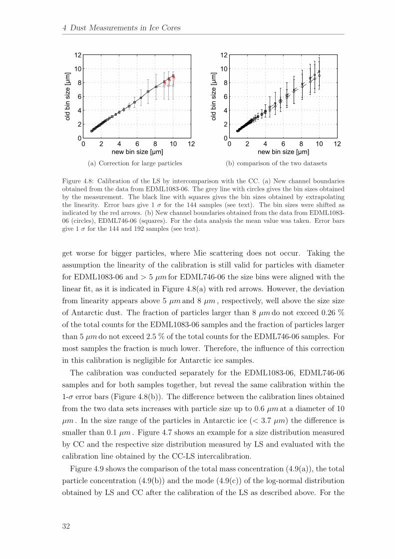
Figure 4.8: Calibration of the LS by intercomparison with the CC. (a) New channel boundariesobtained from the data from EDML1083-06. The grey line with circles gives the bin sizes obtainedby the measurement. The black line with squares gives the bin sizes obtained by extrapolatingthe linearity. Error bars give 1 σ for the 144 samples (see text). The bin sizes were shifted asindicated by the red arrows. (b) New channel boundaries obtained from the data from EDML1083-06 (circles), EDML746-06 (squares). For the data analysis the mean value was taken. Error barsgive 1 σ for the 144 and 192 samples (see text).
get worse for bigger particles, where Mie scattering does not occur. Taking the
assumption the linearity of the calibration is still valid for particles with diameter
for EDML1083-06 and > 5 μm for EDML746-06 the size bins were aligned with the
linear fit, as it is indicated in Figure 4.8(a) with red arrows. However, the deviation
from linearity appears above 5 μm and 8 μm , respectively, well above the size size
of Antarctic dust. The fraction of particles larger than 8 μm do not exceed 0.26 %
of the total counts for the EDML1083-06 samples and the fraction of particles larger
than 5 μm do not exceed 2.5 % of the total counts for the EDML746-06 samples. For
most samples the fraction is much lower. Therefore, the influence of this correction
in this calibration is negligible for Antarctic ice samples.
The calibration was conducted separately for the EDML1083-06, EDML746-06
samples and for both samples together, but reveal the same calibration within the
1-σ error bars (Figure 4.8(b)). The difference between the calibration lines obtained
from the two data sets increases with particle size up to 0.6 μm at a diameter of 10
μm . In the size range of the particles in Antarctic ice (< 3.7 μm) the difference is
smaller than 0.1 μm . Figure 4.7 shows an example for a size distribution measured
by CC and the respective size distribution measured by LS and evaluated with the
calibration line obtained by the CC-LS intercalibration.
Figure 4.9 shows the comparison of the total mass concentration (4.9(a)), the total
particle concentration (4.9(b)) and the mode (4.9(c)) of the log-normal distribution
obtained by LS and CC after the calibration of the LS as described above. For the
32

4.4 Calibration of the Laser Sensor
101 102 103 104
101
102
103
104
M L
S [n
g m
L−1]
M CC [ng mL−1]
(a) Mass concentration
103 104 105 106103
104
105
106
N L
S [n
g m
L−1]
N CC [ng mL−1]
(b) Number concentration
1 1.5 2 2.5 31
1.5
2
2.5
3
mod
e µ
LS [µ
m]
mode µ CC [µm]
(c) Mode μ
Figure 4.9: Comparison of the LS and CC measurements after the calibration. The dashed lineis the bisecting line as a guide to the eye. Clearly observable is the deflection in the numberconcentration caused by coincidences in the LS in higher concentrated samples.
mass concentration the two methods agree well (R = 0.93, slope = 1.04). For the
particle concentration the calibration does not work for high concentration above a
certain threshold. In this study a threshold of 350000 part · mL−1 was identified
as an upper limit for the validity of the calibration (R = 0.92, slope = 1.3). The
non-linearity of the calibration for higher concentrations is attributed to a higher
occurrence of coincidences in the LS, since the samples were diluted for the CC
measurements. For the mode, the calibration does not give a convincing relationship
between the two methods (R = 0.41), although no systematic difference in the mode
is found for LS and CC measurements after careful calibration. Irregular shape of
the particles, the fitting error and the coincidences in the LS, as mentioned for
the number concentration, are supposed to be the main reason for this mismatch.
Previous studies have already shown that different measurement techniques yield
different results depending on the shape of the particles ([Hayakawa et al., 1995b],
33

4 Dust Measurements in Ice Cores
[Hayakawa et al., 1995c], [Hayakawa et al., 1995a]). To achieve also a calibration
for the mode μ further more complex investigations have to be performed. In the
following, only the mode μ determined from the CC measurements is taken into
account, due to the more reliable measuring principle.
34
5 Dust Concentration and Size in the EPICA-DMLIce Core
5.1 Sampling Sites
The measurements were conducted on sections from the EPICA-DML ice core. The
drilling was performed at Kohnen Station located in DML (see Figure 5.1) from
2000 to 2006. The EPICA-DML ice core lies adjacent to the Atlantic sector on the
Antarctic plateau with a recent accumulation rate of 64 kg · m−2· year−1 ([Oerter
et al., 2000])). Details about the location are given in Table 5.1. The second core
drilled within EPICA is located at Dome C in the Indian sector on the Antarc-
tic plateau with an accumulation rate of only one third of EPICA-DML (recent
accumulation rate 25 kg · m−2· year−1 ([EPICA Community Members, 2004])).
5.2 Core Sections
For this study, two depth intervals of the EPICA-DML ice core were analyzed. From
each depth interval, the section indicated in Figure 4.2 with ”CFA” and parts from
the section indicated with ”Discontinuous samples” were available for analysis. On
the former the regular CFA-analysis ([Rothlisberger et al., 2000]) was performed,
including major ions (e.g. Ca2+, Na+ and NH+4 ), electrical conductivity, air content
and dust concentration using the LS. The latter was used for measurements of dust
concentration using the LS and the CC, electrical conductivity and air content.
The first section was chosen at the depth of 745-746 m corresponding to an age of
approximately 13200 yr BP ([Ruth et al., 2007b]) in the interval of the Antarctic cold
reversal (ACR, [Blunier et al., 1998]), herein after referred to as EDML746-04 (CFA-
position 75◦00’S, 00◦04’Ealtitude 2892 m a.s.l.mean annual surface temperature -44.6◦Cmean annual accumulation rate 64 kg · m−2· year−1 a
ice thickness 2774.15 mage at 87% of depth 150 000 a b
Table 5.1: Details of the EPICA-DML drill site. Data are taken from a [Oerter et al., 2004], b[Ruth et al., 2007b].
35

5 Dust Concentration and Size in the EPICA-DML Ice Core
DML
0°
80° 70° 60°
500 km0
Dome C
S-Pole
Berkner
Vostok
Taylor
Byrd
Neumayer
Figure 5.1: Overview about different drill sites and stations in Antarctica
cut) and EDML746-06 (Discontinuous samples-cut). The second section was taken
from a depth of 1082-1083 m corresponding to an age of about 25600 yr BP in the
last glacial ([Ruth et al., 2007b]), herein after referred to as EDML1083-04 (CFA-
cut) and EDML1083-06 (Discontinuous samples-cut). The measured parameters
were the same as for EDML746-04 and EDML746-06.
For EDML746-04 and EDML1083-04 the piece indicated with ”CFA” in Figure
4.2 and an additional 32×32 mm cut from the part indicated with ”discontinu-
ous samples” was used. The procedure for the measurements of EDML746-06 and
EDML1083-06 is described in Chapter 4.3, the procedure for the measurements of
EDML746-04 and EDML1083-04 is described by [Ruth, 2002].
5.3 Seasonal Variability of Glacial Dust
Figure 5.2 shows the dust concentration for the EDML depth of 1082-1083 m. In the
interval 1082.46 - 1082.67 m the depth resolution is 3 mm, hereafter referred to as
high resolution (HR). The rest of the core section was measured in 6 mm resolution.
The dust mass concentration varies between 100 ng · mL−1 and 10000 ng · mL−1 (300
ng · mL−1 and 11000 ng · mL−1 for HR) with a mean of 2000 ng · mL−1 (2900 ng ·mL−1 for HR). In terms of fluxes, this is in agreement with previous measurements at
Dome C (1000 ng · mL−1, [EPICA Community Members, 2004], accumulation rate
1.5 kg · m−2· year−1, [Schwander et al., 2001]) and Vostok (850 ng · mL−1 average
LGM, [Delmonte et al., 2002b], accumulation rate 1.2 kg · m−2· year−1, [Parrenin
et al., 2001]). The biggest variations are in the HR part (1082.4 m - 1082.7 m). That
36
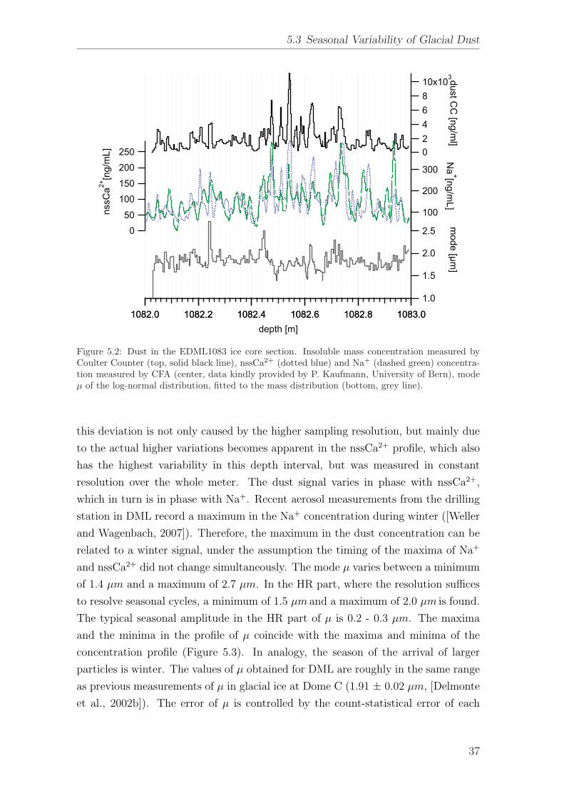
5.3 Seasonal Variability of Glacial Dust
2.5
2.0
1.5
1.0
mode [µm
]
1083.01082.81082.61082.41082.21082.0depth [m]
10x103
86420
dust CC
[ng/ml]
250200
150100
500
nssC
a2+[n
g/m
L]
1083.01082.81082.61082.41082.21082.0
300
200
100
Na
+[ng/mL]
Figure 5.2: Dust in the EDML1083 ice core section. Insoluble mass concentration measured byCoulter Counter (top, solid black line), nssCa2+ (dotted blue) and Na+ (dashed green) concentra-tion measured by CFA (center, data kindly provided by P. Kaufmann, University of Bern), modeμ of the log-normal distribution, fitted to the mass distribution (bottom, grey line).
this deviation is not only caused by the higher sampling resolution, but mainly due
to the actual higher variations becomes apparent in the nssCa2+ profile, which also
has the highest variability in this depth interval, but was measured in constant
resolution over the whole meter. The dust signal varies in phase with nssCa2+,
which in turn is in phase with Na+. Recent aerosol measurements from the drilling
station in DML record a maximum in the Na+ concentration during winter ([Weller
and Wagenbach, 2007]). Therefore, the maximum in the dust concentration can be
related to a winter signal, under the assumption the timing of the maxima of Na+
and nssCa2+ did not change simultaneously. The mode μ varies between a minimum
of 1.4 μm and a maximum of 2.7 μm. In the HR part, where the resolution suffices
to resolve seasonal cycles, a minimum of 1.5 μm and a maximum of 2.0 μm is found.
The typical seasonal amplitude in the HR part of μ is 0.2 - 0.3 μm. The maxima
and the minima in the profile of μ coincide with the maxima and minima of the
concentration profile (Figure 5.3). In analogy, the season of the arrival of larger
particles is winter. The values of μ obtained for DML are roughly in the same range
as previous measurements of μ in glacial ice at Dome C (1.91 ± 0.02 μm, [Delmonte
et al., 2002b]). The error of μ is controlled by the count-statistical error of each
37

5 Dust Concentration and Size in the EPICA-DML Ice Core
2.2
2.0
1.8
1.6
1.4
mod
e [µ
m]
1082.651082.601082.551082.50
depth [m]
1.2x10⁴
1.0
0.80.60.4
0.20.0
dust CC
[ng/mL]
Figure 5.3: Dust mode μ in the Glacial in different resolution: 3 mm resolution (black solid line)and 3 cm resolution (grey dashed line).
size bin√
N (with the number of counts N) and the interval chosen for fitting. The
influence of the counting statistics was determined by a Monte Carlo technique as
follows: 1000 size spectra were calculated, where the counts in each size bin were
varied, that the mean of the 1000 values for this size bin equaled the measured value
N and the 1 σ interval the count-statistical error√
N for this size bin. This was
done for all size bins yielding 1000 size spectra. The mode obtained by performing
a log-normal fit on all those spectra varied within 1 σ of less than 0.02 μm for the
glacial samples. The influence of the interval chosen for fitting was determined by
changing the fitting interval. The range for reasonable values for μ by changing the
range of the fitting interval was 0.05 μm and thus the dominant error.
To investigate the influence of the seasonality the mode of 3 mm resolution sam-
pling intervals (μ3) is shown in comparison with the mode fitted on 30 mm resolution
sampling intervals (μ30) (Figure 5.3). To obtain μ30 ten consecutive samples were
summed up and afterwards the log-normal function was fitted on the mass distribu-
tion. The mean value for μ30 emerges as 1.88 ± 0.15 μm .
Interestingly, μ30 is always higher than the mean of μ3 in the respective interval.
This observation can be explained by combining two findings. First, maxima and
minima in mass and mode are in phase and second, mass concentration changes
within one year between maxima and minima on average by a factor of about 7.6.
By measuring samples covering several years, the obtained mode is dominated by
events of high mass input and represents in glacial time the size distribution during
winter.
38

5.4 Dust Transport to DML in the Last Glacial
2 2.5 3 3.5 4
0.3
0.5
0.7
µcold
/µwarm
= 0.75
µcold
/µwarm
= 0.85
µcold
/µwarm
= 0.9
µAir
= µIce
µ0 [µm]
t cold
/t war
m
(a) no correction for deposition
2 2.5 3 3.5 4
0.3
0.5
0.7µ
cold/µ
warm = 0.94
µcold
/µwarm
= 0.84
µcold
/µwarm
= 0.66
µAir
< µIce
µ0 [µm]
t cold
/t war
m
(b) correction for deposition
Figure 5.4: Seasonal changes in transport efficiency for glacial dust depending on the mode of theinitial dust at the source.
5.4 Dust Transport to DML in the Last Glacial
In the following chapter the observed changes in dust concentration and size are
used to quantify the contribution of changes inferred by transport and the source.
Invented by [Ruth, 2002] and improved by [Fischer et al., 2007b] a one dimensional
model to describe the dust transport to Greenland ice cores is used to quantify the
changes in transport time and efficiency to DML (see also chapter 2.5). It yields a
relation between dust size and effective transport time (equation 2.4).
logμI
air
μIIair
= logμI
air
μ0
(1 − μIIair
2
μIair
2
tII
tI)
or
tII
tI= (1 −
logμI
air
μIIair
logμI
air
μ0
) · μIair
2
μIIair
2 (5.1)
In high resolution the ratio between maxima and minima in the mode varies in
the Glacial between 0.75 and 0.9 with a mean of 0.85 ± 0.06. Equation 5.1 with
the mode of the initial dust at the source of 2.5 μm ([Schulz et al., 1998]) yields an
effective transport time ratio between 0.4 and 0.7. Figure 5.4(a) illustrates the effect
of a variation in μ0. A larger μ0 than the assumed 2.5 μmwould not have a large
effect on tII
tI, whereas a smaller μ0 would have a larger effect. Equation 2.4 describes
only the changes of the mode in the atmosphere. Instead, the values used here are
measured in ice. In DML, where aerosol is deposited by wet and dry processes, the
enrichment in larger particles due to dry deposition onto the snow has to be taken
39

5 Dust Concentration and Size in the EPICA-DML Ice Core
into account. The relation between dust size distribution in air Vice(logd) and in ice
Vice(logd) is described by [Fischer et al., 2007b] with
Vice(logd) = Vair(t, logd)[kd2 + εA] (5.2)
Therewith the relation 2.4 changes to
logμI
ice
μIIice
= [logμI
ice
μair,0
− 2kln10log2σ0μII
ice2
kμIIice
2+ εAII
ice
] · [tII
tIμII
air2
μIair
2 − 1]+ (5.3)
2kln10log2σ0 · [ μIice
2
kμIice
2+ εAI
ice
− μIIice
2
kμIIice
2+ εAII
ice
]
The mode corrected according to Equation 5.3 varies between 1.4 and 1.7, with
changes in the ratioμI
air
μIIair
between 0.66 and 0.94 with a mean of 0.83. For this
calculation the glacial accumulation A = 30 kg · m−2· year−1 ([Ruth et al., 2007a])
was assumed to be constant throughout the year and k = 83 μm−1s−1 and ε = 106
was used as by [Ruth et al., 2003]. Figure 5.4(b) shows the effective transport time
changes using this relation, depending on the initial mode at the source μair,0. The
curves for the uncorrected data (Figure 5.4(a)) are more bent, indicating a larger
consequence of a change in the initial mode on the calculated effective transport time.
The variation in accumulation corrected ratiosμI
air
μIIair
is larger than in the uncorrected
ratios, but the mean effective transport time change is 0.6 and does not alter after
correcting for deposition processes. However, the variation becomes larger ( tcold
twarm=
0.3 - 0.85). In the following tcold
twarm= 0.6 will be used for the effective transport time
change ratio.
Now we can estimate the influence of changes in transport and source on the dust
concentration in the ice core.
If we apply equation 2.1
Cair(t) = Cair(0)e−tτ
for a warm stage corresponding to summer and a cold stage corresponding to
winter conditions, they are related to each other as follows:
Cair(twarm)
Cair(tcold)=
Cair(0)warm
Cair(0)cold
· e− twarmτ
+tcold
τ (5.4)
Assuming the atmospheric transport time τ as constant throughout the year and
using tcold
twarm≈0.6 and Cair(tcold)
Cair(twarm)≈ 7.6, which is the mean value of the ratio be-
tween the maximum and minimum concentrations in the HR-part of EDML1083,
the relations emerges as
40

5.4 Dust Transport to DML in the Last Glacial
Cair(tcold)
Cair(twarm)=
Cair(0)cold
Cair(0)warm
· e0.4· twarmτ = 7.6. (5.5)
To calculate Cair(0)cold
Cair(0)warm, twarm
τhas to be estimated. There are only few studies
about the atmospheric residence time of dust in the last Glacial. Measurements
of modern global atmospheric residence time of dust do not exist ([Zender et al.,
2003]). Model estimates for modern atmospheric residence time vary between 2.7
days ([Mahowald et al., 2006]) and 7.1 days [Ginoux et al., 2001] with most of the
estimates between 4 and 5.5 days ([Luo et al., 2003], [Miller et al., 2006], [Zender
et al., 2003], [Tegen and Fung, 1994]). However, glacial residence times are longer.
The increase varies from very slight increases of 5 % ([Lunt and Valdes, 2002]) to
higher values of 30 % ([Werner et al., 2002]). This leads to glacial residence times of
4.2 - 7.1 days based on a modern residence time of 4 - 5.5 days. For the transport time
no direct measurements in the Glacial are available. Backward trajectory studies for
modern times yield transport times from Patagonia to DML of 5 - 10 days except
events accompanied by very high snow fall, which are shorter ([Reijmer and van den
Broeke, 2001]). Even if similar data is not available for glacial climate, it might
serve as a rough estimate for transport times during the Glacial. Taking 5 days as
a lower limit for the summer transport time (implying a winter transport time of 3
days) this would lead to a source ratio Cair(0)warm
Cair(0)coldbetween 4.6 (for τ =4 days) and 5.3
(for τ =5.5 days). This estimation means, that maximal 60 - 70 % of the subannual
dust concentration changes can be explained by the source. Assuming 10 days as an
upper limit for the summer transport time (implying a winter transport time of 6
days) would lead to a source ratio Cair(0)warm
Cair(0)coldbetween 2.8 (for τ =4 days) and 3.7 (for
τ =5.5 days). Under this conditions 37 - 49 % of the subannual dust concentration
changes can be explained by the source. This conclusion implies depending on
transport time estimations, 30 - 63 % of the seasonal dust concentration changes
must be explained by transport changes.
On the other extreme, to explain 100 % of the subannual dust concentration
changes by transport only, implies values for twarm between 20 days (for τ =4 days)
and 28 days (for τ =5.5 days) and for tcold between 12 days (for τ =4 days) and 17
days (for τ =5.5 days). This is up to a factor of 3 higher, than the estimates by
[Reijmer et al., 2002]. Further, LGM backward trajectory studies have to be run
using high resolution atmospheric transport models to validate this reasoning.
Seasonal changes in dust sources are observed by satellite imagery for recent times
([Prospero et al., 2002]) and are very likely to occur during the Glacial as well caused
by changing wind speed, vegetation cover, soil moisture or changes in the areas,
which supply the source with erodible material.
41
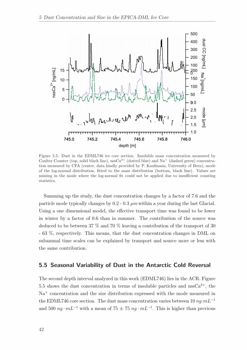
5 Dust Concentration and Size in the EPICA-DML Ice Core
3.0
2.5
2.0
1.5
1.0
mode [µm
]
746.0745.8745.6745.4745.2745.0depth [m]
500
400
300
200
100
0
dust CC
[ng/mL]
15
10
5
0
nssC
a2+[n
g/m
L]
746.0745.8745.6745.4745.2745.0
200
150
100
50
0
Na
+[ng/mL]
Figure 5.5: Dust in the EDML746 ice core section. Insoluble mass concentration measured byCoulter Counter (top, solid black line), nssCa2+ (dotted blue) and Na+ (dashed green) concentra-tion measured by CFA (center, data kindly provided by P. Kaufmann, University of Bern), modeof the log-normal distribution, fitted to the mass distribution (bottom, black line). Values aremissing in the mode where the log-normal fit could not be applied due to insufficient countingstatistics.
Summing up the study, the dust concentration changes by a factor of 7.6 and the
particle mode typically changes by 0.2 - 0.3 μmwithin a year during the last Glacial.
Using a one dimensional model, the effective transport time was found to be lower
in winter by a factor of 0.6 than in summer. The contribution of the source was
deduced to be between 37 % and 70 % leaving a contribution of the transport of 30
- 63 %, respectively. This means, that the dust concentration changes in DML on
subannual time scales can be explained by transport and source more or less with
the same contribution.
5.5 Seasonal Variability of Dust in the Antarctic Cold Reversal
The second depth interval analyzed in this work (EDML746) lies in the ACR. Figure
5.5 shows the dust concentration in terms of insoluble particles and nssCa2+, the
Na+ concentration and the size distribution expressed with the mode measured in
the EDML746 core section. The dust mass concentration varies between 10 ng·mL−1
and 500 ng ·mL−1 with a mean of 75 ± 75 ng ·mL−1. This is higher than previous
42

5.5 Seasonal Variability of Dust in the Antarctic Cold Reversal
1
10
100
1000
dust
CC
[ng
mL−1
]
745 745.2 745.4 745.6 745.8 746
1.4
1.6
1.8
2
2.2
2.4
dust
siz
e [µ
m]
depth [m]
Figure 5.6: Dust in the EDML746 ice core section. Top: Mass concentration, bottom: size distri-bution expressed by Mean mass diameter (MMD) grey dashed line and mode in black solid line.The vertical lines indicate coinciding maxima or minima in mass and mode (red solid lines) andin mass and MMD (blue dashed lines).
measurements in other Antarctic ice cores (EPICA Dome C 25 ng ·mL−1, KMS 25
ng ·mL−1, Dome B 46 ng ·mL−1 ([Delmonte et al., 2004b])). Even in terms of fluxes
the highest values are found in DML (EPICA-DML: 12.5 ng · cm−2yr−1, EPICA
Dome C: 8.3 ng · cm−2yr−1, KMS: 8.3 ng · cm−2yr−1, DOME B: 9 ng · cm−2yr−1).
This difference can be explained by the closer proximity of DML to the dust source
(see Chapter 6 and [Delmonte et al., 2004a]). The profile of the insoluble particles
closely follows the nssCa2+-profile. Unlike in Glacial times the Na+ and nssCa2+-
profile are not well correlated. Therefore it is hard to determine the timing of the
dust maximum.
The particle mode does not follow the mass as closely as in glacial ice. It varies
between 1.4 μm and 2.4 μm , but shows two cluster around 1.75 μm and 2.05 μm .
The maxima of the mode usually are in line with dust concentration maxima. The
variance of the mode induced by changing the fitting range is the same as for glacial
samples (± 0.05 μm ). The count-statistical error, obtained as described in Section
5.3 is up to 0.1 μm and therewith the controlling error for the lower concentrated
samples from the ACR. In any case, values for the mode have to be considered very
carefully, since the limited counting statistics did not allow reliable determination of
43

5 Dust Concentration and Size in the EPICA-DML Ice Core
the mode for all samples. To get a continuous record also in the mode, a log-normal
fit was performed on averages of 10 consecutive samples as explained in Section 5.3.
Seasonal resolution could not be obtained by this average but a reliable mean value
for the mode could be calculated as 1.96 ± 0.13 μm . This value is only slightly
higher than the dust size at Dome C ice core (1.94 μm± 0.17 μm ([Delmonte et al.,
2002b])). A higher value in DML than at Dome C is expected due to the closer
proximity to the source in South America. One possible explanation for the small
difference could be different transport routes from the source to DML and Dome C.
Here again, one has to keep in mind that the values both in DML and at Dome C
are governed by the high dust mass concentration events.
Additionally to the mode, the mean mass diameter (MMD) was calculated. It
shows a reasonable correlation with the mode: R=0.74, slope 1.03 for ACR and
R=0.93, slope 1.26 for glacial dust. The difference in R is probably due to better
statistics in glacial ice, the difference in the slope indicates a higher skewness of
the glacial distributions towards larger sizes. The advantage of the MMD is the
possibility to calculate it even for low-concentration samples, where the low counting
statistics does not allow a determination of the mode. In order to investigate if the
seasonal cycle is as pronounced as in glacial ice, Figure 5.6 shows mass, MMD and
mode. The correlation between the logarithmic mass and the mode is weak (R=0.3).
The calculated correlation between MMD and mass is only slightly higher (R=0.33).
However, even if the correlation is low, many of the maxima and minima of the mass
and mode (MMD) coincide as indicated with red (blue dashed) lines in Figure 5.6.
5.6 Dust Transport to DML during the Antarctic Cold Reversal
The above described coincidences between mode μ and mass point to a relationship
between mass concentration and size, that allows to apply the linear transport model
described in Section 5.4 also in the ACR. Since consecutive clear seasonal cycles
could not be obtained in the ACR, selected slices of the mass concentration and
size profile are used instead. Those parts of the profile, where an uninterrupted
transition from a higher to a lower mass concentration coincides with a transition
from larger to smaller values for the mode and vice versa, are used in the following
to estimate changes in the effective transport time during the year. 16 of those
slices were identified. The mean value for the respective larger mode is 2.07 ±0.16 μm , for the respective smaller mode 1.74 ± 0.15 μm , the difference between
maximum and minimum is generally 0.2 - 0.35 μmwith three outliers of 0.6 μm .
The corresponding maxima and minima in the mass concentrations are 260 ± 160
ng ·mL−1 and 74 ± 45 ng ·mL−1. For each pair of large and small mode the change
44

5.6 Dust Transport to DML during the Antarctic Cold Reversal
in the effective transport time tII
tIcan be calculated using Equation 5.1
tII
tI= (1 −
logμI
air
μIIair
logμI
air
μ0
) · μIair
2
μIIair
2
The mean effective transport time ratio between summer and winter deduced from
the above mentioned 16 events is 0.4 ± 0.15. Here like for the calculation of the
Glacial a μ0 of 2.5 μmwas assumed ([Schulz et al., 1998]). 13 of these 16 events
give very similar effective transport time ratios of 0.46 ± 0.07, the other 3 are lower
with 0.12 (twice) and 0.16.
Now the changes in the dust concentration in the EPICA-DML ice core can be
divided in changes caused by the source and changes caused by transport for the
ACR as well (Equation 5.4).
Cair(twarm)
Cair(tcold)=
Cair(0)warm
Cair(0)cold
· e− twarmτ
+tcold
τ
As in the Glacial, τ is assumed to be constant throughout the year. With tcold
twarm≈
0.4 and Cair(tcold)Cair(twarm)
≈ 3.5 the relation emerges as
Cair(tcold)
Cair(twarm)=
Cair(0)cold
Cair(0)warm
· e0.6· twarmτ ≈ 3.5 (5.6)
As discussed in Section 5.4 model predictions for τ vary from 4 to 5.5 days. Modern
transport times based on back trajectory calculations are 5-10 days ([Reijmer et al.,
2002]). These values will be used for the ACR as well. During summer the transport
time is 2.5 times longer than during winter. Assuming 10 days of summer transport
time the second term in Equation 5.6 describing changes in transport varies between
≈ 3 (for τ = 5.5 days) and 4.5 (for τ = 4 days). This means, depending on the
assumed transport time and atmospheric residence time τ , between 70 and 100 % of
the dust variation in DML can be explained by transport changes during the ACR.
The remaining less than 30 % are attributed to the source. Assuming a transport
time less than 10 days for summer, the contribution of the source rises. A longer
transport time would lower the contribution of the source.
Modern back trajectory calculations indicate a shorter transport time from South
America to DML during autumn (March - April - May) and spring (September -
October - November) than during summer (December - January - February). Winter
(June - July - August) trajectories are similar to those in spring and autumn, but
have a slightly more northern origin ([Reijmer et al., 2002]). This is explained by
the authors by a weaker cyclonic activity during summer. This is in line with the
results of the present work for the ACR.
45

5 Dust Concentration and Size in the EPICA-DML Ice Core
Glacial ACRmean mass concentration [ng · mL−1] 2000 70factor of mean subannual mass variation 7.6 3.5size (mode [μm]) 1.4 - 2.7 1.4 - 2.4mean size (determined in samples coveringseveral years [μm])
1.88 ± 0.15 1.96 ± 0.13
typical subannual mode shift [μm] 0.2 - 0.3 0.2 - 0.35contribution source [%] 37 - 70 < 30factor of mean subannual mass variation ex-plained by transport
2.8 - 5.3 3 - 4.5
contribution transport [%] 63 - 30 70 - 100
Table 5.2: Variation of dust parameter during glacial times and during the ACR on subannualtime scales.
Summing up this section, the dust concentration during the ACR changes by a
factor of ≈ 3.5 with some larger excursions. The mode μ could not be determined
for all samples, especially those with low dust concentration, due to insufficient
counting statistics. For all other samples the mode generally varies between maxima
and minima by 0.2 - 0.35 μm . Using a simple transport model the transport time
was found to be lower by a factor of 0.4 in winter than in summer. 70 - 100 % of
the dust concentration changes in the ACR could be explained by transport, the
remaining less than 30 % are attributed to changes in the source.
5.7 Comparison of Glacial and Antarctic Cold Reversal
After investigating in detail two depth intervals from the EPICA-DML ice core, the
variability of dust size and concentration on Glacial-Interglacial timescales will be
discussed in the following section.
The main characteristics of dust concentration and size during the ACR and the
Glacial are summarized in Table 5.2. The mean mass concentration is higher during
the Glacial than during the ACR by a factor of ≈ 28. The respective nssCa2+
concentration ratio is ≈ 25 ([Fischer et al., 2007a]). A higher ratio of insoluble dust
particle between Glacials and Interglacials compared to the nssCa2+ ratio is already
observed by [Ruth et al., 2007a]. One possible explanation for this discrepancy could
be a change in the mineralogical composition of the dust in the EPICA-DML ice
core during the transition from the Glacial to the Holocene. This could be caused
by a change in the source of the dust reaching DML. Another possibility to explain
the higher ratio of insoluble dust compared to nssCa2+ could be a different recovery
efficiency for nssCa2+ in glacial ice and ice from the ACR.
The seasonal dust concentration changes are more than a factor of 2 higher during
46

5.7 Comparison of Glacial and Antarctic Cold Reversal
the Glacial than during the ACR. During the ACR almost the entire dust concen-
tration changes of 3.5 can be explained by transport (Section 5.6). The variability
inferred by the transport are in the same range during the Glacial as during the ACR.
However, to explain the observed seasonal dust concentration changes an additional
contribution from the source is required during the Glacial. The contribution from
the source has to be approximately as large as the contribution explained by trans-
port. The mean values for μ during Glacial and ACR are in agreement within the
1-σ interval, with a slightly higher value for the ACR. The typical shift of μ during
the year is approximately the same during the Glacial and the ACR.
Accepting the values given in Table 5.2 for the mean size determined in samples
covering several years at face values for the dust size during the Glacial at the
ACR, the change in effective transport time can be estimated. Again, the simple
conceptual transport model described in Section 2.5 is used for the calculation,
yielding the relations
tACR
tGlacial= (1 −
logμGlacial
air
μACRair
logμGlacial
air
μ0
) · μGlacialair
2
μACRair
2
and
Cair(tACR)
Cair(tGlacial)=
Cair(0)ACR
Cair(0)Glacial
· e−tACRτACR
+tGlacialτGlacial
Note, the atmospheric residence time τ does not have to be constant. Model
simulations yield a longer residence time τ of up to 30 % in the Holocene than in
the Glacial ([Lunt and Valdes, 2002], [Werner et al., 2002]). However, assuming in
a first (unrealistic) step τ = τACR = τGlacial constant between Glacial and ACR ,
with μACR = 1.96 μm , μGlacial = 1.88 μm , the transport term e− tACR
τACR+
tGlacialτGlacial is
calculated ≤ 1. This indicates a possibly intensification of the transport during
the Glacial-Interglacial transition. By assuming in a second more realistic step a
longer atmospheric dust residence time during the Glacial than during the ACR,
the factor given by the transport term would decrease even more indicating an even
stronger intensification of the transport from the Glacial to the ACR. There are
previous publications supporting this findings. A pollen and diatom record obtained
out of a sediment core in southern South America (51◦58’ S, 70◦23’ W) reveals
relatively calm winds during the late Glacial and an increase of the wind speed after
15440 yr BP ([Wille et al., 2007]).[Toggweiler and Russell, 2008] argues, that lower
atmospheric CO2 concentrations during LGM cause smaller temperature gradients
in the middle of the atmosphere between low and high latitudes. This temperature
gradient drives the westerly winds, which therefore would have increased during the
47

5 Dust Concentration and Size in the EPICA-DML Ice Core
Glacial-Holocene transition. If transport would be indeed less effective during the
Glacial than during the ACR, more than the observed dust concentration difference
between Glacial and ACR has to be explained entirely by the source, implying a
large increase of the source intensity. A record of three lake sediment cores from Lago
Cardiel (49◦ S, 71◦ W) shows a significant increase in the lake level coinciding with
the low dust concentration between 11600 and 11500 yr BP in Antarctic ice cores
([Gilli, 2003]). The authors explain the lake level increase with a strong positive
hydrological balance at that time and an accompanying higher washout of dust
from the atmosphere in the source region resulting in a lower dust concentration in
Antarctica.
A combination of changes in glacial outwash, aridity and wind speed in the source
are suggested to be mainly responsible for the required weakening of the source
during the transition from Glacial to the Holocene ([Fischer et al., 2007a]). The shelf
exposed adjacent to Argentina in the Atlantic is ruled out as a major contribution
to the glacial dust source by [Wolff et al., 2006].
Based on nssCa2+-fluxes in the EPICA-DML and EPICA-Dome C ice cores [Fis-
cher et al., 2007a] found, that the observed changes in dust fluxes between Holocene
and Glacial of 1-2 orders of magnitude predominantly reflect changes in source
strength. The results of the presented work suggest actually an extend of the findings
by [Fischer et al., 2007a], that the source intensification could have been stronger
than the Glacial-Interglacial dust concentration changes in the EPICA-DML ice
core. There, one has to keep in mind, that in this study Glacial-ACR changes are
presented and [Fischer et al., 2007a] addresses Glacial-Holocene changes.
Admittedly, the values obtained for μ are mean values for one meter during each
time interval representing only one data point each in the Glacial and the ACR. The
seasonal as well as the interannual variability of μ is much larger than the difference
between the obtained ACR-Glacial difference. To confirm the obtained findings on
more depth intervals dust size measurements have to be performed.
[Delmonte et al., 2004b] explains observed changes of dust size during the transi-
tion from the last Glacial in the Indian sector of Antarctica with different pathways
for different size classes. A gradual change of the eccentricity of the polar vortex
is proposed to govern the transport of particles of different sizes onto the Antarc-
tic plateau. Larger particles are transported over the lower troposphere, whereas
smaller particles are transported in higher altitude and dominated by the subsidence
of air masses over the east Antarctic ice sheet. This hypothesis was derived based
on measurements in ice cores in the Indian sector of Antarctica and may therefore
not be valid for DML. These regional distinctions indicate, that the different drill
48

5.7 Comparison of Glacial and Antarctic Cold Reversal
sites of the EPICA-DML and the EPICA-Dome C ice cores, even if they are both
located on the East Antarctic plateau, appear to be influenced by different changes
during the Glacial-Interglacial transition.
49

6 Sources of Dust in Dronning Maud Land
The sources of dust in the EPICA-DML ice core are identified by a new approach
using REE. In a first step the REE fingerprints are determined in samples from the
PSAs. Afterwards the REE fingerprints in the EPICA-DML ice core sample are
determined and compared to the REE fingerprints in the PSA samples.
6.1 Measurements of Rare Earth Elements
Due to the large differences in REE concentration and different matrices in the PSA
and ice core samples two different procedures were applied to the two sets of samples.
Figure 6.1 gives an overview of the two processing procedures. Processing and
measurement of the PSA samples was performed at AWI and is described in Section
6.1.1. The EPICA-DML samples were processed and measured at the University of
Venice. A detailed description is given in Section 6.1.2. An intercomparison study
proving the consistency of both systems will be submitted soon ([Dick, et al. in
preparation]).
6.1.1 Samples from the Potential Source Areas
The samples collected from the PSAs span a wide size spectrum differing from
sample to sample. For the analysis only the < 5 μm fraction was used. This
corresponds to the typical size of the particles found in Antarctic ice cores (see
Chapter 5, [Delmonte et al., 2002a], [Delmonte et al., 2004a]). The bulk of the
sample (a few grams) was poured into 45-50 mL of ultra pure water. After 10
minutes of ultra sonication the sample was left to separate by settling due to Stokes
law. The supernatant was taken with a pipette and checked with the CC to achieve
a fraction of 95 % of the total number of particles in a size range < 5 μm. This
aliquot may also include the soluble fraction of REE dissolved from coarser particles
with a size > 5 μm. Due to the low solubility of the REE ([Humphris, 1983]),
this contribution can be neglected. The size separation was performed within a
cooperation with the University of Milan, Italy. Most of the samples were kindly
provided by Barbara Delmonte. For detailed information about the samples see
[Delmonte, 2003] and [Delmonte et al., 2004a].
50

6.1 Measurements of Rare Earth Elements
Sample inlet
AWI: MCN 6000
(Cetac), and a
100 μl PFA Nebulizer
UVe:ARIDUS
Output
Signal
Processing
Vacuum system
Detector
Both:
photomultiplyer
Mass analyser
AWI: Quadrupol
Uve: Sectorfield
Ion source
Both: Plasma
SamplesPSA-samples:
full acid digestion
ice core samples:
HN03 acidification
Figure 6.1: Schematic overview of the two processing and measurement setups used in this work.PSA samples are treated with a full acid digestion and measured using the ICP-QP-MS at AWI.Ice core samples are acidified with 1 % HNO3 and measured at the University of Venice (UVe)using the ICP-SF-MS.
The aliquots containing the dust fraction < 5 μm are treated with a full acid
digestion. The samples added with HNO3 (twofold distilled, 65 %, p.A., Merck),
HF (distilled, 40 %, suprapur, Merck) and H2O2 (suprapur, Fa. SCP Science) are
pressurized using polytetrafluoroethylen (PTFE) beakers to completely solubilize
the sample matrix. The full digestion protocol is given in Appendix A.
At AWI all lab ware used to contain the samples, standards and used to prepare
the solutions are cleaned following the procedure given in Appendix B.1. The diges-
tion and the measurement of the samples are performed under a clean bench (US
Class 100) in the clean room facilities at AWI, classified as US Class 10000, but
presently U.S. Class 100-1000 is achieved. To each sample 10 μg·L−1 Rh are added
to provide an internal standard to correct for instrumental drift during the measure-
ments. Possible interferences of the Rh standard from ArCu, RbO and Pb2+ were
not found to be significant. In any case through an interference on the Rh signal
all REE concentration would be subjected to the same error, that vanishes, when
considering relative changes among REE. Only the absolute concentration, which is
51

6 Sources of Dust in Dronning Maud Land
ICP-QP-MS ICP-SF-MSICP-MSRF Power [W] 1350 1250Plasma gas [L·min−1] 15 15.5Auxiliary gas [L·min−1] 0.8 1.8Nebulizer gas [L·min−1] 0.62 0.8-1.1Nebulizer (with desolvatisation) MCN 6000 Aridus ISweep gas [L·min−1] 2.35 3.4 - 4.15Nitrogen [L·min−1] 12 15T (spray chamber) [◦C] 110 95T (desolvating unit) [◦C] 160 175sample uptake [μ·min−1] 100 100Data aquisitionIsotopes analyzed ≈ 40 19Replicates 3 40Integration time [s] 0.1Sweeps 20Measuring time per sample [min] 7Oxids [%] 0.03Double charged Ions [%] 5.7
Table 6.1: Settings of the two ICP-MS used for ice core samples and PSA samples.
not discussed in this work, would be effected. Therefore, interferences on Rh do not
affect the result of this work, anyways.
Blanks were prepared using ultra pure water, treated by the same procedure as
the samples and measured regularly during data collection. The median of the blank
values is subtracted from the sample concentration. The blank samples contain less
than 0.5 % of the mean concentration in the samples and less than 10 % of the
concentration in the lowest concentrated sample. The blanks for the REE are given
in Appendix B.2. Calibration standards were prepared from a 10 μg · L−1 multi-
element stock solution (Multielement Calibration Standard 2 and 3, Perkin-Elmer).
The measurements were performed with a ICP-QP-MS ELAN 6000 built by Perkin
Elmer/Sciex 1997 coupled with a micro concentric nebulizer and a desolvation unit
MCN-6000 built by Cetac. The MCN-6000 is equipped with a heated membrane to
separate the aerosol and the solvent. Thus the oxygen of the water available for oxid
formation is minimized yielding an oxid formation rate for the REE of about 0.02
%. The uptake rate of sample is 100 μL · min−1. The mean sensitivity obtained
during the measurements is 490000 ± 200000 counts per second for a 10 μg · L−1
Rh solution. Instrumental conditions and measurement settings are summarized in
Table 6.1.
52

6.1 Measurements of Rare Earth Elements
- La Ce Pr Nd Sm Eudetection limit [ppt] 0.303 0.523 0.087 0.296 0.055 0.075
melt head blank [ppt] 0.353 0.639 0.085 0.267 0.077 0.026acid blank [ppt] 0.5509 0.9769 0.0837 0.2625 0.0653 0.0159
Gd Tb Dy Ho Er Tm Yb Lu0.044 0.018 0.039 0.019 0.029 0.022 0.034 0.0230.075 0.019 0.044 0.009 0.024 0.006 0.02 0.010.0281 0.0041 0.0221 0.0046 0.0133 0.0032 0.0127 0.0024
Table 6.2: Detection limits and procedural blanks of the REE measurements in ice core samples.Calculations are described in the text.
6.1.2 Ice Core Samples
The ice core samples were taken from the innermost part of the core assigned to the
CFA-analysis (see Figure 4.2 in Chapter 4). They were decontaminated using the
melt head (Figure 4.1). Thus only the inner uncontaminated ice was used for the
analysis. For the first time the sample decontamination using the melt head was
performed for REE measurements. One line from the melt head filled 15 mL PS
vials, that were also used for ion chromatography analysis (IC) providing continuous
1 m averages (Figure 4.1). These samples were immediately frozen after filling,
once melted to take an aliquot for the IC and refrozen immediately afterwards. In
a previous study, using a chiseling method, the ice core was decontaminated by
removing ice in different layers from the outside to the inside. It was proved in that
study, that the inner part of the ice core is not contaminated in REE by the drilling
fluid ([Gabrielli et al., 2006]).
At least 24 h before the REE measurements, the samples were melted, filled
into polypropylene vials (Greiner Bio-One), acidified with 100 μL HNO3 (twofold
distilled, p.a. 65 %, Fa. Merck) per 10 mL sample and afterwards kept frozen until
the measurement. All sample handling was performed under class 100 clean room
conditions. The cleaning scheme of the vials is given in Appendix B.1.
The measurements of the REE in the ice core samples were performed at the
University of Venice, Italy, with an ICP-SFMS (Element2, Thermo Finnigan MAT,
Bremen) coupled with a microflow/desolvation sample introduction system (Aridus,
Cetac Technology). The Aridus consists of a microflow PFA nebulizer, a heated
PFA spray chamber and a heated microporous PTFE tabular membrane. Interfer-
ences induced by oxides were highly reduced by this setup. The measurements were
performed in low resolution mode with a nominal mass resolution of Δmm
≈ 400. The
sample uptake by the system was 100 μL · min−1. The maximum sensitivity in low
53

6 Sources of Dust in Dronning Maud Land
resolution mode (LRM) was 3 · 106 counts · s−1 for a 1 μg · L−1 Indium solution.
The instrument stability was checked every seventh sample with a 1 μg · L−1 Indium
solution. Additionally 129Xe and 131Xe was measured. Xe is included as an impurity
in the used Argon and Nitrogen. If needed, the measurements are corrected for in-
strumental drift using the 129Xe signal. The use of an internal standard like for the
samples from the PSA was not possible due to the much lower REE concentration
in the ice core samples associated with a much higher risk of contamination by the
internal standard.
The blanks of the acid and the vials were determined with a series of blank
samples with decreasing acidity (Figure B.1). The blanks of the CFA-melt head
were determined with artificial ice bars cut out of artificial ice cores made of ultra
pure water. These artificial ice bars were handled in the same way as the samples.
Blanks were determined as the median of 10 samples. Both blank level values and
detection limits are given in Table 6.2. The melt head blank is in the same range
as the acid blank. The detection limit was calculated as three times the standard
deviation of 10 replicates of 1 % HNO3 in ultra pure water.
For La, Ce, Pr, Nd, Sm, Gd, and Dy measured in the EPICA-DML ice core
samples from Holocene lie three to ten times above the detection limit and 10-200
times for glacial samples. For Tb, Ho, Er, and Yb the concentrations lie in the range
of the detection limit for Holocene samples and 5-200 times above the detection limit
for glacial samples. For Eu, Tm and Lu the concentrations lie below the detection
limit for most of the Holocene samples and about ten times above the detection
limit for glacial samples. The total blank (melt head blank) was subtracted from
the concentration measured in the sample.
For the measurements the following isotopes, which are most abundant and less
affected by interferences, are chosen: 139La, 140Ce, 141Pr, 144Nd, 151Eu, 152Sm, 157Gd,158Gd, 160Gd, 159Tb, 164Dy, 165Ho, 166Er, 169Tm, 172Yb and 175Lu. Xe129 and Xe131 is
recorded and used as a control for instrumental stability. These isotopes are the same
as used by [Gabrielli et al., 2006], except Gd. Quantifying 155Gd, 157Gd, 158Gd and160Gd yields the same concentration for 158Gd and 160Gd and elevated concentration
for 155Gd and 157Gd. These results indicate interferences on the latter isotopes,
whereas the agreement of 158Gd and 160Gd supports the absence of interferences on
these isotopes.
54

6.2 Rare Earth Element Composition in the Potential Source Areas
Figure 6.2: Locations of the sampling sites in the potential source areas of Antarctic ice core dust.The exact positions are given in Appendix D.
6.2 Rare Earth Element Composition in the Potential SourceAreas
In this study 33 new samples from PSA with a particle size < 5 μm, most of them
kindly provided by Barbara Delmonte, were analyzed for REE. Fourteen originate
from South America, four from New Zealand, eight from ice free areas in Antarctica,
five from Southern Africa and one sample from Australia (Figure 6.2 and Appendix
D). The isotopic ratios of Sr and Nd were already analyzed earlier in these sam-
ples by [Delmonte, 2003]. Detailed information about these samples and previous
measurements is given in [Delmonte, 2003].
The analyzed samples of this study are compared with literature data. Figure 6.3
shows the sample locations in South America and additional sampling sites available
from literature data. Figure 6.4 shows a comparison with data from the literature of
three samples from South America ([Gaiero et al., 2004], [Smith et al., 2003]). The
concentrations are normalized to the upper continental crust (UCC). In order to
eliminate the absolute concentration and to compare only the shape of the pattern,
an additional normalization by dividing by one element is useful. [Tobler et al., 2007]
uses Cer. Cer has the drawback to be subjected to an anomaly, due to the tendency
55

6 Sources of Dust in Dronning Maud Land
Figure 6.3: Sampling locations in South America. Samples analyzed in this study are marked witha red diamond, literature data are indicated with blue crosses ([Gaiero et al., 2003]) and blackasterixes ([Smith et al., 2003]). The three samples taken for comparison between this study andliterature data are marked with a rectangle.
to form the +4 oxidation state. Another possibility is to normalize by deviding
by the mean value of all UCC-normalized concentrations. This normalization was
earlier used by [Marx et al., 2005a] and has the advantage not to give too high
influence to one single element. As an example the normalization of La is given in
Equation 6.1.
Lanorm =Laconc
LaUCC · mean(REEUCC)(6.1)
with Lanorm the normalized value, Laconc the La concentration in the sample,
LaUCC the La concentration in the upper continental crust ([Wedepohl, 1995]) and
mean(REEUCC) the mean concentrations of all REE in the sample normalized on
the UCC. The additional normalization on the mean value was performed for the
following reason: The samples were fractionated by size using stokes settling in
ultra pure water (see Section 6.1.1). The absolute amount of the dust < 5 μm is not
known exactly. To eliminate this uncertainty, the normalization was applied. Since
for the PSA samples only the pattern and not the absolute value will be discussed,
this procedure does not change any of this works results.
Three samples of the 33 were compared with three datasets from literature, which
are not from exactly the same location, however in close proximity. The location
of the samples is indicated by the three rectangles in Figure 6.3. In general, the
56
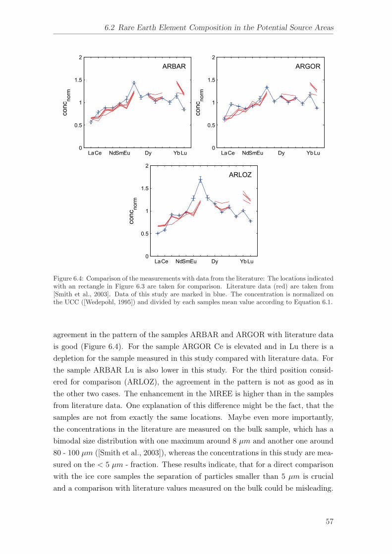
6.2 Rare Earth Element Composition in the Potential Source Areas
LaCe NdSmEu Dy Yb Lu0
0.5
1
1.5
2co
ncno
rmARBAR
LaCe NdSmEu Dy Yb Lu0
0.5
1
1.5
2
conc
norm
ARGOR
LaCe NdSmEu Dy Yb Lu0
0.5
1
1.5
2
conc
norm
ARLOZ
Figure 6.4: Comparison of the measurements with data from the literature: The locations indicatedwith an rectangle in Figure 6.3 are taken for comparison. Literature data (red) are taken from[Smith et al., 2003]. Data of this study are marked in blue. The concentration is normalized onthe UCC ([Wedepohl, 1995]) and divided by each samples mean value according to Equation 6.1.
agreement in the pattern of the samples ARBAR and ARGOR with literature data
is good (Figure 6.4). For the sample ARGOR Ce is elevated and in Lu there is a
depletion for the sample measured in this study compared with literature data. For
the sample ARBAR Lu is also lower in this study. For the third position consid-
ered for comparison (ARLOZ), the agreement in the pattern is not as good as in
the other two cases. The enhancement in the MREE is higher than in the samples
from literature data. One explanation of this difference might be the fact, that the
samples are not from exactly the same locations. Maybe even more importantly,
the concentrations in the literature are measured on the bulk sample, which has a
bimodal size distribution with one maximum around 8 μm and another one around
80 - 100 μm ([Smith et al., 2003]), whereas the concentrations in this study are mea-
sured on the < 5 μm - fraction. These results indicate, that for a direct comparison
with the ice core samples the separation of particles smaller than 5 μm is crucial
and a comparison with literature values measured on the bulk could be misleading.
57

6 Sources of Dust in Dronning Maud Land
LaCe NdSmEu Dy Yb Lu0
0.5
1
1.5
2
2.5
3
conc
norm
(a) Antarctica
LaCe NdSmEu Dy Yb Lu0
0.5
1
1.5
2
2.5
3
conc
norm
(b) Southern Africa
LaCe NdSmEu Dy Yb Lu0
0.5
1
1.5
2
2.5
3
conc
norm
(c) South America
LaCe NdSmEu Dy Yb Lu0
0.5
1
1.5
2
2.5
3
conc
norm
(d) New Zealand (cyan), Australia (blue)
Figure 6.5: REE pattern for different continents. The concentration is normalized on the UCC([Wedepohl, 1995])) and divided by each samples mean value according to Equation 6.1.
Figure 6.5 shows the REE pattern for different continents (concentrations are
normalized according to Equation 6.1).
Some characteristics of the REE pattern in the PSA can already be seen in these
graphs: The samples from Antarctica generally show a decrease from LREE to
HREE ( LREEHREE
= 1.7) and a variable enhancement of the Eu-concentration. The
samples from southern Africa have also higher concentrations of LREE compared to
HREE ( LREEHREE
= 1.4), but much more pronounced is the elevated concentrations in
the MREE. The highest Eu anomaly are found in the samples from New Zealand,
in combination with an elevated HREE concentration compared to LREE ( LREEHREE
= 0.6). Most of the samples are from South America. They all show a slightly
increased concentration of MREE and a small enrichment of HREE compared to
LREE ( LREEHREE
= 0.9).
To get a more quantitative view about these differences and to test wether these
differences are sufficient to provide separation of different PSAs Figure 6.6 shows
the Eu-anomaly Eu∗Eu
versus the ratio LREEHREE
calculated as
58

6.2 Rare Earth Element Composition in the Potential Source Areas
0 0.5 1 1.5 2 2.50
0.5
1
1.5
2
2.5
LRE
E/H
RE
E
Eu*/Eu
Figure 6.6: Comparison of Eu∗Eu vs. LREE
HREE of the different source regions. New Zealand (cyanstars), Antarctica (red diamonds), Australia (blue triangles), South America (green rectangles),southern Africa (black circles). Calculation of Eu∗
Eu and LREEHREE see text. The REE concentration
are normalized on the UCC ([Wedepohl, 1995].
Eu∗
Eu=
√SmUCC · GdUCC
EuUCC
(6.2)
andLREE
HREE=
LaUCC + CeUCC + PrUCC + NdUCC
ErUCC + TmUCC + Y bUCC + LuUCC
(6.3)
with REEUCC the respective element concentration normalized on the concentra-
tion in the UCC ([Wedepohl, 1995]). The features already identified in Figure 6.5
are also clearly apparent in Figure 6.6. Australia can be separated from Antarctica
by different values for LREEHREE
. Furthermore the overlap between the New Zealand
and the Antarctic field is small as well as the South African and the Australian
field. The South American field, which was identified as the main source for dust in
the EPICA-Dome C and Vostok ice core based on Sr/Nd isotopes ([Delmonte et al.,
2002a]), overlaps with all other fields. Whether the areas are sufficiently separated
to identify sources of dust in Antarctic ice cores will be discussed in Section 6.3.
In any case, this approach does not use the full REE fingerprint. In particular the
Eu-anomaly Eu∗Eu
depends only on the three elements Sm, Eu and Gd. Even if the
major variability is expected in Eu and in the ratios between LREE, MREE and
HREE, using the full REE fingerprint could deliver additional information.
59

6 Sources of Dust in Dronning Maud Land
La Ce NdSmEu Dy Yb Lu
−0.4
−0.2
0
0.2
0.4
(a) Principle Component 1
La Ce NdSmEu Dy Yb Lu
−0.6
−0.4
−0.2
0
0.2
0.4
0.6
(b) Principle Component 2
La Ce NdSmEu Dy Yb Lu−0.8
−0.6
−0.4
−0.2
0
0.2
0.4
0.6
0.8
(c) Principle Component 3
La Ce NdSmEu Dy Yb Lu−0.8
−0.6
−0.4
−0.2
0
0.2
0.4
0.6
0.8
(d) Principle Component 4
Figure 6.7: The principal components PC1 to PC4 of the PCA performed on the REE pattern ofthe samples from the PSA. PC1 to PC3 explain 88 %of the total variance.
To use the complete REE spectrum a principal component analysis (PCA) was
performed. The REE span a 14-dimensional space, where each REE spans one
dimension. The REE fingerprint of each sample represents a vector in this 14-
dimensional space with the base (coordinate system) of the REE concentrations
(CSREE). With the principal components (PCs) a new coordinate system with a new
base was established. The PSA samples were transformed from the old coordinate
system CSREE to the new coordinate system spanned by the principal components
(CSPC).
In order not to overweight one continent within the PCA analysis, the number
of samples incorporated in the PCA should be equal and five samples were taken
from each continent. Therefore, the samples from the continents with more than
five samples (South America and Antarctica) were averaged into five groups, where
samples with similar REE pattern were grouped. For continents with less than five
samples available (New Zealand and Australia), literature data were used to fill the
missing positions in the PCA.
60

6.2 Rare Earth Element Composition in the Potential Source Areas
1 2 3 4 5 6 7 8 9 10 11 12 13 140
0.1
0.2
0.3
0.4
0.5
0.6
rela
tive
stre
ngth
of E
igen
valu
es
Number of Eigenvalue
Figure 6.8: Eigenvalue spectrum of the PCA of the PSA. PC1 to PC3 explain 88 % of the totalvariance.
The PCA generated the eigenfunction matrix F and the principal components
PC1 to PC14 (PC1 - PC4 are shown in Figure 6.7). The detailed mathematic
description is given in Appendix E.
The main features of the REE fingerprint as seen in Figure 6.5 are apparent.
PC1 explains the differences between LREE, MREE and HREE. By this principal
component 53 % of the variance is explained. PC2 shows the enrichment in MREE
and explains 24 % of the variance. PC3 shows a very strong peak in Eu and explains
11 % of the variance. PC2 and PC3 show also little variance in Ce. All together
PC1 to PC3 explain 88 % of the total variance. PC4 to PC14 do not show a signal
that obeys any obvious geochemical explanation and account all together only for
12 % of the total variance (Figure 6.8). Therefore, PC4 to PC14 are assigned as
noise and will not be considered further in this study.
One difficulty arises in the determination of the error bars of the PCs. To get
a measure for the dependency of the choice of the samples taken for the PCA, the
PCA was repeated 50 times in the following way: The PCA was performed with 5
samples taken randomly out of the 14 samples of South America. From the other
continents the samples were taken as described before. This was repeated 50 times.
The 50 different PC1 to PC3 obtained in this way are shown in Figure 6.9. In some
cases PC2 and/or PC3 changed their sign (i.e. the direction of the eigenvalue). In
these cases the PC3 is shown in red. Despite this effect the first three PCs do not
show any significant differences, indicating that the selection of the South American
samples for the PCA does not affect the results. In the further work the PC1 to
61

6 Sources of Dust in Dronning Maud Land
La Ce NdSmEu Dy Yb Lu−0.5
0
0.5
(a) Principle Component 1
La Ce NdSmEu Dy Yb Lu
−0.6
−0.4
−0.2
0
0.2
0.4
0.6
(b) Principle Component 2
La Ce NdSmEu Dy Yb Lu−0.8
−0.6
−0.4
−0.2
0
0.2
0.4
0.6
0.8
(c) Principle Component 3
Figure 6.9: The first 3 principal components of the PCA performed on the REE pattern of thesamples from the potential source areas. The PCA was repeated 50 times with 5 randomly chosensamples out of the South America samples each time. In some cases the sign of PC2 and/or PC 3was reversed (see text). These cases are shown in red.
PC3 shown in Figure 6.7 are used.
In a next step all the other samples, which were not taken into account for the
PCA, were transformed into the new coordinate system CSPC according to Equation
6.4
BPC = BREE · F (6.4)
with BPC the coordinates in CSPC , BREE the coordinates in CSREE and the
eigenfunction matrix F (see also Appendix E). Literature data were also included:
77 from South America ([Gaiero et al., 2004]), eleven from New Zealand and five
from Australia ([Marx et al., 2005a]). Since they cover a larger size spectrum than
the Antarctic ice core dust, the data from literature have to be interpretated with
caution. In the PCA-analysis only samples with the full REE-pattern could be
62
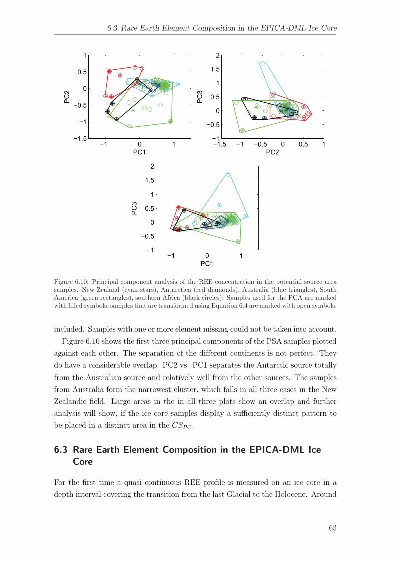
6.3 Rare Earth Element Composition in the EPICA-DML Ice Core
−1 0 1−1.5
−1
−0.5
0
0.5
1
PC1
PC
2
−1.5 −1 −0.5 0 0.5 1−1
−0.5
0
0.5
1
1.5
2
PC2
PC
3
−1 0 1−1
−0.5
0
0.5
1
1.5
2
PC1
PC
3
Figure 6.10: Principal component analysis of the REE concentration in the potential source areasamples. New Zealand (cyan stars), Antarctica (red diamonds), Australia (blue triangles), SouthAmerica (green rectangles), southern Africa (black circles). Samples used for the PCA are markedwith filled symbols, samples that are transformed using Equation 6.4 are marked with open symbols.
included. Samples with one or more element missing could not be taken into account.
Figure 6.10 shows the first three principal components of the PSA samples plotted
against each other. The separation of the different continents is not perfect. They
do have a considerable overlap. PC2 vs. PC1 separates the Antarctic source totally
from the Australian source and relatively well from the other sources. The samples
from Australia form the narrowest cluster, which falls in all three cases in the New
Zealandic field. Large areas in the in all three plots show an overlap and further
analysis will show, if the ice core samples display a sufficiently distinct pattern to
be placed in a distinct area in the CSPC .
6.3 Rare Earth Element Composition in the EPICA-DML IceCore
For the first time a quasi continuous REE profile is measured on an ice core in a
depth interval covering the transition from the last Glacial to the Holocene. Around
63

6 Sources of Dust in Dronning Maud Land
LaCe NdSmEu Dy Yb Lu0
0.5
1
1.5
2
2.5
3
conc
norm
(a) 493-825 m
LaCe NdSmEu Dy Yb Lu0
0.5
1
1.5
2
2.5
3
conc
norm
(b) 825-1100 m
Figure 6.11: Mean REE pattern from different depth intervals from the EPICA-DML ice core.Mean values of the concentrations are normalized according to Equation 6.1. The errorbars givethe standard deviation from the mean value. Data from the depth intervals 808 - 810 m, 1042 -1043 m and 942 - 945 m are excluded (see text).
350 samples of the EPICA-DML ice core are analyzed for REE and several other
TE (for details see Appendix C). They are taken from a depth interval ranging
from 1100 m to 500 m covering the time span of the transition from the last Glacial
to the Holocene (26500 - 7700 yr BP ([Ruth et al., 2007b])). In Appendix C all
REE fingerprints are plotted. Generally the patterns in samples lower than ca. 825
m are very uniform. In this depth interval in almost all samples the full spectrum
could be evaluated. Above 825 m the patterns become more variable and in several
samples the less abundant elements could not be evaluated, in particular in the
depth interval between 625 m and 725 m where the dust concentration is very low
(Figure 6.14). Variations in the relative concentration and deviations from the flat
pattern occur especially for Ce and Eu, consistent with the geochemical behaviour
of the REE (Section 3). In some samples La and Tm show an enhancement.
Figure 6.11(a) shows the averaged REE spectrum of the depth interval from 493
to 825 m, that corresponds to the Holocene and the ACR. The error bars give the
standard deviation from the mean value. Since for different elements the number of
samples with a concentration below the detection limit is different, the number of
samples for each elements mean value is also different. Least values were available
for the less abundant REE (Eu, Tb, Ho, Tm, Yb, Lu). Aside from Lu, all mean
values are within the standart deviation equal one and neither LREE nor HREE
are clearly enriched. A decreasing trend from Dy to Lu is observable. Eu shows the
largest scatter due to the highly variable enhancement or depletion in Eu.
The samples from lower than 825 m are characterized by a very uniform REE
pattern. Figure 6.11(b) shows the mean REE spectrum of the depth interval from
64
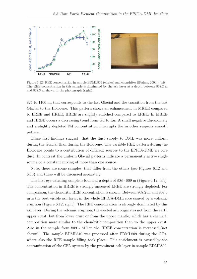
6.3 Rare Earth Element Composition in the EPICA-DML Ice Core
La Ce NdSmEu Dy Yb Lu0
1
2co
nc./C
ont C
rust
, mea
nval
ue
La Ce NdSmEu Dy Yb Lu0
20
40
60
80
100
120
conc
. Cho
ndrit
e/C
ont C
rust
Figure 6.12: REE concentration in sample EDML809 (circles) and chondrites ([Palme, 2004]) (left).The REE concentration in this sample is dominated by the ash layer at a depth between 808.2 mand 808.3 m shown in the photograph (right).
825 to 1100 m, that corresponds to the last Glacial and the transition from the last
Glacial to the Holocene. This pattern shows an enhancement in MREE compared
to LREE and HREE, HREE are slightly enriched compared to LREE. In MREE
and HREE occurs a decreasing trend from Gd to Lu. A small negative Eu-anomaly
and a slightly depleted Nd concentration interrupts the in other respects smooth
pattern.
These first findings suggest, that the dust supply to DML was more uniform
during the Glacial than during the Holocene. The variable REE pattern during the
Holocene points to a contribution of different sources to the EPICA-DML ice core
dust. In contrast the uniform Glacial patterns indicate a permanently active single
source or a constant mixing of more than one source.
Note, there are some samples, that differ from the others (see Figures 6.12 and
6.13) and these will be discussed separately:
The first eye-catching sample is found at a depth of 808 - 809 m (Figure 6.12, left).
The concentration in HREE is strongly increased LREE are strongly depleted. For
comparison, the chondritic REE concentration is shown. Between 808.2 m and 808.3
m is the best visible ash layer, in the whole EPICA-DML core caused by a volcanic
eruption (Figure 6.12, right). The REE concentration is strongly dominated by this
ash layer. During the volcanic eruption, the ejected ash originates not from the earth
upper crust, but from lower crust or from the upper mantle, which has a chemical
composition more similar to the chondritic composition than to the upper crust.
Also in the sample from 809 - 810 m the HREE concentration is increased (not
shown). The sample EDML810 was processed after EDML809 during the CFA,
where also the REE sample filling took place. This enrichment is caused by the
contamination of the CFA-system by the prominent ash layer in sample EDML809.
65

6 Sources of Dust in Dronning Maud Land
La Ce NdSmEu Dy Yb Lu0
1
2
3
4
5
6
conc
./Con
t Cru
st, m
eanv
alue
(a)
La Ce NdSmEu Dy Yb Lu0
0.5
1
1.5
2
2.5
conc
./Con
t Cru
st, m
eanv
alue
(b)
Figure 6.13: Samples, that are deviating from the common REE fingerprint during the glacial:Sample EDML1043 shows an strong enrichment in La and Ce (a). The reason for these enrichmentsis unclear. Sample EDML942 and 944 show an enrichment in LREE (b). For comparison the REEfingerprints of the Antarctic PSA samples are plotted in grey.
Despite intense rinsing of the system the strong REE pattern was carried over in
the samples EDML810.
The next noticeable sample is from a depth of 1042 - 1043 m (Figure 6.13(a)).
This sample shows extremely high values in La and Ce. To exclude an artefact
emerging during the measurement, the samples was remeasured, but showed the
same result. The other chemical species obtained from CFA and IC in this sample
do not show any conspicuities, that would point to any anomaly. Since LREE are
of all REE the most sensitive for contamination, it might also be a possibility, that
this sample was contaminated during filling or during the sample treatment.
There are two other samples in the time interval of the last glacial showing a
noticeable enrichment in LREE. These are from depth 942 - 943 m and 944 - 945
m. The sample from 943 - 944 m was not measured. Therefore it is not clear,
if the pattern is persistent over 3 meters of ice or if it arises from two different
events. The fingerprint of these samples bears resemblance to the fingerprint of
the Antarctic PSA samples (Figure 6.13(b)) indicating that the dust in these two
samples originates from ice free areas on the Antarctic continent. An enrichment in
LREE like in these samples occurs frequently in Holocene samples from the EPICA
Dome C ice core (pers. comm. Paolo Gabrielli), pointing to an Antarctic source for
those samples as well. In contrast to the EPICA Dome C Holocene samples, where
the Antarctic source seems to last for a longer time period, it would be restricted to
the two (or one, if it is persistent over 3 m of ice core) events in the EPICA-DML
ice core during the Glacial.
For the further analysis of dust provenance the above mentioned samples will not
66

6.3 Rare Earth Element Composition in the EPICA-DML Ice Core
500 600 700 800 900 1000 110010−2
10−1
100
101
102
La c
oncn
tratio
n [µ
g m
L−1]
depth [m]500 600 700 800 900 1000 1100
102
103
104
105
106
dust
par
ticle
con
cent
ratio
n [L
−1]
Figure 6.14: Dust (blue line) and La (green line) concentration in the EPICA-DML core in a depthinterval from 493 to 1104 m. The continuous dust profile gives the number concentration measuredusing the LS (unpublished data, Urs Ruth, Patrik Kaufmann). The La is concentration measuredin 1 m bag mean samples. This profile consists of 370 samples taken out of 600.
be taken into account.
In Figure 6.14 the La profile from the EPICA-DML ice core is shown as an example
of the REE in comparison to the dust profile determined with the laser sensor
(personal communication Urs Ruth, Patrik Kaufmann).
REE concentration in ice cores originates from dust in ice cores. The REE con-
centration in seawater is lower than in the crust by 6 orders of magnitude ([Nozaki
et al., 1997]). Therefore marine contributions to the REE concentration in the
samples can be neglected.
The dust concentration during the last Glacial is about two orders of magnitude
higher than during the Holocene. This is consistent with the dust concentration
obtained by CC (Section 5.7) and with other ice cores from Greenland and Antarctica
(e.g. [Fischer et al., 2007a], [Ruth et al., 2003], [EPICA community members, 2006]).
In general the La profile follows closely the dust profile. The La concentration
is about 4 orders of magnitude below the dust number concentration profile, in
accord with the mean La concentration in the UCC. The scatter is higher in the La
concentration, due to the larger error of the measurement.
67
6 Sources of Dust in Dronning Maud Land
6.4 Identification of the DML Dust Provenance
In the following section the REE fingerprints obtained in ice core dust are compared
to those of the PSA samples in order to identify the sources of dust in DML. In a first
step the rations of LREE, MREE and HREE and the Eu∗-anomaly are discussed.
Thereafter, the PCA already presented for the PSA in Section 6.2 is used to refine the
results. In a final step the fingerprints of the South American PSAs are investigated
in more detail.LREEREE
, MREEREE
and HREEREE
are used to exclude or confirm certain continents as a
dust source for DML. Figure 6.15 shows LREEREE
, MREEREE
and HREEREE
and Eu∗Eu
calculated
according to equation 6.2 and 6.3. The black dots give the values in the ice core
samples in the given depth. The colored lines give the upper and lower limit of
the different PSA samples (green: South America, black: Southern Africa, red:
Antarctica, blue: Australia, cyan: New Zealand). Ice core dust lying inside the
range spanned by the colored lines could originate from the source indicated by
the respective color. For samples, with one or more elements below the detection
limit, the values were corrected as follows: In the case one element of the HREE
below the detection limit (e.g. Lu), the remaining sum of HREE (Er + Tm +
Yb) would be approximately 3/4 of the sum of all HREE (Er + Tm + Yb + Lu).
Therefore 1/3 of the remaining sum of HREE (Er + Tm + Yb) was added. For two
elements below the detection limit the remaining sum was doubled and for three
elements below the detection limit tripled. For LREE, MREE and the total sum
of all REE the correction was analogue. For samples with all HREE or MREE
missing, no value is given in the respective plot. For the samples with Sm, Eu or
Gd below the detection limit, no value for Eu∗Eu
is given. The scattering of all values
increase from the Glacial to the Holocene. Some of the Holocene values lie above
the uppermost or below the lowermost line. This is attributed to an overcorrection
of elements below the detection limit. Above 825 m corresponding to 15200 yr BP
([Ruth et al., 2007a]) a lot of samples lie outside the LREEREE
range spanned by the
South American PSA samples indicating that during the warm period dust cannot
be solely from South America. MREEREE
, HREEREE
and Eu∗Eu
do not allow a conclusion of
a dust provenance during the Holocene.
In the following the part below 825 m will be discussed. Considering LREEREE
, the
lower limit for the PSAs in Antarctica is 0.24. There is only one single event out of
166 in the ice core dust with LREEREE
larger than 0.24. Therefore, Antarctica can be
excluded as a major source for DML dust. The PSA samples from Southern Africa
reach a lower limit of LREEREE
= 0.21, that is in the range of the ice core dust (0.18 -
0.24). A non negligible amount of sample have a LREEREE
value below the lower limit of
68

6.4 Identification of the DML Dust Provenance
600 800 10000
0.1
0.2
0.3
0.4
0.5
depth [m]
LRE
E/R
EE
600 800 10000.3
0.4
0.5
0.6
0.7
0.8
depth [m]
MR
EE
/RE
E
600 800 10000.1
0.2
0.3
0.4
0.5
depth [m]
HR
EE
/RE
E
600 800 10000
0.5
1
1.5
2
2.5
3
depth [m]
Eu* /E
u
Figure 6.15: LREEREE , MREE
REE , HREEREE and Eu∗
Eu of the EPICA-DML ice core dust (black dots) and inthe PSA. The colored lines give the upper and lower range of the samples from the respective PSA:New Zealand - cyan, Antarctica - red, Australia - blue, South America - green, Southern Africa -black. Calculation of the ratios are given in the text.
the Southern African PSAs, which therefore can not act as the only source for dust
in DML. The interval covered by MREEREE
in the Australian samples ranges from 0.44
to 0.46, which is well below the ice core dust (MREEREE
= 0.46 - 0.52). Also regardingHREEREE
Australia seems very unlikely as source, since most of the ice core dust values
are below the lower limit of Australia. The mean Eu∗Eu
in the ice core samples is 1.3,
which is in the range of the upper limit of Antarctic dust and just below the upper
limit for New Zealandic dust, excluding Antarctica and New Zealand as the only
sources for the ice core dust.
In summary, analyzing the ratios of LREE, MREE, HREE and the Eu-anomaly,
Antarctica and Australia can be excluded as a source for dust in DML in the time
between 26500 and 15200 yr BP and Southern Africa or New Zealand can be ex-
cluded as the only source. The potential of areas in South America to act as sources
is not confined by these investigations. For the time 15200 to 7500 yr BP no source
is clearly identifiable and the dust input to DML is likely a mixture from different
69

6 Sources of Dust in Dronning Maud Land
500 600 700 800 900 1000 1100102
103
104
105
106
107
depth [m]
dust
con
c. [p
art./
ml]
I II IVIII V VI
Figure 6.16: Dust profile in the EPICA-DML ice core, measured with the CFA laser sensor. Thegrey data represents 1 cm mean values, the colored data represents 1 m mean values and arecolored according to the depth intervals I - VI, that are discussed in the text: mid holocene (I),early Holocene (II), ACR (III), transition (IV), LGM (V), before LGM (VI).
source areas. At least, the dust input to DML cannot originate solely from South
America in contrast to the time between 26500 and 15200 yr BP.
In order to refine these findings, the PCA, already presented for the PSA in
Section 6.2, was applied to the ice core samples.
For the further discussion the profile was divided into six depth intervals, which
will be evaluated separately. In Figure 6.16 these six different depth sections are
marked in different colors and labeled with I to VI.
To identify the provenance of the dust, the REE pattern of the remaining REE pro-
file were transformed into the new coordinate system CSPC as described in Section
6.2. In Figure 6.17 the first two components of the EPICA-DML ice core samples in
the new coordinate system CSPC are plotted separatly in the six intervals defined
in Figure 6.16.
Section I - III: Holocene and Antarctic Cold Reversal (ACR)
In these three sections, covering the time period of the Holocene and the ACR,
the concentration of the most samples are below the detection limit for at least one
element. Those samples, where the full REE fingerprint could be evaluated scatter
widely in the coordinate system CSPC . Some of them do not fall in any of the fields
of the PSA, particularly in the Holocene. This is attributed to the large analytical
70

6.4 Identification of the DML Dust Provenance
uncertainty due to the very low REE concentrations in the Holocene samples.
−1 0 1−1.5
−1
−0.5
0
0.5
1
PC1
PC
2
(a) I: Holocene
−1 0 1−1.5
−1
−0.5
0
0.5
1
PC1
PC
2
(b) II: Early Holocene
−1 0 1−1.5
−1
−0.5
0
0.5
1
PC1
PC
2
(c) III: ACR
−1 0 1−1.5
−1
−0.5
0
0.5
1
PC1
PC
2
(d) IV: Transition
−1 0 1−1.5
−1
−0.5
0
0.5
1
PC1
PC
2
(e) V: LGM
−1 0 1−1.5
−1
−0.5
0
0.5
1
PC1
PC
2
(f) VI: Glacial before LGM
Figure 6.17: EPICA-DML ice core samples in the new coordinate system CSPC : PC2 vs. PC1.EPICA-DML samples from the LGM are marked with red circles, from Glacial times before theLGM with black dots. The continents are marked with fields in different colors: New Zealand -cyan, Antarctica - red, Australia - blue, South America - green, Southern Africa - black.
Section IV: Transition
For section IV, corresponding to the transition from the Glacial to the Holocene,
for more than half of the samples the full REE spectrum could be evaluated. Most
71
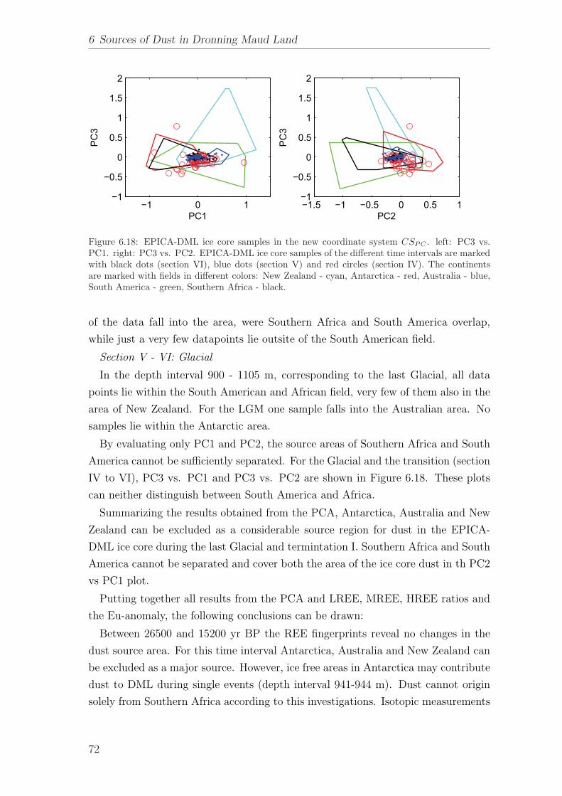
6 Sources of Dust in Dronning Maud Land
−1 0 1−1
−0.5
0
0.5
1
1.5
2
PC1
PC
3
−1.5 −1 −0.5 0 0.5 1−1
−0.5
0
0.5
1
1.5
2
PC2
PC
3
Figure 6.18: EPICA-DML ice core samples in the new coordinate system CSPC . left: PC3 vs.PC1. right: PC3 vs. PC2. EPICA-DML ice core samples of the different time intervals are markedwith black dots (section VI), blue dots (section V) and red circles (section IV). The continentsare marked with fields in different colors: New Zealand - cyan, Antarctica - red, Australia - blue,South America - green, Southern Africa - black.
of the data fall into the area, were Southern Africa and South America overlap,
while just a very few datapoints lie outsite of the South American field.
Section V - VI: Glacial
In the depth interval 900 - 1105 m, corresponding to the last Glacial, all data
points lie within the South American and African field, very few of them also in the
area of New Zealand. For the LGM one sample falls into the Australian area. No
samples lie within the Antarctic area.
By evaluating only PC1 and PC2, the source areas of Southern Africa and South
America cannot be sufficiently separated. For the Glacial and the transition (section
IV to VI), PC3 vs. PC1 and PC3 vs. PC2 are shown in Figure 6.18. These plots
can neither distinguish between South America and Africa.
Summarizing the results obtained from the PCA, Antarctica, Australia and New
Zealand can be excluded as a considerable source region for dust in the EPICA-
DML ice core during the last Glacial and termintation I. Southern Africa and South
America cannot be separated and cover both the area of the ice core dust in th PC2
vs PC1 plot.
Putting together all results from the PCA and LREE, MREE, HREE ratios and
the Eu-anomaly, the following conclusions can be drawn:
Between 26500 and 15200 yr BP the REE fingerprints reveal no changes in the
dust source area. For this time interval Antarctica, Australia and New Zealand can
be excluded as a major source. However, ice free areas in Antarctica may contribute
dust to DML during single events (depth interval 941-944 m). Dust cannot origin
solely from Southern Africa according to this investigations. Isotopic measurements
72

6.4 Identification of the DML Dust Provenance
on Sr and Nd exclude Southern Africa as a source of dust in the EPICA-Dome C and
Vostok ice cores (Figure 6.20 taken from [Delmonte et al., 2004a]), suggesting that
for DML Southern Africa might also account for a minor contribution of the dust
input. Therewith the results of this work point to South America as the provanance
of dust in the EPICA-DML ice core.
Between 15200 and 7500 yr BP the source cannot be identified. However, the
source must have changed, since the LREEREE
-ratio of a lot of ice core dust samples
in this time do not fit into the range spanned by the samples from South America.
The dust concentration between 15200 and 7500 yr BP is very low with a minimum
around 14000 yr BP (680 m). The PCA requires the full REE spectrum. As this is
not given for a lot of samples from this time interval a larger sample volume would
help to obtain full REE spectra even for samples with very low dust concentrations.
A full REE fingerprint could be evaluated in almost all samples below 825 m, where
the dust concentration is about 20 fold higher than in the minumum at 680 m. Less
than 10 mL of sample were used in this study. An increase in sample volume by a
factor of 20 is expected to deliver full REE spectra even for Holocene samples.
Recapitulatory, the REE fingerprint in combination with a PCA is a promising
tool for the evaluation of REE fingerprints. The amount of samples from the PSA
has to be increased to allow a more representative picture, especially for the Southern
Africa region. The ice core samples volume has to be increased for the Holocene
samples. A necessary volume of 200 mL would be still far below the volume used
for isotopic measurements of Sr and Nd.
In a last stage the samples from South America are investigated in more detail to
refine a South American source between 26500 and 15200 yr BP.
A closer look on the South American samples reveals three differing fingerprints
(Figure 6.19). The samples from the Argentinian Pampas at the northern edge of
Patagonia (shown in blue) are characterized by an enrichment of MREE ( LREEMREE
= 0.4), a light enrichment in HREE ( LREEHREE
= 0.7) and a very small positive Eu-
anomaly (Eu∗Eu
= 1.07). The second group of samples include samples from the central
and southern part of Patagonia (shown in red). They are characterized by a variable
positive Eu-anomaly varying between Eu∗Eu
= 1 and Eu∗Eu
= 2, a stronger enrichment
in MREE ( LREEMREE
= 0.3) and again a slight enrichment in HREE ( LREEHREE
= 0.75).
The third group of samples is from Tierra del Fuego from the southermost tip of
the South America continent (shown in yellow). They show an increasing slope
from LREE to HREE ( LREEMREE
= 0.4, LREE/HREE = 0.5) and a small negative
Eu-anomaly (Eu∗Eu
= 0.9). One sampling site at Bahia Blanca (white dot) has a very
similar fingerprint to the samples from Tierra del Fuego.
73
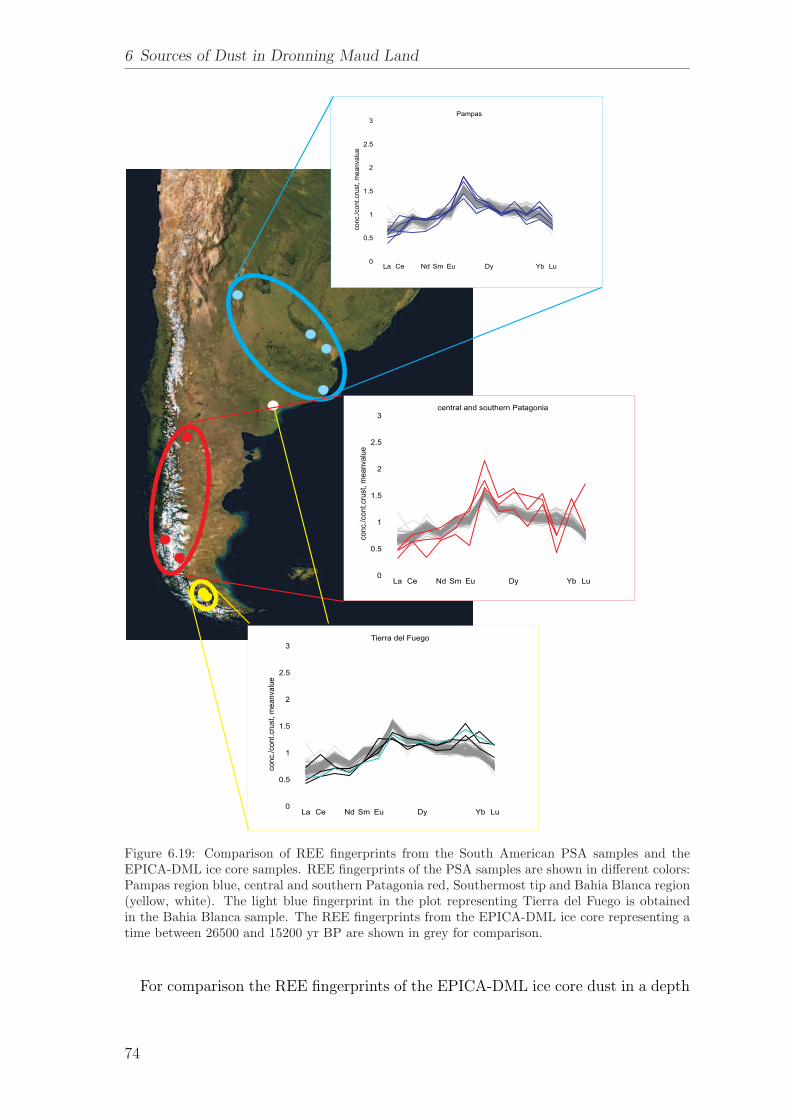
6 Sources of Dust in Dronning Maud Land
La Ce Nd Sm Eu Dy Yb Lu0
0.5
1
1.5
2
2.5
3Tierra del Fuego
conc.
/cont.cr
ust
,m
eanva
lue
La Ce Nd Sm Eu Dy Yb Lu0
0.5
1
1.5
2
2.5
3Pampas
con
c./c
on
t.cr
ust
,m
ea
nva
lue
La Ce Nd Sm Eu Dy Yb Lu0
0.5
1
1.5
2
2.5
3central and southern Patagonia
conc.
/cont.cr
ust
,m
eanva
lue
Figure 6.19: Comparison of REE fingerprints from the South American PSA samples and theEPICA-DML ice core samples. REE fingerprints of the PSA samples are shown in different colors:Pampas region blue, central and southern Patagonia red, Southermost tip and Bahia Blanca region(yellow, white). The light blue fingerprint in the plot representing Tierra del Fuego is obtainedin the Bahia Blanca sample. The REE fingerprints from the EPICA-DML ice core representing atime between 26500 and 15200 yr BP are shown in grey for comparison.
For comparison the REE fingerprints of the EPICA-DML ice core dust in a depth
74

6.4 Identification of the DML Dust Provenance
Figure 6.20: 87Sr/86Sr versus εNd(0). Comparison between ice core dust data from Vostok andEPICA-Dome C and the signature of the < 5 μm fraction of PSA samples (taken from [Delmonteet al., 2004a]).
from 825 to 1100 m are shown. The REE fingerprint of the ice core dust is very
similar to the fingerprint of the samples from the Pampas suggesting that this region
might have acted as a source for Glacial dust for DML. Isotopic measurements on
Sr and Nd reveal the same region as the source for the dust at Dome C and Vostok
during Glacials (Figure 6.20, [Delmonte et al., 2004a]). However, this region is not
considered as a present day dust source ([Prospero et al., 2002]). Therefore, the
distribution of dust sources in South America must have been changed since the last
Glacial.
There are several parameters that may form a strong dust source: Firstly, a large
amount of material available to be outblown, secondly, strong winds and thirdly,
arid climatic conditions. During the last Glacial the Andean glaciers were much
further advanced than today ([Mercer, 1976]), delivering much more clay size ma-
terial. Dryer conditions were observed in Patagonia between 18000 and 14000 yr
BP followed by a moderate increase in precipitation ([Markgraf et al., 2007]). A
significant increase in windspeed could be explained by a more northward position
of the westerly wind belt. At present times the westerly wind belt in the southern
hemisphere is located between 45◦ and 55◦ S. The Pampas region is located at a
latitude of 35◦ S. The results of this work would imply a significant northward shift.
A shift of the Southern Westerlies have been discussed controversial (e.g. [Lamy
et al., 1999], [Heusser, 1990], [Hemming et al., 2007], [Kim et al., 2002], [Wardle,
2003], [Wyrwoll et al., 2000]). The estimates of a possible shift range between up
75

6 Sources of Dust in Dronning Maud Land
to 10◦ northward and a few degree southward. To meet the Pampas region with
the westerly wind belt a northward shift of at least 10◦ would be required, which
is questionable. The amount of samples available from central and southern Patag-
onia is low. A more detailed sampling in this region is essential to scrutinize this
explanation.
As deduced from size distribution measurements the dust concentration changes
between the last Glacial and the ACR in the EPICA-DML ice cores cannot be
explained by transport (Section 5.4 and 5.6), requiring a source change of a factor of
about 28. It is likely that a combination of increased glacial outwash, higher aridity
and an increase of the wind speed in the source area account for this changes. A
more detailed sampling in Patagonia and the Pampas is needed, to investigate, if a
position of the westerly wind belt reaching 35◦S can be confirmed.
76

7 Conclusions and Outlook
The presented work investigates mineral dust in the EPICA-DML ice core. Dust con-
centration and size changes were analyzed in seasonal resolution during the Glacial
and the ACR. The dust provenance was identified for the time between 26500 and
15200 yr BP.
Dust concentrations were found larger during the Glacial than during the ACR
by a factor of 28. On seasonal timescale the dust concentration during the Glacial
varies on average by a factor of 7.6, during the ACR by a factor of 3.5. The mean
dust size spectrum reaching DML during the ACR has a modal value of μ = 1.96
± 0.13 μm and is only slightly, but not significantly larger compared to the mean
size spectrum reaching DML in Glacial times (μ = 1.88 ±0.15 μm ). The seasonal
variability in the size is significantly larger. Typical seasonal changes of μ are 0.2 -
0.3 μm during the Glacial and 0.2 - 0.35 μm during the ACR.
A conceptual model ([Ruth et al., 2003], [Fischer et al., 2007b]) using the changes
in dust size to calculate changes in the effective transport time is applied to the
different time slices. According to this model, the mean effective transport time
does not significantly change between the Glacial and the ACR. In contrary on a
seasonal scale, changes in the effective transport time by a factor of 0.6 during the
Glacial and 0.4 during the ACR are observed.
By knowing the variation in effective transport time, a quantification of transport
and source contributions to the dust concentration changes in the ice core can be
calculated. According to this simple model, the observed dust concentration changes
from the Glacial to the ACR cannot be explained by transport and must therefore
be explained by changes in the source. In contrast on a seasonal scale, during the
ACR between 70 % and 100 % of the seasonal dust variations can be explained by
transport, implying a rather constant source strength throughout the year during
that time. During the Glacial the dust concentration changes arising from trans-
port changes are in the same range, but explain only 30 - 63 % of the higher dust
concentration variations found in the EPICA-DML ice core. Thus, an additional
contribution from the source is necessary to explain the remaining 37 - 70 %.
These results are based on size distribution measurements in two core section of
1 m each. To confirm these findings, equal investigations have to be performed in
other depth intervals. During Interglacials with low dust concentrations a larger
77

7 Conclusions and Outlook
sample volume is needed to obtain better statistics and a continuous profile of the
mode μ. In order not to loose the 3 mm resolution, a larger cross section than 32 · 32
mm from the CFA-cut (Figure 4.2) is needed. Additionally, the same investigations
have to be performed on ice cores from different drill sites.
The use of REE is a promising tool to identify dust provenances. In the EPICA-
DML ice core in a depth interval from 493 to 1105 m REE concentrations are
measured using ICP-SF-MS. Less than 10 mL sample volume was used. For samples
with low dust concentrations not the full REE spectrum could be obtained, as
especially the less abundant elements are below the detection limit.
To identify the dust provenance by use of the REE, 33 samples from the PSA are
analyzed and compared to the ice core samples. Considering the relative enrichment
and depletion of LREE, MREE and HREE Antarctica and Australia could be ex-
cluded as a source before 15200 yr BP. If Southern Africa acts as a source, it cannot
be the only one. By applying a PCA, New Zealand could be excluded as a major
source. The results suggest South America as the major dust source before 15200
yr BP, whereas after 15200 yr BP a mixture of different sources seems more likely.
At least one other source region is needed besides South America to explain the
observed fingerprints. A direct comparison of the REE fingerprints indicates that
the Glacial dust source for DML before 15200 yr BP is located in the Argentinean
Pampas, which could be explained by a significant northward shift of the southern
westerly wind belt during the last Glacial. Indeed, this implication is rather pre-
liminary, since the number of samples from the PSAs used in the presented study
is very limited. More samples are needed to get a clearer picture, especially from
southern Africa and from South America. To investigate the source areas during
warm stages a larger volume of ice core samples of up to 200 g is needed. Therewith
a reduction in samples volume for provenance analysis using REE instead of isotopic
measurements of Sr and Nd by a factor of ≈10 would be reached. REE fingerprints
have shown their potential to serve as a tool for provenance analysis of dust in ice
cores.
78

Appendix


A Preparation of the Samples from the PotentialSource Areas
The samples from the potential source areas were digested according to the scheme
given in the following Table.
sample volume 2 or 5 mLaddition of 10 mL HNO3, 5 mL HF, 5 mL H2O2
digestion according to the following procedurestep duration [h] temperature [◦C] comment0 201 1 100 heat2 12 100 hold3 end let cool to room temperature
close beakers tightly0 201 1 100 heat2 5 100 hold3 1 120 heat4 2 120 hold5 1 140 heat6 2 140 hold7 1 160 heat8 2 160 hold9 1 180 heat10 2 180 hold11 1 210 heat12 5 210 hold13 1.5 170 cool14 1 160 cool15 1.5 140 cool16 1 140 hold17 1 120 cool18 1 100 cool19 end let cool to room temperature
add 10 mL ultra pure water to reduce Al and CaF0 201 1 100 heat2 4 100 hold3 end let cool to room temperature
81

A Preparation of the Samples from the Potential Source Areas
subboiling to 5 - 10 mL to reduce the acidstep duration [h] temperature [◦C] comment0 20 lower heating plate1 2 160 heat2 1.5 160 hold3 end let cool to room temperature0 20 upper heating plate1 1.33 110 heat2 4 110 hold3 end let cool to room temperaturetransfer sample to 25 mL vial, filling up to 25 mL with 2 % HNO3
Table A.1: Full acid digestion of the PSA samples.
82

B ICPMS Additional Information
B.1 Cleaning of lab ware at AWI
1 week industrial cleaning agent (3 % Mucasol, 97 % ultra pure waterrinsing with ultra pure water
1 week HCl-bath (25 % HCl, 75 % ultra pure water)rinsing with ultra pure water
1 week HNO3-bath (25 % HNO3, 75 % ultra pure water)rinsing with ultra pure water
1 week HNO3-bath (10 % HNO3, 90 % ultra pure water)rinsing with ultra pure waterdrying under clean bench class 100sealing twice into PE-bags for storage
Table B.1: Cleaning procedure for the samples vials used for the ICP-MS analysis
Used reagents:
• ultra pure water: production by coupling a reverse osmosis system with a
Purelab ultra system (Elga, High Wycombe, U.K.) (at AWI), production by
coupling a Milli-Q (Millipore, Bedford, MA) water system with a Purelab
Ultra system (Elga, High Wycombe, U.K.) (at University of Venice)
• industrial cleaning agent: MUCASOL, Fa. Merck
• HCl: HCl suprapur, Fa. Merck
• HNO3: HNO3 p.a. 65 %, Fa. Merck
83

B ICPMS Additional Information
B.2 Blank levels
element La Ce Pr Nd Sm Eu Gdblank level [ng/L] 1.61 2.27 1.48 3.44 0.95 0.56 0.74
element Tb Dy Ho Er Tm Yb Lublank level [ng/L] 0.10 0.56 0.15 0.11 0.01 0.36 0.12
Table B.2: Procedural blanks of the samples from the potential source areas performed with theICP-QP-MS determined by the median of 10 replicates
La Ce Nd Sm Eu Dy Yb Lu0
0.005
0.01
0.015
0.02
0.025
0.03
0.035
0.04
0.045
Bla
nk le
vel [
ppt]
0.2 %0.5 %1.0 %2.0 %5.0 %
Figure B.1: Blank levels of the polypropylene sample vials used for the REE analysis in the EDMLice core samples. The different lines indicate different dilutions of HNO3 in ultra pure water.
84

C EDML-samples analyzed on Rare Earth Elements
In the following REE fingerprints are plotted. Normalization was done according to
Equation 6.1. The absolute value on the y-axis indicates the depth of the sample in
the ice core. For example, the sample EDML800 from a depth of 800 m is plotted
on the y-axis at 800. The relative deviation of the individual REE concentrations
(e.g. La concentration, Ce concentration) from the mean value of 800 gives the
fingerprint. Thereafter the measured concentrations are listed in [ng·L−1].
LaCe NdSmEu Dy YbLu550
555
560
565
570
575
580
585
LaCe NdSmEu Dy YbLu640
645
650
655
660
665
670
675
LaCe NdSmEu Dy YbLu520
525
530
535
540
545
550
555
LaCe NdSmEu Dy YbLu610
615
620
625
630
635
640
645
LaCe NdSmEu Dy YbLu490
495
500
505
510
515
520
525
LaCe NdSmEu Dy YbLu580
585
590
595
600
605
610
615
85

C EDML-samples analyzed on Rare Earth Elements
LaCe NdSmEu Dy YbLu760
765
770
775
780
785
790
795
LaCe NdSmEu Dy YbLu880
885
890
895
900
905
910
915
LaCe NdSmEu Dy YbLu730
735
740
745
750
755
760
765
LaCe NdSmEu Dy YbLu850
855
860
865
870
875
880
885
LaCe NdSmEu Dy YbLu700
705
710
715
720
725
730
735
LaCe NdSmEu Dy YbLu820
825
830
835
840
845
850
855
LaCe NdSmEu Dy YbLu670
675
680
685
690
695
700
705
LaCe NdSmEu Dy YbLu790
795
800
805
810
815
820
825
86

LaCe NdSmEu Dy YbLu1000
1005
1010
1015
1020
1025
1030
1035
LaCe NdSmEu Dy YbLu970
975
980
985
990
995
1000
1005
LaCe NdSmEu Dy YbLu1060
1065
1070
1075
1080
1085
1090
1095
LaCe NdSmEu Dy YbLu940
945
950
955
960
965
970
975
LaCe NdSmEu Dy YbLu1030
1035
1040
1045
1050
1055
1060
1065
LaCe NdSmEu Dy YbLu910
915
920
925
930
935
940
945
LaCe NdSmEu Dy YbLu1090
1095
1100
1105
1110
1115
1120
1125
87
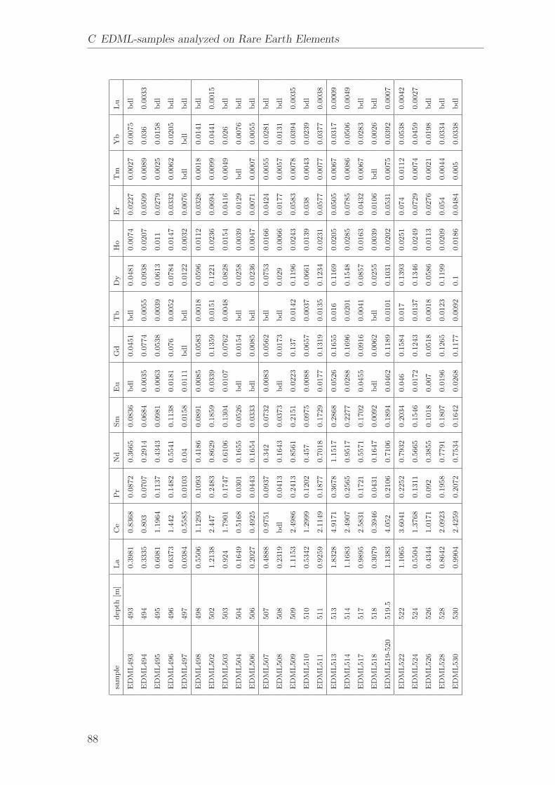
C EDML-samples analyzed on Rare Earth Elements
sam
ple
dep
th[m
]La
Ce
Pr
Nd
Sm
Eu
Gd
Tb
Dy
Ho
Er
Tm
Yb
Lu
ED
ML493
493
0.3
981
0.8
368
0.0
872
0.3
665
0.0
836
bdl
0.0
451
bdl
0.0
481
0.0
074
0.0
227
0.0
027
0.0
075
bdl
ED
ML494
494
0.3
335
0.8
03
0.0
707
0.2
914
0.0
684
0.0
035
0.0
774
0.0
055
0.0
938
0.0
207
0.0
509
0.0
089
0.0
36
0.0
033
ED
ML495
495
0.6
081
1.1
964
0.1
137
0.4
343
0.0
981
0.0
063
0.0
538
0.0
039
0.0
613
0.0
11
0.0
279
0.0
025
0.0
158
bdl
ED
ML496
496
0.6
373
1.4
42
0.1
482
0.5
541
0.1
138
0.0
181
0.0
76
0.0
052
0.0
784
0.0
147
0.0
332
0.0
062
0.0
205
bdl
ED
ML497
497
0.0
384
0.5
585
0.0
103
0.0
40.0
158
0.0
111
bdl
bdl
0.0
122
0.0
032
0.0
076
bdl
bdl
bdl
ED
ML498
498
0.5
506
1.1
293
0.1
093
0.4
186
0.0
891
0.0
085
0.0
583
0.0
018
0.0
596
0.0
112
0.0
328
0.0
018
0.0
141
bdl
ED
ML502
502
1.2
138
2.4
47
0.2
483
0.8
629
0.1
859
0.0
339
0.1
359
0.0
151
0.1
221
0.0
236
0.0
694
0.0
099
0.0
441
0.0
015
ED
ML503
503
0.9
24
1.7
901
0.1
747
0.6
106
0.1
304
0.0
107
0.0
762
0.0
048
0.0
828
0.0
154
0.0
416
0.0
049
0.0
26
bdl
ED
ML504
504
0.1
649
0.5
168
0.0
301
0.1
655
0.0
526
bdl
0.0
154
bdl
0.0
258
0.0
039
0.0
129
bdl
0.0
076
bdl
ED
ML506
506
0.2
027
0.4
925
0.0
443
0.1
654
0.0
333
bdl
0.0
085
bdl
0.0
236
0.0
047
0.0
071
0.0
007
0.0
055
bdl
ED
ML507
507
0.4
888
0.9
751
0.0
937
0.3
42
0.0
732
0.0
083
0.0
562
bdl
0.0
753
0.0
166
0.0
424
0.0
055
0.0
281
bdl
ED
ML508
508
0.2
319
bdl
0.0
413
0.1
643
0.0
373
bdl
0.0
173
bdl
0.0
29
0.0
066
0.0
177
0.0
057
0.0
131
bdl
ED
ML509
509
1.1
153
2.4
986
0.2
413
0.8
561
0.2
151
0.0
223
0.1
37
0.0
142
0.1
196
0.0
243
0.0
583
0.0
078
0.0
394
0.0
035
ED
ML510
510
0.5
342
1.2
999
0.1
202
0.4
57
0.0
975
0.0
088
0.0
657
0.0
037
0.0
661
0.0
139
0.0
38
0.0
043
0.0
239
bdl
ED
ML511
511
0.9
259
2.1
149
0.1
877
0.7
018
0.1
729
0.0
177
0.1
319
0.0
135
0.1
234
0.0
231
0.0
577
0.0
077
0.0
377
0.0
038
ED
ML513
513
1.8
328
4.9
171
0.3
678
1.1
517
0.2
868
0.0
526
0.1
655
0.0
16
0.1
169
0.0
205
0.0
505
0.0
067
0.0
317
0.0
009
ED
ML514
514
1.1
683
2.4
907
0.2
565
0.9
517
0.2
277
0.0
288
0.1
696
0.0
201
0.1
548
0.0
285
0.0
785
0.0
086
0.0
506
0.0
049
ED
ML517
517
0.9
895
2.5
831
0.1
721
0.5
571
0.1
702
0.0
455
0.0
916
0.0
041
0.0
857
0.0
163
0.0
432
0.0
067
0.0
283
bdl
ED
ML518
518
0.3
079
0.3
946
0.0
431
0.1
647
0.0
092
bdl
0.0
062
bdl
0.0
255
0.0
039
0.0
106
bdl
0.0
026
bdl
ED
ML519-5
20
519.5
1.1
383
4.0
52
0.2
106
0.7
106
0.1
894
0.0
462
0.1
189
0.0
101
0.1
031
0.0
202
0.0
531
0.0
075
0.0
392
0.0
007
ED
ML522
522
1.1
065
3.6
041
0.2
252
0.7
932
0.2
034
0.0
46
0.1
584
0.0
17
0.1
393
0.0
251
0.0
74
0.0
112
0.0
538
0.0
042
ED
ML524
524
0.5
504
1.3
768
0.1
311
0.5
665
0.1
546
0.0
172
0.1
243
0.0
137
0.1
346
0.0
249
0.0
729
0.0
074
0.0
459
0.0
027
ED
ML526
526
0.4
344
1.0
171
0.0
92
0.3
855
0.1
018
0.0
07
0.0
518
0.0
018
0.0
586
0.0
113
0.0
276
0.0
021
0.0
198
bdl
ED
ML528
528
0.8
642
2.0
923
0.1
958
0.7
791
0.1
807
0.0
196
0.1
265
0.0
123
0.1
199
0.0
209
0.0
54
0.0
044
0.0
334
bdl
ED
ML530
530
0.9
904
2.4
259
0.2
072
0.7
534
0.1
642
0.0
268
0.1
177
0.0
092
0.1
0.0
186
0.0
484
0.0
05
0.0
338
bdl
88

sam
ple
dep
th[m
]La
Ce
Pr
Nd
Sm
Eu
Gd
Tb
Dy
Ho
Er
Tm
Yb
Lu
ED
ML531
531
0.5
972
1.2
986
0.1
281
0.5
048
0.1
297
0.0
114
0.0
839
0.0
042
0.0
798
0.0
166
0.0
396
0.0
05
0.0
276
bdl
ED
ML532
532
0.6
591
1.5
342
0.1
537
0.6
377
0.1
437
0.0
153
0.0
954
0.0
082
0.0
964
0.0
205
0.0
449
0.0
066
0.0
326
bdl
ED
ML533
533
0.7
764
1.5
723
0.1
634
0.6
099
0.1
597
0.0
315
0.1
08
0.0
148
0.1
041
0.0
218
0.0
512
0.0
069
0.0
36
0.0
026
ED
ML534
534
1.6
575
3.0
75
0.3
737
1.2
858
0.2
784
0.0
582
0.2
489
0.0
337
0.2
024
0.0
44
0.1
224
0.0
226
0.0
911
0.0
126
ED
ML536
536
0.3
199
0.7
037
0.0
68
0.2
785
0.0
596
bdl
0.0
323
bdl
0.0
412
0.0
073
0.0
184
bdl
0.0
154
bdl
ED
ML537
537
1.8
846
2.9
109
0.3
493
1.0
388
0.2
252
0.2
94
0.1
718
0.0
192
0.1
331
0.0
293
0.0
704
0.0
136
0.0
642
0.0
059
ED
ML538
538
0.5
727
1.0
702
0.1
016
0.3
937
0.0
911
bdl
0.0
536
bdl
0.0
577
0.0
099
0.0
338
0.0
021
0.0
199
bdl
ED
ML540
540
0.8
487
1.7
167
0.1
85
0.6
099
0.1
51
0.0
178
0.0
688
0.0
041
0.0
785
0.0
129
0.0
373
0.0
043
0.0
343
bdl
ED
ML541
541
0.1
015
0.1
555
0.0
09
0.0
288
bdl
bdl
bdl
bdl
0.0
133
0.0
023
0.0
063
bdl
bdl
bdl
ED
ML542
542
4.2
564
7.9
885
0.7
526
1.5
774
0.2
58
0.0
524
0.2
337
0.0
278
0.2
128
0.0
458
0.1
236
0.0
174
0.0
972
0.0
125
ED
ML543
543
0.2
038
bdl
0.0
272
0.0
955
0.0
204
0.0
059
bdl
bdl
0.0
208
0.0
076
0.0
187
bdl
bdl
bdl
ED
ML544
544
0.4
342
0.9
947
0.0
934
0.4
047
0.1
079
0.0
193
0.1
037
0.0
09
0.0
994
0.0
196
0.0
534
0.0
063
0.0
401
bdl
ED
ML546
546
0.5
582
1.1
832
0.1
113
0.5
742
0.1
074
0.0
096
0.0
742
0.0
04
0.0
65
0.0
153
0.0
359
0.0
078
0.0
258
0.0
133
ED
ML547
547
0.3
461
bdl
0.0
72
0.3
008
0.0
713
0.0
096
0.0
3bdl
0.0
402
0.0
081
0.0
209
bdl
0.0
066
bdl
ED
ML548
548
0.8
044
2.2
587
0.1
799
0.6
682
0.1
443
0.0
202
0.0
981
0.0
086
0.0
941
0.0
183
0.0
427
0.0
059
0.0
245
bdl
ED
ML549
549
1.2
036
2.1
588
0.2
809
0.8
626
0.2
192
0.1
348
0.1
709
0.0
398
0.1
478
0.0
514
0.0
853
0.0
318
0.0
612
0.0
26
ED
ML550
550
3.5
845
5.6
695
0.7
304
2.5
042
0.5
723
0.1
173
0.5
227
0.0
711
0.4
755
0.0
964
0.2
773
0.0
386
0.2
502
0.0
346
ED
ML551
551
0.0
627
0.1
989
bdl
0.0
686
0.0
457
bdl
bdl
bdl
0.0
122
0.0
046
0.0
048
bdl
bdl
bdl
ED
ML552
552
0.2
033
0.5
074
0.0
466
0.2
131
0.0
598
bdl
0.0
329
bdl
0.0
321
0.0
072
0.0
181
0.0
02
0.0
087
bdl
ED
ML554
554
0.0
738
0.2
648
0.0
089
0.1
046
0.0
368
bdl
0.0
071
bdl
0.0
198
0.0
034
0.0
074
bdl
bdl
bdl
ED
ML556
556
0.7
065
1.0
385
0.1
282
0.4
499
0.0
773
bdl
0.0
33
bdl
0.0
312
0.0
064
0.0
135
0.0
019
0.0
073
bdl
ED
ML557
557
0.3
25
0.7
415
0.0
68
0.2
826
0.0
573
bdl
0.0
304
bdl
0.0
525
0.0
099
0.0
201
0.0
019
0.0
16
bdl
ED
ML558
558
0.4
06
0.8
853
0.0
729
0.3
312
0.0
791
bdl
0.0
327
bdl
0.0
444
0.0
087
0.0
208
0.0
013
0.0
159
bdl
ED
ML559
559
0.2
188
0.5
03
0.0
454
0.2
012
0.0
475
bdl
0.0
278
bdl
0.0
422
0.0
075
0.0
197
0.0
02
0.0
124
bdl
ED
ML560
560
0.5
934
1.3
132
0.1
312
0.5
11
0.1
397
0.0
252
0.0
94
0.0
072
0.0
845
0.0
159
0.0
414
0.0
062
0.0
299
bdl
89

C EDML-samples analyzed on Rare Earth Elements
sam
ple
dep
th[m
]La
Ce
Pr
Nd
Sm
Eu
Gd
Tb
Dy
Ho
Er
Tm
Yb
Lu
ED
ML561
561
0.7
083
1.6
404
0.1
456
0.6
172
0.1
638
0.0
258
0.1
197
0.0
11
0.1
039
0.0
215
0.0
561
0.0
063
0.0
396
0.0
024
ED
ML562
562
0.2
953
0.5
714
0.0
583
0.2
577
0.0
503
bdl
0.0
377
bdl
0.0
42
0.0
095
0.0
238
0.0
035
0.0
127
bdl
ED
ML563
563
0.1
158
0.3
199
0.0
259
0.1
547
0.0
347
0.0
154
0.0
135
bdl
0.0
246
0.0
049
0.0
087
0.0
021
0.0
066
bdl
ED
ML564
564
0.1
719
0.4
122
0.0
367
0.1
797
0.0
385
bdl
0.0
137
bdl
0.0
201
0.0
051
0.0
114
0.0
01
0.0
047
bdl
ED
ML566
566
0.9
411
1.7
118
0.1
793
0.6
443
0.1
683
0.0
259
0.1
226
0.0
196
0.1
228
0.0
302
0.0
693
0.0
151
0.0
524
0.0
114
ED
ML567
567
0.5
613
1.0
531
0.1
082
0.3
868
0.0
484
bdl
0.0
396
bdl
0.0
486
0.0
092
0.0
224
0.0
021
0.0
076
bdl
ED
ML568
568
1.3
305
2.9
216
0.3
637
1.3
673
0.3
109
0.0
448
0.2
296
0.0
27
0.1
757
0.0
314
0.0
762
0.0
11
0.0
486
0.0
01
ED
ML569
569
0.2
279
0.4
735
0.0
503
0.2
034
0.0
434
bdl
0.0
182
bdl
0.0
264
0.0
057
0.0
119
0.0
022
0.0
061
bdl
ED
ML570
570
0.2
609
bdl
0.0
596
0.2
809
0.0
54
0.0
061
0.0
349
bdl
0.0
502
0.0
096
0.0
197
bdl
0.0
13
bdl
ED
ML571
571
1.1
039
3.1
971
0.3
989
1.5
39
0.3
812
0.0
577
0.2
522
0.0
295
0.1
838
0.0
304
0.0
719
0.0
082
0.0
422
0.0
04
ED
ML572
572
0.1
172
0.1
887
0.0
106
0.0
814
bdl
bdl
bdl
bdl
0.0
15
0.0
044
0.0
108
bdl
bdl
bdl
ED
ML574
574
0.5
403
1.5
037
0.1
913
1.0
61
0.4
264
0.0
262
0.4
729
0.0
645
0.4
533
0.0
892
0.2
355
0.0
327
0.1
827
0.0
202
ED
ML576
576
0.2
325
0.5
124
0.0
409
0.1
69
bdl
bdl
0.0
115
bdl
0.0
252
0.0
051
0.0
093
0.0
01
0.0
046
bdl
ED
ML577
577
0.1
753
0.3
678
0.0
278
0.1
487
0.0
311
bdl
0.0
155
bdl
0.0
253
0.0
056
0.0
149
0.0
011
0.0
108
bdl
ED
ML578
578
1.3
215
2.9
071
0.2
785
1.1
021
0.2
636
0.0
354
0.1
991
0.0
239
0.1
723
0.0
328
0.0
814
0.0
097
0.0
596
0.0
044
ED
ML579
579
1.2
578
2.5
213
0.2
671
1.0
02
0.2
46
0.0
721
0.2
018
0.0
236
0.1
654
0.0
315
0.0
828
0.0
10.0
567
0.0
044
ED
ML580
580
0.5
251
1.2
201
0.1
265
0.5
056
0.1
02
0.0
109
0.0
83
0.0
037
0.0
798
0.0
141
0.0
386
0.0
038
0.0
321
bdl
ED
ML581
581
0.9
334
2.0
173
0.2
054
0.8
002
0.1
85
0.0
252
0.1
418
0.0
149
0.1
316
0.0
266
0.0
65
0.0
094
0.0
489
0.0
039
ED
ML582
582
1.2
388
2.2
384
0.2
492
0.8
241
0.2
094
0.0
349
0.1
53
0.0
162
0.1
359
0.0
266
0.0
704
0.0
10.0
547
0.0
032
ED
ML583
583
0.2
11
0.5
622
0.0
553
0.2
415
0.0
522
0.0
031
0.0
333
bdl
0.0
516
0.0
093
0.0
195
0.0
019
0.0
075
bdl
ED
ML584
584
1.3
896
4.0
594
0.3
011
1.0
961
0.2
286
0.0
299
0.1
80.0
193
0.1
514
0.0
265
0.0
752
0.0
11
0.0
531
0.0
012
ED
ML586
586
0.6
456
1.3
52
0.1
767
0.8
205
0.2
374
0.0
099
0.3
031
0.0
466
0.3
30.0
688
0.1
869
0.0
26
0.1
522
0.0
15
ED
ML589
589
8.3
119
10.2
061
1.5
193
4.9
303
1.0
684
0.4
128
0.9
829
0.1
418
0.9
52
0.2
01
0.5
871
0.0
797
0.5
218
0.0
775
ED
ML592
592
0.4
334
0.6
082
0.0
707
0.2
971
0.0
555
0.0
069
0.0
462
bdl
0.0
654
0.0
109
0.0
45
0.0
048
0.0
386
bdl
ED
ML593
593
0.8
807
3.7
983
0.1
676
0.6
157
0.1
51
0.0
449
0.0
938
0.0
07
0.0
722
0.0
178
0.0
409
0.0
059
0.0
264
bdl
90
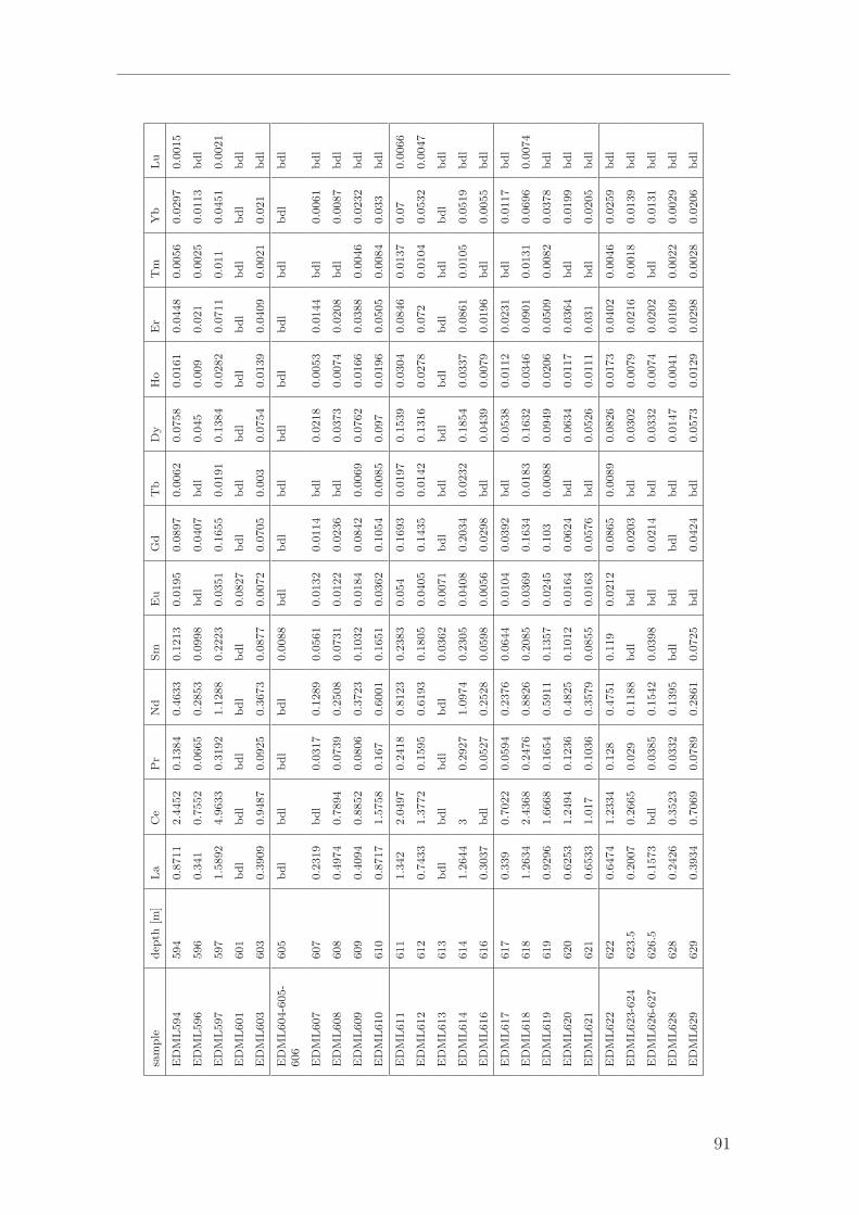
sam
ple
dep
th[m
]La
Ce
Pr
Nd
Sm
Eu
Gd
Tb
Dy
Ho
Er
Tm
Yb
Lu
ED
ML594
594
0.8
711
2.4
452
0.1
384
0.4
633
0.1
213
0.0
195
0.0
897
0.0
062
0.0
758
0.0
161
0.0
448
0.0
056
0.0
297
0.0
015
ED
ML596
596
0.3
41
0.7
552
0.0
665
0.2
853
0.0
998
bdl
0.0
407
bdl
0.0
45
0.0
09
0.0
21
0.0
025
0.0
113
bdl
ED
ML597
597
1.5
892
4.9
633
0.3
192
1.1
288
0.2
223
0.0
351
0.1
655
0.0
191
0.1
384
0.0
282
0.0
711
0.0
11
0.0
451
0.0
021
ED
ML601
601
bdl
bdl
bdl
bdl
bdl
0.0
827
bdl
bdl
bdl
bdl
bdl
bdl
bdl
bdl
ED
ML603
603
0.3
909
0.9
487
0.0
925
0.3
673
0.0
877
0.0
072
0.0
705
0.0
03
0.0
754
0.0
139
0.0
409
0.0
021
0.0
21
bdl
ED
ML604-6
05-
606
605
bdl
bdl
bdl
bdl
0.0
088
bdl
bdl
bdl
bdl
bdl
bdl
bdl
bdl
bdl
ED
ML607
607
0.2
319
bdl
0.0
317
0.1
289
0.0
561
0.0
132
0.0
114
bdl
0.0
218
0.0
053
0.0
144
bdl
0.0
061
bdl
ED
ML608
608
0.4
974
0.7
894
0.0
739
0.2
508
0.0
731
0.0
122
0.0
236
bdl
0.0
373
0.0
074
0.0
208
bdl
0.0
087
bdl
ED
ML609
609
0.4
094
0.8
852
0.0
806
0.3
723
0.1
032
0.0
184
0.0
842
0.0
069
0.0
762
0.0
166
0.0
388
0.0
046
0.0
232
bdl
ED
ML610
610
0.8
717
1.5
758
0.1
67
0.6
001
0.1
651
0.0
362
0.1
054
0.0
085
0.0
97
0.0
196
0.0
505
0.0
084
0.0
33
bdl
ED
ML611
611
1.3
42
2.0
497
0.2
418
0.8
123
0.2
383
0.0
54
0.1
693
0.0
197
0.1
539
0.0
304
0.0
846
0.0
137
0.0
70.0
066
ED
ML612
612
0.7
433
1.3
772
0.1
595
0.6
193
0.1
805
0.0
405
0.1
435
0.0
142
0.1
316
0.0
278
0.0
72
0.0
104
0.0
532
0.0
047
ED
ML613
613
bdl
bdl
bdl
bdl
0.0
362
0.0
071
bdl
bdl
bdl
bdl
bdl
bdl
bdl
bdl
ED
ML614
614
1.2
644
30.2
927
1.0
974
0.2
305
0.0
408
0.2
034
0.0
232
0.1
854
0.0
337
0.0
861
0.0
105
0.0
519
bdl
ED
ML616
616
0.3
037
bdl
0.0
527
0.2
528
0.0
598
0.0
056
0.0
298
bdl
0.0
439
0.0
079
0.0
196
bdl
0.0
055
bdl
ED
ML617
617
0.3
39
0.7
022
0.0
594
0.2
376
0.0
644
0.0
104
0.0
392
bdl
0.0
538
0.0
112
0.0
231
bdl
0.0
117
bdl
ED
ML618
618
1.2
634
2.4
368
0.2
476
0.8
826
0.2
085
0.0
369
0.1
634
0.0
183
0.1
632
0.0
346
0.0
901
0.0
131
0.0
696
0.0
074
ED
ML619
619
0.9
296
1.6
668
0.1
654
0.5
911
0.1
357
0.0
245
0.1
03
0.0
088
0.0
949
0.0
206
0.0
509
0.0
082
0.0
378
bdl
ED
ML620
620
0.6
253
1.2
494
0.1
236
0.4
825
0.1
012
0.0
164
0.0
624
bdl
0.0
634
0.0
117
0.0
364
bdl
0.0
199
bdl
ED
ML621
621
0.6
533
1.0
17
0.1
036
0.3
579
0.0
855
0.0
163
0.0
576
bdl
0.0
526
0.0
111
0.0
31
bdl
0.0
205
bdl
ED
ML622
622
0.6
474
1.2
334
0.1
28
0.4
751
0.1
19
0.0
212
0.0
865
0.0
089
0.0
826
0.0
173
0.0
402
0.0
046
0.0
259
bdl
ED
ML623-6
24
623.5
0.2
007
0.2
665
0.0
29
0.1
188
bdl
bdl
0.0
203
bdl
0.0
302
0.0
079
0.0
216
0.0
018
0.0
139
bdl
ED
ML626-6
27
626.5
0.1
573
bdl
0.0
385
0.1
542
0.0
398
bdl
0.0
214
bdl
0.0
332
0.0
074
0.0
202
bdl
0.0
131
bdl
ED
ML628
628
0.2
426
0.3
523
0.0
332
0.1
395
bdl
bdl
bdl
bdl
0.0
147
0.0
041
0.0
109
0.0
022
0.0
029
bdl
ED
ML629
629
0.3
934
0.7
069
0.0
789
0.2
861
0.0
725
bdl
0.0
424
bdl
0.0
573
0.0
129
0.0
298
0.0
028
0.0
206
bdl
91

C EDML-samples analyzed on Rare Earth Elements
sam
ple
dep
th[m
]La
Ce
Pr
Nd
Sm
Eu
Gd
Tb
Dy
Ho
Er
Tm
Yb
Lu
ED
ML630
630
0.5
807
1.2
858
0.1
468
0.5
25
0.1
008
bdl
0.0
376
bdl
0.0
308
0.0
04
0.0
093
bdl
bdl
bdl
ED
ML632
632
3.8
35
4.1
059
0.6
597
2.2
278
0.4
046
0.0
994
0.4
008
0.0
545
0.4
177
0.0
916
0.2
574
0.0
364
0.2
367
0.0
269
ED
ML633
633
0.0
392
0.1
054
bdl
0.0
385
bdl
bdl
bdl
bdl
bdl
bdl
bdl
bdl
bdl
bdl
ED
ML634
634
0.1
007
0.3
363
0.0
151
0.0
601
0.0
107
bdl
bdl
bdl
0.0
15
0.0
034
0.0
037
bdl
bdl
bdl
ED
ML637
637
bdl
bdl
bdl
bdl
bdl
bdl
bdl
bdl
bdl
bdl
bdl
bdl
bdl
bdl
ED
ML638
638
4.7
081
5.1
896
0.7
768
2.5
861
0.5
494
0.0
907
0.5
307
0.0
665
0.4
684
0.0
986
0.2
701
0.0
367
0.2
297
0.0
269
ED
ML639
639
0.5
306
1.2
412
0.1
242
0.4
199
0.0
72
bdl
0.0
506
bdl
0.0
507
0.0
099
0.0
245
0.0
025
0.0
113
bdl
ED
ML640
640
0.3
733
0.7
721
0.0
739
0.2
711
0.0
561
bdl
0.0
388
bdl
0.0
373
0.0
067
0.0
189
0.0
026
0.0
107
bdl
ED
ML641
641
0.1
383
bdl
0.0
224
0.1
152
0.0
238
bdl
bdl
bdl
0.0
141
bdl
0.0
051
bdl
bdl
bdl
ED
ML642
642
0.2
041
0.4
43
0.0
38
0.1
577
0.0
39
0.0
042
0.0
163
bdl
0.0
272
0.0
067
0.0
151
0.0
019
0.0
046
bdl
ED
ML647
647
0.3
491
0.3
389
0.0
351
0.1
308
0.0
17
bdl
bdl
bdl
0.0
22
0.0
042
0.0
067
bdl
0.0
131
bdl
ED
ML650
650
0.1
535
0.4
346
0.0
328
0.1
681
0.0
479
bdl
0.0
274
bdl
0.0
492
0.0
085
0.0
20.0
037
0.0
097
bdl
ED
ML651
651
0.2
484
0.6
45
0.0
739
0.3
489
0.0
95
0.0
131
0.0
922
0.0
082
0.1
012
0.0
203
0.0
582
0.0
081
0.0
412
bdl
ED
ML653
653
3.0
055
3.2
832
0.4
919
2.7
23
0.2
793
0.0
599
0.2
634
0.0
363
0.2
994
0.0
563
0.1
608
0.0
234
0.1
339
0.0
202
ED
ML654
654
0.2
015
0.5
121
0.0
425
0.1
61
0.0
196
0.0
327
0.0
204
bdl
0.0
226
0.0
037
0.0
125
0.0
01
0.0
061
bdl
ED
ML658
658
0.5
434
1.2
02
0.1
192
0.4
055
0.0
543
bdl
bdl
bdl
bdl
bdl
bdl
bdl
bdl
bdl
ED
ML659
659
0.3
828
0.9
182
0.0
887
0.3
741
0.0
84
0.0
073
0.0
509
0.0
014
0.0
51
0.0
109
0.0
228
0.0
035
0.0
139
bdl
ED
ML660
660
0.1
855
0.4
047
0.0
48
0.2
573
0.0
624
bdl
0.0
448
bdl
0.0
415
0.0
087
0.0
211
0.0
026
0.0
076
bdl
ED
ML661
661
0.2
479
0.5
09
0.0
449
0.1
986
0.0
435
bdl
0.0
133
bdl
0.0
294
0.0
047
0.0
107
0.0
012
0.0
032
bdl
ED
ML662
662
0.3
017
0.7
111
0.0
598
0.2
935
0.0
422
0.0
051
0.0
273
bdl
0.0
294
0.0
069
0.0
192
bdl
0.0
054
bdl
ED
ML663
663
0.4
712
1.0
653
0.1
07
0.4
205
0.0
877
0.0
086
0.0
623
bdl
0.0
636
0.0
129
0.0
274
bdl
0.0
142
bdl
ED
ML664
664
0.4
614
0.8
377
0.0
871
0.2
993
0.0
499
bdl
0.0
33
bdl
0.0
375
0.0
072
0.0
175
0.0
018
0.0
093
bdl
ED
ML666
666
0.0
192
bdl
bdl
bdl
bdl
bdl
bdl
bdl
bdl
bdl
bdl
bdl
bdl
bdl
ED
ML667
667
bdl
bdl
bdl
bdl
bdl
bdl
bdl
bdl
bdl
bdl
bdl
bdl
bdl
bdl
ED
ML668
668
0.0
885
0.2
592
0.0
191
0.1
112
bdl
bdl
bdl
bdl
0.0
18
0.0
049
0.0
095
bdl
0.0
056
bdl
92

sam
ple
dep
th[m
]La
Ce
Pr
Nd
Sm
Eu
Gd
Tb
Dy
Ho
Er
Tm
Yb
Lu
ED
ML669
669
0.8
179
0.8
534
0.1
193
0.4
062
0.1
048
0.0
223
0.0
573
bdl
0.0
632
0.0
138
0.0
368
0.0
062
0.0
25
bdl
ED
ML670
670
0.2
357
0.6
659
0.0
571
0.2
39
0.0
537
0.0
05
0.0
207
bdl
0.0
289
0.0
061
0.0
151
0.0
014
0.0
018
bdl
ED
ML671
671
0.0
748
0.0
612
0.0
052
0.0
318
bdl
bdl
bdl
bdl
bdl
bdl
bdl
bdl
bdl
bdl
ED
ML673
673
bdl
bdl
bdl
bdl
bdl
bdl
bdl
bdl
bdl
bdl
bdl
bdl
bdl
bdl
ED
ML674
674
0.1
939
1.3
121
0.0
344
0.1
613
0.0
361
bdl
0.0
09
bdl
0.0
231
0.0
046
0.0
109
0.0
017
bdl
bdl
ED
ML676
676
bdl
bdl
bdl
bdl
bdl
bdl
bdl
bdl
bdl
bdl
bdl
bdl
bdl
bdl
ED
ML677
677
0.3
391
0.7
687
0.0
684
0.2
557
0.0
635
0.0
089
0.0
452
bdl
0.0
481
0.0
091
0.0
242
0.0
026
0.0
11
bdl
ED
ML678
678
0.0
405
0.1
398
0.0
087
0.0
879
bdl
0.0
239
bdl
bdl
0.0
132
0.0
025
0.0
033
bdl
0.0
037
bdl
ED
ML679
679
0.3
235
0.6
209
0.0
569
0.2
362
0.0
478
bdl
0.0
207
bdl
0.0
26
0.0
062
0.0
144
bdl
0.0
117
bdl
ED
ML680
680
0.3
188
0.9
976
0.0
195
0.0
344
bdl
bdl
bdl
bdl
bdl
bdl
bdl
bdl
bdl
bdl
ED
ML681
681
1.1
793
2.9
181
0.1
963
0.6
478
0.2
128
0.0
445
0.1
17
0.0
095
0.1
103
0.0
245
0.0
627
0.0
097
0.0
492
0.0
03
ED
ML682
682
0.2
91.1
996
0.0
413
0.1
897
0.0
519
bdl
0.0
205
bdl
0.0
279
0.0
07
0.0
163
0.0
015
0.0
062
bdl
ED
ML683
683
0.2
017
0.5
492
0.0
03
bdl
0.0
59
0.0
179
bdl
bdl
bdl
bdl
bdl
bdl
bdl
bdl
ED
ML684
684
0.1
314
0.2
529
0.0
148
0.0
794
0.0
205
bdl
bdl
bdl
0.0
091
0.0
018
0.0
024
bdl
bdl
bdl
ED
ML686
686
0.3
981
0.9
878
0.0
40.1
126
0.0
818
0.0
29
0.0
07
bdl
0.0
205
0.0
071
0.0
189
0.0
037
0.0
064
bdl
ED
ML687
687
1.8
563
3.6
427
0.3
105
1.0
038
0.2
561
0.0
683
0.2
084
0.0
246
0.2
024
0.0
449
0.1
298
0.0
186
0.1
10.0
138
ED
ML688
688
1.4
965
1.7
038
0.2
811
0.9
925
0.2
001
0.0
412
0.1
73
0.0
20.1
893
0.0
393
0.1
225
0.0
168
0.1
035
0.0
105
ED
ML689
689
1.0
415
0.8
785
0.1
242
0.3
583
0.0
528
0.0
32
0.0
345
bdl
0.0
484
0.0
109
0.0
28
0.0
036
0.0
214
bdl
ED
ML691
691
5.5
255
6.5
955
1.0
119
3.3
662
0.7
303
0.1
625
0.6
906
0.0
955
0.6
587
0.1
464
0.4
208
0.0
606
0.3
808
0.0
558
ED
ML693
693
2.1
744
6.0
781
0.3
595
1.1
415
0.2
839
0.0
574
0.2
08
0.0
238
0.1
936
0.0
407
0.1
111
0.0
182
0.0
881
0.0
083
ED
ML694
694
1.2
48
3.3
864
0.2
341
0.7
612
0.1
841
0.0
463
0.0
93
0.0
056
0.0
805
0.0
149
0.0
387
0.0
066
0.0
213
bdl
ED
ML696
696
15.5
203
31.7
375
3.8
122
13.0
13
2.9
256
0.6
165
2.6
216
0.3
75
2.0
69
0.3
992
1.0
832
0.1
638
0.8
89
0.1
199
ED
ML699
699
0.3
495
0.3
398
0.0
409
0.1
528
0.0
202
bdl
bdl
bdl
0.0
141
0.0
039
0.0
086
bdl
0.0
032
bdl
ED
ML703
703
0.1
972
0.8
252
0.0
319
0.1
347
0.0
438
bdl
0.0
123
bdl
0.0
112
0.0
039
0.0
065
0.0
011
0.0
055
bdl
ED
ML704
704
0.2
041
0.8
73
0.0
338
0.1
389
0.0
391
bdl
0.0
164
bdl
0.0
242
0.0
079
0.0
149
0.0
044
0.0
089
bdl
93

C EDML-samples analyzed on Rare Earth Elements
sam
ple
dep
th[m
]La
Ce
Pr
Nd
Sm
Eu
Gd
Tb
Dy
Ho
Er
Tm
Yb
Lu
ED
ML706
706
0.2
676
0.7
567
0.0
334
0.1
265
0.0
357
bdl
0.0
129
bdl
0.0
166
0.0
04
0.0
07
0.0
01
bdl
bdl
ED
ML707
707
0.1
205
0.2
946
0.0
208
0.1
271
0.0
233
bdl
bdl
bdl
0.0
162
0.0
031
0.0
037
bdl
bdl
bdl
ED
ML710
710
0.5
609
0.9
401
0.1
071
0.4
275
0.0
811
0.0
063
0.0
499
bdl
0.0
675
0.0
14
0.0
414
0.0
044
0.0
249
bdl
ED
ML711
711
bdl
bdl
bdl
bdl
bdl
0.0
041
bdl
bdl
bdl
bdl
bdl
bdl
bdl
bdl
ED
ML712
712
bdl
bdl
bdl
bdl
bdl
bdl
bdl
bdl
bdl
bdl
bdl
bdl
bdl
bdl
ED
ML713
713
0.0
687
0.0
758
0.0
021
0.0
477
bdl
bdl
bdl
bdl
0.0
045
bdl
0.0
023
bdl
0.0
025
bdl
ED
ML714
714
0.5
618
0.7
692
0.1
024
0.3
547
0.0
76
0.0
696
0.0
466
bdl
0.0
518
0.0
088
0.0
251
0.0
026
0.0
169
bdl
ED
ML716
716
bdl
bdl
bdl
0.0
525
bdl
bdl
bdl
bdl
bdl
bdl
bdl
bdl
bdl
bdl
ED
ML719
719
0.6
222
1.1
31
0.1
254
0.4
642
0.0
922
0.0
108
0.0
723
0.0
046
0.0
744
0.0
154
0.0
295
0.0
04
0.0
232
bdl
ED
ML720-7
21
720.5
0.1
781
0.4
352
0.0
362
0.1
841
0.0
349
bdl
0.0
301
bdl
0.0
366
0.0
069
0.0
168
0.0
01
0.0
026
bdl
ED
ML723
723
0.1
729
0.3
821
0.0
384
0.1
92
0.0
54
0.0
027
0.0
279
bdl
0.0
308
0.0
058
0.0
152
bdl
0.0
067
bdl
ED
ML724
724
0.5
493
1.1
082
0.1
204
0.4
505
0.0
871
0.0
11
0.0
757
0.0
022
0.0
816
0.0
157
0.0
373
0.0
036
0.0
253
bdl
ED
ML726
726
0.1
39
0.7
134
0.0
25
0.1
181
0.0
198
bdl
0.0
025
bdl
0.0
233
0.0
035
0.0
107
bdl
0.0
025
bdl
ED
ML727
727
3.2
969
5.1
921
0.6
491
2.4
204
0.5
242
0.1
026
0.4
48
0.0
554
0.3
66
0.0
797
0.2
071
0.0
312
0.1
878
0.0
229
ED
ML729
729
0.7
537
1.6
452
0.1
905
0.6
732
0.1
458
0.0
206
0.1
128
0.0
089
0.1
129
0.0
195
0.0
498
0.0
048
0.0
366
bdl
ED
ML730
730
4.5
58
5.5
386
0.7
881
2.5
253
0.5
064
0.0
974
0.4
819
0.0
601
0.4
537
0.0
977
0.2
787
0.0
37
0.2
379
0.0
319
ED
ML731
731
14.6
052
16.9
387
2.8
408
8.9
244
1.8
286
0.4
674
1.8
531
0.2
631
1.7
489
0.3
737
1.1
061
0.1
577
0.9
904
0.1
357
ED
ML734
734
1.0
623
2.3
60.2
613
1.0
222
0.2
206
0.0
346
0.2
012
0.0
233
0.1
761
0.0
336
0.0
873
0.0
111
0.0
537
0.0
024
ED
ML735
735
0.3
883
0.8
249
0.0
841
0.3
528
0.0
818
0.0
122
0.0
572
bdl
0.0
61
0.0
103
0.0
282
0.0
042
0.0
195
bdl
ED
ML738
738
0.9
204
1.7
111
0.2
083
0.7
014
0.1
40.0
266
0.1
046
0.0
128
0.1
067
0.0
224
0.0
475
0.0
098
0.0
353
bdl
ED
ML739
739
1.1
095
1.4
855
0.2
033
0.7
436
0.1
437
0.0
292
0.1
269
0.0
178
0.1
349
0.0
272
0.0
78
0.0
098
0.0
628
0.0
117
ED
ML740
740
1.6
724
3.8
335
0.4
271
1.5
969
0.3
605
0.0
724
0.3
179
0.0
423
0.2
475
0.0
497
0.1
259
0.0
20.1
001
0.0
112
ED
ML742
742
1.9
889
4.0
196
0.4
797
2.5
389
0.3
702
0.0
732
0.3
413
0.0
426
0.2
894
0.0
488
0.1
264
0.0
177
0.0
968
0.0
096
ED
ML743
743
1.0
413
2.2
566
0.2
467
0.9
302
0.2
013
0.0
323
0.1
641
0.0
169
0.1
44
0.0
257
0.0
684
0.0
098
0.0
546
0.0
036
ED
ML744
744
0.7
69
1.7
383
0.1
886
0.7
576
0.1
52
0.0
262
0.1
271
0.0
159
0.1
253
0.0
236
0.0
606
0.0
115
0.0
483
0.0
053
94

sam
ple
dep
th[m
]La
Ce
Pr
Nd
Sm
Eu
Gd
Tb
Dy
Ho
Er
Tm
Yb
Lu
ED
ML747
747
0.6
86
1.0
039
0.1
209
0.4
17
0.0
711
0.0
168
0.0
512
bdl
0.0
539
0.0
099
0.0
222
0.0
019
0.0
188
bdl
ED
ML748
748
1.7
938
2.5
912
0.3
433
1.2
128
0.2
455
0.0
60.2
326
0.0
299
0.2
181
0.0
452
0.1
283
0.0
173
0.1
052
0.0
161
ED
ML749
749
0.6
851
1.4
619
0.1
779
0.7
146
0.1
565
0.0
292
0.1
242
0.0
129
0.1
139
0.0
236
0.0
541
0.0
099
0.0
396
0.0
011
ED
ML750
750
1.3
561
3.3
554
0.3
783
1.3
837
0.3
21
0.0
60.2
726
0.0
353
0.2
074
0.0
404
0.0
914
0.0
115
0.0
768
0.0
062
ED
ML752
752
0.5
454
0.9
197
0.1
264
0.4
516
0.0
711
bdl
0.0
496
0.0
022
0.0
437
0.0
102
0.0
187
0.0
036
0.0
119
bdl
ED
ML753
753
0.7
899
1.7
341
0.1
872
0.6
588
0.1
776
0.0
24
0.1
094
0.0
167
0.1
14
0.0
238
0.0
506
0.0
088
0.0
429
0.0
058
ED
ML754
754
0.4
912
1.1
735
0.1
191
0.4
659
0.1
009
bdl
0.0
674
0.0
036
0.0
681
0.0
123
0.0
334
0.0
064
0.0
168
bdl
ED
ML756
756
0.6
962
1.6
095
0.1
787
0.7
044
0.1
626
0.0
176
0.1
342
0.0
13
0.1
155
0.0
222
0.0
605
0.0
076
0.0
38
bdl
ED
ML757
757
1.0
845
2.2
167
0.2
51
0.9
303
0.1
827
0.0
381
0.1
516
0.0
102
0.1
295
0.0
27
0.0
712
0.0
08
0.0
388
bdl
ED
ML758
758
1.8
085
3.0
268
0.3
719
1.3
109
0.2
754
0.0
502
0.2
25
0.0
284
0.1
927
0.0
368
0.0
872
0.0
111
0.0
621
0.0
07
ED
ML759
759
1.7
847
2.8
806
0.3
383
1.1
628
0.2
331
0.0
485
0.1
879
0.0
187
0.1
505
0.0
291
0.0
779
0.0
08
0.0
577
bdl
ED
ML760
760
1.3
508
3.0
787
0.3
587
1.4
027
0.2
907
0.0
509
0.2
515
0.0
308
0.2
109
0.0
403
0.1
024
0.0
115
0.0
742
0.0
07
ED
ML762
762
1.8
483
3.5
142
0.3
881
1.2
346
0.2
357
0.0
431
0.2
131
0.0
237
0.1
869
0.0
344
0.0
959
0.0
138
0.0
769
0.0
072
ED
ML763
763
2.6
13.5
978
0.4
484
1.2
559
0.2
363
0.0
471
0.1
752
0.0
189
0.1
463
0.0
284
0.0
798
0.0
098
0.0
487
bdl
ED
ML764
764
1.3
64
2.6
373
0.3
625
1.3
50.2
831
0.1
389
0.2
439
0.0
275
0.1
935
0.0
356
0.0
846
0.0
11
0.0
609
0.0
034
ED
ML766
766
1.8
553
2.0
437
0.3
125
1.0
396
0.1
958
0.0
323
0.1
682
0.0
19
0.1
734
0.0
381
0.1
038
0.0
14
0.0
937
0.0
079
ED
ML768
768
0.8
289
1.7
51
0.2
224
0.9
033
0.1
968
0.0
438
0.1
702
0.0
161
0.1
398
0.0
252
0.0
621
0.0
078
0.0
469
bdl
ED
ML769
769
1.5
415
3.4
422
0.3
867
1.5
02
0.3
194
0.0
495
0.2
648
0.0
301
0.2
343
0.0
41
0.1
043
0.0
135
0.0
825
0.0
065
ED
ML770
770
0.3
817
bdl
0.0
803
0.3
24
0.0
929
0.0
166
0.0
422
bdl
0.0
535
0.0
096
0.0
294
bdl
0.0
151
bdl
ED
ML771
771
0.3
296
0.8
005
0.0
841
0.3
751
0.1
383
0.0
301
0.0
787
0.0
036
0.0
723
0.0
126
0.0
369
0.0
045
0.0
172
bdl
ED
ML772-7
73
772.5
17.9
069
21.8
248
3.5
155
11.2
46
2.3
855
0.6
058
2.3
97
0.3
533
2.3
034
0.4
807
1.4
651
0.2
13
1.3
522
0.1
917
ED
ML774
774
1.1
48
2.6
914
0.3
187
1.2
041
0.2
632
0.0
497
0.2
495
0.0
301
0.2
018
0.0
411
0.1
027
0.0
148
0.0
751
0.0
082
ED
ML776
776
0.8
72.0
113
0.2
436
0.9
074
0.1
864
0.0
331
0.1
671
0.0
172
0.1
481
0.0
296
0.0
76
0.0
108
0.0
482
0.0
034
ED
ML777
777
0.6
92
1.4
825
0.1
687
0.6
392
0.1
274
0.0
188
0.1
044
0.0
075
0.1
003
0.0
205
0.0
534
0.0
09
0.0
411
bdl
ED
ML778
778
1.0
255
1.9
224
0.2
381
0.8
726
0.1
739
0.0
255
0.8
80.0
154
0.1
30.0
24
0.0
675
0.0
134
0.1
533
0.0
035
95

C EDML-samples analyzed on Rare Earth Elements
sam
ple
dep
th[m
]La
Ce
Pr
Nd
Sm
Eu
Gd
Tb
Dy
Ho
Er
Tm
Yb
Lu
ED
ML781
781
1.3
154
1.9
184
0.2
721
1.0
069
0.2
042
0.0
38
0.1
837
0.0
208
0.1
664
0.0
346
0.0
958
0.0
132
0.0
743
0.0
077
ED
ML782
782
0.5
076
1.2
224
0.1
176
0.4
398
0.0
761
bdl
0.0
564
bdl
0.0
589
0.0
125
0.0
304
0.0
051
0.0
222
bdl
ED
ML783
783
0.6
01
0.9
116
0.1
122
0.3
509
0.0
607
bdl
0.0
458
bdl
0.0
565
0.0
134
0.0
268
0.0
038
0.0
158
bdl
ED
ML786
786
9.0
74
16.3
42.1
92
7.4
206
1.8
091
0.3
718
1.4
53
0.2
14
1.2
831
0.2
671
0.7
72
0.1
076
0.6
989
0.1
088
ED
ML787
787
1.5
25
3.2
066
0.3
385
1.1
0.2
189
0.0
376
0.1
551
0.0
151
0.1
351
0.0
247
0.0
732
0.0
102
0.0
514
bdl
ED
ML788
788
2.8
728
2.7
654
0.4
411
1.3
147
0.2
597
0.0
562
0.2
254
0.0
289
0.2
369
0.0
515
0.1
551
0.0
208
0.1
38
0.0
122
ED
ML789
789
0.8
457
0.9
349
0.1
41
0.4
671
0.0
941
0.0
196
0.1
105
0.0
131
0.1
34
0.0
307
0.0
874
0.0
124
0.0
662
0.0
062
ED
ML792
792
0.7
637
1.8
332
0.2
076
0.7
916
0.1
831
0.0
311
0.1
48
0.0
118
0.1
36
0.0
256
0.0
73
0.0
104
0.0
522
0.0
031
ED
ML793
793
1.1
748
2.4
407
0.2
795
1.0
441
0.2
544
0.0
36
0.2
044
0.0
203
0.1
543
0.0
274
0.0
67
0.0
074
0.0
471
0.0
045
ED
ML796
796
1.4
379
2.6
448
0.3
397
1.1
96
0.2
396
0.0
364
0.2
099
0.0
226
0.1
824
0.0
349
0.0
902
0.0
106
0.0
678
0.0
041
ED
ML797
797
0.8
443
2.0
314
0.2
19
0.8
352
0.1
815
0.0
286
0.1
521
0.0
173
0.1
376
0.0
274
0.0
709
0.0
082
0.0
487
0.0
016
ED
ML798
798
0.4
862
1.0
669
0.1
238
0.5
363
0.1
021
0.0
186
0.0
973
0.0
058
0.0
859
0.0
188
0.0
459
0.0
058
0.0
329
bdl
ED
ML799
799
0.9
058
1.8
634
0.2
012
0.7
52
0.1
496
0.0
238
0.1
377
0.0
135
0.1
302
0.0
247
0.0
662
0.0
114
0.0
517
0.0
018
ED
ML800
800
1.4
213
3.4
582
0.4
166
1.5
819
0.3
734
0.0
731
0.3
695
0.0
493
0.3
163
0.0
635
0.1
697
0.0
213
0.1
346
0.0
141
ED
ML801
801
2.1
615
3.7
892
0.4
14
1.2
929
0.2
54
0.0
582
0.2
369
0.0
308
0.2
412
0.0
469
0.1
367
0.0
213
0.1
181
0.0
119
ED
ML802
802
0.6
873
1.5
329
0.1
688
0.6
656
0.1
438
0.0
26
0.1
301
0.0
126
0.1
188
0.0
26
0.0
689
0.0
111
0.0
493
0.0
025
ED
ML803
803
0.9
811
2.1
214
0.2
40.9
272
0.2
083
0.0
93
0.1
74
0.0
197
0.1
617
0.0
307
0.0
831
0.0
108
0.0
601
0.0
037
ED
ML804
804
3.5
661
8.2
718
0.9
882
3.8
284
0.9
428
0.1
844
0.8
912
0.1
261
0.7
685
0.1
499
0.4
152
0.0
556
0.3
315
0.0
476
ED
ML806
806
1.2
547
2.9
352
0.3
427
1.3
657
0.2
897
0.0
543
0.2
866
0.0
324
0.2
418
0.0
473
0.1
238
0.0
195
0.1
02
0.0
089
ED
ML807-8
08
807.5
1.6
079
3.6
161
0.4
207
1.5
125
0.3
586
0.0
587
0.2
954
0.0
397
0.2
559
0.0
50.1
336
0.0
162
0.0
947
0.0
135
ED
ML809
809
3.7
504
10.2
624
1.5
454
7.1
427
2.4
475
0.7
405
3.2
758
0.5
25
3.3
786
0.7
39
2.0
771
0.2
995
1.8
662
0.2
759
ED
ML810
810
2.4
356
4.6
528
0.5
663
1.9
516
0.4
386
0.0
995
0.4
367
0.0
609
0.3
978
0.0
804
0.2
38
0.0
367
0.2
091
0.0
233
ED
ML811
811
0.8
341
2.4
035
0.1
956
0.7
414
0.1
563
0.0
302
0.1
315
0.0
122
0.1
142
0.0
228
0.0
604
0.0
09
0.0
525
bdl
ED
ML813
813
1.4
934
3.4
099
0.3
697
1.3
902
0.3
183
0.0
552
0.2
657
0.0
329
0.2
209
0.0
399
0.1
031
0.0
105
0.0
705
0.0
079
ED
ML814
814
2.2
566
5.0
602
0.5
78
2.1
522
0.5
236
0.0
969
0.4
434
0.0
621
0.3
673
0.0
695
0.1
878
0.0
224
0.1
511
0.0
183
96

sam
ple
dep
th[m
]La
Ce
Pr
Nd
Sm
Eu
Gd
Tb
Dy
Ho
Er
Tm
Yb
Lu
ED
ML818
818
1.1
839
2.7
466
0.3
15
1.2
12
0.2
682
0.0
586
0.2
155
0.0
237
0.1
847
0.0
349
0.0
904
0.0
142
0.0
72
0.0
035
ED
ML821
821
1.2
822
3.1
331
0.3
092
1.1
811
0.2
513
0.0
442
0.1
93
0.0
235
0.1
716
0.0
324
0.0
801
0.0
097
0.0
647
0.0
05
ED
ML822
822
0.6
479
1.4
452
0.1
576
0.6
25
0.1
379
0.0
445
0.1
054
0.0
087
0.1
058
0.0
211
0.0
489
0.0
081
0.0
415
bdl
ED
ML824
824
5.7
968
9.2
964
1.2
056
4.2
82
0.9
49
0.2
089
0.8
746
0.1
229
0.8
015
0.1
709
0.4
775
0.0
657
0.4
149
0.0
571
ED
ML826
826
2.4
646
6.0
638
0.5
271
1.8
307
0.3
865
0.0
754
0.3
514
0.0
434
0.3
192
0.0
627
0.1
657
0.0
221
0.1
441
0.0
155
ED
ML829
829
3.0
575
6.7
453
0.7
629
2.7
671
0.6
349
0.1
177
0.5
497
0.0
787
0.4
667
0.0
908
0.2
592
0.0
297
0.1
947
0.0
275
ED
ML830
830
5.6
208
13.5
363
1.5
783
6.0
031
1.3
994
0.2
929
1.2
473
0.1
784
1.0
485
0.1
938
0.5
097
0.0
796
0.4
346
0.0
543
ED
ML831
831
4.5
263
10.7
205
1.2
91
4.5
641
1.1
009
0.2
165
0.9
963
0.1
377
0.8
438
0.1
599
0.4
201
0.0
601
0.3
513
0.0
45
ED
ML832
832
2.6
751
4.7
941
0.5
639
1.9
307
0.4
294
0.0
847
0.3
633
0.0
464
0.3
209
0.0
62
0.1
705
0.0
223
0.1
443
0.0
16
ED
ML833
833
4.3
815
9.3
928
1.0
683
3.8
983
0.9
604
0.1
848
0.8
243
0.1
096
0.6
568
0.1
276
0.3
483
0.0
463
0.2
608
0.0
339
ED
ML837
837
7.8
204
17.8
425
2.0
057
7.4
896
1.7
912
0.3
496
1.5
90.2
318
1.3
368
0.2
508
0.6
841
0.0
914
0.5
548
0.0
767
ED
ML841
841
5.7
117
12.8
713
1.4
534
5.4
02
1.3
24
0.2
566
1.1
651
0.1
67
0.9
137
0.1
793
0.4
566
0.0
617
0.3
701
0.0
513
ED
ML846
846
6.7
985
14.9
415
1.6
901
6.2
488
1.4
61
0.2
948
1.3
854
0.1
951
1.1
62
0.2
286
0.6
14
0.0
816
0.4
978
0.0
669
ED
ML847
847
3.8
285
8.1
257
0.9
782
3.5
778
0.8
463
0.1
599
0.7
878
0.1
08
0.6
374
0.1
231
0.3
326
0.0
462
0.2
654
0.0
34
ED
ML848
848
4.9
914
11.2
453
1.3
558
4.9
472
1.1
45
0.2
314
1.0
698
0.1
531
0.9
105
0.1
817
0.4
749
0.0
68
0.3
996
0.0
489
ED
ML849
849
5.9
489
12.7
299
1.4
405
5.4
106
1.2
495
0.2
453
1.1
561
0.1
66
0.9
713
0.1
93
0.5
215
0.0
687
0.4
251
0.0
593
ED
ML853
853
10.8
121
24.5
685
2.9
344
10.9
594
2.5
791
0.5
178
2.3
617
0.3
352
1.9
349
0.3
631
0.9
54
0.1
241
0.8
113
0.1
039
ED
ML854
854
19.3
864
25.6
194
3.6
086
10.7
793
2.3
199
0.4
68
2.0
866
0.2
849
1.6
881
0.3
173
0.8
265
0.1
121
0.6
923
0.0
918
ED
ML856
856
13.2
012
23.3
747
2.8
425
9.5
164
2.2
201
0.4
404
1.9
304
0.2
853
1.6
08
0.3
041
0.7
973
0.1
055
0.7
031
0.0
921
ED
ML859
859
21.0
101
38.0
808
4.5
774
16.0
717
3.7
304
0.7
516
3.2
931
0.4
737
2.6
688
0.4
936
1.3
496
0.1
774
1.1
145
0.1
541
ED
ML862
862
26.1
18
53.6
76
6.7
751
24.0
416
5.6
531
1.1
797
5.0
826
0.7
369
4.3
099
0.7
909
2.0
85
0.2
78
1.7
844
0.2
437
ED
ML863
863
3.1
818
6.4
891
0.7
389
2.7
02
0.6
413
0.1
236
0.5
454
0.0
767
0.4
657
0.0
862
0.2
332
0.0
298
0.1
955
0.0
267
ED
ML866
866
11.0
335
21.8
357
2.7
672
9.8
268
2.2
671
0.4
61
2.0
488
0.2
979
1.7
079
0.3
273
0.8
257
0.1
116
0.7
282
0.0
913
ED
ML867
867
17.2
696
34.5
528
4.1
175
14.4
668
3.4
322
0.6
859
3.0
448
0.4
315
2.4
179
0.4
615
1.2
081
0.1
627
1.0
098
0.1
37
ED
ML870
870
3.8
925
8.4
532
1.0
276
3.7
167
0.8
254
0.1
778
0.8
145
0.1
099
0.6
692
0.1
261
0.3
448
0.0
442
0.2
787
0.0
318
97

C EDML-samples analyzed on Rare Earth Elements
sam
ple
dep
th[m
]La
Ce
Pr
Nd
Sm
Eu
Gd
Tb
Dy
Ho
Er
Tm
Yb
Lu
ED
ML872
872
12.5
424
25.4
853
3.0
37
11.0
44
2.6
293
0.5
145
2.3
401
0.3
281
1.8
581
0.3
50.9
145
0.1
259
0.7
692
0.1
045
ED
ML873
873
6.0
139
13.1
49
1.4
289
5.1
454
1.2
009
0.2
367
1.0
70.1
519
0.8
916
0.1
714
0.4
554
0.0
677
0.3
777
0.0
498
ED
ML874
874
17.7
185
33.7
674
3.9
018
12.9
518
2.9
241
0.6
05
2.7
075
0.3
887
2.2
193
0.4
291
1.1
326
0.1
842
0.9
325
0.1
314
ED
ML876
876
27.1
834
59.4
804
7.1
733
27.6
468
7.2
375
1.2
683
6.8
843
1.0
407
5.9
379
1.1
263
2.9
978
0.4
018
2.5
062
0.3
336
ED
ML878
878
37.8
117
83.1
797
10.1
751
36.8
641
8.8
298
1.7
98
7.7
017
1.1
297
6.2
345
1.1
851
3.0
935
0.4
129
2.5
984
0.3
624
ED
ML879
879
10.4
988
23.2
61
2.7
187
9.8
579
2.3
091
0.4
662
2.1
20.3
065
1.7
345
0.3
252
0.8
917
0.1
408
0.7
363
0.0
98
ED
ML880
880
2.6
63
5.8
878
0.6
762
2.5
704
0.6
104
0.1
241
0.5
826
0.0
757
0.4
786
0.0
913
0.2
344
0.0
371
0.1
938
0.0
228
ED
ML882
882
28.1
916
62.2
603
7.7
741
28.6
419
6.8
283
1.4
526
6.1
332
0.9
088
5.0
964
0.9
629
2.5
279
0.3
491
2.1
251
0.2
982
ED
ML883
883
20.0
832
43.7
92
5.3
118
19.4
872
4.5
934
0.9
434
4.0
969
0.5
882
3.3
158
0.6
214
1.6
438
0.2
21
1.3
623
0.1
87
ED
ML884
884
27.5
267
63.4
142
7.4
761
27.3
417
6.4
147
1.3
146
5.8
841
0.8
508
4.7
539
0.8
875
2.3
621
0.3
672
1.9
412
0.2
72
ED
ML886
886
21.1
921
49.2
803
5.9
19
21.8
76
5.2
226
1.0
818
4.8
323
0.7
179
3.9
827
0.7
582
2.0
073
0.3
091
1.6
845
0.2
326
ED
ML887
887
11.8
038
25.6
132
3.1
148
11.5
377
2.8
35
0.6
04
2.5
736
0.3
807
2.2
038
0.4
112
1.0
936
0.1
508
0.9
152
0.1
233
ED
ML888
888
19.8
061
45.2
29
5.6
20.7
057
4.9
852
1.0
404
4.4
005
0.6
356
3.6
226
0.6
815
1.7
455
0.2
351
1.4
715
0.2
029
ED
ML889
889
65.1
431
149.1
84
17.6
439
66.2
306
15.5
838
3.2
13
13.5
251
1.9
761
10.8
957
2.0
434
5.4
314
0.7
264
4.5
944
0.6
287
ED
ML890
890
14.8
558
33.5
581
4.3
85
16.2
382
3.8
314
0.8
43
3.6
117
0.5
314
2.9
752
0.5
641
1.5
171
0.2
173
1.3
009
0.1
771
ED
ML893
893
12.7
072
29.4
945
3.5
485
12.7
709
3.1
078
0.6
192
2.7
388
0.3
919
2.2
177
0.4
224
1.1
257
0.1
474
0.9
716
0.1
297
ED
ML896
896
26.5
988
58.6
113
6.9
815
25.3
658
6.0
104
1.1
866
5.2
605
0.7
513
4.1
428
0.7
722
2.0
526
0.2
715
1.6
731
0.2
426
ED
ML897
897
25.4
526
57.7
759
6.9
806
24.3
638
5.4
238
1.1
38
4.7
702
0.6
83
3.7
385
0.6
981
1.8
96
0.2
95
1.6
155
0.2
077
ED
ML898
898
22.5
296
52.4
96
6.1
553
22.5
105
4.9
973
1.0
343
4.3
976
0.6
341
3.5
746
0.6
765
1.7
812
0.2
866
1.5
161
0.1
94
ED
ML901
901
33.7
903
75.8
891
9.6
376
34.8
845
8.2
654
1.6
404
7.3
536
1.0
914
5.9
432
1.0
997
2.9
79
0.3
928
2.4
716
0.3
436
ED
ML902
902
14.9
33.2
638
4.0
621
14.8
111
3.2
717
0.6
695
3.0
662
0.4
294
2.3
549
0.4
462
1.1
997
0.1
876
1.0
134
0.1
266
ED
ML903
903
12.2
949
28.2
564
3.5
092
13.3
012
3.2
031
0.7
074
3.3
83
0.4
958
2.8
966
0.5
652
1.5
33
0.2
347
1.3
094
0.1
699
ED
ML904
904
21.5
264
51.0
771
6.1
304
22.1
817
5.0
459
1.0
655
4.6
793
0.6
688
3.6
879
0.6
983
1.8
138
0.2
449
1.5
488
0.2
048
ED
ML906
906
12.6
121
29.7
194
3.4
015
12.6
974
2.7
722
0.5
734
2.5
286
0.3
58
2.0
388
0.3
878
1.0
124
0.1
644
0.8
708
0.1
101
ED
ML907
907
12.5
51
28.8
913
3.4
308
12.4
775
2.7
426
0.5
588
2.5
102
0.3
516
1.9
786
0.3
765
1.0
201
0.1
596
0.8
811
0.1
088
98

sam
ple
dep
th[m
]La
Ce
Pr
Nd
Sm
Eu
Gd
Tb
Dy
Ho
Er
Tm
Yb
Lu
ED
ML908
908
41.4
045
93.3
617
11.0
328
40.4
588
9.7
788
2.1
007
8.4
502
1.2
175
6.7
776
1.2
552
3.3
273
0.4
453
2.8
374
0.3
881
ED
ML909
909
19.4
281
46.0
107
5.5
48
19.6
327
4.5
311
0.9
303
4.1
022
0.5
744
3.1
886
0.5
954
1.6
382
0.2
094
1.3
435
0.1
746
ED
ML910
910
21.1
59
47.0
017
5.8
279
21.2
77
5.0
317
1.0
475
4.5
062
0.6
48
3.6
513
0.6
966
1.8
174
0.2
449
1.5
11
0.2
011
ED
ML911
911
46.3
362
102.6
809
12.7
931
45.7
449
11.0
002
2.1
768
9.3
973
1.3
481
7.3
839
1.3
766
3.6
257
0.4
907
3.0
343
0.4
179
ED
ML912
912
12.3
125
27.5
197
3.2
589
12.1
211
2.7
367
0.5
74
2.4
076
0.3
448
1.9
344
0.3
554
0.9
437
0.1
501
0.8
202
0.1
068
ED
ML913
913
11.5
255
26.0
701
3.1
386
11.5
119
2.5
455
0.5
359
2.3
27
0.3
451
1.9
181
0.3
664
0.9
567
0.1
60.8
214
0.1
142
ED
ML914
914
12.7
643
27.3
419
3.4
807
12.6
946
3.0
629
0.6
293
2.8
303
0.4
014
2.3
406
0.4
314
1.1
559
0.1
521
0.9
352
0.1
262
ED
ML916
916
19.7
274
46.8
962
5.6
806
20.2
237
4.6
386
0.9
615
4.2
138
0.6
05
3.3
062
0.6
213
1.6
699
0.2
202
1.3
941
0.1
869
ED
ML917
917
31.5
316
68.4
139
8.4
269
30.6
836
7.3
149
1.4
816
6.5
557
0.9
462
5.2
294
0.9
912
2.6
643
0.3
455
2.2
244
0.3
04
ED
ML919
919
17.0
795
38.6
426
4.5
252
16.8
359
3.8
943
0.7
942
3.5
347
0.5
171
2.8
326
0.5
269
1.4
111
0.2
209
1.1
942
0.1
603
ED
ML920
920
30.5
694
71.5
652
8.3
854
30.3
677
7.0
129
1.4
374
6.2
186
0.8
975
4.8
649
0.9
141
2.4
244
0.3
374
2.0
11
0.2
735
ED
ML921
921
21.2
275
47.1
353
5.8
498
21.2
458
4.9
449
1.0
184
4.4
406
0.6
33.4
036
0.6
478
1.7
31
0.2
416
1.4
33
0.1
943
ED
ML922
922
33.6
78.5
481
9.2
248
33.0
224
7.5
023
1.6
12
6.8
21
0.9
75
5.3
31
1.0
008
2.6
668
0.3
602
2.1
42
0.3
01
ED
ML923
923
71.0
886
164.5
641
19.6
148
70.5
037
16.1
046
3.3
552
13.7
601
1.9
823
10.6
358
1.9
882
5.2
455
0.7
402
4.3
908
0.6
144
ED
ML924
924
44.0
02
99.0
319
11.7
04
42.9
568
10.3
907
2.1
112
9.0
202
1.3
219
7.2
75
1.3
549
3.5
77
0.4
756
3.0
36
0.4
151
ED
ML926
926
29.4
963
62.7
37.9
28.5
573
6.6
176
1.3
633
5.9
278
0.8
643
4.6
46
0.8
951
2.3
553
0.3
764
1.9
453
0.2
741
ED
ML927
927
11.4
253
25.7
457
3.1
958
12.1
616
3.0
627
0.6
492
3.1
572
0.4
719
2.7
134
0.5
179
1.4
128
0.2
109
1.1
756
0.1
561
ED
ML928
928
60.3
653
136.7
724
16.3
458
60.4
391
14.5
82.9
295
12.6
36
1.8
103
9.9
742
1.8
731
4.9
428
0.6
621
4.1
798
0.5
762
ED
ML931
931
35.6
24
81.3
572
9.6
718
35.3
304
8.2
465
1.6
668
7.4
126
1.0
52
5.7
972
1.0
908
2.9
162
0.4
567
2.4
325
0.3
374
ED
ML932
932
74.5
161
166.0
224
20.1
634
73.2
976
17.6
569
3.5
675
15.3
238
2.2
079
12.0
661
2.2
553
5.9
561
0.7
897
4.9
885
0.6
933
ED
ML933
933
16.9
446
36.7
069
4.4
505
16.4
728
4.0
508
0.8
083
3.5
945
0.5
258
2.9
608
0.5
631
1.4
846
0.1
933
1.2
43
0.1
71
ED
ML934
934
31.1
405
71.4
757
8.2
073
28.9
713
6.8
216
1.4
567
5.9
104
0.8
364
4.4
162
0.7
978
2.1
874
0.3
213
1.8
698
0.2
618
ED
ML937
937
63.2
91
151.3
51
17.7
682
62.9
492
14.6
442
3.1
499
12.5
678
1.8
467
9.6
427
1.8
194
4.8
387
0.6
714
3.9
678
0.5
646
ED
ML939
939
5.9
062
11.4
816
1.3
75
4.8
813
1.1
096
0.2
543
1.0
05
0.1
443
0.8
337
0.1
645
0.4
332
0.0
637
0.3
496
0.0
49
ED
ML942
942
85.2
073
137.1
363
17.1
446
36.8
453
6.7
516
1.3
27
5.5
935
0.8
075
4.4
374
0.8
42
2.1
972
0.2
99
1.8
178
0.2
571
99
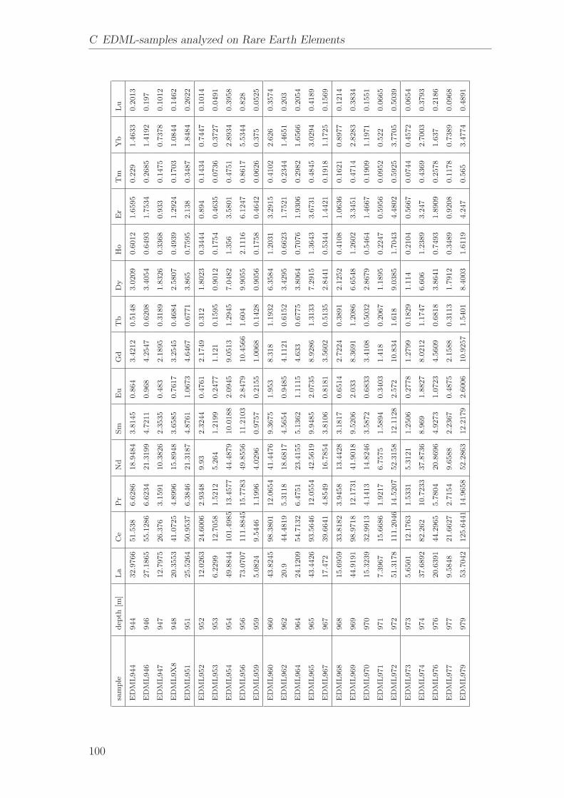
C EDML-samples analyzed on Rare Earth Elements
sam
ple
dep
th[m
]La
Ce
Pr
Nd
Sm
Eu
Gd
Tb
Dy
Ho
Er
Tm
Yb
Lu
ED
ML944
944
32.9
766
51.5
38
6.6
286
18.9
484
3.8
145
0.8
64
3.4
212
0.5
148
3.0
209
0.6
012
1.6
595
0.2
29
1.4
633
0.2
013
ED
ML946
946
27.1
865
55.1
286
6.6
234
21.3
199
4.7
211
0.9
68
4.2
547
0.6
208
3.4
054
0.6
493
1.7
534
0.2
685
1.4
192
0.1
97
ED
ML947
947
12.7
975
26.3
76
3.1
591
10.3
826
2.3
535
0.4
83
2.1
895
0.3
189
1.8
326
0.3
368
0.9
33
0.1
475
0.7
378
0.1
012
ED
ML9X
8948
20.3
553
41.0
725
4.8
996
15.8
948
3.6
585
0.7
617
3.2
545
0.4
684
2.5
807
0.4
939
1.2
924
0.1
703
1.0
844
0.1
462
ED
ML951
951
25.5
264
50.9
537
6.3
846
21.3
187
4.8
761
1.0
673
4.6
467
0.6
771
3.8
65
0.7
595
2.1
38
0.3
487
1.8
484
0.2
622
ED
ML952
952
12.0
263
24.6
006
2.9
348
9.9
32.3
244
0.4
761
2.1
749
0.3
12
1.8
023
0.3
444
0.8
94
0.1
434
0.7
447
0.1
014
ED
ML953
953
6.2
299
12.7
058
1.5
212
5.2
64
1.2
199
0.2
477
1.1
21
0.1
595
0.9
012
0.1
754
0.4
635
0.0
736
0.3
727
0.0
491
ED
ML954
954
49.8
844
101.4
985
13.4
577
44.4
879
10.0
188
2.0
945
9.0
513
1.2
945
7.0
482
1.3
56
3.5
801
0.4
751
2.8
934
0.3
958
ED
ML956
956
73.0
707
111.8
845
15.7
783
49.8
556
11.2
103
2.8
479
10.4
566
1.6
04
9.9
055
2.1
116
6.1
247
0.8
617
5.5
344
0.8
28
ED
ML959
959
5.0
824
9.5
446
1.1
996
4.0
296
0.9
757
0.2
155
1.0
068
0.1
428
0.9
056
0.1
758
0.4
642
0.0
626
0.3
75
0.0
525
ED
ML960
960
43.8
245
98.3
801
12.0
654
41.4
476
9.3
675
1.9
53
8.3
18
1.1
932
6.3
584
1.2
031
3.2
915
0.4
102
2.6
26
0.3
574
ED
ML962
962
20.9
44.4
819
5.3
118
18.6
817
4.5
654
0.9
485
4.1
121
0.6
152
3.4
295
0.6
623
1.7
521
0.2
344
1.4
651
0.2
03
ED
ML964
964
24.1
209
54.7
132
6.4
751
23.4
155
5.1
362
1.1
115
4.6
33
0.6
775
3.8
064
0.7
076
1.9
306
0.2
982
1.6
566
0.2
054
ED
ML965
965
43.4
426
93.5
646
12.0
554
42.5
619
9.9
485
2.0
735
8.9
286
1.3
133
7.2
915
1.3
643
3.6
731
0.4
845
3.0
294
0.4
189
ED
ML967
967
17.4
72
39.6
641
4.8
549
16.7
854
3.8
106
0.8
181
3.5
602
0.5
135
2.8
441
0.5
344
1.4
421
0.1
918
1.1
725
0.1
569
ED
ML968
968
15.6
959
33.8
182
3.9
458
13.4
428
3.1
817
0.6
514
2.7
224
0.3
891
2.1
252
0.4
108
1.0
636
0.1
621
0.8
977
0.1
214
ED
ML969
969
44.9
191
98.9
718
12.1
731
41.9
018
9.5
206
2.0
33
8.3
691
1.2
086
6.6
548
1.2
602
3.3
451
0.4
714
2.8
283
0.3
834
ED
ML970
970
15.3
239
32.9
913
4.1
413
14.8
246
3.5
872
0.6
833
3.4
108
0.5
032
2.8
679
0.5
464
1.4
667
0.1
909
1.1
971
0.1
551
ED
ML971
971
7.3
967
15.6
686
1.9
217
6.7
575
1.5
894
0.3
403
1.4
18
0.2
067
1.1
895
0.2
247
0.5
956
0.0
952
0.5
22
0.0
665
ED
ML972
972
51.3
178
111.2
046
14.5
207
52.3
158
12.1
128
2.5
72
10.8
34
1.6
18
9.0
385
1.7
043
4.4
802
0.5
925
3.7
705
0.5
039
ED
ML973
973
5.6
501
12.1
763
1.5
331
5.3
121
1.2
506
0.2
778
1.2
799
0.1
829
1.1
14
0.2
104
0.5
667
0.0
744
0.4
572
0.0
654
ED
ML974
974
37.6
892
82.2
62
10.7
233
37.8
736
8.9
69
1.8
827
8.0
212
1.1
747
6.6
06
1.2
389
3.2
47
0.4
369
2.7
003
0.3
793
ED
ML976
976
20.6
391
44.2
965
5.7
804
20.8
696
4.9
273
1.0
723
4.5
609
0.6
818
3.8
641
0.7
493
1.8
909
0.2
578
1.6
37
0.2
186
ED
ML977
977
9.5
848
21.6
627
2.7
154
9.6
588
2.2
367
0.4
875
2.1
588
0.3
113
1.7
912
0.3
489
0.9
208
0.1
178
0.7
389
0.0
968
ED
ML979
979
53.7
042
125.6
441
14.9
658
52.2
863
12.2
179
2.6
006
10.9
257
1.5
401
8.4
003
1.6
119
4.2
47
0.5
65
3.4
774
0.4
891
100

sam
ple
dep
th[m
]La
Ce
Pr
Nd
Sm
Eu
Gd
Tb
Dy
Ho
Er
Tm
Yb
Lu
ED
ML980
980
51.9
878
114.4
234
15.7
562
54.2
515
12.8
007
2.6
284
11.4
95
1.6
904
9.2
884
1.7
854
4.6
711
0.6
223
3.8
381
0.5
234
ED
ML983
983
18.7
013
39.8
668
4.8
557
17.6
538
4.4
368
0.8
753
4.1
742
0.6
106
3.5
06
0.6
763
1.8
032
0.2
395
1.4
947
0.2
052
ED
ML984
984
17.7
05
38.8
549
4.7
592
17.2
832
3.9
923
0.8
176
3.6
551
0.5
206
2.9
396
0.5
526
1.4
525
0.2
277
1.2
34
0.1
669
ED
ML986
986
41.6
407
93.4
313
11.4
071
41.0
725
9.6
866
2.0
092
8.7
83
1.2
783
7.0
805
1.3
388
3.5
387
0.5
534
2.9
44
0.4
066
ED
ML987
987
20.0
285
43.0
076
5.3
254
19.0
99
4.5
418
0.9
261
4.0
53
0.5
947
3.3
524
0.6
266
1.6
677
0.2
239
1.4
032
0.1
866
ED
ML989
989
43.6
645
98.3
69
12.4
724
44.6
784
10.5
893
2.2
303
9.3
813
1.3
473
7.4
27
1.4
217
3.6
857
0.4
891
3.1
011
0.4
276
ED
ML991
991
7.1
01
16.7
634
2.0
626
7.5
356
1.7
041
0.3
631
1.7
013
0.2
449
1.4
358
0.2
765
0.7
354
0.0
965
0.5
95
0.0
803
ED
ML992
992
2.5
635
6.1
693
0.6
696
2.4
885
0.5
89
0.1
17
0.5
018
0.0
646
0.4
161
0.0
746
0.2
071
0.0
315
0.1
711
0.0
178
ED
ML993
993
7.5
121
17.0
122
2.1
447
7.7
502
1.9
061
0.4
053
1.7
556
0.2
51.4
624
0.2
808
0.7
546
0.1
008
0.6
201
0.0
846
ED
ML994
994
4.8
641
10.6
731
1.3
217
4.7
712
1.1
178
0.2
567
1.1
919
0.1
735
1.0
375
0.1
993
0.5
417
0.0
707
0.4
555
0.0
574
ED
ML997
997
14.7
618
34.1
141
4.3
515.5
618
3.7
434
0.7
18
3.6
497
0.5
164
2.9
089
0.5
505
1.4
857
0.1
956
1.2
259
0.1
581
ED
ML1004
1004
37.4
833
83.0
839
9.8
081
34.8
171
8.1
088
1.6
68
7.1
676
1.0
401
5.6
015
1.0
541
2.7
695
0.4
366
2.3
171
0.3
433
ED
ML1007
1007
11.1
303
25.3
737
3.1
55
10.9
371
2.5
087
0.5
103
2.3
55
0.3
299
1.8
871
0.3
585
0.9
675
0.1
312
0.7
95
0.1
066
ED
ML1009
1009
5.2
197
11.8
459
1.4
472
5.1
127
1.1
649
0.2
519
1.1
765
0.1
667
0.9
586
0.1
857
0.5
008
0.0
662
0.4
058
0.0
507
ED
ML1012
1012
2.5
191
5.6
562
0.6
95
2.4
243
0.5
542
0.1
17
0.5
744
0.0
792
0.4
942
0.0
972
0.2
662
0.0
346
0.2
144
0.0
261
ED
ML1013
1013
58.4
368
137.0
46
16.3
64
57.4
968
13.0
531
2.6
577
11.4
556
1.6
233
8.8
94
1.6
73
4.4
354
0.6
3.7
25
0.5
071
ED
ML1014
1014
8.1
689
18.3
905
2.1
693
7.8
054
1.9
049
0.3
996
1.6
167
0.2
413
1.2
865
0.2
456
0.6
38
0.1
03
0.5
246
0.0
736
ED
ML1016
1016
10.3
527
22.6
917
2.8
89
10.9
673
2.3
63
0.5
064
2.2
30.3
183
1.8
464
0.3
458
0.9
341
0.1
206
0.7
497
0.1
004
ED
ML1019
1019
2.6
349
5.7
942
0.6
778
2.4
616
0.6
755
0.1
513
0.5
549
0.0
758
0.4
559
0.0
897
0.2
394
0.0
376
0.1
90.0
234
ED
ML1020
1020
3.3
63
7.5
03
0.9
406
3.3
391
0.7
69
0.1
696
0.8
066
0.1
102
0.6
757
0.1
315
0.3
637
0.0
452
0.2
899
0.0
334
ED
ML1021
1021
15.8
238
35.2
582
4.2
699
15.5
823
3.7
205
0.7
417
3.2
405
0.4
752
2.7
181
0.4
888
1.3
496
0.1
791
1.1
238
0.1
537
ED
ML1022
1022
5.7
745
13.1
033
1.5
866
5.7
507
1.3
167
0.2
789
1.3
053
0.1
839
1.0
383
0.1
988
0.5
374
0.0
704
0.4
464
0.0
549
ED
ML1024
1024
27.4
021
58.5
423
7.6
847
27.6
129
6.4
206
1.3
421
5.8
063
0.8
383
4.7
273
0.8
726
2.3
391
0.3
034
1.9
274
0.2
614
ED
ML1027
1027
5.2
965
9.8
97
1.2
189
4.0
904
0.9
908
0.2
28
0.9
335
0.1
321
0.8
142
0.1
623
0.4
232
0.0
684
0.3
506
0.0
517
ED
ML1030
1030
10.7
743
23.3
873
2.9
75
10.9
123
2.5
93
0.5
35
2.3
754
0.3
41
2.0
168
0.3
704
1.0
24
0.1
38
0.8
427
0.1
13
101

C EDML-samples analyzed on Rare Earth Elements
sam
ple
dep
th[m
]La
Ce
Pr
Nd
Sm
Eu
Gd
Tb
Dy
Ho
Er
Tm
Yb
Lu
ED
ML1031
1031
6.4
423
13.6
304
1.7
293
6.3
018
1.5
004
0.3
139
1.4
134
0.1
986
1.1
791
0.2
302
0.6
173
0.0
784
0.5
156
0.0
668
ED
ML1033
1033
1.3
798
3.1
582
0.3
715
1.3
925
0.3
22
0.0
663
0.3
353
0.0
416
0.2
968
0.0
568
0.1
527
0.0
205
0.1
268
0.0
138
ED
ML1036
1036
33.3
907
74.1
202
9.4
708
33.9
027
8.0
456
1.6
625
7.2
607
1.0
62
5.8
254
1.1
216
3.0
382
0.3
871
2.4
645
0.3
451
ED
ML1038
1038
3.4
886
7.2
976
0.9
138
3.2
634
0.7
159
0.1
572
0.7
442
0.1
003
0.6
493
0.1
341
0.3
599
0.0
486
0.3
082
0.0
385
ED
ML1039
1039
34.1
156
73.7
848
9.6
768
34.1
607
8.1
528
1.6
947
7.2
222
1.0
371
5.9
045
1.0
962
2.8
808
0.3
865
2.4
775
0.3
328
ED
ML1040
1040
5.4
64
12.7
078
1.5
499
5.6
699
1.3
087
0.2
706
1.2
383
0.1
806
1.0
336
0.1
961
0.5
206
0.0
687
0.4
19
0.0
547
ED
ML1041
1041
14.6
432
30.4
588
3.7
012
12.8
63.0
09
0.6
506
2.7
341
0.4
002
2.3
021
0.4
472
1.2
435
0.1
632
0.9
911
0.1
397
ED
ML1042
1042
8.1
545
17.0
242
2.1
187
7.7
329
1.7
376
0.3
677
1.6
547
0.2
337
1.3
163
0.2
524
0.6
834
0.0
916
0.5
594
0.0
684
ED
ML1043
1043
32.3
07
36.4
972
0.7
138
1.8
109
0.3
087
0.0
712
0.2
775
0.0
372
0.2
601
0.0
551
0.1
555
0.0
254
0.1
388
0.0
17
ED
ML1044
1044
7.0
183
15.6
408
1.8
452
6.6
197
1.6
113
0.3
492
1.4
953
0.2
093
1.2
311
0.2
316
0.6
176
0.0
891
0.4
968
0.0
681
ED
ML1046
1046
18.4
924
42.2
542
5.1
121
18.1
989
4.2
584
0.9
07
3.8
933
0.5
628
3.0
694
0.5
938
1.5
835
0.2
121
1.3
169
0.1
849
ED
ML1047
1047
12.8
661
25.4
361
3.2
356
11.6
389
2.5
999
0.6
038
2.4
656
0.3
533
2.1
412
0.4
31.1
531
0.1
642
1.0
319
0.1
381
ED
ML1048
1048
20.7
535
47.6
563
5.7
76
20.9
434
4.8
543
1.0
204
4.3
792
0.6
23
3.4
375
0.6
601
1.7
35
0.2
318
1.3
894
0.1
943
ED
ML1049
1049
23.3
529
53.1
146
6.6
625
23.5
488
5.5
809
1.1
914
5.1
536
0.7
27
4.0
171
0.7
379
2.0
028
0.2
705
1.7
096
0.2
198
ED
ML1050
1050
12.7
328
27.1
124
3.4
031
12.1
95
2.8
871
0.6
108
2.7
251
0.3
943
2.2
461
0.4
321
1.1
246
0.1
523
0.9
288
0.1
305
ED
ML1051
1051
15.6
058
35.0
447
4.2
844
15.3
325
3.5
74
0.7
931
3.2
205
0.4
598
2.5
208
0.4
81
1.2
654
0.1
721
1.0
543
0.1
423
ED
ML1052
1052
37.5
401
82.1
608
10.8
189
39.0
419
9.1
285
1.8
937
8.4
271
1.2
333
6.7
255
1.2
722
3.3
156
0.4
45
2.7
675
0.3
867
ED
ML1053
1053
7.4
352
15.8
916
1.9
479
7.1
671
1.6
764
0.3
577
1.5
993
0.2
35
1.3
655
0.2
596
0.7
016
0.0
912
0.6
011
0.0
777
ED
ML1054
1054
26.1
715
60.8
603
7.2
878
26.3
065
6.0
538
1.3
02
5.4
904
0.7
857
4.2
286
0.8
084
2.1
726
0.2
939
1.8
279
0.2
503
ED
ML1056
1056
11.8
315
25.8
319
3.2
499
12.0
122
2.8
673
0.6
046
2.6
647
0.3
742
2.2
106
0.4
043
1.0
89
0.1
474
0.8
968
0.1
167
ED
ML1057
1057
6.3
74
14.8
139
1.8
172
6.5
906
1.5
457
0.3
28
1.4
881
0.2
098
1.2
111
0.2
312
0.6
147
0.0
823
0.5
134
0.0
648
ED
ML1059
1059
9.5
978
23.1
496
2.7
22
9.8
239
2.2
911
0.4
639
2.1
515
0.2
984
1.6
824
0.3
173
0.8
533
0.1
129
0.7
134
0.0
924
ED
ML1061
1061
40.3
454
98.7
149
11.0
717
38.1
604
9.4
653
1.9
292
7.8
908
1.1
18
5.9
534
1.1
092
2.7
907
0.4
566
2.4
803
0.3
576
ED
ML1062
1062
11.8
205
25.1
22
3.0
134
10.3
992
2.3
34
0.5
02
2.0
082
0.2
94
1.6
183
0.3
207
0.8
49
0.1
162
0.7
091
0.0
933
ED
ML1063
1063
35.7
217
85.6
836
9.8
074
34.5
036
8.1
267
1.6
792
6.8
549
0.9
945
5.2
678
0.9
84
2.5
899
0.4
113
2.2
496
0.3
208
102

sam
ple
dep
th[m
]La
Ce
Pr
Nd
Sm
Eu
Gd
Tb
Dy
Ho
Er
Tm
Yb
Lu
ED
ML1064
1064
45.3
679
115.2
298
12.8
403
44.2
453
10.4
659
2.2
637
8.8
147
1.2
789
6.7
795
1.3
054
3.2
387
0.5
045
2.7
451
0.3
995
ED
ML1066
1066
58.2
139
132.4
508
16.0
95
58.6
075
13.5
044
2.7
648
11.5
389
1.6
902
9.2
935
1.7
151
4.6
043
0.6
282
3.9
687
0.5
345
ED
ML1067
1067
25.8
234
57.4
226
7.2
245
25.6
712
6.0
939
1.2
607
5.3
817
0.7
829
4.3
703
0.8
05
2.1
775
0.2
903
1.8
511
0.2
51
ED
ML1068
1068
42.2
729
98.1
043
11.2
538
40.8
544
9.8
31.9
292
8.2
55
1.1
868
6.4
746
1.2
13
3.2
252
0.4
281
2.7
463
0.3
722
ED
ML1069
1069
38.2
718
87.5
227
10.6
168
38.2
367
8.9
405
1.8
308
7.9
004
1.1
456
6.3
11
1.1
993
3.1
714
0.4
308
2.6
628
0.3
571
ED
ML1070
1070
20.8
416
44.0
55.6
657
20.4
734
4.7
922
0.9
873
4.3
284
0.6
318
3.5
621
0.6
779
1.7
637
0.2
369
1.4
525
0.1
987
ED
ML1073
1073
9.1
388
21.6
79
2.6
311
9.4
921
2.1
725
0.4
273
1.9
801
0.2
759
1.5
893
0.3
034
0.8
056
0.1
07
0.6
618
0.0
856
ED
ML1076
1076
87.0
511
208.8
407
23.4
295
83.1
602
19.6
935
4.2
82
16.0
615
2.3
749
13.1
535
2.2
96.3
89
0.9
638
5.2
625
0.7
849
ED
ML1078
1078
12.3
184
21.6
476
2.8
049
9.3
683
2.1
519
0.4
602
1.9
677
0.2
843
1.5
992
0.3
221
0.8
645
0.1
192
0.7
118
0.1
013
ED
ML1080
1080
68.5
74
153.3
802
20.5
33
72.4
26
16.8
192
3.4
709
15.1
851
2.2
298
11.8
384
2.2
968
5.9
802
0.7
964
4.8
934
0.7
017
ED
ML1082
1082
37.6
605
86.5
088
10.7
372
39.0
001
8.9
529
1.8
796
8.1
626
1.1
634
6.4
172
1.2
168
3.1
963
0.4
276
2.6
68
0.3
674
ED
ML1084
1084
101.4
322
237.0
254
28.3
482
100.5
44
23.0
715
4.8
969
20.2
896
2.9
863
16.1
372
2.9
847
8.0
123
1.2
459
6.5
672
0.9
576
ED
ML1086
1086
27.7
224
64.4
931
7.1
298
25.6
431
5.9
892
1.2
88
5.1
851
0.7
259
3.9
44
0.7
472
1.9
388
0.3
009
1.6
043
0.2
333
ED
ML1088
1088
88.1
203
204.5
831
23.3
006
83.4
666
19.7
089
4.1
279
17.2
204
2.5
109
13.4
098
2.5
965
6.7
049
1.0
408
5.6
77
0.8
094
ED
ML1090
1090
13.3
692
30.7
903
3.5
09
12.8
756
3.0
193
0.6
096
2.6
104
0.3
627
2.0
221
0.3
727
1.0
104
0.1
376
0.8
272
0.1
164
ED
ML1093
1093
17.3
31
38.6
909
4.7
668
17.1
57
4.0
108
0.8
238
3.4
923
0.4
903
2.7
821
0.5
322
1.3
924
0.1
92
1.2
039
0.1
604
ED
ML1096
1096
39.9
619
92.1
794
11.9
369
43.0
608
9.9
18
2.0
924
9.3
237
1.3
219
7.3
17
1.3
781
3.6
938
0.4
958
3.1
364
0.4
164
ED
ML1097
1097
34.1
287
79.8
02
9.5
584
34.7
638
7.8
639
1.6
583
7.1
188
1.0
236
5.6
421
1.0
838
2.8
658
0.3
606
2.4
037
0.3
353
ED
ML1099
1099
32.8
417
72.2
811
9.4
331
33.7
185
7.9
102
1.6
878
7.2
696
1.0
434
5.6
792
1.0
858
2.9
359
0.3
85
2.4
142
0.3
463
ED
ML1100
1100
42.1
562
100.2
088
11.2
904
41.9
976
9.8
704
2.1
524
8.5
344
1.2
14
6.5
164
1.2
349
3.2
664
0.5
282
2.6
537
0.4
206
ED
ML1101
1101
9.8
256
21.9
729
2.6
237
9.5
507
2.3
591
0.5
103
2.1
239
0.3
01
1.6
675
0.3
281
0.8
535
0.1
301
0.6
84
0.0
969
ED
ML1104
1104
37.6
263
85.4
863
10.3
837
38.3
066
8.7
753
1.7
977
7.5
617
1.0
926
6.1
296
1.1
607
3.0
151
0.4
135
2.6
155
0.3
502
ED
ML1105
1105
49.1
481
120.1
977
13.6
118
50.5
654
11.7
038
2.4
72
10.0
186
1.4
967
7.9
94
1.5
16
3.9
484
0.6
445
3.3
506
0.4
795
Tab
leC
.1:
Nam
es,de
pths
and
RE
Eco
ncen
trat
ion
[ng·L
−1]of
the
ice
core
sam
ples
anal
yzed
inth
isst
udy.
bdl:
conc
entr
atio
nw
asbe
low
dete
ctio
nlim
it.
103

D Samples from the Potential Source Areas
sample name continent geographical coordinates remarksA1 Antarctica 77◦43’ S, 161◦23’ E -A2 Antarctica 77◦31’ S, 169◦24’ E -A3 Antarctica 77◦17’ S, 193◦15’ E -A4 Antarctica 77◦17’ S, 163◦15’ E -A5 Antarctica 77◦30’ S, 165◦0’ E -A6 Antarctica 77◦30’ S, 165◦0’ E -A7 Antarctica 77◦37’ S, 163◦11’ E -A8 Antarctica 77◦38’ S, 162◦51’ E -A9 Antarctica 77◦28’ S, 161◦42’ E -A10 Antarctica 77◦50’ S, 164◦30’ E -NZ22 New Zealand 44◦38’ S, 168◦59’ E -NZ12 New Zealand 45◦24’ S, 167◦42’ E -NZ31 New Zealand - -NZ32 New Zealand - -NZ143 New Zealand 43◦28’ S, 172◦31’ E -Na1 Southern Africa 24◦29’ S, 15◦48’ E -Na2 Southern Africa 24◦42’ S, 15◦17’ E -Na3 Southern Africa 23◦7’ S, 14◦30’ E -Na4 Southern Africa 24◦42’ S, 15◦17’ E -SouthafricanAerosol
southern Africa 33.5◦’ S, 22◦0’ W -
Table D.1: Samples from the PSA of Antarctic ice core dust analyzed in this study. Continued onnext page.
104

sam
ple
nam
eco
ntin
ent
geog
raph
ical
coor
dina
tes
rem
arks
Aus
Aus
tral
ia25
◦ 20’
S,13
1◦2’
EA
yers
Roc
k,N
orth
ern
Ter
rito
ryA
RLO
Z5
Sout
hA
mer
ica
31◦ 3
9’S,
64◦ 8
’W
Cor
doba
area
,10
-20
kaB
.PA
RB
AR
4So
uth
Am
eric
a33
◦ 49’
S,59
◦ 31’
WPam
pas,
ca.
20ka
B.P
AR
HU
D3
Sout
hA
mer
ica
25km
NW
from
AR
GO
R2
Pam
pas,
¡23
kaB
.PA
RG
OR
2So
uth
Am
eric
a34
◦ 54’
S,58
◦ 1’W
Pam
pas,
20-
25ka
B.P
AR
MD
P1
Sout
hA
mer
ica
37◦ 5
7’S,
57◦ 3
8’W
Pam
pas,
20-
25ka
B.P
CH
1So
uth
Am
eric
a41
◦ 9’S,
71◦ 1
8’W
San
Car
los
deB
arilo
che,
Arg
enti
naye
llow
silt
,lo
ess-
like
CH
5So
uth
Am
eric
a48
◦ 38’
S,74
◦ 6’W
wes
tern
coas
tof
Isla
Gra
nde
deC
hilo
eda
rkgr
eysa
nd,m
oder
nae
olia
nde
posi
tC
H6
Sout
hA
mer
ica
51◦ 4
’S,
73◦ 9
’W
fron
talm
orai
ne,50
-60
mab
ove
the
leve
lof
Lak
eG
rey,
torr
ede
lPai
neN
atio
nalPar
k,gr
eysa
ndC
H8
Sout
hA
mer
ica
-C
H9
Sout
hA
mer
ica
53◦ 9
’S,
70◦ 5
5’W
prob
able
abo
ttom
mor
aine
buri
edun
der
a30
-40
cmso
illig
htol
ive
brow
nsi
ltw
ith
brow
nish
patc
hes
CH
10So
uth
Am
eric
a53
◦ 18’
S,70
◦ 22’
Wbo
ttom
mor
aine
,T
ierr
ade
lFu
ego,
light
brow
nish
gray
silt
wit
hsa
lty
encr
usta
tion
sfr
omm
arin
eae
roso
lC
H11
Sout
hA
mer
ica
53◦ 9
’S,
70◦ 5
5’W
4.5
kmw
est
ofP
unta
Are
nas
yello
wis
h-br
own
sand
ysi
lt(l
oess
-lik
e)B
ahia
Bla
nca
Sout
hA
mer
ica
28◦ 4
4’S,
62◦ 1
6’W
-Pat
agon
iaSo
uth
Am
eric
a-
-
Tab
leD
.2:
Sam
ples
from
the
PSA
ofA
ntar
ctic
ice
core
dust
anal
yzed
inth
isst
udy.
Con
tinu
edfr
omla
stpa
ge.
105

E Mathematics of the PCA
The PCA is performed on the REE without the element Pm, since Pm does nothave any stable isotope and could therefore not be measured.
1. Center the matrix used for the PCA X → Xmean = X − mean(X)
2. Compute the covariance matrix S → S = X ′mean · Xmean
3. Compute eigenvector matrix F and eigenvalues L of S.
4. Sort eigenvectors and eigenvalues in decreasing order of eigenvalues.
5. Calculate principal components B → B = X · F . B gives the coordinates inthe new coordinate system CSPC .
6. Transform the other samples, that were not used for the initial PCA Xall, inthe new coordinate system CSPC
• Center the data Xall → Xallcenter = Xall − mean(X)
• Transform the samples into CSPC → Ball = Xallcenter · F
106

F Derivation of Dust Size Distribution ChangesDuring Transport
Change of the concentration within one size interval.Assumptions:
• no interaction between individual size classes
• deposition is caused by wet and dry deposition and proportional to the particleconcentration
Hdcair(d, t)
dt= −cair[vdry + vwet] (F.1)
vdry = kd2 (F.2)
vwet = εA(t) (F.3)
with Equation F.1, Equation F.2 and Equation F.3
Hdcair(d, t)
dt= −cair[kd2 + εA(t)] | : H| · dt| : cair (F.4)
dcair(d, t)
cair
= −kd2 + εA(t)
Hdt |
∫(F.5)
ln(cair(d,t)) = −kd2t + ε∫
A(t)dt
H|exp (F.6)
cair(d,t) = cair,0 · e−kd2t+ε
RA(t)dt
H (F.7)
Assuming A(t) constant during en route simplifies∫
A(t)dt to εAt, leading to
cair(d,t) = cair,0 · e− kd2t+εAtH (F.8)
Change of concentration in a log-normal size distribution with independentparticle channels.
107

F Derivation of Dust Size Distribution Changes During Transport
V (t, logd) =a0√
2πlogσ0
e− 1
2(logd−logμ0)2
log2σ0 (F.9)
Change of the concentration during the transport according to Equation F.7
V (t, logd) = V (t = 0, logd)e−kd2
Ht− ε
HAt (F.10)
With Equation F.9 and Equation F.10
V (t, logd) =a0√
2πlogσ0
e− 1
2(logd−logμ0)2
log2σ0− kd2
Ht− ε
HAt
(F.11)
The maximum of this equation (d = μair) is deduced by setting the first derivativewith respect to logd to zero.
dV (t, log(d = μair))
dlogd= 0 (F.12)
dV (t, log(d = μair))
dlogd=
P0√2πlogσ0
· e− 12(
logμair−logμ0logσ0
)2− tH
(kd2+εA)· (F.13)
[ logd−logμ0
log2σ0− (2 t
Hkd2ln10)] = 0
While generating the derivative of d with respect to logd the relationd = 10logd = elogd·ln10
was used.
In Equation F.13 e− 1
2(
logd−logμ0logσ0
)2− tH
(kd2+εA)is always �= 0. This means for fulfilling
dV (t,logd)dlogd
= 0 is obtained with
logd − logμ0
log2σ0
− (2t
Hkd2ln10) = 0. (F.14)
logd − logμ0
log2σ0
= −2ln10kd2 t
H| · log2σ0 (F.15)
with d = μair
logμair − logμ0 = logμair
μ0
= −2ln10kμ2air
t
H· log2σ0 (F.16)
Taking 2 different stages I and II and subtracting Equation F.16 for stage II fromEquation F.16 for stage I
108

logμI
air
μ0
− μIIair
μ0
= −2ln10kμIair
2 tI
H· log2σ0 + 2ln10kμII
air
2 tII
H· log2σ0 (F.17)
Assuming H, μ0, σ0 and k to be constant from stage I and II
logμI
air
μIIair
= −2ln10klog2σ0
H(μI
air
2tI − μII
air
2tII) (F.18)
Using Equation F.16
logμI
air
μIIair
= logμI
air
μ0
(1 − μIIair
2
μIair
2
tII
tI) (F.19)
109

G Dust Concentration Blank Levels
Blank levels during the measurements with the Coulter Counter
sample EDML1083 EDML746Particle Diameter mean stddev mean stddev
[μm] [part/ml] [part/ml] [part/ml] [part/ml]< 1 354.1 249.6 52.2 48.51 - 2 316.0 224.3 58.4 53.52 - 3 40.3 34.8 9.2 13.43 - 4 9.6 12.1 1.6 4.84 - 5 3.3 8.1 1.1 3.75 - 6 0.8 2.6 0.4 1.96 - 7 0.4 1.9 0.4 1.97 - 8 0.0 0.0 0.2 1.38 - 9 0.3 1.9 0.0 0.09 - 10 0.3 1.9 0.1 0.410 - 11 0.0 0.0 0.1 1.011 - 18 0.0 0.0 0.4 1.9
number of blanks 41 55
Table G.1: Blank levels of the Coulter Counter measurements

Bibliography
[Adam and Green, 1993] Adam, J. and Green, T. H. (1993). The effect of pres-sure and temperature on the partitioning of Ti, Sr and REE between amphibole,clinopyroxene and basaltic melts. Chemical Geology, 117:219–233.
[Albarede, 2003] Albarede, F. (2003). Geochemistry: An Introduction. CambridgeUniversity Press, Cambridge.
[Alfaro and Gomes, 2001] Alfaro, C. A. and Gomes, L. (2001). Modeling mineralaerosol production by wind erosion: Emission intensities and aerosol size distri-butions in source areas. Journal of Geophysical Research, 106:18075–18084.
[Arimoto, 2001] Arimoto, R. (2001). Eolian dust and climate: relationships tosources, tropospheric chemistry, transport and deposition. Earth-Science Reviews,54:29–42.
[Basile et al., 1997] Basile, I., Grousset, F., Revel, M., Petit, J. R., Biskaye, P. E.,and Barkov, N. I. (1997). Patagonian origin of glacial dust deposited in EastAntarctica (Vostok and Dome C) during glacial stages 2, 4 and 6. Earth andPlanetary Science Letters, 146:573 – 589.
[Beer et al., 1988] Beer, J., Siegenthaler, U., Bonani, G., Finkel, R. C., Oeschger,H., Suter, M., and Wolfli, W. (1988). Information on past solar activity andgeomagnetism from 10Be in the Camp Century ice core. Nature, 331:675–679.
[Beer et al., 2006] Beer, J., Vonmoos, M., and Muscheler, R. (2006). Solar variabil-ity over the past several millennia. Space Science Reviews, 125:67–79.
[Biscaye et al., 1997] Biscaye, P. E., Grousset, F. E., Revel, M., Van der Gaast, S.,Zielinski, G. A., Vaars, A., and Kukla, G. (1997). Asian provenance of glacialdust (stage 2) in the Greenland Ice Sheet Project 2 ice core, Summit, Greenland.Journal of Geophysical Research, 102:26765–26781.
[Blunier et al., 1998] Blunier, T., Chappellaz, J., Schwander, J., Dallenbach, A.,Stauffer, B., Stocker, T. F., Raynaud, D., Jouzel, J., Clausen, H. B., Hammer,C. U., and Johnsen, S. J. (1998). Asynchrony of Antarctic and Greenland climatechange during the last glacial period. Nature, 394:739–743.
[Buseck and Veblen, 1978] Buseck, P. R. and Veblen, D. R. (1978). Trace ele-ments, crystal defects and high resolution electron microscopy. Geochimica etCosmochimica Acta, 42(6):669–678.
[Claquin et al., 1999] Claquin, T., Schulz, M., and Balkanski, Y. J. (1999). Modelingthe mineralogy of atmospheric dust sources. Journal of Geophysical Research,104:22243–22256.
111

Bibliography
[Coulter, 1959] Coulter, W. (1959). Fluid metering apparatus. US. Patent No.2869078.
[de Angelis et al., 1984] de Angelis, M., Legrand, M., Petit, J. R., Barkov, N. I.,Korotkevitch, Y. S., and Kotlyalov (1984). Soluble and Isoluble Impurities Alongthe 950 m Deep Vostok Ice Core (Antarctica) - Climatic Implications. Journal ofAtmospheric Chemistry, 1:215–239.
[Delmonte, 2003] Delmonte, B. (2003). Quaternary variations and origin of con-tinental dust in east Antarctica. PhD thesis, Universita degli Studi di Milano-Bicocca.
[Delmonte et al., 2002a] Delmonte, B., Basile-Doelsch, I., Michard, A., Petit, J. R.,Maggi, V., Gemmiti, B., and Revel-Rolland, M. (2002a). Sr-Nd signature of po-tential source areas for dust in East Antarctica: Preliminary results. Geochimicaet Cosmochimica Acta, 66(15A):A175–A175.
[Delmonte et al., 2004a] Delmonte, B., Basile-Doelsch, I., Petit, J. R., Maggi, V.,Revel-Rolland, M., Michard, A., Jagoutz, E., and Grousset, F. (2004a). Com-paring the Epica and Vostok dust records during the last 220,000 years: strati-graphical correlation and provenance in glacial periods. Earth-Science Reviews,66(1-2):63–87.
[Delmonte et al., 2004b] Delmonte, B., Petit, J. R., Andersen, K. K., Basile-Doelseh, I., Maggi, V., and Lipenkov, V. Y. (2004b). Dust size evidence foropposite regional atmospheric circulation changes over east Antarctica during thelast climatic transition. Climate Dynamics, 23(3-4):427–438.
[Delmonte et al., 2005] Delmonte, B., Petit, J. R., Krinner, G., Maggi, V., Jouzel,J., and Udisti, R. (2005). Ice core evidence for secular variability and 200-yeardipolar oscillations in atmospheric circulation over East Antarctica during theHolocene. Climate Dynamics, 24(6):641–654.
[Delmonte et al., 2002b] Delmonte, B., Petit, J. R., and Maggi, V. (2002b). Glacialto Holocene implications of the new 27000-year dust record from the EPICA DomeC (East Antarctica) ice core. Climate Dynamics, 18(8):647–660.
[Dentener et al., 1996] Dentener, F. J., R., C. G., Zhang, Y., Lelieveld, J., andCrutzen, P. J. (1996). Role of mineral aerosol as a reactive surface in the globaltroposphere. Journal of Geophysical Research, 101:22869–22890.
[Duce, 1995] Duce, R. A. (1995). Aerosol forcing of Climate, chapter Sources, Dis-tributions, and Fluxes of Mineral Aerosol anf Their relationship to Climate, pages43–72. Report of Dahlem Workshop.
[EPICA Community Members, 2004] EPICA Community Members (2004). Eightglacial cycles from an Antarctic ice core. Nature, 429(6992):623–628.
[EPICA Community Members, 2006] EPICA Community Members (2006). One-to-one coupling of glacial climate variability in Greenland and Antarctica. Nature,444(7116):195–198.
112

Bibliography
[Feichter, 2003] Feichter, J. (2003). Aerosole und das Klimasystem. Physik in un-serer Zeit, 34:72–79.
[Fischer et al., 2007a] Fischer, H., Fundel, F., Ruth, U., Twarloh, B., Wegner, A.,Udisti, R., Becagli, S., Castellano, E., Morganti, A., Severi, M., Wolff, E., Littot,G., Rothlisberger, R., Mulvaney, R., Hutterli, M. A., Kaufmann, P., Federer, U.,Lambert, F., Bigler, M., Hansson, M., Jonsell, U., de Angelis, M., Boutron, C.,Siggaard-Andersen, M. L., Steffensen, J. P., Barbante, C., Gaspari, V., Gabrielli,P., and Wagenbach, D. (2007a). Reconstruction of millenial changes in the dustemission, transport and regional sea ice coverage using the deep EPICA ice coresfrom the Atlantic and the Indian sector of Antarctica. Earth and Planetary Sci-ence Letters, 260:340–354.
[Fischer et al., 2007b] Fischer, H., Siggaard-Andersen, M. L., Ruth, U., Rothlis-berger, R., and Wolff, E. (2007b). Glacial/interglacial changes in mineral dustand sea-salt records in polar ice cores: Sources, transport, and deposition. Reviewsof Geophysics, 45(1):–.
[Fung et al., 2000] Fung, I. Y., Meyn, S. K., Tegen, I., Doney, S. C., John, J. G.,and Bishop, J. K. B. (2000). Iron supply and demand in the upper ocean. GlobalBiogeochemical Cycles, 14(1):281–295.
[Gabrielli et al., 2006] Gabrielli, P., Barbante, C., Turetta, C., Marteel, A.,Boutron, C., Cozzi, G., Cairns, W., Ferrari, C., and Cescon, P. (2006). Di-rect determination of rare earth elements at the subpicogram per gram level inantarctic ice by ICP-SFMS using a desolvation system. Analytical Chemistry,78(6):1883–1889.
[Gaiero et al., 2004] Gaiero, D. M., Depetris, P. J., Probst, J.-L., Bidart, S. M., andLeleyter, L. (2004). The signature of river- and wind-borne materials exportedfrom Patagonia to the southern latitudes: a view from REEs and implications forpaleoclimatic interpretations. Earth and Planetary Science Letters, 219:357–376.
[Gaiero et al., 2003] Gaiero, D. M., Probst, J. L., Depetris, P. J., Bidart, S. M., andLeleyter, L. (2003). Iron and other transition metals in patagonian riverborne andwindborne materials: Geochemical control and transport to the southern southatlantic ocean. Geochimica et Cosmochimica Acta, 67(19):3603–3623.
[Gibbs et al., 1986] Gibbs, A. K., Montgomery, C. W., O’day, P. A., and Erslev,E. A. (1986). The Archean-Proterozoic transition: Evidence from the geochem-istry of metasedimentary rocks of Guyana and Montana. Geochimica et Cos-mochimica Acta, 50:2125–2141.
[Gilette, 1978] Gilette, D. (1978). A wind tunnel simulation of the erosion of soil:Effect of soil texture, sandblasting, wind speed, and soil consolidation on dustproduction. Atmospheric Environment, 12:1735–1743.
[Gillette, 1988] Gillette, D. A. (1988). Threshold friction velocities for dust produc-tion for agricultural soils. Journal of Geophysical Research, 93:12645–12662.
113

Bibliography
[Gilli, 2003] Gilli, A. P. (2003). Tracking late Quaternary environmental change insouthernmost South America using lake sediments of Lago Cardiel (49oS), Patag-onia, Argentina. PhD thesis, Swiss Federal Institute of Technology Zurich.
[Ginoux et al., 2001] Ginoux, P., Chin, M., Tegen, I., Prospero, J. M., B., H.,Dubrovnik, O., and Lin, S.-J. (2001). Sources and distributions of dust aerosolssimulated with the GOCART model. Journal of Geophysical Research, 106:20255–20273.
[Greaves et al., 1999] Greaves, M., Elderfield, H., and Sholkovitz, E. (1999). Aeoliansources of rare earth elements to the Western Pacific Ocean. Marine Chemistry,68:31–38.
[Grini et al., 2002] Grini, A., Zender, C. S., and Colarco, P. R. (2002). SaltationSandblasting behavior during mineral dust aerosol production. Geophysical Re-search Letters, 29:1868.
[Grousset and Biscaye, 2005] Grousset, F. E. and Biscaye, P. E. (2005). Tracingdust sources and transport patterns using Sr, Nd and Pb isotopes. ChemicalGeology, 222:149–167.
[Grousset et al., 2003] Grousset, F. E., Ginoux, P., Bory, A., and Biscaye, P. E.(2003). Case study of a Chinese dust plume reaching the French Alps. GeophysicalResearch Letters, 30:1277.
[Harrison et al., 2001] Harrison, S. P., Kohfeld, K. E., Roelandt, C., and Claquin,T. (2001). The role of dust in climate changes today, at the last glacial maximumand in the future. Earth-Science Reviews, 54(1-3):43–80. Times Cited: 61 ArticleEnglish Cited References Count: 318 467tt Sp. Iss. SI.
[Hayakawa et al., 1995a] Hayakawa, O., Nakahira, K., and Tsubaki, J. (1995a).Comparison of Fine Ceramics Raw Powders with Particle Size Analysers HavingDifferent Measuring Principles and Its Problem. Journal of the Ceramic Societyof Japan, 103(6):586–592.
[Hayakawa et al., 1995b] Hayakawa, O., Nakahira, K., and Tsubaki, J. (1995b).Comparison of Particle Size Analysers and Evaluation of Its Measuring Tech-nique with Fine Ceramics Powders (Part 1) - Oxide Powders. Journal of theCeramic Society of Japan, 103(4):392–397.
[Hayakawa et al., 1995c] Hayakawa, O., Nakahira, K., and Tsubaki, J. (1995c).Comparison of Particle Size Analysers and Evaluation of Its Measuring Tech-nique with Fine Ceramics Powders (Part 2) - Non-Oxide Powders. Journal of theCeramic Society of Japan, 103(5):500–505.
[Hemming et al., 2007] Hemming, S. R., van de Flierdt, T.and Goldstein, S. L.,Franzese, A. M., Roy, M., Gastineau, G., and Landrot, G. (2007). Strontiumisotope tracing of terrigenous sediment dispersal in the Antarctic CircumpolarCurrent: Implications for constraining frontal positions. Geochemistry GeophysicsGeosystems, 8:–.
114

Bibliography
[Heusser, 1990] Heusser, C. J. (1990). Ice age vegetation and climate of subtropicalChile. Palaeogeography, Palaeoclimatology, Palaeoecology, 80:107–127.
[Humphris, 1983] Humphris (1983). The Mobility of the Rare Earth Elements inthe Crust. In Rare Earth Element Geochemistry. Elsevier Science Publishers.
[IPCC, 2007] IPCC (2007). Intergovernmental panel on climate change - fourthassessment report.
[Jickells et al., 2005] Jickells, T. D., An, Z. S., Andersen, K. K., Baker, A. R., Berga-metti, G., Brooks, N., Cao, J. J., Boyd, P. W., Duce, R. A., Hunter, K. A., Kawa-hata, H., Kubilay, N., laRoche, J., Liss, P. S., Mahowald, N., Prospero, J. M.,Ridgwell, A. J., Tegen, I., and Torres, R. (2005). Global iron connections betweendesert dust, ocean biogeochemistry, and climate. Science, 308(5718):67–71.
[Kim et al., 2002] Kim, J.-H., Schneider, R. R., Hebbeln, D., Muller, P. J., and We-fer, G. (2002). Last deglacial sea-surface temperature evolution in the SoutheastPacific compared to climate changes on the South American. Quaternary ScienceReviews, 21:2085–2097.
[Koehler et al., 2005] Koehler, P., Fischer, H., Munhoven, G., and Zeebe, R. E.(2005). Quantitative interpretation of atmospheric carbon records over the lastglacial termination. Global Biogeochemical Cycles, 19.
[Kohfeld and Harrison, 2001] Kohfeld, K. E. and Harrison, S. P. (2001). DIRTMAP:The geological record of dust. Earth-Science Reviews, 54:81–114.
[Koopmann, 2006] Koopmann, J. D. (2006). Calibration of a laser particle counterand mineral dust measurements in Antarctic snow pits. Master’s thesis, Rheinisch-Westfalische Technische Hochschule Aachen.
[Lamy et al., 1999] Lamy, F., Hebbeln, D., and Wefer, G. (1999). High-resolutionmarine record of climatic change in mid-latitude chile during the last 28,000 yearsbased on terrigenous sediment parameters. Quaternary Research, 51:83–93.
[Lau and Kim, 2007] Lau, K. M. and Kim, K. M. (2007). Cooling of the Atlanticby Saharan dust. Geophysical Research Letters, 34:L23811.
[Legrand and Mayewski, 1997] Legrand, M. and Mayewski, P. (1997). Glaciochem-istry of polar ice cores: A Review. Reviews of Geophysics, 3:219 – 123.
[Lisiecki and Raymo, 2005] Lisiecki, L. E. and Raymo, M. E. (2005). A Pliocene-Pleistocene stack of 57 globally distributed benthic δ18O records. Paleoceanogra-phy, 20:1003.
[Lunt and Valdes, 2002] Lunt, D. J. and Valdes, P. J. (2002). Dust deposition andprovenance at the Last Glacial Maximum and present day. Geophysical ResearchLetters, 29:–.
115

Bibliography
[Luo et al., 2003] Luo, C., Mahowald, N., and del Corral, J. (2003). Sensitivitystudy of meteorological parameters on mineral aerosol mobilization, transport,and distribution. Journal of Geophysical Research, 108:4447.
[Mahowald et al., 2005] Mahowald, N. M., Baker, A. R., Bergametti, G., Brooks,N., Duce, R. A., Jickells, T. D., Kubilay, N., Prospero, J. M., and Tegen, I. (2005).Atmospheric global dust cycle and iron inputs to the ocean. Global BiogeochemicalCycles, 19(4):–.
[Mahowald and Kiehl, 2003] Mahowald, N. M. and Kiehl, L. M. (2003). Mineralaerosol and cloud interactions. Geophysical Research Letters, 30.
[Mahowald et al., 2006] Mahowald, N. M., Muhs, D. R., Levis, S., Rasch, P., Yosh-ioka, M., Zender, C. S., and Luo, C. (2006). Change in atmospheric mineralaerosols in response to climate: Last glacial period, preindustrial, modern, anddoubled carbon dioxide climates. Journal of Geophysical Research, 111.
[Mahowald et al., 2002] Mahowald, N. M., Zender, C. S., Luo, C., Savoie, D., Tor-res, O., and del Corral, J. (2002). Understanding the 30-year Barbados desertdust record. Journal of Geophysical Research, 107:4561.
[Markgraf et al., 2007] Markgraf, V., Whitlock, C., and Haberle, S. (2007). Vege-tation and fire history during the last 18,000 cal yr BP in Southern Patagonia:Mallin Pollux, Coyhaique, Province Aisen (45 degrees 41 ’ 30 ” S, 71 degrees 50’ 30 ” W, 640 m elevation). Palaeogeography, Palaeoclimatology, Palaeoecology,254:492–507.
[Martinelli, 2004] Martinelli, N. (2004). Climate from dendrochronology: latest de-velopments and results. Global and Planetary Change, 40:129–139.
[Martinez Cortizas et al., 2005] Martinez Cortizas, A., Mighall, T., Ponteve-dra Pombal, X., Novoa Munfoz, J., Peiteado Varelal, E., and Pifneiro Rebolol, R.(2005). Linking changes in atmospheric dust deposition, vegetation change andhuman activities in northwest Spain during the last 5300 years. The Holocene,15:698–706.
[Marx et al., 2005a] Marx, S. K., Kamber, B. S., and McGowan, H. A. (2005a). Es-timates of Australian dust flux into New Zealand: Quantifying the eastern Aus-tralian dust plume pathway using trace element calibrated Pb-210 as a monitor.Earth and Planetary Science Letters, 239(3-4):336–351.
[Marx et al., 2005b] Marx, S. K., Kamber, B. S., and McGowan, H. A. (2005b).Provenance of long-travelled dust determined with ultra-trace-element compo-sition: a pilot study with samples from New Zealand glaciers. Earth SurfaceProcesses and Landforms, 30(6):699–716.
[McGowan et al., 2005] McGowan, H. A., Kamber, B., McTainsh, G. H., and Marx,S. K. (2005). High resolution provenancing of long travelled dust deposited onthe Southern Alps, New Zealand. Geomorphology, 69(1-4):208–221.
116

Bibliography
[McKay, 1989] McKay, G. (1989). Partitioning of rare earth elements between majorsilicate minerals and basaltic melt. In Lipin, B. R. and McKay, G. A., editors,Geochemistry and Mineralogy of Rare Earth Elements, volume 21 of Reviews inMineralogy, pages 44 – 77. Mineral. Soc. Am.
[McLennan, 1989] McLennan (1989). Rare earth elements in sedimentary rocks:Influence of provenance and sedimentary processes. In Lipin, B. R., editor, Geo-chemistry and mineralogy of rare earth elements. Mineralogical Society of Amer-ica, Washington.
[Mercer, 1976] Mercer, J. H. (1976). Glacial History of Southernmost South Amer-ica. Quaternary Research, 6:125–166.
[Miller et al., 2006] Miller, R. L., Cakmur, R. V., Perlwitz, J., Geogdzhayev, I. V.,Ginoux, P., Koch, D., Kohfeld, K. E., Prigent, C., Ruedy, R., Schmidt, G. A., andTegen, I. (2006). Mineral dust aerosols in the NASA Goddard Institute for SpaceSciences ModelE atmospheric general circulation model. Journal of GeophysicalResearch, 111.
[Naito et al., 1998] Naito, M., Hayakawa, O., Nakahira, K., Mori, H., and Tsubaki,J. (1998). Effect of particle shape on the particle size distribution measured withcommercial equipment. Powder Technology, 100:52–60.
[NGRIP-Members, 2004] NGRIP-Members (2004). High-resolution record of North-ern Hemisphere climate extending into the last interglacial period. Nature,431:147–151.
[Nozaki et al., 1997] Nozaki, Y., Zhang, J., and Amakawa, H. (1997). The fraction-ation between Y and Ho in the marine environment. Earth and Planetary ScienceLetters, 148:329–340.
[Oerter et al., 2004] Oerter, H., Graf, W., Meyer, H., and Wilhelms, F. (2004). TheEPICA ice core from Dronning Maud Land: First results from stable-isotopemeasurements. Annals of Glaciology, 39:307–312.
[Oerter et al., 2000] Oerter, H., Wilhelms, F., Jung-Rothenhausler, F., Goktas, F.,Miller, H., Graf, W., and Sommer, S. (2000). Accumulation rates in DronningMaud Land, Antarctica, as revealed by dielectric-profiling measurements of shal-low firn cores. Annals of Glaciology, 30:27–34.
[Palme, 2004] Palme, H. (2004). Solar System Abundances of the Elements. InHolland, H. D. and Turekian, K. K., editors, Treatise on Geochemistry, volume 1.Elsevier-Pergamon, Oxford.
[Parrenin et al., 2001] Parrenin, F., Jouzel, J., Waelbroeck, C., Ritz, C., andBarnola, J. M. (2001). Dating the Vostok ice core by an inverse method. Journalof Geophysical Research, 106(D23):31837–31851.
[Philpotts, 1978] Philpotts, J. A. (1978). The law of constant rejection. Geochimicaet Cosmochimica Acta, 42:909–920.
117

Bibliography
[Prospero et al., 2002] Prospero, J., Ginoux, P., Torres, O., Nicholson, E., and Gill,T. (2002). Environmental characterization of global sources of atmospheric soildust identified with NIMBUS-7 Total Ozone Mapping Spectrometer (TOMS) ab-sorbing aerosol products. Reviews of Geophysics, 40(1).
[Pye, 1987] Pye, K. (1987). Aeolian dust and dust deposits. Academic Press, London.
[Rea, 1994] Rea, D. K. (1994). The paleoclimatic record provided by eolian de-position in the deep sea; the geologic history of wind. Reviews of Geophysics,32:159–195.
[Reijmer and van den Broeke, 2001] Reijmer, C. H. and van den Broeke (2001).Moisture source of precipitation in Western Dronning Maud Land, Antarctica.Antarctic Science, 13:210–220.
[Reijmer et al., 2002] Reijmer, C. H., van den Broeke, M. R., and Scheele, M. P.(2002). Air Parcel Trajectories and Snowfall Related to Five Deep Drilling Loca-tions in Antarctica Based on the ERA-15 Dataset. Journal of Climate, 15:1957–1968.
[Revel-Rolland et al., 2006] Revel-Rolland, M., De Dekker, P., Delmonte, B., Hesse,P., Magee, J., Basile-Doelsch, I., Grousset, F., and Bosch, D. (2006). EasternAustralia: A possible source of dust in East Antarctica interglacial ice. Earth andPlanetary Science Letters, 249:1–13.
[Ridgwell, 2002] Ridgwell, A. J. (2002). Dust in the Earth system: the biogeochemi-cal linking of land, air and sea. Phil. Trans. R. Soc. Lond. A, 360(1801):2905–2924.
[Ridgwell and Watson, 2002] Ridgwell, A. J. and Watson, A. J. (2002). Feedbackbetween aeolian dust, climate, and atmospheric CO2 in glacial time. Paleoceanog-raphy, 17(4):–.
[Ringwood, 1955] Ringwood, A. E. (1955). The principles governing trace elementdistribution during magmatic crystallization. Geochimica et Cosmochimica Acta,7:189 – 202.
[Royer et al., 1983] Royer, A., de Angelis, M., and Petit, J. R. (1983). A 30000year record of physical and optical properties of the microparticles from an eastantarctic ice core and implications for paleoclimate reconstruction models. Cli-mate Change, 5:381–412.
[Rothlisberger et al., 2000] Rothlisberger, R., Bigler, M., Hutterli, M., Sommer, S.,Stauffer, B., Junghans, H. G., and Wagenbach, D. (2000). Technique for contin-uous high-resolution analysis of trace substances in firn and ice cores. Environ-mental Science & Technology, 34(2):338–342.
[Rothlisberger et al., 2002] Rothlisberger, R., Mulvaney, R., Wolff, E. W., Hutterli,M. A., Bigler, M., Sommer, S., and Jouzel, J. (2002). Dust and sea salt variabilityin central East Antarctica (Dome C) over the last 45 kyrs and its implications forsouthern high-latitude climate. Geophysical Research Letters, 29(20):1963.
118
Bibliography
[Ruth, 2002] Ruth, U. (2002). Concentration and Size Distribution of Microparti-cles in the NGRIP Ice Core (Central Greenland) during the Last Glacial Period.Berichte zur Polar- und Meeresforschung, 428:146.
[Ruth et al., 2007a] Ruth, U., Barbante, C., Bigler, M., Delmonte, B., Fischer, H.,Gabrielli, P., Gaspari, V., Kaufmann, P., Lambert, F., Maggi, V., Marino, F.,Petit, J. R., Steffensen, J. P., Traversi, R., Udisti, R., Wagenbach, D., Wegner,A., and Wolff, E. (2007a). Proxies and measurement techniques for mineral dustin Antarctic ice cores. submitted to Environmental Science & Technology.
[Ruth et al., 2007b] Ruth, U., Barnola, J.-M., Beer, J., Bigler, M., Blunier, T.,Castellano, E., Fischer, H., Fundel, F., Huybrechts, P., Kaufmann, P., Kipfstuhl,S., Lambrecht, A., Morganti, A., Oerter, H., Parrenin, F., Rybak, O., Severi, M.,Udisti, R., Wilhelms, F., and Wolff, E. (2007b). ”EDML1”: A chronology forthe EDML ice core, Antarctica, over the last 150 000 year. Climate of the Past,3:475–484.
[Ruth et al., 2006] Ruth, U., Kaufmann, P., Delmonte, B., Bigler, M., Lambert, F.,Petit, J. R., Wegner, A., Severi, M., Gersonde, R., Kunz-Pirrung, M., and Meyer,H. (2006). Climatic implications of the continuous dust record (200kyr) from theEPICA-DML ice core, Antarctica. In EGU General Assembly 2006, 2-7 APR.,Vienna, Austria., 2006.
[Ruth et al., 2002] Ruth, U., Wagenbach, D., Bigler, M., Steffensen, P., Rothlis-berger, R., and Miller, H. (2002). High-resolution microparticle profiles at North-GRIP, Greenland: case studies of the calcium-dust relationship. Annals of Glaciol-ogy, 35:237–242.
[Ruth et al., 2003] Ruth, U., Wagenbach, D., Steffensen, J. P., and Bigler, M.(2003). Continuous record of microparticle concentration and size distributionin the central Greenland NGRIP ice core during the last glacial period. Journalof Geophysical Research, 108(D3):–.
[Schulz et al., 1998] Schulz, M., Balkanski, Y. J., Guelle, W., and Dulac, F. (1998).Role of aerosol size distribution and source location in a three-dimensional simu-lation of a Saharan dust episode tested against satellite-derived optical thickness.Journal of Geophysical Research, 103:10579–10592.
[Schwander et al., 2001] Schwander, J., Jouzel, J., Hammer, C., Petit, J., Udisti,R., and Wolff, E. (2001). A tentative chronology for the EPICA Dome Concordiaice core. Geophysical Research Letters, 28(22):4243–4246.
[Severi et al., 2007] Severi, M., Becagli, S., Castellano, E., Morganti, A., Traversi,R., Udisti, R., Ruth, U., Fischer, H., Huybrechts, P., Wolff, E., Parrenin, F.,Kaufmann, P., Lambert, F., and Steffensen, J. P. (2007). Synchronisation of theEDML and EDC ice cores for the last 52 kyr by volcanic signature matching.Climate of the Past, 3:367–374.
119

Bibliography
[Siegenthaler et al., 2005] Siegenthaler, U., Stocker, T., Monnin, E., Luthi, D.,Schwander, J., Stauffer, B., Raynaud, D., Barnola, J., Fischer, H., Masson-Delmotte, V., and Jouzel, J. (2005). Stable carbon cycle-climate relationshipduring the late Pleistocene. Science, 310:1313–1317.
[Smith et al., 2003] Smith, J., Vance, D., Kemp, R. A., Archer, C., Toms, P., King,M., and Zarate, M. (2003). Isotopic constraints on the source of Argentinian loess- with implications for atmospheric circulation and the provenance of Antarcticdust during recent glacial maxima. Earth and Planetary Science Letters, 212(1-2):181–196.
[Sokolik et al., 2001] Sokolik, I. N., Winker, D., Bergametti, G., Gillette, D. A.,Carmichael, G., Kaufman, Y. J., Gomes, L., Schuetz, L., and Penner, J. E. (2001).Introduction to special section: Outstanding problems in quantifying the radiativeimpacts of mineral dust. Journal of Geophysical Research, 106:18015–18028.
[Spahni et al., 2005] Spahni, R., Chappellaz, J., Stocker, T., Loulergue, L.,Hausammann, G., Kawamura, K., Fluckiger, J., Schwander, J., Raynaud, D.,Masson-Delmotte, V., and Jouzel, J. (2005). Atmospheric methane and nitrousoxide of the late Pleistocene from Antarctic ice cores. Science, 310:1317–1321.
[Steffensen, 1997] Steffensen, J. P. (1997). The size distribution of microparticlesfrom selected segments of the Greenland Ice Core Project ice core representingdifferent climatic periods. Journal of Geophysical Research, 102 (C12):26755–26764.
[Swap et al., 1992] Swap, R., Garstang, M., Greco, S., Talbot, R., and Kallberg, P.(1992). Saharan dust in the Amazon Basin. Tellus, 44B:133–149.
[Taylor and McLennan, 1985] Taylor, S. R. and McLennan, S. M. (1985). The con-tinental crust: Its composition and evolution : An examination of the geochemicalrecord preserved in sedimentary rocks. Blackwell Scientific.
[Tegen and Fung, 1994] Tegen, I. and Fung, I. (1994). Modelling of mineral dust inthe atmosphere: Sources, transport, and optical thickness. Journal of GeophysicalResearch, 99:22897–22914.
[Tegen et al., 1997] Tegen, I., Hollrig, P., Chin, M., Fung, I., Jacob, D., and Penner,J. (1997). Contribution of different aerosol species to the global aerosol extinctionoptical thickness: Estimates from model results. Journal of Geophysical Research,102:23895–23915.
[Tegen and Lacis, 1996] Tegen, I. and Lacis, A. A.and Fung, I. (1996). The influenceon climate forcing of mineral aerosols from disturbed soils. Nature, 380:419–422.
[Tie et al., 2005] Tie, X., Madronich, S., Walters, S., Edwards, D. P. andl Ginoux,P., Mahowald, N., Zhang, R., Lou, C., and Brasseur, G. (2005). Assessment ofthe global impact of aerosols on tropospheric oxidants. Journal of GeophysicalResearch, 110.
120

Bibliography
[Tobler et al., 2007] Tobler, L., Kellerhal, T., and Schwikowski, M. (2007). An ap-proach to determine the provenance of dust in the different ice cores by principalcomponent analysis of rare earth elements. PSI, annual report, page 32.
[Toggweiler and Russell, 2008] Toggweiler, J. R. and Russell, J. (2008). Ocean cir-culation in a warming climate. Nature, 451:286–288.
[Vogel, 1997] Vogel, H. (1997). Gerthsen Physik. Springer Verlag Berlin Heidelberg.
[Wardle, 2003] Wardle, R. (2003). Using anticyclonicity to determine the positionof the Southern Hemisphere westerlies: Implications for the LGM. GeophysicalResearch Letters, 30:–.
[Watson et al., 2000] Watson, A. J., Bakker, D. C. E., Ridgwell, A. J., Boyd, P. W.,and Law, C. S. (2000). Effect of iron supply on Southern Ocean CO2 uptake andimplications for glacial atmospheric CO2. Nature, 407:730–733.
[Wedepohl, 1995] Wedepohl, H. K. (1995). The composition of the continental crust.Geochimica et Cosmochimica Acta, 59(7):1217–1232.
[Weller and Wagenbach, 2007] Weller, R. and Wagenbach, D. (2007). Year-roundchemical aerosol records in continental Antarctica obtained by automatic sam-plings. Tellus, 59:775–765.
[Werner et al., 2002] Werner, M., Tegen, I., Harrison, S. P., Kohfeld, K. E., Pren-tice, I. C., Balkanski, Y., Rodhe, H., and Roelandt, C. (2002). Seasonal andinterannual variability of the mineral dust cycle under present and glacial climateconditions. Journal of Geophysical Research, 107(D24):–.
[Wille et al., 2007] Wille, M., Maidana, N. I., Schabitz, F. andl Fey, M., Haberzettl,T., Janssen, S., Lucke, A. Mayr, C., Ohlendorf, C., H., S. G., and Zolitschka,B. (2007). Vegetation and climate dynamics in southern South America: Themicrofossil record of Laguna Potrok Aike, Santa Cruz, Argentina. Review ofPalaeobotany and Palynology, 146:234–246.
[Winckler and Fischer, 2006] Winckler, G. and Fischer, H. (2006). 30 000 years ofcosmic dust in Antarctic ice. Science, 313:491.
[Wolff et al., 2006] Wolff, E. W., Fischer, H., Fundel, F., Ruth, U., Twarloh, B.,Littot, G., Mulvaney, R., Rothlisberger, R., de Angelis, M., Boutron, C., Hansson,M., Jonsell, U., Hutterli, M.and Bigler, M., Lambert, F., Kaufmann, P., Stauffer,B., Steffensen, J. P., Siggaard-Andersen, M. L., Udisti, R., Becagli, S., Castellano,E., Severi, M., Wagenbach, D., Barbante, C., Gabrielli, P., and Gaspari, V. (2006).Southern Ocean sea-ice extent, productivity and iron flux over the past eightglacial cycles. Nature, 440:491–496.
[Wyrwoll et al., 2000] Wyrwoll, K.-H., Dong, B., and Valdes, P. (2000). On theposition of southern hemisphere westerlies at the Last Glacial Maximum: an out-line of AGCM simulation results and evaluation of their implications. QuaternaryScience Reviews, 19:881–898.
121

Bibliography
[Yung et al., 1996] Yung, Y. L., Lee, T., Wang, C.-H., and Shieh, Y.-T. (1996).Dust: a diagnostic of the hydrologic cycle during the last glacial maximum. Sci-ence, 271:962–963.
[Zender et al., 2003] Zender, C. S., Bian, H., and Newman, D. (2003). MineralDust Entrainment and Deposition (DEAD) model: Description and 1990s dustclimatology. Journal of Geophysical Research, 108:4416.
122

In the following four publications are appended, which evolved during this work:
The personal contribution was the following:
• Paper I and Paper II: laboratory work on the continuous flow analysis to
obtain, ionic species, dust and other parameters and discussion of the results
• Paper III: measurements on the ICP-Sector Field-MS and on the ICP-Quadrupole-
MS and discussion of the results
• Paper IV: calibration for the laser sensor system and discussion of the results


Paper I
One-to-one coupling of glacial climate variability inGreenland and Antarctica
EPICA-communitymembers (2006), Nature, 444, 195-198.

LETTERS
One-to-one coupling of glacial climate variability inGreenland and AntarcticaEPICA Community Members*
Precise knowledge of the phase relationship between climatechanges in the two hemispheres is a key for understanding theEarth’s climate dynamics. For the last glacial period, ice core stud-ies1,2 have revealed strong coupling of the largest millennial-scalewarm events in Antarctica with the longest Dansgaard–Oeschgerevents in Greenland3–5 through the Atlantic meridional over-turning circulation6–8. It has been unclear, however, whether theshorter Dansgaard–Oeschger events have counterparts in theshorter and less prominent Antarctic temperature variations,and whether these events are linked by the same mechanism.Here we present a glacial climate record derived from an ice corefrom Dronning Maud Land, Antarctica, which represents SouthAtlantic climate at a resolution comparable with the Greenland icecore records. Aftermethane synchronization with an ice core fromNorth Greenland9, the oxygen isotope record from the DronningMaud Land ice core shows a one-to-one coupling between allAntarctic warm events and Greenland Dansgaard–Oeschgerevents by the bipolar seesaw6. The amplitude of the Antarcticwarm events is found to be linearly dependent on the durationof the concurrent stadial in the North, suggesting that they allresult from a similar reduction in the meridional overturningcirculation.
The glacial climate in the North Atlantic region is characterized byrapid shifts from cold stadial to warmer interstadial conditions3,4,9.Greenland temperatures during these Dansgaard–Oeschger (D–O)events rise by 8–16 uC (refs 10, 11) within a few decades followed by aless rapid temperature decline back to stadial conditions. In contrast,glacial climate in the circum-Antarctic region exhibits slower millen-nial changes with smaller temperature amplitudes of only 1–3 uC(refs 1, 12, 13). After synchronization of Greenland and Antarcticice core records1,2 using the global atmospheric change in CH4 con-centrations, a conspicuous phase relationship between the largestAntarctic warmings (A1–A7; ref. 1) and the longest D–O eventswas observed with the south warming during the stadial conditionsin the north, and starting to cool as soon as the D–O warming set in.This bipolar seesaw pattern was explained by changes in the heat andfreshwater flux connected to the Atlantic Meridional OverturningCirculation (MOC), where a stronger MOC leads to increased drain-age of heat from the Southern Ocean heat reservoir6,7.
In principle, an interhemispheric climate coupling by the bipolarseesaw should also apply for all the short D–O events. However, towhat extent this concept is also able to explain the higher-frequencyclimate variability in Antarctic ice cores remained unclear (as dis-cussed for example, in ref. 14 and references therein). Here we report
*A full list of authors and their affiliations appears at the end of the paper.
a
b
c
–63
–58
–53
–48
–43
–38
10
100
1,000
–530
–490
–450
–410
–370
–330
–52–48–44–40–36
–48
–44
–40
–36
–32
EDML
δ18O
corr (‰
)δ18
Oco
rr (‰
)
EDML age (yr BP)
Dust (p
.p.b
.)
MIS1
EDC
EDML
δDcorr (‰
)T
surf (°C)
DO1
2345
6789101112
1314
1516
1718
1920 21
222324 25
Dome F
EDC
NGRIP
MIS3MIS4
MIS5.5
LGM
0 50,000 100,000 150,000
Figure 1 | Antarctic stable isotope records showsynchronous millennial variations during thelast glacial, whereas rapid variations areencountered in Greenland. a, EDML d18O record(purple, 0.5-m resolution; grey, 15-m runningmean) after sea level and upstream correction(see Supplementary Information) over the past150 kyr. The record shows features similar tothose of the EDC12 (blue) and the Dome F13
(pink) isotope records but with more finestructure during MIS3 and MIS4. We note thatEDML and EDC are plotted on the new commonEDC3 timescale (see SupplementaryInformation) while Dome F is plotted on itsindividual timescale. The temperature axis on theright side indicates approximate surfacetemperatures at EDML as derived from thespatial d18O/temperature gradient (seeSupplementary Information). b, d18O record ofthe NGRIP ice core (grey)9. c, Mineral dustrecords of the EDML (red) and EDC12 (pink) icecores at 1,000-yr resolution; these dust recordswere used for synchronization of the cores.
Vol 444 |9 November 2006 |doi:10.1038/nature05301
195Nature Publishing Group ©2006

on the climate record over the last glacial cycle from a new ice coredrilled within the European Project for Ice Coring in Antarctica(EPICA) in the interior of Dronning Maud Land, hence denotedEDML, at 75u S, 0u E, 2,892m.a.s.l. (metres above sea level), with arecent accumulation rate of 6.4 cm water equivalent (w.e.) peryear15. This site was chosen to complement the long EPICA DomeC (EDC, 75u S, 123u E, 3,233m.a.s.l., 2.5 cmw.e. yr21) record12,because EDML is the first deep ice core in the Atlantic sector of theSouthern Ocean region16 and thus located near the southern end ofthe bipolar seesaw. The snow accumulation at EDML is two to threetimes higher than at other deep drilling sites on the East Antarcticplateau, so higher-resolution atmosphere and climate records can beobtained for the last glacial period, making the EDML core especiallysuitable for studying decadal-to-millennial climate variations inAntarctica.
In Fig. 1 the EDML d18O record as proxy for local temperature onthe ice sheet is shown in 0.5-m resolution (equivalent to 15–30 yrduring the marine isotope stage MIS3 and 100–150 yr during MIS5)after correction for upstream and glacial–interglacial ice sheet alti-tude effects (see Supplementary Information). The overall patternclosely resembles that recorded inmost Antarctic ice cores previouslycovering this time period12,13,17. Also, very similar dust profiles (Fig. 1)are encountered at EDML and EDC, related to parallel changes inclimate conditions in the Patagonian dust source region common toboth cores18. Despite the high correlation of the EDML d18O andthe EDC dD record over the last 150,000 yr (r25 0.94 for 250-yraverages) some distinct differences exist. In the penultimate warmperiod (MIS5.5) the EDML d18O record indicates temperaturesabout 4–5 uC higher than those of the Holocene, in line with otherice cores from the East Antarctic plateau12,13,17. However, d18O atEDML exhibits persistently higher d18O values over the entire dura-tion of MIS5.5 while other ice cores on the East Antarctic plateaushow a substantial drop after an initial climate optimum12,13.We notethat this difference is not due to the altitude corrections applied to theEDML d18O record (see Supplementary Information), because asimilar temporal evolution during MIS5.5 is also seen in the uncor-rected data. Instead, a smaller cooling at EDML in the course ofMIS5.5 compared to EDC and Dome Fuji is consistent with marinesediment records from the Atlantic sector of the Southern Oceanrevealing persistently warmer summer sea surface temperatures
and a reduced winter sea ice cover throughout MIS5.5 (ref. 19).This suggests that there were regional differences in temperatureand sea ice evolution during this period for the Atlantic and IndianOcean sector.
Themost outstanding feature of the high-resolution EDML recordis the pronounced millennial variability during the glacial. As indi-cated by the dashed lines in Fig. 1 each of the warming episodes inAntarctica can be related to a corresponding D–O event, but onlysynchronization of the age scales allows us to assign them unambigu-ously and to pinpoint the phase relationship between climate changesin Greenland and Antarctica. To do this, the EDML core has beensynchronized (see Supplementary Information) to the layer countedNGRIP ice core20,21 over MIS3, using high-resolution CH4 profilesover the last 55 kyr from the NGRIP, GRIP and GISP2 ice cores1,11.The synchronized d18O records are shown in Fig. 2. Also plotted isthe CH4 synchronized d18O record from the Byrd ice core1 and newhigh-resolution dD data from EDC22 which closely resemble thetemperature variability found at EDML during MIS3 and supportan Antarctic-wide interpretation of these fluctuations. The higherglacial snow accumulation at EDML (,3 cmw.e. yr21) comparedto that at EDC, Dome Fuji or Vostok (,1.4 cmw.e. yr21) implies aCH4 synchronization two to three times better than at those sites.The synchronization uncertainty for MIS3 ranges from 400 to 800 yrfor all events in the EDML record, making the synchronization errorfor EDML always much smaller than the duration of the eventsthemselves.
This is important, because this allows an unequivocal one-to-oneassignment not only of the well-known large warm events inAntarctica (A1, A2 and so on) but of each single isotope maximumindicated in Fig. 2 with a corresponding D–O event in the north.Although the exact timing of the temperature maxima relative to thestadial/interstadial transitions cannot be discerned more preciselythan the synchronization error, it is evident that each Antarcticwarming starts significantly before the respective D–O event. In addi-tion, a synchronization of the stable water isotope records of theGRIP and EDC ice cores using the 10Be production anomaly around41,000 yr BP, which constrains the in-phase relationship of the onsetof D–O 10 and the respective Antarctic dDmaximum to better than200 yr (ref. 23), supports our CH4 match. Accordingly, we suggest anew Antarctic Isotope Maximum (AIM) nomenclature in Fig. 2
–45
–41
–37
–33
350
500
650
800
10,000 20,000 30,000 40,000 50,000 60,000
–52
–49
–46
–43
–52
–48
–44
T surf (°
C)
δ18O
corr (‰
)
NGRIP age (yr BP)
CH
4 (p
.p.b
.v)
δ18O
(‰)
δDco
rr (‰
) 3
δ18O
(‰)
H5
A1A2
Byrd
EDML
EDC
NGRIP
Greenland CH4 composite
EDML
AIM12
AIM8AIM4
AIM2
AIM1
4.1
3 4
4.1
5
5 6
67
7
9
92
DO1
ACR
DO8 DO12
10
10 11
11
H4H3H2H1
MIS3LGM
–450
–430
–410
–40
–37
–34Figure 2 | Methane synchronization of theEDML and the NGRIP records reveals a one-to-one assignment of each Antarctic warming witha corresponding stadial in Greenland. Displayedare 100-yr averages during MIS3 in the EDML,EDC26 and Byrd1 ice core for the time interval10–60 kyr BP in comparisonwith theNGRIP d18Orecord fromNorthernGreenland9. All records areCH4 synchronized and given on the new GICC05age scale for the NGRIP ice core, which has beenderived by counting annual layers down to 41 kyrand by a flowmodel for older ages9,21. Yellow barsindicate the Greenland stadial periods that werelate to respective Antarctic temperatureincreases. The approximate timing of Heinrichlayers in North Atlantic sediments is indicated aswell27. The y axis on the right side indicatesapproximate temperature changes at EDMLbased on the modern spatial gradient betweend18O and temperature.
LETTERS NATURE |Vol 444 |9 November 2006
196Nature Publishing Group ©2006
which reflects the connection of southern warming to reducedoceanic heat transport into the North Atlantic during stadials. Thetiming and duration of the AIMs relative to D–O events is alsoindirectly supported by the comparison of changes in deep-watermasses linked to Antarctic Bottom Water formation and Atlanticsurface water changes, as archived in sediment records offshore ofPortugal24.
Most striking is the varying amplitude of the AIMs, which is lin-early dependent on the duration of stadials in the north, as shown inFig. 3. The only significant deviation from this linear relationshipduring MIS3 is AIM4, in which the error in the stadial durationestimate is quite large. We conclude that the duration of a reducedMOC—and, hence, the duration of the warming period in theSouthern Ocean—determines the amount of heat accumulated inthe Southern Ocean heat reservoir, strongly supporting the generalapplicability of the thermal bipolar seesaw6 concept within the rangeof stadial events encountered during MIS3. We note that for longercessations of the MOC a new equilibrium temperature in theSouthern Ocean would be reached and the warming would even-tually have to cease. This linear relationship also implies that theAntarctic warming rate—and thus the heat flux from the SouthernOcean to theAtlantic—is similar for all warming events duringMIS3.If we assume the same spatial configuration of the overturning cell forcold intervals in MIS3, this would suggest that the strength of theMOC is approximately constant for all stadials, challenging thenotion of different overturning rates25 for stadials in which massiveiceberg discharges into the North Atlantic (the so-called Heinrichevents in Fig. 2: H1–H5) occurred compared to stadials withoutHeinrich events. Note however, that the stadials before D–O 8 andD–O12 in which Heinrich events occurred were the longest and therelated Antarctic warmings the largest. This may be due to the longertime needed to mix away the large freshwater anomalies duringHeinrich events. There is, however, a less clear relationship for otherHeinrich events. Comparison of the millennial climate variabilityduring MIS3 at EDML and EDC shows no significant difference inthe amplitude of the isotopic change in the Atlantic and IndianOceansectors of the Southern Ocean. This implies a uniform ocean heatreservoir controlling temperature changes at both sites and reflectsthe rapid mixing of the Southern Ocean by the AntarcticCircumpolar Current.
In the EDML d18O record a major warm event (AIM2, connectedto D–O2) is seen during the Last Glacial Maximum, which cannot beclearly identified in the EDC core but is present in the Dome F record(Fig. 1). AIM2 also shows a decrease in high-resolution mineral dustconcentrations at EDC, as do all the other AIMs26. We therefore
conclude that AIM2 is a warm event comparable to the other AIMsinMIS3 but is not sufficiently resolved in the EDC record owing to itslower accumulation. The corresponding D–O2 event in the NorthAtlantic is preceded by the longest cold period in the NGRIP record(Fig. 2) and accordingly, a higher temperature amplitude of AIM2 isto be expected if the same bipolar seesaw concept holds as for D–Oevents during MIS3. However, sea level and temperature conditionswere significantly different during the Last Glacial Maximum, poten-tially affecting the spatial configuration and strength of the overturn-ing cell in the North Atlantic. The fact that AIM2 is only 2,000 yr longsuggests that the strength of the MOC was not significantly reducedfor the entire cold period in the North, but collapsed only about1,000 yr before D–O 2, which would be in line with significant icebergdischarge depositing ice-rafted debris in the North Atlantic duringH2 (ref. 27).
In summary, a strong interhemispheric coupling of all bipolarclimate variations during MIS3 via the MOC is supported by thenew high-resolution d18O record from EDML indicating thatAntarctic warming rates and potentially also overturning rates havebeen similar for all events in MIS3. The question of what triggers theswitch from stadial to interstadial conditions remains. Transitions inthe strength of the MOC and its effect on the Atlantic SouthernOcean heat exchange are simulated in response to changes in theNorth Atlantic freshwater balance7,8; however, the origin of suchvariations in freshwater input are still not ascertained for all indi-vidual D–O events. In addition, large iceberg discharge from theLaurentide ice sheet does not systematically coincide with eitherthe onset or the end of stadials27,28. Recently, the potential role of achange in Southern Ocean sea-ice cover for reinstalling a strongerMOC has been identified for the onset of the Bølling/Allerød warm-ing29,30. The intrinsic feedback of a reduced sea-ice cover in theSouthern Ocean during AIMs, followed by a delayed onset of deep-water formation in the North, could potentially explain the interhe-mispheric climate coupling seen in our records during MIS3.
Received 26 May; accepted 22 September 2006.
1. Blunier, T. & Brook, E. J. Timing of millennial-scale climate change in Antarcticaand Greenland during the last glacial period. Science 291, 109–112 (2001).
2. Blunier, T. et al.Asynchrony of Antarctic andGreenland climate change during thelast glacial period. Nature 394, 739–743 (1998).
3. Johnsen, S. J. et al. Irregular glacial interstadials recorded in a new Greenland icecore. Nature 359, 311–313 (1992).
4. Bond, G. et al. Correlations between records from North Atlantic sediments andGreenland ice. Nature 365, 143–147 (1993).
5. McManus, J. F., Oppo, D. W. & Cullen, J. L. A 0.5-million-year record of millennialclimate variability in the North Atlantic. Science 283, 971–975 (1999).
6. Stocker, T. F. & Johnsen, S. J. A minimum thermodynamic model of the bipolarseesaw. Paleoceanography 18, art. no. 1087 (2003).
7. Knutti, R., Fluckiger, J., Stocker, T. F. & Timmermann, A. Strong hemisphericcoupling of glacial climate through freshwater discharge and ocean circulation.Nature 430, 851–856 (2004).
8. Ganopolski, A. & Rahmstorf, S. Rapid changes of glacial climate simulated in acoupled climate model. Nature 409, 153–158 (2001).
9. North Greenland Ice Core Project members. High resolution climate record of thenorthern hemisphere reaching into the last interglacial period.Nature431, 147–151(2004).
10. Landais, A. et al. Quantification of rapid temperature change during DO event 12and phasing with methane inferred from air isotopic measurements. Earth Planet.Sci. Lett. 225, 221–232 (2004).
11. Huber, C. et al. Isotope calibrated Greenland temperature record over MarineIsotope Stage 3 and its relation to CH4. Earth Planet. Sci. Lett. 245, 504–519(2006).
12. EPICA community members. Eight glacial cycles from an Antarctic ice core.Nature 429, 623–628 (2004).
13. Watanabe, O. et al.Homogeneous climate variability across East Antarctica overthe past three glacial cycles. Nature 422, 509–512 (2003).
14. Roe, G. H. & Steig, E. J. Characterization of millennial-scale climate variability. J.Clim. 17, 1929–1944 (2004).
15. Oerter, H. et al. Accumulation rates in Dronning Maud Land, Antarctica, asrevealed by dielectric-profiling measurements of shallow firn cores. Ann. Glaciol.30, 27–34 (2000).
16. Reijmer, C. H., van den Broeke, M. R. & Scheele, M. P. Air parcel trajectories to fivedeep drilling locations on Antarctica, based on the ERA-15 data set. J. Clim. 15,1957–1968 (2002).
12
11
10
9
8
7
6 5 4. 1
4
3
NGRIP stadial duration (yr)
ED
ML
ΔTsu
rf (°
C)
0.0
1.0
2.0
3.0
500 1,000 1,500 2,000
Figure 3 | Amplitudes of Antarctic warmings show a linear relationship(r250.85) with the duration of the accompanying stadial in Greenlandduring MIS3. The amplitude was determined from the Antarctic d18Omaximum to the preceding minimum of each event; the stadial duration isdefined by the interval between the midpoint of the stepwise temperaturechange at the start and end of a stadial on the extended GICC05 age scale9,21.Error bars reflect the estimated uncertainty in the definition of the maximaand minima in d18O at EDML and in the duration of the concurrent stadialperiod. Numbers indicate the corresponding AIMs and D–O events.
NATURE |Vol 444 |9 November 2006 LETTERS
197Nature Publishing Group ©2006

17. Petit, J. R. et al. Climate and atmospheric history of the past 420,000 years fromthe Vostok ice core, Antarctica. Nature 399, 429–436 (1999).
18. Basile, I. et al. Patagonian origin of glacial dust deposited in East Antarctica(Vostok and Dome C) during glacial stages 2, 4 and 6. Earth Planet. Sci. Lett. 146,573–589 (1997).
19. Bianchi, C. & Gersonde, R. The Southern Ocean surface between Marine IsotopeStage 6 and 5d: Shape and timing of climate changes. Palaeogeogr. Palaeoclimatol.Palaeoecol. 187, 151–177 (2002).
20. Rasmussen, S. O. et al. A new Greenland ice core chronology for the last glacialtermination. J. Geophys. Res. 111, D06102 (2006).
21. Andersen, K. K. et al. The Greenland ice core chronology 2005, 15–42 kyr. Part 1:Constructing the time scale. Quat. Sci. Rev. (in the press).
22. Stenni, B. et al. A late-glacial high-resolution site and source temperature recordderived from the EPICA Dome C isotope records (East Antarctica). Earth Planet.Sci. Lett. 217, 183–195 (2003).
23. Raisbeck, G., Yiou, F. & Jouzel, J. Cosmogenic 10Be as a high resolution correlationtool for climate records. Geochim. Cosmochim. Acta 66, abstr. A623 (2002).
24. Shackleton, N. J., Hall, M. A. & Vincent, E. Phase relationships between millennial-scale events 64,000–24,000 years ago. Paleoceanography 15, 565–569 (2000).
25. Rahmstorf, S. Ocean circulation and climate during the past 120,000 years.Nature 419, 207–214 (2002).
26. Rothlisberger, R. et al. Dust and sea-salt variability in central East Antarctica(Dome C) over the last 45 kyrs and its implications for southern high-latitudeclimate. Geophys. Res. Lett. 29, article no. 1963 (2002).
27. Bond, G. & Lotti, R. Iceberg discharges into the North Atlantic on millennial timescales during the last glaciation. Science 267, 1005–1010 (1995).
28. de Abreu, L., Shackleton, N. J., Joachim Schonfeld, J., Hall, M. & Chapman, M.Millennial-scale oceanic climate variability off the Western Iberian margin duringthe last two glacial periods. Mar. Geol. 196, 1–20 (2003).
29. Knorr, G. & Lohmann, G. Southern Ocean origin for the resumption of Atlanticthermohaline circulation during deglaciation. Nature 424, 532–536 (2003).
30. Stocker, T. F. & Wright, D. G. Rapid transitions of the ocean’s deep circulationinduced by changes in surface water fluxes. Nature 351, 729–732 (1991).
Supplementary Information is linked to the online version of the paper atwww.nature.com/nature.
Acknowledgements This work is a contribution to the European Project for IceCoring in Antarctica (EPICA), a joint European Science Foundation/EuropeanCommission scientific programme, funded by the EU (EPICA-MIS) and by nationalcontributions from Belgium, Denmark, France, Germany, Italy, the Netherlands,Norway, Sweden, Switzerland and the UK. The main logistic support was providedby IPEV and PNRA (at Dome C) and AWI (at Dronning Maud Land).
Author Information Reprints and permissions information is available atwww.nature.com/reprints. The authors declare no competing financial interests.Correspondence and requests for materials should be addressed to H. F.([email protected]).
EPICA Community Members (listed in alphabetical order): C. Barbante1,2, J.-M. Barnola3, S. Becagli4, J. Beer5, M. Bigler6,7, C. Boutron3, T. Blunier6, E. Castellano4, O. Cattani8, J.Chappellaz3, D. Dahl-Jensen7, M. Debret3, B. Delmonte9, D. Dick10, S. Falourd8, S. Faria10,11, U. Federer6, H. Fischer10, J. Freitag10, A. Frenzel10, D. Fritzsche12, F. Fundel10, P.Gabrielli2,3, V. Gaspari1, R. Gersonde10, W. Graf13, D. Grigoriev14, I. Hamann10, M. Hansson15, G. Hoffmann8, M. A. Hutterli6,16, P. Huybrechts10,17, E. Isaksson18, S. Johnsen7, J.Jouzel8, M. Kaczmarska18, T. Karlin15, P. Kaufmann6, S. Kipfstuhl10, M. Kohno10, F. Lambert6, Anja Lambrecht10, Astrid Lambrecht10, A. Landais8, G. Lawer10, M. Leuenberger6, G.Littot16, L. Loulergue3, D. Luthi6, V. Maggi9, F. Marino9, V. Masson-Delmotte8, H. Meyer12, H. Miller10, R. Mulvaney16, B. Narcisi19, J. Oerlemans20, H. Oerter10, F. Parrenin3, J.-R.Petit3, G. Raisbeck21, D. Raynaud3, R. Rothlisberger16, U. Ruth10, O. Rybak10, M. Severi4, J. Schmitt10, J. Schwander6, U. Siegenthaler6, M.-L. Siggaard-Andersen7, R. Spahni6, J. P.Steffensen7, B. Stenni22, T. F. Stocker6, J.-L. Tison23, R. Traversi4, R. Udisti4, F. Valero-Delgado10, M. R. van den Broeke20, R. S. W. van de Wal20, D. Wagenbach24, A. Wegner10, K.Weiler6, F. Wilhelms10, J.-G. Winther18 & E. Wolff16
1Department of Environmental Sciences, University Ca’ Foscari of Venice, 2Institute for the Dynamics of Environmental Processes-CNR, Dorsoduro 2137, 30123 Venice, Italy.3Laboratoire de Glaciologie et Geophysique de l’Environnement (LGGE), CNRS-UJF, BP96 38402 Saint-Martin-d’Heres cedex, France. 4Department of Chemistry, University ofFlorence, Via della Lastruccia 3, 50019 Sesto Fiorentino, Florence, Italy. 5EAWAG, PO Box 611, 8600 Dubendorf, Switzerland. 6Climate and Environmental Physics, Physics Institute,University of Bern, Sidlerstrasse 5, 3012 Bern, Switzerland. 7Niels Bohr Institute, University of Copenhagen, Juliane Maries Vej 30, 2100 Copenhagen OE, Denmark. 8Laboratoire desSciences duClimat et de l’Environnement (LSCE/IPSL), CEA-CNRS-UVSQ, CE Saclay 91191, Gif sur Yvette, France. 9Environmental SciencesDepartment, University of Milano Bicocca,Piazza della Scienza 1, 20126 Milano, Italy. 10Alfred-Wegener-Institute for Polar and Marine Research, Columbusstrasse, D-27568 Bremerhaven, Germany. 11Max Planck Institute forMathematics in the Sciences, Inselstrasse 22, 04103 Leipzig, Germany. 12AlfredWegener Institute for Polar andMarine Research, Research Unit Potsdam, Telegrafenberg A43, 14473Potsdam, Germany. 13GSF National Center for Environment and Health, Ingolstadter Landstrasse 1, 85764 Neuherberg, Germany. 14University College London, Gower Street, LondonWC1E 6BT, UK. 15Department of Physical Geography and Quaternary Geology, Stockholm University, 106 91 Stockholm, Sweden. 16British Antarctic Survey, High Cross, MadingleyRoad, Cambridge CB3 0ET, UK. 17Departement Geografie, Vrije Universiteit Brussel, Pleinlaan 2, 1050 Brussel, Belgium. 18Norwegian Polar Institute, 9296 Tromsø, Norway. 19ENEA, C.R. Casaccia, Via Anguillarese 301, 00060 Roma, Italy. 20Utrecht University, Institute for Marine and Atmospheric Research, PO Box 80005, 3508 TA Utrecht, The Netherlands.21CSNSM/IN2P3/CNRS, Bat. 108, 91405 Orsay, France. 22Department of Geological, Environmental and Marine Sciences, University of Trieste, Via E. Weiss 2, 34127 Trieste, Italy.23Departement des Sciences de la Terre, Universite Libre de Bruxelles, CP160/03, 1050 Brussels, Belgium. 24Institute for Environmental Physics, University of Heidelberg, INF229,69120 Heidelberg, Germany.
LETTERS NATURE |Vol 444 |9 November 2006
198Nature Publishing Group ©2006

Paper II
Reconstruction of millenial changes in the dust emis-sion, transport and regional sea ice coverage usingthe deep EPICA ice cores from the Atlantic and theIndian sector of Antarctica
Fischer, H., Fundel, F., Ruth, U., Twarloh, B., Wegner, A., Udisti, R.,Becagli, S., Castellano, E., Morganti, A. and Severi, M., Wolff, E., Lit-tot, G., Rothlisberger, R., Mulvaney, R., Hutterli, M. A., Kaufmann,P., Federer, U., Lambert, F., Bigler, M., Hansson, M., Jonsell, U., deAngelis, M., Boutron, C., Siggaard-Andersen, M. L., Steffensen, J. P.,Barbante, C., Gaspari, V., Gabrielli, P. and Wagenbach, D. (2007),Earth and Planetary Science Letters, 260, 340-354.

Reconstruction of millennial changes in dust emission, transport andregional sea ice coverage using the deep EPICA ice cores from
the Atlantic and Indian Ocean sector of Antarctica
Hubertus Fischer a,⁎, Felix Fundel a, Urs Ruth a, Birthe Twarloh a, Anna Wegner a,Roberto Udisti b, Silvia Becagli b, Emiliano Castellano b, Andrea Morganti b,Mirko Severi b, Eric Wolff c, Genevieve Littot c, Regine Röthlisberger c,
Rob Mulvaney c, Manuel A. Hutterli d,c, Patrik Kaufmann d,Urs Federer d, Fabrice Lambert d, Matthias Bigler d,g,
Margareta Hansson e, Ulf Jonsell e, Martine de Angelis f,Claude Boutron f, Marie-Louise Siggaard-Andersen g,
Jorgen Peder Steffensen g, Carlo Barbante h,i,Vania Gaspari h, Paolo Gabrielli i, Dietmar Wagenbach j
a Alfred-Wegener-Institute for Polar and Marine Research, Columbusstrasse, D-27568 Bremerhaven, Germanyb Department of Chemistry, University of Florence, Via della Lastruccia 3, 50019 Sesto Fiorentino (Florence), Italy
c British Antarctic Survey, High Cross, Madingley Road, Cambridge CB3 0ET, UKd Climate and Environmental Physics, Physics Institute, University of Bern, Sidlerstr.5, 3012 Bern, Switzerlande Department of Physical Geography and Quaternary Geology Stockholm University, 106 91 Stockholm, Sweden
f Laboratoire de Glaciologie et Géophysique de l'Environnement (LGGE), CNRS-UJF, BP96 38402 Saint-Martin-d'Hères Cedex, Franceg Niels Bohr Institute, University of Copenhagen, Juliane Maries Vej 30, 2100 Copenhagen OE, Denmark
h Department of Environmental Sciences, University Ca' Foscari of Venice, Dorsoduro 2137, 30123 Venice, Italyi Institute for the Dynamics of Environmental Processes-CNR, Dorsoduro 2137, 30123 Venice, Italyj Institute for Environmental Physics, University of Heidelberg, INF229, 69120 Heidelberg, Germany
Received 12 March 2007; received in revised form 31 May 2007; accepted 1 June 2007
Editor: M.L. Delaney
Available online 12 June 2007
Abstract
Continuous sea salt and mineral dust aerosol records have been studied on the two EPICA (European Project for Ice Coring inAntarctica) deep ice cores. The joint use of these records from opposite sides of the East Antarctic plateau allows for an estimate ofchanges in dust transport and emission intensity as well as for the identification of regional differences in the sea salt aerosolsource. The mineral dust flux records at both sites show a strong coherency over the last 150 kyr related to dust emission changes inthe glacial Patagonian dust source with three times higher dust fluxes in the Atlantic compared to the Indian Ocean sector of theSouthern Ocean (SO). Using a simple conceptual transport model this indicates that transport can explain only 40% of theatmospheric dust concentration changes in Antarctica, while factor 5–10 changes occurred. Accordingly, the main cause for the
Earth and Planetary Science Letters 260 (2007) 340–354www.elsevier.com/locate/epsl
⁎ Corresponding author.E-mail address: [email protected] (H. Fischer).
0012-821X/$ - see front matter © 2007 Elsevier B.V. All rights reserved.doi:10.1016/j.epsl.2007.06.014

strong glacial dust flux changes in Antarctica must lie in environmental changes in Patagonia. Dust emissions, hence environmentalconditions in Patagonia, were very similar during the last two glacials and interglacials, respectively, despite 2–4 °C warmertemperatures recorded in Antarctica during the penultimate interglacial than today. 2–3 times higher sea salt fluxes found in bothice cores in the glacial compared to the Holocene are difficult to reconcile with a largely unchanged transport intensity and thedistant open ocean source. The substantial glacial enhancements in sea salt aerosol fluxes can be readily explained assuming sea iceformation as the main sea salt aerosol source with a significantly larger expansion of (summer) sea ice in the Weddell Sea than inthe Indian Ocean sector. During the penultimate interglacial, our sea salt records point to a 50% reduction of winter sea icecoverage compared to the Holocene both in the Indian and Atlantic Ocean sector of the SO. However, from 20 to 80 ka beforepresent sea salt fluxes show only very subdued millennial changes despite pronounced temperature fluctuations, likely due to thelarge distance of the sea ice salt source to our drill sites.© 2007 Elsevier B.V. All rights reserved.
Keywords: paleoclimate; ice core; Antarctica; sea salt; mineral dust
1. Introduction
Antarctic glacial/interglacial temperature changeshave been reconstructed over up to eight glacial cyclesusing deep ice cores drilled on the Antarctic plateau (Petitet al., 1999; Watanabe et al., 2003; EPICA communitymembers, 2004; Brook et al., 2005; EPICA communitymembers, 2006; Jouzel et al., in press) and on coastal icedomes (Steig et al., 1998; Morgan et al., 2002). Suchclimate records are generally interpreted as beingrepresentative for the whole SO region, which plays akey role in glacial/interglacial climate changes (Blunieret al., 1997; Knorr and Lohmann, 2003; Stocker andJohnsen, 2003) and the global carbon cycle (Archer et al.,2001; Köhler et al., 2005; Toggweiler et al., 2006).However, while the large-scale glacial/interglacial
changes are imprinted in all those records (Watanabeet al., 2003) the influence of different air mass originallows us to reconstruct also regional differences inclimate evolution (Morgan et al., 2002). Moreover, whiletemperature changes have been documented in manyAntarctic ice cores, regional information on accompa-nying environmental changes is still limited. Especially,temporally resolved information on a dust induced ironfertilization of marine phytoplankton productivity (Mar-tin, 1990) and on reduced gas exchange and decreasedmixing of the ocean due to an increase in sea ice cover(Toggweiler, 1999; Stephens and Keeling, 2000; Köhleret al., 2005) is needed to constrain the carbon cycle/climate feedback. Independent information on mineraldust deposition and sea ice coverage in different regionsof Antarctica can be deduced from aerosol records in deepAntarctic ice cores (Petit et al., 1990; Delmonte et al.,2002; Röthlisberger et al., 2002; Wolff et al., 2003; Udistiet al., 2004; Wolff et al., 2006; Fischer et al., 2007).
Within the European Project for Ice Coring inAntarctica (EPICA) two deep ice cores have recentlybeen drilled (Fig. 1). The core at Dome C (EPICAcommunity members, 2004) (EDC: 75°06′S, 123°21′E,3233 m above sea level) in the Indian Ocean sector ofAntarctica comprises undisturbed ice core records overthe last approximately 800 kyr (Jouzel et al., in press). Thesecond ice core was drilled at Kohnen station in DronningMaud Land (EPICA community members, 2006)(EDML: 75°00′S, 00°04′E, 2882 m above sea level).With a snow accumulation rate 2–3 times higher than atEDC it provides higher resolution records down toMarineIsotope Stage (MIS) 4. Moreover, due to its location itrepresents the first ice core closely linked to climatechanges in the Atlantic sector of the SO.
In the following, we report on mineral dust (repre-sented by non-sea salt calcium (nssCa2+)) and sea saltaerosol (represented by sea salt sodium (ssNa+)) recordsderived from both ice cores in decadal to centennial
Fig. 1. Map of theAntarctic continent indicating the EPICAdrill sites inDronningMaud Land (EDML) facing the Atlantic sector of the SO andat Dome C (EDC) facing the Indian Ocean sector of the SO togetherwith previously drilled deep ice cores on the Antarctic plateau.
341H. Fischer et al. / Earth and Planetary Science Letters 260 (2007) 340–354

resolution. The change of these parameters in the EDC icecore has been previously discussed for the last 45 kyr inhigh resolution (Röthlisberger et al., 2002) and inmillennial resolution over the last 740 kyr (Wolff et al.,2006). Here we extend the discussion of the centennialsea salt and mineral dust record from EDC to the last150 kyr. More importantly, we contrast the EDC data tothe first continuous aerosol records from the Atlanticsector of the Antarctic ice sheet as archived in the deepEDML ice core. This way we can make use of the co-herencies and differences between the two recordslocated on opposite sides of the East Antarctic plateauallowing for an estimate of changes in transport in-tensity and for the identification of regional differencesin aerosol source strengths.
2. Methods
2.1. Age scales
The age scale (called EDC3) for the EDC core wasderived using an accumulation and ice flow modelconstrained by independent age markers (Parrenin et al.,2007). For internal coherence, a dependent EDML agescale (called EDML1) has been derived for the last 150 kyrby synchronizing the EDC andEDML ice core (Ruth et al.,2007; Severi et al., 2007) using volcanic horizons insulfate, in the dielectric profile as well as electrolyticconductivity down to a depth of 2366 m (equivalent to128 ka before present (BP) where present is defined as1950). Below this depth no unambiguous volcanicsynchronization could be established and we relied on afew pronounced dust match points to synchronize bothcores. Due to the hemispheric and often global impact ofvolcanic eruptions on sulfuric acid deposition and due tothe common glacial dust source for EDML and EDC inPatagonia (Grousset et al., 1992; Basile et al., 1997;Delmonte et al., 2004a,b) this procedure providesunambiguous isochrones in both ice cores and allows fordirect comparison of regional differences in the two coresindependent of absolute dating uncertainties. Below150 ka BP no unambiguous matching has been accom-plished yet (Ruth et al., 2007). Accordingly, wewill restrictthe discussion of the EDML chemistry data to the last150 kyr.
For this time period the absolute dating uncertainty ofthe EDC3 age scale is always better than 6000 yr (Parreninet al., 2007). During MIS 3 the absolute uncertainty of theage scale is less than 1500 yr. More important for ourcomparison of the EDC and EDML ice cores is the internalconsistency of the EDC3 and the EDML1 age scale, whichis defined by the synchronization uncertainty. The
maximum synchronization uncertainty at 130 ka BP is450 yr and even larger for older ages. However, duringmost of the record the maximum synchronizationuncertainty is smaller and on average about 40 yr (Ruthet al., 2007). Note, that this maximum synchronizationuncertainty is a conservative estimate and the typicalsynchronization uncertainty is even smaller (on average6 yr over the last 130 kyr). Thus, the interpolation error isalways small compared to the absolute dating uncertaintyand allows for unprecedented synchronization of these twoindependent climate archives. Among others, this becomescrucialwhen directly comparing aerosol fluxes at both sitesat a given point in time.
2.2. Chemical analyses
Samples for chemical analyses have been taken usinga continuous flow melting device, which precludes con-tact of the melt water with contaminated ice core surfaces(Röthlisberger et al., 2000). EDML Concentrations ofCa2+ and Na+ presented here have been determinedusing ion chromatography (IC), while the top 580 m ofCa2+ data at Dome C have been determined using con-tinuous flow analysis (CFA) (Röthlisberger et al., 2002;Wolff et al., 2006). Analytical details for the EDCchemistry data set are summarized in Wolff et al. (2006).The uncertainty in IC analyses is mainly determined bythe lab dependent blank contribution, while the instru-ment detection limit is one order of magnitude lower. Theaverage blank contribution for EDML lies between 3and 50% of the Ca2+ concentration for average glacial andinterglacial conditions, respectively, and between 2and 5% in the case of Na+. The reproducibility of theCa2+ and Na+ data is typically better than 10% and evenbetter than 5% during glacial conditions. Duringinterglacial periods the reproducibility of Ca2+ concentra-tions lower than 2 ppb deteriorates to around 50%. TheCFA based EDC Holocene record is not affected by thisblank contribution. For the EDML ice core the top 113 mwere not sampled. The depth interval 113–450 m in theEDML ice core covering the time period from 1200 to6700 a BP has been sampled in 5 cm resolution and thenaveraged to 1 m intervals for this study. Analyses of these6400 high-resolution samples were done in 4 continuousbatches in 4 different laboratories. Due to different labprocedures blank values and reproducibility of thedifferent batches vary from lab to lab. To account forthe interlaboratory differences in mean blank contributionand to gain a homogeneous record throughout theHolocene, the concentration values have been correctedby subtracting the mean concentration difference inneighboring 5 m depth intervals in each of the adjacent
342 H. Fischer et al. / Earth and Planetary Science Letters 260 (2007) 340–354
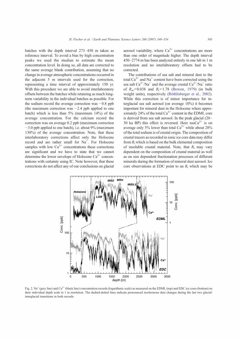
batches with the depth interval 273–450 m taken asreference interval. To avoid a bias by high concentrationpeaks we used the median to estimate the meanconcentration level. In doing so, all data are corrected tothe same average blank contribution, assuming that nochange in average atmospheric concentrations occurred inthe adjacent 5 m intervals used for the correction,representing a time interval of approximately 150 yr.With this procedure we are able to avoid interlaboratoryoffsets between the batches while retaining as much long-term variability in the individual batches as possible. Forthe sodium record the average correction was −0.8 ppb(the maximum correction was −2.4 ppb applied to onebatch) which is less than 5% (maximum 14%) of theaverage concentration. For the calcium record thecorrection was on average 0.2 ppb (maximum correction−3.0 ppb applied to one batch), i.e. about 9% (maximum130%) of the average concentration. Note, that theseinterlaboratory corrections affect only the Holocenerecord and are rather small for Na+. For Holocenesamples with low Ca2+ concentrations these correctionsare significant and we have to state that we cannotdetermine the lower envelope of Holocene Ca2+ concen-trations with certainty using IC. Note however, that thesecorrections do not affect any of our conclusions on glacial
aerosol variability, where Ca2+ concentrations are morethan one order of magnitude higher. The depth interval450–2774 m has been analyzed entirely in one lab in 1 mresolution and no interlaboratory offsets had to becorrected.
The contributions of sea salt and mineral dust to thetotal Ca2+ and Na+ content have been corrected using thesea salt Ca2+/Na+ and the average crustal Ca2+/Na+ ratioof Rm=0.038 and Rt =1.78 (Bowen, 1979) (in bulkweight units), respectively (Röthlisberger et al., 2002).While this correction is of minor importance for in-terglacial sea salt aerosol (on average 10%) it becomesimportant for mineral dust in the Holocene where appro-ximately 24% of the total Ca2+ content in the EDML coreis derived from sea salt aerosol. In the peak glacial (20–30 ka BP) this effect is reversed. Here nssCa2+ is onaverage only 5% lower than total Ca2+ while about 28%of the total sodium is of crustal origin. The composition ofcrustal tracers as recorded in ionic ice core data may differfromRt which is based on the bulk elemental compositionof insoluble crustal material. Note, that Rt may varydependent on the composition of crustal material as wellas on size dependent fractionation processes of differentminerals during the formation of mineral dust aerosol. Icecore observations at EDC point to an Rt which may be
Fig. 2. Na+ (grey line) and Ca2+ (black line) concentration records (logarithmic scale) as measured on the EDML (top) and EDC ice cores (bottom) ontheir individual depth scale in 1 m resolution. The dashed-dotted lines indicate pronounced isochronous dust changes during the last two glacial/interglacial transitions in both records.
343H. Fischer et al. / Earth and Planetary Science Letters 260 (2007) 340–354

closer to 1 (Bigler et al., 2006). While the effect of such avariability in Rt changes the nssCa
2+ estimate only by afew percent, its effect on ssNa+ is considerable. Forinstance reducing Rt within reasonable bounds to 1(Bigler et al., 2006) or increasing it to 3.5 changes thessNa+ estimate by 10–30% for glacial conditions inAntarctica (Fischer et al., 2007). Note, that Rt may alsochange from glacials to interglacials due to potentiallyshifting sources and weathering conditions, however,within reasonable limits of Rt this effect is too small tosignificantly affect our conclusions.
2.3. Accumulation rates and deposition fluxes
The total average deposition flux Jtot at an ice coresite (Fischer et al., 2007) can be approximated by
Jtot ¼ CiceA ¼ vdryCair þW=qairCairA:
The first term on the right hand side of this equationparameterizes the dry deposition and the second term thewet deposition flux with vdry the total mean drydeposition velocity, W the scavenging ratio, ρair thedensity of air, Cair the atmospheric aerosol concentrationand A the average accumulation rate. In low accumu-lation areas dry deposition dominates and the total fluxis essentially independent of changes in accumulationand almost proportional to the atmospheric aerosolconcentrations. Accordingly, we will discuss aerosolflux records in this study, which are more representativeof atmospheric aerosol concentrations. Knowledge ofthe latter is a prerequisite for quantitative estimates ofsource strength or transport changes in the past. Thetotal deposition flux was calculated by multiplying themeasured ice concentration Cice with reconstructedaccumulation rates (Figs. 2 and 3). Both at EDC andEDML the accumulation rate is estimated from the
Fig. 3. Sea salt Na+ (ssNa+) and non-sea salt Ca2+ (nssCa2+) flux records (logarithmic scale) over the last 150 kyr at EDML and EDC on the commonEDML1/EDC3 age scale (Parrenin et al., 2007; Ruth et al., 2007). For comparison past accumulation rates at the site of deposition are given asderived from isotope temperature changes (δ18O, δD) at EDML and EDC (EPICA community members, 2004, 2006) which have been used for fluxcalculations. Data are shown in 1 m resolution (thin grey lines) and 500 yr averages (thick black line for EDML and thin black line for EDC), the latteraccounting for the loss in temporal resolution down core. Also depicted are reconstructed changes in benthic δ18O representative of long-term sealevel changes on the new EDML1/EDC age scale (Bintanja et al., 2005).
344 H. Fischer et al. / Earth and Planetary Science Letters 260 (2007) 340–354
stable water isotope (δ18O, δD) profiles (after correctionfor changes in the isotopic composition of sea water dueto continental ice mass changes) essentially assumingthermodynamic control of the water vapor saturationpressure (EPICA community members, 2006; Parreninet al., 2007). Second order corrections of non-thermo-dynamic effects on the accumulation rate at EDML havebeen made using the spatial variability in accumulationrates upstream of the drill site (EPICA communitymembers, 2006) derived from firn cores and an extendedsurface radar survey (Oerter et al., 2000; Steinhage et al.,2001; Graf et al., 2002; Rybak et al., 2005) and at EDCby a one-dimensional flow model (Parrenin et al., 2007).The error of the reconstructed accumulation rates isestimated to be 30% for glacial times and significantlyless for warm periods, where the precipitation regime issimilar to today. This is also supported by comparingthese continuous thermodynamically derived accumu-lation rates at EDML with discrete accumulation ratesderived from the unstrained layer thickness betweenvolcanic match points (Severi et al., 2007). Bothaccumulation estimates agree typically within ±20%.Because the accumulation information based on δ18Ocan be calculated continuously in high resolution overthe entire length of the core, we will use the thermo-dynamically derived accumulation rate in the followingto derive aerosol fluxes. Based on the errors inaccumulation rates and ion concentrations, the aerosolfluxes are constrained to better than 30% for the largemajority of the samples and to better than 60% for verylow Holocene Ca2+ concentrations. Note, that althoughthese errors are considerable they are small comparedto the order of magnitude change in glacial/interglacialCa2+ concentrations and cannot explain systematicglacial variations on millennial time scales in concen-tration and flux records.
2.4. Upstream correction
In contrast to the EDC ice core, which is located on adome position, the EDML ice core lies at a saddleposition of the ice divide with small (about 1 m/yr)horizontal flow velocities. Accordingly, while the ice atDome C originates at the current drill site, deeper ice atEDML originates from upstream positions at higheraltitudes, where temperatures and accumulation rates arelower and the atmospheric aerosol concentrations maybe slightly different. E.g. ice with an age of 150 ka BPhas been deposited 160 km upstream (EPICA commu-nity members, 2006; Huybrechts et al., 2007). Note, thatgeographic effects in aerosol concentrations are smallcompared to the glacial/interglacial changes (Sommer
et al., 2000; Göktas et al., 2002). As outlined above thetrue total aerosol flux at the site of deposition should bealmost independent from the local snow accumulationrate in low accumulation areas where dry depositionprevails. Accordingly, we used the local accumulationrate at the site of initial deposition to calculate totalaerosol fluxes.
3. Results
The Ca2+ and Na+ concentration records for both icecores are shown on a depth scale in Fig. 2. The EDCrecord provides unprecedented data over 8 full glacialcycles, while the EDML record shows only 2 unam-biguous glacial maxima. In return, the EDML recordexhibits higher annual layer thicknesses down to a depthof 1900 m, allowing for higher resolution records downto an age of approximately 80 ka BP. The concentrationrecords show comparable glacial/interglacial variationsboth at EDML and EDC with 1–2 orders of magnitudehigher sea salt and mineral dust concentrations duringglacial periods and significant millennial dust variabilityduring marine isotope stage 2–4. Similar glacial/interglacial variability has been also reported fromVostok (de Angelis et al., 1997) and Taylor Dome(Mayewski et al., 1996) as far as temporal resolutionallowed.
One major achievement for the EPICA ice cores is theunambiguous stratigraphic link between the two EPICAice cores (Ruth et al., 2007; Severi et al., 2007). Thiscommon EDML1/EDC3 age scale allows for directcomparison of aerosol flux records and their interpretationin terms of atmospheric aerosol concentrations. In Fig. 3the ssNa+ and nssCa2+ flux records are plotted. Theaccompanying changes in the snow accumulation rate aregiven for comparison. Clearly, both records show a veryhigh covariance between both sites in each of the aerosolspecies. However, nssCa2+ fluxes at EDML are about 3times higher than at EDC showing that atmosphericnssCa2+ concentrations are substantially higher at EDMLthan at EDC. Isotopic fingerprinting for Dome C samplesshowed that Patagonia is the dominant source of mineraldust deposited at that site in the glacial (Basile et al., 1997;Delmonte et al., 2007) as also supported by dust modeling(Lunt and Valdes, 2001; Mahowald et al., 2006). In theinterglacial an additional Australian dust source may bepossible at Dome C (Revel-Rolland et al., 2006;Delmonte et al., 2007). Isotopic fingerprinting of mineraldust has not been accomplished yet at EDML, but a stronginfluence of Australian dust sources to EDML appears tobe very unlikely, given its geographic location which ismuch closer to South America and downwind of the
345H. Fischer et al. / Earth and Planetary Science Letters 260 (2007) 340–354

cyclonically curved atmospheric pathway from Patagonia(Reijmer et al., 2002). Accordingly, we attribute thehigher atmospheric nssCa2+ concentrations at EDML tothe greater proximity of EDML to the Patagonian dustsource.
Also sea salt fluxes are about a factor of 2 higher atEDML than at EDC indicating higher atmospheric seasalt aerosol concentrations in Dronning Maud Land.Note, that in the case of sea salt wet deposition may havea stronger influence than is the case for dust. Transport ofsea salt aerosol is closely linked to cyclonic activity and ahigher contribution by wet deposition of sea salt aerosolmay be expected. This holds especially at EDML, wherelarge parts of the recent annual accumulation is derivedfrom a few single snow fall events per year (Reijmer andvan den Broeke, 2001), while at EDC only non-frontaldiamond dust is observed. Model studies show thatcircum-Antarctic cyclone activity in the glacial was mostlikely reduced (Krinner and Genthon, 1998) due to theextended sea ice cover and an accompanying northwardshift of the atmospheric polar front, reducing the effect ofsingle precipitation events on sea salt transport to EDMLat that time. Given the high covariance between bothrecords and the extremely low glacial accumulation of1–3 cm WE/yr at both sites a dominant influence of wetdeposition during cold climate periods appears to beunlikely. This implies that glacial sea salt fluxes arelargely representative of the true variations in atmo-spheric concentrations.
Most striking are the substantial changes in dust andsea salt fluxes over the last glacial cycle similarly foundat both sites. The nssCa2+ flux decreased by a factor ofabout 10 during the last two glacial/interglacial transi-tions (Fig. 3) at both sites. At the same time the ssNa+
flux decreased at EDC by a factor of 2 and at EDML by afactor of 3 from the Last Glacial Maximum (LGM) to theHolocene and by a factor of 4–8 during the penultimatetransition, essentially due to much lower ssNa+ fluxesduring the interglacial MIS 5.5. Apart from the glacial/interglacial changes in dust emissions, strong millennialvariations in the nssCa2+ flux are also observed, whilesuch variations are very subdued in the sea salt record.
4. Discussion
4.1. Mineral dust
A key question is, how much of the glacial/interglacialandmillennial variations in the glacial is due to changes inthe aerosol transport or changes in aerosol source strength.Using the coherent change in glacial dust fluxes at bothEPICA sites from opposite sides of the East Antarctic
plateau (r2=0.82 for 100 yr averages), we are now able toconstrain the influence of transport changes on thechanges in mineral dust flux in Antarctica. Assumingthe atmospheric aerosol concentration close to the sourceis given by Cair(0) and an air parcel is transported awayfrom the source, the atmospheric aerosol concentrationCair at any time t along the transport trajectory can to firstorder be approximated by
CairðtÞ ¼ Cairð0Þexpð�t=sÞ or
log½CairðtÞ=Cairð0Þ� ¼ �t=s
where t is the transport time and the average atmosphericresidence time τ along the transport route is controlled bywet and dry deposition (Hansson, 1994). τ is typically onthe order of a few days to weeks (Mahowald et al., 1999;Gong et al., 2002; Reijmer et al., 2002; Werner et al.,2002). If two sites with transport times t1 and t2 (e.g.EDML and EDC) are considered, the logarithmic airconcentration at site 2 can be expressed by the con-centration at site 1 according to
log½Cairðt2Þ� ¼ log½Cairðt1Þ� � Dt=s ð1ÞwhereΔt= t2− t1 is the transport time difference along thetwo trajectories andwhere we assume that the atmosphericresidence time along both transport routes is comparable.
Fig. 4. Scatter plot of logarithmic nssCa2+ (light grey dots) and ssNa+
(dark grey dots) fluxes in the EDC vs. EDML ice cores in 100 yrresolution according to Eq. (1). If transport remains unchanged thedifference of the data points from the first bisecting line should stayconstant. For visual guidance a linear regression through all data pointshas been added which shows a slope close to 1 for nssCa2+ (dark greyline) and around 0.6 for ssNa+ (light grey line).
346 H. Fischer et al. / Earth and Planetary Science Letters 260 (2007) 340–354

Accordingly, if the aerosol is derived from the same sourceat both sites (as is the case for glacial Patagonian dust inAntarctica) the difference in the logarithmic atmosphericaerosol concentration (thus, the deposition flux inAntarctic low accumulation areas), should be Δt/τ. Theoffset Δt/τ may change for different climate conditions.For example if transport velocities intensify as hypothe-sized for colder climate conditions (Petit et al., 1999), Δtand, thus, the logarithmic offset should become smaller. Ifthe atmospheric residence time τ is considerably length-ened as hypothesized for cold periods (Yung et al., 1996;Petit et al., 1999) the offset should also be reduced.
As shown in Fig. 4 the difference of logarithmicnssCa2+ fluxes in the ice (representative of atmosphericnssCa2+ concentrations) at EDC and EDML stayed ratherconstant, providing observational evidence that transportparameters for dust transport fromPatagonia toAntarcticahave not changed strongly over the last glacial cycles.Alternatively, both Δt and τ may have changed in thesame way compensating each other's transport effect.However, it seems unlikely that this was the case duringall time periods over the last 150 kyr. In any case thechange in atmospheric concentration at the drill site isonly dependent on the joint effect of transport time andresidence timewhich, based on our results, was limited. InTable 1 the average differences (representative ofΔt/τ) oflogarithmic fluxes between EDML and EDC aresummarized for individual time periods. Based on ourconceptual model it becomes clear that Δt/τ is between 1and 2 for all time periods over the last glacial cycle,implying that the difference in transport time is similar tothe atmospheric residence time and is on the order of aweek approximately in line with back trajectory studies(Reijmer et al., 2002). For the glacial intervals, wherePatagonian dust is dominant (Grousset et al., 1992; Basileet al., 1997; Delmonte et al., 2004a), the offset liesbetween 1 and 1.5 with the lower values for peak glacialconditions (LGM, MIS6). This points to a somewhatfaster transport or a larger residence time during thecoldest periods but the decrease inΔt/τ fromMIS3 to theLGM is still within the uncertainty in Table 1. Taking thevalues in Table 1 at face value a LGM decrease in Δt/τ
compared to MIS3 could explain increases in theatmospheric nssCa2+ concentration of approximately40% assuming that this change were entirely due tochanges in atmospheric residence time and if we assumeboth an average atmospheric residence time and a trans-port time to EDML of approximately a week during MIS3 (Gong et al., 2002). Only if we use an unrealisticallylong transport time, which is 6 times larger than theatmospheric residence time, can we explain the observedfactor of 5 changes in the glacial nssCa2+ flux recordswithour simple conceptual transport model. The largestdifference in Table 1 is found between the Holoceneand the LGM. Taken at face value this would point to aslower transport or a reduced atmospheric residence timeduring the Holocene, which could explain a glacialincrease by 70%. However, the Holocene Ca2+ flux atEDML has to be regarded as an upper limit due to therelatively high blank contribution in this time interval andaccordingly the real difference in Δt/τ in Table 1 issignificantly smaller. E.g. reducing the average Holoceneconcentration at EDML for a blank contribution of only1 ppb would reduce Δt/τ to 1.5, i.e. a value similar toMIS3 and 4.
Interestingly, the scatter of the nssCa2+ flux data inFig. 4 decreases with increasing flux values, i.e. for colderclimate conditions. This can only partly be explained bythe larger measurement uncertainty for low Ca2+
concentrations during warm periods. Accordingly, thissuggests a higher transport variability or a variable input ofAustralian dust export to Antarctica for warm climateconditions. In summary, we conclude that both transportintensity as well as variability changed over time butplayed only a secondary role for the observed dust changesin line with atmospheric circulation models (Krinner andGenthon, 1998; Reader and McFarlane, 2003; Mahowaldet al., 2006). Thus, the observed changes in nssCa2+ fluxespredominantly reflect changes in source strength.
For glacial dust this implies strongly increased dustemissions in Patagonia, which are most pronouncedduring the LGM. The penultimate glacial but also thecold interval between 60–70 ka BP show extraordinarilyhigh nssCa2+ fluxes comparable to the environmental
Table 1Average±standard deviation of the difference in logarithmic nssCa2+ fluxes in 100 yr resolution at EDML and EDC representing the average ratio ofthe transport time difference between the two sites and the atmospheric residence time as controlled by wet and dry deposition en route
Timeperiod
Holocene LGM MIS3 MIS4-5.4 MIS5.5 MIS6
1–10 ka BP 20–30 ka BP 30–60 ka BP 60–120 ka BP 120–130 ka BP 130–150 ka BP
Δt/τ (2.01±0.47) 0.96±0.17 1.41±0.40 1.56±0.84 (1.45±0.51) 1.16±0.39
The Holocene value represents an upper limit due to the larger blank contribution to ion chromatographically determined Ca2+ concentrations atEDML compared to the CFA data used at EDC. During MIS5.5 both EDML and EDC are affected by the blank level.
347H. Fischer et al. / Earth and Planetary Science Letters 260 (2007) 340–354

conditions during the LGM. Parallel to the nssCa2+ fluxmaxima in Antarctica, terrigenous records in marinesediments in the northern Scotia Sea also point to highermineral dust input from southern Patagonian sources(Diekmann et al., 2000), however this study did notdistinguish between aeolian and lateral transport ofsuspended particles to the sediment. The rest of the lastglacial is characterized by intermediate nssCa2+ fluxes,hence mineral dust emissions in Patagonia, which arestrongly but not linearly related to temperature changesrecorded in Antarctica (Fig. 5) (Wolff et al., 2006).Especially, each of the Antarctic Isotope Maxima (AIM)(EPICA community members, 2006) indicated in Fig. 3is accompanied by a significant decline in nssCa2+ fluxesat EDML and EDC. This points to synchronous changes(reduced aridity and/or lower wind speeds) in the Pata-gonian source regions during AIMs. Of special impor-tance in Fig. 3 are also the apparently comparableenvironmental conditions during the last two intergla-cials. This points to similar precipitation rates and windspeeds in Patagonia while temperatures in Antarcticawere 2–4 °C higher in MIS5.5 than in the Holocene(EPICA community members, 2006).
Little is known about the long-term change in localPatagonian climate beyond the LGM. For the LGM,terrestrial records ((Markgraf et al., 1992) and referencestherein) and climate models (Wainer et al., 2005) suggestincreased aridity leeside of the Andes and a northwardexpansion and potential strengthening of the westerlies(Moreno et al., 1999). The latter is connected to the
northward expansion of sea ice found inmarine sedimentrecords (Gersonde et al., 2005) and in line with our seasalt reconstructions discussed in Section 4.2. Modelsimulations on the change in the southern hemispherewesterlies are inconsistent (Shin et al., 2003; Butzinet al., 2005; Otto-Bliesner et al., 2006). While anidealized atmospheric model without continents shows aclear glacial northward shift of peak westerly winds(Williams and Bryan, 2006), one model study with acomplex coupled ocean/atmosphere climate model (Shinet al., 2003) shows even a slight southward shift of thepeak wind stress in the SO. Interestingly, a northwardexpansion of the westerlies is also observed for recentwinter conditions compared to summer in NCEP/NCARreanalysis data (Kalnay et al., 1996), while the core of thewesterlies in the SO does not shift in latitude.
Another possible factor acting on dust emission maybe the reduction of sea level exposing substantial shelfareas especially on the Atlantic side off Patagonia.Comparison of the EDC nssCa2+ record with coast linereconstructions for the Argentinian shelf (Wolff et al.,2006) showed that the major glacial/interglacial nssCa2+
decrease occurred prior to any significant sea level rise.In addition the millennial climate variability during MIS3 is also accompanied by significant nssCa2+ fluxvariations (Fig. 3), but has not been accompanied by sealevel changes at similar high frequencies. In contrast tothe delayed global sea level rise relative to the mineraldust decrease, an early glacier retreat before 17 ka BPhas been reported from Tierra del Fuego and other mid-
Fig. 5. Temperature dependence of nssCa2+ (left) and ssNa+ (right) fluxes in 500 yr resolution at EDML (dark grey dots) and EDC (light grey dots).Surface temperatures have been derived from δ18O (EDML) and δD (EDC) using the spatial isotope/temperature gradient in the respective region(EPICA community members, 2004, 2006).
348 H. Fischer et al. / Earth and Planetary Science Letters 260 (2007) 340–354

latitude glaciers (Sugden et al., 2005; Schaefer et al.,2006), supporting a close connection of glaciation andcontinental dust sources in southern South America.Outwash of mineral dust material has been stronglyenhanced during glacial expansion of southern Andeanice masses, providing a potential active source formineral dust mobilization in the glacial. In summary wesuggest that a combination of changes in glacialoutwash, aridity and wind speed are mainly responsiblefor the glacial/interglacial mineral dust changesrecorded in Antarctica (Mahowald et al., 2006) whilethe influence of sea level changes is small for the rapiddecrease in dust fluxes at the beginning of the ter-mination and during MIS 3.
4.2. Sea salt
A quantification of transport changes for sea saltaerosol is even more difficult as in the case of dust. Seasalt concentration increases more strongly at EDMLthan at EDC for colder climate conditions leading to anincrease in the difference of logarithmic sea saltconcentration in Fig. 4. However, this cannot be usedto quantify transport changes as in the case of glacialdust because the sea salt source regions for the Atlanticand Indian Ocean sector of Antarctica are not the sameand sea salt source strength as well as transport mayhave changed independently in both regions. In view ofthe largely expanded sea ice coverage around Antarcticaa longer transport time from the open ocean to theAntarctic plateau is expected in glacial periods and anyintensification of transport from the open ocean wouldhave to overcompensate that effect. An increased inflowof marine air masses from the open ocean leading to anincreased sea salt aerosol flux seems also in contradic-tion with the strongly depleted stable water isotope(δ18O, δD) levels (EPICA community members, 2004,2006) and reduced snow accumulation rates at bothsites, pointing to a stronger depletion of marine air mas-ses in water vapor and most likely also sea salt aerosolduring transport.
Also an explanation of the site dependent glacialincrease in sea salt fluxes in terms of sea salt sourcestrength is not straightforward. The canonical interpre-tation of changes in sea salt aerosol is an increased sea/airparticle flux at the open ocean surface due to increasedwind speeds. This, however, is in contradiction to thegreatly increased sea ice cover (Gersonde et al., 2005)during glacial periods. Aerosol formation from brinewater, as for example experienced during the formationof frost flowers in sea ice leads and polynyas, hasrecently been identified as an additional effective source
for sea salt aerosol (further on referred to as “sea icesalt”). Precipitation of mirabilite (Na2SO4·10H2O) fromsea water during brine formation leads to a characteristicsulfate depletion compared to the average sea watercomposition. This fractionation has been regularlyobserved in atmospheric sea salt aerosol concentrationsat coastal Antarctic sites in winter (Wagenbach et al.,1998; Rankin et al., 2000) showing the importance of thebrine water source for the local sea salt aerosol budget.Brine and frost flower formation was also suggested as apossible mechanism for the glacial/interglacial increasein sea salt concentrations in ice cores on the highAntarctic plateau (Wolff et al., 2003, 2006). Only recent-ly, year-round aerosol sampling on the East Antarcticplateau revealed evidence of sulfate depleted sea saltaerosol during austral winter (Hara et al., 2004), whichwe interpret as significant influence of sea ice formationon the sea salt aerosol budget also for the interior ofAntarctica (Wolff et al., 2006; Fischer et al., 2007). In thefollowing we will explore whether we can explain theobserved changes in sea salt fluxes, if we take sea ice saltformation into account, while recognizing that thereremains some controversy about this interpretation aslong as we have no quantitative source estimate for seaice salt production.
Due to wind driven opening of leads this sea ice saltaerosol formation process occurs throughout the sea icecover and continuously in coastal polynyas. Based ondiatom evidence in SO sediment records it was shownthat the circum-Antarctic winter sea ice cover during theLGM was enhanced by approximately a factor of twofrom 19 to 39 ·106 km2 (Gersonde et al., 2005). Al-though the reconstruction of the summer sea ice edge ishampered by the lack of siliceous sediments in regionsof second year sea ice, some evidence for substantialsummer sea ice exists for the LGM in the Atlantic andIndian Ocean sector of the SO (Gersonde et al., 2005).This indicates that the glacial summer sea ice was aslarge as recent winter sea ice coverage in the Atlanticsector while it was not extended in the Indian Oceansector of the SO. Sea surface temperatures in summersea ice regions (e.g. in coastal polynyas in the WeddellSea) have been well below the freezing point during theLGM (Gersonde et al., 2005), allowing for considerablesea ice formation also during summer. This summer seaice salt formation would add to the sea ice salt aerosolemission in winter and further enhance the annuallyaveraged aerosol source strength of this process. If wetake at first order the sea ice salt contribution to theAntarctic sea salt budget to be proportional to the totalsea ice cover in winter and summer we expect a factor of2 increase in the Indian ocean and a factor up to 3
349H. Fischer et al. / Earth and Planetary Science Letters 260 (2007) 340–354
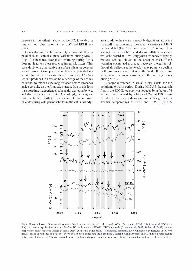
increase in the Atlantic sector of the SO, favorably inline with our observations in the EDC and EDML icecores.
Concentrating on the variability in sea salt flux inparallel to millennial climate variations during MIS 3(Fig. 4) it becomes clear that a warming during AIMsdoes not lead to a clear response in sea salt fluxes. Thiscasts doubt on a quantitative use of sea salt in ice cores assea ice proxy. During peak glacial times the potential seaice salt formation zone extends as far north as 50°S. Seaice salt produced in areas at the outer edge of the sea icecover has to travel a very long distance before it reachesan ice core site on the Antarctic plateau. Due to this longtransport time it experiences substantial depletion by wetand dry deposition en route. Accordingly, we suggestthat the farther north the sea ice salt formation zoneextends during cold periods the less efficient is this edge
area to add to the sea salt aerosol budget at Antarctic icecore drill sites. Looking at the sea salt variations inMIS 3in more detail (Fig. 6) we see that at EDC no imprint onsea salt fluxes can be found during AIMs whatsoeverwhile the record at EDML suggests a tendency to rapidlyreduced sea salt fluxes at the onset of most of thewarming events and a gradual recovery thereafter. Al-though this effect is rather weak it may point to a declinein the summer sea ice extent in the Weddell Sea sectorwhich may react more sensitively to the warming eventsduring MIS 3.
A major difference in ssNa+ fluxes exists for thepenultimate warm period. During MIS 5.5 the sea saltflux in the EDML ice core was reduced by a factor of 4while it was lowered by a factor of 2–3 at EDC com-pared to Holocene conditions in line with significantlywarmer temperatures at EDC and EDML (EPICA
Fig. 6. High-resolution (100 yr averages) plots of stable water isotopes, ssNa+ fluxes and nssCa2+ fluxes in the EDML (black line) and EDC (greyline) ice cores during the time interval 22–42 ka BP on the common EDML1/EDC3 age scale (Parrenin et al., 2007; Ruth et al., 2007). Isotopetemperatures show Antarctic Isotope Maxima (AIM) during this period (EPICA community members, 2006) which are also reflected in lowerednssCa2+ fluxes at both sites (indicated by arrows in the bottom panel, note the logarithmic y-scale). Sea salt aerosol at EDML tends to a rapid declineat the onset of most of the AIMs (indicated by arrows in the middle panel) while no significant changes in sea salt aerosol can be observed at EDC.
350 H. Fischer et al. / Earth and Planetary Science Letters 260 (2007) 340–354

community members, 2006). Because summer sea ice isnearly absent in the Indian Ocean sector for Holoceneconditions, this implies that only a reduction in thewinter sea ice salt source could explain the sea saltdecrease in this region during the warmer MIS 5.5. Inthe Atlantic sector of the SO an even stronger decline insea ice coverage during MIS 5.5 is indicated by ourssNa+ data, possibly related to a reduction of both winterand summer sea ice in the Weddell Sea. This is alsosupported by changes in marine sediments, indicating asouthward shift of the opal deposition belt by 3–5°latitude (Bianchi and Gersonde, 2002) at that time.
5. Conclusions
Sea salt and mineral dust aerosol records arerepresentative for basin-wide atmospheric catchmentareas of aerosol transported onto the East Antarctic icesheet. The records allow us to draw a clearer picture on thetiming of environmental changes in Patagonia and the SOand their influence on aerosol formation in parallel toclimate variations in Antarctica over the last 150 kyr.
Sea salt records at both sites allow for the first time abasin-wide estimate of sea salt aerosol emissions, whichsupport an accompanying change in sea ice cover over thecomplete time interval from the penultimate glacial to thepresent. The coherence of the two sea salt records fromopposite sides of the Antarctic ice sheet indicates awaxing and waning of sea ice, which was generally syn-chronous in the Atlantic and the Indian Ocean sector ofthe SO on glacial/interglacial time scales. The sensitivityof sea salt fluxes to temperature changes (Fig. 5),however, is higher in the Weddell Sea sector, a factwhich we attribute to a more vigorous change in sea icecover and the additional role of summer sea ice extent onsea ice salt formation in this area. We note, that for verycold climate conditions sea salt changes become increas-ingly insensitive to temperature changes probably relatedto the long transport distance of aerosol formed at thenorthern margin of the sea ice cover. Accordingly, the useof sea salt as quantitative proxy for sea ice coverage ishampered and requires a rigorous calibration againstmarine sediment data for different time slices, experi-mental studies of the modern sea ice salt source as well asrefined model studies about its change in the past.
Using our dust records from sites facing differentsectors of the SO with greatly different distances toPatagonia and using a simple conceptual transport modelwe can rule out a substantial variation in transport asbeing the main factor being responsible for the observednssCa2+ changes during glacial times as also supportedby atmospheric circulation models (Krinner and Gen-
thon, 1998; Reader and McFarlane, 2003). Instead ourresults point to temporal changes in the strength of thePatagonian mineral dust source in parallel to temperaturevariations in Antarctica. The three times higher nssCa2+
fluxes at EDML also point to a threefold higher aeoliandust input into the Weddell Sea sector of the SO, po-tentially related to a stronger dust fertilization in thisregion. This effect may be amplified by a potential duststorage effect of the greatly extended winter and summersea ice coverage as indicated in our ssNa+ record. Theextension of summer and winter sea ice in this region isalso expected to have a strong effect on bottom waterformation, gas exchange and wind shear of the surfaceocean likely related to a reduced ventilation of the deepSO with strong impacts on the global carbon cycle(Köhler et al., 2005). Accordingly, our data will allow fora better time resolved, basin-wide quantification ofpotential dust fertilization on marine export productivityand investigation of the effect of the sea ice extent on gasexchange and water mass formation.
Acknowledgments
This work is a contribution to the European Project forIce Coring in Antarctica (EPICA), a joint EuropeanScience Foundation/European Commission scientificprogramme, funded by the EU (EPICA-MIS) and by thenational contributions from Belgium, Denmark, France,Germany, Italy, the Netherlands, Norway, Sweden,Switzerland and the United Kingdom. The main logisticsupport was provided by IPEV and PNRA (at Dome C)andAWI (at DronningMaudLand).We thank the logisticsand drilling teams and all helpers in the field for makingthe science possible. This is EPICA publication no. 170.
Appendix A. Supplementary data
Supplementary data associated with this article canbe found, in the online version, at doi:10.1016/j.epsl.2007.06.014.
References
Archer, D., Winguth, A., Lea, D., Mahowald, N., 2001. What causedthe glacial/interglacial atmospheric pCO2 cycles? Rev. Geophys.38, 159–189.
Basile, I., Grousset, F.E., Revel, M., Petit, J.R., Biscaye, P.E., Barkov,N.I., 1997. Patagonian origin of glacial dust deposited in EastAntarctica (Vostok and Dome C) during glacial stages 2, 4 and 6.Earth Planet. Sci. Lett. 146, 573–589.
Bianchi, C., Gersonde, R., 2002. The Southern Ocean surface betweenMarine Isotope Stage 6 and 5d: Shape and timing of climatechanges. Palaeogeogr. Palaeoclimatol. Palaeoecol. 187, 151–177.
351H. Fischer et al. / Earth and Planetary Science Letters 260 (2007) 340–354

Bigler, M., Röthlisberger, R., Lambert, F., Stocker, T.F., Wagenbach,D., 2006. Aerosol deposited in East Antarctica over the last glacialcycle: detailed apportionment of continental and sea salt contribu-tions. J. Geophys. Res. 111. doi:10.1029/2005JD006469.
Bintanja, R., van de Wal, R.S.W., Oerlemans, J., 2005. Modelledatmospheric temperatures and global sea levels over the pastmillion years. Nature 437, 125–128.
Blunier, T., Schwander, J., Stauffer, B., Stocker, T., Dällenbach, A.,Indermühle, A., Tschumi, J., Chappellaz, J., Raynaud, D., Barnola,J.-M., 1997. Timing of the Antarctic Cold Reversal and theatmospheric CO2 increase with respect to the Younger Dryas event.Geophys. Res. Lett. 24, 2683–2686.
Bowen, H.J.M., 1979. Environmental Chemistry of the Elements.Academic Press, London.
Brook, E.J., White, J.W.C., Schilla, A.S.M., M.L.B., Barnett, B.,Severinghaus, J.P., Taylor, K.C., Alley, R.B., Steig, E.J., 2005. Timingof millenial-scale climate change at Siple Dome, West Antarctica,during the last glacial period. Quat. Sci. Rev. 24, 1333–1343.
Butzin, M., Prange, M., Lohmann, G., 2005. Radiocarbon simulationsfor the glacial ocean: the effects of wind stress, Southern Ocean seaice and Heinrich events. Earth Planet. Sci. Lett. 235, 45–61.
de Angelis, M., Steffensen, J.P., Legrand, M., Clausen, H., Hammer,C., 1997. Primary aerosol (sea salt and soil dust) deposited inGreenland ice during the last climatic cycle: comparison with eastAntarctic records. J. Geophys. Res. 102, 26681–26698.
Delmonte, B., Petit, J.R., Maggi, V., 2002. Glacial to Holoceneimplications of the new 27000-year dust record from the EPICADome C (East Antarctica) ice core. Clim. Dyn. 18, 647–660.
Delmonte, B., Basile-Doelsch, I., Petit, J.R., Maggi, V., Revel-Rolland, M., Michard, A., E.J., Grousset, F., 2004a. Comparing theEPICA and Vostok dust records during the last 220,000 years:stratigraphical correlation and provenance in glacial periods.Earth-Sci. Rev. 66, 63–87.
Delmonte, B., Petit, J.R., Andersen, K.K., Basile-Doelsch, I., Maggi,V., Lipenkov, V., 2004b. Dust size evidence for opposite regionalatmospheric circulation changes over East Antarctica during thelast climatic transition. Clim. Dyn. 23, 427–438.
Delmonte, B., Petit, J.R., Basile-Doelsch, I., Jagoutz, E., Maggi, V.,2007. Late Quaternary Interglacials in East Antarctica from ice coredust records. In: Sirocko, F., Claussen, M., Sanchez-Goni, M.F.,Litt, T. (Eds.), The Clim. Past interglacials. Elsevier, Amsterdam,pp. 53–73.
Diekmann, B., Kuhn, G., Rachold, V., Abelmann, A., Brathauer, U.,Fütterer, D.K., Gersonde, R., Grobe, H., 2000. Terrigenoussediment supply in the Scotia Sea (Southern Ocean): response tolate Quaternary ice dynamics in Patagonia and on the AntarcticPeninsula. Palaeogeogr. Palaeoclimatol. Palaeoecol. 162, 357–387.
EPICA community members, 2004. Eight glacial cycles from anAntarctic ice core. Nature 429, 623–628.
EPICA community members, 2006. One-to-one coupling of glacialclimate variability in Greenland and Antarctica. Nature 444,195–198.
Fischer, H., Siggaard-Andersen, M.-L., Ruth, U., Röthlisberger, R.,Wolff, E., 2007. Glacial/interglacial changes in mineral dust andsea salt records in polar ice cores: sources, transport, deposition.Rev. Geophys. 45. doi:10.1029/2005RG000192.
Gersonde, R., Crosta, X., Abelmann, A., Armand, L., 2005. Sea-surfacetemperature and sea ice distribution of the Southern Ocean at theEPILOG Last Glacial Maximum — a circum-Antarctic view basedon siliceous microfossil records. Quat. Sci. Rev. 24, 869–896.
Göktas, F., Fischer, H., Oerter, H., Weller, R., Sommer, S., Miller, H.,2002. A glacio-chemical characterisation of the new EPICA deep
drilling site on Amundsenisen, Dronning Maud Land, Antarctica.Ann. Glaciol. 35, 347–354.
Gong, S.L., Barrie, L.A., Lazare, M., 2002. Canadian Aerosol Module(CAM): a size segregated simulation of atmospheric aerosolprocesses for climate and air quality models 2. Global sea-salt aerosoland its budgets. J. Geophys. Res. 107. doi:10.1029/2001JD002004.
Graf, W., Oerter, H., Reinwarth, O., Stichler, W., Wilhelms, F., Miller,H., Mulvaney, R., 2002. Stable isotope records from DronningMaud Land, Antarctica. Ann. Glaciol. 35, 195–201.
Grousset, F.E., Biscaye, P.E., Revel, M., Petit, J.-R., Pye, K.,Joussaume, S., Jouzel, J., 1992. Antarctic (Dome C) ice coredust at 18 k.y. B.P.: isotopic constraints on origins. Earth Planet.Sci. Lett. 111, 175–182.
Hansson, M.E., 1994. The Renland ice core. A Northern Hemisphererecord of aerosol composition over 120000 years. Tellus 46,390–418.
Hara, K., Osada, K., Kido, M., Hayashi, M., Matsunaga, K., Iwasaka,Y., Yamanouchi, T., Hashida, G., Fukatsu, T., 2004. Chemistry ofsea-salt particles and inorganic halogen species in Antarcticregions: compositional differences between coastal and inlandstations. J. Geophys. Res. 109. doi:10.1029/2004JD004713.
Huybrechts, P., Rybak, O., Pattyn, F., Ruth, U., Steinhage, D., 2007.Ice thinning, upstream advection, and non-climatic biases for theupper 89% of the EDML ice core from a nested model of theAntarctic ice sheet. Clim. Past Disc. 3, 693–727.
Jouzel, J., Masson-Delmotte, V., Cattani, O., Dreyfus, G., Falourd, S.,Hoffmann, G., Minster, B., Nouet, J., Barnola, J.-M., Chappellaz, J.,Fischer, H., Gallet, J.C., Johnsen, S., Leuenberger,M., Loulergue, L.,Luethi, D., Oerter, H., Parrenin, F., Raisbeck, G., Raynaud, D.,Schwander, J., Spahni, R., Souchez, R., Selmo, E., Schilt, A.,Steffensen, J.P., Stenni, B., Stauffer, B., Stocker, T.F., Tison, J.-L.,Werner, M., Wolff, E.W., in press. Orbital and millennial Antarcticclimate variability over the last 800 000 years. Science.
Kalnay, E., Kanamitsu, M., Kistler, R., Collins, W., Deaven, D.,Gandin, L., Iredell, M., Saha, S., White, G., Woollen, J., Zhu, Y.,Chelliah, M., Ebisuzaki, W., Higgins, W., Janowiak, J., Mo, K.C.,Ropelewski, C., Wang, J., Leetmaa, A., Reynolds, R., Jenne, R.,Joseph, D., 1996. The NCEP/NCAR 40-year reanalysis project.Bull. Am. Meteorol. Soc. 77, 437–471.
Knorr, G., Lohmann, G., 2003. Southern Ocean origin for the resump-tion of Atlantic thermohaline circulation during deglaciation.Nature 424, 532–536.
Köhler, P., Fischer, H., Munhoven, G., Zeebe, R.E., 2005. Quantita-tive interpretation of atmospheric carbon records over the lastglacial termination. Glob. Biogeochem. Cycles 19. doi:10.1029/2004GB002345.
Krinner, G., Genthon, C., 1998. GCM simulation of the Last GlacialMaximum surface climate of Greenland and Antarctica. Clim.Dyn. 14, 741–758.
Lunt, D.J., Valdes, P.J., 2001. Dust transport to Dome C, Antarctica, atthe Last Glacial Maximum and present day. Geophys. Res. Lett.28, 295–298.
Mahowald, N., Kohfeld, K., Hansson,M., Balkanski, Y., Harrison, S.P.,Prentice, I.C., Schulz, M., Rodhe, H., 1999. Dust sources anddeposition during the last glacial maximum and current climate: acomparison of model results with paleodata from ice cores andmarine sediments. J. Geophys. Res. 104, 15895–15916.
Mahowald, N.M., Muhs, D.R., Levis, S., Rasch, P.J., Yoshioka, M.,Zender, C.S., Luo, C., 2006. Change in atmospheric mineralaerosols in response to climate: last glacial period, preindustrial,modern, and doubled carbon dioxide climates. J. Geophys. Res.111. doi:10.1029/2005JD006653.
352 H. Fischer et al. / Earth and Planetary Science Letters 260 (2007) 340–354

Markgraf, V., Dodson, J.R., Kershaw, A.P., McGlone, M.S., Nicholls,N., 1992. Evolution of late Pleistocene and Holocene climates inthe circum-South Pacific land areas. Clim. Dyn. 6, 193–211.
Martin, J., 1990. Glacial–interglacial CO2 change: the iron hypothesis.Paleoceanography 5, 1–13.
Mayewski, P.A., Twickler, M.S., Whitlow, S.I., Meeker, L.D., Yang,Q., Thomas, J., Kreutz, K., Grootes, P.M., Morse, D.L., Steig, E.J.,Waddington, E.D., Saltzman, E.S., Whung, P.-Y., Taylor, K.C.,1996. Climate change during the last deglaciation in Antarctica.Science 272, 1636–1638.
Moreno, P.I., Lowell, T.V., Jacobson Jr., G.L., Denton, G.H., 1999.Abrupt vegetation and climate changes during the last glacialmaximum and last termination in the Chilean Lake District. A casestudy from Canal de la Puntilla (41°S). Geogr. Ann. 81A, 285–311.
Morgan, V., Delmotte, M., van Ommen, T., Jouzel, J., Chappellaz, J.,Woon, S., Masson-Delmotte, V., Raynaud, D., 2002. Relativetiming of deglacial climate events in Antarctica and Greenland.Science 297, 1862–1864.
Oerter, H., Wilhelms, F., Jung-Rothenhäusler, F., Göktas, F., Miller,H., Graf, W., Sommer, S., 2000. Accumulation rates in DronningMaud Land, Antarctica, as revealed by dielectric-profilingmeasurements of shallow firn cores. Ann. Glaciol. 30, 27–34.
Otto-Bliesner, B.L., Brady, E.C., Clauzet, G., Tomas, R., Levis, S., Z.K.,2006. Last Glacial Maximum and Holocene climate in CCSM3. J.Clim. 19, 2526–2544.
Parrenin, F., Barnola, J.-M., Beer, J., Blunier, T., Castellano, E.,Chappellaz, J., Dreyfus, G., Fischer, H., Fujita, S., Jouzel, J.,Kawamura, K., Lemieux-Dudon, B., Loulergue, L., Masson-Delmotte, V., Narcisi, B., Petit, J.-R., Raisbeck, G., Raynaud, D.,Ruth, U., Schwander, J., Severi, M., Spahni, R., Steffensen, J.P.,Svensson, A., Udisti, R., Waelbroeck, C., Wolff, E., 2007. TheEDC3 agescale for the EPICA Dome C ice core. Clim. Past Disc.3, 575–606.
Petit, J.R., Mounier, L., Jouzel, J., Korotkevich, Y.S., Kotlyakov, V.,Lorius, C., 1990. Paleoclimatological and chronological implica-tions of the Vostok core dust record. Nature 343, 429–436.
Petit, J.R., Jouzel, J., Raynaud, D., Barkov, N.I., Barnola, J.-M.,Basile, I., Bender, M., Chappellaz, J., Davis, M., Delaygue, G.,Delmotte, M., Kotlyakov, V.M., Legrand, M., Lipenkov, V.Y.,Lorius, C., Pepin, L., Ritz, C., Saltzman, E., Stievenard, M., 1999.Climate and atmospheric history of the past 420,000 years from theVostok ice core, Antarctica. Nature 399, 429–436.
Rankin, A.M., Auld, V., Wolff, E.W., 2000. Frost flowers as a sourceof fractionated sea salt aerosol in the polar regions. Geophys. Res.Lett. 27, 3469–3472.
Reader, M.C., McFarlane, N., 2003. Sea-salt aerosol distributionduring the Last Glacial Maximum and its implications for mineraldust. J. Geophys. Res. 108. doi:10.1029/2002JD002063.
Reijmer, C.H., van den Broeke, M.R., 2001. Moisture sources ofprecipitation inWestern DronningMaud Land, Antarctica. Antarct.Sci. 13, 210–220.
Reijmer, C.H., van den Broeke, M.R., Scheele, M.P., 2002. Air parceltrajectories to five deep drilling locations on Antarctica, based onthe ERA-15 data set. J. Clim. 15, 1957–1968.
Revel-Rolland,M.,DeDekker, P., Delmonte, B., Hesse, P.P.,Magee, J.W.,Basile-Doelsch, I., Grousset, F., Bosch, D., 2006. Eastern Australia: apossible source of dust in East Antarctica interglacial ice. Earth Planet.Sci. Lett. 249, 1–13.
Röthlisberger, R., Bigler, M., Hutterli, M., Sommer, S., Stauffer, B.,Junghans, H.G., Wagenbach, D., 2000. Technique for continuoushigh-resolution analysis of trace substances in firn and ice cores.Environ. Sci. Technol. 34, 338–342.
Röthlisberger, R., Mulvaney, R., Wolff, E.W., Hutterli, M., Bigler, M.,Sommer, S., Jouzel, J., 2002. Dust and sea-salt variability in centralEast Antarctica (Dome C) over the last 45 kyrs and its implicationsfor southern high-latitude climate. Geophys. Res. Lett. 29.doi:10.1029/2002GL015186.
Ruth, U., Barnola, J.-M., Beer, J., Bigler,M., Blunier, T., Castellano, E.,Fischer, H., Fundel, F., Huybrechts, P., Kaufmann, P., Kipfstuhl, S.,Lambrecht, A., Morganti, A., Oerter, H., Parrenin, F., Rybak, O.,Severi, M., Udisti, R., Wilhelms, F., Wolff, E., 2007. “EDML1”: Achronology for the EDML ice core, Antarctica, over the last 150000 year. Clim. Past Disc. 3, 549–574.
Rybak, O., Huybrechts, P., Steinhage, D., Pattyn, F., 2005. Dating andaccumulation rate reconstruction along the Dome Fuji—Kohnenradio-echo-sounding profile. Geophys. Res. Abstr. 7, 05421.
Schaefer, J.M., Denton, G.H., Barrell, D.J.A., Ivy-Ochs, S., Kubik, P.W.,Andersen, B.G., Phillips, F.M., Lowell, T.V., Schlüchter, C., 2006.Near synchronous interhemispheric termination of the Last GlacialMaximum in mid-latitudes. Science 312, 1510–1513.
Severi, M., Castellano, E., Morganti, A., Udisti, R., Ruth, U., Fischer, H.,Huybrechts, P., Wolff, E., Parrenin, F., Kaufmann, P., Lambert, F.,Steffensen, J.P., 2007. Synchronisation of the EDML1 and EDC3timescales for the last 52 kyr by volcanic signature matching. Clim.Past Disc. 3, 409–433.
Shin, S.-I., Liu, Z., Otto-Bliesner, B., Brady, E.C., Kutzbach, J.E.,Harrison, S.P., 2003. A simulation of the Last Glacial Maximumclimate using the NCAR-CCSM. Clim. Dyn. 20, 127–151.
Sommer, S., Wagenbach, D., Mulvaney, R., Fischer, H., 2000. Glacio-chemical study covering the past 2 kyr on three ice cores fromDronning Maud Land, Antarctica 2. Seasonally resolved chemicalrecords. J. Geophys. Res. 105, 29423–29433.
Steig, E.J., Brook, E.J., White, J.W.C., Sucher, C.M., Bender, M.L.,Lehman, S.J., Morse, D.L., Waddington, E.D., Clow, G.D., 1998.Synchronous climate changes in Antarctica and the North Atlantic.Science 282, 92–95.
Steinhage, D., Nixdorf, U., Meyer, U., Miller, H., 2001. Subglacialtopography and internal structure of central and western DronningMaud Land, Antarctica, determined from airborne radio echosounding. J. Appl. Geophys. 47, 183–189.
Stephens, B.B., Keeling, R.F., 2000. The influence of Antarctic sea iceon glacial–interglacial CO2 variations. Nature 404, 171–174.
Stocker, T., Johnsen, S., 2003. A minimum thermodynamic model of thebipolar seesaw. Paleoceanography 18. doi:10.1029/2003PA000920.
Sugden, D.E., Bentley, M.J., Fogwill, C.J., Hulton, N.R.J., McCul-loch, R.D., Purves, R.S., 2005. Late-glacial glacier events insouthernmost South America. Geogr. Ann. 87A, 273–288.
Toggweiler, J.R., 1999. Varition of atmospheric CO2 by ventilation ofthe ocean's deepest water. Paleoceanography 14, 571–588.
Toggweiler, J.R., Russell, J.L., Carson, S.R., 2006. Midlatitudewesterlies, atmospheric CO2, and climate change during the iceages. Paleoceanography 21. doi:10.1029/2005PA001154.
Udisti, R., Becagli, S., Benassai, S., de Angelis, M., Hansson, M.E.,Jouzel, J., Schwander, J., Steffensen, J.P., Traversi, R., Wolff, E.,2004. Sensitivity of chemical species to climatic changes in the last45 kyr as revealed by high-resolution Dome C (East Antarctica)ice-core analysis. Ann. Glaciol. 39, 457–466.
Wagenbach, D., Ducroz, F., Mulvaney, R., Keck, L., Minikin, A.,Legrand, M., Hall, J.S., Wolff, E.W., 1998. Sea-salt aerosol incoastal Antarctic regions. J. Geophys. Res. 103, 10961–10974.
Wainer, I., Clauzet, G., Ledru, M.-P., Brady, E.C., Otto-Bliesner, B.,2005. Last Glacial Maximum in South America: paleoclimateproxies and model results. Geophys. Res. Lett. 32. doi:10.1029/2004GL021244.
353H. Fischer et al. / Earth and Planetary Science Letters 260 (2007) 340–354

Watanabe, O., Jouzel, J., Johnsen, S., Parrenin, F., Shoji, H., Yoshida,N., 2003. Homogeneous climate variability across East Antarcticaover the past three glacial cycles. Nature 422, 509–512.
Werner, M., Tegen, I., Harrison, S.P., Kohfeld, K., Prentice, I.C.,Balkanski, Y., Rodhe, H., Roelandt, C., 2002. Seasonal and inter-annual variability of the mineral dust cycle under present and glacialconditions. J. Geophys. Res. 107. doi:10.1029/2002JD002365.
Williams, G.P., Bryan, K., 2006. Ice age winds: an aquaplanet model.J. Clim. 19, 1706–1715.
Wolff, E.W., Rankin, A.M., Röthlisberger, R., 2003. An ice coreindicator of Antarctic sea ice production? Geophys. Res. Lett. 30.doi:10.1029/2003GL018454.
Wolff, E.W., Fischer, H., Fundel, F., Ruth, U., Twarloh, B., Littot, G.C.,Mulvaney, R., de Angelis, M., Boutron, C.F., Hansson, M., Jonsell,U., Hutterli, M., Bigler, M., Lambert, F., Kaufmann, P., Röthlisber-ger, R., Steffensen, J.P., Siggaard-Andersen, M.-L., Udisti, R.,Becagli, S., Castellano, E., Severi, M., Wagenbach, D., Barbante, C.,Gabrielli, P., Gaspari, V., 2006. Southern Ocean sea ice, DMSproduction and iron flux over the last eight glacial cycles. Nature 440,491–496.
Yung, Y., Lee, T., Wang, C.-H., Shieh, Y.-T., 1996. Dust: a diagnosticof the hydrological cycle during the last glacial maximum. Science271, 962–963.
354 H. Fischer et al. / Earth and Planetary Science Letters 260 (2007) 340–354
Paper III
ICP-Time of Flight-MS as a versatile tool for ultratrace element analysis in Antarctic ice
Dick, D., Wegner, A., Gabrielli, P., Barbante, C., Ruth, U., Kriews,M., to be submitted to Analytical Chimica Acta.

ICP-Time of Flight-MS as a versatile tool for ultra trace element analysis
in Antarctic ice
D. Dick, A. Wegner, P. Gabrielli+,�, C. Barbante+, U. Ruth, M. Kriews*
Alfred Wegener Institute for Polar and Marine Research, Am Handelshafen 12, 27570 Bremerhaven
+Institute for the Dynamics of Environmental Processes – CNR, I-30123 Venice, Italy
�School of Earth Science and Byrd Polar Research Center, Ohio State University,
Columbus, OH 43210-1002, USA
1 Abstract
The importance of trace element analysis in natural samples for climate reconstruction has increased in recent
years. Oftentimes the available sample amount is very restricted. Therefore high sensitive detection systems with
fast data acquisition are required. The inductively coupled plasma time of flight mass spectrometer (ICP-TOF-
MS) meets these demands. Here we present accuracy and precision studies of the ICP-TOF-MS for element
analysis. Therefore reference materials SPS-SW1, SLRS-4 and NIST 1640 were analysed. Further accuracy
studies for rare earth elements (REE) were accomplished with low concentrated molten ice core samples from
Antarctica. Results obtained by ICP-TOF-MS are compared with results obtained by ICP-Quadrupol-MS and
ICP-Sector Field-MS. The presented ICP-TOF-MS correlates very well with ICP-Q-MS and ICP-SF MS as long
as analysed concentrations are higher 4 ng L-1. Below that concentrations the results have to be looked at
carefully.
Keywords: ultra trace element analysis, ICP-TOF-MS, rare earth elements, Antarctic ice
2 Introduction
The earth climate is mainly driven by complex processes between the Arctic and Antarctic. Mineral dust and sea
salt have been deposited on polar ice caps over several thousands of years. Because of the stratigraphic
deposition of snow these chronologically deposited compounds reflect various aspects of climate change [1-4].
Owing to large distances between South America – Antarctica (~1100 km), South Africa – Antarctica (~4000
km) and New Zeeland / Australia Antarctica (~2500 km, ~3000 km), Antarctica is one of the cleanest areas of
the world. Therefore highest demands are posted on sampling of snow and ice cores, sample preparation and
* Correspondance author tel.: +49-(0)471-4831-1420; fax: +49-(0)471-4831-1149; email: [email protected]

finally the analysis of low concentrations [5-7]. The complexity of sampling in the isolated Antarctica implicates
restricted sample volumes available for trace element analysis.
Several methods for trace element analysis in polar snow and ice are performed. Analytical techniques such as
atomic absorption spectrometry (AAS) [8-9], cold vapour atomic fluorescence spectrometry (CVAFS) [10-11]
are used for single element analysis. Isotope dilution mass spectrometry (IDMS) [12] and mass spectrometry
(MS) in general are used for multielement analysis. Information about sea salt, mineral dust and anthropogenic
compounds should be obtained prefereably out of one sample. This is important if high spatial resolution
analysis is accomplished. Thereby, errors generated by assigning the sample to its originating depth are
eliminated. Hence MS is most suitable for multielement analysis.
MS are made up of different components; the mass analyzer determines the type of spectrometer. Sector field
mass spectrometers (SF-MS) [5] and quadrupol mass spectrometers (Q-MS) [7] are the most common MS types
used for investigations of polar ice core samples. These MS measure in the sequential mode. Owing to low
sample volumes a delimited amount of isotopes can be analysed. In contrast to these MS systems the time of
flight-MS (TOF-MS) analyses in the “simultaneous” mode. Major advantages of this system are: no limitations
in the number of analysed isotopes, fast data acquisition and consequently the possibility for numerous replicate
analysis. [13] gives a brief overview on the application of TOF-MS. Until now there is only a spare number of
literature available on the use of TOF-MS for element analysis [14-17] and none publication for element analysis
at the ultra trace concentration level.
The aim of this work is to assess the accuracy and precision of the inductively coupled plasma- TOF-MS (ICP-
TOF-MS) [17-18] developed at the Institute for Analytical Science in Berlin. Therefore reference materials SPS-
SW1, SLRS-4 and NIST 1640 were analysed. Detection limits, the recovery rate and precision, the sample
consumption and analysing time will be presented.
For intercomparison studies natural ice core samples, drilled within the EPICA project (European Project for Ice
Coring in Antarctica) [19] were analysed by ICP-TOF-MS, ICP-Q-MS (Elan 6000, Perkin Elmer/Sciex) and
ICP-SF-MS (Element 2, Thermo Finnigan). Owing to the limitation of analysed isotopes, especially by ICP-SF-
MS, only rare earth element (REE) concentrations are compared. The presented ICP-TOF-MS correlates very
well with ICP-Q-MS and ICP-SF MS as long as analysed concentrations are higher 4 ng L-1. Below that
concentrations the results have to be looked at carefully.

3 Experimental
3.1 Standards and Labware
At the Alfred Wegener Institute (AWI) in Bremerhaven, ultrapure water was produced by coupling a reverse
osmosis system with a Purelab ultra system (Elga, High Wycombe, U.K.). Commercial available ICP-MS
multielement stock solutions (Perkin Elmer) were used for external calibration of the ICP-MS systems. At the
Department of Environmental Science (DES) in Venice, the ultrapure water was produced by coupling a Milli-Q
(Millipore, Bedford, MA) water system with a Purelab Ultra system (Elga, High Wycombe, U.K.). Matrix
matched calibration was done at DES obtained by adding different amounts of multielement standard spikes to a
surface snow sample. At AWI all standards were acidified to pH 1-2 with subboiled HNO3 (distilled 65 %
HNO3, pro analysis, Merck) and contained 1 �g L-1 Rh (RhCl3, Merck) as internal standard. Eppendorf Pipettes
with polypropylene (PP) tips were used for sample and standard preparation. Steps for standard preparation were
done under a clean bench (US Class 100) which was located inside a clean room laboratory, classified as US
Class 10,000, but presently U.S. Class 100-1000 is achieved. At AWI all labware which came into contact with
samples and standards were run through a special cleaning procedure in the following way:
• 1 week treatment with 3 % Mucasol solution (Merck) to degrease all labware, thereafter rinsing all parts with
ultrapure water
• 1 week treatment with 1:4 diluted HCL (30 %, suprapur, Merck) , thereafter rinsing all parts with ultrapure
water
• 1 week treatment with 1:4 diluted HNO3 (distilled 65 %, p.a., Merck) , thereafter rinsing all parts with
ultrapure water
• 1 week treatment with 1:10 diluted HNO3 (65 %, suprapur, Merck) , thereafter rinsing all parts with ultrapure
water
• Drying of all parts in a clean room under a clean bench, US Class 100.
• Packing of all parts in 2 polyethylene (PE) bags for storage
3.2 Sample collection and preparation
3.2.1 Reference material
Three reference materials were used to validate the quality of the ICP-TOF-MS as well as the ICP-Q-MS
measurements.
- SPS-SW1: Spectrapure Standards as, Reference Material for measurements of Elements in Surface Waters

- SLRS-4: National Research Council Canada, River Water Reference Materials for Trace Metals
- NIST 1640: National Institute for Standards and Technology, Trace Elements in Natural Water
Due to the expected REE concentrations in Antarctic ice the SPS-SW1 standard was diluted 1:100. REE from La
to Nd in SLRS-4 were analysed out of a 1:10 dilution, all other REE were analysed without any dilution. In
NIST1640 all REE concentrations were analysed using a 1:10 dilution.
3.2.2 Antarctic Ice Core samples
Within the EPICA a 2774.15 m long ice core (diameter: 98 mm) was drilled in a fluid filled hole at Kohnen
station (Dronning Maud Land (DML), Position: 75°00’S, 0°04’E) and a 3189.45 m long (diameter: 98 mm) was
drilled in a fluid filled hole at Dome C station (Position: 75°06’S, 123°21’E) [19-20]. For shipping and handling
the ice cores are cut in 1 m long sections at Kohnen station and 0.55 m long sections at Dome C station. One
section is called bag, they are consecutively numbered. 22 bags were chosen from each ice core for REE
analysis. Bags from Kohnen station cover the time from the last glacial / interglacial transition. The top of the
youngest bag was 5.78 kyr old and the bottom of the oldest ice core was 48.7 kyr old [21]. Instead the transition
between these two stages is not such good represented by Dome C ice core bags. The top of the youngest ice
core bag was 10.5 kyr old and the bottom of the oldest ice core was 21.5 kyr old [22]. During glacial times the
dust transport is expected to be 4 to 7 times higher compared to warm periods [23], which should also be
reflected in REE- and mineral dust components concentrations.
Each bag of an ice core is used for several ice core studies, therefore a section from the inner part of the ice core
was available for REE analysis. From the top of each bag 30 cm long sections were cut by a band saw and used
for further steps. The sample surface was decontaminated in a first step by sawing 1 cm of the surface with a
band saw. The 30 cm long section was divided in three 10 cm long parts. Each part was rinsed with 1 to 2 L
ultrapure water for three times. In consequence of this procedure the weight of each part was reduced by 50 %.
The three 10 cm long parts of each section were placed in pre-cleaned high density polyethylene (HDPE) bottles
and melted at room temperature. Samples were dispersed by pivoting; aliquots were filled in polystyrene (PS)
CC-accuvettes and finally stored at -20 °C.
Under a clean bench (US-Class 100) which was situated in a clean room laboratory (US-Class 10,000) samples
were molten and transferred into pre-cleaned polyfluor alkoxy (PFA) vessels. The CC-accuvettes were rinsed
with 10 ml subboiled HNO3 (1 Mol L-1) and added into the PFA vessels. Diluted samples were contentrated to
0.5 to 2 ml with a pressure digestion system (Druckaufschlusssystem DAS, Picotrace GmbH, Germany).
Afterwards samples were digested using 2 ml subboiled HNO3 (distilled 65 %, p.a., Merck), 1 ml subboiled HF
(40 %, suprapur, Merck) and 2 ml H2O2 (30 %, suprapur, Merck). Subsequently samples were concentrated to a

maximum volume of 1.75 mL. Detailed information about the concentration and digestion of samples is given as
supplementary material. Finally samples were quantitatively transferred into polypropylene (PP) vials, Rh was
added (final concentration 1 �g L-1) and the samples were filled up to a volume of 2 ml with subboiled HNO3 (1
Mol L-1). Out of these 2 ml multielement analysis by ICP-TOF-MS, ICP-Q-MS and ICP-SF MS were
accomplished. Ten blank solutions have been processed in the same way to obtain information about the
digestion quality.
3.3 Instrumentations
The analytical measurements were conducted at AWI by ICP-TOF-MS (Analytik Jena, Jena, Germany) and ICP-
Q-MS (Elan 6000, Perkin Elmer/Sciex, Waltham, Massachussets). Analysis by ICP-SF-MS (Element2, Thermo
Finnigan MAT, Bremen, Germany) was done at DES. The experimental setup for the ICP-TOF-MS is shown
elsewhere [17]. The ICP-TOF-MS and the ICP-Q-MS were situated in clean room laboratories, US-Class
10,000; the ICP-SF-MS is equipped with a class 100 clean bench as a clean sample introduction area.
To minimize spectral interferences and oxide forming microflow nebulization systems with desolvating units
were used (Aridus II (for ICP-TOF-MS), MCN6000 (for ICP-Q-MS), Aridus I (for ICP-SF-MS); all: Cetac
Technologies, Omaha, Nebraska). These 3 systems were all equipped with a 100 �L PFA nebulizer, a heated
PFA spray chamber, and a heated microporous PTFE membrane. Besides reducing the oxide formation the
signal intensities increased by a factor of about 10 compared to analysis with cross flow nebulisation as sample
introduction system for ICP-TOF-MS and ICP-Q-MS and by a factor of 5 for ICP-SF-MS. The instrument
settings were optimized daily and are given in Table 1. The oxide forming rates of all systems were optimized
daily by tuning with a Ce solution.
4 Results and discussion
4.1 Calibration studies, detection limits and blank contributions for the ICP-TOF-MS
External calibration was performed for quantification. Standards were prepared from 10 mg L-1 stock solutions
with HNO3, Rh as internal standard and ultrapure water. Due to sensitivity drifts of the detector system three
calibrations were run per day. Calibration standards ranged from 1 ng L-1 to 500 ng L-1, 7 standards inclusive
blank, were analysed 10 times per calibration. Table 2 shows averaged calibration data from 5 calibrations, that
include the number of standards used for calibration, the slope with standard deviation (SD), the intercept with
SD, the standards error of replicate measurements (values for blank and 50 ng L -1 are shown exemplarily), the
correlation coefficient (r2) and the instrumental detection limit (IDL, 3 σ criteria). The tuned ICP-TOF-MS

system was very sensitive which is represented by an average slope of 1.9 (Table 2). A very low intercept was
obtained for all REE (average 4.6 x 10⁻⁴) except Ce which showed an average intercept of 25.7 x 10⁻⁴. Generally
the SD for the intercept is high (average 120 %). The calibration range was chosen according the expected
concentrations in Antarctic ice cores. The resulting correlation coefficients for REE are higher than 0.9992. No
IDL is inferior than 1 ng L-1. The linearity of calibration curves was checked by analysing standards with known
concentrations at the end of an analysis cycle.
Antarctic ice core samples were digested for analysis. Hence it is of importance to carefully look at the blank
contributions. 10 blank standards (2 ml HNO3, 1 ml HF, 2 ml H2O2) were digested parallel to the digestion of
natural samples. The REE concentrations were always found to be below the IDL except for La, Ce, Pr and Nd
(Table 2).
4.2 Accuracy and Precision of the ICP-TOF-MS and ICP-Q-MS
Three reference materials, SPS-SW1, SLRS-4 and NIST 1640, have been analysed. Certified REE
concentrations are only available for SPS-SW1, each concentrations amounts 500 ng L-1. Table 3 summarizes all
REE concentrations obtained by ICP-TOF-MS, ICP-Q-MS, certified values for SPS-SW1 as well as literature
data available for SLRS-4 [24] and NIST 1640 [25]. For SPS-SW1 the recovery rate obtained by ICP-TOF-MS
studies amounts 103 ± 8.4 % whereas the recovery rate for ICP-Q-MS amounts 104 ± 12 %. Both MS systems
showed distinct differences for Dy. The recovery rate for La and Ce obtained by ICP-TOF-MS amounts 117%.
For the ICP-TOF-MS it is known that Ba concentrations exceeding 1 μg L-1 influence the analysis of La and Ce.
SPS-SW1 contains 50 μg L-1 Ba, in a 1:100 dilution only 0.5 μg L-1. This should not influence the analysis of La
and Ce, therefore we can not explain the reason for high recovery rates yet. SLRS-4 contains 12.2 μg L-1 Ba but
La and Ce analysis are not as strong influenced as in SPS-SW1. REE concentrations of SLRS-4 obtained by
ICP-TOF-MS, ICP-Q-MS and literature data [24] fit very well (relative standard deviation (RSD) 7.6 ± 4.4 %).
This good correlation could not be achieved for NIST 1640. The average RSD for all REE obtained by ICP-
TOF-MS, ICP-Q-MS and literature data [25] is 36 ± 23 %. Higher concentrations obtained by ICP-TOF-MS can
be explained by high matrix load. NIST 1640 contains e.g. 29.4 mg L-1 Na and 7 mg L-1 Ca. The ICP-TOF-MS
works with a multi channel plate as detector system (MCP). Each time a channel has to process an incoming ion
this channel needs 10 ms to recover. The RSD of replicate analysis, representing the precision, is similar for both
MS systems. It amounts 4.1 % for ICP-TOF-MS analysis and 4.5 % for ICP-Q-MS analysis.

4.3 Interference studies
To exclude problems with spectral interferences in ICP-TOF-MS, for REE mainly represented by oxides, the
described desolvation unit was used. Nevertheless equations were compiled to calculate fractions of interfering
species. Formula 1 is an example to correct isobaric interferences of 142Nd by 142Ce. Spectral interferences by
oxides are considered by formula 2, as example the correction of the 155Gd signal is shown.
CeNdNdcorr140142142
48.8808.11 ⋅−= (1)
+⋅⋅−= MOLaGdGdcorr139155155 9967.0 (2)
Isobaric interference are present for isotopes 142Nd (142Ce, 11.08 %), 144Nd (144Sm, 3.1 %) and 164Dy (164Er, 1.61
%). For isotopes exceeding mass 155 corrections due to oxide forming has to be accomplished (formula 2).
Table S 1 shows analysed isotopes with its natural abundance and potential interefence species, which are taken
into account for evaluating ICP-TOF-MS data. Problems caused by polyatomic species including Ba can be
neglected due to high Ba2+ forming rates 14.7 ± 0.3 %. Where possible several isotopes of one element were
analysed to check the quality of the correction equations. The very good agreement of concentrations obtained
by two or more different isotopes suggests that, isobaric and spectroscopic interferences were eliminated or
rendered negligible.
Ba concentrations exceeding 1 �g L-1 lead to high background signals (10 cps) in the ICP-TOF-MS on mass 139
(La) and 140 (Ce). Therefore, in the majority of cases, La and Ce concentrations were taken from diluted
samples.
Adequate equations are integrated within the evaluation system of the ICP-Q-MS. Interference studies of the
used ICP-SF-MS at DES are reported in [5].
4.4 Long term stability of the ICP-TOF-MS
200 measurements à 7 s integration time and 5.4 s relaxation time (�41.3 minutes) have been conducted for long
term stability tests of ICP-TOF-MS. Several standards were tested and showed very convincing results. For
example the relative standard deviation (RSD) of Er, as it is the REE with lowest signal sensitivity, is: 12.9 %
for a blank standard, 11.7 % for a 1 ng L-1 standard, 5.9 % for a 10 ng L-1 standard, 3.4 % for a 0.1 μg L-1
standard, 1.0 % for a 0.5 μg L-1 standard and 0.8 % for a 1 μg L-1 standard. This is in a good agreement with data
obtained by coupling the Aridus II to a Multi-Collector ICP-MS and analyzing a 0.5 �g L-1 multielement solution
[26].

4.5 Concentrations in Antarctic ice core samples
Intercomparison studies between 3 different ICP-MS (2 different labs) should clarify the performance of the
ICP-TOF-MS, particular in terms of the analysis on ultra trace level. Due to the limitations of isotopes analysed
by ICP-Q-MS and ICP-SF-MS only concentrations of REE are available for all 3 devices.
Depending on the age of ice cores samples contain more or less mineral dust. During glacial periods the dust
transport into Antarctica increases, therefore REE concentrations are higher compared to interglacial periods
[23]. The authors report that the amount of dust and its source varies within the Antarctic. An overview of
average interglacial REE concentrations, glacial concentrations as well as the proportion of glacial / interglacial
is given in Table 4 for DML and EDC ice core samples. All concentrations of Antarctic samples represent
concentrations, which were obtained by calculations due to concentration after digestion and after subtracting
blank concentrations. Except few samples concentrations were higher then blank levels. Depending on the mass
spectrometry system used most concentrations are above the detection limit. If one of these two criteria fails the
sample is not being considered for the associated MS system. Minimum concentrations are observed during
warm periods whereas high REE concentrations are observed during glacial periods. On average the
concentration of REE concentrations during glacial periods is 8 ± 3 times higher for DML ice core samples and 3
± 1 times higher for EDC samples. This increase of dust transport during glacial periods compared to interglacial
periods is consistent with data obtained by [23]. [5] report about REE concentrations in Antarctic ice from Dome
C station. During interglacial stages they found lower concentrations compared to data reported here.
Concentrations during glacial stages fit very well. Perhaps contamination took place during sample preparation
which influences low concentrated samples much more than high concentrated samples. This does not have any
influence when comparing the three different MS systems.
Mainly depending on the concentrations of the samples, the results obtained by three different MS systems
coincide or differ from each other. As example Figure 1 shows exemplarily correlation diagrams (ICP-Q-MS vs
ICP-TOF-MS, ICP-SF-MS vs ICP-TOF-MS, ICP-SF-MS vs ICP-Q-MS) for Ce, Dy and Lu. These elements
were chosen as they represent light, middle and heavy REE. Correlation diagrams of all REE are shown in the
supplementary material section (Figure S 2). For the linear fit function the errors of each REE were taken as
weighing parameter. 12 samples analysed by ICP-TOF-MS show distinct different concentrations compared to
the other two MS systems which can not be explained yet. These samples are symbolized as grey dots with their
standard deviation (SD) in the correlation diagrams ICP-Q-MS vs ICP-TOF-MS and ICP-SF-MS vs ICP-TOF-
MS. They are ignored for linear fit studies. All other samples are marked as black dots with SD.

In general the SD obtained by ICP-Q-MS is much higher compared to the other two MS systems. ICP-Q-MS
data fit very well to ICP-SF-data with slightly higher concentrations obtained by ICP-Q-MS. The ICP-TOF-MS
system obtains higher concentrations for nearly all REE compared to the other two systems. The higher the
concentrations are, the better the correlation between the three systems is. For the presented ICP-TOF-MS
system one can say, as long as the REE concentrations of a sample amounts 4 ng L-1 the correlation with ICP-Q-
MS and ICP-SF-MS is very good. Below that concentration results have to be looked at carefully.
5 Conclusions
Analysis of reference materials showed that the used ICP-TOF-MS is best suitable for the determination of trace
element concentration as long as the concentrations amount 1 ng L-1 to 250 ng L-1. Within this concentration
range the accuracy and precision is very good (recovery rate 103 %, RSD of replicate analysis 4.1 %).
Intercomparison studies between three different types of mass spectrometers showed that the ICP-TOF-MS is
able to detect trace elements in the sub ng L-1 range with the tendence to find higher concentrations than other
MS systems. If analysed concentrations are below 4 ng L-1 the accuracy of the ICP-TOF-MS gets worse, but the
distribution pattern of concentrations of different samples is similar. Therefore, trace element concentration
patterns obtained by ICP-TOF-MS can be used for interpreting signal progressions covering long time periods in
ice cores from remote areas like Antartica.
Until now there is no literature available on the investigation of such low element concentrations with ICP-TOF-
MS. This indicates that the presented ICP-TOF-MS is much more sensitive compared to other devices.
Improvements could be achieved by further preconcentration of the samples before analysis. Further a different
generator system for the inductively coupled plasma system will stabilize the plasma and reduces the oxide
forming rate.
6 Acknowledgement
The ice core study is a contribution to the European Project for Ice Coring in Antarctica (EPICA), a joint
European Science Foundation/European Commission (EC) scientific programme, funded by the EC and by
national contributions from Belgium, Denmark, France, Germany, Italy, The Netherlands, Norway, Sweden,
Switzerland and the UK. This is EPICA publication ##. Special thanks to J-R. Petit, B. Delmonte, M. Bigler and
F. Lambert for sample preparation (Antarctic ice cores). The authors would like to thank XXXXXX for
discussion and comments that improved the manuscript.

7 Literature
1. M. Revel-Rolland, P. De Deckker, B. Delmonte, P.P. Hesse, J.W. Magee, I. Basile-Doelsch, F. Grousset, D.
Bosch, EPSL, 249 (2006) 1
2. M. Legrand, P. Mayewski, Rev. Geophys., 35(1997) 219
3. E. Wolff, H. Fischer, F. Fundel, U. Ruth, B. Twarloh, G.C. Littot, R. Mulvaney, R. Röthlisberger, M. de
Angelis, C.F. Boutron, M. Hansson, U. Jonsell, M.A. Hutterli, F. Lambert, P. Kaufmann, B. Stauffer, T.F.
Stocker, J.P. Steffensen, M. Bigler, M.L. Siggaard-Andersen, R. Udisti, S. Becagli, E. Castellano, M.
Severi, D. Wagenbach, C. Barbante, P. Gabrielli, V. Gaspari, Nature, 440 (2006) 491
4. I. Basile, F.E. Grousset, M. Revel, J.R. Petit, P.E. Biscaye, N.I. Barkov, EPSL, 146 (1996) 573
5. P. Gabrielli, C. Barbante, C. Turetta, A. Marteel, C. Boutron, G. Cozzi, W. Cairns, C. Ferrari, P. Cescon,
Anal. Chem., 78 (2006) 1883
6. S. Hong, J.P. Candelone, C. Turetta, C.F. Boutron, EPSL, 143 (1996) 233
7. G. Tao, R. Yamada, Y. Fujikawa, A. Kudo, J. Zheng, D.A. Fisher, R.M. Koerner, Talenta, 55 (2001) 765
8. J.P. Candelone, S. Hong, C. Pellone, C.F. Boutron, JGR, 100(D8) (1995) 16605
9. S.M. Hong, C.F. Boutron, C. Barbante, S.D. Hur, K. Lee, P. Gabrielli, G. Capodaglio, C.P. Ferrari, C .
Turetta, J.R. Petit, V.Y. Lipenkov, J. Environ. Monit., 7(12) (2005) 1326
10. G.M. Vandal, W.F. Fitzgerald, C.F. Boutron, J.P. Candelone, Nature, 362 (1993) 621
11. R. Capelli, V. Minganti, C. Chiarini, R. De Pellegrini, Int. J. Environ. Anal. Chem., 71(3-4) (1998) 289
12. K. Van de Velde, P. Vallelonga, J.P. Candelone, K.J.R. Rosman, V. Gaspari, G. Cozzi, C. Barbante, R.
Udisti, P. Cescon, C.F. Boutron, EPSL, 232(1-2) (2005) 95
13. M. Balcerzak, Anal. Sci., 19 (2003) 979
14. N.H. Bings, J.M. Costa-Fernandez, J.P. Guzowski, A.M. Leach, G.M. Hieftje, Spectrochim. Acta Part B –
At. Spectrosc., 55(7) (2000) 767
15. N.H. Bings, Nachrichten aus der Chemie, 49(9) (2001) 1069
16. C. Lüdke, J. Skole, K. Taubner, M. Kriews, Spectrochim. Acta Part B – At. Spectrosc., 60(11) (2005) 1412
17. E. Hoffmann, C. Lüdke, Spectrosc. Eur., 17(No.1) (2005) 20

18. E. Hoffmann, C. Lüdke, J. Skole, H. Stephanowitz, J. Wollbrandt, W. Becker, Spectrochim. Acta Part B, 57
(2002) 1535
19. EPICA Community Members, Nature, 444 (2006) 195
20. EPICA Community Members, Nature, 429 (2004) 623
21. U. Ruth, J.M. Barnola, J. Beer, M. Bigler, T. Blunier, E. Castellano, H. Fischer, F. Fundel, P. Huybrechts, P.
Kaufmann, S. Kipfstuhl, A. Lambrecht, A. Morganti, H. Oerter, F. Parrenin, O. Rybak, M. Severi, R. Udisti,
F. Wilhelms, E. Wolff, Climate of the Past, 3 (2007) 475
22. L. Augustin, J. Jouzel, PANGAEA, doi:10.1594/PANGAEA.198743,
http://store.pangaea.de/Projects/EPICA/EDC_descr.pdf (2004)
23. H. Fischer, M.-L. Siggaard-Andersen, U. Ruth, R. Röthlisberger, and E. Wolff, Rev. Geophys., 45, (2007)
RG1002, doi:10.1029/2005RG000192.
24. D. Yeghicheyan, J. Carignan, M. Valladon, M. B. Le Coz, F. Le Cornec, M. Castrec-Rouelle, M. Robert, L.
Aquilina, E. Aubry, C. Churlaud, A. Dia, S. Deberdt, B. Dupré, R. Freydier, G. Gruau, O. Hénin, A.M. de
Kersabiec, J. Macé, L. Marin, N. Morin, P. Petitjean, E. Serrat, Geostand Geoanal Res, 25(2-3) (2001) 465
25. Agilent ICP-MS Journal, 20 (2004) 1
26. CETAC, http://www.cetac.com/pdfs/Aspire-400_2.pdf (13.11.2007)

conc ICP-TOF-MS
1 10 100
conc
ICP-
Q-M
S
1
10
100
conc ICP-TOF-MS
1 10 100
conc
ICP-
SF-M
S
1
10
100
conc ICP-Q-MS
1 10 100
conc
ICP-
SF-M
S
1
10
100Cea = 0.90b = 2.12
Cea = 0.92b = 1.63
Cea = 0.98b = 0.36
conc ICP-TOF-MS
0.1 1 10 100
conc
ICP-
Q-M
S
0.1
1
10
100
conc ICP-TOF-MS
0.1 1 10 100
conc
ICP-
SF-M
S
0.1
1
10
100
conc ICP-Q-MS
0.1 1 10 100
conc
ICP-
SF-M
S
0.1
1
10
100Dya = 1.00b = 0.25
Dya = 1.02b = 0.13
Dya = 0.93b = - 0.02
Lua = 0.57b = 0.05
conc ICP-TOF-MS
0.001 0.01 0.1 1 10 100
conc
ICP-
Q-M
S
0.001
0.01
0.1
1
10
100Lua = 0.52b = 0.06
conc ICP-TOF-MS
0.001 0.01 0.1 1 10 100
conc
ICP-
SF-M
S
0.001
0.01
0.1
1
10
100Lua = 0.79b = 0.01
conc ICP-Q-MS
0.001 0.01 0.1 1 10 100
conc
ICP-
SF-M
S
0.001
0.01
0.1
1
10
100
Figure 1: Analysed Ce, Dy and Lu concentrations in Antarctic ice core samples diagrammed as ICP-Q-MS
concentrations vs ICP-TOF-MS concentrations, ICP-SF-MS concentrations vs ICP-TOF-MS concentrations and
ICP-SF-MS concentrations vs ICP-Q-MS concentrations with associated parameters of a linear fit (a = slope, b
= intercept). Errors of each measurement were taken as weighing parameter. Samples presented as grey dots
are expected to be analysed wrong by ICP-TOF-MS and are therefore not included in linear fit calculations.

Table 1: Instrumental conditions and measurement parameters for the ICP-TOF-MS, ICP-Q-MS and ICP-SF-
MS and desolvation units.
ICP-TOF-MS ICP-Q-MS ICP-SF-MS (Analytik Jena) (Elan 6000, PE) (Element 2, Finnigan)
ICP-MSRF Power /W 1050 1350 1250Plasma gas / L min-1 14.5 15 15.5Auxiliary gas / L min-1 1.4 0.8 1.8Nebulizer gas / L min-1 0.98 0.62 0.8-1.1resolution adopted (m �m-1) 700 300 ~400
Nebulizer (with desolvatisation) Aridus II MCN 6000 Aridus ISweep gas / L min-1 4.6 - 5.0 2.35 3.40-4.15Nitrogen / mL min-1 21 - 22 12 1 - 18T (spray chamber) / °C 110 110 95T (desolvating unit) / °C 160 160 175Sample uptake / �l min-1 160 100 100
Data aquisitionIsotopes analysed All ~40 19Replicates 6 3 40Integration time / s 7 0.1 (each isotope) Sweeps 175000 20 30Measuring time per sample / min 1.5 7
Oxides / % 0.2 - 0.5 0.03Double charged ions / % 14 - 15 5 - 7

Table 2: ICP-TOF-MS calibration data for the investigations of reference materials and intercomparison
samples. The slope with its SD, the intercept with its SD, standard errors for two different calibration standards,
the correlation coefficient (r2) and the instrumental detection limit (IDL) are given. Values were calculated on
the basis of 5 different calibrations. Each standard was analysed 10 times per calibration.
No. Of conc. digesteddata points slope ± SD intercept (x10-4) ± SD (x10-4) Blank (x10-4) 50 ng L-1 (x10-4) r2 IDL / ng L-1 acid blanks / ng L-1
La 6 2.04 ± 0.09 3.02 ± 7.43 1.38 6.43 0.9997 0.6 0.9 ± 0.03Ce 7 1.80 ± 0.07 25.73 ± 3.59 1.62 6.51 0.9999 0.9 3.4 ± 0.06Pr 6 2.31 ± 0.09 6.43 ± 9.06 1.29 7.03 0.9996 0.5 0.7 ± 0.01Nd 5 2.10 ± 0.08 5.68 ± 8.31 1.58 7.29 0.9992 0.7 1.9 ± 0.06Sm 6 1.28 ± 0.05 4.74 ± 3.78 1.34 4.64 0.9993 1.0 0.4 ± 0.04Eu 5 2.31 ± 0.09 4.56 ± 6.37 1.43 7.13 0.9993 0.6 0.1 ± 0.01Gd 5 1.64 ± 0.06 4.54 ± 5.45 1.57 5.84 0.9994 0.9 0.5 ± 0.03Tb 6 2.34 ± 0.06 4.07 ± 5.90 0.81 7.68 0.9998 0.3 0.1 ± 0.01Dy 5 1.64 ± 0.05 5.30 ± 3.84 1.40 5.11 0.9996 0.8 0.7 ± 0.01Ho 5 2.21 ± 0.07 2.02 ± 4.12 0.90 6.42 0.9996 0.4 0.1 ± 0.01Er 5 1.30 ± 0.06 2.78 ± 2.72 1.09 4.82 0.9997 0.8 0.3 ± 0.02Tm 5 2.21 ± 0.08 3.47 ± 4.79 0.72 7.11 0.9995 0.3 0.1 ± 0.01Yb 5 1.84 ± 0.06 6.11 ± 6.35 1.36 5.54 0.9992 0.7 0.6 ± 0.04Lu 6 2.02 ± 0.08 7.15 ± 3.68 0.84 5.85 0.9998 0.4 0.2 ± 0.00
standard error y

Table 3: REE Concentrations in ng L-1 with SD in reference materials SPS-SW1, SLRS-4 and NIST 1640
obtained by ICP-TOF-MS and ICP-Q-MS. Recovery rates for reference material SPS-SW1 are shown in
brackets below the concentrations obtained by ICP-TOF-MS and ICP-Q-MS. Concentrations of reference
materials SPS-SW1 were derived by analysing a 1:100 dilution. REE from La to Nd in SLRS-4 were analysed
out of a 1:10 dilution, all other REE were analysed without any dilution. In NIST1640 all REE concentrations
were analysed using a 1:10 dilution.
SPS-SW1 SLRS-4 NIST 1640
certified ICP-TOF-MS ICP-Q-MS ICP-TOF-MS ICP-Q-MS reference [24] ICP-TOF-MS ICP-Q-MS reference [25]
La 500 ± 10 586 ± 10 495 ± 13 304 ± 4.3 279 ± 3.6 287 ± 7.2 706 ± 8.8 299 ± 7.0 420(117.3) (84.4)
Ce 500 ± 10 581 ± 22 516 ± 8 411 ± 12.3 361 ± 1.8 360 ± 10.9 553 ± 9.9 350 ± 5.7 520(116.1) (88.9)
Pr 500 ± 10 516 ± 17 510 ± 6 77 ± 0.7 67 ± 1.6 69 ± 1.7 200 ± 3.8 72 ± 3.9 76(103.2) (98.7)
Nd 500 ± 10 505 ± 37 510 ± 6 260 ± 9.9 264 ± 8.5 269 ± 12.8 499 ± 13.4 391 ± 39.6 350(101.1) (100.9)
Sm 500 ± 10 497 ± 17 497 ± 1 64 ± 1.5 57 ± 2.0 57 ± 2.5 182 ± 6.8 103 ± 7.1 72(99.4) (100.0)
Eu 500 ± 10 497 ± 14 510 ± 6 12 ± 0.3 11 ± 1.0 8 ± 0.5 40 ± 1.6 46 ± 3.7 10(99.4) (102.7)
Gd 500 ± 10 490 ± 10 513 ± 6 37 ± 1.3 41 ± 2.8 34 ± 1.8 65 ± 7.9 53 ± 2.8 65(98.0) (104.7)
Tb 500 ± 10 482 ± 13 506 ± 5 4 ± 0.2 5 ± 0.4 4 ± 0.3 11 ± 1.5 1 ± 0.6 2(96.3) (105.0)
Dy 500 ± 10 603 ± 5 852 ± 16 22 ± 1.9 24 ± 0.3 24 ± 1.4 49 ± 3.7 36 ± 4.2 21(120.7) (141.2)
Ho 500 ± 10 486 ± 17 519 ± 10 5 ± 0.2 4 ± 0.4 5 ± 0.3 13 ± 0.8 6(97.3) (106.7)
Er 500 ± 10 461 ± 36 498 ± 4 12 ± 0.4 15 ± 0.6 13 ± 0.5 31 ± 2.6 32 ± 2.5 16(92.2) (108.1)
Tm 500 ± 10 490 ± 20 510 ± 4 2 ± 0.1 2 ± 0.2 2 ± 0.1 0.4(98.0) (104.1)
Yb 500 ± 10 503 ± 28 503 ± 13 11 ± 0.7 11 ± 0.5 12 ± 0.3 23 ± 3.2 11 ± 2.1 8(100.7) (99.9)
Lu 500 ± 10 490 ± 22 517 ± 2 3 ± 0.1 2 ± 0.2 2 ± 0.1 2 ± 1.0 1(98.1) (105.4)

Table 4: Summary of average concentrations of analysed REE via ICP-SF-MS during interglacial and glacial
periods for DML ice core samples and EDC ice core samples. Additionally the proportion of glacial /
interglacial concentrations is given.
glacial / interglacial
glacial / interglacial
La 4.2 ± 2.1 52.7 ± 43.8 12.6 5.0 ± 6.6 16.3 ± 5.8 3.3Ce 9.4 ± 5.4 101.2 ± 72.5 10.7 9.8 ± 11.5 33.6 ± 11.7 3.4Pr 1.3 ± 0.8 16.8 ± 17.7 12.8 1.3 ± 5.3 4.5 ± 1.6 3.5Nd 21.9 ± 66.1 53.8 ± 55.7 2.5 3.9 ± 6.0 15.3 ± 5.2 3.9Sm 1.0 ± 0.5 12.2 ± 12.1 12.0 0.9 ± 5.2 3.8 ± 1.3 4.2Eu 0.4 ± 0.3 3.2 ± 3.1 8.2 0.5 ± 5.6 0.9 ± 0.3 1.9Gd 1.0 ± 0.7 10.0 ± 9.8 10.1 0.8 ± 5.1 3.4 ± 1.1 4.1Tb 0.3 ± 0.3 1.7 ± 1.6 6.2 0.2 ± 5.5 0.5 ± 0.2 2.2Dy 1.8 ± 3.4 9.2 ± 9.0 5.3 0.8 ± 4.8 3.0 ± 1.0 3.9Ho 0.3 ± 0.3 1.9 ± 1.8 6.8 0.2 ± 5.2 0.6 ± 0.2 2.5Er 0.5 ± 0.4 5.3 ± 5.0 10.0 0.5 ± 4.8 1.8 ± 0.6 3.7Tm 0.2 ± 0.3 0.9 ± 0.8 4.0 0.2 ± 5.3 0.3 ± 0.1 1.7Yb 0.5 ± 0.4 5.2 ± 4.9 9.9 0.5 ± 4.7 1.7 ± 0.6 3.5Lu 0.2 ± 0.3 0.9 ± 0.8 4.1 0.2 ± 5.5 0.3 ± 0.1 1.6
DML ice core samples EDC ice core samples
interglacial glacial interglacial glacial

8 Supplementary Material
Digestion of samples: Druckaufschluss-System DAS, Picotrace GmbH, Germany
Figure S 1: left: Experimental setup for preconcentration of liquid samples before the addition of acids and
after acid digestion. Right: Experimental setup for the acid digestion of Antarctic ice core samples.
Concentration of samples before digestion
Programme heating plate time / hours command Temperature [°C]concentration bottom plate 2 heat up to 160
1.12` keep constant on 160upper plate 1.20` heat up to 110
1.30` keep constant on 1101 keep constant on 90
Digestion
Programme heating plate time / hours command Temperature [°C]digestion bottom plate 1 heat up to 100
5 keep constant on 1001 heat up to 1202 keep constant on 1201 heat up to 1402 keep constant on 1401 heat up to 1602 keep constant on 1601 heat up to 1804 keep constant on 1802 heat up to 2107 keep constant on 2102 1702 160
1.30` 140
Concentration of samples after digestion
Programme heating plate time / hours command Temperature [°C]concentration bottom plate 2 heat up to 160
0.32` keep constant on 160oben 1.20` heat up to 110
1.30` keep constant on 1101 keep constant on 90

Table S 1: Analysed isotopes with its natural abundance and potential interefence species, which are taken into
account for evaluating ICP-TOF-MS data.
Isotope Abundance Species Abundancea
139La 99.91140Ce 88.48141Pr 100
142Nd 27.13 142Ce 11.08143Nd 12.18144Nd 23.8 144Sm 3.1145Nd 8.3146Nd 17.19147Sm 15149Sm 13.8152Sm 26.7151Eu 47.8153Eu 52.2155Gd 14.8 139La16O 99.67156Gd 20.47 140Ce16O 88.26157Gd 15.65 141Pr16O 99.76158Gd 24.84 142Nd16O 27.09
142Ce16O 11.05159Tb 100 143Nd16O 12.15161Dy 18.9 145Nd16O 8.28163Dy 24.9 147Sm16O 14.96164Dy 28.2 148Sm16O 11.27
148Nd16O 5.75164Er 1.61
165Ho 100 149Sm16O 13.77166Er 33.6 150Nd16O 5.63167Er 22.95 151Eu16O 47.69168Er 26.8 152Sm16O 26.64
169Tm 100 153Eu16O 52.07171Yb 14.3 155Gd16O 14.76172Yb 21.9 156Gd16O 20.42173Yb 16.12 157Gd16O 15.61174Yb 31.8 158Gd16O 24.78175Lu 100 159Tb16O 99.76
aFor polyatomic species calculated as the product of the natural abundances of each isotope divided by100
Analyte Potential Interferences
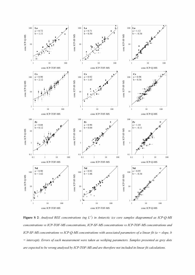
conc ICP-TOF-MS
1 10 100
conc
ICP-
Q-M
S
1
10
100
conc ICP-TOF-MS
1 10 100
conc
ICP-
SF-M
S
1
10
100
conc ICP-Q-MS
1 10 100
conc
ICP-
SF-M
S
1
10
100Laa = 0.72b = 1.11
Laa = 0.71b = 0.50
Laa = 1.12b = - 0.34
conc ICP-TOF-MS
1 10 100
conc
ICP-
Q-M
S
1
10
100
conc ICP-TOF-MS
1 10 100
conc
ICP-
SF-M
S
1
10
100
conc ICP-Q-MS
1 10 100
conc
ICP-
SF-M
S
1
10
100Cea = 0.90b = 2.12
Cea = 0.92b = 1.63
Cea = 0.98b = 0.36
conc ICP-TOF-MS
0.1 1 10 100
conc
ICP-
Q-M
S
0.1
1
10
100
conc ICP-TOF-MS
0.1 1 10 100
conc
ICP-
SF-M
S
0.1
1
10
100
conc ICP-Q-MS
0.1 1 10 100
conc
ICP-
SF-M
S
0.1
1
10
100Pra = 0.88b = 0.12
Pra = 0.90b = 0.04
Pra = 1.10b = - 0.11
conc ICP-TOF-MS
1 10 100
conc
ICP-
Q-M
S
1
10
100
conc ICP-TOF-MS
1 10 100
conc
ICP-
SF-M
S
1
10
100
conc ICP-Q-MS
1 10 100
conc
ICP-
SF-M
S
1
10
100
Nda = 0.90b = 1.62
Nda = 0.92b = 1.06
Nda = 0.95b = - 0.34
Figure S 2: Analysed REE concentrations (ng L-1) in Antarctic ice core samples diagrammed as ICP-Q-MS
concentrations vs ICP-TOF-MS concentrations, ICP-SF-MS concentrations vs ICP-TOF-MS concentrations and
ICP-SF-MS concentrations vs ICP-Q-MS concentrations with associated parameters of a linear fit (a = slope, b
= intercept). Errors of each measurement were taken as weihjing parameters. Samples presented as grey dots
are expected to be wrong analysed by ICP-TOF-MS and are therefore not included in linear fit calculations.
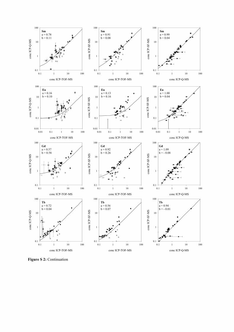
conc ICP-TOF-MS
0.1 1 10 100
conc
ICP-
Q-M
S
0.1
1
10
100
conc ICP-TOF-MS
0.1 1 10 100
conc
ICP-
SF-M
S
0.1
1
10
100
conc ICP-Q-MS
0.1 1 10 100
conc
ICP-
SF-M
S
0.1
1
10
100Sma = 0.78b = 0.11
Sma = 0.91b = 0.08
Sma = 0.99b = 0.04
conc ICP-TOF-MS
0.01 0.1 1 10 100
conc
ICP-
Q-M
S
0.01
0.1
1
10
100
conc ICP-TOF-MS
0.01 0.1 1 10 100
conc
ICP-
SF-M
S
0.01
0.1
1
10
100
conc ICP-Q-MS
0.01 0.1 1 10 100
conc
ICP-
SF-M
S
0.01
0.1
1
10
100Eua = 0.16b = 0.10
Eua = 0.13b = 0.16
Eua = 1.00b = 0.04
conc ICP-TOF-MS
0.1 1 10 100
conc
ICP-
Q-M
S
0.1
1
10
100
conc ICP-TOF-MS
0.1 1 10 100
conc
ICP-
SF-M
S
0.1
1
10
100
conc ICP-Q-MS
0.1 1 10 100
conc
ICP-
SF-M
S
0.1
1
10
100Gda = 0.57b = 0.58
Gda = 0.92b = 0.26
Gda = 1.09b = - 0.08
conc ICP-TOF-MS
0.1 1 10 100
conc
ICP-
Q-M
S
0.1
1
10
100
conc ICP-TOF-MS
0.1 1 10 100
conc
ICP-
SF-M
S
0.1
1
10
100
conc ICP-Q-MS
0.1 1 10 100
conc
ICP-
SF-M
S
0.1
1
10
100Tba = 0.72b = 0.04
Tba = 0.56b = 0.07
Tba = 0.94b = - 0.01
Figure S 2: Continuation

conc ICP-TOF-MS
0.1 1 10 100
conc
ICP-
Q-M
S
0.1
1
10
100
conc ICP-TOF-MS
0.1 1 10 100
conc
ICP-
SF-M
S
0.1
1
10
100
conc ICP-Q-MS
0.1 1 10 100
conc
ICP-
SF-M
S
0.1
1
10
100Dya = 1.00b = 0.25
Dya = 1.02b = 0.13
Dya = 0.93b = - 0.02
conc ICP-TOF-MS
0.01 0.1 1 10
conc
ICP-
Q-M
S
0.01
0.1
1
10
conc ICP-TOF-MS
0.01 0.1 1 10
conc
ICP-
SF-M
S
0.01
0.1
1
10
conc ICP-Q-MS
0.01 0.1 1 10
conc
ICP-
SF-M
S
0.01
0.1
1
10Hoa = 0.82b = 0.08
Hoa = 0.86b = 0.07
Hoa = 1.01b = - 0.04
conc ICP-TOF-MS
0.01 0.1 1 10
conc
ICP-
Q-M
S
0.01
0.1
1
10
conc ICP-TOF-MS
0.01 0.1 1 10
conc
ICP-
SF-M
S
0.01
0.1
1
10
conc ICP-Q-MS
0.01 0.1 1 10
conc
ICP-
SF-M
S
0.01
0.1
1
10Era = 0.99b = 0.10
Era = 1.14b = - 0.04
Era = 1.03b = - 0.07
conc ICP-TOF-MS
0.01 0.1 1 10
conc
ICP-
Q-M
S
0.01
0.1
1
10
conc ICP-TOF-MS
0.01 0.1 1 10
conc
ICP-
SF-M
S
0.01
0.1
1
10
conc ICP-Q-MS
0.01 0.1 1 10
conc
ICP-
SF-M
S
0.01
0.1
1
10Tma = 0.36b = 0.05
Tma = 0.49b = -0.04
Tma = 0.88b = - 0.01
Figure S 2: Continuation

conc ICP-TOF-MS
0.01 0.1 1 10
conc
ICP-
Q-M
S
0.01
0.1
1
10
conc ICP-TOF-MS
0.01 0.1 1 10
conc
ICP-
SF-M
S
0.01
0.1
1
10
conc ICP-Q-MS
0.01 0.1 1 10
conc
ICP-
SF-M
S
0.01
0.1
1
10Yba = 0.93b = 0.05
Yba = 0.99b = - 0.06
Yba = 0.98b = -0.08
Lua = 0.57b = 0.05
conc ICP-TOF-MS
0.001 0.01 0.1 1 10 100
conc
ICP-
Q-M
S
0.001
0.01
0.1
1
10
100Lua = 0.52b = 0.06
conc ICP-TOF-MS
0.001 0.01 0.1 1 10 100
conc
ICP-
SF-M
S
0.001
0.01
0.1
1
10
100Lua = 0.79b = 0.01
conc ICP-Q-MS
0.001 0.01 0.1 1 10 100
conc
ICP-
SF-M
S
0.001
0.01
0.1
1
10
100
Table S 2: Continuation


Paper IV
Proxies and measurement techniques for mineral dustin Antarctic ice cores
Ruth, U., Barbante, C., Bigler, M., Delmonte, B., Fischer, H., Gabrielli,P., Gaspari, V., Kaufmann, P., Lambert, F., Maggi, V., Marino, F.,Petit, J.-R., Steffensen, J.-P., Udisti, R., Wagenbach, D., Wegner, A.,Wolff, E., resubmitted to Environmental Science & Technology.

Proxies and measurement techniques for mineral dust in Antarctic ice cores
Urs Ruth1*, Carlo Barbante2, Matthias Bigler3,4, Barbara Delmonte5, Hubertus
Fischer1, Paolo Gabrielli2,6, Vania Gaspari2, Patrik Kaufmann3, Fabrice Lambert3,
Valter Maggi5, Federica Marino5,7, Jean-Robert Petit8, Roberto Udisti7, Dietmar
Wagenbach9, Anna Wegner1, Eric W. Wolff10
[1] Alfred-Wegener-Institute for Polar and Marine Research, Bremerhaven, Germany
[2] Department of Environmental Sciences, University of Venice, Venice, Italy
[3] Climate and Environmental Physics, Physics Institute, University of Bern, Bern,
Switzerland
[4] Centre for Ice and Climate, Niels Bohr Institute, University of Copenhagen, Denmark
[5] Department of Environmental Sciences, University of Milano Biccoca, Italy
[6] School of Earth Sciences and Byrd Polar Research Center, Ohio State University,
Columbus, USA
[7] Department of Chemistry, University of Florence, Florence, Italy
[8] Laboratoire de Glaciologie et Géophysique de l'Environnement, CNRS, Grenoble, France
[9] Institut für Umweltphysik, University of Heidelberg, Heidelberg, Germany
[10] British Antarctic Survey, Cambridge, United Kingdom

Abstract
To improve quantitative interpretation of ice core aeolian dust records, a systematic
methodological comparison was made. This involved methods for water-insoluble particle
counting (Coulter Counter and laser-sensing particle detector), soluble ion analysis (ion
chromatography, and continuous flow analysis), elemental analysis (inductively coupled
plasma mass spectroscopy at pH 1 and after full acid digestion), and water-insoluble
elemental analysis (proton induced X-ray emission). Antarctic ice core samples covering the
last deglaciation from the EPICA Dome C (EDC) and the EPICA Dronning Maud Land
(EDML) cores were used. All methods correlate very well amongst each other, but the ratios
of glacial age to Holocene concentrations, which are typically a factor ~100, differ between
the methods by up to a factor of 2 with insoluble particles showing the largest variability. The
recovery of ICP-MS measurements depends on the digestion method and is different for
different elements and during different climatic periods. EDC and EDML samples have
similar dust composition, which suggests a common dust source or a common mixture of
sources for the two sites. The analysed samples further reveal a change of dust composition
during the last deglaciation.

1. Introduction
Mineral dust aerosol is an important part of the climate system (1-3). Apart from sea salt it is
the most abundant primary aerosol and influences the radiative energy budget of the
atmosphere (4). Aeolian mineral dust can enhance primary marine bioproductivity (5) and can
be important for pedogenesis in remote land areas (6). To understand the climate changes of
the past it is therefore necessary to have an accurate quantitative reconstruction of the past
atmospheric dust load and aeolian dust fluxes. Projects dedicated to this, such as DIRTMAP
(7), rely on modelling studies and on dust accumulation data from environmental archives.
Although most ice cores come from polar regions – which invokes complex transport
processes from the mid-latitude sources to high-latitude sites – they have a central role as dust
archives because the dust is stored in the simple matrix of ultrapure water and because they
offer excellent time control and temporal resolution.
The most common proxies for dust in ice cores are insoluble particle concentration, e.g. (8-
13), and Ca2+ ion concentration, e.g. (14-18). These have been complemented over recent
years by a large suite of other proxies with multiple measurement techniques for the soluble
and insoluble fraction of the mineral dust aerosol. However, the term “dust” is often used
without exactly specifying the proxy considered, and it is largely unknown how the different
proxies relate quantitatively to each other, particularly under changing climatic conditions.
The objective of this paper is to present a systematic comparison of different proxies and
measurement techniques for mineral dust in ice cores. All techniques investigated use melted
samples; thus techniques based on light scattering on solid ice (19, 20) are omitted. The use of
certified dust samples proved inappropriate because their size distribution, shape, optical
properties, mineralogy and elemental composition differ significantly from aeolian dust
accumulated in polar ice cores. Instead, real ice core samples were used from the two deep
drilling sites of the European Project for Ice Coring in Antarctica (EPICA): EPICA Dome C
(EDC) (21) and EPICA Dronning Maud Land (EDML) (22). Each set of some 20 samples
spans the last glacial termination (Fig. 1), which took place approximately 10-20 ka BP
(thousand years before the present). Thus, the samples cover the full range from low dust
concentrations in the Holocene to high dust concentrations during the Last Glacial Maximum
(LGM) and can also capture possible changes of dust composition over this important
climatic transition. Methodological results from this study are expected to apply also to other
ice cores from Antarctica or Greenland.

2. Methods
Ice samples were decontaminated by three repeated washings in ultra-pure water (Millipore).
The initial weight of each sample was about 200 g, and the mass loss during decontamination
was ~50%. The decontaminated samples were melted at room temperature in pre-washed
LDPE bottles. Once melted, the samples were gently agitated for homogenization and then
partitioned into individual vials (polystyrene Coulter-Counter accuvettes, pre-cleaned using
ultra-pure water) for the different analyses. Repeated checks show that the dust concentration
difference between the first and the last aliquots is typically around the level of measurement-
reproducibility, i.e. the aliquots provided for the different analyses should be comparable.
Exceptionally larger differences (up to 50%) were observed, probably due to contamination of
selected aliquots. The washing and partitioning was performed in a class 100 laminar flow
bench situated inside a class 1000 clean laboratory. The samples dedicated to insoluble
particle analyses were analysed promptly after melting; all other samples were refrozen within
several hours, shipped frozen to the respective laboratories, and kept at -20°C. The samples
were then prepared for the respective analyses (Table 1) as described hereafter.
2.1 Insoluble particles – Coulter Counter (CC)
For Coulter Counter (CC) analysis an electrolyte (NaCl) is added to the sample, which then is
pumped through a small orifice. The electrical conductance is measured across the orifice.
Particles flowing through the orifice reduce the conductance, from which the total volume of
each microparticle is directly estimated. A Multisizer IIe (Beckmann-Coulter) set up in the
clean room of LGGE was used with a 50 μm orifice, allowing measurement of particles with
diameters between 0.7 and 20 μm (256 size channels). Procedures are described elsewhere
(11, 23). Size calibration was achieved via a certified standard of spherical latex particles
(Beckman-Coulter). Each sample was measured three times with 0.5 mL sample volume per
measurement. For calculation of the microparticle mass an average mineral density of 2.5
g/cm3 was assumed.
2.2 Insoluble particles – Laser-sensing Particle Detector (LPD)
A field-portable laser-based detection system LDS 23/25 (Klotz) was used, which was
developed in cooperation with the University of Heidelberg (24). The liquid sample is

pumped through a detection cell, where the attenuation of transmitted light (680 nm) is
measured for each particle (32 channels). Conversion of this signal to particle size is difficult
because complex scattering processes occur. Size assignment was obtained by a posteriori
alignment of the LPD size spectra to the CC size spectra (Ruth et al., in preparation). Using
this procedure, a lower particle detection limit of 1.04 μm diameter was found. The particle
mass below this limit was estimated from a log-normal fit to the data (25) assuming a single-
mode distribution. Each sample was measured three times with 2 mL per measurement. A
mean density of 2.5 g/cm3 was used to convert particle volume to mass.
2.3 Soluble Calcium – Ion Chromatography (IC)
Ion chromatography (IC) is a commercially available method to quantify soluble major ion
concentrations and is well-established for measurement of Ca2+ in ice cores (17, 18, 26). A
sample loop of 1 mL was used with Dionex CG12A and CS12A guard and separation
columns in an isocratic run using methanesulfonate eluent (20mM); low background
conductivity and noise was accomplished using autosuppression (Dionex CSRS Ultra II).
Standardization was achieved by use of cation solutions of certified concentrations. The error
for Ca2+ concentration is strongly dependent on the blank contribution and variability
(typically 1±1 ppb (1 ppb = 1 �g/kg)). With this blank variability, the reproducibility is better
than 10 % for concentrations larger than 20 ppb (i.e. samples from LGM) but increases to
±100 % for concentrations of 1 ppb (i.e. samples from the Holocene). Each sample was
measured once with 3 mL per sample.
2.4 Soluble Calcium – Continuous Flow Analysis (CFA) fluorimetry
CFA is an established technique for continuous measurement of selected ion concentrations at
high spatial resolution in ice cores (27). The analytical method (28) to quantify soluble Ca2+
ion concentrations was adapted at the University of Bern for CFA use (29). In a continuous
flow reactor Ca2+ was converted at pH 7 to a fluorescent complex. The concentration was
deduced from the fluorescence intensity, which was measured by a custom-made
spectrometer at 495 nm wavelength. Standardization was achieved by use of certified Ca2+-
solutions. The method has a detection limit of 0.1 ppb. Typically, the sample water is
obtained continuously from an ice-core melting device, but for this study discrete samples
were injected into the system. Each sample was measured once with ~5 mL per sample.

2.5 Elemental concentrations – Inductively Coupled Plasma Mass Spectrometry
The samples for Inductively Coupled Plasma Mass Spectrometry (ICP-MS) were subdivided
at the University of Venice to compare two different sample preparation methods. For
determination of the “acid-leachable” fractions the samples were melted and acidified to pH 1
with ultrapure nitric acid (Romil) 24 hours prior to the analysis. For determination of the total
content the samples underwent an acid digestion for complete dissolution: to 1 mL of melted
sample were added about 0.3 mL of HNO3 and 0.3 mL of HF (both ultrapure, Romil) with
subsequent microwave irradiation in a PTFE pressure bomb. Procedural blanks were prepared
to check for contamination and values were subtracted from the measured sample
concentrations. Sector field ICP-MS (Element2, Thermo Finnigan) (30, 31) analyses were
performed for aluminum (27Al), vanadium (51V), iron (56Fe) and other trace elements at
medium resolution (m/�m=4000) allowing for separation of major interferences for Fe such
as 40Ar16O. Standardization was achieved using HNO3-acidified and digested dilutions,
respectively, of a multi-element standard (Merck) (32).
2.6 Insoluble element concentrations – Proton Induced X-ray Emission (PIXE)
PIXE is an X-ray spectrometry technique based on primary ionization of the inner shells of a
target atom by an impinging proton beam. The production of characteristic X-rays allows for
highly sensitive bulk dust analysis of elements with atomic numbers ranging from 11 (Na) to
92 (U) (33). For analysis of Antarctic ice dust at very low concentrations, PIXE is able to
measure Na, Mg, Al, Si, K, Ca, Ti, Mn and Fe with analytical detection limits <1 ppb. PIXE
targets were prepared directly by filtering each melted sample through a polycarbonate
membrane (Nuclepore, pore size 0.45 μm) without pre-treatment such as acidification or
precipitation (34). Sample preparation was performed inside a class 100 laminar-flow bench
inside a clean laboratory at the University of Milano-Bicocca. Procedural blanks were
prepared by filtration of ultrapure water following identical procedures. The PIXE analyses
were carried out at the 2 MeV AN2000 accelerator at the National Laboratories of Legnaro
(Padova) (34-36). One target was prepared from each sample with sample volumes from 7 to
50 mL.

3. Results: Methodological Comparison
In total, more than 50 different species related to mineral dust were measured, but only the
most relevant ones are discussed here. In this section, an overview of the results is given first
followed by selected comparisons. Most plots shown are logarithmic scatter plots. Linear
regression lines calculated from the logarithms of the data are also shown: EDML and EDC
data combined (black, continuous line), EDC data only (red, dashed line) and EDML data
only (blue, dotted line). Additionally, in the scatter plots some statistical measures are given;
they are evaluated for the combined sets of EDML and EDC data: Rlog is the correlation
coefficient R calculated from the logarithms of the data. clog is the slope of the linear
regression line calculated from the logarithms of the data; a slope ≠ 1 means that the y/x-ratio
changes with concentration; the values given correspond to the slopes of the black regression
lines. median-ratio is the median of all ratios yi /xi, where yi is the species of the y-axis and xi
is the species of the x-axis for every data point i; median-ratio gives the typical ratio of the y-
parameter to the x-parameter. rel-gain is the relative concentration increase of the y-parameter
for an increase of the x-parameter by a factor f=100; this is a measure of the sensitivity of the
y-parameter to changes of the x-parameter in linear space. rel-gain = 0.5 means that for a 100-
fold increase of the x-parameter the y-parameter increases by 50. Note that rel-gain = f(c_log-1),
i.e. rel-gain does not transform linearly for factors f’≠100.
3.1 Overview of most important proxies and methods
Figure 2 shows a comprehensive overview of scatter plots for different species. For purposes
of comparability, they are all plotted against a common reference, for which insoluble particle
concentrations (from CC) are chosen. The dust concentration in the EDML-samples is
typically 2-3 times that of EDC-samples. Insoluble particles exhibit the largest concentration
variance of all species shown; the ratio between highest glacial and lowest Holocene particle
concentration is about 200 (119 for EDC and 337 for EDML for the particular sets of samples
from this study). All chemical species exhibit a good correlation with insoluble particles,
typically Rlog > 0.9. However, clog is > 0.8, and rel-gain > 0.5 for most species, which means
that the y/x-ratio is up to a factor of 2 lower at high than at low concentrations. This indicates
considerable changes in dust composition or detection between the climate regimes. Thus, a
quantitative reconstruction of dust deposition fluxes will depend on the particular choice of
the parameter.
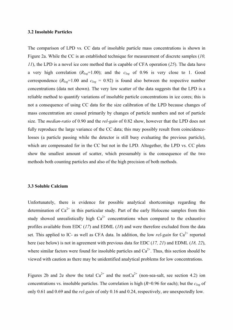
3.2 Insoluble Particles
The comparison of LPD vs. CC data of insoluble particle mass concentrations is shown in
Figure 2a. While the CC is an established technique for measurement of discrete samples (10,
11), the LPD is a novel ice core method that is capable of CFA operation (25). The data have
a very high correlation (Rlog=1.00); and the clog of 0.96 is very close to 1. Good
correspondence (Rlog=1.00 and clog = 0.92) is found also between the respective number
concentrations (data not shown). The very low scatter of the data suggests that the LPD is a
reliable method to quantify variations of insoluble particle concentrations in ice cores; this is
not a consequence of using CC data for the size calibration of the LPD because changes of
mass concentration are caused primarily by changes of particle numbers and not of particle
size. The median-ratio of 0.90 and the rel-gain of 0.82 show, however that the LPD does not
fully reproduce the large variance of the CC data; this may possibly result from coincidence-
losses (a particle passing while the detector is still busy evaluating the previous particle),
which are compensated for in the CC but not in the LPD. Altogether, the LPD vs. CC plots
show the smallest amount of scatter, which presumably is the consequence of the two
methods both counting particles and also of the high precision of both methods.
3.3 Soluble Calcium
Unfortunately, there is evidence for possible analytical shortcomings regarding the
determination of Ca2+ in this particular study. Part of the early Holocene samples from this
study showed unrealistically high Ca2+ concentrations when compared to the exhaustive
profiles available from EDC (17) and EDML (18) and were therefore excluded from the data
set. This applied to IC- as well as CFA data. In addition, the low rel-gain for Ca2+ reported
here (see below) is not in agreement with previous data for EDC (17, 21) and EDML (18, 22),
where similar factors were found for insoluble particles and Ca2+. Thus, this section should be
viewed with caution as there may be unidentified analytical problems for low concentrations.
Figures 2b and 2e show the total Ca2+ and the nssCa2+ (non-sea-salt, see section 4.2) ion
concentrations vs. insoluble particles. The correlation is high (R=0.96 for each); but the clog of
only 0.61 and 0.69 and the rel-gain of only 0.16 and 0.24, respectively, are unexpectedly low.
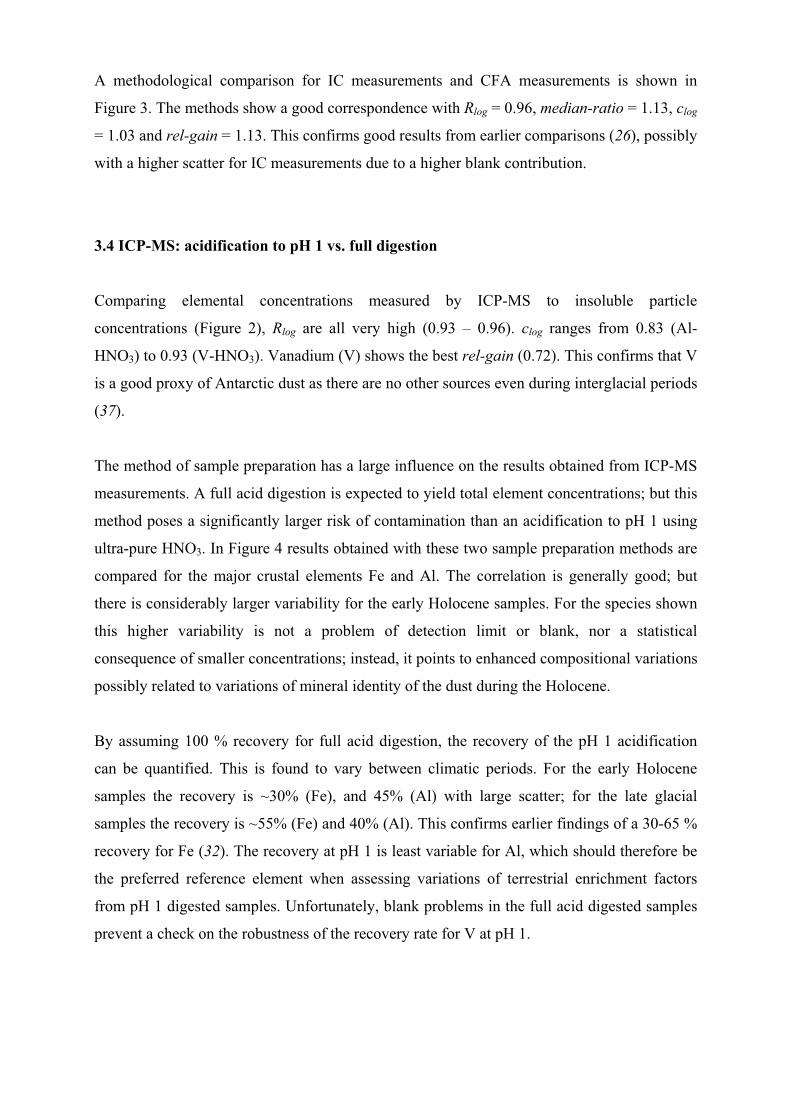
A methodological comparison for IC measurements and CFA measurements is shown in
Figure 3. The methods show a good correspondence with Rlog = 0.96, median-ratio = 1.13, clog
= 1.03 and rel-gain = 1.13. This confirms good results from earlier comparisons (26), possibly
with a higher scatter for IC measurements due to a higher blank contribution.
3.4 ICP-MS: acidification to pH 1 vs. full digestion
Comparing elemental concentrations measured by ICP-MS to insoluble particle
concentrations (Figure 2), Rlog are all very high (0.93 – 0.96). clog ranges from 0.83 (Al-
HNO3) to 0.93 (V-HNO3). Vanadium (V) shows the best rel-gain (0.72). This confirms that V
is a good proxy of Antarctic dust as there are no other sources even during interglacial periods
(37).
The method of sample preparation has a large influence on the results obtained from ICP-MS
measurements. A full acid digestion is expected to yield total element concentrations; but this
method poses a significantly larger risk of contamination than an acidification to pH 1 using
ultra-pure HNO3. In Figure 4 results obtained with these two sample preparation methods are
compared for the major crustal elements Fe and Al. The correlation is generally good; but
there is considerably larger variability for the early Holocene samples. For the species shown
this higher variability is not a problem of detection limit or blank, nor a statistical
consequence of smaller concentrations; instead, it points to enhanced compositional variations
possibly related to variations of mineral identity of the dust during the Holocene.
By assuming 100 % recovery for full acid digestion, the recovery of the pH 1 acidification
can be quantified. This is found to vary between climatic periods. For the early Holocene
samples the recovery is ~30% (Fe), and 45% (Al) with large scatter; for the late glacial
samples the recovery is ~55% (Fe) and 40% (Al). This confirms earlier findings of a 30-65 %
recovery for Fe (32). The recovery at pH 1 is least variable for Al, which should therefore be
the preferred reference element when assessing variations of terrestrial enrichment factors
from pH 1 digested samples. Unfortunately, blank problems in the full acid digested samples
prevent a check on the robustness of the recovery rate for V at pH 1.

3.5 PIXE
Comparing elemental concentrations measured by PIXE to insoluble particle concentrations
(Figure 2) Rlog ranges from 0.92 (Al) to 0.97 (Si, Fe) with clog from 0.8 (Ca) to 0.97 (Si). For
Ca (Figure 2c) low concentration data give a different ratio between the two methods for EDC
and EDML; however, concentrations are close to the detection limit.
PIXE measures the elemental composition of water-insoluble dust after filtration. By
assuming 100 % filtration efficiency for PIXE and 100 % recovery for ICP-MS measurements
(full acid digestion), the elements Fe and Al can be attributed to a water-insoluble fraction and
a soluble residual. In Figure 5 results obtained with the two methods are compared.
For Fe a very good log-correlation is found (Rlog =0.95) with clog =1.0. The median-ratio is
0.76, suggesting that ~25% of the Fe is water-soluble. This ratio does not change between
glacial times and early Holocene. The upper limit for the fraction of bio-available iron, which
still depends on the oxidation state, would thus be ~25%, which is larger by a factor 5-10 than
the values typically used in models for simulating the effect of iron-fertilization in the
Southern Ocean (38-40).
For Al the insoluble fraction amounts to ~100 %. However, early Holocene samples show a
large scatter (especially for EDC-samples) with PIXE concentrations exceeding the ICP-MS
concentrations. This may be caused by analytical uncertainties with the ICP-MS full acid
digestion method in this case.
A comparison between CFA-Ca (Figure 2b, mean concentration ~10 ppb) and PIXE-Ca
(Figure 2c, mean concentration ~1 ppb) suggests that ~ 90 % Ca is present in soluble form
while only 10 % are water-insoluble; this confirms and quantifies earlier findings (3, 15, 35).
4. Discussion of dust composition
The most noticeable observation from Figures 2-5 is that no obvious systematic differences
occur between EDC and EDML samples. In all scatter plots shown the samples from EDC
and EDML overlap strongly and do not fall into separate groups. An exception is PIXE-Ca
data during early Holocene, however, values are close to the detection limit and thus

questionable. This suggests that the dust composition is geochemically very similar at the two
sites and that they likely receive dust from a common dust source or the same mixture of
sources as has been suggested also for other locations (41).
The mean composition of the insoluble dust can be characterized by referring elemental
concentrations determined by PIXE to the total particle mass from CC. This yields mean
ratios of approximately 0.26 (Si), 0.08 (Al), and 0.05 (Fe), which deviate only slightly from
the mean composition of upper continental crust of 0.30 (Si), 0.08 (Al), and 0.03 (Fe) (42).
Detailed compositional investigations should be made using material from potential dust
sources and focussing on fractionation during uptake, atmospheric transport and dissolution.
Although the mean composition for Si, Al, Fe and Ca as referenced to CC insoluble particle
mass give reasonable results similar to crustal averages, the rel-gain is always below 1. This
could imply that either the dust is depleted in these elements at high or enriched at low
concentrations, possibly resulting from fractionation during transport. Alternatively, there
could be analytical issues, and further work is needed to clarify this issue.
4.1 Terrestrial vs. marine contributions to Ca2+ and Na+
Ca2+ and Na+ contain soluble terrestrial contributions from mineral dust and marine
contributions from sea salt. To evaluate these contributions separately the respective mass
ratios (Na/Ca)sol,dust of soluble Na+ and Ca2+ from mineral dust and (Na/Ca)ss from sea salt
aerosol must be known. (Na/Ca)ss ranges between 23 (brine rejected during sea ice formation
(43)) and 26 (bulk sea water (44)). However, (Na/Ca)sol,dust is far more variable and less well
known.
The apportionment of Ca2+ into a “non sea salt” fraction (nssCa) and a “sea salt” fraction
(ssCa) often considers (Na/Ca)sol,dust = 0.56 (e.g. (3, 45)), which corresponds to the total (not
only soluble) elemental composition of mean continental crust (44). Alternatively, total
element ratios for upper continental crust could be used (Na/Ca=0.87) (42) ; and from high-
resolution ice core data (Na/Ca)sol,dust = 0.94±0.07 is suggested (46). Here we take another
complementary approach based on linking insoluble dust, Ca2+ and Na+ concentrations. The
following equations are considered: [Ca2+] = [Cass] + [Casol,dust] = �-1 [Nass] + a [CC], where �
= (Na/Ca)ss is chosen to be 26 (� = 23 gives the same results for b), a = [Casol,dust] / [CC], and
[CC] is the insoluble particle mass concentration. Further, [Na+] = [Nass] + [Nasol,dust] = [Nass]
+ ab [CC], where b = (Na/Ca)sol,dust is the parameter of interest. Parameter optimization yields
b = 0.91±0.2 (a = 0.085) for all samples from this study [b = 1.05 (a = 0.057) for samples
dated older than 16 ka BP to circumvent potential problems with Holocene Ca2+ data, and b =
0.83 (a = 0.092) for samples dated younger than 16 ka BP]. Thus, we suggest an average of
(Na/Ca)sol,dust = 0.91±0.2 by mass, which is in good agreement with (46).
4.2 Temporal changes of dust composition
Compositional changes of the ice core dust over time can be identified by calculating ratios
between different dust-related parameters on identical ice-core samples. Figure 6 shows time
series of selected ratios on the common EDML1/EDC3 time scale (47, 48): the recovery of
ICP-MS measurements for sample preparation at pH 1 for Fe and Al, the Fe/Al ratio at pH 1,
and the element ratios Si/Al and K/Al from PIXE. It is clearly noticeable that a regime-shift
happens during the deglaciation. The sample-to-sample variability of the ratios is much higher
for the early Holocene samples than for the late glacial samples. Also, the average recovery of
acidified samples (pH 1) measured by ICP-MS changes during the deglaciation, albeit less
prominently. Further, the insoluble elemental composition of the dust (PIXE) shifts to
relatively more Al, less Si and less K.
A change in dust mineralogy during the last deglaciation is consistent with other observations:
A similar shift to less K and more Ca in the Taylor Dome ice core (49), and a difference of
Nd and Sr isotope ratios at EDC (50) and a change of Li solubility at EDC (51). This regime
shift dates between ~16.5 and ~15.0 ka BP from our data. It suggests that either the
characteristics of the dust source changes (e.g. soil development), or there is a change in the
relative contributions of different sources (e.g. transport changes). The overlap of EDC and
EDML samples indicates that even at times of higher variability there are no distinct sources
and transport paths to the two ice core sites. Thus, the controlling factors for dust
concentrations on the East Antarctic plateau likely are the emission intensity in the dust
sources as well as the ability of the dust to intrude the polar vortex. Once inside the polar
vortex the dust transport to the two sites is either very homogeneous or effectively
randomized.

Acknowledgements
This work is a contribution to the European Project for Ice Coring in Antarctica (EPICA), a
joint European Science Foundation/European Commission scientific programme, funded by
the EU and by national contributions from Belgium, Denmark, France, Germany, Italy, the
Netherlands, Norway, Sweden, Switzerland and the United Kingdom. The main logistic
support was provided by IPEV and PNRA (at Dome C) and AWI (at Dronning Maud Land).
This is EPICA publication no. 196. Data are available from Pangaea
(doi:10.1594/PANGAEA.xxxxxx).

References
1. Prospero, J. M.; Charlson, R. J.; Mohnen, V.; Jaenicke, R.; Delany, A. C.; Moyers, J.; Zoller, W.; Rahn, K., The atmospheric aerosol systen: an overview. Reviews of Geophysics and Space Physics 1983, 21, (7), 1607-1629.
2. Rea, D. K., The paleoclimatic record provided by eolian deposition in the deep sea: the geologic history of wind. Reviews of Geophysics 1994, 32, (2), 159-195.
3. Fischer, H.; Siggaard-Andersen, M. L.; Ruth, U.; Röthlisberger, R.; Wolff, E., Glacial/interglacial changes in mineral dust and sea-salt records in polar ice cores: Sources, transport, and deposition. Reviews of Geophysics 2007, 45, (RG1002), doi:10.1029/2005RG000192.
4. Sokolik, I. N.; Winker, D. M.; Bergametti, G.; Gillette, D. A.; Carmichael, G.; Kaufman, Y. J.; Gomes, L.; Schuetz, L.; Penner, J. E., Introduction to special section: Outstanding problems in quantifying the radiative impacts of mineral dust. Jourmal of Geophysical Research 2001, 106, (D16), 18015-18027.
5. Boyd, P. W.; Jickells, T.; Law, C. S.; Blain, S.; Boyle, E. A.; Buesseler, K. O.; Coale, K. H.; Cullen, J. J.; de Baar, H. J. W.; Follows, M.; Harvey, M.; Lancelot, C.; Levasseur, M.; Owens, N. P. J.; Pollard, R.; Rivkin, R. B.; Sarmiento, J.; Schoemann, V.; Smetacek, V.; Takeda, S.; Tsuda, A.; Turner, S.; Watson, A. J., Mesoscale Iron Enrichment Experiments 1993-2005: Synthesis and Future Directions. Science 2007, 315, 612-617, DOI: 10.1126/science.1131669.
6. Wang, P.; Clemens, S. C.; Beaufort, L.; Branconnot, P.; Ganssen, G. M.; Jian, Z.; Kershaw, P.; Sarnthein, M., Evolution and variability of the Asian monsoon system: State of the art and outstanding issues. Quaternary Science Reviews 2005, 24, 595-629.
7. Kohfeld, K. E.; Harrison, S. P., DIRTMAP: the geological record of dust. Earh-Science Reviews 2001, 54, 81-114.
8. Cragin, J. H.; Herron, M. M.; Langway Jr., C. C.; Klouda, G., Interhemispheric comparison of changes in the composition of atmospheric precipitation during the late Cenozoic era. In Polar Oceans, Dunbar, M. J., Ed. Arctic Institute of North America: Calgary, AB, Canada, 1977; pp 617-631.
9. Hammer, C. U. In Dust studies on Greenland ice cores, Isotopes and impurities in snow and ice-symposium, Proceedings of the Grenoble Symposium, 1977; Proceedings of the Grenoble Symposium, 1977; pp 365-370.
10. Petit, J.-R.; Briat , M.; Royer, A., Ice age aerosol content from East Antarctic ice core samples and past wind strenght. Nature 1981, 293, 391-394.
11. Steffensen, J. P., The size distribution of microparticles from selected segments of the Greenland Ice Core Project ice core representing different climatic periods. Journal of Geophysical Research 1997, 102, (C12), 26755-26763.
12. Delmonte, B.; Basile-Doelsch, I.; Petit, J.-R.; Maggi, V.; Revel-Rolland, M.; Michard, A.; Jagoutz, E.; Grousset, F. E., Comparing the EPICA and Vostok dust records during the last 220,00 years: stratigraphical correlation and provenance in glacial periods. Earh-ScienceReviews 2004, 66, 63-87.

13. Lambert, F.; Delmonte, B.; Petit, J.-R.; Bigler, M.; Kaufmann, P.; Hutterli, M. A.; Stocker, T.; Ruth, U.; Steffensen, J. P.; Maggi, V., Dust-climate couplings over the past 800,000 years from the EPICA Dome C ice core. Nature 2007, in review.
14. Legrand, M.; Delmas, R., Soluble impurities in four Antarctic ice cores over the last 30000 years. Annals of Glaciology 1988, 10, 116-120.
15. de Angelis, M.; Barkov, N. I.; Petrov, V. N., Sources of continental dust over Antarctica during the last glacial cycle. Journal of Atmospheric Chemistry 1992, 14, 233-244.
16. Mayewski, P. A.; Meeker, L. D.; Whitlow, S.; Twickler, M. S.; Morrison, M. C.; Bloomfield, P.; Bond, G. C.; Alley, R. B.; Gow, A. J.; Grootes, P. M.; Meese, D. A.; Ram, M.; Taylor, K. C.; Wumkes, W., Changes in atmospheric circulation and ocean ice cover over the North Atlantic during the last 41,000 years. Science 1994, 263, 1747-1751.
17. Wolff, E. W.; Fischer, H.; Fundel, F.; Ruth, U.; Twarloh, B.; Littot, G.; Mulvaney, R.; Röthlisberger, R.; de Angelis, M.; Boutron, C.; Hansson, M.; Jonsell, U.; Hutterli, M.; Bigler, M.; Lambert, F.; Kaufmann, P.; Stauffer, B.; Steffensen, J. P.; Siggaard-Andersen, M. L.; Udisti, R.; Becagli, S.; Castellano, E.; Severi, M.; Wagenbach, D.; Barbante, C.; Gabrielli, P.; Gaspari, V., Southern Ocean sea-ice extent, productivity and iron flux over the past eight glacial cycles. Nature 2006, 440, 491-496, doi:10:1038/nature04614.
18. Fischer, H.; Fundel, F.; Ruth, U.; Twarloh, B.; Wegner, A.; Udisti, R.; Becagli, S.; Castellano, E.; Morganti, A.; Severi, M.; Wolff, E.; Littot, G.; Röthlisberger, R.; Mulvaney, R.; Hutterli, A.; Kaufmann, P.; Federer, U.; Lambert, F.; Bigler, M.; Hansson, M.; Jonsell, U.; de Angelis, M.; Gabrielli, P.; Boutron, C.; Siggaard-Andersen, M. L.; Steffensen, J. P.; Barbante, C.; Gaspari, V.; Gabrielli, P.; Wagenbach, D., Reconstruction of millenial changes in dust emission, transport and regional sea ice coverage using the deep EPICA ice cores from the Atlantic and Indian Ocean sectors of Antarctica. Earth and Planetary Science Letters 2007, 260, 340-354.
19. Bay, R. C.; Price, B. P.; Clow, G. D.; Gow, A. J., Climate logging with a new rapid optical technique at Siple Dome. Geophysical Research Letters 2001, 28, (24), 4635-4638.
20. Ram, M.; Koenig, G., Continuous dust concentration profile of pre-Holocene ice from the Greenland Ice Sheet Projct 2 ice core: dust stadials, interstadials, and the Eemian. Journalof Geophysical Research 1997, 102, (C12), 26641-26648.
21. EPICA-community-members, Eight glacial cycles from an Antarctic ice core. Nature2004, 429, 623-628, doi:10.1038/nature02599.
22. EPICA-community-members, One-to-one coupling of glacial climate variability in Greenland and Antarctica. Nature 2006, 444, 195-198, doi:10.1038/nature05301.
23. Delmonte, B.; Petit, J. R.; Maggi, V., Glacial to Holocene implications of the new 27,000-year dust record from the EPICA Dome C (East Antarctica) ice core. ClimateDynamics 2002, 18, (8), 647-660.
24. Ruth, U.; Wagenbach, D.; Bigler, M.; Steffensen, J. P.; Röthlisberger, R.; Miller, H., High resolution dust profiles at NGRIP: Case studies of the calcium-dust relationship. Annalsof Glaciology 2002, 35, 209–216.
25. Ruth, U.; Wagenbach, D.; Steffensen, J. P.; Bigler, M., Continuous record of microparticle concentration and size distribution in the central Greenland NGRIP ice core during the lastglacial period. Journal of Geophysical Research 2003, 108, (D3), doi:10.1029/2002JD002376.

26. Littot, G.; Mulvaney, R.; Röthlisberger, R.; Udisti, R.; Wolff, E.; Castellano, E.; de Angelis, M.; Hansson, M. E.; Sommer, S.; Steffensen, J. P., Comparison of analytical methods used for measuring mahor ions in the EPICA Dome C (Antarctica) ice core. Annals of Glaciology 2002, 35, 299-305.
27. Röthlisberger, R.; Bigler, M.; Hutterli, A.; Sommer, S.; Stauffer, B.; Junghans, H. G.; Wagenbach, D., Technique for continuous high-resolution analysis of trace substances in firn and ice cores. Environmental Science and Technology 2000, 34, 338-342.
28. Tsien, R. Y.; Pozzan, T.; Rink, T. J., Calcium homeostasis in intact lymphocytes: cyroplasmic free calcium monitored with a new, intracellularly trapped fluorecent indicator. The Journal of Cell Biology 1982, 94, 325-334.
29. Sigg, A.; Fuhrer, K.; Anklin, M.; Staffelbach, T.; Zurmühle, D., A continuous analysis technique for trace species in ice cores. Environmental Science and Technology 1994, 28, 204-210.
30. Barbante, C.; Cozzi, G.; Capodaglio, G.; van de Velde, K.; Ferrari, C.; Boutron, C.; Cescon, P., Trace element determination in alpine snow and ice by double focussing inductively coupled plasma spectrometry. J. Anal. At. Spectrom. 1999, 14, 1433.
31. Planchon, F. A. M.; Boutron, C.; Barbante, C.; Wolff, E. W.; Cozzi, G.; Gaspari, V.; Ferrari, C.; Cescon, P., Ultrasensitive determination of heavy metals at the sub-picogram per gram level in ultraclean Antarctic snow samples by inductively coupled plasma sector field mass spectrometry. Analytica Chimica Acta 2001, 450, (1), 193-205.
32. Gaspari, V.; Barbante, C.; Cozzi, G.; Cescon, P.; Boutron, C.; Gabrielli, P.; Capodaglio, G.; Ferrari, C.; Petit, J. R.; Delmonte, B., Atmospheric iron fluxes over the last deglaciation: climatic implications. Geophysical Research Letters 2006, 33, L03704, doi:10.1029/2005GL024352.
33. Johansson, S. A. E.; Campbell, J. L.; Malmqvist, K. L., Particle induced X-ray emission (PIXE). John Wiley and Sons, Inc.: New York, 1995.
34. Marino, F.; Maggi, V.; Delmonte, B.; Ghermandi, G.; Petit, J.-R., Elemental composition (Si, Fe, Ti) of atmospheric dust over the last 220 kyr from the EPICA ice core (Dome-C, Antactica). Annals of Glaciology 2004, 39, 110-118.
35. Ghermandi, G.; Cecchi, R.; Capotosto, M.; Marino, F., Elemental composition determined by PIXE analysis of the insoluble aerosol particles in EPICA-Dome C ice core samples representing the last 27000 years. Geophysical Research Letters 2003, 30, (22), doi:10.1029/2003GL018169.
36. Marino, F. Geochemical chracterization of the EPICA Dome-C ice core dust by major elements PIXE analysis and its paleoclimatic implications. PhD thesis, University of Siena, Siena, 2006.
37. Gabrielli, P.; Planchon, F.; Hong, S.; Lee, K.; Hur, S. D.; Barbante, C.; Ferrari, C.; Petit, J.-R.; Lipenkov, V. Y.; Cescon, P.; Boutron, C., Trace elements in Vostok Antarctic ice during the last four climatic cycles. Earth and Planetary Science Letters 2005, 234, (1-2), 249-259.
38. Moore, J. K.; Doney, S. C.; Lindsay, K., Upper ocean ecosystem dynamics and iron cycling in a global three-dimensional model. Global Biogeochemical Cycles 2004, 18, (GB4028), doi:10.1029/2004GB002220.

39. Fung, I. Y.; Meyn, S. K.; Tegen, I.; Doney, S. C.; John, J. G.; Bishop, K. B., Iron supply and demand in the upper ocean. Global Biogeochemical Cycles 2000, 14, (1), 281-295.
40. Cassar, N.; Bender, M. L.; Barnett, B. A.; Fan, S.; Moxim, W. J.; Il, H. L.; Tilbrook, B., The Southern Ocean Biological Response to Aeolian Iron Deposition. Science 2007, 317, 1067-1070, DOI: 10.1126/science.1144602.
41. Hinkley, T.; Pertsiger, F.; Zavjalova, L., The modern atmospheric background dust load: recognition in Central Asian snowpack, and compositional contraints. Geophysical Research Letters 1997, 24, (13), 1607-1610.
42. Wedepohl, K. H., The composition of the continental crust. Geochim. Cosmochim. Acta 1995, 59, (7), 1217-1232.
43. Wagenbach, D.; Ducroz, F.; Mulvaney, R.; Keck, L.; Minikin, A.; Legrand, M.; Hall, J. S.; Wolff, E. W., Sea-salt aerosol in coastal Antarctic regions. Journal of Geophysical Research 1998, 103, (D9), 10961-10974.
44. Bowen, H. J. M., Environmental Chemistry of the Elements. Academic Press: London, 1979.
45. Röthlisberger, R.; Mulvaney, R.; Wolff, E.; Hutterli, M.; Bigler, M.; Sommer, S.; Jouzel, J., Dust and sea salt variability in central East Antarctica (Dome C) over the last 45 kyrs and its implications for southern high-latitude climate. Geophysical Research Letters 2002, 29, (20), 1963, doi:10.1029/2002GL015186.
46. Bigler, M.; Röthlisberger, R.; Lambert, F.; Stocker, T.; Wagenbach, D., Aerosol deposited in East Antarctica over hte last glacial cycle: Detailed apportionment of continental and sea-salt contributions. Journal of Geophysical Research 2006, 111, (D08205), doi:10.1029/2005JD006469.
47. Ruth, U.; Barnola, J.-M.; Beer, J.; Bigler, M.; Blunier, T.; Castellano, E.; Fischer, H.; Fundel, F.; Huybrechts, P.; Kaufmann, P.; Kipfstuhl, S.; Lambrecht, A.; Morganti, A.; Parrenin, F.; Rybak, O.; Severi, M.; Udisti, R.; Wilhelms, F.; Wolff, E., EDML1: A chronology for the EPICA deep ice core from Dronning Maud Land, Antarctica, over the last 150,000 years. Climate of the Past 2007, 3, 475-484.
48. Parrenin, F.; Barnola, J.-M.; Beer, J.; Blunier, T.; Castellano, E.; Chappellaz, J.; Dreyfus, G.; Fischer, H.; Fujita, S.; Jouzel, J.; Kawamura, K.; Lemieux, B.; Loulergue, L.; Masson-Delmotte, V.; Narcisi, B.; Petit, J.-R.; Raisbeck, G.; Raynaud, D.; Ruth, U.; Schwander, J.; Severi, M.; Spahni, R.; Steffensen, J. P.; Svensson, A.; Udisti, R.; Waelbroeck, C.; Wolff, E., The EDC3 chronology for the EPICA Dome C ice core. Climate of the Past 2007, 3, 485-497.
49. Hinkley, T.; Matsumoto, A., Atmospheric regime of dust and salt through 75,000 years of Taylor Dome ice core: Refinement by measurement of mahor, minor, and trace metal suites. Journal of Geophysical Research 2001, 106, (D16), 18487-18493.
50. Delmonte, B.; Petit, J.-R.; Basile-Doelsch, I.; Jagoutz, E.; Maggi, V., Late Quaternary Interglacials in East Antarctica from ice core dust records. In The Climate of Past Interglacials, Sirocko, F.; Litt, T.; Claussen, M., Eds. Elsevier: Amsterdam, 2006.
51. Siggaard-Andersen, M. L.; Gabrielli, P.; Steffensen, J. P.; Stromfeldt, T.; Barbante, C.; Boutron, C.; Fischer, H.; Miller, H., Soluble and insoluble lithium dust in the EPICA DomeC ice core - Implications for changes of the East Antarctic dust provenance during the recent glacial-interglacial transition. Earth and Planetary Science Letters 2007, 258, 32-43.

Tables and Figures with Captions
Table 1 – Parameter overview: List of species and measurement methods of mineral dust
discussed in this paper; also given are the respective limits of detection (LOD, including
procedural blanks) for typical applications.
Acronym Species Method LOD [ppb]CC-mass total water-insoluble particle mass (from
particle volume) Coulter Counter 2
LPD-mass total water-insoluble particle mass (from particle diameter)
Laser-sensing Particle Detector
1
IC-Ca soluble Ca2+ Ion Chromatography 2 CFA-Ca soluble Ca2+ Continuous Flow
Analysis0.1
nss-CFA-Ca* soluble non-sea-salt Ca2+ [(Na/Ca)sol,dust = 0.91] calculated --- ICPMS-digest-Al total Al (full acid digestion) ICP-MS 0.5 ICPMS-digest-Fe total Fe (full acid digestion) ICP-MS 0.2 ICPMS- HNO3-Al leachable Al (HNO3-digestion at pH 1) ICP-MS 0.1 ICPMS- HNO3-Fe leachable Fe (HNO3-digestion at pH 1) ICP-MS 0.03 ICPMS- HNO3-V leachable V (HNO3-digestion at pH 1) ICP-MS 0.001 PIXE-Al water-insoluble, particulate dust Al PIXE 0.8PIXE-Ca water-insoluble, particulate dust Ca PIXE 0.2PIXE-Fe water-insoluble, particulate dust Fe PIXE 0.1PIXE-Si water-insoluble, particulate dust Si PIXE 0.7
Table 1.

Figure 1:
0 10 20 30 40 50-450
-400
EDML1/EDC3-Age (ka BP)
δD (‰
) bHolocene Glacial period
100
102
104
Dus
t con
c. (p
pb) aEDC
EDML
Figure 1:
Upper panel (a): Overview of samples used in this study shown on the EDML1/EDC3 time
scale (47, 48); EDC samples shown as dark red asterisks, EDML samples shown as blue
circles. Insoluble particle mass concentrations (CC-mass) are plotted here as a representative
of mineral dust concentrations. For orientation, the EDC dust profile is also shown as a red
line (12). Note that samples range from low concentrations during Holocene to high
concentrations during the LGM for EDC as well as for EDML. Lower panel (b): For
orientation, EDC deuterium isotopic deviation as a proxy for atmospheric temperature (21).

100 101 102 103 104100
101
102
103
104
CC-mass (ppb)
LPD
-mas
s (p
pb)
Rlog = 1.00 clog = 0.96 median ratio=0.897rel gain = 0.82
a
EDCEDML
100 101 102 103 10410-4
10-3
10-2
10-1
100
CC-mass (ppb)
ICPM
S-H
NO
3-V
(ppb
)
Rlog = 0.96 clog = 0.93 median ratio=0.000rel gain = 0.72
d
EDCEDML
100 101 102 103 10410-1
100
101
102
103
CC-mass (ppb)
CFA
-Ca
(ppb
)
Rlog = 0.96 clog = 0.61 median ratio=0.060rel gain = 0.16
b
EDCEDML
100 101 102 103 10410-1
100
101
102
103
CC-mass (ppb)
nss-
CFA
-Ca
(ppb
)
Rlog = 0.96 clog = 0.69 median ratio=0.053rel gain = 0.24
e
EDCEDML
100 101 102 103 10410-2
10-1
100
101
102
CC-mass (ppb)
PIXE
-Ca
(ppb
)
Rlog = 0.93 clog = 0.80 median ratio=0.009rel gain = 0.40
c
EDCEDML
100 101 102 103 10410-1
100
101
102
103
CC-mass (ppb)
PIXE
-Si (
ppb)
Rlog = 0.97 clog = 0.97 median ratio=0.261rel gain = 0.87
f
EDCEDML
Figure 2 a-f:

100 101 102 103 10410-2
10-1
100
101
102
CC-mass (ppb)
ICPM
S-H
NO
3-Fe
(ppb
)
Rlog = 0.95 clog = 0.90 median ratio=0.025rel gain = 0.62
g
EDCEDML
100 101 102 103 10410-1
100
101
102
103
CC-mass (ppb)
ICPM
S-H
NO
3-Al
(ppb
)
Rlog = 0.96 clog = 0.83 median ratio=0.044rel gain = 0.46
j
EDCEDML
100 101 102 103 10410-1
100
101
102
103
CC-mass (ppb)
ICPM
S-di
gest
-Fe
(ppb
)
Rlog = 0.96 clog = 0.87 median ratio=0.057rel gain = 0.54
h
EDCEDML
100 101 102 103 10410-1
100
101
102
103
CC-mass (ppb)
ICPM
S-di
gest
-Al (
ppb)
Rlog = 0.93 clog = 0.84 median ratio=0.095rel gain = 0.47
k
EDCEDML
100 101 102 103 10410-1
100
101
102
103
CC-mass (ppb)
PIXE
-Fe
(ppb
)
Rlog = 0.97 clog = 0.93 median ratio=0.045rel gain = 0.73
i
EDCEDML
100 101 102 103 10410-1
100
101
102
103
CC-mass (ppb)
PIXE
-Al (
ppb)
Rlog = 0.92 clog = 0.82 median ratio=0.081rel gain = 0.44
l
EDCEDML
Figure 2 g-l:
Figure 2:
Scatter plots of different parameters all plotted vs. insoluble particle mass (from Coulter
Counter) as a common reference for comparison. All values in ppb. Note logarithmic scales.
Shown also are linear regression lines calculated from the logarithms of the data: EDML and
EDC data (black continuous line), EDC data only (red, dashed line) and EDML data only
(blue, dotted line). Selected statistical measures are given in each plot for all (EDC and
EDML) data: Rlog – correlation coefficient (in loglog-space); clog – slope of linear regression
line (in loglog-space); median ratio – median of ratios (yi/xi) of concentrations; rel gain –
relative gain of y-parameter for a concentration increase of factor 100 for the x-parameter. For
details see text; for abbreviations of parameters: see Table 1.

Figure 3:
100 101 102100
101
102
IC-Ca (ppb)
CFA
-Ca
(ppb
)
Rlog = 0.96 clog = 1.03 median ratio=1.129rel gain = 1.13
EDCEDML
Figure 3:
Scatter plot of CFA-Ca2+ vs. IC-Ca2+.

Figure 4:
Figure 4:
Scatter plot of ICP-MS element concentrations of Fe (a) and Al (b) for two different sample
preparation techniques: acidification to pH 1 (y-axis) vs. full acid digestion (x-axis). Typical
recoveries of HNO3-digestion (pH 1) are indicated for Holocene and LGM samples (see text
for details).
10-1 100 101 102 10310-2
10-1
100
101
102
ICPMS-digest-Fe (ppb)
ICPM
S-H
NO
3-Fe
(ppb
)
Rlog = 0.95 clog = 0.98 median ratio=0.458rel gain = 0.92
a
30%
55%EDCEDML
10-1 100 101 102 10310-1
100
101
102
103
ICPMS-digest-Al (ppb)IC
PMS-
HN
O3-
Al (p
pb)
Rlog = 0.97 clog = 0.94 median ratio=0.415rel gain = 0.76
b
45%
40%
EDCEDML
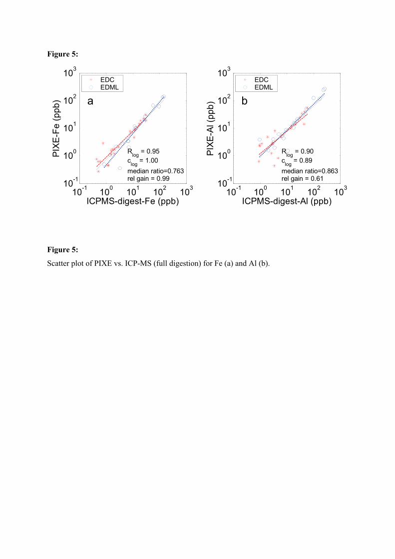
Figure 5:
10-1 100 101 102 10310-1
100
101
102
103
ICPMS-digest-Fe (ppb)
PIXE
-Fe
(ppb
)
Rlog = 0.95 clog = 1.00 median ratio=0.763rel gain = 0.99
a
EDCEDML
10-1 100 101 102 10310-1
100
101
102
103
ICPMS-digest-Al (ppb)PI
XE-A
l (pp
b)
Rlog = 0.90 clog = 0.89 median ratio=0.863rel gain = 0.61
b
EDCEDML
Figure 5:
Scatter plot of PIXE vs. ICP-MS (full digestion) for Fe (a) and Al (b).
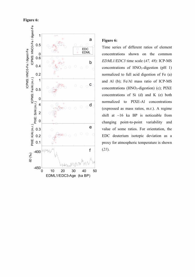
Figure 6:
Figure 6:
Time series of different ratios of element
concentrations shown on the common
EDML1/EDC3 time scale (47, 48): ICP-MS
concentrations of HNO3-digestion (pH 1)
normalized to full acid digestion of Fe (a)
and Al (b); Fe/Al mass ratio of ICP-MS
concentrations (HNO3-digestion) (c); PIXE
concentrations of Si (d) and K (e) both
normalized to PIXE-Al concentrations
(expressed as mass ratios, m.r.). A regime
shift at ~16 ka BP is noticeable from
changing point-to-point variability and
value of some ratios. For orientation, the
EDC deuterium isotopic deviation as a
proxy for atmospheric temperature is shown
(21).
0
0.5
1IC
PMS:
HN
O3-
Fe /
dige
st-F
e
a
EDCEDML
0.2
0.4
0.6
ICPM
S: H
NO
3-Fe
/ di
gest
-Fe
b
0
0.5
1
ICPM
S: F
e/Al
(m.r.
)
c
0
2
4
PIXE
: Si/A
l (m
.r.)
d
0.1
0.2
0.3
PIXE
: K/A
l (m
.r.)
e
0 10 20 30 40 50-450
-400
EDML1/EDC3-Age (ka BP)
δD (‰
) f


Acknowledgements
At the end, I would like to take the opportunity to thank a all the people, without
whose support I would not have finished this thesis.
At first, I would like to thank Prof. Heinz Miller for enabling this work and the
excellent work environment with outstanding opportunities: The network within
EPICA, the field campaign to Antarctica, the EPICA-meetings, the stay in Venice
and many more. Prof. Gerhard Bohrmann I would like to thank for being the
second evaluator. I also want to express my gratitude to Evangelisches Studienwerk
Villigst, e.V. for supporting me with funding.
Urs Ruth gave me the opportunity to do this thesis. With plenty of ideas he encour-
aged my work in the first two years, until he left for industry. After that Hubertus
Fischer took over and forced me to finish. Without him and his motivating optimism
it would have been a lot harder. Thank you very much for this.
Michael Kriews, Dorothee Dick and Ilse Stolting at the ICP-MS at AWI showed me
the way through the mystery of ICP-MS and helped me out whenever I was stuck.
Thank you!
Just as well during my stay at the university of Venice I got a lot of support from
the local people. Thank you for that and for the very nice stay at the laguna to
Prof. Carlo Barbante, Paolo Gabrielli, Vania Gaspari, Guilio Cozzi, Clara Turetta
and all the people around in the lab. Mille Grazie.
The field trip to Antarctica was a very exciting and unique experience. Thanks
to all the participants for making this journey so successful. Representatively, I
would like to thank Jens Kohler and Markus Weinand for helping me with all those
snowpits. Living in a field camp and being away from home for such a long time
is much easier, if there are nice people around. Thanks to Wolfgang Rack, Tobias
Bobel and Yannik Beer for sharing time and fun with me in Antarctica.
The biologists granted me asylum before the glaciology group got its own Coulter
Counter. Thanks to Uta Passow and Erika Allhusen for letting me use the instru-
ment and supporting me with their help.
Most of the time I spent in my office. Not only the most beautiful view in the
building, but also my very enjoyable colleagues Felix Fundel, Jochen Schmitt and
Veit Helm made working there a pleasure. I am especially grateful for the valuable
support in the final stage by Jochen.
199

Bibliography
A lot of my measurements I performed in the IC-Lab. Thanks to Birthe Twarloh
for nice company not only in the lab. Thanks to Barbara Delmonte and Reinhard
Winkler, who provided me with samples from the potential source areas.
Fernando Valero, thank you very much for your support and help with ice core boxes
and everything else. Thank you for the coffee and cake breaks and all the discussions
that made my life better.
Discussing the world and more was enjoyable in a lot of breaks in the Mensa, in
various Cafes and in front of the new espresso machine. Thanks to all the Glaciology
group for sharing this time with me.
During my time in Bremerhaven a lot of people meliorated my life. Since I cannot
possibly mention all the people who should be mentioned here, I just want to give
my special thanks representatively for all of them to Christina Morchner.
My parents always supported me during my studies and were always very interested
in my work. Thank you very much. Special thanks to Hermann for the valuable
comments on all, what I had to write and to Liese for always supporting me and
being just like she is.
200

Abbreviations
ACR Antarctic cold reversalCFA continuous flow analysisCC Coulter CounterCI chondriteCPP coarse particle percentageCSPC coordinate system spanned by the principal componentsCSREE coordinate system spanned by the rare earth elementsDML Dronning Maud LandEPICA-DML EPICA Dronning Maud LandEPICA European project of ice coring in AntarcticaFPP fine particle percentageHREE heavy rare earth element (Ho - Lu)IC ion chromatographyICP-MS inductively coupled plasma mass spectrometerICP-QP-MS inductively coupled plasma quadrupole mass spectrometerICP-SF-MS inductively coupled plasma sectorfield mass spectrometerICP-TOF-MS inductively coupled plasma time of flight mass spectrometerIPCC Intergovernmental Panel on Climate ChangeLREE heavy rare earth element (La - Nd)LS laser sensorMIS marine isotope stageMMD mean mass diameterMREE medium rare earth element (Sm - Dy)PAAS post archean Australian shellPC principcal componentPCA principcal component analysisPS polystyrenePSA potential source areaPTFE polytetrafluoroethylenREE rare earth elementsTE trace elementsUCC upper continental crust
201

E r k l a r u n g
Hiermit versichere ich, dass ich1. die Arbeit ohne unerlaubte fremde Hilfe angefertigt habe,2. keine anderen als die von mir angegebenen Quellen und Hilfsmittel benutzt habeund3. die den benutzten Werken wortlich oder inhaltlich entnommenen Stellen als solchekenntlich gemacht habe.
Bremerhaven, den 25.1.08
(Unterschrift)