Authorship Verification Authorship Identification Authorship Attribution Stylometry.

Source Code Authorship Attribution
A thesis submitted for the degree of
Doctor of Philosophy
Steven David Burrows B.App.Sc. (Hons.),
School of Computer Science and Information Technology,
College of Science, Engineering and Health,
RMIT University,
Melbourne, Victoria, Australia.
4th November, 2010


Declaration
I certify that except where due acknowledgement has been made, the work is that of the author alone;
the work has not been submitted previously, in whole or in part, to qualify forany other academic
award; the content of the thesis is the result of work which has been carried out since the official
commencement date of the approved research program; and, any editorial work, paid or unpaid,
carried out by a third party is acknowledged.
Steven David Burrows
School of Computer Science and Information Technology
RMIT University
4th November, 2010
i

ii

Acknowledgements
I first and foremost thank my PhD supervisors Dr. Alexandra Uitdenbogerd and Assoc. Prof. Andrew
Turpin for their ongoing encouragement, guidance, and feedback. Words alone cannot articulate my
gratitude. I am indebted to the support they have given me, for which I am truly thankful.
I also thank my previous PhD supervisors Prof. Justin Zobel and Dr. Saied Tahaghoghi for their
earlier supervision before moving on to other positions. I received an exceptional introduction to the
world of research from them during my honours degree.
I thank Upali Wickramasinghe for being my thesis reading buddy for exchanging thesis chapters
for feedback. The discussions we had were very valuable for improving the thesis.
I also thank Andrew Atkinson and David Burrows for taking the time to proof read a full draft of
my thesis. Thanks also goes to Michael Harris, Matthias Petri, Lida Ghahremanloo, Lorena Bando,
Jasbir Dhaliwal, Chris Hoobin, and Rahayu Hamid, for proof reading parts of my thesis.
I next thank the supportive environment of the School of Computer Science and Information
Technology at RMIT University, and in particular the Information Storage, Analysis and Retrieval
research group. The advice and support from staff and students both past and present has been
invaluable.
Finally, I thank my family and friends for their ongoing support and encouragement during my
time as a serial student. I needed all of you to keep me sane.
iii

iv

Credits
Portions of the material in this thesis have previously appeared in the followingpublications:
• S. Burrows and S. M. M. Tahaghoghi. Source code authorship attribution using n-grams. In
A. Spink, A. Turpin, and M. Wu, editors, Proceedings of the Twelfth Australasian Document
Computing Symposium, pages 32–39, Melbourne, Australia, December 2007. RMIT Univer-
sity.
• S. Burrows, A. L. Uitdenbogerd, and A. Turpin. Application of information retrieval techniques
for source code authorship attribution. In X. Zhou, H. Yokota, R. Kotagiri, and X. Lin, editors,
Proceedings of the Fourteenth International Conference on DatabaseSystems for Advanced
Applications, pages 699–713, Brisbane, Australia, April 2009. Springer.
• S. Burrows, A. L. Uitdenbogerd, and A. Turpin. Temporally robust software features for
authorship attribution. In T. Hey, E. Bertino, V. Getov, and L. Liu, editors, Proceedings of
the Thirty-Third Annual IEEE International Computer Software and Applications Conference,
pages 599–606, Seattle, Washington, July 2009. IEEE Computer Society Press.Best Student
Paper Award.
• S. Burrows, A. L. Uitdenbogerd, and A. Turpin. Authorship attribution of source code. In
submission.
This work was supported by the Australian Research Council and the Information Storage, Analysis
and Retrieval group within the School of Computer Science and InformationTechnology at RMIT
University.
The thesis was typeset using the LATEX 2ε document preparation system.
All trademarks are the property of their respective owners.
Note
Unless otherwise stated, all fractional results have been rounded to the displayed number of decimal
figures.
v

vi

Contents
Abstract 1
1 Introduction 3
1.1 Collections . . . . . . . . . . . . . . . . . . . . . . . . . . . . . . . . . . . . . . . 5
1.2 Benchmarking Previous Contributions . . . . . . . . . . . . . . . . . . . . . . .. . 6
1.3 Applying Information Retrieval . . . . . . . . . . . . . . . . . . . . . . . . . . . .. 6
1.4 Effectiveness Parameters . . . . . . . . . . . . . . . . . . . . . . . . . . . . . . . . 7
1.5 Improving Contributions in the Field . . . . . . . . . . . . . . . . . . . . . . . . . . 8
1.6 Thesis Structure . . . . . . . . . . . . . . . . . . . . . . . . . . . . . . . . . . . . .8
2 Background 11
2.1 Definitions . . . . . . . . . . . . . . . . . . . . . . . . . . . . . . . . . . . . . . . . 12
2.1.1 Computer Forensics . . . . . . . . . . . . . . . . . . . . . . . . . . . . . . 12
2.1.2 Software Forensics . . . . . . . . . . . . . . . . . . . . . . . . . . . . . . . 13
2.1.3 Authorship Attribution . . . . . . . . . . . . . . . . . . . . . . . . . . . . . 14
2.1.4 Related Areas . . . . . . . . . . . . . . . . . . . . . . . . . . . . . . . . . . 15
Plagiarism Detection . . . . . . . . . . . . . . . . . . . . . . . . . . . . . . 17
Near-Duplicate Detection . . . . . . . . . . . . . . . . . . . . . . . . . . . 22
Genre Classification . . . . . . . . . . . . . . . . . . . . . . . . . . . . . . 22
Stylochronometry . . . . . . . . . . . . . . . . . . . . . . . . . . . . . . . . 23
Phylogeny and Ontogeny . . . . . . . . . . . . . . . . . . . . . . . . . . . . 24
Identity Resolution . . . . . . . . . . . . . . . . . . . . . . . . . . . . . . . 24
2.2 Rationale . . . . . . . . . . . . . . . . . . . . . . . . . . . . . . . . . . . . . . . . 24
2.2.1 Academic Dishonesty . . . . . . . . . . . . . . . . . . . . . . . . . . . . . 24
2.2.2 Software Development Marketplaces . . . . . . . . . . . . . . . . . . . . . 27
2.2.3 Dispute, Litigation, and Theft . . . . . . . . . . . . . . . . . . . . . . . . . 27
vii

CONTENTS
2.2.4 Malicious Software Tracing . . . . . . . . . . . . . . . . . . . . . . . . . . 30
2.2.5 Pseudonymous Authors . . . . . . . . . . . . . . . . . . . . . . . . . . . . 31
2.2.6 Large Software Project Maintenance . . . . . . . . . . . . . . . . . . . . .. 31
2.2.7 Exploring Evolutionary History . . . . . . . . . . . . . . . . . . . . . . . . 31
2.2.8 Authorship Attribution Competitions . . . . . . . . . . . . . . . . . . . . . 32
2.3 Style . . . . . . . . . . . . . . . . . . . . . . . . . . . . . . . . . . . . . . . . . . . 32
2.3.1 Writing Style . . . . . . . . . . . . . . . . . . . . . . . . . . . . . . . . . . 33
2.3.2 Coding Style . . . . . . . . . . . . . . . . . . . . . . . . . . . . . . . . . . 33
2.3.3 Similarities and Differences between Writing and Coding Style . . . . . . . 34
2.3.4 Evolving Style . . . . . . . . . . . . . . . . . . . . . . . . . . . . . . . . . 34
2.3.5 Dishonest Style . . . . . . . . . . . . . . . . . . . . . . . . . . . . . . . . . 35
2.4 Measuring Style . . . . . . . . . . . . . . . . . . . . . . . . . . . . . . . . . . . . . 36
2.4.1 Metrics in the Literature . . . . . . . . . . . . . . . . . . . . . . . . . . . . 36
2.4.2 N-Grams . . . . . . . . . . . . . . . . . . . . . . . . . . . . . . . . . . . . 38
2.4.3 Watermarking . . . . . . . . . . . . . . . . . . . . . . . . . . . . . . . . . . 38
2.4.4 Automated Tools . . . . . . . . . . . . . . . . . . . . . . . . . . . . . . . . 38
2.4.5 Natural Language Measurements . . . . . . . . . . . . . . . . . . . . . . . 39
2.5 Information Retrieval Fundamentals . . . . . . . . . . . . . . . . . . . . . . . . .. 39
2.5.1 Search Engines . . . . . . . . . . . . . . . . . . . . . . . . . . . . . . . . . 40
2.5.2 Index Structures . . . . . . . . . . . . . . . . . . . . . . . . . . . . . . . . 42
2.5.3 Models for Query Matching . . . . . . . . . . . . . . . . . . . . . . . . . . 42
Cosine . . . . . . . . . . . . . . . . . . . . . . . . . . . . . . . . . . . . . 45
Okapi BM25 . . . . . . . . . . . . . . . . . . . . . . . . . . . . . . . . . . 45
Language Modelling with Dirichlet Smoothing . . . . . . . . . . . . . . . . 46
Pivoted Cosine . . . . . . . . . . . . . . . . . . . . . . . . . . . . . . . . . 47
2.5.4 Effectiveness Quantification . . . . . . . . . . . . . . . . . . . . . . . . . . 47
Precision and Recall . . . . . . . . . . . . . . . . . . . . . . . . . . . . . . 48
Reciprocal Rank and Mean Reciprocal Rank . . . . . . . . . . . . . . . . . 49
Average Precision and Mean Average Precision . . . . . . . . . . . . . . . .49
2.6 Machine Learning Fundamentals . . . . . . . . . . . . . . . . . . . . . . . . . . .. 49
2.6.1 Training and Testing . . . . . . . . . . . . . . . . . . . . . . . . . . . . . . 50
2.6.2 Cross Validation . . . . . . . . . . . . . . . . . . . . . . . . . . . . . . . . 50
2.6.3 Feature Selection . . . . . . . . . . . . . . . . . . . . . . . . . . . . . . . . 52
2.6.4 Discretisation . . . . . . . . . . . . . . . . . . . . . . . . . . . . . . . . . . 52
viii
CONTENTS
2.7 Classification Algorithms . . . . . . . . . . . . . . . . . . . . . . . . . . . . . . . . 53
2.7.1 Decision Trees . . . . . . . . . . . . . . . . . . . . . . . . . . . . . . . . . 53
2.7.2 Nearest Neighbour Methods . . . . . . . . . . . . . . . . . . . . . . . . . . 53
2.7.3 Neural Networks . . . . . . . . . . . . . . . . . . . . . . . . . . . . . . . . 54
2.7.4 Case-Based Reasoning . . . . . . . . . . . . . . . . . . . . . . . . . . . . . 54
2.7.5 Discriminant Analysis . . . . . . . . . . . . . . . . . . . . . . . . . . . . . 54
2.7.6 Regression Analysis . . . . . . . . . . . . . . . . . . . . . . . . . . . . . . 55
2.7.7 Support Vector Machines . . . . . . . . . . . . . . . . . . . . . . . . . . . . 55
2.7.8 Voting Feature Intervals . . . . . . . . . . . . . . . . . . . . . . . . . . . . 55
2.7.9 Bayesian Networks . . . . . . . . . . . . . . . . . . . . . . . . . . . . . . . 56
2.7.10 Simplified Profile Intersection . . . . . . . . . . . . . . . . . . . . . . . . . 56
2.8 Summary . . . . . . . . . . . . . . . . . . . . . . . . . . . . . . . . . . . . . . . . 56
3 Collections 57
3.1 Important Criteria for Collection Construction . . . . . . . . . . . . . . . . . . .. . 58
3.2 Collections in the Thesis . . . . . . . . . . . . . . . . . . . . . . . . . . . . . . . . 60
3.2.1 Collection Coll-A . . . . . . . . . . . . . . . . . . . . . . . . . . . . . . . 60
3.2.2 Collection Coll-T . . . . . . . . . . . . . . . . . . . . . . . . . . . . . . . 63
3.2.3 Collection Coll-P . . . . . . . . . . . . . . . . . . . . . . . . . . . . . . . 65
3.2.4 Collection Coll-J . . . . . . . . . . . . . . . . . . . . . . . . . . . . . . . . 67
3.2.5 Collections Coll-PO and Coll-JO . . . . . . . . . . . . . . . . . . . . . . . 67
3.3 Analysis of the Collections . . . . . . . . . . . . . . . . . . . . . . . . . . . . . . . 67
3.4 Comparison of Our Collections to Collections in Previous Work . . . . . . . . .. . 70
3.5 Roles of the Collections . . . . . . . . . . . . . . . . . . . . . . . . . . . . . . . . . 74
3.6 Availability of the Collections . . . . . . . . . . . . . . . . . . . . . . . . . . . . . 75
3.7 Summary . . . . . . . . . . . . . . . . . . . . . . . . . . . . . . . . . . . . . . . . 76
4 Benchmarking Previous Contributions 77
4.1 Related Areas . . . . . . . . . . . . . . . . . . . . . . . . . . . . . . . . . . . . . . 77
4.1.1 Plagiarism Detection . . . . . . . . . . . . . . . . . . . . . . . . . . . . . . 78
Natural Language Plagiarism Detection . . . . . . . . . . . . . . . . . . . . 78
Metric-Based Source Code Plagiarism Detection . . . . . . . . . . . . . . . 80
Structure-Based Source Code Plagiarism Detection . . . . . . . . . . . . . . 81
4.1.2 Genre Classification . . . . . . . . . . . . . . . . . . . . . . . . . . . . . . 84
4.2 Natural Language Authorship Attribution . . . . . . . . . . . . . . . . . . . . .. . 85
ix

CONTENTS
4.3 Source Code Authorship Attribution Contributions . . . . . . . . . . . . . . . .. . 90
4.3.1 Krsul and Spafford . . . . . . . . . . . . . . . . . . . . . . . . . . . . . . . 92
4.3.2 MacDonell et al. . . . . . . . . . . . . . . . . . . . . . . . . . . . . . . . . 93
4.3.3 Ding and Samadzadeh . . . . . . . . . . . . . . . . . . . . . . . . . . . . . 93
4.3.4 Frantzeskou et al. . . . . . . . . . . . . . . . . . . . . . . . . . . . . . . . . 94
4.3.5 Kothari et al. . . . . . . . . . . . . . . . . . . . . . . . . . . . . . . . . . . 96
4.3.6 Lange and Mancoridis . . . . . . . . . . . . . . . . . . . . . . . . . . . . . 98
4.3.7 Elenbogen and Seliya . . . . . . . . . . . . . . . . . . . . . . . . . . . . . . 99
4.3.8 Shevertalov et al. . . . . . . . . . . . . . . . . . . . . . . . . . . . . . . . . 99
4.3.9 Other Work . . . . . . . . . . . . . . . . . . . . . . . . . . . . . . . . . . . 100
4.3.10 Comparison of Published Results . . . . . . . . . . . . . . . . . . . . . . . 100
4.4 Benchmarking Methodology . . . . . . . . . . . . . . . . . . . . . . . . . . . . . .102
4.4.1 Reimplementation of Frantzeskou Approach . . . . . . . . . . . . . . . . . 102
4.4.2 Reimplementation of Metric-Based Approaches with Weka . . . . . . . . . . 102
4.4.3 Methodology Common to All Approaches . . . . . . . . . . . . . . . . . . . 104
4.5 Benchmarking Results . . . . . . . . . . . . . . . . . . . . . . . . . . . . . . . . . 106
4.6 Summary . . . . . . . . . . . . . . . . . . . . . . . . . . . . . . . . . . . . . . . . 106
5 Applying Information Retrieval 109
5.1 Methodology . . . . . . . . . . . . . . . . . . . . . . . . . . . . . . . . . . . . . . 110
5.1.1 Collection Construction and Anonymisation . . . . . . . . . . . . . . . . . . 110
5.1.2 Tokenisation . . . . . . . . . . . . . . . . . . . . . . . . . . . . . . . . . . 111
5.1.3 N-Gram Construction . . . . . . . . . . . . . . . . . . . . . . . . . . . . . . 112
5.1.4 Indexing . . . . . . . . . . . . . . . . . . . . . . . . . . . . . . . . . . . . 113
5.1.5 Querying . . . . . . . . . . . . . . . . . . . . . . . . . . . . . . . . . . . . 113
5.1.6 Measuring Effectiveness . . . . . . . . . . . . . . . . . . . . . . . . . . . . 113
5.2 N-Gram Size and Similarity Measure . . . . . . . . . . . . . . . . . . . . . . . . . .118
5.3 Selecting Source Code Features . . . . . . . . . . . . . . . . . . . . . . . . . .. . 122
5.3.1 Backwards Feature Selection . . . . . . . . . . . . . . . . . . . . . . . . . . 122
5.3.2 Evaluating Feature Classes from the Literature . . . . . . . . . . . . . . . .122
5.4 Classification . . . . . . . . . . . . . . . . . . . . . . . . . . . . . . . . . . . . . . 129
5.4.1 Overall Results . . . . . . . . . . . . . . . . . . . . . . . . . . . . . . . . . 129
5.4.2 Comparing Accuracy to the Reimplemented Work . . . . . . . . . . . . . . 131
5.5 Managing the Number of Indexes . . . . . . . . . . . . . . . . . . . . . . . . . .. 132
x
CONTENTS
5.6 Summary . . . . . . . . . . . . . . . . . . . . . . . . . . . . . . . . . . . . . . . . 134
6 Effectiveness Parameters 135
6.1 Problem Size . . . . . . . . . . . . . . . . . . . . . . . . . . . . . . . . . . . . . . 135
6.1.1 Number of Authors . . . . . . . . . . . . . . . . . . . . . . . . . . . . . . . 136
6.1.2 Number of Samples per Author . . . . . . . . . . . . . . . . . . . . . . . . 137
6.2 Sample Length . . . . . . . . . . . . . . . . . . . . . . . . . . . . . . . . . . . . . 140
6.3 Strength of Style . . . . . . . . . . . . . . . . . . . . . . . . . . . . . . . . . . . . 142
6.3.1 Analysis of Outlier Results . . . . . . . . . . . . . . . . . . . . . . . . . . . 142
6.3.2 Automation of Style Analysis . . . . . . . . . . . . . . . . . . . . . . . . . 146
6.4 Timestamps . . . . . . . . . . . . . . . . . . . . . . . . . . . . . . . . . . . . . . . 147
6.4.1 Timestamp Collection Methodology . . . . . . . . . . . . . . . . . . . . . . 149
6.4.2 Timestamp Collection Baseline Results . . . . . . . . . . . . . . . . . . . . 150
6.5 Using Timestamps to Explore Topical and Temporal Effects . . . . . . . . . . . . . . 154
6.5.1 Ignoring Futuristic Matches . . . . . . . . . . . . . . . . . . . . . . . . . . 155
Managing the Number of Indexes Again . . . . . . . . . . . . . . . . . . . . 156
6.5.2 Topical Matches . . . . . . . . . . . . . . . . . . . . . . . . . . . . . . . . 156
6.5.3 Temporal Matches . . . . . . . . . . . . . . . . . . . . . . . . . . . . . . . 159
6.5.4 Semester-Based Matches . . . . . . . . . . . . . . . . . . . . . . . . . . . . 159
6.5.5 Other Types of Matches . . . . . . . . . . . . . . . . . . . . . . . . . . . . 162
6.6 Using Entropy to Identify Highly Discriminating Features . . . . . . . . . . . . .. 162
6.7 Improving Accuracy with Highly Discriminating Features . . . . . . . . . . . . .. 168
6.8 Summary . . . . . . . . . . . . . . . . . . . . . . . . . . . . . . . . . . . . . . . . 171
7 Improving Contributions in the Field 173
7.1 Overall Results for the Information Retrieval Approach . . . . . . . . . .. . . . . . 173
7.2 Improving N-Gram Approaches . . . . . . . . . . . . . . . . . . . . . . . . . .. . 175
7.2.1 Profile Length . . . . . . . . . . . . . . . . . . . . . . . . . . . . . . . . . 177
7.2.2 N-Gram Size . . . . . . . . . . . . . . . . . . . . . . . . . . . . . . . . . . 179
7.2.3 Anonymisation Effects . . . . . . . . . . . . . . . . . . . . . . . . . . . . . 179
7.2.4 N-Gram Composition . . . . . . . . . . . . . . . . . . . . . . . . . . . . . 181
7.3 Improving Metric-Based Approaches . . . . . . . . . . . . . . . . . . . . . .. . . . 183
7.3.1 Evaluating Combinations of Metrics and Classifiers . . . . . . . . . . . . . . 183
7.3.2 Machine Learning with N-Gram Features . . . . . . . . . . . . . . . . . . . 187
7.4 Summary of Results . . . . . . . . . . . . . . . . . . . . . . . . . . . . . . . . . . . 189
xi

CONTENTS
7.5 Summary . . . . . . . . . . . . . . . . . . . . . . . . . . . . . . . . . . . . . . . . 195
8 Conclusions 197
8.1 Collections . . . . . . . . . . . . . . . . . . . . . . . . . . . . . . . . . . . . . . . 197
8.2 Benchmarking Previous Contributions . . . . . . . . . . . . . . . . . . . . . . .. . 198
8.3 Applying Information Retrieval . . . . . . . . . . . . . . . . . . . . . . . . . . . .. 198
8.4 Effectiveness Parameters . . . . . . . . . . . . . . . . . . . . . . . . . . . . . . . . 199
8.5 Improving Contributions in the Field . . . . . . . . . . . . . . . . . . . . . . . . . . 200
8.6 Future Work . . . . . . . . . . . . . . . . . . . . . . . . . . . . . . . . . . . . . . . 201
8.6.1 Information Retrieval Approach . . . . . . . . . . . . . . . . . . . . . . . . 201
8.6.2 Frantzeskou Approach . . . . . . . . . . . . . . . . . . . . . . . . . . . . . 202
8.6.3 Metric-Based Approaches with Machine Learning . . . . . . . . . . . . .. 203
8.6.4 Related Problems . . . . . . . . . . . . . . . . . . . . . . . . . . . . . . . . 203
8.7 Summary . . . . . . . . . . . . . . . . . . . . . . . . . . . . . . . . . . . . . . . . 204
A Glossary 207
A.1 Authorship Attribution Glossary . . . . . . . . . . . . . . . . . . . . . . . . . . . .207
A.2 Information Retrieval Glossary . . . . . . . . . . . . . . . . . . . . . . . . . . .. . 208
A.3 Machine Learning Glossary . . . . . . . . . . . . . . . . . . . . . . . . . . . . .. . 209
B Reconstruction of Freelance Collections 211
C Features from the Literature 219
D Programming Language Feature Tables 229
References 235
xii

List of Figures
2.1 Authorship Attribution . . . . . . . . . . . . . . . . . . . . . . . . . . . . . . . . . 16
2.2 Authorship Mismatch . . . . . . . . . . . . . . . . . . . . . . . . . . . . . . . . . . 19
2.3 Co-derivative Match . . . . . . . . . . . . . . . . . . . . . . . . . . . . . . . . .. 20
2.4 RentACoder Web Site . . . . . . . . . . . . . . . . . . . . . . . . . . . . . . . . . . 28
2.5 Centralised Search Engine Architecture . . . . . . . . . . . . . . . . . . . . .. . . 40
2.6 Inverted Index . . . . . . . . . . . . . . . . . . . . . . . . . . . . . . . . . . . . .. 43
2.7 Precision and Recall . . . . . . . . . . . . . . . . . . . . . . . . . . . . . . . . . .48
2.8 Six-Fold Cross Validation . . . . . . . . . . . . . . . . . . . . . . . . . . . . . . . .51
2.9 Ten-Fold Cross Validation . . . . . . . . . . . . . . . . . . . . . . . . . . . . . . .52
3.1 Turnin Submission Terms . . . . . . . . . . . . . . . . . . . . . . . . . . . . . . . . 62
3.2 Order of the Six Tasks from the Temporal Collection . . . . . . . . . . . . . .. . . 63
3.3 Number of Samples per Author in Our Collections . . . . . . . . . . . . . . . . . .71
3.4 Number of Lines of Code per Sample in Our Collections . . . . . . . . . . . . . .. 72
4.1 JPlag Interface . . . . . . . . . . . . . . . . . . . . . . . . . . . . . . . . . . . . .83
4.2 General Source Code Authorship Attribution System Structure . . . . . .. . . . . . 91
4.3 Frequency of Byte-Level 4-Grams in Author Profiles . . . . . . . . . . .. . . . . . 97
4.4 Baseline Reimplementation Results . . . . . . . . . . . . . . . . . . . . . . . . . . 107
5.1 Methodology Step 2: Collection Construction and Anonymisation . . . . . . . .. . 111
5.2 Methodology Step 3: Tokenisation . . . . . . . . . . . . . . . . . . . . . . . . . .. 112
5.3 Methodology Step 4: N-Gram Construction . . . . . . . . . . . . . . . . . . . .. . 114
5.4 Methodology Step 5: Indexing . . . . . . . . . . . . . . . . . . . . . . . . . . . .. 115
5.5 Methodology Step 6: Querying . . . . . . . . . . . . . . . . . . . . . . . . . . . .. 116
5.6 Methodology Step 7: Measuring Effectiveness . . . . . . . . . . . . . . . . . . . . . 117
xiii

LIST OF FIGURES
5.7 Sunflower Plot of Results for Our Approach . . . . . . . . . . . . . . . . .. . . . . 121
5.8 Six Feature Classes in Marked-Up Source Code . . . . . . . . . . . . . . .. . . . . 124
5.9 Token Volume versus MRR for Our Approach . . . . . . . . . . . . . . . . .. . . . 127
5.10 Token Volume versus MRR for Our Approach (Expanded) . . . . . .. . . . . . . . 128
5.11 Our Approach compared with Baseline Reimplementation Results . . . . . . . .. . 133
6.1 Query Length versus Accuracy for Our Approach . . . . . . . . . . .. . . . . . . . 141
6.2 Lines of Code versus Accuracy for Our Approach . . . . . . . . . . .. . . . . . . . 143
6.3 Style Score versus Accuracy for Our Approach . . . . . . . . . . . . .. . . . . . . 148
6.4 Example Run using the Temporal Collection . . . . . . . . . . . . . . . . . . . . . .149
6.5 Temporal Collection Accuracy Results for Six Tasks . . . . . . . . . . . . .. . . . 151
6.6 Omitting Results Variation 1: Ignoring Futuristic Matches . . . . . . . . . . . . . .157
6.7 Omitting Results Variation 2: Topical Matches . . . . . . . . . . . . . . . . . . . . .158
6.8 Omitting Results Variation 3: Temporal Matches . . . . . . . . . . . . . . . . . . . 160
6.9 Omitting Results Variation 4: Semester-Based Matches . . . . . . . . . . . . . . .. 161
6.10 Omitting Results Variation 5: Futuristic Assignment-Based Matches . . . . . . .. . 163
6.11 Omitting Results Variation 6: Futuristic Semester-Based Matches . . . . . . . .. . 164
6.12 Inefficient C Code that Distorted Entropy Calculations . . . . . . . . . . . . . . . . 167
6.13 Equivalent Source Code using Arrays or Pointers . . . . . . . . . . .. . . . . . . . 167
6.14 Use of Parentheses and Carriage Returns . . . . . . . . . . . . . . . . .. . . . . . . 169
7.1 Comparison of Previous Results to Our Results for All Collections . . . . . .. . . . 176
7.2 Varying Profile Length for Frantzeskou Approach . . . . . . . . . . . .. . . . . . . 178
7.3 Effective N-Gram Lengths for N-Gram Approaches . . . . . . . . . . . . . . .. . . 180
7.4 Comparison of Feature and Byte N-Grams for Our Work . . . . . . . . . . .. . . . 181
7.5 Comparison of Feature and Byte N-Grams for Frantzeskou Work . . . .. . . . . . . 182
7.6 Summary Results for Classifiers and Feature Sets . . . . . . . . . . . . . . . .. . . 185
7.7 Accuracy Scores using Normalised Token Count Features . . . . . . .. . . . . . . . 188
7.8 Accuracy Scores using Normalised N-Gram Count Features . . . . . .. . . . . . . 190
7.9 Comparison of Leading Approaches . . . . . . . . . . . . . . . . . . . . . . .. . . 191
B.1 Planet Source Code Collection Construction Step 1 . . . . . . . . . . . . . . .. . . 212
B.2 Planet Source Code Collection Construction Step 2 . . . . . . . . . . . . . . .. . . 213
B.3 Planet Source Code Collection Construction Step 3 . . . . . . . . . . . . . . .. . . 214
B.4 Planet Source Code Collection Construction Step 4 . . . . . . . . . . . . . . .. . . 215
xiv
LIST OF FIGURES
B.5 Planet Source Code Collection Construction Step 5 . . . . . . . . . . . . . . .. . . 216
B.6 Planet Source Code Collection Construction Step 6 . . . . . . . . . . . . . . .. . . 217
xv

LIST OF FIGURES
xvi

List of Tables
2.1 Code Sharing Web Sites . . . . . . . . . . . . . . . . . . . . . . . . . . . . . . . . 26
3.1 Average Lines of Code for Each Task in the Temporal Collection . . . . .. . . . . . 64
3.2 Properties of the Collections . . . . . . . . . . . . . . . . . . . . . . . . . . . . . .69
3.3 Comparison of the Collections . . . . . . . . . . . . . . . . . . . . . . . . . . . . . 73
4.1 Comparison of Results from the Literature . . . . . . . . . . . . . . . . . . . . .. . 101
4.2 Weka Classifiers Used to Reimplement the Previous Work . . . . . . . . . . . .. . 104
5.1 N-Gram and Similarity Measure Results for Our Approach . . . . . . . . . .. . . . 119
5.2 Feature and Token Statistics for Collection Coll-A . . . . . . . . . . . . . . . . . . 125
5.3 Accuracy Scores for the Six Feature Classes . . . . . . . . . . . . . . . .. . . . . . 126
5.4 Worked Examples for Three Accuracy Metrics . . . . . . . . . . . . . . . .. . . . . 130
5.5 Accuracy Results using the Three Accuracy Metrics . . . . . . . . . . . .. . . . . . 131
6.1 Results for Modifying the Number of Authors . . . . . . . . . . . . . . . . . . .. . 136
6.2 Two-Class Results for Modifying the Number of Samples per Author . . . .. . . . 138
6.3 Ten-Class Results for Modifying the Number of Samples per Author . . . .. . . . . 139
6.4 Token Statistics for All Collections . . . . . . . . . . . . . . . . . . . . . . . . . . .140
6.5 Criteria for Measuring Stylistic Strength . . . . . . . . . . . . . . . . . . . . . . .. 144
6.6 Stylistic Strength Scores for Four Outlier Authors . . . . . . . . . . . . . . . .. . . 145
6.7 Confusion Matrices for Temporal Collection Accuracy Results . . . . . .. . . . . . 152
6.8 Pearson’s Chi-Squared Tests for Temporal Collection Results . . . . .. . . . . . . . 153
6.9 Entropy between Task Samples and Author Samples . . . . . . . . . . . . . . .. . 166
6.10 Entropy of White Space Features . . . . . . . . . . . . . . . . . . . . . . . . .. . . 170
7.1 Accuracy Scores for Our Approach . . . . . . . . . . . . . . . . . . . . .. . . . . . 175
xvii

LIST OF TABLES
7.2 Byte-Level N-Gram Statistics for All Collections . . . . . . . . . . . . . . . . .. . 177
7.3 Accuracy Score Changes for Original Collections . . . . . . . . . . . . .. . . . . . 180
7.4 Okapi BM25 and SPI Results using Feature and Byte N-grams . . . . . . .. . . . . 183
7.5 Average Metric-Based System Performance for All Classifiers . . . .. . . . . . . . 186
7.6 Average Metric-Based System Performance for All Feature Sets . . .. . . . . . . . 187
7.7 N-Gram Token Statistics for All Collections . . . . . . . . . . . . . . . . . . . . .. 187
7.8 Summary of Results for Whole Thesis . . . . . . . . . . . . . . . . . . . . . . . . .193
C.1 Feature Sets from the Previous Work . . . . . . . . . . . . . . . . . . . . . . .. . . 221
D.1 C Language Operators and Keywords . . . . . . . . . . . . . . . . . . . . .. . . . 230
D.2 C++ Language Operators and Keywords . . . . . . . . . . . . . . . . . . . . . . . .231
D.3 Java Language Operators and Keywords . . . . . . . . . . . . . . . . . .. . . . . . 232
D.4 C Language Features for Six Feature Classes . . . . . . . . . . . . . . . .. . . . . 233
D.5 C Language Function Words . . . . . . . . . . . . . . . . . . . . . . . . . . . . .. 234
xviii
Abstract
To attribute authorship means to identify the true author among many candidates for samples of
work of unknown or contentious authorship. Authorship attribution is a prolific research area for
natural language, but much less so for source code, with eight other research groups having published
empirical results concerning the accuracy of their approaches to date. Authorship attribution of source
code is the focus of this thesis.
We first review, reimplement, and benchmark all existing published methods to establish a con-
sistent set of accuracy scores. This is done using four newly constructed and significant source code
collections comprising samples from academic sources, freelance sources, and multiple programming
languages. The collections developed are the most comprehensive to datein the field.
We then propose a novel information retrieval method for source code authorship attribution. In
this method, source code features from the collection samples are tokenised, converted into n-grams,
and indexed for stylistic comparison to query samples using the Okapi BM25 similarity measure.
Authorship of the top ranked sample is used to classify authorship of each query, and the proportion
of times that this is correct determines overall accuracy. The results showthat this approach is more
accurate than the best approach from the previous work for three of the four collections.
The accuracy of the new method is then explored in the context of author style evolving over time,
by experimenting with a collection of student programming assignments that spans three semesters
with established relative timestamps. We find that it takes one full semester for individual coding
styles to stabilise, which is essential knowledge for ongoing authorship attribution studies and quality
control in general.
We conclude the research by extending both the new information retrieval method and previous
methods to provide a complete set of benchmarks for advancing the field. In the final evaluation,
we show that the n-gram approaches are leading the field, with accuracyscores for some collections
around 90% for a one-in-ten classification problem.
1

2

Chapter 1
Introduction
The topic of this thesis is inherently related to the analysis of writing style. Writing style of any
individual begins to develop from an early age and continues to develop throughout life. Each writ-
ing style is different and is influenced by many factors, such as schooling, family, and community.
Therefore, it should be possible to determine the author of an unattributed piece of work based on the
writing style of the candidates. This is known asauthorship attribution.
A common misconception is that authorship attribution will fail if writing style is strongly in-
fluenced. Moreover, interpretation of results of authorship techniquessuch as thecusumtechnique
has at times brought the field under dispute, as it has been claimed that this technique is “extremely
subjective and is open to ad hoc interpretation” [Holmes and Tweedie, 1995]. It might be thought
that a class of students being taught by the same English teacher for an extended period of time would
adopt the same writing style. This is unlikely to cause authorship attribution to fail,since there are
sufficient components in writing that are always open to personal choice.
Writing elements that may offer little personal choice are those documented in style guides such
as the “Publication Manual of the American Psychological Association” by the American Psycho-
logical Association [2009] and “Writing for Computer Science” by Zobel [2004b]. These books
cover rules that are widely accepted concerning punctuation, citation, capitalisation, abbreviations,
and even preferred spelling. A specific example that was addressed in the development of this thesis
concerned when numbers should be expressed as numerals or words.
Many elements of writing style still remain open to personal choice, however.Perhaps the most
obvious example is word choice. It is always the decision of the individual concerning the words
that make up each sentence, as there are a multitude of ways that each idea can be expressed. For
example, during the development of this thesis, the frequent use of the word “contribution” stood
out as a preference, whereas others might have preferred to use alternatives more frequently such as
3

CHAPTER 1. INTRODUCTION
“approach”, “research”, or “work”.
At the individual word level, the basic restriction is spelling rules. Preference can also be exhib-
ited at the phrase level, providing that grammatical correctness is maintained.Such phrases could be
as short as word pairs or as long as full sentences. Again referring tothe development of this thesis
as an example, it was noted that the author had strong preference to use certain phrases for sentence
beginnings, and work was undertaken to introduce more variety.
Word-level and phrase-level preferences may be particularly obvious when mistakes are made.
For example, particular spelling errors or unusual grammatical structuresmay also strongly demon-
strate personal traits. Moreover, general preferences concerning various parts of speech such as
nouns, verbs and conjunctions can indicate stylistic preferences. These preferences may be observed
statistically at the word level, or by observing common patterns at the phrase level, demonstrating
preferred language constructs.
Writing style, preference, and idiom, are not restricted to natural language writing as discussed
above, but also feature in other forms of “writing” such as computer language source code. It might
be thought that programming languages are too prescriptive for individual style to be demonstrated
in source code, since coding standards provide guidelines for aspectsof programming style such as
comments, layout, naming conventions, source file organisation, and general readability. Moreover,
a program must follow rigid syntactic rules to compile.
Despite the need to satisfy coding standards and compilation rules, there is much freedom and
choice that goes into writing software. Using the choice of standard libraryfunctions as an example,
there are usually many ways to process standard data input and to output data to files and the con-
sole. Another example is interchangable looping and branching constructs, such as “if/else” versus
“switch/case”, and “for” versus “while” versus “do-while” in C-like languages. Yet another example
is the use of compound statements, such as replacing “a = a + b” with “ a += b”. Perhaps the most
freedom is given with the use of white space for indentation, the placement of curly braces for code
blocks, and commenting.
There are two clear areas of previous authorship attribution research,for natural language and
source code respectively. Natural language authorship attribution is a mature area of research with
many publications. For example, the seventy-four contributions summarised by Koppel et al. [2009]
spanning 1887 to 2008 comprise many of them. Conversely, the firstsource code authorship attri-
butionempirical contribution was presented by Krsul [1994], and there are only eight prior research
groups who have published empirical results in this area to the best of our knowledge, apart from our
own work.1
1Our comprehensive literature review comprised the use of search engines, digital libraries, and resource bibliographies.
4

1.1. COLLECTIONS
Authorship attribution can help solve many practical and adversarial problems. The following
types of questions are typical examples of investigations requiring sourcecode authorship attribution,
whether they be in academia, industry, or in general:
1. Who was the original author in this pair of plagiarised programming assignments?
2. Who was responsible for writing this defective code?
3. Who was the author of this particular computer virus?
4. Who wrote this unattributed software?
These questions are all authorship attribution problems as they have a “who” component. Other
questions that belong to related topics concern “when”, “where”, “why”, and “how many”, and are
generally beyond the scope of authorship attribution and hence this thesis.
This thesis offers several new contributions in the field of source code authorship attribution,
which enables questions such as the above four to be better answered. In Sections 1.1 to 1.5, we
review the research problems that we address in Chapters 3 to 7.
1.1 Collections
Following the thesis background material in Chapter 2, in Chapter 3 we explainthat the first step in
any authorship attribution study is the construction of suitable collections. However, care must be
taken concerning the criteria that should be used to construct such collections. For example, we want
to ensure that our work is applicable to a variety of problem settings, thus it isimportant that our
collections represent multiple programming languages, and come from a variety of sources. The first
contribution of this thesis is the presentation of our list of eleven criteria for collection construction,
based on our review of the previous work. These criteria are used when documenting our collections
and those in previous work.
We next describe the construction of four large source code collections, which meet our criteria
as best as possible, using data from a school student assignment submission archive and a code
sharing web site. When comparing the properties of our collections to those of the previous research
groups, we show that our collections are the most comprehensive to date,making them the basis of
an excellent evaluation framework for advancing the field.
We conclude our review of the collections by sharing the location of our dataand instructions
for reproducing the collections. The data release comprises single-tokenand token-pair occurrence
statistics for the four collections, allowing others to reproduce parts of the work in this thesis, whilst
5

CHAPTER 1. INTRODUCTION
keeping the samples sufficiently scrambled to satisfy intellectual property and ethics requirements.
We also present a guide for reproducing the code-sharing web site collections, since we cannot pub-
lish the links due to the likelihood of some later becoming dead, or pass on the original samples due
to the terms and conditions of the web site.
1.2 Benchmarking Previous Contributions
Our contribution in Chapter 4 is to comprehensively review and reimplement previous work in the
field, and then benchmark the contributions against one another to establishthe leading methods.
We begin with a summary of the literature from related areas such as plagiarismdetection, genre
classification, and natural language authorship attribution, which servesto identify any key ideas
missing in the source code authorship attribution literature. The bulk of the literature review then
focuses on the collections, methods, and results from eight other research groups that have previously
published empirical results in source code authorship attribution.
Direct comparison of the published work is difficult, as few of the feature sets, similarity mea-
sures, and machine learning classification algorithms have been evaluated on the same collections. To
address this problem, we reimplement the previous work as closely as possible, to enable evaluation
using our collections. By doing this, we developed a consistent set of benchmarks for comparison to
our new information retrieval method for source code authorship attribution, introduced in Chapter 5.
The results to this point show that the coordinate matching approach using counts of byte-level
source code segments (orn-grams) [Frantzeskou et al., 2006a] is more effective than approaches
based on the use of software metrics as features, and machine learning algorithms for classification.
Coordinate matching achieves around 85% accuracy for a one-in-ten classification problem using
our largest collection from the code sharing web site, compared with the leading approach from the
software metric family of approaches, which achieves an accuracy of around 75%.
1.3 Applying Information Retrieval
In Chapter 5, we introduce an information retrieval approach to source code authorship attribution.
A clear conclusion from our literature review is that the use of n-grams is underexplored for source
code authorship attribution. Therefore, in our next contribution we aim to determine whether a new
implementation motivated by the information retrieval approach for source code plagiarism detection
by Burrows et al. [2006] is effective for source code authorship attribution. The method involves
indexing token-level n-grams of source code features (such as operators and keywords), so that we
can classify samples that are represented as queries to the index. The output returned from query
6

1.4. EFFECTIVENESS PARAMETERS
requests is a ranked list of samples, ordered from most relevant to leastrelevant based on stylistic
similarity. These lists can then be post-processed to identify the most likely author represented in the
index.
To implement the method described above, we need to establish optimal settings for the choice
of n-gram length, information retrieval similarity measure, feature set, and method for classifying
authorship of the query samples using the ranked lists. We initially use common information retrieval
metrics to gauge the quality of the returned ranked lists to make suitable decisionsfor the parameters
above. We identify that the Okapi BM25 similarity measure using token-level operator, keyword, and
white space features, is effective when combined in n-grams of lengthn= 6, which helps to preserve
the locality of the features.
We conclude Chapter 5 by exploring methods for making classification decisions using the ranked
lists. We evaluate a method that uses the top-returned sample from the rankedlist, and two other
methods that use the whole lists. We find that the method that uses only the top-returned sample is
the most effective. This finding suggests that authors commonly have some samples that are either
unhelpful or misleading for making authorship decisions, therefore not using the whole set seems to
be a good decision.
1.4 Effectiveness Parameters
After implementing and evaluating the information retrieval approach described above, in Chapter 6
we investigate how our method performs when manipulating key parameters thatwere kept constant
in the development of our approach, such as the number of authors, number of samples per author, and
sample length. Other variables investigated are the stylistic maturity of authors, and the timestamps
of samples. We expect these factors to affect the accuracy of our approach, and we explore each in
turn in separate experiments.
Previous source code authorship attribution research has assumed a stable feature set over time.
We investigate timing effects using a specially constructed collection of student assignments with
guaranteed relative timestamps established from a sequential chain of courses from our school. We
find that coding style is particularly unstable early in a programmers career.This finding suggests
that it takes one semester for programmers to develop a consistent coding style, which is interesting
for people who deal with source code quality control.
It is also unclear which individual features will be of most value for makingaccurate authorship
decisions, thus we explore their effect individually. We make use of entropy [Shannon, 1948] as a
measure of information content for this work. We find that white space playsan important role, and
7

CHAPTER 1. INTRODUCTION
adjust tokenisation to make best use of the white space features.
1.5 Improving Contributions in the Field
The goal of Chapters 5 and 6 is to develop and evaluate our information retrieval approach. Therefore,
the first results we present in Chapter 7 concern the overall performance of our approach compared
with the previous work. Results show that the Frantzeskou et al. [2006a]approach is around 85%
accurate when using our largest code sharing web site collection for the one-in-ten classification
problem, and we find that our approach has advanced the state-of-the-art to around 90% accuracy.
Moreover, when considering the full set of four collections, our approach is the most accurate for
three of the four collections.
In the remainder of Chapter 7, we describe refinements to the previous work by other researchers.
First, we consider the effect of exchanging the types of string patterns (n-grams) used in our work and
that of Frantzeskou et al. [2006a]. We find that these are interchangeable, however the Frantzeskou
et al. [2006a] method requires a different n-gram length and omission of the profile truncation step to
be more effective.
The accuracy scores for the remaining combinations of machine learning classification algorithms
and software metric feature sets are then evaluated. We find that the neural network and support
vector machine classifiers are the most effective classification algorithms, and that combining the
feature sets proposed by the previous research groups is more effective than the individual parts.
We also determine whether counts of n-gram occurrences normalised by sample length are effec-
tive when combined with the classification algorithms. We find that increased numbers of n-grams is
effective, but we do not establish a single recommendation, as we find that accuracy continues to in-
crease as the number of n-grams used increases up to the largest numberof n-grams tested. Given the
time required to complete this experiment, the recommendation for future work is to find a classifier
with the best compromise between accuracy and time.
The final section of this chapter includes a comparison of all results in a single table for all
combinations of feature set and classification method explored. These provide a comprehensive set
of benchmarks for future work, and clearly identify the methods attempted to date in source code
authorship attribution.
1.6 Thesis Structure
The remainder of this thesis is organised as follows. In Chapter 2, we provide background material
important for understanding the remainder of the thesis. This includes definitions, additional motiva-
8

1.6. THESIS STRUCTURE
tion, methods for measuring authorial style, and fundamentals of information retrieval and machine
learning. In Chapters 3 to 7, we present our contributions as outlined in Sections 1.1 to 1.5. We con-
clude in Chapter 8 with a summary of the outcomes and an agenda for future work. Four appendices
follow in Appendices A to D, which can be referred to when cited in the body of the thesis.
9

CHAPTER 1. INTRODUCTION
10
Chapter 2
Background
Authorship attribution in itself is not a new problem. There is a wealth of prior work in natural lan-
guage authorship attribution, and related areas such as plagiarism detection and genre classification.
There are also eight prior source code authorship attribution contributions with published empirical
results. Gaps in previous work have in part motivated the new research questions and contributions in
this thesis. This chapter covers all the necessary background material tolead into our contributions
presented in Chapters 3 to 7.
This chapter begins in Section 2.1, with definitions of and differentiations between the key prob-
lems areas in and related to our research. In Section 2.2, we motivate the importance and relevance of
the authorship attribution problem by covering practical application areas inacademia and industry.
We provide a discussion about writing style, coding style, and their differences, plus issues related to
evolving style due to the maturing of authors in Section 2.3, which forms a large part of Chapter 4.
Given the importance of style, in Section 2.4 we review several types of stylemeasurements and tech-
niques such as metrics, n-grams, and watermarks. In Section 2.5 we coverthe background material
essential to our information retrieval approach to source code authorship attribution introduced from
Chapter 5. In Section 2.6, we cover the machine learning background material essential for reimple-
menting the existing source code authorship attribution contributions in Chapter4, and our extensions
in Chapter 7. A series of machine learning classification algorithms are reviewed in Section 2.7 that
have appeared in previous source code authorship attribution contributions. Finally in Section 2.8,
we conclude this chapter by summarising the background work, highlighting the gaps in the previous
work, and by outlining our way forward to fill some of those gaps, with our contributions following
in Chapters 3 to 7.
11

CHAPTER 2. BACKGROUND
2.1 Definitions
Our definition of authorship attribution for this thesis is as follows:
Authorship attribution is the process of assigning authorship of an unattributed or con-
tentious sample of work to its correct author amongst a finite pool of authors.
There are many definitions of authorship attribution that are sometimes inconsistent with one
another. Therefore, we begin this section by defining the broader computer forensics and software
forensics fields that authorship attribution fits within. We then take care in reviewing subproblems,
alternative definitions, and synonyms that fall under the umbrella ofauthorship attribution, given the
inconsistency in the literature. Definitions of plagiarism detection, near-duplicate detection, genre
classification, stylochronometry, phylogeny, ontogeny, and identity resolution are provided in con-
clusion to this section, which should not be confused with authorship attribution.
2.1.1 Computer Forensics
Hall and Davis [2005] collated eight definitions ofcomputer forensicsin the literature including the
following by Abraham and de Vel [2002]:
“Computer forensics undertakes the post-mortem, or ‘after-the-event’ analysis of com-
puter crime. Of particular importance is the requirement to successfully narrow the po-
tentially large search space often presented to investigators of such crimes. This usually
involves some form(s) of guided processing of the data collected as evidence in order
to produce a shortlist of suspicious activities. Investigators can subsequently use this
shortlist to examine related evidence in more detail.”
Forensics in general concerns the collection of evidence to assist with legal proceedings. Hall
and Davis [2005] presented a computer forensics case concerning a road contractor who received se-
vere injury and disability after the heavy machinery he was operating surged forward after changing
gears. Hall and Davis [2005] investigated the roles of the contractor, machine supplier and manufac-
turer, hardware component designer and supplier, and the control system programmer to determine
legal liability for compensation purposes. This is a good example of a computerforensics case study,
as the investigation reviewed many types of legal artefacts including machinery, hardware, compo-
nents, data, design documentation, and source code.
12

2.1. DEFINITIONS
2.1.2 Software Forensics
Software forensicsis a sub-area of computer forensics dealing with programs and source code. In the
case study by Hall and Davis [2005] above, the software forensics component was the investigation
of the source code produced by the programmer. Another good example isthe floating-point error
that caused the $500 million Ariane rocket to explode in 1996 [Marc Jezequel and Meyer, 1997]. Hall
and Davis [2005] collated four definitions of software forensics in the literature, including the one
by Slade [2004]:
“Software forensics involves the analysis of evidence from program code itself. Program
code can be reviewed for evidence of activity, function, and intention, as well as evidence
of the software’s author.”
It is clear from this definition that the field of software forensics is also divided into several sub-
areas. For example, Gray et al. [1997] described software forensics as having four distinct areas:
author identification, author discrimination, author characterisation, and author intent determination.
Author identificationis the descriptor used by Gray et al. [1997] that we use to define authorship
attribution. That is, it deals with the problem of assigning authorship of a work sample based on other
available work samples of known authorship.
Author discriminationis the task of deciding whether one or several authors created a piece of
work. For example, this was used in the investigation of the malicious WANK and OILZ worms
that attacked numerous networks such as NASA in 1989 [Longstaff and Schultz, 1993], where there
were three suspected authors. Author discrimination is also related to collusion where students, for
example, sometimes work together inappropriately to complete assessment tasks[Bull et al., 2002].
Author characterisationuses programming style to gain an understanding of personal traits such
as educational background [Gray et al., 1997]. This area is also known as personality profiling [Kop-
pel et al., 2009]. Profiling practitioners aim to identify as much information as possible above and
beyond just authorship of a document, such as “demographic and psychological information” [Kop-
pel et al., 2009]. Krsul [1994] also noted the partial overlap with psychology.
Author intent determinationcan be used to find the reasons for software faults. Some software
faults may be simple oversights on behalf of programmers, but others may arise from malicious
intent. For example, a disgruntled employee may include a destructive statementthat is set to go
off after leaving their place of employment [Spafford, 1989a]. Similarly, a programmer may create
deliberately confusing code to enhance job security, as no-one else would have the skills or knowledge
to maintain it [Spinellis, 2009]. Identifying deliberate faults amongst accidental ones is critical in
maintaining business integrity.
13

CHAPTER 2. BACKGROUND
Author discrimination is not discussed in this thesis, as the scope is restricted tosingle-author
problems. We also do not focus on author characterisation or author intent determination problems,
as these are beyond the scope of this thesis. This leaves us with authorshipidentification — or
authorship attribution— as explored in this thesis.
2.1.3 Authorship Attribution
The authorship attribution definition given in Section 2.1 concerns a fixed set of candidate authors.
It is also possible that some candidate authors may be outside this set. Juola [2006] described these
two problems asclosed-classandopen-classrespectively. Juola [2006] described the closed-class
problem as: “given a particular sample of text known to be one of a set ofauthors, determine which
one”. The open class problem is: “given a particular sample of text believed to be one of a set of
authors, determine which one, if any” [Juola, 2006]. This second problem is much harder, as the
sample in question may not be represented in the collection at all. Interestingly,this problem remains
unattended in source code authorship attribution literature, as none of the previous contributions
reviewed in Chapter 4 have attempted this problem. This thesis also deals with the closed-class
problem, and the open-class problem remains as future work for sourcecode authorship attribution.
Juola [2006] also described a third problem, which does not fit under theopen-class and closed-
class definitions above; that is, all other problems that aim to infer more than just the author of the
program, such as the number of authors, and the background of the authors. This has already been
described as author discrimination and author characterisation by Gray etal. [1997] above, and Juola
[2006] referred to these areas asprofiling andstylometry. Moreover, the three problems described
by Juola [2006] have been grouped under the heading ofauthorship analysisby de Vel et al. [2001].
Stein et al. [2007] introducedauthorship identificationas their umbrella to cover their definitions
of authorship attributionandauthorship verification. Koppel and Schler [2004] and Koppel et al.
[2007] have also used authorship attribution and authorship verification definitions in the same way
as Stein et al. [2007] above, but without the authorship identification umbrella. Therefore we must
now distinguish authorship verification from authorship attribution.
In the Stein et al. [2007] report, the authorship attribution definition matches the closed-class
definition by Juola [2006] as discussed above. The definition for authorship verification by Stein
et al. [2007], however, is related to the open-class definition by Juola [2006], but has key differences
concerning the number of candidate authors in the problem. Stein et al. [2007] gave the following
definition for authorship verification: “one is given examples of the writing of a single author and is
asked to determine if given texts were or were not written by this author”. This definition essentially
asks the question: “Does this sample belong to this author?”, whereas the definition by Juola [2006]
14
2.1. DEFINITIONS
essentially asks: “Does this sample belong to any of these authors?” The definitions are similar as
they both include the possibility of the correct author being outside the candidate author set. The
only difference is the size of the author set: Stein and Meyer zu Eissen [2007] discussed a one-class
problem whereas Juola [2006] discussed a multi-class problem.
The above discussion regarding problem sizes clearly indicates that the difficulty of authorship
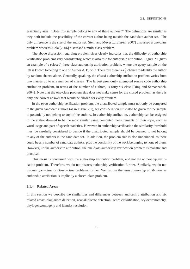
verification problems vary considerably, which is also true for authorshipattribution. Figure 2.1 gives
an example of a (closed) three-class authorship attribution problem, wherethe query sample on the
left is known to belong to one of Author A, B, or C. Therefore there is a13 chance to identify the author
by random chance alone. Generally speaking, theclosedauthorship attribution problem varies from
two classes up to any number of classes. The largest previously attempted source code authorship
attribution problem, in terms of the number of authors, is forty-six-class [Dingand Samadzadeh,
2004]. Note that the one-class problem size does not make sense for theclosed problem, as there is
only one correct answer that would be chosen for every problem.
In theopenauthorship verification problem, the unattributed sample must not only be compared
to the given candidate authors (as in Figure 2.1), but consideration must also be given for the sample
to potentially not belong to any of the authors. In authorship attribution, authorship can be assigned
to the author deemed to be the most similar using computed measurements of their style, such as
word usage and part of speech statistics. However, in authorship verification the similarity threshold
must be carefully considered to decide if the unattributed sample should be deemed to not belong
to any of the authors in the candidate set. In addition, the problem size is also unbounded, as there
could be any number of candidate authors, plus the possibility of the work belonging to none of them.
However, unlike authorship attribution, the one-class authorship verification problem is realistic and
practical.
This thesis is concerned with the authorship attribution problem, and not the authorship verifi-
cation problem. Therefore, we do not discuss authorship verification further. Similarly, we do not
discussopen-classor closed-classproblems further. We just use the termauthorship attribution, as
authorship attribution is implicitly a closed-class problem.
2.1.4 Related Areas
In this section we describe the similarities and differences between authorship attribution and six
related areas: plagiarism detection, near-duplicate detection, genre classification, stylochronometry,
phylogeny/ontogeny and identity resolution.
15

CHAPTER 2. BACKGROUND
Author AProfile A
Work A1 Work A2 Work A3
Author BProfile B
Work B3Work B2Work B1
Profile C Author C
Work C1 Work C2 Work C3
?
?
?
Work X
Author ?
Figure 2.1: A typical authorship attribution problem where an unattributed piece of work is beingassigned to one of three possible authors. With three candidate authors, this problem is described asthree-class. The circle, triangle, and square shapes in each work sample are metaphors for writingstyle. Therefore the unattributed work sample is likely to belong to Author C, given that both theunattributed sample and the Author C profile samples have many squares,which indicates similarstyle.
16

2.1. DEFINITIONS
Plagiarism Detection
RMIT University [2002] defined plagiarism as “the presentation of the work, idea, or creation of
another person as though it is your own”. iParadigms [2010] provide sixspecific examples of types
of plagiarism incidents:
• “Turning in someone else’s work as your own.
• Copying words or ideas from someone else without giving credit.
• Failing to put a quotation in quotation marks.
• Giving incorrect information about the source of a quotation.
• Changing words but copying the sentence structure of a source withoutgiving
credit.
• Copying so many words or ideas from a source that it makes up the majority of
your work, whether you give credit or not.”
To distinguish the difference between plagiarism detection and authorship attribution, we describe
plagiarism detection as being concerned with document content, and authorship attribution being
concerned with document style. To make this difference clear, we must review the three different
kinds of plagiarism problems in the literature: hermetic plagiarism detection, external plagiarism
detection, and intrinsic plagiarism detection.
Mozgovoy [2007] describedhermeticplagiarism detection systems as those that can process “lo-
cal collections of documents”. Therefore hermetic plagiarism detection refers to the inward-looking
or intracorpal problem. In practice, hermetic plagiarism detection involves the comparison of all sam-
ples from a class to one another in turn. Popular existing systems of this nature include JPlag [Prechelt
et al., 2002], MOSS [Bowyer and Hall, 1999], and Sherlock [Joy and Luck, 1999]. Therefore, in a
class ofsstudents there will be the following number of comparisons:
c=s−1∑
i=1
i (2.1)
Conversely,externalplagiarism detection [Grozea et al., 2009] is an outward-looking or extra-
corpal problem. This problem involves two collections of documents comprising a query set and a
reference set. The problem now is to determine whether there are any similarities between the sam-
ples in the query set and reference set. The query set can be the same collection of samples from a
class described above. However, there are really no restrictions on what can make up the reference
set. For example, a reference set could be a collection of student samplesfrom a previous offering
17

CHAPTER 2. BACKGROUND
of a course, where the aim is to determine whether previous students have passed work on to current
students. The reference set could also be documents obtained from external sources, such as the
Internet, to determine whether work has been obtained online.
Hermetic and external plagiarism detection is often combined. For example, theTurnitin aca-
demic integrity vendor [iParadigms, 2007b] conducts inward comparisons of batches of uploaded
assignments, and also compares these to their enormous database including books, journals and pre-
vious assignments. The exact algorithm is not known, as the inner-workings of the software are
commercial in confidence. However, Mozgovoy et al. [2005] noted somecollection statistics that
were available on the Turnitin web site around the time of their publication in November 2005; they
reported that the “database consists of over 4.5 billion pages which is updated daily with 40 million
pages”.
Authorship attribution can assist with academic and legal investigations involvinghermetic and
external plagiarism detection discussed above. For example, consider two types of plagiarism shown
in Figures 2.2 and 2.3: theauthorship mismatchand theco-derivative matchrespectively.
An authorship mismatchoccurs when one author obtains work by another. For example, Fig-
ure 2.2 demonstrates an incident where similar work samples were identified from Author B and
Author C. In this case, Author C is determined to be the receiving author, asthe style of the work
sample was found to be stylistically similar to previous work samples by Author B. With this fact es-
tablished, the investigation can continue to determine if the work was stolen or provided willingly to
Author C. Plagiarism detection software will regularly detect authorship mismatches provided both
samples are present in the collection. However, authorship attribution is required if the investigation
needs to differentiate the original author and the receiving author. This is critical in conducting aca-
demic integrity investigations and legal proceedings to determine blame and responsibility. Figure 2.2
demonstrates that if profiles of writing or coding style can be constructed from previous samples of
work by the authors in question, then the original and receiving authors can be differentiated.
The co-derivative matchscenario can arise when neither party has colluded with one another,
but instead independently obtained the same content from a third party. A plagiarism detection in-
vestigation can identify the similar content, but finding this may be coincidental if the authors were
working independently from one another. Figure 2.3 demonstrates a co-derivative match scenario,
where similar work has been identified between Author B and Author C. In thisexample, an author-
ship analysis could confirm that neither of the writing styles of samples Work Band Work C match
their typical work, represented in Profile B and Profile C. This means that the authorship mismatch
scenario shown in Figure 2.2 can be eliminated from any investigation.
18

2.1. DEFINITIONS
Work A
Profile A
Work C
Profile C
Work B
Profile B
Autho
rship
mism
atch
Mat
ch
Mat
ch
Author A Author B Author C
Figure 2.2: Author C has potentially plagiarised work belonging to Author B. That is, Work C wasprobably written by Author B, not Author C. This is an authorship profile mismatch. The circle,triangle and square shapes in each sample and profile are metaphors forwriting style. Therefore theWork C sample represents and authorship profile mismatch, since the stylematches the wrong profile.
19

CHAPTER 2. BACKGROUND
Work A
Profile A
Work C
Profile C
Work B
Profile B
Co−derivativematch
Mat
ch
Author A Author B Author C
Figure 2.3: Authors B and C have potentially plagiarised work from an external source. The Work Band Work C samples do not match previous examples of work by those authors in Profile B andProfile C. This is a co-derivative match. The circle, triangle, square, andhexagon shapes in eachsample and profile are metaphors for writing style. Therefore Work B and Work C samples representa co-derivative match, since their styles match one another but not the profiles.
20

2.1. DEFINITIONS
The authorship mismatch and co-derivative match scenarios in Figures 2.2 and 2.3 demonstrate
that plagiarism detection can only solvewithin-collectionproblems. For example, the authorship
mismatch problem may be undetectable with plagiarism detection techniques if one author was not
represented in the collection. This may occur if an outsider was hired to complete work. In this ex-
ample, an authorship analysis may still be able to determine that work was written by another party,
even if the identify of the other party remains unknown. Similarly, the co-derivative match problem
may also be undetectable with plagiarism detection techniques if only one co-derivative sample is
represented in the collection. This may occur if no other authors represented in the collection used
the derived work due to chance. Again, an authorship analysis may still beable to determine that the
work is not original. In summary, plagiarism detection techniques are very complementary with au-
thorship attribution techniques, which can help answer additional questionsthat plagiarism detection
techniques cannot.
Having reviewed hermetic and external plagiarism problems, we must now review the final prob-
lem: intrinsic plagiarism detection.Intrinsic plagiarism detection is a completely different problem to
hermetic and external plagiarism detection as it does not use a referencecollection [Meyer zu Eissen
and Stein, 2006]. Instead, the problem is to identify document chunks thatdemonstrate inconsistent
style with the remainder of the document, if any, to indicate potentially plagiarised components [Stein
and Meyer zu Eissen, 2007]. Therefore each document chunk is essentially treated as a separate and
potentially suspicious document in turn. This problem is synonymous with the open-class authorship
verification problem described previously in Section 2.1.3, with a key additional problem introduced
concerning the methods that should be used to determine the chunk boundaries.
The only plagiarism detection problem that has little overlap with authorship attribution is the
self plagiarismproblem [Collberg and Kobourov, 2005]. Self plagiarism detection can be applied
in academia to identify recycled and unoriginal publication content. It does not make sense to use
authorship attribution techniques for self plagiarism detection if the problem only concerns work
written by one author. However, there may be authorship discrimination applications for papers of
multiple authorship.
All of the plagiarism detection problems discussed above concern detectingincidents after they
have occurred. Other research inpreventativeplagiarism detection concerns avoidance through edu-
cation [Hamilton et al., 2004] and use of editors and integrated development environments to make
copy-and-paste incidents more difficult to commit [Vamplew and Dermoudy, 2005]. However, pre-
ventative plagiarism detection is unrelated to authorship attribution and is mentioned here for com-
pleteness only.
21

CHAPTER 2. BACKGROUND
Near-Duplicate Detection
Near-duplicate detection is closely related to plagiarism detection, in that this problem also seeks
to identify verbatim content. The key difference is that near-duplicate detection concerns whole
documents and large portions of content that are identical or near-identical. We also note that near-
duplicate detection is synonymous with copy detection [Shivakumar and Garcia-Molina, 1995].
Near-duplicate detection for the Web is a very large problem, as redundancy of documents on
the Web is estimated to be a large fraction. Broder et al. [1998] reported that “experiments indicate
that over 20% of the publicly available documents on the web are duplicates”.Broder [2000] later
added that “the fraction of the total WWW collection consisting of duplicates and near-duplicates has
been estimated at 30 to 45%”. Broder [2000] stressed the importance of near-duplicate detection on
the Web for two key reasons. First, near-duplicate detection is critical in search engines to remove
or cluster redundant and highly similar query results, so that the results pages can be more useful to
users. Second, it is also critical to remove redundancy to improve efficiency.
Johnson [1993] reported on a near-duplicate detection prototype that was applied to detect re-
dundancy in over 300 megabytes of source code. Johnson [1993] described four main applications
of redundancy detection in source code: enhancing program understanding, information measures,
data compression, and distributed configuration management. First, redundancy detection canen-
hance program understanding, as “noting which text occurs multiple times in a large source tree can
facilitate understanding of the source” [Johnson, 1993]. Second,information measurescan help dif-
ferentiate copy-and-paste content changes from normal development.Third, data compressioncan
reduce the size of the stored code. Finally,distributed configuration managementtools for version
control benefit from being able to easily distinguish new from old content.
Genre Classification
Like plagiarism detection, genre classification also has many similarities to authorship attribution.
Genre classification problems aim to classify samples to one of many categoriessimilarly to how
authorship attribution problems aim to classify samples to one of many authors.
Many types of categories have appeared in the genre classification literature. A common two-
class problem is spam detection where the classes are spam and non-spam. Spam detection — also
known as unnatural language detection [Lavergne, 2006] — can be applied to email [Drucker et al.,
1999], andspamdexing, which refers to “any deliberate human action that is meant to trigger an unjus-
tifiably favourable relevance or importance for some web page” [Gyongyi and Garcia-Molina, 2005].
Other two-class problems include gender classification [Argamon et al., 2003a], fiction/non-fiction
22

2.1. DEFINITIONS
classification [Koppel et al., 2002], and machine-created/human-created content classification [Dalk-
ilic et al., 2006].
Meyer zu Eissen and Stein [2004] conducted a user study for an eight-class genre classification
problem to help with the identification of eight web page genres: article, discussion, download, help,
link collection, non-private portrayal, private portrayal, and shop. Santini [2007] instead used another
collection for a different set of seven web page genres: blog, e-shop, frequently asked question, online
newspaper frontpage listing, personal home page, and search page.There is some overlap, as “shop”
is similar to “e-shop”, and “private portrayal” is similar to “personal home page”. The motivation
to classify web pages into categories such as the above, is to ensure that search engines can deliver
content of the desired type. This functionality is present in current and widely-used commercial
search engines, in the form of searches for specialised content categories, such as news articles,
scholarly articles, and blogs. Other multi-class genre classification problemsinclude age, dialect,
nationality, and region [Burger and Henderson, 2006; Juola, 2006].
For source code, perhaps the most important genre classification problem is malicious software
detection [Maloof and Kolter, 2004]. This is a two-class problem where executables or source code
samples are classified as malicious or benign. Abou-Assaleh et al. [2004b] discussed that virus detec-
tion software not only has to detect known patterns and variations of existing viruses, but real-time
anti-virus detection requires heuristics to identify new viruses. The problem is made additionally
difficult with harmful software that masquerades as legitimate software.
Finally, topic (or subject) classification [Bae Lee and Myaeng, 2002] is a closely related problem
to genre classification. The key difference is that each genre can have content on many different
topics. For example, the article genre discussed in the Meyer zu Eissen andStein [2004] study above
could have content on arts, business, or information technology topics.
Stylochronometry
Stylochronometry is used to determine when documents were created. Knowing when a document
was written can be crucial in determining the creating author, when the originality of work is under
dispute. Juola [2006] mentioned that this area of research is sometimes in conflict with authorship
attribution, as determining the time of creation undermines any idea of a fixed “authorial fingerprint”.
This thesis addresses this conflict by exploring authorship attribution accuracy on collections with
relative timestamps in Chapter 6.
23

CHAPTER 2. BACKGROUND
Phylogeny and Ontogeny
Phylogeny and ontogeny are related to stylochronometry in that they also deal with time. Phylogeny
concerns the understanding of evolutionary history [Bennett et al., 2003], whether it be for biological
species [Goldberg et al., 1998], or documents and source code. Ontogeny is related, but it concerns
understanding evolutionary history from an origin. For example, Braine [1963] conducted a study of
the ontogeny of the first English phrases learned by young children.
Identity Resolution
Identity resolution is the process of merging references to people that appear similar but are in fact
the same person. Therefore unlike authorship attribution, which is a classification problem, identity
resolution is a clustering problem. For example, references to a person byfirst name only in several
emails on the same topic within an organisation may suggest that all the emails belongto the same
person. Identity resolution is valuable in criminal and terrorism-related investigations [Wang et al.,
2007]. Related to identity resolution is entity resolution, which can be applied to similar problems
for clustering organisational data.
2.2 Rationale
The applications of authorship attribution are numerous. In this section we motivate the need for au-
thorship attribution by presenting case studies and examples, where authorship attribution techniques
have been applied, or could be applied. In addition, we present statistics based upon actual incidents,
and surveys in the literature, to quantify the need for authorship attribution.
2.2.1 Academic Dishonesty
As discussed in Section 2.1.4, there are many academic integrity questions thatauthorship attribution
can answer, which plagiarism detection cannot answer by itself. Therefore authorship attribution is
crucial for assisting with cases of academic dishonesty.
The reports and statistics of the prevalence of plagiarism in the literature areplentiful. Marsden
et al. [2005] described the results of a comprehensive study of 954 students from four Australian
universities, where 81% admitted to having engaged in some form of plagiarism. Moreover, Ale-
mozafar [2003] described the increasing trend at Stanford University, where the Office of Judicial
Affairs witnessed violations of the honour code increase by 126% between 1998 and 2001.
24

2.2. RATIONALE
Perhaps the most comprehensive statistics can be found in the Dick et al. [2003] study, which
summarised twelve other studies of plagiarism rates from 1964 to 2001. These plagiarism rates range
from 40% to 96%, and are largely based on “student self-reporting”.
Other studies have interviewed academic staff about the prevalence of plagiarism. Bull et al.
[2002] found that 50% of respondents agreed that there “has been an increase of plagiarism in recent
years”, in their study of 321 respondents. Only 15% disagreed and 35%did not know.
Culwin et al. [2001] described another study where representativesfrom fifty-five higher educa-
tion computing schools completed a questionnaire. They found that 89% of institutions surveyed felt
that source code plagiarism was either a “minor nuisance”, a “routine headache”, or “bad and getting
worse”. Only 11% felt that it was either “not a problem”, or “under control”.
Several cases of plagiarism have attracted media attention or prompted extraordinary action by
academic staff. Ketchell [2003] described a case at RMIT University School of Computer Science
and Information Technology, where staff were alerted to suspicious pin-up advertisements offering
tutoring and extra help. The investigation found significant numbers of highly similar or identical
assignments written by the advertiser. Some of the students involved were shocked to find that iden-
tical copies of their purchased solutions were also sold to their classmates. Zobel [2004a] discussed
some steps in the investigation that involved both a tip-off and luck. This case may not have been
solved had the offender been more careful. Zobel [2004a] hypothesised about a challenging scenario
whereby a tutor could produce fresh solutions for each client. Only an authorship attribution app-
roach that profiles student work could detect a scenario such as this. The seriousness of this case
resulted in legal action. Zobel [2004a] provided further detail on this case above, named “mytutor”.
The proliferation of information on the Web is clearly making plagiarism easier,and contributing
to the high statistics above. Table 2.1 summarises twenty code sharing web sites with easily acces-
sible content, identified through search engine keyword search and link directories. The content is
available in social networks, wikis, search engines, and code repositories, with much user-contributed
content. Moreover, there are even web sites with (sometimes dubious) advice on how to avoid being
caught for plagiarism:
“And if your assignment is writing a computer program, just copy someone else’s, and
change all of the variable names to be players from a well known football team. This
cunning ruse will throw anyone marking your assignment off the scent. In fact, so much
so that you can even turn up to class the next day wearing a jersey and scarf from said
team, and nobody will suspect a thing.” [Halavais, 2006]
25

CHAPTER 2. BACKGROUND
Name Type URLC Programming Code Repository http://www.cprogramming.com/Code Snippets Code Repository http://codesnippets.joyent.com/Free VB Code Code Repository http://www.freevbcode.com/Java Homepage Code Repository http://java.sun.com/Java2s Code Repository http://www.java2s.com/JavaScript Source Code Repository http://javascript.internet.com/Mud Bytes Code Repository http://www.mudbytes.net/Mud Magic Code Repository http://mudmagic.com/codes/PHP.net Code Repository http://www.php.net/Planet Source Code Code Repository http://www.planet-source-code.com/Programmer’s Heaven Code Repository http://www.programmersheaven.com/Snipplr Code Repository http://snipplr.com/Source Codes World Code Repository http://archive.devx.com/sourcebank/The Free Country Code Repository http://www.thefreecountry.com/W3 Schools Code Repository http://www.w3schools.com/Codase Search Engine http://www.codase.com/Happy Codings Search Engine http://www.happycodings.com/Sourcebank Search Engine http://archive.devx.com/sourcebank/DZone Snippets Social Network http://snippets.dzone.com/Code Codex Wiki http://www.codecodex.com/
Table 2.1: A list of twenty code sharing web sites demonstrating the wealth of publicly availablesource code in February 2010. This code is freely available and can be easily plagiarised.
26

2.2. RATIONALE
2.2.2 Software Development Marketplaces
D’Souza et al. [2007] described another independent source of plagiarism — software development
marketplaces — and reported two cases of plagiarism where solutions werebought on the RentA-
Coder web site [Exhedra Solutions Inc., 2010c] (Figure 2.4). Users ofthis web site can post work
specifications to attract competitive bidding from independent contractors. The two cases described
finalised deals for assignment solutions valued at US$200 and AU$35, which may be affordable
prices to many students. To demonstrate the severity of this problem, D’Souzaet al. [2007] presented
a list of twenty-three such web sites that function as software developmentmarketplaces. These types
of incidents can be impossible to detect with plagiarism detection software alone, as the solutions
produced may be novel, which makes authorship attribution very important.
The problem exists equally for natural language assignments in the form ofpaper mills. Nu-
merous examples exist such as Assignment Centre [2009], Custom Writing [2009], and Essay Dom
[2010], which purportedly create novel work in return for a fee. Useof web sites such as these is
again difficult to detect with plagiarism detection software. Other web sites offer pre-made essays
for free, such as the searchable essays at School Sucks [2010],which advertises the availability of
100,000 essays as of July 2010.
The above problems have also penetrated social networking web sites such as Facebook [2010].
For example, aliases similar to the following are representative of the problem:Assignment Desk,
Assignment Helper, Customised Assignment, English Assignment, and Essay Assignment.
2.2.3 Dispute, Litigation, and Theft
Authorship attribution has also been used widely outside of academia to resolve disputes, litigation,
and theft. Perhaps the most well-known authorship attribution dispute is that of the Federalist pa-
pers [Mosteller and Wallace, 1963]. This case involves seventy-sevennewspaper essays “published
anonymously in 1787-1788 by Alexander Hamilton, John Jay and James Madison to persuade the cit-
izens of the State of New York to ratify the Constitution” [Mosteller and Wallace,1963]. Authorship
of these papers is generally agreed, except for twelve, which could have been written by Alexander
Hamilton or James Madison. The problem has become popular for linguists, asthe correct answer is
believed to be just one of these two authors for each of the samples, making the problem well con-
tained. Bosch and Smith [1998] reported that “through the use of statisticalinterference, Mosteller
and Wallace came to the conclusion that the odds are overwhelmingly in favourof Madison having
been the author of all twelve of the disputed papers”, but this has not prevented others from also
attempting this classical problem [Zhao and Zobel, 2007a].
27

CHAPTER 2. BACKGROUND
Figure 2.4: The RentACoder web site is a software development marketplace where users can submitsoftware project proposals for competitive bidding between prospective developers. The web sitehas sometimes been used for academic dishonesty [D’Souza et al., 2007]. Permission to use thisscreenshot was provided by Ian Ippolito from Exhedra Solutions on 7 May 2010.
28

2.2. RATIONALE
Other well known disputes have concerned the works of Shakespeare. The success of his plays
and poems has motivated others to claim authorship of some of his work, whether rightly or wrongly.
According to Elliott and Valenza [1991], there are fifty-eight claimed “trueauthors” of Shakespearean
work, of which thirty-seven are testable [Elliott and Valenza, 1996]. Other studies have instead ex-
plored the verification problem, to attempt to attribute newly discovered works toShakespeare [Ko-
lata, 1986].
Many more recent cases demonstrate that courts of law may be required to resolve plagiarism
claims, copyright infringement, and authorship disputes, between parties that may result in litiga-
tion [Krsul and Spafford, 1997]. These often involve a manual inspection process where experts draw
conclusions about any combination of writing skill, coding skill, or motive.
In one case, Wong [2004] described an incident where a publisher suspected plagiarised work
by a text book author. The iThenticate service confirmed the plagiarism, butthe publisher chose to
revise later editions of the work to protect the author. iThenticate [iParadigms, 2007a] is a version
of Turnitin previously described in Section 2.1.4, which is targeted towards publishers, lawyers, and
corporations.
Similarly, our research also has application to unauthorised code reuse in the corporate sector. For
example, one role of members of the Software Freedom Law Centre [2010], is to investigate possible
violations of software licences, such as the GNU General Public License.It is difficult to discover
well-hidden violations using manual code inspections, and there is a need for tools to determine if
one project is the derivative work of another.
MacDonell et al. [2004] reported on a suspected theft case, where they were approached to de-
termine whether a former employee stole and incorporated code in a productfrom a rival company.
The two systems were examined for similarity, and it was found that the degreeof similarity was no
more than coincidental. The investigation also considered that both productsoriginated from public
domain efforts. With this knowledge, the company decided to withdraw from litigation.
There is also a need for whole organisations to protect themselves againstplagiarism and copy-
right infringement. For example, the inheritor of Unix operating system intellectual property — SCO
Group — sued IBM for more than one billion dollars, for allegedly incorporating Unix code in its
Unix-like AIX operating system in March 2003 [Shankland, 2003].
In another case, Edward Waters College in Jacksonville, Florida, had its accreditation revoked
in 2004, after plagiarised content was found in documentation sent to its accreditation agency [Bollag,
2004]. Accreditation was regained six months later after legal proceedings [Lederman, 2005]. This
incident resulted in reduced enrolments and threatened current studentswith loss of funding.
The above incidents are largely plagiarism-focused, but there is still much need for authorship
29

CHAPTER 2. BACKGROUND
attribution. Again, we mention that plagiarism detection software is of no help if the offending
samples are not in the same collection. Taking source code for example, authorship disputes can
arise since “programmers tend to feel a sense of ownership of their programs” [Glass, 1985], which
can lead to code reproduction in successive organisations. Therefore it is imperative for organisations
to monitor their coding styles, to identify code that is potentially obtained inappropriately to avoid
problems later. Likewise, authorship attribution is relevant in proving the violation of no-competition
contract clauses, whereby programmers are forbidden to work for rival companies for a fixed period
after the end of an employment arrangement by identifying the author [Lange and Mancoridis, 2007].
Stamatatos [2008] described two other important uses of authorship attribution with legal implica-
tions. First, it is very helpful in the intelligence community to identify and relate authors of terrorism
messages. Moreover, it is helpful in criminal law to identify authorship of harassing messages and
suicide notes.
Finally, we warn that great care needs to be taken when using authorshipattribution techniques in
legal proceedings, as there have been some failures that have undermined confidence. For example,
thecusum(cumulative sum chart) technique uses writing statistics such as verb frequencies, sentence
lengths, and word classes, for evidence of changes in writing style overintervals in writing [Holmes
and Tweedie, 1995]. This technique has been historically used to gather writing statistics to prove or
cast doubt over the authorship of works presented to court, and has been problematic when explaining
evidence to judge and jury. In another case, work described as “banal” was initially incorrectly
attributed to Shakespeare, which infuriated scholars [Grieve, 2005].
2.2.4 Malicious Software Tracing
Authorship attribution efforts have historically attempted to identify the authors of malicious soft-
ware, whether it be viruses, worms, Trojan horses, or logic bombs [Gray et al., 1997]. For exam-
ple, Longstaff and Schultz [1993] studied the malicious WANK (Worms Against Nuclear Killers)
and following OILZ worms that attacked the “NASA Space Physics Analysis Network, and the De-
partment of Energy’s High-Energy Physics and Energy Science networks”. The study did not identify
the authors, but suggested that three authors were involved, which were responsible for proliferation,
damage, and assembly roles respectively. This study demonstrated a concerning trend of virus writers
pooling their resources together to maximise the damage that their viruses can create.
Another published case was the unnamed Internet worm of November 1988 [Spafford, 1989b].
This worm clogged system resources, effectively disconnecting machines from the Internet. Spafford
[1989b] mentioned that “various officials” obtained early versions of the worm from the account of
30

2.2. RATIONALE
the author, which would have motivated the authorship investigation, however the author was not
proved despite speculation in the media.
Both of the above cases are after-the-fact incidents, and ideally these cases should be detectable
before they can infect their hosts. Several papers have investigated this line of research by identifying
small patterns of suspicious content (orn-grams, as discussed in Section 2.4.2) to potentially detect
malicious executables in real time [Abou-Assaleh et al., 2004a; Maloof and Kolter, 2004].
Real-time misuse detection [Krsul, 1994] is a related authorship attribution application, whereby
locally compiled programs are compared to the style of previous samples of the same author, and
malicious programming traits. However, Krsul [1994] cited two barriers towards the successful ap-
plication of such systems. First, interpreters, compilers, other tools, and operating systems, would all
need to implement these metrics. Second, code must be compiled locally, so that external systems
could not be used to avoid malicious action.
2.2.5 Pseudonymous Authors
Pseudonyms are used to identify users of email services, newsgroups,forums, social networks, and
so forth. They are also sometimes used to deliberately mask user identity of inappropriate or illegal
behaviour [Koppel et al., 2007]. This is relevant in authorship attribution, as collections with authors
using multiple pseudonyms could affect authorship attribution accuracy when the pseudonyms used
by each author are unknown.
2.2.6 Large Software Project Maintenance
Authorship attribution techniques can also be helpful in large software project maintenance [Krsul,
1994] for projects that have contributions by multiple authors over many years. When maintenance
of a code segment is needed, the identification of the original author may be required if the code
is lacking authorship documentation. Similarly, there is prior work inconcept locationfor source
code [Marcus et al., 2004; Mishne and de Rijke, 2004], which is similar to topic classification as
discussed in Section 2.1.4.
2.2.7 Exploring Evolutionary History
Studies concerning the evolutionary history of work samples are important when accounting for
changes in writing or coding style in authorship attribution work. These are often specified as phylo-
genetic trees (or dendograms) [Westhead et al., 2002, p. 99], with leaves and branches showing each
31

CHAPTER 2. BACKGROUND
work sample version, and the relationships to other versions. This area has been studied in bioin-
formatics in the analysis of “species, populations, individuals or genes” [Lesk, 2002, p. 196]. More-
over, Karim et al. [2005] used phylogeny models to help analyse potentialmalware. This is important
as new viruses are often variations or fragments of previous viruses [Goldberg et al., 1998]. Bennett
et al. [2003] has also applied phylogeny to chain letters.
2.2.8 Authorship Attribution Competitions
The importance of authorship attribution has been highlighted by two international competitions.
First, the 2004 Ad-hoc Authorship Attribution Competition [Juola and Sofko, 2004] comprised au-
thorship attribution, authorship verification, stylochronometry, cross-genre, and cross-lingual prob-
lems. These areas comprised thirteen natural language tasks of varying lengths. The best average
success rate was 71%.
Second, the annual PAN workshop included another natural languagecompetition [Potthast et al.,
2009], which commenced in 2007. PAN stands for Plagiarism, Authorship identification and Near-
duplicate detection. The last component was replaced by social softwaremisuse from 2008. The
PAN initiative also introduced the first international plagiarism detection competition in 2009, with
external plagiarism detection and intrinsic plagiarism detection tasks. Success was measured using
a combined metric incorporating precision and recall (defined in Section 2.5.4), and granularity (a
measure to penalise redundant results). The external plagiarism task results were strong, with the
top-finishing run achieving precision of 0.7418, recall of 0.6585, and granularity of 1.0038 (a perfect
score is 1.0000). The intrinsic plagiarism task was much more difficult, and the results showed this,
with only one of the four submitted result sets obtaining more effective results than the baseline.
The baseline benchmark is non-trivial for this one-class problem, as it is not clear if the benchmark
should consider all documents to be plagiarised or legitimate. Potthast et al. [2009] reported that
it is commonly understood that all documents should be assumed to belong to the author of the
“target class”, which is the author of the legitimate components. The competition continues in 2010
with a combined external plagiarism detection and intrinsic plagiarism detection task, plus a new
task concerning vandalism detection on the Wikipedia online encyclopedia [Wikimedia Foundation,
2010], which is the first social software misuse competition task.
2.3 Style
Authorship attribution relies on stylistic analysis to identify common authorship. This is unlike re-
lated fields such as plagiarism detection, which have the easier task of finding common content.
32
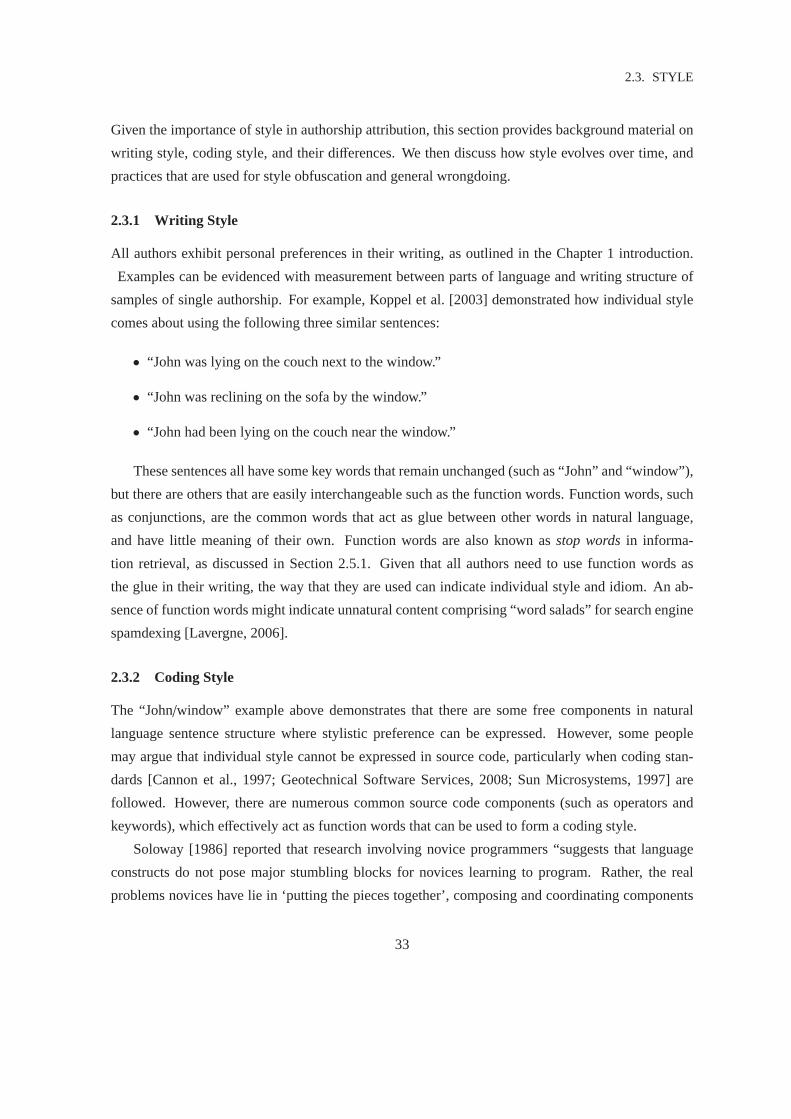
2.3. STYLE
Given the importance of style in authorship attribution, this section provides background material on
writing style, coding style, and their differences. We then discuss how style evolves over time, and
practices that are used for style obfuscation and general wrongdoing.
2.3.1 Writing Style
All authors exhibit personal preferences in their writing, as outlined in theChapter 1 introduction.
Examples can be evidenced with measurement between parts of language and writing structure of
samples of single authorship. For example, Koppel et al. [2003] demonstrated how individual style
comes about using the following three similar sentences:
• “John was lying on the couch next to the window.”
• “John was reclining on the sofa by the window.”
• “John had been lying on the couch near the window.”
These sentences all have some key words that remain unchanged (suchas “John” and “window”),
but there are others that are easily interchangeable such as the functionwords. Function words, such
as conjunctions, are the common words that act as glue between other words in natural language,
and have little meaning of their own. Function words are also known asstop wordsin informa-
tion retrieval, as discussed in Section 2.5.1. Given that all authors need to use function words as
the glue in their writing, the way that they are used can indicate individual styleand idiom. An ab-
sence of function words might indicate unnatural content comprising “word salads” for search engine
spamdexing [Lavergne, 2006].
2.3.2 Coding Style
The “John/window” example above demonstrates that there are some free components innatural
language sentence structure where stylistic preference can be expressed. However, some people
may argue that individual style cannot be expressed in source code, particularly when coding stan-
dards [Cannon et al., 1997; Geotechnical Software Services, 2008;Sun Microsystems, 1997] are
followed. However, there are numerous common source code components (such as operators and
keywords), which effectively act as function words that can be used to form a coding style.
Soloway [1986] reported that research involving novice programmers “suggests that language
constructs do not pose major stumbling blocks for novices learning to program. Rather, the real
problems novices have lie in ‘putting the pieces together’, composing and coordinating components
33

CHAPTER 2. BACKGROUND
of a program”. Therefore the way that even novice programmers use language constructs and put
them together demonstrates individual style.
The presence of coding standards also generates stylistic differences in itself, as there is a “lack
of consensus” between publications on programming style and standards [Oman and Cook, 1990],
and “no guidelines on how to resolve conflicts between rules” [Oman and Cook, 1988].
2.3.3 Similarities and Differences between Writing and Coding Style
Oman and Cook [1988] argued why writing style and programming style are similar. They explained
that “effective writing is more than observing established conventions for spelling, grammar and
sentence structure”, similar to how effective programming is more than just following style guides.
In writing there is “perception and judgement a writer exercises in selecting from equally correct
expressions, the one best suited to his material, audience, and intention” [Oman and Cook, 1988].
Similarly, a programmer must choose the appropriate operators, keywordsand library functions from
which many equally correct options could be chosen. Moreover, Oman and Cook [1988] explained
that some books on programming style have been derived from books on natural language style.
A key difference between writing and coding style is the lower amount of flexibility that can
be demonstrated when coding, as “computers are far less forgiving thanhumans of imprecision and
difference in usage” [Michaelson, 1996], and “in computers the compiler andrun-time system are the
ultimate arbiters of program acceptability” [Michaelson, 1996].
Another key difference is the disparity between the vocabulary size in natural language and the
number of constructs in code. For example, there are around one million English words today [Ling,
2001], which is far more than the number of features in the C programming language, with thirty-
two keywords, thirty-nine operators, and fifteen modest header files, containing the standard library
functions and constants [Kelly and Pohl, 1997]. The disparity may be further increased with the
introduction of words with spelling mistakes in natural language, since there isless scope for mistakes
in source code that must follow strict syntax rules for compilation.
2.3.4 Evolving Style
Since authorial writing style evolves over time, the earliest work samples become the least reliable
indicators of current writing style. For example, Can and Patton [2004] studied the changes in writ-
ing style of two Turkish authors spanning twenty-seven and fifty-six years respectively. With work
samples organised into “old” and “new” categories, they found a statisticallysignificant difference in
the average word length between these categories.
34

2.3. STYLE
In another study, Pennebaker and Stone [2003] found that as individuals age, they “use more
positive and fewer negative affect words, use fewer self-references, use more future-tense and fewer
past-tense verbs, and demonstrate a general pattern of increasing cognitive complexity”.
To the best of our knowledge, there is no previous research for empirical evaluation of evolving
programming style for programmers. Instead, Kemerer and Slaughter [1999] researched the evo-
lution in twenty-three software projects, spanning a twenty year period and25,000 change events.
However, this is not helpful for studying the evolution of programming style inindividuals. Kemerer
and Slaughter [1999] noted that “it is not surprising that empirical research on software evolution is
scarce. The researcher has to collect data at a minimum of two different points in time. This cre-
ates practical difficulties in terms of sustaining support for the project over this period and/or finding
an organisation that collects and retains either relevant software measurement data or the software
artefacts themselves”. Therefore, we expect that our work in Chapter6 is the first to empirically
evaluate the evolution of programming style in individuals, with our experiments that use a collection
of student programming assignments spanning six distinct points in time.
2.3.5 Dishonest Style
Kacmarcik and Gamon [2006] demonstrated that substituting just 14 words per 1,000 is sufficient
to reduce correct authorship attributions by 83%. The key is to “identify thefeatures that a typical
authorship attribution technique will use as markers and then adjust the frequencies of these terms
to render them less effective on the target document”. Kacmarcik and Gamon [2006] have also com-
mented that “idiosyncratic formatting, language usage and spelling” are tell-tale signs of authorship,
and that simple use of spelling and grammar checkers, for example, will return documents to “con-
ventional norms” making authorship attribution more difficult.
All of the above strategies can be used to mask authorship when dealing with law enforcement.
But there are also more legitimate reasons for anonymisation, such as organisational whistle-blowers
who feel the need to report bad behaviour and wish to avoid drawing attention to themselves [Kac-
marcik and Gamon, 2006].
Palkovskii [2009] wrote about counter plagiarism detection software that has been used to obfus-
cate assignments, so that plagiarism detection software is rendered useless. These algorithms involve
substituting characters from one natural language to another that appear identical to the human eye,
but are from different character sets and are hence treated differently in plagiarism detection software.
For example, the Greek letters ‘α’ (alpha) and ‘ν’ (nu) closely resemble English letters ‘a’ and ‘v’.
However, some differences cannot be discerned at all by the human eye. For example, Palkovskii
[2009] suggested the replacement of the English letter ‘o’ with a similar circular Russian charac-
35
CHAPTER 2. BACKGROUND
ter. Likewise, other substitutions involve replacing all spaces with a non-space character in a white
colour, so that it visually appears as a regular space. Methods to detectthe use of this kind of soft-
ware include transforming the content into ordinary ASCII text, so that obfuscations that are effective
in word processing software would be undone. Authorship attribution software needs to be robust
against the substitutions described above. The use of n-grams is a robust method we use in Chapter 5
as introduced in the next section.
2.4 Measuring Style
In this section we review the methods used to quantify coding style. We begin bydiscussing software
metrics, which is by far the most common approach. We then review n-grams, watermarking, and
existing automated tools. This section is concluded with a brief overview of other methods used for
measuring style in natural language.
2.4.1 Metrics in the Literature
Software metrics are important in measuring aspects of source code such as correctness, efficiency,
readability, understandability, modifiability, and verifiability [Harold, 1986].They are used in project
management for predicting development effort [Gray and MacDonell, 1997]. They are also valuable
in authorship attribution when measuring style.
A very comprehensive description of software metrics is the chapter by Conte et al. [1986,
chap. 2]. This chapter organises metrics in the literature under a taxonomy of eight headings: size
metrics, data structure metrics, logic structure metrics, composite metrics, software science compos-
ite metrics, effort and cost metrics, defect and reliability metrics, and design metrics, whichwe now
discuss in turn.
Size metricsare generally simple count-based metrics such as lines of code, token counts, and
function counts. Further examples are the well-known Halstead metrics [Halstead, 1972], including
number of unique operatorsn1, number of unique operandsn2, total occurrences of operatorsN1,
and total occurrences of operandsN2. Another well-known example is the COCOMO (COmparative
COst MOdel) metric [Kemerer, 1987], for estimating effort based on the proportion of new and reused
code in a project.
Data structure metricsrefer to how data is used. Examples include the amount of input and
output data processed by a program, live variables, variable spans, and data sharing between modules.
This category should not be confused with programmatic data structures, such as lists, trees, and
hashtables.
36
2.4. MEASURING STYLE
Logic structure metricsrelate to the use of branching and looping constructs such as decision
counts, minimum number of paths, component reachability, nesting levels, andunnatural program
flow such as the use of goto statements [Dijkstra, 1968]. This category alsoincludes Halstead’s
cyclomatic complexity measure [Halstead, 1972]. This metric measures the complexity of a program
represented as a graph, with decision statements represented as nodes and pathways represented by
edges.
We list the last five categories in the taxonomy very briefly:composite metricsrefer to metrics
consisting of multiple components;software science composite metricsrefer to new metrics devel-
oped from Halstead’s basicn1, n2, N1, andN2 measurements;effort and cost metricsrefer to mea-
sures concerning time and money;defect and reliability metricsrefer to measurements for creating
error-free and robust software; anddesign metricsrefer to high-level concepts such as coupling and
cohesion.
The above categories are very specific, and there are many general properties that the metrics
share. First, some of the above metrics are based on raw counts such as “number of functions” and
“number of decision statements”. These metrics are sensitive to the amount of code. That is, larger
source code samples will generally provide higher measurements for thesemetrics. Therefore it
becomes important to usenormalisedvariations in some applications such as authorship attribution.
Normalised metrics are important as they capture intrinsic properties of code such as function density,
rather than other properties such as source code length.
Other metrics can be measured on a continuous scale and can therefore be represented as his-
tograms with one bar for each measurement. For example, Lange and Mancoridis [2007] discussed
the line-lenexample, whereby the line lengths of source code samples are recorded with one bar for
every measurement from zero characters up to the longest line length. This technique can generate
very large numbers of measurements from just one metric such as theline-lenexample. This can be
managed by comparing entire histograms against one another using distance-based measures such as
the nearest neighbour measurement [Lange and Mancoridis, 2007]. Another technique to manage the
feature space is discretisation for grouping individual measurements, asdiscussed in Section 2.6.4.
An alternate implementation of software metrics is the use of linguistic labels instead of num-
bers. Gray and MacDonell [1997] referred to these as “fuzzy logic”metrics. Gray and MacDonell
[1997] suggested that fuzzy logic metrics provide “considerable benefits in terms of reducing com-
mitment, making full use of knowledge and improving interpretability”. For example, fuzzy logic
metrics could specify a “large number of screens” or a “low level of system complexity” [Gray and
MacDonell, 1997]. These examples require numeric measurements using hard boundaries between
classes, so describing these metrics as “fuzzy” may seem counter-intuitive. The use of linguistic
37

CHAPTER 2. BACKGROUND
labels is essentially a discretisation mechanism as described in Section 2.6.4. Other fuzzy metrics
are used to remark on how well comments match code, and how meaningful the identifiers are, for
example [Kilgour et al., 1997].
2.4.2 N-Grams
N-grams are sequences of adjacent tokens of lengthn. That is, a sequence oft tokens will generate
t−n+1 n-grams. N-grams are useful in capturing information about tokens thatoccur near one an-
other, which the stand-alone metrics discussed in Section 2.4.1 above cannot do. They are also robust
to changes in the content, as any content substitution will only affect a few overlapping n-grams. For
natural language, n-grams have been used for characters [Cavnarand Trenkle, 1994], words [Barron-
Cedeno et al., 2009], and parts of speech [Lioma, 2007] such as nouns, verbs, adjectives, adverbs,
conjunctions, and pronouns. For source code, they have been usedfor characters [Frantzeskou et al.,
2006a], bytes from executables [Maloof and Kolter, 2004], and tokens such as operators and key-
words [Burrows et al., 2006].
2.4.3 Watermarking
Watermarking refers to hiding authorship information within work. Source code watermarks, for
example, can be identifying patterns of space and tab characters [Daly and Horgan, 2005] at the end
of a file, which do not affect software execution. To successfully implement watermarking, trust
is needed in the party that resolves disputes, and there must be guarantees that dispute winners are
indeed rightful authors [Adelsbach and Reza Sadeghi, 2003]. Watermarking can potentially make
other means of measuring style redundant if successfully deployed, since the meaning of unmodified
watermarks should be absolute.
2.4.4 Automated Tools
Authorship attribution is very time-consuming to conduct manually, so any software tool that can aid
the process is highly valuable. For example, expert witnesses may be required to give evidence to
explain authorship traits, and computer software may be used to expedite the collection and summary
of evidence.
The Java Graphical Authorship Attribution Program (JGAAP) [Juola et al., 2006] is an example
of a natural language authorship attribution package, providing “textualanalysis, text categorisation,
and authorship attribution” functionality [Juola, 2010]. Other researchers have discussed the use of
natural language authorship attribution software at the prototype stage only [Cook, 2003; Kar, 2001].
38

2.5. INFORMATION RETRIEVAL FUNDAMENTALS
Such software does not yet exist for source code authorship attribution. The closest available
work is software that expedites the collection of software metrics, which canbe used as features
for making authorship decisions. Thepmccabesoftware does “McCabe-style function complexity
and line counting for C and C++” [Bame, 2010]. TheCCCCsoftware (C and C++ Code Counter)
“is a tool which analyses C++ and Java files and generates a report on various metrics of the code.
Metrics supported include lines of code, McCabe’s complexity and metrics proposed by Chidamber
& Kemerer and Henry & Kafura” [Littlefair, 2010]. TheEssential Metricssoftware “is a command
line metrics tool for C/C++ and Java software projects” [Power Software, 2010]. Counting metrics,
Halstead metrics, complexity metrics and object-oriented metrics are included. Thisis a commercial
product, but a trial version is available. Finally, theIDENTIFIED package [Gray et al., 1998] has
been used to compute twenty-six metrics by MacDonell et al. [1999] in their source code authorship
attribution work. The metrics in part relate to white space usage and normalisedcounts of individual
tokens.
2.4.5 Natural Language Measurements
Measuring style in natural language is beyond the scope of this thesis, so we just mention this area
briefly. Measurements for natural language include word length, sentence length, distribution of
syllables, parts of speech, function words, and word frequencies [Holmes, 1994]. Koppel et al. [2003]
showed that “frequent but unstable features are especially useful for style-based text categorisation”.
2.5 Information Retrieval Fundamentals
Manning et al. [2009] defined information retrieval as follows:
“Information retrieval (IR) is finding material (usually documents) of an unstructured na-
ture (usually text) that satisfies an information need from within large collections (usually
stored on computers).”
Since search engines are an important application of information retrieval, this section begins
with an overview of search engine architecture. We then follow with detail about the indexing and
querying components and models that are of most relevance to our work. This section concludes with
an overview of measures for evaluating the effectiveness of search engines.
39

CHAPTER 2. BACKGROUND
Users
Interface Query Index Indexer Crawler
Web
Engine
Centralised SearchEngine Architecture
Figure 2.5: A centralised search engine architecture comprising an interface, query engine, index,indexer module, and a crawler. This figure is modelled on a diagram by Baeza-Yates and Ribeiro-Neto [1999, p. 374].
2.5.1 Search Engines
Industry-scale search engines have numerous components that work together to facilitate indexing
and querying of content [Brin and Page, 1998]. The search engine requirements in this thesis are less
onerous, given that we are not using search engines to index billions ofdocuments, which requires
a distributed architecture for extreme scalability, and redundancy to mitigate failure. Instead, we use
a centralised architecture that is described by Baeza-Yates and Ribeiro-Neto [1999], as comprising
an interface to users, a query engine, an index, an index module, and a crawler to harvest content as
shown in Figure 2.5.
Thecrawler module is responsible for traversing and obtaining content from the Web for index-
ing. However, we mention this component for completeness only, since this is the only component
that we do not use in our work.
The indexermodule is responsible for extracting term and occurrence data from crawled pages.
Pre-processing often takes place before data is stored in theindex, such as stopping, stemming, and
case-folding [Witten et al., 1999, pp. 145–150].
40

2.5. INFORMATION RETRIEVAL FUNDAMENTALS
Stoppinginvolves omitting very common terms, which offer little value when retrieving docu-
ments. For example, Kelk [2010] listed the five most common UK English words as“the”, “and”,
“to”, “of”, and “a”, which are all good candidate stop words identified from a collection of twenty-
nine literary works. However, care needs to be taken that any stop list does not adversely impact
queries consisting of stop words. For example, the band name “The Who” and the Shakespearean
phrase “to be or not to be”, both consist of words that could all be potentially stopped.
Stemminginvolves transforming words to common base forms by eliminating prefixes and suf-
fixes, so that word variations can be equated. For example, the words “plays”, “played” and “playing”
can all be reduced to the root form “play”. However, care needs to betaken that word meaning is not
lost. For example, stemming “replay” to “play” is less appropriate in the above example. In addition,
“flies” and “flying” stem to a nonsensical word “fl”.
Case foldinginvolves transforming character case to a consistent case for ease of processing.
For example, capitalised words would be treated equivalently as those typedentirely in lower case.
Finally, other pre-processing is often necessary such as removing punctuation and correcting spelling
errors.
The indexmodule is for storing term and occurrence data for efficient lookup. The index is often
referred to as aninverted index, as the organisation of its data is in reverse to the norm. For example,
a standard book is organised by page number with headings, paragraphs, sentences, and words on
each page. Conversely, the inverted index is organised by term with occurrence data to follow, which
is more akin to an index of terms at the end of a text book. Index structures and components are
described in detail in Section 2.5.2.
The querymodule is responsible for receiving keywords provided by the user in theinterface
module, and retrieving document identifier and term occurrence data fromthe index. Keyword pre-
processing is again performed as necessary (stopping, stemming, and case-folding) to be consistent
with the pre-processing steps performed in index construction. After receiving candidate documents,
the query module (or a separate module) is then responsible for ranking thedocuments from most
relevant to least relevant [Arasu et al., 2001]. Ranking is performed using a similarity measure to
quantify document relevance. Several similarity measures are describedin detail in Section 2.5.3.
Finally, the ranked list of documents is returned to the interface module for viewing by the user.
Theinterfacemodule is responsible for generating web pages for the user. Initially, this will sim-
ply be a page with a text form field and a submit button for entering keyword searches. When a search
is submitted and a ranked list of results is returned, the interface module will then render the results as
a list with clickable items. Additional functionality will typically be present in industry-scale search
engines, such as the ability to automatically run related searches, view cached documents, and view
41

CHAPTER 2. BACKGROUND
similar pages.
2.5.2 Index Structures
Figure 2.6 shows an example of an inverted index created from the contentsof two documents. The
content of these documents simply comprises one sentence each from Section 2.5.1. Case-folding
has been applied to these documents, and punctuation has been removed. However, no stopping or
stemming has been applied in this example.
The inverted index contains two essential components: the lexicon and the inverted lists. The
lexiconcomprises a sorted list of all terms in the collection with one entry per term.
The inverted listscontain term occurrence data for each term in the lexicon including the collec-
tion frequency (ft), document identifier (d), and within-document frequency (fd,t). In a collection of
N documents, the inverted lists can be generically represented as:ft : [d1, fd1,t], [d2, fd2,t], ..., [dN, fdN,t].
The collection frequency (ft) tells us the number of documents that the term occurs in. The doc-
ument identifier (d ∈ d1, ...,dN) is a code to uniquely identify a documentDd. The within-document
frequency (fd,t ∈ fd1,t, ..., fdN,t) tells us the number of times termt appears in documentDd.
Other data can be included in the inverted lists. For example, pre-computed values for com-
ponents of some similarity measures described in Section 2.5.3 can be stored, which only require
computation once per document. The inverted lists can also include term offset information in the
documents, which is useful in identifying adjacent terms inphrase queries[Bahle et al., 2002]. For
example, the inverted list for the term “for” with offsets is “2 : [1,1, 〈5〉], [2,2, 〈4,10〉]”, with the first
term in each document being assigned a zero offset.
Inverted lists are usually also highly compressible. For example, an invertedlist for a common
stopword in a large document collection would be very long. Therefore, document identifiers and
offsets can be stored as small gaps relative to one another instead of large whole numbers. Higher
compression is achieved with this approach, as the number of distinct integers is reduced. This tech-
nique is known asd-gapsin the literature [Anh and Moffat, 2005], but we do not discuss compression
further as it is beyond the scope of this work.
2.5.3 Models for Query Matching
Models for query evaluation aim to assign a similarity score between queries and documents, with the
documents having the highest similarity scores being deemed the most relevant.Similarity measures
implement some or all of the following core ideas: term frequency, inverse document frequency, and
inverse document length, which we now discuss.
42

2.5. INFORMATION RETRIEVAL FUNDAMENTALS
the indexmoduleis forstoringterm andoccurrencedata foreff icientlookup
the indexermodule isresponsiblefor extract ingterm andoccurrencedata fromcrawledpages
(2)
(1) Lexicon Inverted Lists
Documents Inverted Index
and
crawled
data
eff icient
extract ing
for
f rom
index
indexer
is
lookup
module
occurrence
pages
responsible
storing
the
term
2: [1,1], [2,1]
1: [1,1]
2: [1,1], [2,1]
1: [2,1]
1: [1,1]
2: [1,1], [2,2]
1: [1,1]
1: [2,1]
1: [1,1]
2: [1,1], [2,1]
1: [2,1]
2: [1,1], [2,1]
2: [1,1], [2,1]
1: [1,1]
1: [1,1]
1: [2,1]
2: [1,1], [2,1]
2: [1,2], [2,1]
Figure 2.6: An inverted index showing the lexicon and inverted lists created from the content of twoexample documents in the left of the figure.
43
CHAPTER 2. BACKGROUND
When evaluating the similarity of a query to a pool of documents, some documentswill have
more instances of the query term(s) than others. Therefore documents witha higherterm frequency
should be weighted higher.
In addition, since documents will usually have a mixture of common and rare terms, it is ex-
pected that rarer terms that appear in fewer documents are more suitable for distinguishing relevance.
Therefore documents with a higherinverse document frequencyshould be weighted higher.
Moreover, it is expected that documents will be of unequal length, and longer documents should
not be considered more relevant simply due to having more words that can potentially match query
terms. Therefore documents with a higherinverse document lengthshould be weighted higher.
This thesis in part explores the Cosine [Witten et al., 1999, pp. 185–188],Okapi BM25 [Sparck-
Jones et al., 2000a;b], language modelling with Dirichlet Smoothing [Zhai andLafferty, 2004], and
Pivoted Cosine [Singhal et al., 1996] measures, which implement the aboveideas to varying extents.
Therefore we review the above similarity measures now. These are chosen because they are imple-
mented in the Zettair search engine [Search Engine Group, 2009], which forms part of the experi-
mental setup used in this thesis. A more complete review of information retrieval similarity measures
can be found in the book by Baeza-Yates and Ribeiro-Neto [1999]. Forreference, common symbols
in information retrieval are summarised below [Zobel and Moffat, 1998].
t: A term.
q: A query identifier.
Q: A query.
|Q|: Query length (number of terms in queryQ).
d: A document identifier.
Dd: A document with identifierd.
|Dd|: Document length (number of terms in documentDd).
N: Number of documents in the collection.
fq,t: Within-query frequency (number of occurrences of termt in queryq).
fd,t: Within-document frequency (number of occurrences of termt in documentd).
ft: Raw document frequency (number of documents in which termt appears).
44

2.5. INFORMATION RETRIEVAL FUNDAMENTALS
Ft: Collection frequency (number of occurrences of termt in the collection).
F: Total number of terms in the collection.
These terms form part of the information retrieval glossary in Appendix A.2.
Cosine
The Cosinesimilarity metric is based on the vector space model in which queries and documents
are plotted in multi-dimensional space with one dimension per term. Similarity is computedusing
the angle between the vectors. The query and document pair that has the smallest angle will give
the largest Cosine value. The largest possible Cosine value is obtained when there is zero degrees
between vectors [Witten et al., 1999, p. 186]. Witten et al. [1999] definedthe Cosine measure as:
Cosine(Q,Dd) =1
WqWd×
∑
t∈Q∩Dd
wq,t ×wd,t, where (2.2)
Wq =
√
√
n∑
t=1
w2q,t, Wd =
√
√
n∑
t=1
w2d,t, wq,t = ln
(
1+Nft
)
, wd,t = 1+ ln fd,t, and
• Wq is the Euclidean length (or weight) of the query,
• Wd is the Euclidean length (or weight) of documentd,
• wq,t is the query-term weight, and
• wd,t is the document-term weight.
In this formula,WqWd implements inverse document length,wq,t implements inverse document
frequency, andwd,t implements term frequency.
Okapi BM25
The Okapi BM25metric is based on the probabilistic model. Sparck-Jones et al. [2000a] gave a
simplified account of the development of the probabilistic model from the probabilistic theory. They
define the probability of relevance as:
“What is the probability that this document is relevant to this query?” [Sparck-Jones
et al., 2000a]
45

CHAPTER 2. BACKGROUND
Sparck-Jones et al. [2000a] then introduced the following two events based upon documentDd
and queryQ as a starting point to guiding the reader through the theory and mathematics:
1. “L, thatDd is liked, i.e. is relevant toQ”, and
2. “L̄, thatDd is not liked, i.e. is not relevant toQ”.
With these definitions, it would then be useful to calculate the probability that a document de-
scription Dd is liked L for judging relevance. Therefore, the remainder of the Sparck-Jones et al.
[2000a] overview discusses how to calculateP(L|D), and then introduces probabilistic theory for
individual terms. The final model is defined as:
OkapiBM25(Q,Dd) =∑
t∈Q
wt ×(k1+1) fd,t
K + fd,t×
(k3+1) fq,tk3+ fq,t
, where (2.3)
wt = ln
(
N− ft +0.5ft +0.5
)
, K = k1×
(
(1−b)+b× |Dd|
|Davg|
)
, and
• |Davg| is the average document length, and
• b, k1 andk3 are free parameters.
In this formula,wt implements inverse document frequency,(k1+1) fd,tK+ fd,t
implements term frequency,
andK implements inverse document length.
Parametersb, k1 andk3 are used to modify the effect of inverse document length, document-
term frequency, and query-term frequency respectively. Parameters b andk1 are commonly assigned
valuesb= 0.75 andk1 = 1.2 [Robertson and Walker, 1999]. Parameterk3 is assignedk3 = 0 for short
queries such as web queries, otherwise a large number is used such ask3 = 7 or k3 = 1,000, which is
“effectively infinite” [Robertson and Walker, 1999].
Okapi BM25 [Robertson and Walker, 1999; Sparck-Jones et al., 2000a;b] has been developed in
the Text REtrieval Conference (TREC) competitions [National Institute of Standards and Technology,
2010] with known relevance judgements. The formula given above is the one to be used in the absence
of relevance judgements [Sparck-Jones et al., 2000a;b].
Language Modelling with Dirichlet Smoothing
Dirichlet smoothing is a method to smooth a language model. The idea of language modelling ap-
proaches “is to estimate a language model for each document, and to then rank documents by the
likelihood of the query according to the estimated language model” [Zhai and Lafferty, 2004]. Based
46

2.5. INFORMATION RETRIEVAL FUNDAMENTALS
upon the earlier work by Ponte and Croft [1998] and Zhai and Lafferty [2004], we provide the defini-
tion that best uses our notation from Appendix A.2 by Bernstein et al. [2005] whom define the model
as:
log(P(Q|Dd)) = |Q| × ln
(
µ
µ+ |Dd|
)
+∑
t∈Q∩Dd
ln
(
F × fd,tµ×Ft
+1
)
, where (2.4)
• µ is the smoothing parameter.
The smoothing parameter is used to provide a mechanism to compensate for words that do not
appear in documents [Zhai and Lafferty, 2004]. This can occur regularly for short documents in
particular. Therefore, the smoothing parameter creates a balance between the language model of the
document and the language model of the whole collection. The Dirichlet smoothing parameter isµ,
which has been shown to produce effective results when set to 1,500 [Bernstein et al., 2005].
Pivoted Cosine
Singhal et al. [1996] noted that “better retrieval effectiveness results when a normalisation strategy
retrieves documents with chances similar to their probability of relevance”. The balance between
probability of relevance and probability of retrieval can be upset in the Cosine measure, for exam-
ple, due to “the long held belief that Cosine normalisation tends to favour short documents in re-
trieval” [Singhal et al., 1996]. Therefore, apivot is a applied to correct the imbalance on the existing
normalisation scheme, by tilting the normalisation scheme at the pivot point so thatthe scheme is
boosted on one side of the pivot, and reduced on the other. For example,the normalisation scheme in
the Cosine measure iswq,t ×wd,t, therefore the pivoted normalisation for Cosine can become:
PivotedNormalisation= (1− slope)× pivot+ slope× (wq,t ×wd,t). (2.5)
The slopeis the gradient of the line that passes through the pivot point [Singhal etal., 1996].
The implementation in the Zettair search engine [Search Engine Group, 2009]suggests using a pivot
of 0.2.
2.5.4 Effectiveness Quantification
Having covered indexing, querying, and search engines in general, itis now necessary to discuss how
to measure search engine effectiveness. Effectiveness is measured by the quality of search engine
results as judged by users or determined by relevance judgements. Numerous measurements are
47

CHAPTER 2. BACKGROUND
Y ZX
Retrieved Relevant
W
Figure 2.7: Visual representation of definitions for precision and recall [Moffat and Zobel, 2008].X is the set of relevant documents that have been retrieved (true positives), Y is the set of retrieveddocuments that were not relevant (false positives), Z is the set of relevant documents that were notretrieved (false negatives), and W is the set of documents that were neither retrieved or deemedrelevant (true negatives). According to this diagram, precision is|X|
|X|+|Y| and recall is |X||X|+|Z| .
available for quantifying effectiveness, and this thesis covers precision, recall, reciprocal rank, and
average precision. Other measures such as normalised discounted cumulative gain [Jarvelin and
Kekalainen, 2002], and rank-biased precision [Moffat and Zobel, 2008], are not covered.
Precision and Recall
Precision and recall are simple and commonly used evaluation metrics. Numerous definitions are
available, but perhaps one of the best explained is the Venn-diagram representation by Moffat and
Zobel [2008] reproduced in Figure 2.7.
Figure 2.7 represents a pool of documents, some of which are retrieved by an information retrieval
system (RegionY), and others that are judged relevant (RegionZ). In the perfect scenario, these
two sets will overlap exactly, but this is difficult to achieve. Precision is defined as the proportion
of retrieved documents that are relevant(
|X||X|+|Y|
)
, and recall is defined as the proportion of relevant
documents that are retrieved(
|X||X|+|Z|
)
. RegionW represents irrelevant documents that have not been
retrieved, which does not take part in precision or recall calculations.
A variation of precision is P@X or precision at cutoff X, whereX is a fixed number of retrieved
48
2.6. MACHINE LEARNING FUNDAMENTALS
documents. Common uses are P@10 for evaluating the relevance of the firstpage of results returned
by current, popular Internet search engines, and P@1 for evaluatingjust the correctness of the top
result.
Finally, the F-measure [Rennie, 2004] (orF1 score) is used to generate a value that represents a
compromise between precision and recall:
F1 =2× precision× recall
precision+ recall(2.6)
Reciprocal Rank and Mean Reciprocal Rank
Reciprocal rank measures the reciprocal value of the position of the first relevant (or correct) result
from a ranked list. So if the first correct result was position 3, then the reciprocal rank would be13.
Then, Mean Reciprocal Rank (MRR) is used to average multiple reciprocal rank scores to measure
overall system performance.
Average Precision and Mean Average Precision
Average precision measures the precision of every relevant (or correct) result from a ranked list and
takes the average. For example, if correct results are at positions 2, 3,and 9 in a ranked list of ten
documents, then average precision is(
12 +
23 +
39
)
/3 = 12. Similar to MRR, Mean Average Precision
(MAP) is used to average multiple average precision scores to measure overall system performance.
2.6 Machine Learning Fundamentals
Cunningham et al. [1997] described a purpose of machine learning as “to devise algorithms that can
supplement, or supplant, domain experts in knowledge engineering situations”. Cunningham et al.
[1997] also mentioned a key link between information retrieval and machine learning that forms a
significant component of this thesis:
“Using learning algorithms to automate information retrieval processes such as docu-
ment classification ... can alleviate the workload of information workers and reduce in-
consistency introduced by human error.”
This section provides an overview of machine learning to ensure that enough is understood for
classification in authorship attribution. We begin by describing the training andtesting phases for a
typical classification problem. Then we cover cross-validation, feature selection, and discretisation
49

CHAPTER 2. BACKGROUND
topics that specifically arise in this thesis. Numerous text books are availablesuch as the data mining
book by Witten and Frank [2005] for further reading on machine learning.
2.6.1 Training and Testing
This thesis introduces information retrieval ranking for source code authorship attribution in Chap-
ter 5. However, most of the prior source code authorship attribution work(covered in Chapter 4), has
used machine learning classification algorithms to learn how to attribute authorship. Therefore, we
begin by discussing how machine learning algorithms can be used to attribute authorship.
A training phase is needed so that a classification algorithm canlearn how to classify existing
work samples of established authorship. Therefore, when a new sample ispresented, the classification
algorithm can assign authorship to the most likely author based on the learnedtraits. In experimenta-
tion, this step is a separatetestingphase, where the effectiveness of multiple classification algorithms
are often compared to one another, in order to identify the most suitable algorithm for the problem at
hand.
For authorship attribution with machine learning methods, accuracy is definedas the proportion
of times the classification algorithm assigns the testing samples to the correct author. The specific
classification algorithms that appear in this thesis are covered in Section 2.7.
2.6.2 Cross Validation
When classification experiments are organised into training and testing phases, a separate data set
is needed for each component. If accuracy scores were only reported for the trained data, the re-
sults would then beoverfittedto that data, and not representative of results obtained for new unseen
problems.
The simplest way to organise an experiment into training and testing phases is todivide the data
in half, and use one part for training and the other for testing. However,this approach is problematic
for small data sets in particular, as the amount of test data is reduced by half.
A solution is to repeat the above experiment a second time with the roles of the data reversed.
That is, use the testing half for training and the training half for testing for a secondfold, and then
combine the results with the first fold. This approach allows every sample to beused for testing in
turn, which increases the size of the result set. This experiment design is known as two-foldcross
validation[Witten and Frank, 2005, pp. 125–127].
Another problem still persists when using two-fold cross validation. That is, half of the data is
unavailable for training. This is particularly problematic when conducting source code authorship
50

2.6. MACHINE LEARNING FUNDAMENTALS
Fold Instances1 A1 B1 C1 D1 E12 A2 B2 C2 D2 E23 A3 B3 C3 D3 E34 A4 B4 C4 D4 E45 A5 B5 C5 D5 E56 A6 B6 C6 D6 E6
Figure 2.8: Thirty instances and five classes (A-E) spread across six folds. All folds have a documentfrom each class, therefore and all classes are perfectly stratified.
attribution experiments on student programming assignments, for example, as their coding styles
may be still evolving, and only some training samples may be truly helpful when attributing each
sample. It may be particularly difficult if the best samples are in the testing set when each sample in
the training set is classified in turn.
To overcome this second problem, the size of the training fold needs to be increased such that
more samples are available when constructing a model for classification. Thiscan be done by simply
increasing the two-fold experiment design to a larger number of folds, such as ten-fold. In ten-fold
cross validation, nine of the folds are used for training, and the remaining fold is used for testing.
This is then repeated nine more times, where the remaining folds are treated as the test fold in turn.
The size of the training set is therefore increased from 50% to 90% of the samples in the collection.
Another problem concerns collection properties such as the number of samples per author. For
example, consider a scenario with thirty samples in a collection, where the samples belong to five
authors with six samples per author each. Figures 2.8 and 2.9 depict what the folds could look like
when this collection is organised into six folds and ten folds respectively. There is a problem here, in
that when one fold is separated for testing, there is a527 chance to identify the author using a six-fold
experiment design (Figure 2.8), and a525 chance to identify the author using a ten-fold experiment
design (Figure 2.9), when working by random chance.
To alleviate this third problem, another cross-validation design is available called leave-one-out
cross validation [Witten and Frank, 2005, pp. 127–128]. In this variant,the number of folds is
maximised and set to the number of samples in the collection. This variation causesan efficiency
trade-off, as it can be slower to execute since the number of folds has been maximised.However,
this experiment design maximises the amount of training data, and is more suited to dealing with
collections with a varying number of samples per author, since problems demonstrated in Figures 2.8
and 2.9 cannot occur. The leave-one-out cross validation experimentdesign is used throughout this
thesis.
51

CHAPTER 2. BACKGROUND
Fold Instances1 A1 B5 D32 A2 B6 D43 A3 C1 D54 A4 C2 D65 A5 C3 E16 A6 C4 E27 B1 C5 E38 B2 C6 E49 B3 D1 E5
10 B4 D2 E6
Figure 2.9: Thirty instances and five classes (A-E) spread across ten folds. Each fold is only repre-sented by three of the five classes.
2.6.3 Feature Selection
The purpose of feature selection is to “identify and remove as much irrelevant and redundant informa-
tion as possible prior to learning”, which can generate “enhanced performance, a reduced hypothesis
search space, and, in some cases, reduced storage requirement” [Hall and Smith, 1998]. This is con-
tradictory to the idea of monotonicity that asserts that “increasing the number of features can never
decrease performance” [Hall and Smith, 1998]. However, this often does not apply to machine learn-
ing, since “adding irrelevant or distracting attributes to a dataset often ‘confuses’ machine learning
systems” [Witten and Frank, 2005, pp. 232].
Feature selection algorithms involve processes such as adding or removingone feature at a time
to a model until no further change improves classification accuracy. Alternatively, the value of indi-
vidual features can be evaluated one at a time for possible inclusion in a model.However, we do not
go into this further, as this thesis mostly uses existing feature set classes instead of exploring the use
of feature selection algorithms in detail.
2.6.4 Discretisation
Machine learning algorithms often need to process features with discrete orcontinuous values. Dis-
crete features are categorical. For example, gender as a feature has two categorical values: “male”
and “female”. Conversely, features that require measurement are often continuous such as height.
Continuous features can prove difficult for machine learning algorithms to process, and a solution
is to organise the possible values into a number of fixed ranges. This process is called bucketing,
binning, ordiscretisation[Shevertalov et al., 2009]. For example, when using height as a featurefor
52

2.7. CLASSIFICATION ALGORITHMS
human adults, the bins could be 140-149cm, 150-159cm, 160-169cm, 170-179cm, 180-189cm, 190-
199cm, and so on.
Several methods are available to determine bin boundaries such as therange, frequency, andge-
netic algorithmmethods [Shevertalov et al., 2007]. Range-based discretisation uses fixed boundaries
for the set of possible values such as the height example above. Frequency-based binning uses incon-
sistent ranges to keep the number of items in each bin roughly consistent. Genetic algorithm binning
uses machine learning techniques to determine effective bin combinations. We use range-based dis-
cretisation in Chapter 4 when reimplementing some of the previous work.
2.7 Classification Algorithms
This section presents an overview of the machine learning algorithms that have appeared in previ-
ous source code authorship attribution studies with empirical evaluations. The classifiers covered
are decision trees, nearest neighbour methods, neural networks, case-based reasoning, discriminant
analysis, regression analysis, support vector machines, voting feature intervals, Bayesian networks,
and simplified profile intersection. We do not attempt to cover all classification algorithms exhaus-
tively as there are simply far too many. For example, version 3.5.8 of the Wekamachine learning
toolkit [Holmes et al., 1994; Witten and Frank, 2005] that we use in our experiments has 114 classi-
fication algorithms available. Chapter 4 describes how the classifiers are used in the previous source
code authorship attribution work.
2.7.1 Decision Trees
A decision tree classifier is a tree structure with tests on the internal nodes and classes on the leaf
nodes. A document is classified by executing the tests and following the branches from the root level
until a leaf-level node is reached. Care must be taken that the tree does not become too large, as
lengthy branches may be too specific to be of general use to new unseen cases for classification [Se-
bastiani, 2002]. Numerous learning algorithms are available for decision trees, and this thesis uses
the C4.5 decision tree [Sebastiani, 2002], which has appeared in one previous source code authorship
attribution study [Elenbogen and Seliya, 2008].
2.7.2 Nearest Neighbour Methods
Nearest neighbour methods classify work based on patterns of the nearest sample using a distance
measure in vector space, for example. Storing all available samples can be prohibitive for large
53

CHAPTER 2. BACKGROUND
problems, so improvements to the basic algorithm attempt to reduce the number of stored comparison
samples [Kukolich and Lippmann, 2004].
A variation of the nearest neighbour algorithm is the K-Nearest Neighbour classifier (KNN).
This algorithm considers multiple nearest samples (K samples) instead of just one identified using
the Euclidean distance, and then voting is used to classify the testing sample based on the most
represented class in the set of nearest neighbours analysed [Kukolich and Lippmann, 2004].
2.7.3 Neural Networks
Neural networks are akin to “biological nervous systems” [Kukolich andLippmann, 2004]. Like
the human brain, a neural network is based upon a series of interconnected units where signals can
pass from unit to unit [Gray and MacDonell, 1999]. When implemented as a document classification
algorithm, there are inputs that are the features such as term frequenciesor higher level language
statistics, there are outputs that are the classes of interest (such as candidate authors), and there are
“dependence relations” that are weights for the connections in between [Sebastiani, 2002]. That is,
the term weight data is first populated in the input units, the data flows throughdependence relations
in the network, and the output unit(s) make the authorship decision [Sebastiani, 2002].
2.7.4 Case-Based Reasoning
Case-based reasoning (also known as analogy) involves using “specific knowledge of previously ex-
perienced, concrete problem situations” for solving new similar problems [Aamodt and Plaza, 1994].
A key difference to other machine learning algorithms is that case-based reasoning models are often
developed incrementally, as new cases are tested and added to the pool ofprevious cases [Aamodt
and Plaza, 1994]. This machine learning method also does not require an explicit model, since the
key idea is to determine meaningful features for representing cases [Watson, 1995]. For authorship
attribution, a “case” is an author. Authorship of new unseen samples can be assigned to the “case”
with the most features in common or nearest features.
2.7.5 Discriminant Analysis
Lachenbruch and Goldstein [1979] defined discriminant analysis as assigning “an unknown subject
to one of two or more groups on the basis of a multivariate observation”. In authorship attribution,
the multivariate observation can be a collection of measurements taken from software metrics. When
dealing with more than two candidate authors, the problem is referred to asmultiple discriminant
analysis [MacDonell et al., 1999]. Another variation iscanonicaldiscriminant analysis as used in
54
2.7. CLASSIFICATION ALGORITHMS
previous feature selection research [Ding and Samadzadeh, 2004], where features were reviewed one
at a time for inclusion in a final model, until the addition of further features no longer increased the
effectiveness of the model significantly. Terminating the inclusion of features inthis manner prevents
the model from becoming bloated, which is the fundamental idea ofcanonicaldiscriminant analysis.
Related to discriminant analysis isprincipal component analysis. Principal component analysis
is a method for obtaining meaningful facts from difficult or bloated data [Shlens, 2005]. That is, it
allows high dimensional data to be reduced to fewer and simpler dimensions. This method is again
particularly useful for identifying critical features for authorship attribution tasks.
2.7.6 Regression Analysis
Multiple regression analysis is based on prediction output variables from aseries of input vari-
ables [Stamatatos et al., 2000]. For authorship attribution, we just need the author as the dependent
variable, so (single) regression analysis is applicable here. The ability to examine the model is an
advantage of regression analysis. This could therefore be considered a white-box technique, which
also provides a mechanism to allow the modeller to verify the model [Stamatatos et al., 2000].
2.7.7 Support Vector Machines
Support vector machines can be used to separate work samples using a hyperplane in n-dimensional
space [Diederich et al., 2003]. A margin is used to separate positive and negative samples with the
maximum possible gap. New work samples are confirmed as belonging to an author if they fit on
the correct side of the hyperplane. Diederich et al. [2003] cited scalability as a major advantage for
support vector machines, as they are able to “process many thousand different inputs”.
2.7.8 Voting Feature Intervals
The voting feature interval classification algorithm represents each training sample as a vector with
measurements for each feature and a class label. Then all values for each feature in the training set
are bucketed into fixed intervals. When a new unseen example comes along inthe testing phase,
the candidate classes receive votes each time their feature interval matchesthat of the unseen ex-
ample. Then the class with the most votes is deemed the correct class. See the work by Demiroz
and Guvenir [1997] for more information on the algorithm. This is somewhat similar to coordinate
matching [Uitdenbogerd and Zobel, 2002], with the additional step of organising the feature space
into intervals.
55

CHAPTER 2. BACKGROUND
2.7.9 Bayesian Networks
Bayesian probability is based on the “degree of belief” of an event, rather than statistical deduc-
tion [Heckerman, 1996]. For example, the outcome of a coin flip can be determined statistically,
but the degree of belief in a tennis player winning a major tennis tournament is much harder to
evaluate. Bayesian probability is of use when modelling multiple variables, suchas trying to fig-
ure out the probability a tennis player has of winning a grand slam in any given calendar year. The
Bayesian network can handle this as it can represent a “joint probability distribution” from the vari-
ables involved [Heckerman, 1996]. This classifier has numerous benefits such as the ability to handle
incomplete data [Heckerman, 1996], but it is not one of the most scalable since the “asymptotic cost
is exponential” [Zhao et al., 2006].
2.7.10 Simplified Profile Intersection
The Simplified Profile Intersection (SPI) classification algorithm [Frantzeskou et al., 2005], is also
known as co-ordinate matching in information retrieval literature [Uitdenbogerd and Zobel, 2002].
This measure simply counts the number of features that are common between thetesting sample
and the combined samples of each candidate author. To keep the comparisons fair, the samples are
truncated at a fixed profile lengthL of theL most common features. A disadvantage of this approach
is that theL parameter is collection-sensitive.
To increase the feature space, this method can be applied on n-grams of features, which results
in the number of features in the feature space being increased to the powerof n. This method was
motivated by earlier work on a relative distance metric that included frequency information of the
n-grams [Keselj et al., 2003], however Frantzeskou et al. [2006a] showed that relative distance was
less accurate, particularly for low values ofn.
2.8 Summary
In this chapter, we reviewed the background literature necessary for understanding our contributions
in the remainder of this thesis in Chapters 3 to 7. We have reviewed the definitions of authorship
attribution and related areas, motivated the need for authorship attribution, discussed the differences
in writing and coding style, reviewed methods for measuring style, and covered necessary background
material in information retrieval, machine learning, and classification algorithms.Next, in Chapter 3
we present the comprehensive set of collections used for evaluating allempirical contributions in this
thesis.
56
Chapter 3
Collections
The first step in any authorship attribution study is the gathering of examples and possible collection
construction. Since we are not dealing with the author discrimination problem, the samples obtained
for constructing our collections must foremost be single-author. Moreover, the samples should ideally
be obtained from a source where they are organised by author, insteadof title or year, so that all
samples by any author can be obtained without risk of omitting some.
Obtaining samples for constructing source code collections is more challenging than for natural
language collections, since there are fewer sources of significant single-author samples. For example,
Stamatatos [2008] summarised many significant natural language collections such as the Reuters
collection, TREC collections, and other collections, which were built from newspaper articles, email,
forum messages, and blogs. Moreover, any online service with an author index is helpful for building
new natural language collections, such as browsing e-book authors atProject Gutenberg [Hart, 2010],
or bibliographic services such as the Digital Bibliography and Library Project (DBLP) [Ley, 2010].
Concerning source code samples, the bulk of the previously used collections are academic sam-
ples based on student programming assignments, which cannot be sharedfor intellectual property
reasons. Moreover, large software efforts tend to be collaborative in nature, which limits the avail-
ability of meaningful single-author samples. The collaborative software projects hosted on Source-
Forge [Geeknet Inc., 2010] is a good example of this. Initiatives for structured text such as the
Initiative for Evaluation of XML Retrieval (INEX) [Geva et al., 2009] forXML data exist, but there
is no equivalent for source code.
Given the limitations of existing source code collections, and limited sources to generate new
source code collections, this chapter introduces four new and significant collections for source code
authorship attribution, which are the largest used to date. We make the data asaccessible as we can
by releasing the data that is not covered by copyright or intellectual property concerns. Moreover, we
57

CHAPTER 3. COLLECTIONS
provide detailed statistics concerning the properties of the collections, and we document procedures
for the reproduction of our collections where applicable.
We begin this chapter in Section 3.1 by reviewing good practice of collection construction. We
introduce our four new collections in turn in Section 3.2, showing consideration to the good practice
topics. Next, we provide a summary of all key collection properties of our collections in Section 3.3,
which allows effective evaluation of results between collections in Chapters 4 to 7. The comparison of
our new collections to those used by other researchers follows in Section 3.4, where we demonstrate
the need and value of the collections we have put together. We explain the different purposes of our
collections in Section 3.5, and details concerning collection sharing and recreation in Section 3.6.
We conclude this chapter in Section 3.7, with a summary of the work covered and an introduction to
Chapter 4, where the first experiments that use our new collections appear.
3.1 Important Criteria for Collection Construction
Researchers constructing collections for authorship attribution should consider the following desir-
able properties: number of authors, number of samples per author, samplelengths, chunking avoid-
ance, representativeness, multiple author types, multiple languages, singleauthorship, correct author-
ship, no identifying features, and availability. We now explain each of thesein turn.
Having a highernumber of authorsin an authorship attribution experiment makes the problem
harder. For example, there is a 10% chance to identify the author by random chance in a ten-class
experiment, but the chance is reduced to 1% in a 100-class experiment, hence the naive baseline of
these two experiments differs by 9%. However, having more authors provides more flexibility in
experiment design. For example, having a large number of authors does not imply that all have to be
used at once, which means that random sampling could take place to allow additional runs. This can
in turn lead to more statistically significant outcomes.
Using moresamples per authoris almost always desirable, as this increases the amount of train-
ing data available to model author style. In addition, it is desirable to keep the number of training
samples per author consistent if possible, to eliminate bias towards the most prolific authors. How-
ever, any method to exclude training samples must be carefully considered.For example, simply
removing samples at random could result in some of the best training samples becoming unavailable.
Similar to having more samples per author, having longersample lengthsis also advantageous, as
this property again increases the amount of training data available. Keepingconsistent sample lengths
can reduce bias towards prolific authors, but it is not obvious where samples should be truncated if
this is to take place. Keeping sample lengths consistent may require unusual collection design.
58
3.1. IMPORTANT CRITERIA FOR COLLECTION CONSTRUCTION
Chunkingrefers to breaking complete samples into smaller parts, whether they are fixed-length
at the character or line level, or variable-length at the function or sourcefile level. Chunking in-
troduces a trade-off in that it can increase the number of samples per author whilst reducing the
sample lengths. Both previous empirical contributions in source code authorship attribution with
chunking have shown that authorship attribution accuracy is reduced when chunking is used [Ding
and Samadzadeh, 2004; Kothari et al., 2007]. This is not surprising, since single-author software
projects, such as student programming assignments, are often modest in length, hence reducing the
sample lengths of these samples may adversely affect the amount of training data. This thesis does
not require the use of chunking, since we use a large numbers of samplesper author. However, we
do not dismiss chunking universally, as it has been shown to be effective in other applications such as
passage retrieval [Kaszkiel and Zobel, 1997].
Representativeness[Biber, 1993] is key to maintaining sampling consistency across demographic,
social, and other factors. For example, the student authors identified when building a collection with
a large number of samples per author may not be representative of a typical student author, as the
prolific authors identified are more likely to be students who have done more than one degree, or have
repeated courses. However, representativeness may be unachievable if identifying or demographic
data is not available.
Collections should ideally representmultiple author typessuch as student, freelancer, and pro-
fessional author types. Some researchers have built collections comprising samples from authors
of varying backgrounds combined together [Ding and Samadzadeh, 2004; Krsul and Spafford, 1997;
MacDonell et al., 1999], which may have been necessary in some experiments where data was scarce.
However, we suggest it is preferable to use separate collections for work obtained from multiple au-
thor types, so that varying programmer experience within any individual collection can be removed
as a confound. For example, we would expect student-based collectionsto be more difficult to clas-
sify given the lower skill level and developing programming styles of these individuals. We show
supporting evidence of this in Chapter 6.
Testingmultiple languagesis also important as the features available in each language will de-
termine the authorship markers that can be used. Programming languages that are more feature-rich
will increase the number of authorship markers available, and hence increase the difficulty of an
experiment. Feature-rich languages are those with more language features such as keywords and
operators.
Samples must be ofsingle authorshipfor authorship attribution. Collections with samples of mul-
tiple authorship are only of value in authorship discrimination problems as discussed in Section 2.1.2.
This property can be difficult to satisfy as many software projects are collaborative in nature.
59

CHAPTER 3. COLLECTIONS
Samples must also be ofcorrect authorshipwithout copied, reused, reproduced, or plagiarised
content. This property is sometimes difficult to meet in cases where citation and quotation practices
are poor, such as in student assignment work. Moreover, any sample that has legitimately reused
content should be questioned as to whether the sample should be used at all,since the reused content
is only representative of the cited author. For example, Clough et al. [2002] discussed the METER
collection with legitimate journalistic text reuse, which would be unsatisfactory for an authorship
attribution experiment. Clough and Stevenson [2009] have also created a collection with simulated
plagiarism fragments inserted, but simulating legitimate writing may not be possible.
Collection data must also have noidentifying featuressuch as name, contact details, or affiliations.
Effort is needed to omit these details so that authorship attribution experiments canrely on writing
style alone as intended.
Finally, collectionavailability is also important so that other researchers can reproduce the work
and avoid duplication of effort. This property is challenging to achieve, as copyright and intellectual
property must be considered, permissions must be sought, and some data simply cannot be released
at all due to privacy reasons.
The properties discussed above were identified in our literature review. In the following sections,
we next see how these properties have been accommodated for the collections used in this thesis.
3.2 Collections in the Thesis
The four large collections employed in this thesis are labelled Coll-A, Coll-T, Coll-P, and Coll-J.
In this section, we discuss the sources of the data and the methods for building the collections for
each collection in turn.
3.2.1 CollectionColl-A
We constructed our first collection — Coll-A — based upon previously submitted programming as-
signment work from the School of Computer Science and Information Technology at RMIT Univer-
sity. The school has two main submission repositories, comprising an online learning management
system namedWebLearn[Fernandez, 2001], and Unix-based command-line submission software
namedturnin [Untch et al., 2005]. We obtained our data from the turnin repository for our experi-
ments, as this repository contains the most C programming assignments. We useda snapshot of the
turnin repository spanning 1999 to 2006.
We aimed to build Coll-A by retrieving work samples from the 100 most prolific authors of
C programming assignments represented in the turnin archive. Shell scriptswere used to traverse
60

3.2. COLLECTIONS IN THE THESIS
the submission repository and shortlist the 500 authors with the largest number of samples. Then
we decompressed all of those submissions, and selected the 100 authors with the largest number of
samples containing C source code.
We found that the organisation of the turnin folder was far from ideal. There was a great deal of
redundancy as this space was also used for assignment marking in the past. Therefore, we removed
all byte-identical duplicates to eliminate much of the redundancy.
We also anonymised all samples to comply with the ethical requirements of the HumanResearch
Ethics Committee of our university. This meant removing all comments and output strings from the
source code and renaming all files. The existing file names conveniently contained our authorship
ground truth of the samples with student numbers, and these were modified to use a simple numeric
identifier for each author. Having made these changes, there were no personal details remaining
such as names and student numbers that could bias judgements of the data.
We also note that no discrimination was made between undergraduate assignments, postgraduate
assignments, and year level during collection construction. Therefore Coll-A contains a mixture of
assignments from all levels of ability.
Finally, we mention that we did not attempt to analyse the individual assessmenttasks over the
eight-year snapshot of the turnin archive. Given that some of the assessment tasks were created over a
decade earlier than the time of writing of this thesis, some of the knowledge had unfortunately moved
on with members of staff no longer with the school. This meant that old assignment specifications
could not be retrieved without significant gaps.
In the end, 1,597 assignments were obtained for Coll-A with 14 to 26 samples per author for
the 100 authors. We found that the distribution was left-skewed with 67 of the100 authors having
between 14 and 16 samples each. The number of authors in this collection couldhave been easily
increased, however there would be trade-off with the minimum number of samples per author figure,
since we had already identified the 100 most prolific authors.
We found that Coll-A contained a large range of sample lengths from a near-empty sample with
a single line of code up to a very large sample of 10,789 lines of code. We did not omit outlier
samples of very short or long lengths to ensure the collection still remains representative of real life.
The mean length is 830 lines of code, but we note that the distribution of sample lengths was skewed
towards shorter samples, as we have a median of 650 lines of code.
While some programs in this collection may be plagiarised from other sources, we consider our
collection design to be valid, since much research in information retrieval andauthorship attribution
relies on imperfect ground truth. For example, Amitay et al. [2007] described collections obtained
from online sources where manual verification of data was infeasible, but where some authors may
61

CHAPTER 3. COLLECTIONS
By answering ‘yes’ to the following prompt you agree to the following terms:
1. I/We hold a copy of this assignment, which can be produced if the original is lost/damaged.
2. This assignment is my/our original work and no part of it has been copied from any otherstudent’s work or from any other source except where due acknowledgement is made.
3. No part of this assignment has been written for me/us by any other person except where suchcollaboration has been authorised by the lecturer/teacher concerned.
4. I/We have not previously submitted this work for any other course/unit.
5. This work may be reproduced and/or communicated for the purpose of detecting plagiarism.
6. I/We give permission for a copy of my/our marked work to be retained by the School for reviewby external examiners.
I/We agree with and understand the definition of plagiarism presented at http://www.rmit.edu.au/browse;ID=sg4yfqzod48g1;SECTION=3Do you agree with the above terms and conditions (yes/no)?
Figure 3.1: A series of terms that all students must agree to when submittingwork electronically inthe School of Computer Science and Information Technology at RMIT University using the turninsubmission software [Untch et al., 2005].
have created work under multiple aliases. In addition, Arwin and Tahaghoghi [2006] described pla-
giarism detection experiment design where an existing plagiarism detection system was treated as
a ground truth baseline to avoid exhaustive manual ground truth work. However, imperfect ground
truth should be minimised, as new students in the School of Computer Science and Information Tech-
nology at RMIT University are required to participate in a workshop providing education concerning
plagiarism, copyright, and academic honesty [Hamilton et al., 2004]. Moreover, all students are re-
quired to acknowledge that their work is original at the time of submission by answering “yes” or
“no” when prompted to agree to a series of terms (Figure 3.1).
After analysing our collection, we suspect there is some bias towards weaker students. For ex-
ample, our collection has many samples from our first semester C programming course entitled Pro-
gramming Techniques [RMIT University, 2010a]. We found that approximately 12% of samples over
nine consecutive summer and normal semesters of Programming Techniqueswere from repeat stu-
dents who submitted in more than one semester. However, we expect some of the strongest students
who pursue further coursework programs to also submit more assignmentsthan average.
62

3.2. COLLECTIONS IN THE THESIS
1 2
Semester 1
Task 1 Task 2
Semester 3
Task 2Task 1
Semester 2
Task 2Task 1
3 4 5 6
Time
Figure 3.2: Timeline showing how the six key assessment tasks are dividedbetween the three coursesemesters and two tasks per course.
3.2.2 CollectionColl-T
Our second collection — Coll-T (for temporalanalysis) — was constructed with consideration for
the experiments in Chapter 6 that require timestamp data. Krsul [1994] motivated this area of research
by stating that “further research must be performed to examine the effect that time and experience
has” on authorship attribution effectiveness. This note for future work by Krsul [1994] has not been
undertaken since this statement, hence source code authorship attribution research that uses times-
tamps is still lacking. Therefore, we wanted a new collection with guaranteed relative timestamps
since this was not a consideration for Coll-A.
Coll-T was sourced from the same school assignment archive as Coll-A, and was again consisted
of C programming sources. The school submission archive is known forunreliable timestamps, since
it has historically been used as a working space for assignment marking. Therefore, we instead chose
to approach the problem by building a collection of guaranteedrelativetimestamps.
To guarantee relative timestamps, our collection had to comprise only subject matter that was
known to form part of a pre-requisite chain. We identified Programming Techniques [RMIT Uni-
versity, 2010a], Algorithms and Analysis [RMIT University, 2010b], and Database Systems [RMIT
University, 2010c] that form a chain of three C programming courses that we simply refer to as
Semester 1, Semester 2andSemester 3respectively. Importantly, these three courses form the pre-
requisite chain. That is, Semester 1 is a prerequisite for Semester 2, and Semester 2 is a prerequisite
for Semester 3. This sequence guarantees relative timestamp information.
These courses were also chosen since each generally has two major assignments, and across the
three courses this represents six unique time periods whereby relative timestamps can be established.
Figure 3.2 visually depicts the relationship between the six tasks within the three course semesters.
Constructing Coll-T from our school assignment repository posed additional challenges, since
we needed to organise the work samples by author, course, and task. Wecompiled a comprehensive
63

CHAPTER 3. COLLECTIONS
Collection Average LOCColl-T1 667Coll-T2 1,681Coll-T3 836Coll-T4 1,415Coll-T5 1,138Coll-T6 898Coll-T 1,107
Table 3.1: Comparing average lines of code inColl-T to the sub-collectionsColl-T1 to Coll-T6,which comprise samples of the six assignment tasks respectively.
list of keywords comprising course codes and course name abbreviations that are commonly used to
name the desired course folders. We traversed the archive to identify candidate file paths containing
the desired folders. These folders were examined, and we created another comprehensive list separat-
ing the first and second submissions. In some cases, course semesters had three or more assignment
submissions and we therefore selected two representative assignment samples to form thetasks. For
example, when we had three or four assignments we selected samples one and three and when we
had five or six assignments we selected samples one and four. These decisions allowed us to have a
representative sample from each half of each semester. We label all chosen samples asTask 1and
Task 2within each semester in Figure 3.2 for simplicity.
All candidate samples from the six assessment tasks were stored in temporary folders. We re-
moved all samples for authors that did not have a submission for all six assignment tasks. Then we
removed authors having one or more samples that did not contain C programming sources for assign-
ments that may have only been report-based. We were again mindful of byte-identical duplicates and
the assignments were anonymised to again comply with ethics requirements of ouruniversity.
After all of the above filtering took place, we were left with 1,632 assignmentsbelonging to 272
student authors with exactly 6 samples per author each. The collection comprised an average of 1,107
lines of code per sample. There was some variation between the sub-collections for each assignment
task, with between 667 and 1,681 lines of code on average for the tasks asper Table 3.1.
Having a fixed number of samples per author is a key property of Coll-T. Fixing the number
of samples per author allows us to eliminate bias towards prolific authors, sinceeach author has the
same number of training samples. The trade-off is having fewer training samples per author, but
this is somewhat mitigated by an increased average sample length (1,107 lines ofcode in Coll-T
compared with 830 lines of code in Coll-A).
We also meet the representativeness requirement, since each author is representative of the same
64
3.2. COLLECTIONS IN THE THESIS
six assessment tasks. With each author completing the same tasks at similar times in their academic
careers, we also expect that there is less difference in the ability of the authors in Coll-T compared
to Coll-A. Having many more samples per author in Coll-A may only be representative of multiple-
degree authors and repeating authors.
There is some overlap between the authors in Coll-A and Coll-T (forty-seven authors), and
in these cases the Coll-T samples represent a subset of the author samples in Coll-A. This is an
outcome of the methods that we used to select samples for inclusion in collectionsColl-A and Coll-T
from the assignment repository.
3.2.3 CollectionColl-P
Our third collection — Coll-P (for Planet Source Code) — was built with the goal of extending our
collections to a second author type comprising work from freelance authors from the Planet Source
Code web site [Exhedra Solutions Inc., 2010a]. This community-based website allows users to
register an account, and upload work samples from eleven different programming languages to share
with others. Site members and members can then comment, vote for, and downloadthese samples.
We chose C/C++ work samples to form Coll-P that were organised together on Planet Source
Code. The construction of Coll-P was completed in February 2009 using work samples available on
the web site at that time. When constructing Coll-P, we queried for all C/C++ samples that were
zipped by their authors, and then individually downloaded samples from authors with many samples
from the author profile web pages.
During collection construction, we went through the samples alphabetically and we expect there
to be some bias towards software with names beginning with letters ‘a’–‘d’, since these linked sam-
ples were followed to identify all other samples by that author.
We also only considered samples organised in zip archives and ignored the other content types
(copy-and-paste source code snippets, articles, tutorials, and third party reviews), since we were only
interested in complete software. Some archives were omitted that were not correctly compressed,
or used an alternative extension other than *.zip. We simply chose to avoid attempts to decompress
samples that were compressed with rare or ambiguous file formats.
Samples from authors with public profile web pages were the only ones considered, as these pro-
file web pages have clickable links to find all samples by the author. This meantthat we could process
one author in full at a time. These authors represented fewer than half ofthe entries considered, and
others may belong to authors that chose to not have publicly viewable profiles. Nevertheless, this pro-
cess allowed us to generate a far larger collection than any used by previous researchers for source
code authorship attribution.
65

CHAPTER 3. COLLECTIONS
Finally, we ignored accounts that were clearly shared by multiple authors. For example, we
ignored account names with two clear author names included such as “Name1/Name2”, since author
discrimination is beyond the scope of this thesis.
The downloading of content continued until we had obtained 1,095 samples belonging to 100
authors with between 5 and 57 samples per author. We expect there to be more authors with 5 or
more samples, but at this point we were mostly encountering samples from authors we had already
processed. We omitted a further 120 authors with between 2 and 4 work samples per author to
maintain a reasonable amount of training data per author. The mean programlength was 984 lines of
code with a median of 316, so the sample lengths were heavily left-skewed. Inaddition, byte-identical
samples and samples with no C/C++ sources were omitted and all samples were again anonymised
for consistency with the other collections.
When analysing Coll-P, we observed that the samples represented a wide variety of demograph-
ics. For example, the content is ranked using four tags being “beginner”, “intermediate”, “advanced”,
and “unranked”. In addition, the sampled profile web pages suggested that the samples belong to in-
dividuals such as hobbyists, high school students, higher education students, freelancers, industry
professionals, and occasionally technical text book authors. Some users have used aliases for their
account names representing company names, however in most cases these seem to belong to a single
author, judging by the author descriptions, making them suitable for our experiments.
The subject matter of the work samples varied greatly. Many samples are implementations of
small games such as tic tac toe, snakes, bricks, pong, and so on. Other samples provide implemen-
tations of fundamental algorithms and data structures. Further samples belong to common problems
such as calendars and calculators. We also found some samples that looked like programming as-
signments. Finally, a few samples are larger packages of sometimes unrelatedprograms, where the
authors have not made effort to separate their postings.
We note that the C and C++ content on Planet Source Code is branded together as “C/C++”, as
one of the content categories supported, so we did not attempt to separatethe C and C++ sources.
Moreover, there are some C++ sources that partly or mostly consist of C code regardless, given that
most of C is a subset of C++. Using file name extensions as a definitive label, Coll-P comprises 14%
of C programs and 86% of C++ programs.
Finally, the number of samples that are modest variations of one another should be small, as
users are required to update existing samples instead of posting new variations, as instructed by the
moderators on rules of use pages.
For reference, explicit instructions with screenshots for reproducingColl-P are given in Ap-
pendix B.
66

3.3. ANALYSIS OF THE COLLECTIONS
3.2.4 CollectionColl-J
The final collection — Coll-J — was again generated from Planet Source Code content, but this time
using Java source files. The collection construction was again completed in February 2009 using the
same process described for Coll-P. The collection comprises 453 work samples by 76 authors with
between 3 and 36 samples per author. The Java content was scanned from end-to-end to identify
authors with many samples, but there were less Java samples than C/C++ samples available. As a
result, Coll-J is more modest with fewer authors, total samples, and a lower minimum number of
samples per author than Coll-P. However, this collection still has more authors and more samples
than the collections used by previous researchers, and this collection cansimply be considered a more
difficult problem with fewer samples per author. The mean sample length was 667 lines of code and
the median was 250, thus the sample lengths were heavily left-skewed again similar to Coll-P.
All other steps for the production of Coll-J were the same for Coll-P. For example, we again re-
moved byte-identical duplicates, ignored samples without Java sources, and anonymised the sources.
Therefore, the instructions for reproducing Coll-P in Appendix B also apply for Coll-J.
There is potential for collections to be developed for other programming languages using Planet
Source Code content, provided that there is at least as many Java samplesfor those languages. How-
ever, we have chosen to set the scope to just C, C/C++, and Java for investigating cross-language
effects in this thesis.
3.2.5 CollectionsColl-POand Coll-JO
Coll-A and Coll-T had to be anonymised to comply with ethics requirements of our university by
stripping away source code comments and quoted strings. For consistency, we applied the same
procedures to Coll-P and Coll-J. However, since some of the source code authorship attribution
techniques by previous researchers have used comment-level and character-level software metrics in
making authorship judgements, we also need unmodified versions for at least some of our collections
when reimplementing that work. Therefore, we also use theoriginal versions of Coll-P (named
Coll-PO) and Coll-J (named Coll-JO) for some comparisons in this thesis.
3.3 Analysis of the Collections
Our goal was to have representative collections across multiple programminglanguages and author
types. The collections constructed above met these goals with C, C/C++, and Java sources obtained
from both academic and freelance author types.
67

CHAPTER 3. COLLECTIONS
We stress that the collections are large, and as a result we have only performed limited filtering
of undesirable samples. For example, we would expect some plagiarism incidents in the academic
collections that may mislead some classification decisions in our work. Moreover, we would expect
some authors sharing accounts and using multiple aliases in the freelance collections, however ac-
count sharing was somewhat alleviated by ignoring obvious shared accounts named in a format such
as “Name 1/Name 2”. Importantly, all approaches presented in this thesis (both our ownand those
of previous researchers) are exposed to the same difficulties when compared to one another in bench-
marking experiments. We summarise that all reported results are likely to be slightly conservative, as
classification decisions would be easier if these problems did not exist.
It should be noted that Coll-A and (to a lesser extent) Coll-T are used in the development of our
approach in Chapters 5 and 6, and hence some critics may consider our approach to be overfitted to
these collections. We point out that all experiments in this thesis have been onrandom subsets of our
collections (except Section 6.1.1 (p. 136), which has an experiment usingthe full collection). For
example, there are(
10010
)
≈ 1.73×10¹³ possible subsets for the examination of ten-class author prob-
lems, and for any run it is unlikely that any of the approximately 1013 possible runs have been reused
within any single experiment. Moreover, Coll-P and Coll-J do not take part in the development of
our approach in Chapters 5 and 6.
We expect the quality of the work samples in Coll-P and Coll-J to be higher than Coll-A and
Coll-T. At Planet Source Code, there is motivation for the authors to submit good quality content, as
samples can be rated on a five-point scale from “poor” to “excellent”. These scores are then used for
the “code of the month” competitions and bragging rights. We have observedthat some participants
even plead for votes in their profiles. The academic collections cannot receive that level of exposure
and scrutiny for academic integrity reasons.
Next, we note that Coll-T is remarkable as it is balanced, having exactly the same number of
samples for all authors. For unbalanced collections, we expect the authors with the most samples to
be easier to classify given the extra training data. With the bias removed fromColl-T, this thesis
importantly includes both balanced and unbalanced collections, which allows problems concerning
bias towards prolific authors to be explored.
The data in Table 3.2 provides a side-by-side comparison of all collections used in this thesis. It
is useful in accounting for differences in the accuracy scores between collections.
We have provided additional data regarding the number of samples per author in Figure 3.3 and
the lengths of the programs in Figure 3.4. In Figure 3.3 we show that Coll-A has the highest mini-
mum number of samples per author, and this additional training data may make classification deci-
sions easier when using Coll-A. Next, Coll-P has a minimum of five submissions per author and
68

3.3. ANALYSIS OF THE COLLECTIONS
Property Coll-A Coll-T Coll-P Coll-JTotal Authors 100 272 100 76Total Samples 1,597 1,632 1,095 453Minimum Samples 14 6 5 3Mean Samples 16 6 11 6Maximum Samples 26 6 57 36Author Type Student Student Freelance FreelanceLanguage C C C/C++ JavaMinimum LOC 1 61 8 9Median LOC 650 849 316 250Mean LOC 830 1,108 984 667Maximum LOC 10,789 15,613 58,457 15,057
(a)
Property Coll-A Coll-T Coll-P Coll-PO Coll-J Coll-JOTotal Bytes 23,644,903 34,793,688 21,328,232 30,309,701 7,241,002 9,565,502
(b)
Table 3.2: Key collection properties for all collections.(a) Number of authors, number of samples,mean and range of work samples per author, author type, programming language, and lines of code(LOC). CollectionsColl-POandColl-JOhave the same lines of code asColl-PandColl-J respec-tively, as anonymised lines were replaced with blank lines, hence the numbers of lines of code are notrepeated for these.(b) Sizes of the collections in bytes.
69

CHAPTER 3. COLLECTIONS
Coll-J has just three. Finally, Coll-T is not shown as the distribution is uninteresting with exactly
six samples per author, however this consistency will reduce bias towardsprolific authors.
In Figure 3.4 we show the distribution of sample lengths in hundreds of lines ofcode. Firstly,
this figure reveals that our freelance collections Coll-P and Coll-J have far higher proportions of
trivial samples with fewer than 100 lines of code compared with Coll-A and Coll-T, which may
make classification more difficult for the freelance collections. Figure 3.4 also shows that Coll-T has
a higher concentration of samples at the peak of the graph than in Coll-A, which may reflect more
consistency in the samples in Coll-T, since all authors in that collection completed the same tasks.
3.4 Comparison of Our Collections to Collections in Previous Work
Table 3.3 provides a comparison of the collections used in this thesis, and the collections used in all
eight previous source code authorship attribution contributions by other researchers that have pub-
lished empirical results in this field. Prior to the creation of our collections, the collection by Mac-
Donell et al. [1999] had the largest number of work samples (351), andthe collection by Ding and
Samadzadeh [2004] had the largest number of authors (46). We have exceeded both of these with our
collections. In contrast, Lange and Mancoridis [2007] still have the largest average sample length in
their collection (11,166 lines of code), however the collection is otherwise modest with only 60 work
samples. The comparison given in Table 3.3 demonstrates that our collectionsare very suitable for
advancing the field.
Finally, we summarise the desirable properties of collections discussed in Section 3.1, which we
have been able to meet, partly meet, or not meet at all in relation to the collections by the other
researchers. For reference, the properties are number of authors, number of samples per author,
sample lengths, chunking avoidance, representativeness, multiple authortypes, multiple languages,
single authorship, correct authorship, identifying features, and availability, which we now summarise
in turn.
• We have met thenumber of authorsrequirement, as we have more authors in our collections
than any previous contribution in source code authorship attribution.
• We have met thenumber of samples per authorrequirement for Coll-A, as this collection has
the highest minimum number of samples figure of any collection as shown in Table3.3.
• We have met thesample lengthsrequirement for Coll-A and Coll-T, as these collections have
the longest average sample lengths amongst all of the academic collections. We were not able
70

3.4. COMPARISON OF OUR COLLECTIONS TO COLLECTIONS IN PREVIOUS WORK
5 10 15 20 25 30
Samples per author
0
5
10
15
20
25
30
Num
ber
of A
utho
rs
(a) Coll-A
5 10 15 20 25 30
Samples per author
0
5
10
15
20
25
30
Num
ber
of A
utho
rs
5 10 15 20 25 30
Samples per author
0
5
10
15
20
25
30
Num
ber
of A
utho
rs
(b) Coll-P (c) Coll-J
Figure 3.3: Histograms depicting the number of samples for each author forColl-A, Coll-P, andColl-J respectively.Coll-T is not shown asColl-T has exactly six samples for each author.(a)Coll-A: All 100 authors are shown.(b) Coll-P: Five authors with thirty-two, thirty-nine, forty-two,forty-four and fifty-seven samples are not shown for brevity.(c) Coll-J: One author with thirty-sixsamples is not shown for brevity.
71

CHAPTER 3. COLLECTIONS
0 5 10 15 20 25 30 35 40 45 50
Sample length in hundreds of lines
020406080
100120140160180200220240
Num
ber
of S
ampl
es
0 5 10 15 20 25 30 35 40 45 50
Sample length in hundreds of lines
020406080
100120140160180200220240
Num
ber
of S
ampl
es
(a) Coll-A (b) Coll-T
0 5 10 15 20 25 30 35 40 45 50
Sample length in hundreds of lines
020406080
100120140160180200220240
Num
ber
of S
ampl
es
0 5 10 15 20 25 30 35 40 45 50
Sample length in hundreds of lines
020406080
100120140160180200220240
Num
ber
of S
ampl
es
(c) Coll-P (d) Coll-J
Figure 3.4: Distribution of sample lengths in all collections in hundreds of linesof code, truncated tothe nearest 100 lines. CollectionsColl-POandColl-JOhave the same lines of code asColl-P andColl-J respectively, as anonymised lines were replaced with blank lines, hence they are not shown.Note that samples with more than 5,000 lines of code are omitted from the graphfor brevity: (a)Coll-A: Four samples are not shown with the largest being 10,789 lines of code.(b) Coll-T: Sixsamples are not shown with the largest being 15,613 lines of code.(c) Coll-P: Twenty-nine samplesare not shown with the largest being 58,487 lines of code.(d) Coll-J: Five samples are not shownwith the largest being 15,057 lines of code.
72

3.4. COMPARISON OF OUR COLLECTIONS TO COLLECTIONS IN PREVIOUS WORK
ID Num Range Total Range LOC Average Exper- Lang-Auth Work Work LOC ience uage
M07 7 5–114 351 †1–1,179 †148 Mixed C++F08a 8 6–8 54 36–258 129 Low JavaF08b 8 4–29 107 23–760 145 High JavaF08c 8 2–5 35 49–906 240 High LispF08d 8 4–5 35 52–519 184 High JavaT08 8 3–3 24 ‡200–2,000 ‡450 Low JavaE12 12 6–7 83 ‡50–400 ‡100 Low C++†T12 12 3–4 ‡42 ‡100–10,000 ‡3,500 High JavaL20 20 3–3 60 †336–80,131 11,166 High JavaS20 20 3–3 60 †336–80,131 †11,166 High JavaK29 29 — 88 — — Mixed CF30 30 4–29 333 20–980 172 High JavaD46 46 4–10 225 — — Mixed JavaColl-J 76 3–36 453 9–15,057 667 High JavaColl-P 100 5–57 1,095 8–58,457 984 High C/C++Coll-A 100 14–26 1,597 1–10,789 830 Low CColl-T 272 6–6 1,632 61–15,613 1,109 Low C
Table 3.3: Comparison of our collections to those used by eight other research groups. Codesare given in the first column indicating a surname initial and problem size: (M07) MacDonellet al. [1999], (F08a) Frantzeskou et al. [2006a;b], (F08b) Frantzeskou et al. [2005; 2006b],(F08c) Frantzeskou et al. [2008]; Frantzeskou [2007], (F08d) Frantzeskou et al. [2008]; Frantzeskou[2007], (T08) Kothari et al. [2007], (E12) Elenbogen and Seliya [2008], (T12) Kothari et al. [2007],(L20) Lange and Mancoridis [2007], (S20) Shevertalov et al. [2009], (K29) Krsul [1994]; Krsul andSpafford [1996; 1997], (F30) Frantzeskou et al. [2006a;b], (D46) Ding and Samadzadeh [2004],(Coll-J) Burrows et al., (Coll-P) Burrows et al., (Coll-A) Burrows and Tahaghoghi [2007]; Bur-rows et al. [2009a]; Burrows et al., and (Coll-T) Burrows et al. [2009b]; Burrows et al.. For eachcollection the remaining seven columns respectively represent the problem difficulty (number of au-thors), range and total number of work samples, range and averagelines of code of the samples,level of programming experience of the sample owners (“low” for students, “high” for professionals,and “mixed” for a hybrid collection), and programming language. To represent incomplete data, wemarked unobtainable data with a dash (—), and data obtained from personal communication with adagger (†), or double dagger (‡), where estimates were provided.
73

CHAPTER 3. COLLECTIONS
to achieve this with our freelance collections, since many large projects tend tocomprise team
efforts with multiple authors.
• We have been able to avoid the need tochunkour samples in any way.
• Our collections arerepresentativein multiple respects. First, we have not removed outlier
samples of very short or long lengths, so that the full range of samples is represented. Moreover,
Coll-T is particularly representative, as every author has completed the same six tasks.
• We also havemultiple author types(academic and freelance),multiple programming languages
(C, C/C++, and Java), noidentifying featuresin the source code, and we have taken every
possible step to make the collectionsavailable.
The only remaining two properties that we cannot guarantee aresingle authorshipandcorrect
authorship, as these relate to the honesty of the individuals. These properties could potentially be
met if the authors of the samples could be surveyed or interviewed, however this is likely to come
at the expense of the collection size, and therefore is a trade-off. However, we still consider the
experiment results presented in this thesis to be valid, as most large collectionscannot be guaranteed
to be error-free, and margins for error must be considered when analysing results.
3.5 Roles of the Collections
Collections Coll-A, Coll-T, Coll-P, and Coll-J have been developed for different purposes. They
have also been used in different places in this thesis, which we explain here.
First, Coll-A is the training collection used when developing our information retrieval approach
for source code authorship attribution, and is used exclusively in Chapters 5 and Sections 6.1 (p. 135)
to 6.3. We only use one collection for developing our approach to avoid overfitting. That is, we
still want to have some unseen collections for reporting accuracy scoresthat are independent of the
developmentof our work.
Second, Coll-T is used for exploring the effect of timestamps on authorship attribution accuracy
in Sections 6.4 (p. 147) to 6.7. This work is also restricted to one collection as we deliberately limited
the number of samples per author we used in building Coll-T, to obtain a collection with reliable
timestamps. In all other collections we maximised the number of training samples per author, which
is generally preferable.
That leaves Coll-P and Coll-J exclusively for benchmarking experiments, which make up much
of the work in Sections 4.4 to 4.5 and Chapter 7. Nevertheless, we still report Coll-A and Coll-T
74

3.6. AVAILABILITY OF THE COLLECTIONS
results in these chapters for completeness. We believe that our random sampling experiment design
(discussed in Section 5.1, p. 110) essentially eliminates overfitting problems, as we have large collec-
tions available to sample. Therefore, we are not forced to use a whole collection for any individual
run, unlike all previous researchers in source code authorship attribution reviewed in Section 4.3.
3.6 Availability of the Collections
Given that benchmarking studies and reproducing the work of other researchers is a very time con-
suming exercise, we now discuss how we can share our collections with other researchers to reduce
future effort.
Concerning the academic Coll-A and Coll-T collections, we initially approached university staff
from the alumni office to contact past students, whose work appeared in those collections, toobtain
permission for use of their code for research purposes. This provedunsuccessful and we only ob-
tained a 4% response rate after waiting a few months.
We then explored how we could share the work samples in a way obfuscatedenough such that
copyright is not breached. A safe approach is to sharestatisticsabout the number of each token
found in each sample and an identifier number for the author of that sample. We can also share
bigram statistics in a similar fashion, but we believe that any n-gram size greater thann = 2 would
risk the originals being reproducible. This means that only some of our workis reproducible for
Coll-A and Coll-T. The data is publicly available at http://hdl.handle.net/102.100.100/166.
Concerning the freelance Coll-P and Coll-J collections, the Planet Source Code web site terms
and conditions [Exhedra Solutions Inc., 2010b] stipulate that the content cannot be redistributed
without the permission of the original authors. Given that the Planet SourceCode content spans
many years, we felt that trying to exhaustively contact individual authors using the email links on the
author profile pages would be similarly unsuccessful to our attempts with the alumni.
We also considered sharing lists of hyperlinks to the individual profile pages so that others could
collect samples from the same authors that we used. This is allowable since theterms and conditions
state that any “user may link to any of the pages in the site”, with the only exception being that
“linking may not be done when encased in a frame, without express written permission” of the web
site owner [Exhedra Solutions Inc., 2010b]. Providing links to the author profile pages would allow
fairly close replication of Coll-P and Coll-J, with the exception of dead links where profiles are
terminated or samples are removed. Moreover, this is an active web site and authors continue to
share their work and new authors continue to join often, therefore new samples will continue to
appear.
75
CHAPTER 3. COLLECTIONS
Given the above problems, we suggest that researchers wishing to usecollections similar to
Coll-P and Coll-J start afresh. In Appendix B we provide detailed instructions and screenshots on
how to reproduce these collections at Planet Source Code using the most up to date samples. More-
over, we have again released unigram and bigram statistics at http://hdl.handle.net/102.100.100/166.
Finally, we have recorded details of our collections on the Australian National Data Service
(ANDS) at http://services.ands.org.au/home/orca/rda/view.php?key=102.100.100/166. This service
maintains searchable content for collections of research data for Australian researchers.
3.7 Summary
In this chapter, we introduced the collections used in this thesis. In particular, we summarised impor-
tant criteria for collection construction, introduced the four collections in turn, compared the collec-
tions to one another and to those used by previous researchers, discussed the roles that each collection
plays, and provided details concerning the availability of our data. In short, we demonstrated that
these collections are highly suitable for the source code authorship attribution work in the remainder
of this thesis. Next, in Chapter 4 we review the previous work and compare the previous source code
authorship attribution approaches against one another.
76

Chapter 4
Benchmarking Previous Contributions
There is a vast amount of previous work in authorship attribution and closely related areas. We have
covered the necessary background material in Chapter 2, which leavesthe individual contributions
from the previous work for review in this chapter. This chapter includes aliterature review, followed
by our first experiments. First, we review the previous work in the field paying particular attention
to the individual methods, results, and outcomes. Second, we benchmark all previous source code
authorship attribution contributions using our collections introduced in Chapter 3 as a common set.
We begin the review in Section 4.1 by evaluating the approaches and results for related areas clos-
est to our work: plagiarism detection and genre classification. In Section 4.2, we review many natural
language authorship attribution approaches and their results. Then, all eight previous source code au-
thorship attribution approaches are reviewed in detail in Section 4.3. In Section 4.4, we explain our
methodology and how we reimplemented all the previous source code authorship attribution contribu-
tions to allow a fair comparison using our collections. The benchmarks for our information retrieval
approach presented in Chapter 5 are set in Section 4.5. We conclude this chapter in Section 4.6
by summarising our findings, and by highlighting the gap in the previous work for an information
retrieval approach for source code authorship attribution.
4.1 Related Areas
Two related areas introduced in Section 2.1.4 (p. 15) are of particular relevance to source code au-
thorship attribution research: plagiarism detection and genre classification.Plagiarism detection is
of interest as the use of software metrics has been popular in making both plagiarism and author-
ship decisions. For example, counting and complexity metrics have been usedin both plagiarism
detection and authorship attribution. Genre classification is of interest as both the genre classification
77

CHAPTER 4. BENCHMARKING PREVIOUS CONTRIBUTIONS
and authorship attribution problems have to deal with topic. For example, whendistinguishing blog
and newspaper genres, it becomes important to not allow different topics such as sport, business, and
weather, to interfere with authorship decisions. We review each of these areas in turn paying attention
to the methods, results, and outcomes.
4.1.1 Plagiarism Detection
Frantzeskou et al. [2004] extended the source code authorship analysis four-heading taxonomy (au-
thorship identification, authorship characterisation, author intent determination, and author discrimi-
nation) by Gray et al. [1997], with a fifth category —plagiarism detection— to highlight the common
ground between authorship attribution and plagiarism detection. Plagiarism detection is concerned
with finding matching segments in work samples, whereas authorship attribution isconcerned with
identifying the author of work samples using a trained model. The common ground between these ar-
eas is the use of metrics. Metric-based implementations have been used to analyse both stylistic traits
in authorship attribution and content similarity for plagiarism detection. However, comparison of au-
thorship attribution strategies to structure-based plagiarism detection systemssuch as JPlag [Prechelt
et al., 2002], is not appropriate, as these systems match contiguous work sample fragments against
one another. These approaches are not helpful in identifying authorship unless there are also non-
trivial chunks of matching content.
There are many tools to detect plagiarism in both natural language and source code. In particular,
source code approaches have been divided in the literature accordingto metric-basedandstructure-
basedapproaches [Verco and Wise, 1996]. We now review natural language plagiarism detection,
metric-based source code plagiarism detection, and structure-based source code plagiarism detection.
Natural Language Plagiarism Detection
Natural language plagiarism detection tools have been used on work suchas essays and reports for
academic and corporate text-based domains. Hoad and Zobel [2002] described two methods for de-
tecting plagiarised text documents: ranking and fingerprinting.Rankinginvolves presenting the user
with a list of candidate answers sorted by similarity to a query; this approach iscommonly used by
search engines to retrieve multiple answers to a query where there is not necessarily a single correct
answer. Ranking requires fast lookup of candidate documents using keywords through the use of an
inverted index. A similarity measure is employed to give a score for candidate documents [Witten
et al., 1999].
78

4.1. RELATED AREAS
Fingerprintinginvolves the computation of compact descriptions of documents, typically numeric
representations generated using a hash function.Selective fingerprintingcan be used [Heintze, 1996]
to make the representation even more compact and hence more scalable. Selective fingerprinting can
be implemented with either fixed length fingerprints, where each fingerprint size is independent of
document length, or variable length fingerprints, where the fingerprints are relative to the size of the
full fingerprint. However, the selection of the document components that make up the fingerprint
is non-trivial. Fingerprint hashes can be chosen using random selection, which produces poor re-
sults [Heintze, 1996]. A better selection strategy is one that returns similar fingerprints for similar
documents by picking a fixed number of hashes with the lowest values [Heintze, 1996].
Concerning specific systems, Turnitin [iParadigms, 2007b] and iThenticate[iParadigms, 2007a]
are well-known text plagiarism detection tools. These systems compare submitted samples against
repositories of documents obtained from the Web and other sources. However, details of the inner-
workings of these systems are difficult to obtain due to commercialisation.
The EVE (Essay Verification Engine) plagiarism detection system [Stevensand Jamieson, 2002]
works similarly to Turnitin, as it compares documents to online sources. However, the comparison
is done using current versions of Web documents on the fly, instead of downloading the content into
a database. This means that although the content is fresh, the process is less efficient. Niezgoda and
Way [2006] alleviated this problem by identifying document passages with high average word lengths
in suspect documents, which were submitted as queries to the Google Web APIfor similarity analysis
to online documents. This approach is advantageous as only the most relevant candidate documents
are returned. However, there is an upper limit on the number of queries that can be processed from a
Google Web API account per day, so scalability is limited.
Concerning scalability, the repetition of a single sentence may be enough to indicate wrong-
doing or at least inappropriate or missing citation or quoting in plagiarism investigations. However,
scalability is a challenge in authorship attribution, as reasonable amounts of content are needed to
establish an authorial style. The exact amount is uncertain, as previous work has simply indicated
that increasing the amount of training data increases accuracy in general [Zhao and Zobel, 2005].
Scalability is also relevant when checking for plagiarism outside of a collection. An example
is comparing a collection of student essays to content that could have beencopied online. There is
no authorship attribution software that is as scalable as existing out-of-collection plagiarism detec-
tion services, such as Turnitin [iParadigms, 2007b], which suggests thatthe scalability of authorship
attribution algorithms could be improved.
Plagiarism detection systems also need to be sensitive to proactive attempts to disguise inci-
dents. Mozgovoy [2007] used semantic analysis to gain an understandingof document parts of
79

CHAPTER 4. BENCHMARKING PREVIOUS CONTRIBUTIONS
speech, and then substituted them with tokens indicating the presence of nouns, verbs, places, people,
(and other placeholders) to detect simple substitutions. However, we suggest that dissolving docu-
ments to parts of speech and other more generalised formats is unlikely to be helpful in authorship
attribution as individual word choices are important. For example, Kacmarcikand Gamon [2006] ex-
plained how the simple choice of “while” versus “whilst” represented good evidence in determining
the authorship of the Federalist papers [Mosteller and Wallace, 1963]. Reducing these words to a part
of speech (for instance, a conjunction token), would result in the loss ofthis stylistic trait.
Metric-Based Source Code Plagiarism Detection
Metric-based source code plagiarism detection systems use quantitative software measurements to
identify potentially plagiarised samples. The two most recent contributions in thisarea are the works
by Jones [2001] and Engels et al. [2007], which we now review.
Jones [2001] described an unnamed system based on a vector comprisinga hybrid of three phys-
ical metrics (line, word, and character counts) and three Halstead metrics [Halstead, 1972] (token
occurrences, unique tokens, and Halstead volume) to characterise code. The Euclidean distance mea-
sure was used on normalised vectors of these measurements to score program closeness.
The Plague Doctor presented by Engels et al. [2007] is the only metric-based plagiarism detec-
tion system we have seen that has employed machine learning techniques. The key idea is to combine
the textual analysis techniques of widely accepted structure-based plagiarism detection tools, such as
MOSS (Measure of Software Similarity) [Schleimer et al., 2003] and JPlag [Prechelt et al., 2002],
with “cues that instructors themselves use when visually scanning two assignments for signs of pla-
giarism”, such as use of comments and white space that MOSS and JPlag ignore [Engels et al., 2007].
They proposed twelve software metrics that were used to train a neural network classifier for making
plagiarism decisions. The first metric is the output score of MOSS, which is the only representation of
a structure-based plagiarism detection system. The remaining metrics concerned differences between
duplicate source lines, misspelled words in comments, submission lengths, constants, string literals,
looping constructs, white space characters, and a random number as a sanity checking mechanism.
The work by Jones [2001] and Engels et al. [2007] are the only source code plagiarism detec-
tion systems using software metrics to appear more recently. The emphasis hassince largely moved
towards structure-based systems. The earliest metric-based systems were amongst the first that im-
plemented electronic plagiarism detection, and some measured archaic features that are less relevant
to modern-day programming languages. However, the software metrics in thisolder literature are
still of interest, as these have driven almost all source code authorship attribution research to date.
80

4.1. RELATED AREAS
The other metric-based systems have employed between four and twenty-four metrics. The ear-
liest work is that of Ottenstein [1976], which used then1, n2, N1 andN2 Halstead metrics [Halstead,
1972] (defined in Section 2.4.1, p. 36) to indicate possible plagiarised Fortran programs when the
four values were the same. Robinson and Soffa [1980] calculated the number of blocks, number of
statements per block, control structures used, and data types used in datastructures, to eliminate pro-
gram pairs from contention that did not have measurement differences within heuristic ranges. Grier
[1981] built on the work of Ottenstein [1976] for Pascal programs with theintroduction of three
new metrics: lines of code, variables used, and number of control statements. Dissimilarity of the
programs was then computed using the sum of the differences in the seven measurements. Whale
[1986] used a three-pass procedure to detect plagiarism in Pascal and Prolog programs; first, the
complexity of each source code block was computed with a complexity measure based on the indi-
vidual statements in the block; second, candidate samples were shortlisted witha nearest-neighbour
measure; and third, a variation of the longest common subsequence algorithm [Hirschberg, 1975]
was computed (a structure-based plagiarism detection component), to identify a final set of programs
for inspection. Finally, Faidhi and Robinson [1987] evaluated twenty-four counting metrics andin-
trinsic metrics (such as those dealing with flow control and modularisation), and found that the latter
category contributed more towards plagiarism detection.
All of the above approaches are relevant to authorship attribution due to the use of software
metrics. Even features that are easy to modify by plagiarists such as commentsare of interest in au-
thorship attribution. These features are conversely a limitation in existing plagiarism detection work
such as that by Faidhi and Robinson [1987], as these are easy to modifyto hide plagiarism. More-
over, authorship attribution features would benefit from being insensitive to program length, so that
measurements are not biased towards short or long programs. This is unlike the work by Donald-
son et al. [1981], which presented a metric-based plagiarism detection system for Fortran code with
summation metrics that are sensitive to program length.
Structure-Based Source Code Plagiarism Detection
Mozgovoy [2007] reviewed three kinds of structure-based plagiarismdetection systems: fingerprint-
ing systems, string matching systems, and parse tree systems, which we now review in turn.
The fingerprinting approach has been demonstrated in the MOSS software [Schleimer et al.,
2003], which hashes n-gram representations of source code to singleintegers. The complete set of
hashed values is the initial fingerprint. The pool of hashed values is then reduced in size by applying
a fingerprint selection algorithm calledwinnowing. In this algorithm, a sliding window of sizew is
positioned over each value in the sequence of hash values in turn, and thesmallest value is selected
81

CHAPTER 4. BENCHMARKING PREVIOUS CONTRIBUTIONS
provided that it was not present in one of the previous windows. The rightmost value is selected in
the event of duplicates. The final fingerprint is therefore highly compressible, since the smallest hash
values have been selected.
Prechelt et al. [2002] described the JPlag structure-based plagiarismdetection system withstring
matching. First, the source code samples are parsed and converted into token streams. Second, the
token streams are compared in an exhaustive pairwise fashion using the greedy string tiling algorithm,
as used in the YAP (Yet Another Plague) plagiarism detection system [Wise,1996]. Collections of
maximally overlapping token streams above a threshold length are stored and given a similarity score.
Program pairs with similarity scores above a threshold percentage are madeavailable to the user, with
links to pairs of interest for manual side-by-side inspection, as shown in Figure 4.1.
Parse treecomparison refers to making use of the hierarchy of programs for similarity calculation.
This has been demonstrated by Gitchell and Tran [1999] in thesimplagiarism detection tool that tries
to best align each program module between two programs and compare their similarity using global
alignment [Needleman and Wunsch, 1970]. Belkhouche et al. [2004] essentially implemented parse
trees by transforming the source code into tree-like structure charts. They then identified highly cou-
pled regions and compared the structural similarities of these regions with those of other programs.
Mozgovoy [2007] compared the speed and reliability of fingerprinting, greedy string tiling, and
tree-matching methods. They have expressed the performance of these categories as a trade-off be-
tween speed and reliability. The speed was expressed in terms of the runtime complexity of the
software that they analysed in each category. They suggested that fingerprinting is the fastest, fol-
lowed by string matching and tree matching respectively. Their observation was that speed comes
with a reliability trade-off, and hence the order of these categories for reliability is reversed.
In other work, Burrows et al. [2006] described a scalable code similarityapproach that uses the
Zettair search engine [Search Engine Group, 2009], to index n-grams of tokens extracted from the
parsed program source code. At search time, the index is queried usingthe n-gram representations
of each program to identify candidate results. Candidate results above a similarity threshold are
then filtered using the local alignment approximate string matching technique [Smithand Waterman,
1981]. Burrows et al. [2006] showed that their work is competitive and highly scalable compared to
MOSS and JPlag.
Generally speaking, structure-based plagiarism detection systems such as the ones reviewed
above are unsuited to verify authorship, as they aim to identify functionally equivalent code, rather
than stylistically consistent code. However, since n-grams are typically used to represent small pat-
terns of adjacent features, their use can indicate general preference of features that regularly occur
near one another. Therefore, the use of n-grams is the construct we take from the above structure-
82

4.1. RELATED AREAS
Figure 4.1: The JPlag plagiarism detection system interface showing the similarity scores of variousprogram pairs with student numbers marked as “0000000”. Permission to use a JPlag screenshotwas provided by JPlag creator Guido Malpohl on 11 May 2010.
83
CHAPTER 4. BENCHMARKING PREVIOUS CONTRIBUTIONS
based plagiarism detection literature for our information retrieval approach to source code authorship
attribution in Chapter 5. Moreover, since the work by Burrows et al. [2006] has demonstrated suc-
cessful use of information retrieval together with plagiarism detection, it raises the question on how
well information retrieval can be used with source code authorship attribution.
4.1.2 Genre Classification
Genre classification is of interest to our research, as it is another classification problem like authorship
attribution that has to go through similar key steps: collection construction, feature selection, training,
and classification.
Koppel et al. [2002] addressed the binary gender-classification andfiction/non-fiction classifi-
cation problems. Using function words and parts-of-speech n-grams together with the Balanced
Winnow classifier [Littlestone, 1988], they achieved “approximately 80%” accuracy for gender clas-
sification, and 98% accuracy for fiction/non-fiction classification.
Dalkilic et al. [2006] addressed the binary problem of distinguishing text written by people from
text generated by machines. Machine-generated text indexed by search engines is problematic, as
it can inflate search engine rankings and consume resources. Human-authored texts were obtained
from online journal archives, and machine-generated texts were created from a random paper gener-
ator and random permutations of the authentic texts. Using a support vectormachine and either term
frequency or compression ratios as features, they classified authentic texts from samples generated
by a computer science random paper generator with at least 99.8% accuracy, but had mixed results
for their artificial documents based on character, word, and block-level transformations of legitimate
documents, with a few lower than the 50% random chance threshold. The strong result in distinguish-
ing authentic texts from the computer science random paper generator textsmay be due to limited
variability exhibited in those samples.
Drucker et al. [1999] addressed the binary spam-detection problem. This problem is similar
to machine-generated text detection, but spam can also be written by people, hence they used a
collection of 3,000 email messages containing 850 spam messages, word occurrence features, and
boosting for classification. They achieved 98.76% classification accuracy for the full messages. Parts
of the messages were then explored in isolation such as the subject or body, but these variations were
less effective.
Abou-Assaleh et al. [2004b] addressed a typical binary genre classification for source code: mali-
cious code detection. They used a collection of Internet worms and a collection of binary executable
viruses, each mixed with benign code. An average of 91% classification accuracy was achieved
across both collections using the Common N-Grams (CNG) method. This method compares lists of
84

4.2. NATURAL LANGUAGE AUTHORSHIP ATTRIBUTION
the most common byte-level n-grams truncated at a fixed profile length. This method is based on the
work by Keselj et al. [2003], and is reviewed in Section 4.2.
Meyer zu Eissen and Stein [2004] conducted an eight-class genre classification experiment on a
collection containing the following web page genres: help, article, discussion, non-private portrayal,
private portrayal, link collection, and download, as mentioned in Section 2.1.4(p. 22). They used
thirty-five features comprising ratios of HTML tags, closed word sets (such as average numbers of
currency, date, and name symbols), punctuation symbols, and parts of speech, using a support vector
machine classifier. They achieved “about 70%” accuracy.
Santini [2007] used a mixture of stop words, parts of speech tags, and HTML tags as features
for seven and eight-class genre classification of web pages. The eight-class collection and categories
are those by Meyer zu Eissen and Stein [2004] above. The seven-class categories are: blog, e-shop,
frequently asked question, online newspaper frontpage, listing, personal home page, and search page
mentioned in Section 2.1.4 (p. 22). Using a support vector machine classifier, they achieved 90.6%
accuracy for the seven-class problem and 68.9% accuracy for the eight-class problem.
Kanaris and Stamatatos [2007] used character-level n-grams and HTMLtag frequency informa-
tion on the same seven-class and eight-class problems investigated by Santini[2007]. They achieved
96.5% accuracy on the seven-class problem and 84.1% accuracy on theeight-class problem, improv-
ing upon the previous benchmarks. These results are directly comparableto the work of Santini
[2007] due to the reuse of the collections.
The multi-class problems are of more interest when used to confirm the authorship of student
assignments than the binary problems reviewed above in this thesis, as the multi-class scenario has
to scale to many candidate authors. However, the two-class (or one-classauthorship verification)
problem is also of interest, as it is applicable to legal proceedings where it can be applied to copy-
right infringement claims. Moreover, the multi-class and binary classificationis often combined
when multi-class classification is implemented with multiple binary classifiers [Voloshynovskiy et al.,
2009].
4.2 Natural Language Authorship Attribution
Natural language authorship attribution is an extensive field, but too largefor an exhaustive review
in this thesis. Instead, we now review several representative contributions in this area to allow us to
make some insightful comparisons to the source code authorship attribution literature.
Juola and Baayen [2005] collated seventy-two custom written texts belonging to eight student
authors in a prescribed set of genres (fiction, argumentative writing, and descriptive writing) and top-
85

CHAPTER 4. BENCHMARKING PREVIOUS CONTRIBUTIONS
ics (such as telling a detective story, arguing the health risks of smoking, and providing a description
of soccer). Using a two-class experiment design for all author pairs, they achieved 86.9% accuracy
using cross-entropy. They found this technique to be more effective than comparable previous studies
using principal component analysis and linear discriminant analysis. Theyargued that the method
is valuable as only modest amounts of training data are required. In particular, they claimed that
“authorship of a disputed document can be determined using less than a page of data” [Juola and
Baayen, 2005].
Argamon et al. [2003b] conducted authorship attribution experiments usingonline discussion
board postings from three types of newsgroups, consisting of arts literature, computational theory,
and C programming content. This is a much more difficult problem, as newsgroup postings tend to be
quite short, and the average length for the postings was between 61 and 167 words, depending on the
collection. A further problem was quoted content, which had to be removed.Argamon et al. [2003b]
used function words, Internet abbreviations, capitalisation, word positioning/placement, word length,
and line length features, with the exponentiated gradient algorithm [Kivinenand Warmuth, 1997]
for classification. They achieved 66%, 73%, and 99% classification accuracy for the arts literature,
computational theory, and C programming collections respectively for the two-class problem, and the
scores degraded to 20%, 19%, and 33% respectively for the twenty-class problem.
Next, Grieve [2007] conducted a comprehensive study to evaluate the effectiveness of thirty-
nine types of features falling under the following headings: word length, sentence length, vocabu-
lary richness, character frequency, word frequency, punctuationfrequency, word-level n-grams, and
character-level n-grams. A collection of newspaper opinion articles from forty authors was collected
for their experiments, which allowed the author to attempt several problem sizes ranging from two-
class to forty-class. Using a Chi-square statistic for classification acrossall feature sets, Grieve [2007]
found that the word and punctuation mark profile was the most effective with 95% accuracy for two-
class attribution, down to 63% accuracy for forty-class attribution. Some ofthe n-gram profiles for
character-level n-grams were nearly as effective, with then= 2 andn= 3 sizes being the most effec-
tive.
Grieve [2007] concluded with an experiment that combined sixteen of the individual feature sets,
which comprised seven of the most effective individual sets and nine other sets representative of the
categories tested. Two voting models were tested to classify the work samples.In the first model,
authorship was attributed to the author that received the most votes from thesixteen systems, with
each vote having the same weight. In the second model, the vote weights were proportional to the
effectiveness of the individual feature sets evaluated previously. Both voting models were more effec-
tive than all of the individual models, with the weighted voting model achieving the highest accuracy
86
4.2. NATURAL LANGUAGE AUTHORSHIP ATTRIBUTION
scores with 97% for two-class attribution, down to 69% for forty-class attribution. This combined
feature set was the only aggregation, so an obvious experiment for future work is to combine all
thirty-nine together or as many as applicable.
In other work, a series of ten-class experiments were conducted on the same collections of Greek
newspaper articles in several papers [Stamatatos et al., 1999; 2000; 2001; Keselj et al., 2003; Peng
et al., 2003; 2004; Stamatatos, 2006], making comparison of those competingapproaches possible.
The first collection comprises twenty samples of work from each of ten authors of journalistic arti-
cles, such as reports and editorials. These 200 samples are stratified into 100 for training and 100
for testing. Similarly, the second collection also comprises 200 samples from thesame newspaper
containing scholarly articles, typically authored by writers of academic, rather than journalistic back-
ground, covering areas such as culture, history, and science. We refer to the first collection as the
journalisticcollection, and the second collection as theacademiccollection henceforth.
In the first contribution [Stamatatos et al., 1999], the authors extracted twenty-two features con-
cerning use of sentences, punctuation, parts of speech, and higher-level language statistics. We refer
to these features as thenon-lexicalfeature set henceforth, as inferred by Stamatatos et al. [2001].
They achieved 69% accuracy using multivariate linear multiple regression onthe journalistic collec-
tion.
Stamatatos et al. [2000] extended the above work with the introduction of an additional classifi-
cation algorithm (discriminant analysis), the remaining collection (academic), and three new feature
sets. The first feature set comprised five vocabulary richness measures taken from five separate schol-
arly works, as summarised by Stamatatos et al. [2000]. The remaining two feature sets comprised
vectors of frequencies of the thirty and fifty most common words in the collections normalised by
sample length. They found that the non-lexical feature set resulted in the highest accuracy score when
used with discriminant analysis, with 72% accuracy on the journalistic collectionand 70% accuracy
on the academic collection, which represents a modest improvement on the earlier controbution [Sta-
matatos et al., 1999].
Stamatatos et al. [2001] then repeated some of the above work on the academic collection using
a discriminant analysis classifier paired with the fifty most common words or the non-lexical feature
set. The fifty most common words received 74% accuracy, the non-lexical feature set received 81%
accuracy, and these feature setscombinedreceived 87% accuracy. This finding that combining fea-
ture sets results in higher accuracy is consistent with the work by Grieve [2007] discussed above.
In other work by Spracklin et al. [2008] using ratio and entropy-basedfeatures, the finding was fur-
ther corroborated. Yet further agreement was found in the work by Zheng et al. [2003] for three
classification algorithms evaluated on collections of email and newsgroup messages.
87

CHAPTER 4. BENCHMARKING PREVIOUS CONTRIBUTIONS
Peng et al. [2003] used a language model with character-level n-gramson the same collection
of Greek journalistic and academic articles. They increased the accuracyto 74% and 90% for these
collections respectively for these ten-class problems. Peng et al. [2003] reported that the journalistic
and academic Greek newspaper article collections are more heterogeneous and homogeneous respec-
tively, suggesting that language modelling on homogeneous collections is an effective approach based
on the 90% accuracy result. Peng et al. [2004] followed up with another incremental improvement
with 96% accuracy on the academic collection using a naive Bayes classifier, word-level n-grams as
features, and the n-gram length set ton ∈ 1,2,3,4.
Keselj et al. [2003] explored the Common N-Grams method (CNG) (the pre-cursor to the Simpli-
fied Profile Intersection (SPI) metric covered in Section 2.7.10, p. 56), which incorporatednormalised
frequencies of n-gram occurrence measurements. Using the same Greek newspaper article data sets,
they achieved the highest accuracy score on the journalistic collection of 85% when using n-gram
size n = 3 and profile lengthL = 4,000. When using the academic collection, they achieved the
highest accuracy of 97% when using n-gram sizen = 4 and profile lengthL = 5,000. The profile
lengthL = 5,000 was the maximum length tested, so it is not clear if larger profile lengths will lead
to even higher accuracy scores. Moreover, it is unclear which combinations of n-gram length and
profile length are statistically insignificant from one another, as no statisticalsignificance tests were
reported.
Next, Stamatatos [2006] also used common n-grams like Keselj et al. [2003] above, but instead of
simply counting the number of n-grams in common regardless of normalisation, they instead treated
each common n-gram and its frequency as a feature for linear discriminantanalysis. Normally, up to
10,000 features as used in this work is prohibitive for many classifiers, sothey used a process called
exhaustive disjoint subspacing, where the pool of features is divided into a number of equal-sized
parts, and the inclusion of each feature in each part is chosen randomly.The smaller feature sets are
used for classification in turn, and the outcomes are combined to determine the overall most likely
author. Stamatatos [2006] again used the journalistic and academic Greek newspaper collections
described above. They showed that their approach was more effective than a support vector machine
baseline and indeed the other contributions above. The highest accuracy results were generally for
3-grams and feature set sizes of 6,000 to 10,000 n-grams, where they achieved 96% accuracy for the
journalistic collection and 100% accuracy for the academic collection. However like Keselj et al.
[2003] above, they also did not attempt to generalise their results and determine a single combination
of n-gram lengthn and number of features (or profile lengthL) that is effective in general. This makes
the choice of these parameters difficult for unseen problems.
Stamatatos [2007] proposed new variations of the CNG method including a variant labelledd2,
88

4.2. NATURAL LANGUAGE AUTHORSHIP ATTRIBUTION
which incorporates anaverage profileof all the training samples concatenated in its calculations.
This variant is advantageous as it can assign higher weight towards specific n-grams that deviate
more from the typical profile. Using Reuters collection data [Lewis et al., 2004], they concluded that
this alternative is preferred over SPI and CNG, particularly for the longest tested profile lengths of up
to L = 10,000. However, this contribution again did not explore beyond this boundary.
Next, the thesis by Zhao [2007] is a major benchmarking contribution for natural language au-
thorship attribution. The first paper incorporated in this thesis by Zhao andZobel [2005], used a
collection of newswire articles from Associated Press that formed part ofthe TREC-2 evaluation
framework [Harman, 1995]. Effectiveness and scalability of naive Bayesian, Bayesian network, near-
est neighbour, k-nearest neighbour, and decision tree classifiers were evaluated using 365 function
words as features. In two-class to five-class experiments with either 50 or300 samples per au-
thor, Zhao and Zobel [2005] found that the Bayesian network classified the samples most accurately,
whilst the decision tree classified the samples least accurately, and was mostsensitive to changes
in the number of authors and number of samples per author. Results were also given for one-class
classification where a fixed number of positive samples (25 or 300) were mixed with increasing num-
bers of negative samples up to 1,600. The results showed that accuracydeclined steadily as noise
increased, that the nearest neighbour classifier was most accurate when 25 positive samples were
used. The Bayesian network and both nearest neighbour classifiers were most accurate when 300
positive samples were used. Finally, they performed some timing experiments and found that the
fastest classifiers were the least accurate, so the choice of classifier isapplication dependent.
In their follow-up paper, Zhao et al. [2006] introduced Kullback-Leibler divergence and a support
vector machine to attribute authorship. They used book chapters from the Gutenberg project [Hart,
2010], and newswire articles from Reuters [Lewis et al., 2004], to formadditional collections to
complement the Associated Press collection from the previous contribution [Zhao and Zobel, 2005].
They also introduced punctuation and parts of speech features to complement the existing function
word feature set. The Bayesian Network (the best performing classifierfrom the previous paper), was
inferior to both Kullback-Leibler divergence and the support vector machine, but the most effective
choice of these was dependent on problem size. Function words remained the most effective feature
set. The above results were for two-class classification, and the support vector machine was not
continued in the multi-class experiments as Zhao et al. [2006] claimed that “theycannot be directly
applied to multi-class classification”, but this has been shown to be untrue in other research for genre
classification [Meyer zu Eissen and Stein, 2004] and authorship attribution[Stamatatos, 2006]. Other
researchers have praised the use of support vector machines, with Joachims [1998] concluding that
they are ideal for problems with large feature spaces, and Diederich et al. [2003] going so far as
89

CHAPTER 4. BENCHMARKING PREVIOUS CONTRIBUTIONS
stating that support vector machines are “currently the method of choice for authorship attribution”.
In remaining work, Zhao and Vines [2007] implemented a voting model based upon the results of
multiple classifiers and authorship is attributed to the author receiving the most votes. This combined
approach was shown to be more effective than the existing approaches. In the next paper, Zhao and
Zobel [2007b] explored theauthorship searchproblem, where high scalability is needed to identify
other documents of the same authorship as query documents in very large collections. The best result
was 44.2% accuracy using P@10 on a collection of 500,000 documents. Thefinal paper of Zhao and
Zobel [2007a] explored some classic literary questions such as whetheror not Marlowe wrote any of
the works of Shakespeare, to which the conclusion was negative.
Recently, Koppel et al. [2009] proposed the use of meta-learning to address the scalability prob-
lem, or as they call it, the “needle in a haystack” problem. Using a collection of blogs from 10,000
authors, they achieved 56% accuracy using the 1,000 most frequent content features and the Cosine
measure to compute similarity. With random chance being just 0.01%, this result may seem remark-
able, but in practice a 56% success rate is not very helpful. Thereforethey proposed a meta-learning
approach using a model based upon successful and unsuccessfulsample/author pairs. Then, they
measured the closeness of new unseen pairs to the trained successful and unsuccessful groups, to ob-
tain a measure of confidence for attribution. Results showed that the 30% ofthe attributions closest
to the success group were correct 94% of the time, and when increasing recall to 40% they found
that those samples were attributed correctly 87% of the time. Other samples can be tagged as “do not
know”. The benefit of this approach is that it gives high confidence to asignificant proportion of the
samples for this very large problem. Future work remains for further processing the “do not know”
cases.
One of the key findings of this section is that the combination of existing featuresets into larger
sets is generally more effective than the individual parts. However, this section is by no means an
exhaustive review of the natural language authorship attribution literature. For further reading on
natural language contributions, we refer readers to the appendix material by Koppel et al. [2009],
whom summarise seventy-four contributions spanning 1887 to 2008.
4.3 Source Code Authorship Attribution Contributions
The general process adopted by all previous contributions is outlined bythe four-step diagram in
Figure 4.2. Step 1 is the collection construction step, where samples of code from many authors
are gathered to help classify new unseen samples. Step 2 is the feature selection and extraction
step, where suitable authorship markers are chosen and extracted fromthe samples. Step 3 is the
90

4.3. SOURCE CODE AUTHORSHIP ATTRIBUTION CONTRIBUTIONS
Contentiouscode samples
(queries)
Samples of codefrom authors(collection)
Featureselection
Classification
Trainingor
indexing
Authorshipat t r ibut ion
- C/C++- Java- Lisp
- Byte n-grams- Token n-grams- Software metrics
- Sim. measure- IR engine- ML classifier
- Top ranked- Voting schemes
Figure 4.2: General structure of a practical source code attribution system organised into four stepsfor collection construction, feature selection, training and attribution. The bullet points under eachstage indicate the techniques that have appeared in the literature to date for theproblem.
classification step that involves training a machine learning classification algorithm to classify the
new samples. Alternatively, similarity measurements can be used as distance measures between
sample pairs whether or not it is in the context of an information retrieval engine as per our work.
Step 4 is the attribution step, where authorship decisions are made based on the top ranked result, or
some voting scheme that combines several candidate results to assign authorship based on popularity.
We have identified works by eight other research groups for source code authorship attribution
that we now review. These are the works by Ding and Samadzadeh [2004] (canonical discriminant
analysis), Elenbogen and Seliya [2008] (C4.5 decision trees), Frantzeskou et al. [2006b] (nearest
neighbour measurement), Kothari et al. [2007] (Bayesian networks and voting feature intervals), Kr-
sul and Spafford [1997] (discriminant analysis), Lange and Mancoridis [2007] (nearest neighbour
measurement), MacDonell et al. [1999] (case-based reasoning, discriminant analysis, and neural net-
works), and Shevertalov et al. [2009] (nearest neighbour measurement). These contributions are later
treated as baselines in Section 4.5.
The majority of the previous studies outlined above used software metrics as features, such as
cyclomatic complexity [McCabe, 1976], Halstead metrics [Halstead, 1972], and object-oriented met-
rics [Ding and Samadzadeh, 2004], to capture stylistic traits. A collection of metrics is used as the
input to a classification algorithm to make authorship decisions, but the combinations of metrics have
91

CHAPTER 4. BENCHMARKING PREVIOUS CONTRIBUTIONS
varied greatly in the literature. In this section we review the metrics and classification algorithms
deployed in the seven metric-based approaches [Ding and Samadzadeh,2004; Elenbogen and Seliya,
2008; Kothari et al., 2007; Krsul and Spafford, 1997; Lange and Mancoridis, 2007; MacDonell et al.,
1999; Shevertalov et al., 2009].
For the eighth approach, Frantzeskou et al. [2006a] used n-gram features instead of software
metrics. In this work, the topL most frequently occurring byte-level n-grams were used to form a
profile for each author for comparison using the SPI measure reviewed in Section2.7.10 (p. 56).
In sections 4.3.1 to 4.3.8 we chronologically describe in detail the methodologiesof the eight
contributions above including their use of the classification algorithms and features. We make brief
remarks about other source code related work in Section 4.3.9. Finally, given that the approaches
also vary in terms of number of authors, number of samples per author, average program length,
programming language, and level of programming experience of the authors who contributed the
work samples, we also summarise the accuracy scores in Section 4.3.10 in consideration of these
variables.
4.3.1 Krsul and Spafford
Krsul [1994] created a taxonomy of sixty metrics derived from severalsources on metric, style rule
and best practice topics. The taxonomy was divided into three parts comprising programming lay-
out metrics (such as white space use and placement of brackets),programming stylemetrics (such
as average comment length and average variable length), andprogramming structuremetrics (such
as average function length and usage of common data structures). It is clear that some of the Krsul
metrics are provided for documentation and completeness purposes only. For example, some met-
rics required the programs to be executed to measure program correctness, however these metrics
are not helpful for non-compiling programs. Others required manual human intervention, such as
determining if the comments agree with the code, however this task would be too resource intensive
for large collections.
Using the above metrics, Krsul [1994] conducted a study using eighty-eight programs from
twenty-nine students, staff, and faculty members. Sixty-one of the programs were from student
projects, twenty-four were developed specifically for the initial pilot studyphase of the project (eigh-
teen by students and six by experienced programmers), and the remaining seven were miscellaneous
samples created by faculty members. Krsul and Spafford [1996] reported that the programs devel-
oped by the faculty members averaged 300 lines of code each, but no datais provided about the
other groups. Krsul and Spafford [1996] achieved 73% accuracy using discriminant analysis. They
also tested all classification methods in the LNKnet software [Kukolich and Lippmann, 2004] and
92
4.3. SOURCE CODE AUTHORSHIP ATTRIBUTION CONTRIBUTIONS
achieved 100% accuracy for a Multi-Layer Perceptron neural network. However, we believe that the
methodology for this later component is questionable, as they used four-fold cross validation with
approximately three samples of work per author. Some folds will thus have nodata at all, which
may cause the classifier to function incorrectly. Therefore, we record the accuracy of this baseline
system as 73% from the discriminant analysis result alone (Table 4.1). Achieving 73% accuracy is
nevertheless a very good result given such a small collection, and it remains to be seen if this result
is repeatable for similar collections.
4.3.2 MacDonell et al.
MacDonell et al. [1999] used a collection of twenty-six metrics. Fourteen of these calculate the
number of instances of a particular feature per line of code. Several others deal with white space and
character-level metrics, such as the proportion of uppercase characters. The IDENTIFIED custom-
built software package was used to capture the metrics [Gray et al., 1998;Sallis et al., 1997].
Using the above metrics, MacDonell et al. [1999] used feed-forward neural networks, multiple
discriminant analysis, and case-based reasoning on a collection of 351 C++ programs by 7 authors.
Their best result came from a case-based reasoning model where theyachieved 88% classification
accuracy. They also reported 81.1% accuracy from the other two methods. However, the collection is
problematic as the samples come from three different sources again: three programming text books
authors, three experienced commercial programmers, and a C++ compiler author. MacDonell et al.
[1999] provided data concerning the successful classification rates of the individual authors, but this
study had the smallest number of authors of all, and it remains to be seen if these good results are
repeatable with different authors. A further problem is the greatly varying number of samplesper
author, as the authors created 5, 12, 26, 42, 68, 84, and 114 work samples respectively. We believe
this imbalance generates artificially inflated results, as the author with 114 samples will be easier to
classify given the large volume of work available. However, the author withfive work samples will
be very difficult to classify, but this will hardly impact the overall reported success rate given the very
small number of work samples tested.
4.3.3 Ding and Samadzadeh
Ding and Samadzadeh [2004] used the same taxonomy as Krsul and Spafford [1996] to organise
candidate metrics under the programming layout, programming style, and programming structure
headings. The metrics obtained were from Krsul and Spafford [1996] and MacDonell et al. [1999] as
above, plus metrics described by Gray et al. [1998] in their paper aboutthe IDENTIFIED software.
93
CHAPTER 4. BENCHMARKING PREVIOUS CONTRIBUTIONS
These papers were all written about C and C++ metrics, so some language-specific metrics were
adapted for their Java collection. Ding and Samadzadeh [2004] used a stepwise discriminant analysis
feature selection algorithm to identify and remove metrics that contributed little or nothing towards
classification. However, the authors did not provide the final feature subsets in full or attempt to rank
all features, so it is difficult for other researchers to know which to use from this study. However,
they remarked that the layout metrics generally performed better than the styleand structure metrics.
Using the above features, Ding and Samadzadeh [2004] used a collectionof 225 Java programs
from 46 authors for fingerprint-based authorship attribution. They do not give exact figures concern-
ing the length of programs, but say that “the lengths of all of the sample programs in the collection
ranged from several hundred to several thousand lines of Java source code”. Moreover, the samples
belonging to the forty-six authors contained three distinct groups: forty authors were students from
computer science classes, five were creators of Internet shareware, and the final author was a gradu-
ate student. Ding and Samadzadeh [2004] commented that samples from the shareware and graduate
student groups exhibited high classification accuracy, but more work is required in this area given
that there were only five shareware authors and one graduate studentauthor. They used canonical
discriminant analysis for classification, and in the best of their approaches, they achieved 62.7% ac-
curacy when separating individual source files within programs. Accuracy increased to 67.2% when
source files were kept together. The collection described predominantly contained computer science
assignments, so it is possible that they are first year projects, which may bedifficult to classify due to
underdeveloped programming style.
4.3.4 Frantzeskou et al.
Frantzeskou et al. [2006a] distinguished themselves by implementing byte-level n-grams instead of
software metrics. This approach has the advantage of having a feature set that is independent of
programming language. That is, to apply the technique to programs in anotherlanguage, the system
merely needs to generate n-grams for the collection, without consideration of the language constructs.
The authors experimented with a number of n-gram sizes andprofile lengthswhen measuring
classification accuracy. They described a profile lengthL as being theL most frequent unique n-
grams, which means they are effectively comparing feature vectors truncated at lengthL. Therefore,
anauthor profileis created for each author, which is simply a list of theL most frequent n-grams in
the training data for that author. Authorship is attributed to the author whose profile has the highest
number of common n-grams from the profile of the query document; that is, theprofile with the
highest SPI score (see Section 2.7.10, p. 56).
94

4.3. SOURCE CODE AUTHORSHIP ATTRIBUTION CONTRIBUTIONS
The authors evaluated two similarity measures for classification, which were the Relative Dis-
tance (RD) measure by Keselj et al. [2003] and the SPI measure developed by themselves. They
found SPI to be effective particularly for the longest profile lengths evaluated, which wasL = 3,000
reported in the paper by Frantzeskou et al. [2006a].
The experiment methodology separates each collection into training and testingparts of roughly
equal size, taking care to stratify the work samples as evenly as possible. The collections tested
contained between 34 [Frantzeskou et al., 2008] and 333 [Frantzeskou et al., 2006a] samples, with
varying programming language (C++, Java and Lisp), problem difficultly (from six-class to thirty-
class), and sources (student assignments and industry sources) [Frantzeskou et al., 2006a]. The re-
sults were best summarised by Frantzeskou et al. [2006b], where they explained that their method
achieved 88.5% accuracy on an eight-class student problem, 100% accuracy on an eight-class indus-
try collection problem, and 96.9% accuracy on a thirty-class industry collection problem. A problem
exists in that many n-gram sizes and profile lengths are tested and the most effective combinations
do not agree with one another between collections. Nevertheless, these classification rates are quite
exceptional, especially given that collections had modest mean program lengths of 129, 145, and 172
lines of code respectively.
The authors tested a range of values of n-gram lengthn and profile lengthL [Frantzeskou et al.,
2005; 2006a;b; 2007; 2008]. Depending on the experiment, different conclusions were drawn about
the most appropriate choices for these parameters, with values aroundL = 2,000 andn = 6 being
more common. The specific conclusions across five publications were as follows:1
• “... 4 < n < 7 and 1,000< L < 3,000 provide the best accuracy results.” [Frantzeskou et al.,
2005];
• “The best result corresponds to profile size of 1,500” and n-gram length n = 7 [Frantzeskou
et al., 2006a];
• “... the best classification models are acquired for n-gram size 6 or 7 and profile size 1,500
or 2,000.” [Frantzeskou et al., 2006b];
• “The experimental results presented here indicate that the best classification models are ac-
quired for n-gram size 6 or 7 and profile size 1,500 or 2,000.” [Frantzeskou et al., 2007];
• The most accurate results were for 6< n< 10 and 3,000< L < 8,000 [Frantzeskou et al., 2008].
1Usage of the ‘<’ symbol was incorrect in these publications, and the recommendations should be read as though ‘≤’was used instead.
95

CHAPTER 4. BENCHMARKING PREVIOUS CONTRIBUTIONS
The values tested were in the ranges 2≤ n ≤ 10 and 200≤ L ≤ 10,000 across all publications
combined, but we suspect that the most accurate combinations are still unclear, as there were multiple
results reporting 100% accuracy in the experiments, and some were on the boundaries of then andL
ranges listed above. This is addressed in Section 7.2 (p. 175).
A limitation of this approach is the existence of the profile length parameterL that must be
tuned to each individual problem. For example, some profiles may be shorterthan a chosenL,
indicating that some samples will be truncated while others are left alone. This creates bias towards
the truncated profiles of maximum length. Additionally, profile lengths longer thanthe largest profile
are superfluous unless this is intended as a way to avoid truncating profiles. Therefore, statistics about
the distribution of profile lengths in a collection are needed up front.
4.3.5 Kothari et al.
Kothari et al. [2007] tested two sets of metrics on two classifiers. The firstset of metrics consisted
of feature histograms based on six metric classes. However, the number ofmeasurements for each
class are unbounded and depend upon the collection content. For example, the “leading spaces” class
counts the number of times each level of indentation occurs. The bounds depend upon the values
that appear at least once, which indicates there may be thousands of measurements made on each
program. For example, an indentation metric would have individual measurements for lines that have
zero, one, two, three (and so on) spaces for indentation. The number of measurements required for
this indentation metric could be very large, since any indentation level is allowed. Six metric classes
were chosen consisting of the distributions of leading spaces, line length, underscores per line, tokens
(or words) per line, semicolons per line, and commas per line.
The second metric set measures occurrences of byte-level n-grams. So it is similar to Frantzeskou
et al. [2006a] above, but the approach measures occurrences of the metrics instead of matching co-
ordinates. The n-gram lengthn= 4 was derived empirically. Byte-level 4-grams that did not appear
in at least two author profiles were omitted from consideration, and with eight-class and twelve-class
problems in their work, this represents about 20% of the authors in the general case. For our col-
lections, there are 6,184 (Coll-A), 3,610 (Coll-T), 3,713 (Coll-P), and 2,954 (Coll-J) candidate
byte-level 4-grams that appear in 20% or more of the author profiles for the collections respectively,
as summarised in Figure 4.3.
These numbers of features are clearly too many, thus Kothari et al. [2007] used entropy to identify
the fifty most discerning metrics for each author. Entropy was calculated for the frequency of occur-
rence of each feature for the samples belonging to each author, and the author profiles in the whole
collection. The author entropy scores were divided by the whole collection entropy scores for each
96

4.3. SOURCE CODE AUTHORSHIP ATTRIBUTION CONTRIBUTIONS
20 40 60 80 1001e+
001e
+02
1e+
041e
+06 Byte−Level 4−Gram Occurrences
Number of Profiles
Fre
quen
cy
50 100 150 200 2501e+
001e
+02
1e+
041e
+06 Byte−Level 4−Gram Occurrences
Number of ProfilesF
requ
ency
(a) Coll-A (b) Coll-T
20 40 60 80 1001e+
001e
+02
1e+
041e
+06 Byte−Level 4−Gram Occurrences
Number of Profiles
Fre
quen
cy
10 20 30 40 50 60 701e+
001e
+02
1e+
041e
+06 Byte−Level 4−Gram Occurrences
Number of Profiles
Fre
quen
cy
(c) Coll-P (d) Coll-J
Figure 4.3: Frequency of byte-level 4-grams in author profiles. Note the maximum x-axis valuesvary according to the number of authors in the collection. We note that somevalues forColl-T andColl-Pcould not be plotted due to some zero-frequency points and the use of logarithmic scales.
97
CHAPTER 4. BENCHMARKING PREVIOUS CONTRIBUTIONS
metric, and the top fifty were selected. In a ten-class experiment, this results inthe pool of metrics
being set to 500 for example.
Kothari et al. [2007] did not combine the fifty metrics per author together. Instead, the sets of fifty
metrics are kept separate, with classification taking place on each set. Confidence scores are taken
for the results belonging to the author of the metrics used for each classifier. The confidence scores
are then pooled and ranked, with the highest result being used for eachattribution.
This approach is possibly the least scalable of all the previous studies we have evaluated. For
example, if the problem size increases from 10-class to 100-class, then the number of classification
steps increases proportionally. The Kothari et al. [2007] work is the only approach we have seen that
requires an increase in the number of classification models as the pool of authors increases.
Concerning collections, two Java collections were used in the study. The first was a collection of
single-author projects by twelve authors, with three to four samples per author. The other collection
consisted of samples from eight undergraduate students with each contributing three assignments.
Finally, the two sets of metrics were passed through naive Bayes and votingfeature interval
classifiers in the Weka machine learning toolkit [Witten and Frank, 2005]. The accuracy results for
the byte-level n-gram metrics were higher than the class-based metrics, sowe just report the former
here. However, the byte-level n-gram results were split between the twoclassifiers. For the open
source collection, 61% accuracy was achieved for the naive Bayes classifier, and 76% accuracy was
achieved for the voting feature interval classifier. For the student collection, the naive Bayes classifier
achieved 69% accuracy and the voting feature interval classifier achieved 59% accuracy.
4.3.6 Lange and Mancoridis
Lange and Mancoridis [2007] used eighteen metric classes for generating feature histograms for
comparison. Each class contained a group of related features, such asthe number of times each
flow control construct appears, hence they can be represented as histograms. The chosen metrics
included program features at the text level, where the code is simply treatedas a series of strings,
and at the software metric level, where a full understanding of the programs is needed. Some of
the metric classes are finite such as the “comment” category, which counts the number of each type
of Java comment (inline, block, or JavaDoc), but others are somewhat unbounded; for example, the
indentation categories count the number of times each level of indentation occurs for spaces and tabs
similar to the work by Kothari et al. [2007] above. The metric classes used are almost a superset of
those used by Kothari et al. [2007], except for the semicolons per line and commas per line classes.
The full list consists of the use of access statements, brace positions, comment tokens, control flow
statements, spaces/tabs for indentation, inline spaces/tabs, trailing spaces/tabs, periods, underscores,
98

4.3. SOURCE CODE AUTHORSHIP ATTRIBUTION CONTRIBUTIONS
switch statements, switch/case blocks, words per line, first character of words, word length, and line
length.
Using the above metric classes, Lange and Mancoridis [2007] used a nearest neighbour classifica-
tion method on histogram representations of these metrics, where each bar isa counter for the number
of times that a particular measurement appears in a given sample. The aboveprocess is then refined
with the use of genetic algorithms to reduce the feature space. The most effective feature combination
derived from the genetic algorithm consisted of eight of the metric classes and gave a classification
accuracy of 55%, which is fairly low. Considering the low number of trainingsamples per author,
we believe that the SourceForge projects may have been a problematic choice, since it is likely that
the creators of these samples reused code from publicly available sources, which would weaken in-
dividual authorship traits. Such code reuse may be less prevalent in academic student projects, for
example, where students are given explicit instructions to avoid plagiarism and code reuse.
4.3.7 Elenbogen and Seliya
The work by Elenbogen and Seliya [2008] is perhaps best described as a proof of concept. It in-
corporates just six metrics chosen from heuristic knowledge and personal experience: lines of code,
number of comments, average variable name length, number of variables, fraction of for-loop con-
structs compared with all looping constructs, and number of bits in the compressed program using
the WinZip compression software [WinZip Computing, 2009].
Elenbogen and Seliya [2008] used a C4.5 decision tree for classification and a collection contain-
ing samples belonging to twelve students with seven samples per author, except for one that had six
samples. They achieved 74.7% classification accuracy, but they noted thepreliminary nature of this
study, and future work is suggested for constructing larger collections.
4.3.8 Shevertalov et al.
Shevertalov et al. [2009] took four of the Lange and Mancoridis [2007] metrics classes (leading
spaces, leading tabs, line length, and words per line), and used genetic algorithms to determine the
most effective way to discretise the measurements. The major contribution of this work is regard-
ing how to implement discretisation with genetic algorithms. Using a nearest-neighbour classifier
in Weka, they reduced 2,044 bins down to 163, but they did not provide details on this final set,
nor how they are shared between the metric classes. Using the SourceForge collection of Lange
and Mancoridis [2007], they achieved 75% classification accuracy. This was more effective than
99

CHAPTER 4. BENCHMARKING PREVIOUS CONTRIBUTIONS
frequency-based discretisation (70% accuracy), range-based discretisation (65% accuracy), and us-
ing no discretisation at all (60% accuracy).
This contribution used a very small collection of sixty samples, of which twenty were used for
testing and no cross-validation was used. Therefore, just one different result would change an accu-
racy score by 5% alone. To mitigate this, Shevertalov et al. [2009] repeated the above experiments
with the samples in each project separated at the source file level to create additional training sam-
ples. Ding and Samadzadeh [2004] already demonstrated that this approach results in reduced accu-
racy, but Shevertalov et al. [2009] used this to confirm their earlier results and found that the results
of the file-level experiment came out in the same order as the previous experiment.
4.3.9 Other Work
Kilgour et al. [1997] described an approach using fuzzy logic metrics for authorship analysis, how-
ever this is only a preliminary analysis using just eight samples of work, so wedo not report these
results, as meaningful trends cannot be discerned with this amount of data.
We found no further literature containing experiment results for source code authorship attribu-
tion, and to the best of our knowledge the eight contributions reviewed in Sections 4.3.1 to 4.3.8
above represent all of the empirical research towards source code authorship attribution to date by
other research groups. Related research has focused on other areas, such as providing a discussion on
the authorship attribution process for source code in general [Gray etal., 1997], or tools that facilitate
the extraction of metrics only [Gray et al., 1998].
4.3.10 Comparison of Published Results
We now summarise the reported results from the eight contributors reviewedin Sections 4.3.1 to 4.3.8
in Table 4.1, which is a variation of Table 3.3 that now includes reported accuracy scores. There are
many variables that must be considered when accounting for the differences, such as the properties
of the test collections, level of ability of the authors who contributed the worksamples, choice of
programming language, and the features/classifiers used. Therefore, we do not think it is possible to
select any approach as being strictly more effective than another from this table alone.
For now, we observe that all of the Frantzeskou contributions have higher accuracy scores than
the remaining contributions. This observation is somewhat meaningful as theirwork was conducted
on the largest variety of collections. However, the potential overfitting of the n-gram length and
profile length parameters used in this approach could be detrimental. Therefore, a more precise
comparison of the features and classification algorithms can only be performed if the contributions
100
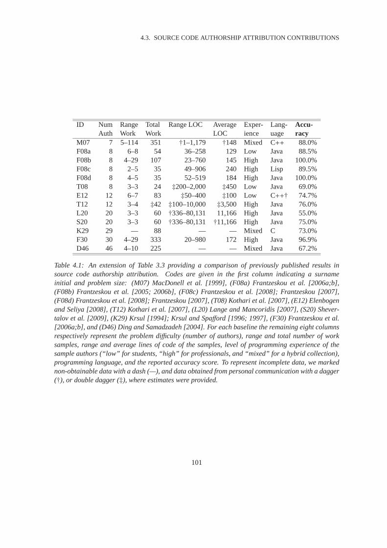
4.3. SOURCE CODE AUTHORSHIP ATTRIBUTION CONTRIBUTIONS
ID Num Range Total Range LOC Average Exper- Lang-Accu-Auth Work Work LOC ience uage racy
M07 7 5–114 351 †1–1,179 †148 Mixed C++ 88.0%F08a 8 6–8 54 36–258 129 Low Java 88.5%F08b 8 4–29 107 23–760 145 High Java 100.0%F08c 8 2–5 35 49–906 240 High Lisp 89.5%F08d 8 4–5 35 52–519 184 High Java 100.0%T08 8 3–3 24 ‡200–2,000 ‡450 Low Java 69.0%E12 12 6–7 83 ‡50–400 ‡100 Low C++† 74.7%T12 12 3–4 ‡42 ‡100–10,000 ‡3,500 High Java 76.0%L20 20 3–3 60 †336–80,131 11,166 High Java 55.0%S20 20 3–3 60 †336–80,131 †11,166 High Java 75.0%K29 29 — 88 — — Mixed C 73.0%F30 30 4–29 333 20–980 172 High Java 96.9%D46 46 4–10 225 — — Mixed Java 67.2%
Table 4.1: An extension of Table 3.3 providing a comparison of previouslypublished results insource code authorship attribution. Codes are given in the first column indicating a surnameinitial and problem size: (M07) MacDonell et al. [1999], (F08a) Frantzeskou et al. [2006a;b],(F08b) Frantzeskou et al. [2005; 2006b], (F08c) Frantzeskou etal. [2008]; Frantzeskou [2007],(F08d) Frantzeskou et al. [2008]; Frantzeskou [2007], (T08) Kothari et al. [2007], (E12) Elenbogenand Seliya [2008], (T12) Kothari et al. [2007], (L20) Lange and Mancoridis [2007], (S20) Shever-talov et al. [2009], (K29) Krsul [1994]; Krsul and Spafford [1996; 1997], (F30) Frantzeskou et al.[2006a;b], and (D46) Ding and Samadzadeh [2004]. For each baseline the remaining eight columnsrespectively represent the problem difficulty (number of authors), range and total number of worksamples, range and average lines of code of the samples, level of programming experience of thesample authors (“low” for students, “high” for professionals, and “mixed” for a hybrid collection),programming language, and the reported accuracy score. To represent incomplete data, we markednon-obtainable data with a dash (—), and data obtained from personal communication with a dagger(†), or double dagger (‡), where estimates were provided.
101

CHAPTER 4. BENCHMARKING PREVIOUS CONTRIBUTIONS
are reimplemented and then evaluated using the same test collections. We explainthis methodology
and the results obtained in the remaining sections of this chapter.
4.4 Benchmarking Methodology
The eight approaches above were implemented between 1994 [Krsul, 1994] and 2009 [Shevertalov
et al., 2009] using either custom-built programs or off-the-shelf software. Many decisions were
needed in reimplementing this previous work. For Frantzeskou et al. [2006a], we were required
to make some carefully considered decisions about the choice of n-gram length and profile length
from their recommendations that spanned multiple publications. For the metric-based contributions,
we were required to make some decisions about the reimplementation of potentiallythousands of
software measurements and a choice of common framework for the classification algorithms. We
review the Frantzeskou reimplementation decisions first in Section 4.4.1, followed by the metric-
based reimplementation decisions in Section 4.4.2. The remaining methodology thatis common to
all approaches is then given in Section 4.4.3.
4.4.1 Reimplementation of Frantzeskou Approach
The choice of n-gram lengthn and profile lengthL were the main considerations for the reimple-
mentation of the Frantzeskou work. As discussed in Section 4.3.4, valuesL = 2,000 andn= 6 were
common recommendations, so these values were selected. These values were chosen for the initial
benchmark only, and we note that the Frantzeskou work is revisited later in Section 7.2 (p. 175).
For generating the profiles, we used the Text::NGrams software [Keselj, 2008] as per the previous
work and truncated the samples atL = 2,000. After that, only join operations are needed to determine
the number of n-grams in common between the query and author profiles.
4.4.2 Reimplementation of Metric-Based Approaches with Weka
For the metric-based approaches, we had many classification algorithms to test, so the Weka machine
learning toolkit [Witten and Frank, 2005] version 3.5.8 was chosen to be a common framework. Three
of the prior contributions already used Weka, which we repeated, and in the other cases we chose the
closest available classification algorithm in Weka.
First, since Elenbogen and Seliya [2008] also used Weka for a C4.5 decision tree implementation,
we choose theweka.classifiers.trees.J48Weka classification algorithm implementation. Other prior
contributions that used Weka were a Bayesian Network classifier [Kothari et al., 2007] for which
102
4.4. BENCHMARKING METHODOLOGY
we chose theweka.classifiers.bayes.NaiveBayesimplementation, a Voting Feature Interval classi-
fier [Kothari et al., 2007] for which we chose theweka.classifiers.misc.VFIimplementation, and a
nearest neighbour classifier [Shevertalov et al., 2009] for which we chose theweka.classifiers.lazy.IB1
implementation.
Other baselines were not previously implemented in Weka, so alternatives were sought. We im-
plemented the nearest neighbour search of Lange and Mancoridis [2007] asweka.classifiers.lazy.IB1.
For the case-based reasoning model implemented by MacDonell et al. [1999] in the IDENTIFIED
package [Gray et al., 1998], we chose theweka.classifiers.lazy.IBkclassifier. Rodriguez et al. [2006]
noted the similarity between a variation named the connectionist fuzzy case-based reasoning model
and the k-nearest neighbour classifier: “the Connectionist Fuzzy Case-Based Reasoning model was
compared with a closely related method: the standard k-NN classifier (IBk in the Weka package)”.
We also chose twenty nearest neighbours for our implementation (k = 20) as the defaultk = 1 is
synonymous with theweka.classifiers.lazy.IB1classifier above. Usingk = 20 represents 33% of the
instances for one run of Coll-T and a lower portion for the other collections. This was the only
occasion where we deviated from the default Weka classifier parameters.
For the neural network classifier used in the work by MacDonell et al. [1999], we selected the
weka.classifiers.functions.MultilayerPerceptronclassifier. Widrow and Lehr [1990] described the per-
ceptron rule as one of the first neural network implementations first published in 1960.
To represent discriminant analysis as implemented by Krsul and Spafford [1997], MacDonell
et al. [1999], and Ding and Samadzadeh [2004], we used regressionanalysis. Meyers et al. [2005]
commented on the similarity of logistic regression (a form of regression analysis) to discriminant
analysis: “Discriminant function analysis is similar to logistic regression in that we use it to develop a
weighted linear composite to predict membership in two or more groups.” In Weka, several regression
classifiers are implemented includingweka.classifiers.meta.ClassificationViaRegression, which we
select for our baseline comparison.
Additional steps were needed for reimplementing the Kothari et al. [2007] work. This involved
training separate classification models for each author of each run and generating confidence scores
so that these scores could be pooled and ranked. A summary of all classification algorithms is given
in Table 4.2.
The remaining work required the exhaustive reimplementation of the softwaremetrics that ap-
peared in the seven metric-based contributions. We collapsed the metric classes from the three con-
tributions from Drexel University by Kothari et al. [2007], Lange andMancoridis [2007], and Shev-
ertalov et al. [2009], as there is much overlap in the metric classes. The setof eighteen metric classes
by Lange and Mancoridis [2007] was the most comprehensive, as the contribution by Kothari et al.
103

CHAPTER 4. BENCHMARKING PREVIOUS CONTRIBUTIONS
Contribution Classifier Weka ImplementationKrsul and Spafford [1997] Regression Analysis meta.ClassificationViaRegressionMacDonell et al. [1999] Case-Based Reasoninglazy.IBkMacDonell et al. [1999] Neural Network functions.MultilayerPerceptronMacDonell et al. [1999] Regression Analysis meta.ClassificationViaRegressionDing and Samadzadeh [2004] Regression Analysis meta.ClassificationViaRegressionKothari et al. [2007] Bayesian Network bayes.NaiveBayesKothari et al. [2007] Voting Feature Intervalsmisc.VFILange and Mancoridis [2007] Nearest Neighbour lazy.IB1Elenbogen and Seliya [2008] C4.5 Decision Tree trees.J48Shevertalov et al. [2009] Nearest Neighbour lazy.IB1
Table 4.2: List of all Weka classifiers used in this thesis. Note that the Weka implementations allbegin with the common “weka.classifiers.” prefix.
[2007] only had two new classes out of six, and the four classes contributed by Shevertalov et al.
[2009] was a strict subset of those by Lange and Mancoridis [2007].
We note that some recommendations were given in the literature that subsets ofsome metric sets
generated more accurate results than the full sets. Krsul [1994] gave multiple recommendations con-
cerning the best metric subset without providing a recommendation for the best overall subset. Lange
and Mancoridis [2007] also gave multiple recommendations concerning the use of the top-ranked au-
thor for attribution or longer lists. Additionally, Ding and Samadzadeh [2004]reported results from
a subset without publishing the final list. Given the imprecise details concerning the composition of
such subsets, we simply use the full sets of published metrics in these cases.
Therefore, we now say that there aresix feature sets for the metric-based contributions, and we
refer to the metric class contributions from Drexel University with the Langeand Mancoridis [2007]
citation from now on since their work represents most of the metric classes. The full metric sets are
documented in Appendix C.
Other decisions for implementation of the metrics are also described in AppendixC. This discus-
sion highlights metrics with difficult or impractical implementation requirements, language-specific
content, modifications that were required to avoid previously unconsidered error scenarios, and the
metrics that appear in multiple studies. Excluding the duplicates, we have reimplemented 172 metrics
altogether.
4.4.3 Methodology Common to All Approaches
We chose the ten-class problem for reporting our results. This was an arbitrary decision, but one
that is kept consistent throughout this thesis such that results between experiments can be easily
104

4.4. BENCHMARKING METHODOLOGY
compared. One exception is given later in Section 6.1.1 (p. 136). After randomly selecting all samples
by ten authors for a run, we can process more classification decisions byrepeating this many times,
which increases the statistical power of the experiments. All previous contributions in source code
authorship attribution have generally used modest collections, where the whole collection was used
at once for the experiments. This design limits statistically significant trends thatmay be observed.
With 1,597 samples in Coll-A, one run using this collection will contain about 10% of the col-
lection or about 160 samples. For Coll-A, a full experiment consists of100 runsor about 16,000
samples. The exact number of results depends on the authors that make upeach run.2 For the other
collections, we processed 250 runs for Coll-T, 150 runs for Coll-P, and 250 runs for Coll-J, so that
similar numbers of results would be available for comparison between collections.
We expect there to be some overlap between the authors chosen for eachrun, however it is ex-
tremely unlikely that any two runs in an experiment are identical. Using Coll-A as an example, there
are(
10010
)
≈ 1.73×10¹³ possible author subsets for selection for the one-in-ten problem, as explained
in Section 3.3. Duplication is extremely unlikely since, for example, we are using100 randomly
generated subsets for Coll-A.
We also consistently use a leave-one-out cross validation experiment design to maximise the
amount of training data per author. This was done using the command-line version of Weka where
we set the number of folds parameter to match the number of instances of eachrun. We considered the
Weka experimenter module with its graphical user interface, which makes it easy to queue multiple
classifiers and datasets. However, this Weka module does not accommodatea varying number of
folds as the interface only accepts constant input for this parameter, which makes leave-one-out cross
validation experiments cumbersome for our data.
Finally, we mention that we use accuracy as the sole measure for reporting our results, since this
thesis has a very large number of experiments. Use of a second measure such as error rates becomes
important in binary classification, for example, where the naive baseline is 50% accuracy assuming
that the number of samples in each class is equal.
In summary, it is clear that there is little agreement between the feature sets andclassification
algorithms in the previous studies. However, benchmarking them against one another using our
framework will allow the formulation of a baseline. The results of this work follow in Section 4.5.2Coll-T is an exception as it has exactly six samples per author.
105
CHAPTER 4. BENCHMARKING PREVIOUS CONTRIBUTIONS
4.5 Benchmarking Results
Results for the baseline reimplementations are shown in Figure 4.4. It is clear that some collections
represent more difficult problems than others, since the highest accuracy scores were generally for
Coll-P first, Coll-J second, Coll-A third, and Coll-T fourth. This observation is reiterated with
the average scores obtained for each set of twelve bars, which were 63.01%, 59.92%, 49.26%, and
42.33% respectively.
The results shown in Figure 4.4 demonstrate that the Frantzeskou approach (bars marked ‘f’) is
the most effective for all collections, with 66.40% accuracy for Coll-A, 67.57% for Coll-T, 85.74%
for Coll-P, and 82.96% for Coll-J. These scores therefore form the benchmark for our Information
Retrieval approach presented next in Chapter 5.
With the exception of the results for Lange and Mancoridis [2007], we notethat the scores
achieved are much lower than those summarised in Table 4.1. We note that this is adifficult compari-
son to make given that the results for the previous methods were obtained using different collections.
However, we suspect that overfitting may account for some of the differences given the generally
small collections that were used in the previous work.
When repeating experiments as necessary, we found that successiverepetitions of our multi-run
experiment design generally caused our results to vary by around 0.1% inaccuracy. We note that this
observation is an estimate only. This could be improved by reporting the standard deviation or vari-
ance, however a large number of multi-run experiments would be required,which is impractical given
that each individual multi-run experiment is large. Nevertheless, around0.1% variation accuracy was
rarely sufficient to change any key recommendation from our experiments.
4.6 Summary
In this chapter, we first reviewed all prior contributions from related research areas such as plagiarism
detection, genre classification, and natural language authorship attribution. We then described in
detail the metrics, classification algorithms, and general approaches of thesource code authorship
attribution contributions from eight research efforts. Following this, we reimplemented and evaluated
the prior work on large collections to verify the state-of-the-art and create reliable benchmarks for
our own contributions. We identified that the leading baseline is the work usingprofiles of byte-
level n-grams by Frantzeskou et al. [2005]. Next, in Chapter 5 we present the development of our
information retrieval prototype for source code authorship attribution.
106

4.6. SUMMARY
a b c d e f g h i j k l
Comparison of Baseline Approaches
Contributions ‘a’ to ‘l’ (described below)
Acc
urac
y (%
)
0
10
20
30
40
50
60
70
80
90
100
Coll−AColl−TColl−PColl−J
Figure 4.4: Comparison of all reimplemented prior contributions:(a) Krsul [1994] (regression anal-ysis and 42 features),(b) MacDonell et al. [1999] (k-nearest neighbour and 26 features),(c) Mac-Donell et al. [1999] (neural network and 26 features),(d) MacDonell et al. [1999] (regressionanalysis and 26 features),(e) Ding and Samadzadeh [2004] (regression analysis and 56 features),(f) Frantzeskou et al. [2006a] (simplified profile intersection (L= 2,000) and byte-level 6-grams),(g) Lange and Mancoridis [2007] and colleagues (nearest neighbour and 56 features),(h) Langeand Mancoridis [2007] and colleagues (Bayesian network and 56 features), (i) Lange and Man-coridis [2007] and colleagues (voting feature intervals and 56 features),(j) Kothari et al. [2007](Bayesian network and 50 features per author),(k) Kothari et al. [2007] (voting feature intervalsand 50 features per author), and(l) Elenbogen and Seliya [2008] (decision tree and 6 features).
107

CHAPTER 4. BENCHMARKING PREVIOUS CONTRIBUTIONS
108

Chapter 5
Applying Information Retrieval
Our review of previous contributions in Chapter 4 has identified eight approaches in source code au-
thorship attribution with published empirical results. Seven of these were metric-based approaches,
and the eighth approach used coordinate matching on n-grams. Our reviewof the published empir-
ical results suggested that the coordinate matching approach was the most accurate, and our bench-
marking experiment confirmed this finding when all previous approaches were reimplemented and
evaluated using our collections described in Chapter 3.
With a single non-metric approach providing the most accurate scores of allprevious approaches,
an obvious next step is to try other non-metric approaches. In this chapter, we introduce ourinfor-
mation retrieval approach. This approach was initially motivated by the application of information
retrieval to source code plagiarism detection by Burrows et al. [2006].
In Section 5.1, we introduce our seven-step methodology comprising collection construction,
anonymisation, tokenisation, n-gram construction, indexing, querying, and measuring accuracy. Sec-
tion 5.2 gives results of initial experiments to identify a suitable n-gram size andsimilarity measure
for our initial model containing programming language operator and keyword features. We provide
a second increment of our model in Section 5.3 using a revised feature setchosen empirically. In
Section 5.4, we provide our first classification results, which replaces theprevious results based on
reciprocal rank and average precision measurements, which were simplyused to indicate the quality
of the ranked lists. The work in Section 5.5 explores the accuracy and efficiency trade-off of two
index construction methods. Finally, we conclude this chapter in Section 5.6 witha summary of the
contribution and a link to the chapter that follows.
109

CHAPTER 5. APPLYING INFORMATION RETRIEVAL
5.1 Methodology
To determine the author of a document in our information retrieval approachto authorship attribution,
we treat the document as a search engine query — thequery document, written by thequery author—
on an indexed collection with known authors. Our approach produces a list of all documents in the
collection ranked by estimated similarity to the query document. Ideally, all documents by the query
author would appear at the top of the ranked list, followed by all other documents.
Specifically, the methodology follows seven steps. The first two steps concern collection con-
struction, which are common to authorship attribution in general. The next four steps concern our
information retrieval methodology. Then the final step is evaluation. The steps are as follows:
1. Construct a collection (or collections).
2. Anonymise the data by renaming files and directories, and removing commentsand string
literals from the source code.
3. Tokenise stylistic features from the source files, such as operators and keywords.
4. Convert each token stream into an n-gram representation by sliding a window of sizen one po-
sition at a time across the token stream. Therefore, a token stream of lengtht tokens generates
t−n+1 n-grams.
5. Index all n-gram samples belonging to ten randomly selected authors using the Zettair search
engine [Search Engine Group, 2009]. Repeat for many indexes.
6. Use contentious samples as queries against the indexed samples in each index, producing a
ranked list of the closest matching samples.
7. Measure effectiveness of the approach using MRR (mean reciprocal rank) and MAP (mean
average precision) on the ranked lists of results over many queries.
Next, we describe each of these steps in detail.
5.1.1 Collection Construction and Anonymisation
The first step in any authorship attribution work is collection construction. InChapter 3, we explained
how Coll-A, Coll-T, Coll-P, and Coll-J were constructed. In this chapter we only use Coll-A for
developing our approach to avoid overfitting concerns. Overfitting refers to tailoring an experiment
to produce good results for only limited data, and not applying more broadly.The other collections
110
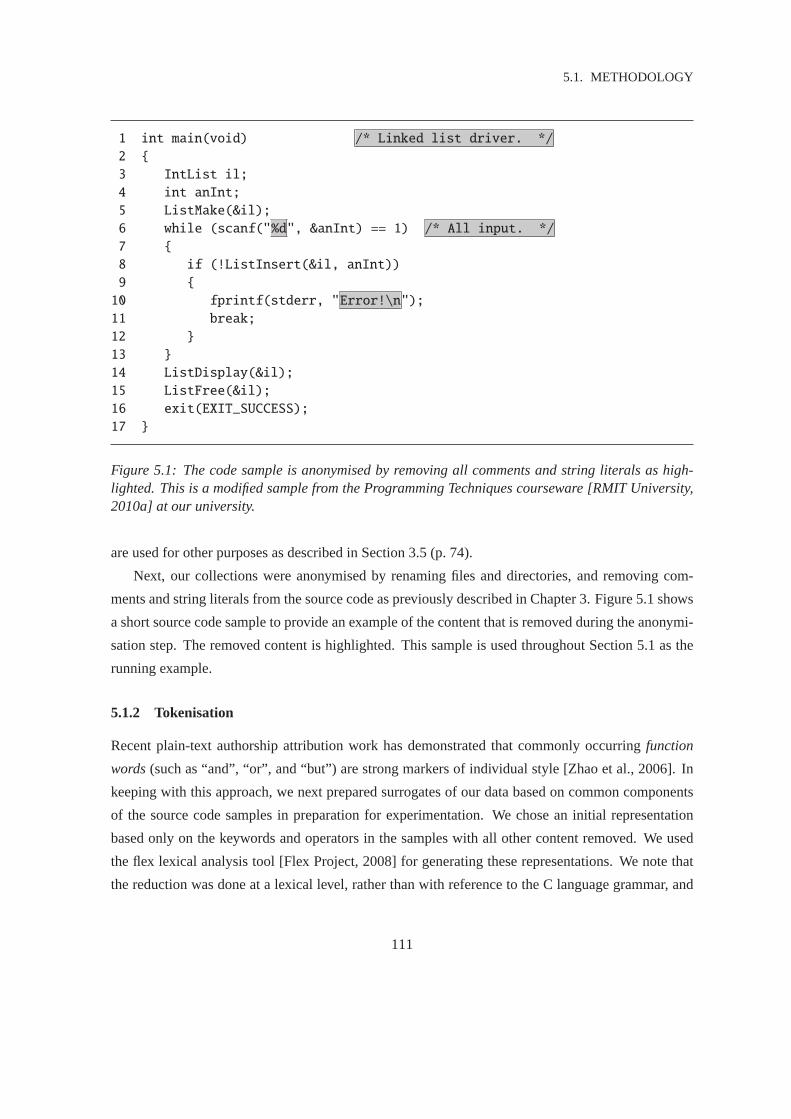
5.1. METHODOLOGY
1 int main(void) /* Linked list driver. */
2 {
3 IntList il;
4 int anInt;
5 ListMake(&il);
6 while (scanf("%d", &anInt) == 1) /* All input. */
7 {
8 if (!ListInsert(&il, anInt))
9 {
10 fprintf(stderr, "Error!\n");
11 break;
12 }
13 }
14 ListDisplay(&il);
15 ListFree(&il);
16 exit(EXIT_SUCCESS);
17 }
Figure 5.1: The code sample is anonymised by removing all comments andstring literals as high-lighted. This is a modified sample from the Programming Techniques courseware [RMIT University,2010a] at our university.
are used for other purposes as described in Section 3.5 (p. 74).
Next, our collections were anonymised by renaming files and directories, and removing com-
ments and string literals from the source code as previously described in Chapter 3. Figure 5.1 shows
a short source code sample to provide an example of the content that is removed during the anonymi-
sation step. The removed content is highlighted. This sample is used throughout Section 5.1 as the
running example.
5.1.2 Tokenisation
Recent plain-text authorship attribution work has demonstrated that commonlyoccurringfunction
words(such as “and”, “or”, and “but”) are strong markers of individual style [Zhao et al., 2006]. In
keeping with this approach, we next prepared surrogates of our data based on common components
of the source code samples in preparation for experimentation. We chose an initial representation
based only on the keywords and operators in the samples with all other content removed. We used
the flex lexical analysis tool [Flex Project, 2008] for generating these representations. We note that
the reduction was done at a lexical level, rather than with reference to the Clanguage grammar, and
111

CHAPTER 5. APPLYING INFORMATION RETRIEVAL
1 int main (void)
2 { Keywords
3 IntList il; Operators
4 int anInt;
5 ListMake(&il);
6 while (scanf("", &anInt) == 1)
7 {
8 if (!ListInsert(&il, anInt))
9 {
10 fprintf(stderr, "");
11 break;
12 }
13 }
14 ListDisplay(&il);
15 ListFree(&il);
16 exit(EXIT_SUCCESS);
17 }
Figure 5.2: The Figure 5.1 code sample is tokenised by extracting all keywords and operators ashighlighted. Operators that occur in pairs (such as parentheses) are only processed once.
so overloaded tokens are not treated differently in this thesis. For example, the C language asterisk
character (‘*’) is used for both multiplication and pointer dereferencing. Following our working
example, the keywords and operators that would be extracted from the Figure 5.1 example are shown
in Figure 5.2.
All possible C language operators and keywords that could be extractedfrom Coll-A are refer-
enced in Table D.1 (p. 230) in Appendix D.1
5.1.3 N-Gram Construction
The extracted operator and keyword features are next converted inton-grams. The n-gram representa-
tion is used since n-grams capture the context of tokens by including theirn−1 rightmost neighbours.
Prior to conversion to n-gram form, the tokens are first transformed into atwo-character al-
phabetic code as shown in the example in Figure 5.3. This format is chosen since document pre-
processing in search engine indexing (described next in Section 5.1.4) typically strips away most
characters that are not alphanumeric.
1Appendix D also has listings of operators and keywords relevant for Coll-P (C/C++ language) and Coll-J (Java lan-guage) in Tables D.2 (p. 231) and D.3 (p. 232) respectively. A separate table is not needed for Coll-T, as this collectionuses the same C language features as Coll-A.
112

5.1. METHODOLOGY
Figure 5.3 also shows the final transformation for our n-gram construction process. Here, the
twenty-six tokens extracted from the Figure 5.2 example are converted into twenty-one 6-grams. We
note that many candidate n-gram sizes are considered later in Section 5.2, and n = 6 is shown in
Figure 5.3 as an example only.
A problem arises when there are not enough tokens to make up at least one n-gram of the desired
length. In these cases, we had to remove those samples from further processing. This scenario
occurred for two samples in Coll-A, but not for the other collections.
5.1.4 Indexing
For our experiments, we reiterate that we chose to process many runs percollection, instead of having
one single large run, as explained in Section 4.4.3. That is, we chose not toindex the samples from
all 100 authors in Coll-A at once. Instead, we indexed all samples belonging to 10 random authors,
and then repeated this 100 times to generate 100 indexes. This design allows us to generate larger
result sets for analysis.
Figure 5.4 shows a partial example of an inverted index for one run. The lexicon contains all
unique n-grams that were derived in Figure 5.3, which have been sortedlexicographically. The
inverted lists contain the statistics about the occurrences of the n-grams in theindexed samples as
explained in Section 2.5.2 (p. 42).
The Zettair search engine was chosen for all indexing and querying tasks. Zettair is desirable as
it is open source, fast, highly scalable, and it supports ranked querying [Search Engine Group, 2009].
5.1.5 Querying
When querying, each of the approximately 160 samples from a run is treatedas a query in turn,
and is queried against the whole index. Figure 5.5 provides an example, where we have chosen to
represent the document identifier numbers using letters ‘A’ to ‘J’ to represent the ten authors, and a
natural number to indicate the sample number. Similarity between a query and each indexed sample
is computed with an information retrieval similarity measure such as those reviewed in Section 2.5.3
(p. 42). These are ranked in order of most similar to least similar to help us identify samples that are
of most interest stylistically.
5.1.6 Measuring Effectiveness
To evaluate the effectiveness of our work, we must measure the relative quality of the ranked lists
returned from the querying step in Section 5.1.5 above. We first measure effectiveness using the re-
113

CHAPTER 5. APPLYING INFORMATION RETRIEVAL
int ( void int ( & while ( ( , & == if ( ! ( & , ( , break ( & ( & (
⇓
1 2 3 4 5 6 7 8 9 10 11 12 13 14 15 16 17 18 19 20 21 22 23 24 25 26
in pa vo in pa am wh pa pa co am eq if pa no pa am co pa co br pa am pa am pa
⇓
1 in pa vo in pa am
2 pa vo in pa am wh
3 vo in pa am wh pa
4 in pa am wh pa pa
5 pa am wh pa pa co
6 am wh pa pa co am
7 wh pa pa co am eq
8 pa pa co am eq if
9 pa co am eq if pa
10 co am eq if pa no
11 am eq if pa no pa
12 eq if pa no pa am
13 if pa no pa am co
14 pa no pa am co pa
15 no pa am co pa co
16 pa am co pa co br
17 am co pa co br pa
18 co pa co br pa am
19 pa co br pa am pa
20 co br pa am pa am
21 br pa am pa am pa
Figure 5.3: The features extracted from the Figure 5.2 code sample are all converted into a two-character code. Then, a window of size six is moved across the token stream one position at a timeand the token-level 6-gram at each position is recorded. That is, a sequence of twenty-six unigramsis transformed into a sequence of twenty-one 6-grams. Note that the spaces within each 6-gramdisplayed are for readability only.
114

5.1. METHODOLOGY
amcopacobrpa
ameqifpanopa
amwhpapacoam
brpaampaampa
coameqifpano
cobrpaampaam
copacobrpaam
eqifpanopaam
ifpanopaamco
inpaamwhpapa
inpavoinpaam
nopaamcopaco
paamcopacobr
paamwhpapaco
pacoameqifpa
pacobrpaampa
panopaamcopa
papacoameqif
pavoinpaamwh
voinpaamwhpa
whpapacoameq
1: <A1,1>
1: <A1,1>
1: <A1,1>
1: <A1,1>
1: <A1,1>
1: <A1,1>
1: <A1,1>
1: <A1,1>
1: <A1,1>
1: <A1,1>
1: <A1,1>
1: <A1,1>
1: <A1,1>
1: <A1,1>
1: <A1,1>
1: <A1,1>
1: <A1,1>
1: <A1,1>
1: <A1,1>
Lexicon Inverted Lists
CollectionFrequency
DocumentFrequency
DocumentID
1: <A1,1>
1: <A1,1>
Figure 5.4: An example of an inverted index after the n-grams from Figure 5.3 have been inserted,assuming the sample is given the document identifier “A1”. The inverted index contains the lexiconof unique n-grams, and the inverted lists contain statistics about the occurrences of the n-grams inthe indexed data. The inverted lists for this one-sample index are trivial, but they generally increasein length as additional samples are indexed. Another example of an inverted index was given inFigure 2.6 (p. 43).
115

CHAPTER 5. APPLYING INFORMATION RETRIEVAL
A1
A1
... ... ... ...
...
...
...
... ...
...
A2 A3 A14 A15 A16
B14B3B2B1
C1 C2 C3 C14 C15 C16 C17
J15J14J3J2J1
Query
− − − − − − − − − − − − − − Indexed Content − − − − − − − − − − − − − −
Figure 5.5: Each indexed sample in a run is treated as a query in turn and evaluated for stylisticsimilarity using an information retrieval similarity measure. The results are ranked from most similarto least similar for identification of the samples that are of most interest. In thisexample, Sample A1is currently the query for comparison to the approximately 160 samples in a run forColl-A.
116
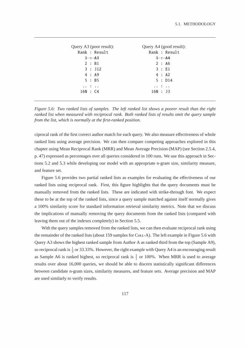
5.1. METHODOLOGY
Query A3 (poor result): Query A4 (good result):Rank : Result Rank : Result
1 : A3 1 : A4
2 : B1 2 : A6
3 : J12 3 : E1
4 : A9 4 : A2
5 : B5 5 : D14
.. : .. .. : ..
160 : C4 160 : J3
Figure 5.6: Two ranked lists of samples. The left ranked list shows a poorer result than the rightranked list when measured with reciprocal rank. Both ranked lists of results omit the query samplefrom the list, which is normally at the first-ranked position.
ciprocal rank of the first correct author match for each query. We also measure effectiveness of whole
ranked lists using average precision. We can then compare competing approaches explored in this
chapter using Mean Reciprocal Rank (MRR) and Mean Average Precision (MAP) (see Section 2.5.4,
p. 47) expressed as percentages over all queries considered in 100runs. We use this approach in Sec-
tions 5.2 and 5.3 while developing our model with an appropriate n-gram size,similarity measure,
and feature set.
Figure 5.6 provides two partial ranked lists as examples for evaluating the effectiveness of our
ranked lists using reciprocal rank. First, this figure highlights that the query documents must be
manually removed from the ranked lists. These are indicated with strike-through font. We expect
these to be at the top of the ranked lists, since a query sample matched againstitself normally gives
a 100% similarity score for standard information retrieval similarity metrics. Note that we discuss
the implications of manually removing the query documents from the ranked lists (compared with
leaving them out of the indexes completely) in Section 5.5.
With the query samples removed from the ranked lists, we can then evaluate reciprocal rank using
the remainder of the ranked lists (about 159 samples for Coll-A). The left example in Figure 5.6 with
Query A3 shows the highest ranked sample from Author A as ranked thirdfrom the top (Sample A9),
so reciprocal rank is13 or 33.33%. However, the right example with Query A4 is an encouraging result
as Sample A6 is ranked highest, so reciprocal rank is11 or 100%. When MRR is used to average
results over about 16,000 queries, we should be able to discern statisticallysignificant differences
between candidate n-gram sizes, similarity measures, and feature sets. Average precision and MAP
are used similarly to verify results.
117

CHAPTER 5. APPLYING INFORMATION RETRIEVAL
Finally, we note that this final step is forevaluatingour methodology. It should not be confused
with the tokenisation, n-gram construction, indexing, and querying steps,which formour approach
to source code authorship attribution.
5.2 N-Gram Size and Similarity Measure
For the first increment of our model, we were required to choose an appropriate n-gram size and
similarity measure. For the n-gram size, we explored sixteen representations of our document sur-
rogates usingn ∈ {1,2,4,6,8,10,12,14,16,18,20,30,40,50,70,90} to determine whether shorter or
longer patterns of tokens are good indicators of authorship.
For the similarity measure, we tested five different ranking schemes: Cosine [Witten et al., 1999],
Pivoted Cosine [Singhal et al., 1996], language modelling with Dirichlet smoothing [Zhai and Laf-
ferty, 2004], Okapi BM25 [Sparck-Jones et al., 2000a;b], and ourown scheme named Author1 [Bur-
rows and Tahaghoghi, 2007]. The first four ranking schemes were already incorporated into the
Zettair search engine, and we left the default free parameters unchanged. For Okapi BM25, we kept
b= 0.75,k1 = 1.2, andk3 = 1010. For Pivoted Cosine, we left the pivot value at 0.2. For the language
modelling approach with Dirichlet smoothing,µ was left set to 2,000. Finally, Cosine does not have
free parameters.
The fifth metric that we named Author1, is related to the relative frequency model by Shivakumar
and Garcia-Molina [1995] and Garcia-Molina et al. [1996]. This measure is based on the idea that
the term frequency in a query and a document should be similar when the query is a document. We
define this measure as:
Author1(Q,Dd) =∑
t∈Q∪Dd
1
min(∣
∣
∣ fq,t − fd,t∣
∣
∣ ,0.5) . (5.1)
In Table 5.1, we illustrate the effectiveness of each combination of the five similarity measures
and sixteen different values ofn. We found that the Okapi BM25 similarity measure combined
with 8-grams was most effective when measured in MRR (76.39%), and Okapi BM25 with 6-grams
was most effective when measured in MAP (26.70%). These results are underlined in Table 5.1.
We also examined the statistical significance of differences in MRR and MAP at the 95% con-
fidence level using a permutation test. A non-parametric test was needed, since the distribution of
reciprocal rank scores are very skewed towards 1.00. We chose thenull hypothesis to be “no differ-
ence from the most effective MRR or MAP result”, and tested 2-gram up to 14-gram results for all
five similarity measures. Pivoted Cosine with 8-grams (75.89%;p= 0.24) and Okapi BM25 with 6-
grams (75.59%;p = 0.06) were the next two highest MRR results and the differences were found
118

5.2. N-GRAM SIZE AND SIMILARITY MEASURE
Gram Similarity Measure MRR% Similarity Measure MAP%Size Au1 Cos Dir Oka P.Co Au1 Cos Dir Oka P.Co
1 51.53 59.41 23.36 42.66 28.49 17.05 19.85 12.22 17.72 13.312 65.80 68.44 28.33 67.34 53.33 20.73 22.50 12.98 23.24 18.254 72.00 74.10 53.43 75.52 72.79 23.91 25.10 19.33 26.00 23.706 73.85 74.42 59.42 75.59 74.70 25.71 25.82 20.44 26.70 25.528 75.49 74.94 61.17 76.39 75.89 24.96 24.65 19.58 25.61 25.0010 73.72 73.35 60.44 74.95 74.69 22.78 22.73 17.76 23.47 23.2512 74.17 73.45 61.39 74.95 74.55 21.57 21.42 16.95 22.01 21.7514 72.77 72.20 62.41 73.51 73.32 19.09 18.93 15.74 19.38 19.2816 71.63 71.12 63.55 72.20 72.25 16.81 16.71 14.73 16.98 16.9718 70.41 70.14 64.21 70.81 70.86 14.59 14.65 13.31 14.79 14.8120 67.96 67.92 64.48 68.27 68.33 13.36 13.41 12.66 13.53 13.5430 60.40 60.37 60.11 60.53 60.50 9.92 9.91 9.78 9.94 9.9540 54.48 54.40 54.39 54.48 54.48 8.51 8.51 8.49 8.52 8.5250 50.82 50.93 50.84 50.92 50.93 7.76 7.76 7.73 7.77 7.7670 45.98 46.00 45.78 46.04 46.03 6.44 6.45 6.43 6.45 6.4490 42.98 43.00 42.85 43.02 43.01 5.72 5.73 5.72 5.73 5.73
Table 5.1: Effect of varying the n-gram size and similarity measure. Five similarity measures aretested using sixteen different n-gram representations. The similarity measures are Author1 (Au1),Cosine (Cos), language modelling with Dirichlet smoothing (Dir), Okapi BM25 (Oka), and PivotedCosine (P.Co). Okapi BM25 with 8-grams for MRR and Okapi BM25 with 6-grams for MAP werethe most effective results and are underlined. Two further MRR results are renderedin boldface thatwere not statistically different from Okapi BM25 with 8-grams at the 95% confidence level.
119
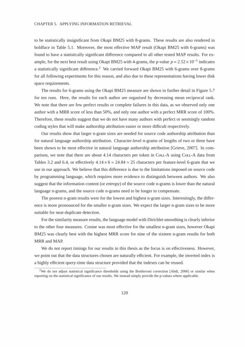
CHAPTER 5. APPLYING INFORMATION RETRIEVAL
to be statistically insignificant from Okapi BM25 with 8-grams. These results are also rendered in
boldface in Table 5.1. Moreover, the most effective MAP result (Okapi BM25 with 6-grams) was
found to have a statistically significant difference compared to all other tested MAP results. For ex-
ample, for the next best result using Okapi BM25 with 4-grams, the p-value p= 2.52×10⁻⁵ indicates
a statistically significant difference.2 We carried forward Okapi BM25 with 6-grams over 8-grams
for all following experiments for this reason, and also due to these representations having lower disk
space requirements.
The results for 6-grams using the Okapi BM25 measure are shown in further detail in Figure 5.7
for ten runs. Here, the results for each author are organised by decreasing mean reciprocal rank.
We note that there are few perfect results or complete failures in this data, as we observed only one
author with a MRR score of less than 50%, and only one author with a perfect MRR score of 100%.
Therefore, these results suggest that we do not have many authors withperfect or seemingly random
coding styles that will make authorship attribution easier or more difficult respectively.
Our results show that larger n-gram sizes are needed for source code authorship attribution than
for natural language authorship attribution. Character-level n-grams of lengths of two or three have
been shown to be most effective in natural language authorship attribution [Grieve, 2007]. In com-
parison, we note that there are about 4.14 characters per token in Coll-A using Coll-A data from
Tables 3.2 and 6.4, or effectively 4.14×6 = 24.84≈ 25 characters per feature-level 6-gram that we
use in our approach. We believe that this difference is due to the limitations imposed on source code
by programming language, which requires more evidence to distinguish between authors. We also
suggest that the information content (orentropy) of the source code n-grams is lower than the natural
language n-grams, and the source code n-grams need to be longer to compensate.
The poorest n-gram results were for the lowest and highest n-gram sizes. Interestingly, the differ-
ence is more pronounced for the smaller n-gram sizes. We expect the larger n-gram sizes to be more
suitable for near-duplicate detection.
For the similarity measure results, the language model with Dirichlet smoothing is clearly inferior
to the other four measures. Cosine was most effective for the smallest n-gram sizes, however Okapi
BM25 was clearly best with the highest MRR score for nine of the sixteen n-gram results for both
MRR and MAP.
We do not report timings for our results in this thesis as the focus is on effectiveness. However,
we point out that the data structures chosen are naturally efficient. For example, the inverted index is
a highly efficient query-time data structure provided that the indexes can be reused.
2We do not adjust statistical significance thresholds using the Bonferronicorrection [Abdi, 2006] or similar whenreporting on the statistical significance of our results. We instead simply provide the p-values where applicable.
120
5.2. N-GRAM SIZE AND SIMILARITY MEASURE
Author Number
Rec
ipro
cal R
ank
(%)
0 5 10 15 20 25 30 35 40 45 50
0
20
40
60
80
100
Author Number
Rec
ipro
cal R
ank
(%)
50 55 60 65 70 75 80 85 90 95 100
0
20
40
60
80
100
Figure 5.7: A sunflower plot showing the reciprocal rank scores for 100 authors from 10 runs of 10authors each. Results for the authors are sorted by MRR in descending order. The strokes projectingfrom each solid point (the “petals” of the “sunflowers”) represent additional points plotted at thesame positions.
121

CHAPTER 5. APPLYING INFORMATION RETRIEVAL
5.3 Selecting Source Code Features
Feature selection is non-trivial for authorship attribution and other classification problems. Work
by Oman and Cook [1990] alone provided 236 language-independent style rules compiled from 7
sources. It is clear that no researcher has explored all combinations of these exhaustively for the
purposes of source code authorship attribution given the number of combinations possible. Moreover,
the markers that are chosen in the literature are often arbitrary.
In this section, we improve our initial information retrieval model from Section 5.2 by introduc-
ing a more effective feature set. Supplanting the initial keyword and operator set, we first try remov-
ing unnecessary features in Section 5.3.1 using backwards feature selection to determine whether
removing bloat from our model improves effectiveness. Then we try the opposite and introduce in-
put/output keywords, function words, white space features, and literal features in Section 5.3.2, to
determine whether these can improve effectiveness.
5.3.1 Backwards Feature Selection
In this section, we perform backward feature selection to determine whether any keywords or oper-
ators can be omitted from the feature set without significantly reducing effectiveness. The goal is to
determine whether unnecessary noise caused by the use of all keywords and operators is adversely
impacting effectiveness. The set of keywords and operators that we used in our initial model are given
in Table D.1 (p. 230) from Appendix D.
We identify candidate features for removal based upon their total contributed weight to the Okapi
BM25 similarity measure. We implement backwards feature selection by progressively removing
features one at a time starting with the features with the smallest weight.
We found that backwards feature selection caused our MRR scores to degrade steadily. We
conjecture that this was caused by Coll-A having many small programs, since some of the programs
were reduced to no tokens after only a small number of features were removed. With no evidence
left to match query to document, such results were recorded as failures witha reciprocal rank of zero
assigned. We conclude that longer samples with more of the features present are needed for this type
of experiment to be effective. Therefore, we do not pursue backwards feature selection further.
5.3.2 Evaluating Feature Classes from the Literature
The Section 5.2 experiment used C language operators and keywords asan initial feature set. Then
in Section 5.3.1, we found that removing potentially unnecessary features did not help. Therefore,
we now consider introducing other types of features based on style guidelines from the literature.
122

5.3. SELECTING SOURCE CODE FEATURES
Much work is available that defines good programming style. For example, Cannon et al. [1997]
defined coding style guidelines such as commenting, white space, declarations, naming conventions,
and file organisation. Oman and Cook [1990] argued that many authors demonstrate personal pref-
erence, but suggested that empirical evidence is lacking to suggest thatvarious guidelines offer
improvements over alternatives to readability, portability, maintenance effort, and so on. There-
fore Oman and Cook [1990] argued that a common paradigm is needed. They collated programming
style guidelines from many sources and organised them in a taxonomy, whichwe use as a basis for
categorising style features in our work. The taxonomy contains three main categories.Typographic
stylerefers to all aspects of code that do not affect program execution, such as commenting, nam-
ing characteristics, and layout (spaces, tabs, and new lines). Next,control structure stylerefers to
flow control tokens that affect algorithm implementation decisions, such as operators, keywords, and
standard library functions. Finally,information structure stylerefers to the organisation of program
memory, input and output such as data structures, and input/output functions such asprintf and
scanf.
Based upon the above taxonomy, we create six classes of features for experimentation. From the
typographic style category, we experiment with white space features to represent the layout category,
and literal features to represent the naming characteristics category. Wedo not experiment with
comments, as we were required to strip these to comply with research ethics guidelines. From the
control structure category, we introduce standard header library keywords (such as constants, macros,
and function names) [Huss, 1997], which we collectively refer to asfunction words. We also retain
operators and keywords that were our starting point in Section 5.2. Fromthe information structure
style category, we experiment with standard header library keywords from stdio.h to represent
input/output functions [Huss, 1997]. We ensure that these are excluded from the function words
category described above. TheNULL and size_t tokens are also included that overlap with the
function words category. We do not experiment with data structure keywords, as we expect these
features to be infrequent. Moreover, there is some overlap with our literalscategory here. We provide
a summary of the number of tokens in each class in the top two rows of Table 5.2 with the complete
listings given in Tables D.4 (p. 233) and D.5 (p. 234) from Appendix D. The remainder of Table 5.2
shows the volume of tokens in Coll-A for each feature class. This data shows that white space
features dominate, followed by operators and literals. We also provide marked-up examples of all six
feature classes in Figure 5.8 based on our original code sample from Figure 5.1.
We experiment with all sixty-three (26−1) possible combinations of these feature classes, with
each combination forming afeature set. That is, we create 6-gram program representations with each
feature set in turn for our experiment design of 100 runs.
123

CHAPTER 5. APPLYING INFORMATION RETRIEVAL
1 int main(void)
2 {
3 IntList il;
4 int anInt;
5 ListMake(&il);
6 while (scanf("", &anInt) == 1)
7 {
8 if (!ListInsert(&il, anInt))
9 {
10 fprintf(stderr, "");
11 break;
12 }
13 }
14 ListDisplay(&il);
15 ListFree(&il);
16 exit(EXIT_SUCCESS);
17 }
(a)
1 int main(void)
2 {
3 IntList il;
4 int anInt;
5 ListMake(&il);
6 while (scanf("", &anInt) == 1)
7 {
8 if (!ListInsert(&il, anInt))
9 {
10 fprintf(stderr, "");
11 break;
12 }
13 }
14 ListDisplay(&il);
15 ListFree(&il);
16 exit(EXIT_SUCCESS);
17 }
(c)
1 int•main(void)¶
2 {¶
3 •••IntList•il;¶
4 •••int•anInt;¶
5 •••ListMake(&il);¶
6 •••while•(scanf("",•&anInt)•==•1)¶
7 •••{¶
8 ••••••if•(!ListInsert(&il,•anInt))¶
9 ••••••{¶
10 •••••••••fprintf(stderr,•"");¶
11 •••••••••break;¶
12 ••••••}¶
13 •••}¶
14 •••ListDisplay(&il);¶
15 •••ListFree(&il);¶
16 •••exit(EXIT_SUCCESS);¶
17 }¶
(e)
1 int main(void)
2 {
3 IntList il;
4 int anInt;
5 ListMake(&il);
6 while (scanf("", &anInt) == 1)
7 {
8 if (!ListInsert(&il, anInt))
9 {
10 fprintf(stderr, "");
11 break;
12 }
13 }
14 ListDisplay(&il);
15 ListFree(&il);
16 exit(EXIT_SUCCESS);
17 }
(b)
1 int main(void)
2 {
3 IntList il;
4 int anInt;
5 ListMake(&il);
6 while (scanf("", &anInt) == 1)
7 {
8 if (!ListInsert(&il, anInt))
9 {
10 fprintf(stderr, "");
11 break;
12 }
13 }
14 ListDisplay(&il);
15 ListFree(&il);
16 exit(EXIT_SUCCESS);
17 }
(d)
1 int main(void)
2 {
3 IntList il;
4 int anInt;
5 ListMake(&il);
6 while (scanf("", &anInt) == 1)
7 {
8 if (!ListInsert(&il, anInt))
9 {
10 fprintf(stderr, "");
11 break;
12 }
13 }
14 ListDisplay(&il);
15 ListFree(&il);
16 exit(EXIT_SUCCESS);
17 }
(f)
Figure 5.8: A code sample showing six feature classes for consideration in our model.(a) Operators.(b) Keywords.(c) Input/output tokens.(d) Function tokens.(e) White space tokens.(f) Literal tokens.
124

5.3. SELECTING SOURCE CODE FEATURES
WS Op Lit KW I/O Fn TotalFeatures 4 39 5 32 60 185 325Percent 1.23 12.00 1.54 9.85 18.46 56.92 100.00Tokens 8,109,257 1,495,730 1,409,749 384,718 143,691 76,355 11,619,500Percent 69.79 12.87 12.13 3.31 1.24 0.66 100.00
Table 5.2: Number of unique features in each feature class, and the distribution of tokens inColl-A.The six feature classes are white space tokens (WS), operators (Op), literal tokens (Lit), keywords(KW), input/output tokens (I/O), and function tokens (Fn).
The top six rows of Table 5.3 provide a summary of the top performing featuresets (all of which
have a statistically insignificant MRR from Feature Set 50 (the top row) usinga permutation test at the
p= 0.05 level). The bottom six rows show the performance of the six feature classes in isolation. As
can be seen, using feature sets that contain a single feature class leads toa poor ranking of documents
by the same author as the query, whereas selecting white space, operator, and keyword features
(Feature Set 50) leads to a high ranking of similarly authored documents.
Koppel et al. [2003] discussed that for text categorisation, “frequent but unstable features are
especially useful”, so we would expect the most frequent and diversefeature sets to be of most value.
White space features were the most prevalent as shown in Table 5.2 representing 69.79% of all tokens.
We believe they are especially useful as white space placement is a strong marker of programming
style. For example, the following two for-loop declarations are functionally equivalent, but the use of
white space can be helpful in distinguishing authorship:
for(i=0; i<limit; i++); for (i = 0; i < limit; i++);
In Figure 5.9 we plot the volume of tokens against the MRR score of each feature set. The feature
sets containing white space are separated (right hand side of six million tokens) from those that do
not (left hand side of six million tokens), as it is the class that contains the mostnumber of tokens
in the collection (refer to Table 5.2). Our results show that the most effective feature set without
white space features had a MRR score of 4.49% less than the most effective feature set. This is
a statistically significant difference as shown by a permutation test at the 95% confidence interval
using the reciprocal ranks of the queries (p= 2.20×10⁻¹⁶).
We also show each half of the graph separated into three smaller parts. In each half, the rightmost
part contains both operator and literal features, the middle part contains one of these, and the leftmost
part contains neither. The part with neither is clearly the least effective in both halves of the graphs,
further supporting the observation that using more features enhances ranking effectiveness, as these
are the two most frequent classes of tokens after white space.
125

CHAPTER 5. APPLYING INFORMATION RETRIEVAL
F. Set Op KW I/O Fn WS Lit MRR MAP50 Yes Yes Yes 82.28 41.3358 Yes Yes Yes Yes 82.20 40.3655 Yes Yes Yes Yes Yes 81.98 39.2251 Yes Yes Yes Yes 81.74 39.7454 Yes Yes Yes Yes 81.68 41.1362 Yes Yes Yes Yes Yes 81.61 39.90... ... ... ... ... ... ... ... ...32 Yes 74.78 26.19... ... ... ... ... ... ... ... ...16 Yes 69.40 20.33... ... ... ... ... ... ... ... ...01 Yes 65.73 23.1008 Yes 62.07 16.7904 Yes 56.98 9.9102 Yes 43.26 22.15
Table 5.3: Effectiveness of twelve of sixty-three tested feature sets sorted by MRR score. The sixfeature classes are operators (Op), keywords (KW), input/output tokens (I/O), function tokens (Fn),white space tokens (WS), and literal tokens (Lit) respectively. We omit the remaining fifty-one resultsfor brevity. These results shown demonstrate that operators, keywords, and white space featurestogether are strong markers of authorship. Note that the left-most columnis a numeric identifier thatwe refer to in the text to identify the feature set.
126

5.3. SELECTING SOURCE CODE FEATURES
0 1 2 3 4 5 6 7 8 9 10 11 12
40
45
50
55
60
65
70
75
80
85
Token Volume Versus MRR for All 63 Feature Sets
Millions of tokens
MR
R (
%) 1
2
3
4
56
7
8
9 10
11
12
1314
15
16
17
18
19
2021
22
23
2425
2627
2829
3031
3233
34 35
36 37
38 39
40
41
42 43
44 45
46 47
4849
50 51
5253
54 55
5657
5859
6061
62 63
Figure 5.9: Token volume plotted against classification effectiveness measured as MRR. The individ-ual feature sets are divided into six rough areas caused by the prevalence of some classes of featuresover others. White space tokens, operators, and literal tokens are the most dominant. Therefore thesix regions from left to right respectively represent: (1) none of these, (2) operators or literals, (3)operators and literals, (4) white space, (5) white space and operators,or white space and literals,(6) white space, operators, and literals. For example, the fifth region of the graph includes FeatureSet 50 as discussed in the text. This feature set has operators, keywords, and white space tokens, butno literals. Note that the boxed region in the top-right corner is expanded inFigure 5.10 for clarity.
127

CHAPTER 5. APPLYING INFORMATION RETRIEVAL
8.0 8.5 9.0 9.5 10.0 10.5 11.0 11.5 12.0
74
75
76
77
78
79
80
81
82
83
84
Token Volume Versus MRR for 29 of 63 Feature Sets
Millions of tokens
MR
R (
%)
3
7 11
14
15
18
19
22
23
26
2730
3134
3538
3942
43
46 47
50
515455
58
5962
63
Figure 5.10: An expanded view of the boxed region from the top-right corner of Figure 5.9 showingMRR scores for twenty-nine of the sixty-three evaluated feature sets. Feature Set 50 is the mosteffective with 82.28% MRR.
128
5.4. CLASSIFICATION
Key observations were made when inspecting the volumes of each individual token. For example,
the ratio of new lines to carriage returns was found to be 16:1. This suggests that at least one out
of sixteen samples was not developed in our predominantly Unix-based environment, and this gives
a useful authorship marker concerning choice of operating system forprogramming assignment de-
velopment. The white space and literal tokens were all found in large quantities, as the nine tokens
that make up these categories were all within the top fifteen when totalling the volume of each token.
Of the remaining token classes, the parenthesis was the most prevalent operator token,int was the
most prevalent keyword,NULL was the most prevalent input/output token, andstrlen was the most
prevalent function token.
In summary, in this section we have explored sixty-three feature sets, and we found that the white
space, operator, and keyword classes were most effective. In particular, this combination of classes
(named “Feature Set 50”) was also the most effective combination of all those evaluated. The MRR
score increased from 75.59% to 82.28% (+6.69%) and the MAP score increased from 26.70% to
41.33% (+14.63%) compared to the previous scores from Section 5.2. Therefore,this feature set is
carried forward for all experiments that follow.
5.4 Classification
The experiments in Sections 5.2 and 5.3 have used MRR and MAP to evaluate thequality of the
ranked lists. These scores have allowed us to make decisions for key parameters in our model,
such as choice of n-gram size, choice of information retrieval similarity measure, and choice of
feature set. Having made these decisions, the next step is to make actual authorship classification
decisions to measure the accuracy level of our model. In this section, we evaluate three methods for
deciding authorship, followed by a comparison of our accuracy scoresto the reimplemented baselines
presented in Chapter 4.
5.4.1 Overall Results
In this section, we evaluate three metrics for determining classification accuracy. Therefore, the MRR
and MAP measurements that were only used to compare the quality of ranked lists in Sections 5.2
and 5.3 are no longer used.
First, thesingle best resultmetric attributes authorship to the author of the top ranked document.
The proportion of times that this is correct is used to calculate overall accuracy. This metric is the
only one that uses asingle documentfrom the ranked list for the authorship decision.
129

CHAPTER 5. APPLYING INFORMATION RETRIEVAL
Sample Sample Similarity Classified Author Single Best ResultRank Author Score A 1.0
1 A1 0.8 B 0.02 B1 0.5 C 0.03 B2 0.5 Classified Author Average Scaled Score4 C1 0.5 A (0.8+ 0.2+ 0.2+ 0.2+ 0.2) / 5 = 0.325 B3 0.5 B (0.5+ 0.5+ 0.5+ 0.2) / 4 = 0.436 B4 0.2 C (0.5) / 1= 0.57 A2 0.2 Classified Author Average Precision8 A3 0.2 A (1/1 + 2/7 + 3/8 + 4/9 + 5/10) / 5 = 0.529 A4 0.2 B (1/2+ 2/3+ 3/5+ 4/6) / 4= 0.6110 A5 0.2 C (1/1) / 4 = 0.25
Table 5.4: A ranked list of ten samples (left) and how the single best result, average scaled score andaverage precision measurements vary depending on the order of samples in the ranked list and thesimilarity scores (right).
Next, theaverage scaled scoremetric uses the Okapi BM25 similarity scores returned by the
search engine. The scores are first normalised against the score from the top-ranked document,
which is otherwise not considered in the ranked list. Then the normalised scores for each author are
averaged, and authorship is assigned to the author with the highest average score. Overall accuracy
is again the proportion of times that this is correct. This is the only metric that usesthe absolute
similarity measurements of the search engine.
Finally with theaverage precisionmetric, we calculate the average precision for the documents of
each candidate author in turn, and assign authorship to the author with the highest average precision
score. Again, the proportion of times this is correct is used for calculating overall accuracy. This
metric is the only one that uses therelativesimilarity measurements of the search engine.
Table 5.4 provides example calculations of the three metrics on a dummy ranked list, comprising
samples from three authors named Author A, Author B, and Author C. This example demonstrates
scores that each metric would generate for the dummy ranked list. The authorwith the highest score
is classified as the correct author. Therefore according to the scoresshown, the query sample (not
shown) is classified as Author A for the single best result metric, Author B for the average precision
metric, and Author C for the average scaled score metric. Then accuracyis the proportion of times
that the classified author matches the actual author of the query sample.
We present our classification experiment results in Table 5.5. When using the “single best result”
classification method, we correctly classified work in 76.78% of cases for the ten-class problem.
This is the best of our methods compared to “average scaled score” (76.47%, p= 0.52) and “average
130

5.4. CLASSIFICATION
Num Single Best Result Average Scaled Score Average PrecisionAuth Correct Percent Correct Percent Correct Percent
7 8,773/ 11,153 78.66% 8,795/ 11,153 78.86% 8,561/ 11,153 76.76%8 9,954/ 12,686 78.46% 9,977/ 12,686 78.65% 9,739/ 12,686 76.77%10 12,261/ 15,969 76.78% 12,212/ 15,969 76.47% 11,925/ 15,969 74.68%12 14,381/ 19,110 75.25% 14,127/ 19,110 73.92% 13,909/ 19,110 72.78%20 23,087/ 31,859 72.47% 21,885/ 31,859 68.69% 21,725/ 31,859 68.19%29 32,782/ 46,387 70.67% 30,210/ 46,387 65.13% 30,469/ 46,387 65.68%30 33,677/ 47,785 70.48% 30,864/ 47,785 64.59% 31,224/ 47,785 65.34%46 50,309/ 73,362 68.58% 44,723/ 73,362 60.96% 46,200/ 73,362 62.98%
Table 5.5: Overall comparison of the three classification methods. Varying problem sizes are shownincluding the ten-class problem that is largely used in our work, and other problem sizes from seven-class to forty-six-class that have been used by other researchers (see Table 3.3, p. 73).
precision” (74.68%,p = 1.23×10⁻⁵), but the difference was not statistically significant in the first
case as indicated.
In Table 5.5, we also present results for seven other problem sizes ranging from seven-class to
forty-six-class, which have been used in previous source code authorship attribution approaches, as
reviewed in Section 3.4 (p. 70). The motivation for repeating our experiment on the other problem
sizes is to consider whether the length of the ranked lists affects the three metrics evaluated. We
found that the “single best result” method was again most effective for the harder authorship attribu-
tion problems (twelve-class up to forty-six-class), however the “average scaled score” results were
marginally higher for the seven-class and eight-class problems by 0.20% and 0.21% respectively.
Most interestingly, the single best result metric produces the best results for the larger problem sizes,
possibly due to the other metrics being forced to process many potentially unhelpful results.
In summary, the “single best result” metric is most effective for most of the problem sizes consid-
ered, and we carry this forward for all experiments that follow. The other metrics are not used in the
remainder of this thesis. We also note that additional metrics could have been considered, but these
have been left for future work. In particular, a voting model could be implemented where the results
of multiple metrics are combined, and authorship is attributed to the author with the highest score for
the greatest number of metrics.
5.4.2 Comparing Accuracy to the Reimplemented Work
Figure 5.11 shows our ten-class result from Table 5.5 (using the single best result metric) against
the reimplemented baseline results from Section 4.5 for Coll-A. Our 76.78% classification accuracy
score is 10.38% above the next best accuracy score of 66.40% by Frantzeskou et al. [2006a]. We
131

CHAPTER 5. APPLYING INFORMATION RETRIEVAL
only show Coll-A results for now as this collection is used for developing our approach.More
improvements follow in Chapter 6, which resulted from our investigation of factors that affect the
accuracy of our approach. The full comparison is given later in Section7.1 (p. 173).
An interesting result from Figure 5.11 is the general drop in results from the other researchers
compared to those reported in their original publications as summarised in Table4.1. We have reim-
plemented the previous work as closely as possible as explained in Section 4.4, however the problem
sizes are of course different. This is demonstrated in Figure 5.11, which uses the ten-class problem
consistently, but Table 4.1 uses the problem sizes in the publications from seven-class to forty-six-
class. However, a surprising trend is that all of the larger problem size results in Table 4.1 are higher
than the ten-class results in Figure 5.11, with the exception of Lange and Mancoridis [2007]. The
discrepancy could be explained by the previous problems being easier based on the collections cho-
sen, or possible statistical anomalies from the use of modest collections. There is scope to further
explore this area by repeating the Figure 5.11 experiment for other problem sizes, but this remains as
future work, as the aim of this thesis is provide results consistently for the ten-class problem, given
the time requirements for each experiment. However, we briefly explore multipleproblem sizes in
Section 6.1.1.
5.5 Managing the Number of Indexes
When implementing our methodology described in Section 5.1, the query documents were left in our
inverted indexes, but later omitted from the result lists as shown in Figure 5.6.A consequence of this
decision is that the indexed query document tokens still play a part in the calculation of the Okapi
BM25 formula. Specifically, raw document frequency (ft), average document length (|Davg|), and the
number of documents (N) are affected.
However, the decision to leave the query document in the index was designed to improve the
efficiency of our index construction step and reduce disk space requirements. If the query document
is omitted, then the index for each query in a run will be different. Therefore, a run that normally
requires a single index will instead require approximately 160 indexes for Coll-A. Since the purpose
of an inverted index is to resolve queries efficiently, it is undesirable to make the most expensive step
approximately 160 times more expensive.
We decided to compare the accuracy scores of both approaches to ensure that our more efficient
choice did not adversely impact accuracy. For the more efficient option, we achieved 76.78% ac-
curacy for the one-in-ten classification problem, as shown previously in Figure 5.5 (12,261 queries
correct out of 15,969). For the less efficient option, we achieved a score of 76.52% accuracy (12,205
132

5.5. MANAGING THE NUMBER OF INDEXES
Burrows a b c d e f g h i j k l
Comparison of Our Work to Baseline Approaches
Burrows contribution and contributions ‘a’ to ‘l’ (described below)
Acc
urac
y (%
)
0
10
20
30
40
50
60
70
80
90
100
Figure 5.11: Accuracy score of our model compared with the accuracy scores of the reimple-mented prior contributions:(a) Krsul [1994] (regression analysis and 42 features),(b) MacDonellet al. [1999] (k-nearest neighbour and 26 features),(c) MacDonell et al. [1999] (neural networkand 26 features),(d) MacDonell et al. [1999] (regression analysis and 26 features),(e) Ding andSamadzadeh [2004] (regression analysis and 56 features),(f) Frantzeskou et al. [2006a] (simpli-fied profile intersection (L= 2,000) and byte-level 6-grams),(g) Lange and Mancoridis [2007] andcolleagues (nearest neighbour and 56 features),(h) Lange and Mancoridis [2007] and colleagues(Bayesian network and 56 features),(i) Lange and Mancoridis [2007] and colleagues (voting featureintervals and 56 features),(j) Kothari et al. [2007] (Bayesian network and 50 features per author),(k) Kothari et al. [2007] (voting feature intervals and 50 features per author), and(l) Elenbogen andSeliya [2008] (decision tree and 6 features).
133

CHAPTER 5. APPLYING INFORMATION RETRIEVAL
queries correct out of 15,950). We evaluated the significance of this difference using a Z-test for
the two proportions given. The p-value wasp = 0.59, and this very high p-value tells us that these
proportions are not significantly different.
With this result, we remark that it is satisfactory to use either of these methods, since in practice
the query document is available. In Chapter 6, we continue to use the efficient variation as we have
done in this chapter for exploring factors that affect accuracy of our information retrieval approach.
However, we switch to the less efficient option in Chapter 7, to be consistent with the methods used
to reimplement the baselines in this thesis. This final contribution chapter is the only chapter where
we benchmark the accuracy of our work to all previous contributions using all four of our collec-
tions, including our Coll-P and Coll-J benchmarking-only collections. Therefore, the final results
in Chapter 7 are the ones that should be considered definitive for the purposes of other researchers
benchmarking our work in the future.
5.6 Summary
In this chapter, we have presented our information retrieval model to source code authorship attribu-
tion. We have shown that combining modest n-gram sizes (n = 6) of operator, keyword, and white
space tokens with the Okapi BM25 similarity metric is very effective. We have also demonstrated
that leaving the query samples in the indexes does not adversely impact accuracy, but instead leads
to reduced index construction time and index disk space by a factor equal tothe number of samples
in one experiment run. Our authorship attribution accuracy score is 76.78% for the one-in-ten prob-
lem for Coll-A, which is more than 10% above the most effective baseline we have reimplemented.
Next, in Chapter 6 we investigate several factors that affect the accuracy of our approach including
the amount of training data, code quality, timestamps, and entropy.
134

Chapter 6
Effectiveness Parameters
In Chapter 5, we presented an information retrieval approach to sourcecode authorship attribution
using a search engine to index and query n-gram representations of source code samples. It remains
to be seen how our approach handles problems with variations to the number of authors, number
of samples per author, sample size, author stylistic strength, and sample timestampthat were not
explored in Chapter 5.
In this chapter, we explore each of these factors in turn for our approach. In Section 6.1, we
begin by exploring the effect of problem size concerning the number of authors, and the number of
samples per author. Next, we look at the effect of sample length on accuracy scores in Section 6.2.
We present some results for evaluating stylistic strength and its relationship withour accuracy scores
in Section 6.3. The remainder of the chapter concerns experiments using Coll-T to explore the effect
of timestamp and topic in Sections 6.4 and 6.5, and to identify the individual features that are the
strongest contributors towards making authorship decisions in Sections 6.6and 6.7. A summary of
this chapter is given in Section 6.8 with links to the chapter that follows.
6.1 Problem Size
An authorship attribution problem size concerns the total number of samples ina collection. These
samples can be divided in any number of ways concerning the number of authors, and the number
of samples per author. For example, a collection of 100 samples could be constructed from samples
belonging to 10 authors with 10 samples each, 5 authors with 20 samples each,or any other combi-
nation either stratified or otherwise. We next explore how our approach isaffected to variations in the
number of authors and number of samples per author.
135

CHAPTER 6. EFFECTIVENESS PARAMETERS
Number Accuracy Percentageof Our Method Zhao [2007]
Authors Okapi BM25 DecTr KNNei NNei Bayes BayNt KLD (µ = 10)2 89.18 77.1 84.6 85.5 85.1 86.0 89.73 85.51 70.5 74.6 76.0 77.5 79.5 83.94 83.20 63.1 70.6 71.6 69.9 75.8 79.95 81.35 58.9 66.2 69.5 66.4 71.7 76.210 76.78 — — — — — —20 72.86 — — — — — —50 68.38 — — — — — —100 65.89 — — — — — —
Table 6.1: Effect of modifying the number of authors compared with external benchmarks for natu-ral language authorship attribution. Our work is reported for 6-grams ofsource code tokens usingOkapi BM25 onColl-A. The Zhao [2007, Tables 3.10 and 4.7] benchmarks are for a subcollection ofthe TREC collection [Harman, 1995] comprising newswire articles from Associated Press. Functionwords were used as features, and the collection comprised fifty documentsper author. The classifiersevaluated by Zhao [2007] comprised the decision tree (DecTr), k-nearest neighbour (KNNei), near-est neighbour (NNei), Naive Bayes (Bayes), Bayesian Network (BayNt) and Kullback-Leibler Diver-gence (KLD) classification methods — all abbreviations of this form are summarised in Appendix A.3(p. 209). Results for ten-class problems sizes and above were not published by Zhao [2007], and aremarked with dashes (—). Permission to reproduce the Zhao [2007] datawas provided by author YingZhao on 12 August 2010.
6.1.1 Number of Authors
The results presented so far were for a 10-class problem, so we next explored problem sizes from 2-
class to 100-class. These results are presented in Table 6.1 for eight problem sizes. The results show
that our previously reported 10-class result (78.78%) degrades by 10.89% when increased by a factor
of 10 to 100-class. We expect results to continue to degrade for even larger problems.
The compromise between accuracy and the number of authors problem sizeis an unavoidable
trade-off. To demonstrate this, we have repeated previously published results by Zhao [2007] side by
side with ours in Table 6.1 for their reported problem sizes. These results also show degradation as
the number of authors is increased.
The previous source code authorship attribution research reviewed in Section 4.3 (p. 90) did not
include similar experiments showing rates of degradation similar to Table 6.1, so itis difficult to make
remarks about whether our level of degradation is reasonable. The best comparison we could find was
the natural language authorship attribution results by Zhao [2007], as reproduced in Table 6.1. The
work by Zhao [2007] was reviewed in detail in Section 4.2 (p. 85), and thisbody of work is perhaps
136

6.1. PROBLEM SIZE
one of the most comprehensive benchmarking studies for natural language authorship attribution.
We stress that no absolute comparison of our results and the natural language authorship attribu-
tion baseline in Table 6.1 is suitable, as there are many different experiment parameters that could
not be reproduced. The collections are not the same, as Zhao [2007] used a subcollection of the
TREC [Harman, 1995] collection using newswire articles from Associated Press. Moreover, our col-
lection was not large enough to have fifty samples per author as used in the natural language work.
Furthermore, we have not changed our leave-one-out cross validation experiment design decision to
ten-fold as used in the natural language work, to allow our results in Table 6.1 to be compared easily
to the other results in this thesis.
Putting all the above comparison problems aside, it is perhaps most appropriate to compare the
rate of degradation for the problem size results reported by both contributions. Our work degraded
from 89.18% to 81.35% when the problem size increased from two-class to five-class, which was a
loss of 7.83%. In comparison, the natural language scores degraded by between 13.9% and 21.4%
depending on the classification algorithm.1 This included their best-performing Kullback-Leibler
Divergence (KLD) classification algorithm, which degraded by 16.0%, which is more than twice the
rate of ours. These results show that our work is promising for dealing withlarge numbers of authors.
Despite this pleasing result, any decline in accuracy in general is still undesirable. A method
for managing this problem may be to publish confidence scores for each classification decision, in
addition to just declaring the most likely author. For example, if a classification outcome was that
Author A was correct with 51% confidence, and that Author B was correct with 49% confidence for a
two-class problem, then Author A would be classified as correct, even though we would be incorrect
on 49% of the occasions. These borderline classification decisions are unhelpful, and it may be more
appropriate to simply declare these as “unsure”. Therefore a good wayto advance this idea is to
simply declare some classifications as “unsure” for confidence scores below an established threshold.
This idea can be explored for future work in the field of source code authorship attribution, although
there is some previous work in natural language authorship attribution in this area, such as the paper
by Koppel et al. [2009].
6.1.2 Number of Samples per Author
We next explored modifying the number of samples per author. We could onlydecrease the number
of samples per author compared with previous experiments, as we were already using all samples
by each author. The full amount is sixteen samples per authoron averagefor Coll-A, with the
exact number varying between fourteen and twenty-six. We also explored twelve, eight, four, and
1Results from Zhao [2007] are only reported to one decimal place.
137
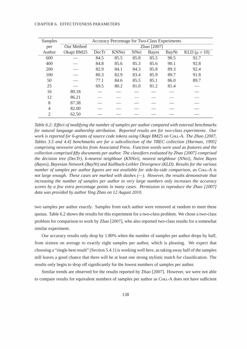
CHAPTER 6. EFFECTIVENESS PARAMETERS
Samples Accuracy Percentage for Two-Class Experimentsper Our Method Zhao [2007]
Author Okapi BM25 DecTr KNNei NNei Bayes BayNt KLD (µ = 10)600 — 84.5 85.5 85.8 85.5 90.5 92.7400 — 84.8 85.6 85.3 85.6 90.1 92.8200 — 82.9 84.1 84.3 85.8 89.3 92.4100 — 80.3 82.9 83.4 85.9 89.7 91.850 — 77.1 84.6 85.5 85.1 86.0 89.725 — 69.5 80.2 81.0 81.2 81.4 —16 89.18 — — — — — —12 86.21 — — — — — —8 87.38 — — — — — —4 82.00 — — — — — —2 62.50 — — — — — —
Table 6.2: Effect of modifying the number of samples per author compared with external benchmarksfor natural language authorship attribution. Reported results are for two-class experiments. Ourwork is reported for 6-grams of source code tokens using Okapi BM25on Coll-A. The Zhao [2007,Tables 3.5 and 4.4] benchmarks are for a subcollection of the TREC collection [Harman, 1995]comprising newswire articles from Associated Press. Function words were used as features and thecollection comprised fifty documents per author. The classifiers evaluatedby Zhao [2007] comprisedthe decision tree (DecTr), k-nearest neighbour (KNNei), nearest neighbour (NNei), Naive Bayes(Bayes), Bayesian Network (BayNt) and Kullback-Leibler Divergence(KLD). Results for the variousnumber of samples per author figures are not available for side-by-side comparison, asColl-A isnot large enough. These cases are marked with dashes (—). However, the results demonstrate thatincreasing the number of samples per author to very large numbers onlyincreases the accuracyscores by a few extra percentage points in many cases. Permission to reproduce the Zhao [2007]data was provided by author Ying Zhao on 12 August 2010.
two samples per authorexactly. Samples from each author were removed at random to meet these
quotas. Table 6.2 shows the results for this experiment for atwo-classproblem. We chose a two-class
problem for comparison to work by Zhao [2007], who also reported two-class results for a somewhat
similar experiment.
Our accuracy results only drop by 1.80% when the number of samples per author drops by half,
from sixteen on average to exactly eight samples per author, which is pleasing. We expect that
choosing a “single best result” (Section 5.4.1) is working well here, as taking away half of the samples
still leaves a good chance that there will be at least one strong stylistic match for classification. The
results only begin to drop off significantly for the lowest numbers of samples per author.
Similar trends are observed for the results reported by Zhao [2007]. However, we were not able
to compare results for equivalent numbers of samples per author as Coll-A does not have sufficient
138
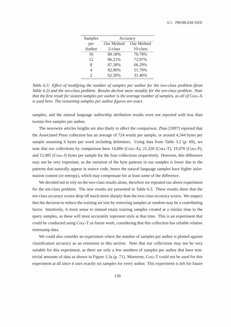
6.1. PROBLEM SIZE
Samples Accuracyper Our Method Our Method
Author 2-class 10-class16 89.18% 76.78%12 86.21% 72.97%8 87.38% 66.29%4 82.00% 51.78%2 62.50% 31.40%
Table 6.3: Effect of modifying the number of samples per author for the two-class problem (fromTable 6.2) and the ten-class problem. Results decline more steadily for the ten-class problem. Notethat the first result for sixteen samples per author is the average numberof samples, as all ofColl-Ais used here. The remaining samples per author figures are exact.
samples, and the natural language authorship attribution results were not reported with less than
twenty-five samples per author.
The newswire articles lengths are also likely to affect the comparison. Zhao [2007] reported that
the Associated Press collection has an average of 724 words per sample,or around 4,344 bytes per
sample assuming 6 bytes per word including delimiters. Using data from Table 3.2(p. 69), we
note that our collections by comparison have 14,806 (Coll-A), 21,320 (Coll-T), 19,478 (Coll-P),
and 15,985 (Coll-J) bytes per sample for the four collections respectively. However, thisdifference
may not be very important, as the variation of the byte patterns in our samples is lower due to the
patterns that naturally appear in source code, hence the natural language samples have higher infor-
mation content (or entropy), which may compensate for at least some of the difference.
We decided not to rely on the two-class results alone, therefore we repeated our above experiment
for the ten-class problem. The new results are presented in Table 6.3. These results show that the
ten-class accuracy scores drop offmuch more sharply than the two-class accuracy scores. We suspect
that the decision to reduce the training set size by removing samplesat randommay be a contributing
factor. Intuitively, it more sense to instead retain training samples created ata similar time to the
query samples, as these will most accurately represent style at that time. This is an experiment that
could be conducted using Coll-T as future work, considering that this collection has reliable relative
timestamp data.
We could also consider an experiment where the number of samples per author is plotted against
classification accuracy as an extension to this section. Note that our collections may not be very
suitable for this experiment, as there are only a few numbers of samples per author that have non-
trivial amounts of data as shown in Figure 3.3a (p. 71). Moreover, Coll-T could not be used for this
experiment at all since it uses exactly six samples for every author. This experiment is left for future
139

CHAPTER 6. EFFECTIVENESS PARAMETERS
Property Coll-A Coll-T Coll-P Coll-J(a) Mean Tokens 3,575 4,952 5,839 4,220(b) Mean LOC 830 1,108 984 667(c) (a)/(b) 4.31 4.14 5.93 6.33
Table 6.4: Collection properties for our collections: the mean number of feature-level tokens ex-tracted with our approach, the mean number of lines of code, and the ratiobetween these two num-bers.
work.
Finally, we remark that the results in this section do not make it clear how much training data
per author should be used, as there are many variables for consideration. We simply conclude that as
much training data as practical should be used.
6.2 Sample Length
We next explore the effects of varying query length towards the effectiveness of source code author-
ship attribution. That is, to record the query length in number of tokens against the accuracy scores.
This will allow us to investigate how effective source code authorship attribution is for trivial or
somewhat incomplete source code samples.
We also wanted a simple baseline for our reported results. Therefore, wedecided to compare the
best of our feature sets (Feature Set 50), to the average of all sixty-three feature sets. Feature Set 50
was chosen in Section 5.3 to be carried forward for all following experiments, as it was deemed to
produce highly accurate results. The goal is to show how the selection of our strong feature set can
increase accuracy particularly for the smallest queries.
We summarise the results for our query length investigation in Figure 6.1. Our results are par-
titioned into program lengths with intervals of 100 tokens initially (0–99, 100–199, 200–299, and
so on). Samples are then partitioned into intervals of 1,000 tokens for sampleswith 1,000 or more
tokens, given that we have fewer of these. The final partition is marked as 20,000, which represents
all programs with at least 20,000 tokens up to the maximum in Coll-A (95,889 tokens). Figure 3.4a
(p. 72) gave some indication of the actual distribution expressed as lines ofcode. When considering
the distribution in tokens instead, it should be noted that there are approximately four tokens per line
of code in Coll-A, as shown in Table 6.4.
The trends in Figure 6.1 show that shorter queries are markedly less effective in attributing au-
thorship when averaged across all feature sets, compared to Feature Set 50 alone. Accuracy drops
off considerably for queries with fewer than than 5,000 tokens, for all feature sets averaged. The
140

6.2. SAMPLE LENGTH
Query Length Versus Accuracy for Feature Set 50 and All Features
Number of Tokens
Acc
urac
y (%
)
0
100
200
300
400
500
600
700
800
900
1000
2000
3000
4000
5000
6000
7000
8000
9000
1000
0
1100
0
1200
0
1300
0
1400
0
1500
0
1600
0
1700
0
1800
0
1900
0
2000
0
0
10
20
30
40
50
60
70
80
90
100
Accuracy Feature Set 50Mean Accuracy All Feature Sets
Figure 6.1: Accuracy of Feature Set 50 compared to the average of allfeature sets. Results arepartitioned based upon thirty-one query length intervals on the x-axis. Theintervals are 100 tokensinitially (0–99, 100–199, ..., up to 1,000), then intervals of 1,000 tokens (1,000–1,999, 2,000–2,999,..., up to 20,000), then 20,000 or more for the final interval. These results show a downward trend forthe line representing all feature sets alone for queries with fewer than 5,000 tokens, but results aremore consistent for Feature Set 50.
141

CHAPTER 6. EFFECTIVENESS PARAMETERS
implication of these results is that we can largely retain authorship attribution effectiveness for short
queries, provided that an appropriate feature set is selected.
We note that an expansion of Figure 6.1 was considered to also include the maximum accuracy
score for any feature set, to show how Feature Set 50 performs against the best obtainable result.
However, this is not possible for this particular experiment, as samples generated by some feature sets
were empty, meaning that we would not have enough data for some feature sets. Such insufficient
data would cause spurious results.
6.3 Strength of Style
We next study the coding style of some individual authors to learn what makes them particularly easy
or difficult to classify. Initially, we investigate whether authors who follow good coding practices are
easier to classify based on code inspections to assess coding practices.We next automate the analysis
so that can be extended to all authors. Both of these investigations follow.
6.3.1 Analysis of Outlier Results
In Section 5.4, we averaged the accuracy scores for all authors and calculated an overall accuracy
score of 76.78%. However, classification correctness varied significantly for individual authors. In
this experiment, we also found that ten authors were correctly classified 90% of the time or more,
while three authors were classified correctly less than 50% of the time, including an extreme case
that was classified correctly only 27% of the time.
We next decided to identify the outlier cases in our results. That is, we grouped all results by
author to identify outlier authors that were found to be either very easy or difficult to classify. We
can afford to partition our results in this way given the large volume of queries that weprocess in 100
runs.
It might be thought that there is a relationship between average lines of code and classification
accuracy, but this relationship was surprisingly weak as shown in Figure6.2. On this graph, the
authors classified with highest accuracy were Authors 66, 6, 4, 32, and 31 respectively. These authors
had highly varying average lines of code figures. For example, Author 66 had an average of 962
lines of code per sample, whereas Author 6 only had 575 lines of code persample. We observed a
large variance again for Authors 68, 96, 92, 45, and 82, which were classified with lowest accuracy
respectively. Author 68 had an average of 357 lines of code per worksample, whereas Author 96
had 864 lines of code. A calculated correlation coefficient confirmed a weak trend with value 0.39
(Spearman’s rho), which was a statistically significant trend (p= 5.93×10⁻⁵).
142

6.3. STRENGTH OF STYLE
300 400 500 600 700 800 900 1000 1100 1200 1300 1400 1500 1600 1700 1800 1900
20
30
40
50
60
70
80
90
100
Program Length Versus Classification Accuracy for the 100 Coll−A Authors
Average program length (lines of code)
Acc
urac
y (%
)
12
3
4
5
6
7
8 9
10
11
12
13
1415
1617
1819
2021
222324
25
26
2728
29
30
3132
3334
35
36
37
38
39
40
41
42
43
44
45
46
47
48
4950
51
52
53
5455
56
5758
59
60
6162
6364
6566
67
68
69
70
71
72
73
74
7576
77
78
7980
81
82
83
84
85
8687
88
89
90
91
92
9394
95
96
9798
99
100
Figure 6.2: Classification accuracy plotted against average lines of codefor all 100 authors ofColl-A. This graph shows that the relationship between classification accuracy and average lines ofcode is quite weak. Authors 3, 4, 68 and 82 (circled) are discussed in more detail in this section.
143

CHAPTER 6. EFFECTIVENESS PARAMETERS
ID Criteria Good style (1 point) Poor style (0 points)1 Header files Used Not used2 File comments used At least 50% Less than 50%3 Block comments used At least 50% Less than 50%4 Indentation characters used Spaces or tabs Spaces and tabs5 Indentation consistency Consistent Not always consistent6 Line lengths Meets 80 character limit Exceeds 80 character limit7 Global variables Never used Sometimes used8 Meaningful identifiers used At least 90% Less than 90%9 Magic numbers None Some
10 Consistent brace placement Always Not always
Table 6.5: Ten boolean criteria used to measure programming style. Eachassessed program is givenone point for each criterion that is met, and zero points for each criterion that is not met for a totalscore out of ten points.
We chose to manually inspect the contents of five work samples belonging to each of four out-
lier authors, to offer insights on individual coding styles that may contribute towards classification
accuracy scores. First, the authors with the shortest and longest average program lengths (Authors 68
and 3) were chosen, which also have low and high accuracy scores respectively. We also chose two
other authors near the remaining two corners of Figure 6.2, namely Author 4 (low average program
length and high accuracy) and Author 82 (higher average program length and low accuracy).
We developed ten basic criteria to assess the programming style of each of twenty samples that
we outline in Table 6.5. The criteria are based on stylistic aspects of source code that are commonly
assessed in C programming courses in our school: header file use, commenting2, indentation, code
line lengths, global variables, identifiers, magic numbers, and curly braces. We treated each criterion
as boolean for simplicity.
As shown in Table 6.6, we found that the authors that were the easiest to classify demonstrated
better coding styles than the others as measured by our scoring. Furthermore, Authors 68 and 82 had
at least one style trait that was consistently poor with a score of zero for all samples.
We can offer several remarks about these results even though we only inspected twenty samples.
First, we confirmed that some truncated samples we found belonging to Authors 4 and 68, were not
mistakenly modified through work of our own, such as anomalous scripts. The incomplete samples
consisted of two samples from Author 4 and one sample from Author 68. Despite there being less
code in these samples, there was still strong separation in their style scores and classification accuracy
2We used placeholder content substituted in for comments, so that the authors remain unidentified to comply with ethicsrequirements.
144

6.3. STRENGTH OF STYLE
Author Sample Criteria 1–10 Total AverageNumber Number 1 2 3 4 5 6 7 8 9 10 Score Score
3 1 1 1 1 1 1 0 1 1 0 1 8 9.02 1 1 1 1 1 1 1 1 0 1 93 1 1 1 1 1 1 1 1 1 1 104 0 1 1 1 1 1 1 1 1 1 95 1 1 1 1 1 0 1 1 1 1 9
4 1 1 1 1 1 1 0 1 1 1 1 9 7.22 1 0 0 1 1 1 1 1 1 1 83 1 1 1 0 1 0 1 0 0 1 64 1 1 1 0 1 0 1 0 0 1 65 1 1 1 0 1 1 1 0 0 1 7
68 1 0 1 0 1 1 1 0 0 0 1 5 5.42 0 1 0 1 1 1 1 0 0 1 63 1 0 0 1 1 0 1 0 0 1 54 0 0 0 1 1 1 1 0 1 1 65 0 1 0 1 0 1 1 0 0 1 5
82 1 0 0 1 1 0 1 1 0 1 0 5 6.22 1 1 1 0 1 1 1 1 0 0 73 0 1 1 1 1 0 1 0 1 0 64 1 1 1 1 1 1 1 0 1 0 85 1 1 1 0 1 0 1 0 0 0 5
Table 6.6: Style scores using the ten criteria from Table 6.5 for twenty assignments belonging to fouroutlier authors (3, 4, 68, and 82) as shown in Figure 6.2. The authors that were easiest to classify (3and 4) demonstrated the strongest programming style.
145
CHAPTER 6. EFFECTIVENESS PARAMETERS
to differentiate between these authors. We do not know if these samples were either incomplete or
already damaged when we obtained them, however if these samples were indeed incomplete, we
speculate that these students ran out of time to complete the remainder of these assignments. Had
these assignments been finished, we may have been able to plot Authors 4 and 68 closer to Authors 3
and 82 in Figure 6.2.
Other evidence we found may suggest that Authors 68 and 82 have not taken enough time to
master the tools of their trade, such as the use of advanced program editors. For example, Author 68
used carriage-return line endings in three of five samples examined, and Author 82 used these once
whilst also switching between the use of spaces and tabs for indentation. Itis plausible that these
students have made these mistakes due to the lack of mastery of programming toolsand that their
programming style may improve after investing more time to learn these tools.
Finally, we cannot rule out the possibility that Authors 68 and 82 were difficult to classify simply
due to plagiarism. That is, they received some sort of help that resulted in amixture of programming
styles from a number of authors. We expect there to besomeplagiarised work in Coll-A.
6.3.2 Automation of Style Analysis
In Section 6.3.1, we showed some evidence that authors with good programming style are easier to
classify based upon a manual code inspection of twenty programs. We nowattempt to support this
claim by automating the style analysis for all samples in Coll-A.
We modified the style criteria from Table 6.5 to support an automated analysis ofthe programs.
These are again a mixture of criteria used in assessment in our home institution and criteria from the
literature [Krsul, 1994; Oman and Cook, 1990]. The criteria are as follows:
1. Use of file header block comments? Y/N
2. Use of header files? Y/N
3. Spaces and tabs never interchanged for indentation? Y/N
4. New lines and carriage returns never interchanged for line endings?Y/N
5. Line lengths not greater than eighty characters? Y/N
6. Own-line and same-line open-curly-brace styles never interchanged? Y/N
7. Avoidance of unstructured flow control (goto andcontinue)? Y/N
8. Indentation never deeper than five tabs or fifteen spaces? Y/N
146

6.4. TIMESTAMPS
9. Percentage of comment and blank lines at least 10%? Y/N
10. Platform-dependent code never used (system() function)? Y/N
A calculated correlation coefficient did not confirm a trend. The Spearman’s rho correlation
coefficient value was -0.05, which was not a statistically significant trend (p= 0.62). In analysing this
result, we believe that Coll-A is not the best choice for automated style analysis, as our knowledge
about the samples in the collection is somewhat limited — Coll-A was constructed based solely upon
authors with a large presence in a school assignment submission repository. Therefore we repeat this
experiment using Coll-T, as more is known about the samples that make up the collection.
The results for the repeated automatic style analysis of Coll-T are presented in Figure 6.3. Com-
pared to Coll-A, we note that the authors that make up Coll-T demonstrate stronger coding style
as the average author score for Coll-A was 7.17, compared to 8.52 for Coll-T. Figure 6.3 also
shows few authors with both high accuracy and high style scores. A calculated correlation coeffi-
cient showed a weak trend with value 0.11 (Spearman’s rho), which was only borderline in terms of
statistical significance (p= 0.06). From this result we can suggest that authors demonstrating good
coding practices and style are not necessarily easier to classify. Therefore, we can suggest that both
authors with and without good coding practices demonstrate habits that can lead to correct authorship
decisions. With this conclusion, we decided to next explore sample timestamp as afactor, since there
was little correlation between good coding practices and classification accuracy.
6.4 Timestamps
Most of our experiments up to this point used Coll-A to help us determine important parameters such
as n-gram size, similarity measure, and feature set. This collection was then used to explore factors
affecting the accuracy of our work, including the number of authors, numberof samples per author,
sample lengths, and stylistic strength. However, Coll-A does not include reliable file timestamp
information, as the timestamps are often unreliable in the original data source. Therefore Coll-A is
not suitable for investigating timestamp as a factor. This led to the creation of Coll-T as described
in Section 3.2.2 (p. 63). We assume that the choices we have made in developing our information
retrieval approach to authorship attribution so far hold for Coll-T, to avoid overfitting.
In this section, we describe authorship attribution experiments on Coll-T, and report the classi-
fication accuracy overalland at each of the six individual time intervals. These baseline results are
used as a point of comparison when analysing samples from separate time periods in the next section.
147

CHAPTER 6. EFFECTIVENESS PARAMETERS
5.5 6.0 6.5 7.0 7.5 8.0 8.5 9.0 9.5 10.0
30
40
50
60
70
80
90
100
Average Style Score Versus Classification Accuracy for All 272 Authors
Average Style Score (Out of 10)
Acc
urac
y (%
)
Figure 6.3: Classification accuracy plotted against average style score for all 272 authors forColl-T.A calculated correlation coefficient only showed a weak trend with value 0.11 (Spearman’s rho),which was a borderline result in terms of statistical significance (p= 0.06). Note that the individualauthors are not labelled in this graph, as the purpose is to attempt to view anyoverall trend, whichdoes not really exist for this experiment.
148

6.4. TIMESTAMPS
A1
...... ......
A2
...
A5A3
B5
A6
B2 B3
C1
B1
C3C2 C6C5
J5 J6J2 J3
...
J1
C4
A4
B4
J4
B6
Figure 6.4: An example run usingColl-T. The ten randomly selected authors are labelled ‘A’ to‘J’ and each sample is numbered 1 to 6. Then if Sample A3 is treated as a query, there are five cor-rect matches out of fifty-nine when using the “single best result” measure for determining accuracy(discussed in Section 5.4.1).
6.4.1 Timestamp Collection Methodology
The methodology is essentially the same for Coll-T as described for Coll-A in Section 5.1. How-
ever, there are a few small differences that we point out. First, since we have 272 authors in Coll-T,
our random sampling technique will have even less overlap between runs compared with Coll-A.
However, each run will have fewer samples since we only have six samplesper author. This will
mean exactly 60 samples per run for Coll-T compared with approximately 160 samples per run for
Coll-A.
Furthermore, 100 runs is no longer sufficient for comparing the results to those of Coll-A since
each run is smaller. Therefore, we use 250 runs for each experiment using Coll-T, to allow us to
generate a similar number of queries. Figure 6.4 provides a visual depictionof one run. We note that
variations of this figure are used throughout Section 6.5 when expandingon the baseline.
149
CHAPTER 6. EFFECTIVENESS PARAMETERS
6.4.2 Timestamp Collection Baseline Results
We now investigate timestamp data in Coll-T and its effect on source code authorship attribution
accuracy. We ran the 15,000 queries against 250 indexes that each consisted of all 6 work samples
from 10 randomly selected authors in Coll-T (250×10×6= 15,000) as described above. Of those
queries, 11,778 were classified correctly (78.52%), and this result is 1.74% more accurate than the
Coll-A result from Section 5.4.1.
We expect that there is a combination of both topical and temporal effects contributing towards
this result.Topical effectsarise from authors using features dictated by the subject matter, such as a
class of university students studying the same course. For example, a course may consist of material
requiring the implementation of fundamental computer science data structures,and students may be
asked to implement several assignments on this topic, each requiring dynamic memory allocation
constructs.
Temporal effectsarise from the evolving and maturing coding style of individuals. For exam-
ple, early-career programmers may imitate coding practices from examples in the early stages of
their studies before settling on their own coding practices. This is supportedby the Anderson et al.
[1984] study, where three novice programmers were analysed over thefirst thirty hours of learning
to program. Anderson et al. [1984] concluded that example and analogyinitially drove programming
behaviour. Therefore some of the earliest work samples may be poor indicators of later coding style.
Classification accuracy for the six tasks is plotted in Figure 6.5. Success rates were lowest
at 63.80% and 53.84% respectively for the first two tasks. The lowest result for the second task
may seem surprising. If topic influence is important, then second task queries should match first task
candidates frequently, but this is difficult if the first task samples demonstrate poorest programming
style. Hence these initial results suggest that both topical and temporal effects are apparent, which
motivates the investigations into these effects later in Section 6.5.
Accuracy peaked at 96.48% and 93.80% respectively for Semester 2 queries (third and fourth
tasks). Accuracy for Semester 3 queries (fifth and sixth tasks) then dropped off to 79.44% and 83.76%
respectively. The nature of some of the assignment tasks for Semester 2 could partially account for
the spike in this semester. For example, authorship attribution would be simpler if students were
permitted to extend a previous assignment for an assessment task instead ofstarting fresh.
Results from Figure 6.5 are also presented as confusion matrices in Table 6.7. Table 6.7a contains
all 15,000 results, whereas Tables 6.7b and 6.7c show successful andfailed cases separately. For
example, Table 6.7c reveals that theincorrect Task 2 queries were found to be most stylistically
similar to Task 2 samples by other authors on 85.01% of occasions.
Results in Table 6.7a show how queries organised by assignment task wereclassified against
150

6.4. TIMESTAMPS
Assignment Task Number
Acc
urac
y (%
)
1 2 3 4 5 60
10
20
30
40
50
60
70
80
90
100
All Matches (78.52%)
Figure 6.5: Accuracy scores for the six tasks ofColl-T are shown. The accuracy scores dip for thesecond task before picking up for the remaining tasks. This trend warrantsfurther exploration inSection 6.5.
151
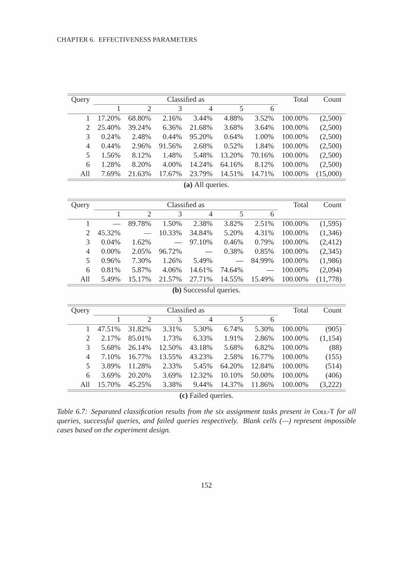
CHAPTER 6. EFFECTIVENESS PARAMETERS
Query Classified as Total Count1 2 3 4 5 6
1 17.20% 68.80% 2.16% 3.44% 4.88% 3.52% 100.00% (2,500)2 25.40% 39.24% 6.36% 21.68% 3.68% 3.64% 100.00% (2,500)3 0.24% 2.48% 0.44% 95.20% 0.64% 1.00% 100.00% (2,500)4 0.44% 2.96% 91.56% 2.68% 0.52% 1.84% 100.00% (2,500)5 1.56% 8.12% 1.48% 5.48% 13.20% 70.16% 100.00% (2,500)6 1.28% 8.20% 4.00% 14.24% 64.16% 8.12% 100.00% (2,500)
All 7.69% 21.63% 17.67% 23.79% 14.51% 14.71% 100.00% (15,000)
(a) All queries.
Query Classified as Total Count1 2 3 4 5 6
1 — 89.78% 1.50% 2.38% 3.82% 2.51% 100.00% (1,595)2 45.32% — 10.33% 34.84% 5.20% 4.31% 100.00% (1,346)3 0.04% 1.62% — 97.10% 0.46% 0.79% 100.00% (2,412)4 0.00% 2.05% 96.72% — 0.38% 0.85% 100.00% (2,345)5 0.96% 7.30% 1.26% 5.49% — 84.99% 100.00% (1,986)6 0.81% 5.87% 4.06% 14.61% 74.64% — 100.00% (2,094)
All 5.49% 15.17% 21.57% 27.71% 14.55% 15.49% 100.00% (11,778)
(b) Successful queries.
Query Classified as Total Count1 2 3 4 5 6
1 47.51% 31.82% 3.31% 5.30% 6.74% 5.30% 100.00% (905)2 2.17% 85.01% 1.73% 6.33% 1.91% 2.86% 100.00% (1,154)3 5.68% 26.14% 12.50% 43.18% 5.68% 6.82% 100.00% (88)4 7.10% 16.77% 13.55% 43.23% 2.58% 16.77% 100.00% (155)5 3.89% 11.28% 2.33% 5.45% 64.20% 12.84% 100.00% (514)6 3.69% 20.20% 3.69% 12.32% 10.10% 50.00% 100.00% (406)
All 15.70% 45.25% 3.38% 9.44% 14.37% 11.86% 100.00% (3,222)
(c) Failed queries.
Table 6.7: Separated classification results from the six assignment tasks present inColl-T for allqueries, successful queries, and failed queries respectively. Blank cells (—) represent impossiblecases based on the experiment design.
152
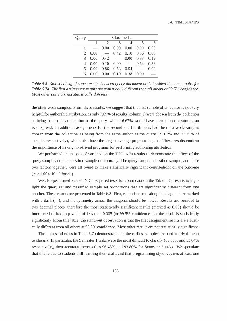
6.4. TIMESTAMPS
Query Classified as1 2 3 4 5 6
1 — 0.00 0.00 0.00 0.00 0.002 0.00 — 0.42 0.10 0.86 0.003 0.00 0.42 — 0.00 0.53 0.194 0.00 0.10 0.00 — 0.54 0.385 0.00 0.86 0.53 0.54 — 0.006 0.00 0.00 0.19 0.38 0.00 —
Table 6.8: Statistical significance results between query-document and classified-document pairs forTable 6.7a. The first assignment results are statistically different than all others at 99.5% confidence.Most other pairs are not statistically different.
the other work samples. From these results, we suggest that the first sample of an author is not very
helpful for authorship attribution, as only 7.69% of results (column 1) werechosen from the collection
as being from the same author as the query, when 16.67% would have beenchosen assuming an
even spread. In addition, assignments for the second and fourth tasks had the most work samples
chosen from the collection as being from the same author as the query (21.63% and 23.79% of
samples respectively), which also have the largest average program lengths. These results confirm
the importance of having non-trivial programs for performing authorshipattribution.
We performed an analysis of variance on the Table 6.7a results to demonstrate the effect of the
query sample and the classified sample on accuracy. The query sample, classified sample, and these
two factors together, were all found to make statistically significant contributions on the outcome
(p< 1.00×10⁻¹⁵ for all).
We also performed Pearson’s Chi-squared tests for count data on the Table 6.7a results to high-
light the query set and classified sample set proportions that are significantly different from one
another. These results are presented in Table 6.8. First, redundant tests along the diagonal are marked
with a dash (—), and the symmetry across the diagonal should be noted. Results are rounded to
two decimal places, therefore the most statistically significant results (markedas 0.00) should be
interpreted to have a p-value of less than 0.005 (or 99.5% confidence thatthe result is statistically
significant). From this table, the stand-out observation is that the first assignment results are statisti-
cally different from all others at 99.5% confidence. Most other results are notstatistically significant.
The successful cases in Table 6.7b demonstrate that the earliest samples are particularly difficult
to classify. In particular, the Semester 1 tasks were the most difficult to classify (63.80% and 53.84%
respectively), then accuracy increased to 96.48% and 93.80% for Semester 2 tasks. We speculate
that this is due to students still learning their craft, and that programming style requires at least one
153

CHAPTER 6. EFFECTIVENESS PARAMETERS
semester to mature. We also note that six cells are marked blank (—), as successful queries cannot
be classified to the query document itself when omitted from the result lists.
In Table 6.7c, the majority of the failed queries occur along the top-left to bottom-right diagonal
of the confusion matrix, showing that many incorrect matches were attributedto samples by other
authors for the same task. This anomaly suggests a number of possibilities. First, there could be
some plagiarism in our collection. Second, there is likely to be some boiler-plate content that is being
picked up in the similarity measurements. Finally, topic influence is also a likely cause. We suspect
that some combination of each of these three factors are contributing to this result, but we cannot
comment further given the ethical and logistical requirements that restrict us from obtaining data that
would allow us to investigate further.
Considering Table 6.7b again, we observe more evidence to suggest thattopic influence con-
tributes towards authorship classification. For all three topics, the majority ofcorrect classifications
arise from matches in the other task of the same semester for every task, except for the second task
of the first semester. In this case, it is most difficult to obtain correct classifications against the first
task since this represents the least mature work sample.
The results in Table 6.7 demonstrate that matches after the timestamp of the query are quite ac-
curate; that is, the “futuristic” or “clairvoyant” matches. For example, the first tasks for Semester 2
and Semester 3 courses demonstrated 96.48% and 79.44% classification accuracy, which is largely
credited to futuristic matches against the second task for those semesters. In practice however, per-
forming futuristic matching may be impractical. For example, allowing new work samples to build
up for a retrospective academic misconduct investigation might only be usedin the most serious of
circumstances, as the individuals concerned would find it difficult to defend themselves based upon
events long past. For example, at RMIT University the head of school must determine if a formal
hearing is to take place within thirty days of being notified of suspected plagiarism, or the case will
lapse [RMIT University, 2002]. Therefore many types of practical authorship investigations may
only consider previous samples of work. As mentioned earlier, the baselinesource code authorship
attribution solutions that we have previously compared our work against in Section 4.5 (p. 106) do
not consider futuristic matches, therefore we explore this area next.
6.5 Using Timestamps to Explore Topical and Temporal Effects
The results from the previous section have made it clear that there are manytopical and temporal
factors that affect classification accuracy. In this section we explore six combinations of these factors:
• Past matches;
154

6.5. USING TIMESTAMPS TO EXPLORE TOPICAL AND TEMPORAL EFFECTS
• Topical effects in isolation;
• Temporal effects in isolation;
• Past matches and current topic matches together;
• Future matches; and
• Future matches and current topic matches together.
By doing this, these experiments allow us to model a real-life authorship attribution scenario by
excluding futuristic matches. This is an experiment that has not been attemptedbefore, as explained
next.
6.5.1 Ignoring Futuristic Matches
The first variation of the Figure 6.5 baseline that we use for exploring the effect of timestamps is to
omit all results that were created after the time period of the query sample. Forexample, Figure 6.6a
shows a scenario where Sample A3 is the query, and all samples for successive tasks are omitted
from consideration. We chose to model this scenario first, as it best represents the real-life scenario
where there is no access to the samples that have not yet been created. This is unlike other authorship
attribution experiments where all samples are simply pooled together for consideration. We would
expect this variation to show that the real-life scenario is more difficult than the baseline experiment,
as all later (and more mature and reliable) samples are omitted.
Results from the Figure 6.6a experiment design are given in Figure 6.6b (dot-dashed line with
diamonds). Overall accuracy dropped to 52.83% from the 78.52% baseline. In particular, queries
for the first task cannot be attributed at all, which accounted for 16.67% of the overall accuracy
drop. Moreover, accuracy for the second task dropped from 53.84% to 38.12%, as these queries had
to exclusively rely on the first assignment, which may often be unreliable forearly career authors.
These results demonstrate a temporal effect, since accuracy is improving rapidly for the first few
tasks.
The varying results for Semester 2 and Semester 3 tasks are of particular interest. Accuracy
dropped by 42.16% and 32.52% for the third to fourth and fifth to sixth tasks respectively compared
to the baseline. However, there was only one fewer success for the fourth task, and accuracy remained
unchanged for the sixth task compared to the baseline. These results demonstrate a topical effect, as
there is a similar pattern for both Semester 2 and Semseter 3.
Having made observations about topical and temporal effects in this experiment, it is of interest
to investigate these separately. We do this next in Sections 6.5.2 and 6.5.3. Moreover, these results
155

CHAPTER 6. EFFECTIVENESS PARAMETERS
show potential for applying source code authorship attribution techniquesin a real-life setting where
future work samples cannot be waited upon, however the accuracy rates clearly need improvement
for the tasks at the beginning of each semester after the first. These improvements are described later
in Section 6.5.4.
Managing the Number of Indexes Again
We also decided to repeat the Figure 6.6 experiment using the index construction method that omits
the ineligible results from the index instead of just the ranked lists as discussed in Section 5.5. This
decision was made as the Figure 6.6 experiment is the first opportunity to compare our index con-
struction methods, where the omission of more than one sample is required.
We found that accuracy dropped by 1.96% from 7,924/15,000 correct classifications (52.83%) to
7,630/15,000 correct classifications (50.87%). The difference was found to be statistically significant
(p = 7.10× 10⁴) using a two-sample test for equality of proportions without continuity correction.
However, we also mention that the effect size is small. The Cohen’sd effect size is 0.04, which is
very small according to the definition by Cohen [1988] whom describedd = 0.2 as small,d = 0.5 as
medium, andd = 0.8 as large. This measurement is important as it isnot affected by sample size,
which contrasts with statistical significance tests [Becker, 2000]. Therefore, we were still able to
discern trends of interest for reporting our timestamp investigation results in this section.
6.5.2 Topical Matches
Much of the discussion in Section 6.4.2 revolved around topical and temporaleffects on authorship
attribution accuracy. So we now begin to explore these separately beginning with topical effects.
Perhaps the best way to explore topical effects is to only allow matches within the same topic. We
essentially have three topics in Coll-T that are three course offerings from three academic semesters.
For example, Figure 6.7a shows a scenario where Sample A3 is the query and all samples from the
third and fourth tasks from the middle semester are the only ones given consideration.
The current topic variation is more effective than the baseline for five of the six data points, as
shown in Figure 6.7b (dashed line with squares), indicating that the topic hasa strong effect on the
ability to attribute authorship. However, accuracy is lower for the second task, as we would expect
matches against the first task to be the most difficult. Overall classification accuracy is 79.59%
compared to 78.52% for the baseline, which was significant (p= 0.02).
156

6.5. USING TIMESTAMPS TO EXPLORE TOPICAL AND TEMPORAL EFFECTS
A1
...... ......
A2
...
A5A3
B5
A6
B2 B3
C1
B1
C3C2 C6C5
J5 J6J2 J3
...
J1
C4
A4
B4
J4
B6
(a)
Assignment Task Number
Acc
urac
y (%
)
1 2 3 4 5 60
10
20
30
40
50
60
70
80
90
100
All Matches (78.52%)Past/Current Assignment Matches (52.83%)
(b)
Figure 6.6: (a) A variation of the Figure 6.4 baseline with samples omitted that were created afterthe time period of the query.(b) Accuracy is stable only for Tasks 4 and 6 compared to the baseline.
157
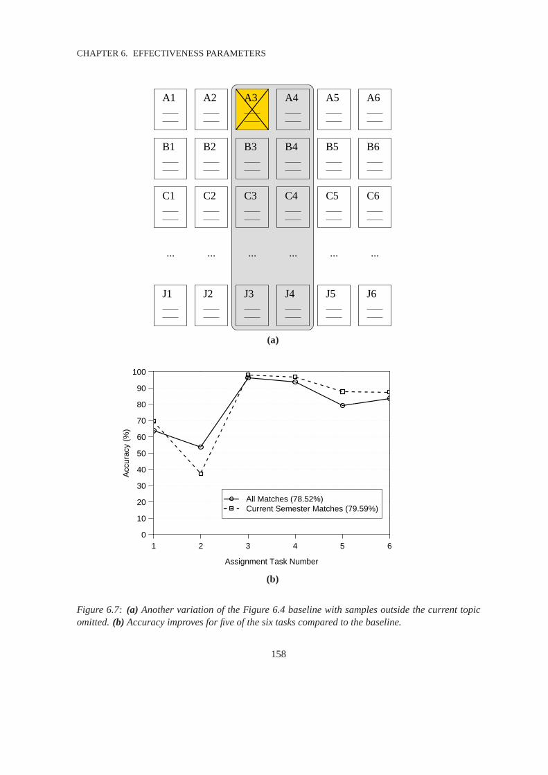
CHAPTER 6. EFFECTIVENESS PARAMETERS
A1
...... ......
A2
...
A5A3
B5
A6
B2 B3
C1
B1
C3C2 C6C5
J5 J6J2 J3
...
J1
C4
A4
B4
J4
B6
(a)
Assignment Task Number
Acc
urac
y (%
)
1 2 3 4 5 60
10
20
30
40
50
60
70
80
90
100
All Matches (78.52%)Current Semester Matches (79.59%)
(b)
Figure 6.7: (a) Another variation of the Figure 6.4 baseline with samples outside the currenttopicomitted.(b) Accuracy improves for five of the six tasks compared to the baseline.
158

6.5. USING TIMESTAMPS TO EXPLORE TOPICAL AND TEMPORAL EFFECTS
6.5.3 Temporal Matches
The inverse of the Section 6.5.2 experiment is required in order to next explore temporal effects.
That is, removing all candidate matches from the current topic will only allow matches from other
semesters. Figure 6.8a demonstrates this for a scenario where Sample A3 is the query, and all samples
from that middle semester are omitted from consideration.
Results for this variation are given in Figure 6.8b (dotted line with triangles). Overall accuracy
dropped to 72.07% from the 78.52% baseline. We note that accuracy for five of the six assignments
is below the baseline, providing further evidence that topic has a strong influence on classification.
However, unlike the baseline and current-topic variants, there is an increase in accuracy from
the first to second and second to third tasks. Little variation exists between theremaining tasks.
As topic influence is removed from this experiment, we can suggest that individual programming
styles improve rapidly across the first semester, resulting in the increasing accuracy we observe up
to the start of the second semester, when style begins to stabilise. Therefore, we speculate that
programming work samples created in the first six months of learning to program are particularly
unreliable as markers of authorial style.
6.5.4 Semester-Based Matches
It is clear that the results obtained from the real-life scenario in Section 6.5.1are quite unsatisfactory,
where only work completed prior to the date of the query was allowed for matching. The baseline is
much better, where all samples are allowed. However, this baseline is impractical for real academic
integrity investigations, as wrongdoing effectively cannot be prosecuted until the end of a program of
study, at which point it is already too late.
A compromise may be to postpone authorship attribution investigations until the endof each
semester. This scenario would additionally make use of all current-topic samples, which we expect
to be strong since topical effects have been shown to be strong in Section 6.5.2. This would allow
misdemeanours to be identified before a student progresses onto followingsubjects. Figure 6.9a
shows the Sample A3 example again, but this time all matches from the middle semester(other than
the query itself) are applicable, unlike the Figure 6.6a scenario.
Results of this variation are plotted in Figure 6.9a (long-dashed line with inverted triangles).
Overall accuracy is 75.31%, which is only 3.21% less than the 78.52% baseline. Most of the dif-
ference is attributed to the second task queries, as they again can only be matched to the first task
samples. Accuracy for these queries dropped to 37.72% from the 53.84%baseline. Therefore we
remark that implementing source code authorship attribution solutions including results up to the end
159

CHAPTER 6. EFFECTIVENESS PARAMETERS
A1
... ...... ...
A2
...
A5 A6A3
B3B2 B5
C1 C2
B1
C5 C6C3
J5J3 J6J1
...
J2
C4
J4
A4
B6B4
(a)
Assignment Task Number
Acc
urac
y (%
)
1 2 3 4 5 60
10
20
30
40
50
60
70
80
90
100
All Matches (78.52%)Current Semester Matches (79.59%)Other Semester Matches (72.07%)
(b)
Figure 6.8: (a) Another variation of the Figure 6.4 baseline with current topic samples omitted. (b)Accuracy improves over the first few time periods, then plateaus out.
160

6.5. USING TIMESTAMPS TO EXPLORE TOPICAL AND TEMPORAL EFFECTS
A1
...... ......
A2
...
A5A3
B5
A6
B2 B3
C1
B1
C3C2 C6C5
J5 J6J2 J3
...
J1
C4
A4
B4
J4
B6
(a)
Assignment Task Number
Acc
urac
y (%
)
1 2 3 4 5 60
10
20
30
40
50
60
70
80
90
100
All Matches (78.52%)Past/Current Assignment Matches (52.83%)Past/Current Semester Matches (75.31%)
(b)
Figure 6.9: (a) Another variation of the Figure 6.4 baseline with future semester results omitted. (b)Baseline accuracy is maintained for most of the tasks.
161

CHAPTER 6. EFFECTIVENESS PARAMETERS
of the university semester is nearly as good as having access to all assignments belonging to each
student at the completion of degrees.
6.5.5 Other Types of Matches
For completeness and curiosity, we provide two more variations of omitting results from the ranked
lists. First, we provide the inverse of the Section 6.5.1 variation that ignored futuristic matches and
instead ignore past matches. An example of this is provided in Figure 6.10a for the Sample A3
example. The other variation is the inverse of the Section 6.5.4 variation that ignored matches from
semesters after the current semester, which now instead ignores matches from semesters before the
current semester. No example is provided for this scenario as it happensto be the same as Figure 6.10a
for Sample A3.
The first variation is provided in Figure 6.10b. The pattern (dotted line with crossed squares) is
largely the inverse of its counterpart as shown, and it is difficult to visually discern the more accurate
result. Accuracy is 55.81%, which is higher than its counterpart (52.83%)but still far behind the
baseline (78.52%). However, this stronger result is further evidence suggesting that maturing of
programming style aids source code authorship attribution effectiveness, since this variation allows
matches to the more mature samples, instead of the less mature samples compared withthe query.
The final variation is provided in Figure 6.11 (dotted line with stars). Accuracy (81.90%) is
higher than both the baseline (78.52%) and the counterpart variation (75.31%). Results for this
variation are more accurate than the baseline for five of the six tasks, providing yet further evidence
that strengthening programming style improves source code authorship attribution accuracy.
In summary, the six variations to the baseline experiment presented in this section have high-
lighted both topical and temporal influences upon accuracy scores that need to be carefully con-
sidered when applying source code authorship attribution to real-life scenarios. In particular, the
Section 6.5.4 variation was found to be highly practical for the real-life academic scenario, whilst
maintaining close accuracy scores to the baseline.
6.6 Using Entropy to Identify Highly Discriminating Features
Sections 6.4 and 6.5 provided a high level analysis showing authorship attribution accuracy across
the six tasks for Coll-T. Between tasks, we would expect the use of many programming constructs to
either increase or decrease depending on the demands of the assessment tasks and growing knowledge
of the individuals. We now provide a feature-level analysis to show how the usage of individual
162

6.6. USING ENTROPY TO IDENTIFY HIGHLY DISCRIMINATING FEATURES
A1
...... ......
A2
...
A5A3
B5
A6
B2 B3
C1
B1
C3C2 C6C5
J5 J6J2 J3
...
J1
C4
A4
B4
J4
B6
(a)
Assignment Task Number
Acc
urac
y (%
)
1 2 3 4 5 60
10
20
30
40
50
60
70
80
90
100
All Matches (78.52%)Past/Current Assignment Matches (52.83%)Current/Future Assignment Matches (55.81%)
(b)
Figure 6.10: (a) Inverse of the Figure 6.6a variation with past matches omitted.(b) Accuracy is2.98% higher overall.
163

CHAPTER 6. EFFECTIVENESS PARAMETERS
Assignment Task Number
Acc
urac
y (%
)
1 2 3 4 5 60
10
20
30
40
50
60
70
80
90
100
All Matches (78.52%)Past/Curr Semester Matches (75.31%)Curr/Future Semester Matches (81.90%)
Figure 6.11: Inverse of the Figure 6.9a variation with matches to past semesters omitted. Accuracyis 6.59% higher overall.
features is evolving in Coll-T, and discuss how this can be applied to improve authorship attribution
accuracy.
In Section 5.3, we investigated how combinations of six classes of features impact the accuracy of
source code authorship attribution tasks. We now examine how these features vary between both indi-
vidual tasks and individual authors. For authorship attribution, we wouldexpect the most remarkable
features to have low between-task dispersion, which whole cohorts use or do not use consistently,
and high between-author dispersion, indicating traits that best identify individual programming pref-
erences. High between-task dispersion would indicate topic influences.
Several options were considered for measuring between-task and between-author dispersion.
Variance and standard deviation were possibilities, but results are cumbersome to compare when
total feature counts vary greatly. We also considered Kolmogorov-Smirnov normality tests, which
generate a value in the range[0,1] indicating how closely the data follows a normal distribution. For
example, skewed data returns a result closer to 0 whilst normally distributed data returns a result
closer to 1. However, there were too many perfect 0 and 1 cases in our data to properly discern
results. We settled on entropy for measuring between-task and between-author dispersion [Shannon,
1948]:
164

6.6. USING ENTROPY TO IDENTIFY HIGHLY DISCRIMINATING FEATURES
Entropy= −s
∑
i=1
pi log2 pi , where (6.1)
• pi is the probability of a symbol occurring, and
• s is the number of symbols.
Entropy is often thought of as a measure of information content. For example, low entropy
indicates that there is little information. In the extreme case of zero entropy, thedata being measured
is entirely predictable, such as the case where every data item is identical. The other extreme is
where all possible occurrences are equally likely. For example, if there are eight possibilities of
equal likelihood, then the entropy value is 3, which is also the number of bits required to store the
information.
In the case of our data, we are measuring the information content for eachspecific feature in
relation to samples from different authors and different tasks — a symbol if the information was to
be coded in binary. If there is a relationship between the occurrence of aprogramming feature and
the author of the program, then there should be low entropy for that feature. If the same feature in
relation to the different programming tasks has a high entropy, then it has little relationship to the
assignment tasks, making it a potentially useful feature for predicting authorship. For our data, the
maximum possible entropy values are− log216 = 2.58 between tasks, and− log2
1272 = 8.09 between
authors. Table 6.9 shows the entropy scores for all features that haveat least fifty instances per sample
on average. The three cases with lowest between-task (“En–Task”) and between-author (“En-Auth”)
entropy values marked in bold are now discussed.
Table 6.9 shows that tabs (‘\t’) and carriage returns (‘\r’) have a high between-task entropy and a
low between-author entropy, indicating their potential for predicting program authorship. Conversely,
the indirect member access (‘->’) and titlecase literalsymbols have low between-task entropy and a
relatively high between-author entropy, making them a better predictor of topic than author.
Concerning the square-bracket token in Table 6.9, the low values were found to be unremarkable
due to a single outlier file that contained 29,232 opening square bracket tokens out of 102,318 tokens
total, which distorted the results. The offending file shown in Figure 6.12 demonstrates a function
that initialises a two-dimensional array using an unnecessary amount of source code, which could be
rewritten using loops. It is hard to explain how this anomalous scenario came tobe. It is plausible that
this code could have been generated by a script. Regardless, it shows avery extreme trait. Perhaps a
more reasonable example concerns a preference where square brackets are not used at all. Figure 6.13
presents a code sample showing how preference towards arrays or pointers respectively could greatly
affect style through the absence of square brackets.
165

CHAPTER 6. EFFECTIVENESS PARAMETERS
Token Count En–Task En–Auth"SPACE" 10,232,897 2.49 7.93"\n" 1,808,827 2.52 8.01Lowercase literal 938,219 2.50 7.99"(" 622,548 2.51 8.01Camelcase literal 504,263 2.48 7.78"\t" 443,138 2.53 6.71"," 335,086 2.46 7.97"=" 270,022 2.52 7.85Other literal 236,174 2.52 7.81"->" 166,478 2.02 7.96"[" 158,671 2.31 7.10"*" 144,188 2.43 7.89Titlecase literal 118,777 2.20 7.86Uppercase literal 114,434 2.42 7.68if 109,837 2.47 8.00int 108,436 2.52 7.93"\r" 102,873 2.50 5.92"." 84,297 2.44 7.70Maximum 2.58 8.09
Table 6.9: Entropy of feature distribution for the six tasks (En–Task) and the272 authors (En–Auth)for all features averaging at least fifty instances per sample inColl-T. Lower entropy values indicatelarger variation (dispersion) within task or author groups. Bold cases are discussed in the text.
166

6.6. USING ENTROPY TO IDENTIFY HIGHLY DISCRIMINATING FEATURES
1 void initialiseLookup(int pageArray[256][256])
2 {
3 pageArray[65][98]=0;
4 pageArray[65][99]=1;
5 pageArray[65][100]=1;
6 pageArray[65][101]=2;
7 pageArray[65][102]=2;
8 pageArray[65][103]=3;
9 pageArray[65][104]=3;
10 pageArray[65][105]=3;
...
14610 pageArray[122][113]=250;
14611 pageArray[122][114]=250;
14612 pageArray[122][115]=250;
14613 pageArray[122][116]=250;
14614 pageArray[122][117]=250;
14615 pageArray[122][118]=251;
14616 pageArray[122][119]=251;
14617 pageArray[122][120]=252;
14618 }
Figure 6.12: Part of a remarkable source code file that contained 29,232 opening square brackettokens out of 102,318 tokens total inColl-T. The file contained a single function that initialised alarge two-dimensional array one value at a time.
int i; int* p;
int values[10]; int* values = calloc(10, sizeof(int));
for (i = 0; i < 10; i++) { for (p = values; p < values + 10; p++) {
values[i] = rand(); *p = rand();
} }
Figure 6.13: Equivalent C program code with and without square brackets for a trivial task involvingthe storage of ten random numbers in an array. These examples show how individual preferences canhave a large impact on programming style.
167

CHAPTER 6. EFFECTIVENESS PARAMETERS
Figure 6.14 shows how contrasting between-author entropy scores cameabout for the carriage
return and parenthesis tokens. The parenthesis tokens demonstrate a normal distribution with no
zero-score or high outliers. However, the carriage return tokens demonstrate a skewed distribution
with many zero-score values and a much larger range. Features with a low entropy like the carriage
return feature demonstrate stronger potential as authorship attribution markers.
We believe indentation should be one of the strongest markers of authorship, but this is not ob-
vious from the results in Table 6.9 for the “SPACE” token, as we would expect the between-author
entropy score to be closer to that of the tab (‘\t’) token, given that both tokens are used for indenta-
tion. From these results, we realised that we had not distinguished betweenspaces used to separate
operators and operands (usually a single space), and spaces used for indentation (usually many spaces
at once). Many 6-grams containing spaces only are expected for indentation, and there is no mech-
anism to detect deeper indentation instances. Therefore we explore a refinement in the use of white
space next.
6.7 Improving Accuracy with Highly Discriminating Features
Up to this point, white space has been managed by a single feature, which needs improvement for
capturing indentation information as concluded in the previous section. We now consider forty white
space tokens representing contiguous sequences of one to forty white spaces to better represent deep
levels of indentation. Similar to Table 6.9, in Table 6.10 we show how the entropy of these new
features varies between tasks and authors, for all white space features with at least ten instances per
sample average.
The “SPACE01” token is still most prevalent but has now been reduced to16.38% of its prior
volume. Space tokens in multiples of three come next (“SPACE03”, “SPACE06”, “SPACE09”,
“SPACE12”), indicating the strong preference for code blocks to be indented in multiples of three
spaces. The “SPACE15” and “SPACE18” tokens are not the next mostprevalent, but have the next
highest between-author entropy scores. Of most interest is the drop in between-author entropy scores
for the remaining five white space features (“SPACE02”, “SPACE04”, “SPACE08”, “SPACE07” and
“SPACE05”), indicating a wider spread of scores and good choices for authorship markers. The
“SPACE02” token had the lowest entropy of all, but we found that the sameoutlier sample shown in
Figure 6.12 partly contributed to this score.
When analysing the spread of scores for the “SPACE02” token similar to Figure 6.14, we again
noticed the extreme contribution of the same outlier discussed in Figure 6.12, but in this case the trend
still held after omitting this program, unlike the square-bracket token case demonstrated in Table 6.9.
168
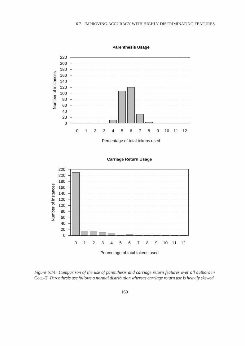
6.7. IMPROVING ACCURACY WITH HIGHLY DISCRIMINATING FEATURES
0 1 2 3 4 5 6 7 8 9 10 11 12
Parenthesis Usage
Percentage of total tokens used
Num
ber
of in
stan
ces
0
20
40
60
80
100
120
140
160
180
200
220
0 1 2 3 4 5 6 7 8 9 10 11 12
Carriage Return Usage
Percentage of total tokens used
Num
ber
of in
stan
ces
0
20
40
60
80
100
120
140
160
180
200
220
Figure 6.14: Comparison of the use of parenthesis and carriage returnfeatures over all authors inColl-T. Parenthesis use follows a normal distribution whereas carriage return use is heavily skewed.
169

CHAPTER 6. EFFECTIVENESS PARAMETERS
Token Count En–Task En–Auth"SPACE01" 1,675,961 2.51 7.98"SPACE03" 366,565 2.50 7.89"SPACE06" 229,320 2.48 7.88"SPACE09" 131,577 2.46 7.76"SPACE12" 88,908 2.47 7.71"SPACE02" 68,845 2.42 6.03"SPACE04" 64,918 2.53 7.05"SPACE15" 47,415 2.46 7.48"SPACE18" 25,261 2.44 7.28"SPACE08" 24,078 2.53 6.65"SPACE07" 22,958 2.49 6.91"SPACE05" 17,344 2.49 6.74Maximum 2.58 8.09
Table 6.10: Entropy of feature distribution for the six tasks (En–Task) and the 272 authors (En–Auth)for white space features with at least ten instances per work sample on average. Smaller entropyvalues indicate larger variation (dispersion) within task and author groups. Bold cases are discussedin the text.
Next we note that we have 2,918 instances of the “SPACE40” token indicating that there may
still be some indentation more than 40 spaces deep, which were treated as a “SPACE40” token plus
another quantity of spaces. However, this amount represents only one totwo instances per sample on
average, so we do not try to introduce more features.
Using the new white space features, we repeated our ten-class authorship attribution experiment
on Coll-T, and found that accuracy jumped from 78.52% (11,700/15,000) to 82.35% (12,352/15,000)
with this feature change alone. We also repeated the experiment on Coll-A and found that accuracy
jumped by a similar margin from 76.78% (12,261/15,969) to 79.66% (12,700/15,943). Both of these
results are statistically significant at the 95% confidence interval using a two-sample test for equality
of proportions with continuity correction (p= 2.20×10⁻¹⁶ andp= 1.50×10⁻¹⁰ respectively). Further
feature refinements like the one presented may yield more effective results, but we would expect
these improvements to be more subtle, as the change made with white space affected the feature
represented by the largest number of tokens in Coll-T. Another reasonable refinement could be to
interpret literals differently to identify authors who use short or long identifier names, but we leave
these refinements for future work.
170

6.8. SUMMARY
6.8 Summary
In this chapter, we explored several factors that affect the accuracy of our approach. These factors
comprised the number of authors, number of samples per author, sample lengths, stylistic strength,
timestamp, and entropy. A key finding is that it takes about one semester for student coding style to
stabilise according to our data, which has implications for practitioners who deal with source code
quality control. The end result for our final model was a statistically significant improvement in
accuracy compared with the version from the previous chapter. Next, in Chapter 7 we compare our
final model to the identified baselines, and investigate improvements to those baselines.
171

CHAPTER 6. EFFECTIVENESS PARAMETERS
172

Chapter 7
Improving Contributions in the Field
The work presented in Chapter 5 introduced our information retrieval approach and the choice of key
parameters including similarity measure, n-gram size, and feature set, usingthe data in Coll-A. Then
in Chapter 6 we explored several factors that affect the accuracy of our approach, including topical
and temporal patterns in the data. The timestamp experiments using Coll-T identified a further
improvement to our feature set involving how white space is used. It remainsto be seen how our
approach performs on a variety of programming languages in a variety of settings, as the experiments
to this point in our approach have used C programming assignments only.
In Section 7.1, we provide accuracy results for our approach on all ofthe collections introduced
in Chapter 3. We then benchmark these against the reimplemented approaches from Section 4.5
(p. 106), to show how much our work has improved the state-of-the-art insource code authorship
attribution accuracy. In Sections 7.2 and 7.3, we next implement some extensions for the previous
approaches that used n-grams and software metrics respectively. Finally, we summarise all of the key
results for this thesis in Section 7.4 before summarising the chapter in Section 7.5.
7.1 Overall Results for the Information Retrieval Approach
When reporting our results for collections Coll-A, Coll-T, Coll-P, and Coll-J, we first reiterate
that a different number of runs is used depending on the collection. For example, in the Section 5.1
(p. 110) methodology based on Coll-A, we described how the experiment is repeated for100 runs,
with each run using a random subset of 10 authors. We have taken carethat roughly the same number
of queries are processed for each collection, however this will never be exact, as the total number of
queries depends upon the authors that are randomly selected for each run. This is as a result of the
number of samples per author greatly varying, as shown in Figure 3.2 (p. 69). The only exception is
173

CHAPTER 7. IMPROVING CONTRIBUTIONS IN THE FIELD
Coll-T, which has exactly six samples for every author. In short, we used 100 runs for Coll-A, 250
runs for Coll-T, 150 runs for Coll-P, and 250 runs for Coll-J.
To enable us to make some generalisations about the differences between our accuracy scores,
we performed a post-hoc analysis to obtain an estimate of the statistical power of these experiments.
Assuming we want high power (0.8, meaning an 80% chance of avoiding a Type 2 error) at 95%
confidence, we have 15,000 queries, and accuracy is 80% for a given method, then our tests are
powerful enough to reject a false null hypothesis for a second method,with a difference in accuracy
of 1.28% or more. We note that this statistical power will remain fairly constant as each experiment
has a similar number of queries.
We report two sets of results in this section concerning the index construction methods reviewed
in this thesis. The first variation was presented in Section 5.1 (p. 110), where the query document
is indexed, but is removed from the results list (presumably the first rank). This variation was used
throughout Chapters 5 and 6 in order to reduce the number of indexes required when developing our
approach.
The second variation from Section 5.5 (p. 132) uses a strict separation of the training and testing
data, where all samples except the query sample are indexed for each run, and each sample is treated
as the query in turn. This variation requires one index per query instead of one index per run, hence
it is much slower. However, since this variation uses astrict leave-one-out cross validation design, it
more closely models the previous work, and is therefore more appropriate for comparison purposes.
The first variation is referred to aslenient leave-one-out(or Lenient), and the second variation is
labelledstrict leave-one-out(or Strict) henceforth. The Lenient approach achieved 80.59% accuracy
for Coll-A, 81.88% for Coll-T, 88.81% for Coll-P, and 81.87% for Coll-J. The Strict approach
achieved 79.70% accuracy for Coll-A, 81.29% for Coll-T, 89.34% for Coll-P, and 80.76% for
Coll-J. These results are summarised in Table 7.1 with the p-values for Z-tests for two proportions.
In absolute values, the Strict variation accuracy results were higher for Coll-P, and the Lenient
variation accuracy results were higher for the other collections. However, considering the p-values
at the 95% confidence level, we note that two of the four differences are statistically insignificant,
and the Coll-A result is borderline (p = 0.05). Therefore we remark that it is satisfactory to use
either of these methods. This finding is consistent with the conclusion in Section5.5 (p. 132) drawn
from Coll-A alone. For the remainder of this chapter, we use the slower Strict variation as it is
more consistent with the previous work reviewed in Section 4.3 (p. 90). TheLenient variation is not
discussed further in this chapter.
Next, it is remarkable to note the higher accuracy obtained for the freelance collections (Strict).
Coll-P accuracy results were around 7% higher than the academic collection accuracy results, and the
174

7.2. IMPROVING N-GRAM APPROACHES
Collection Runs Strict Strict Lenient Lenient p-valueQueries Accuracy Queries Accuracy
Coll-A 100 16,046 79.70% 15,931 80.59% 0.05Coll-T 250 15,000 81.29% 15,000 81.88% 0.19Coll-P 150 16,270 89.34% 16,581 88.81% 0.13Coll-J 250 14,873 80.76% 15,234 81.87% 0.01
Table 7.1: Number of runs and queries to generate results for all four collections.Strict andLenientvariations (discussed in the text) are given with statistical significance results. The accuracy scoresfor the freelance collections are good compared with those in the academic collections consideringthe number of samples per author in each collection.
Coll-J accuracy results were similar to the academic collection accuracy results,but this result was
achieved with the smallest minimum number of training samples per author. Figure 3.3 (p. 71) shows
the actual distributions. We believe the individuals from the freelance collections are motivated to
produce good work for sharing with the Planet Source Code community. Moreover, given that these
authors are not all from a common institution, it is more likely that these authors have more variation
in their coding styles, compared with students from the same institution who may have adopted some
similar traits.
Finally, we extend the Figure 4.4 (p. 107) comparison to also include our results (Strict) in
Figure 7.1. These results show that our accuracy scores are highestexcept when compared to
the Frantzeskou et al. [2006a] baseline for Coll-J. Therefore, our work is state-of-the-art compared
to the previous work, as indicated by the results for three of the four collections.
Having evaluated our work against the previous contributions, we next investigate ways to also
improve the previous contributions starting with Frantzeskou et al. [2006a].
7.2 Improving N-Gram Approaches
Apart from our work, the contribution by Frantzeskou et al. [2006a] isthe only other that uses n-
grams for source code authorship attribution. We leave the n-gram work by Kothari et al. [2007] to
Section 7.3, as the n-gram frequencies used as machine learning features are essentially just another
form of software metric. The core component of the Frantzeskou approach is the production of lists
of unique byte-level n-grams ordered by frequency, and truncated at a fixed profile length. Table 7.2
shows the lengths of the query and author profiles generated using this approach for our collections.
This table first shows the minimum, median, mean, and maximum query lengths for thetest samples.
The same statistics are repeated for the author profiles (or training data), which are generated from
175

CHAPTER 7. IMPROVING CONTRIBUTIONS IN THE FIELD
Burrows a b c d e f g h i j k l
Comparison of Burrows and Baseline Approaches
Burrows and Contributions ‘a’ to ‘l’ (described below)
Acc
urac
y (%
)
0
10
20
30
40
50
60
70
80
90
100
Coll−AColl−TColl−PColl−J
Figure 7.1: Extension of Figure 4.4 (p. 107) showing a comparison of our work (Burrows) to allreimplemented prior contributions:(a) Krsul [1994] (regression analysis and 42 features),(b) Mac-Donell et al. [1999] (k-nearest neighbour and 26 features),(c) MacDonell et al. [1999] (neuralnetwork and 26 features),(d) MacDonell et al. [1999] (regression analysis and 26 features),(e) Dingand Samadzadeh [2004] (regression analysis and 56 features),(f) Frantzeskou et al. [2006a] (simpli-fied profile intersection (L= 2,000) and byte-level 6-grams),(g) Lange and Mancoridis [2007] andcolleagues (nearest neighbour and 56 features),(h) Lange and Mancoridis [2007] and colleagues(Bayesian network and 56 features),(i) Lange and Mancoridis [2007] and colleagues (voting featureintervals and 56 features),(j) Kothari et al. [2007] (Bayesian network and 50 features per author),(k) Kothari et al. [2007] (voting feature intervals and 50 features per author), and(l) Elenbogen andSeliya [2008] (decision tree and 6 features).
176

7.2. IMPROVING N-GRAM APPROACHES
Statistic Coll-A Coll-T Coll-P Coll-JMinimum Query Profile Length 4 345 1 166Median Query Profile Length 2,524 3,050 2,030 1,805Mean Query Profile Length 2,882 3,384 4,162 3,092Maximum Query Profile Length 30,322 22,394 143,223 38,530Minimum Author Profile Length 12,038 7,546 1,335 1,107Median Author Profile Length 22,325 13,376 14,148 8,340Mean Author Profile Length 24,803 13,972 25,805 14,320Maximum Author Profile Length 51,797 38,697 201,334 46,814
Table 7.2: Byte-level n-gram statistics of all four collections comprising the number of unique 6-gramentries in the query profiles and author profiles.
the combined samples of each author. The statistics for the full profiles are reported here, but the
query content is omitted when a query sample belonging to that author is currently in use.
Using these profiles, experiments that follow include the verification of the profile lengthL and
n-gram sizen parameters explored in the Frantzeskou work. Next, we report on the changes in accu-
racy both before and after anonymisation techniques are applied, giventhat different anonymisation
techniques are used for our work and Frantzeskou’s work. Finally, we extend our work with the byte-
level and feature-level n-gram approaches by comparing them both using the Okapi BM25 and SPI
similarity scores used in our work and Frantzeskou’s work respectively.
7.2.1 Profile Length
The profile length parameterL is used in the Frantzeskou approach to denote the length that query
and author profiles are consistently truncated at. This parameter is volatile in that it depends upon
collection sample lengths, as discussed in Section 4.3.4 (p. 94).
The Frantzeskou experiment design simply splits the collections in half into test and training
sets. Therefore the Frantzeskou methodology effectively made classification decisions with only
half-profiles in the previous work. We chose an unequal collection split for our experiment design by
creating author profiles that containall data except for each individual query sample. This approach
maximises the amount of training data available. We believe this experiment designdecision is more
appropriate, as our work in Section 6.1.2 showed that discarding contentresults in severe degradation
of accuracy scores. Moreover, by doing this we have used a leave-one-out cross validation experiment
design, which is consistent with our other experiments.
In Figure 7.2 we present the accuracy scores for a wide range of values ofL from 10≤ L ≤ 56,234
to allow for the length of the longest profile of Coll-A, which is 51,797 byte-level 6-grams. Each
177

CHAPTER 7. IMPROVING CONTRIBUTIONS IN THE FIELD
Frantzeskou Approach Accuracy for Coll−A
Profile Length (L)
Acc
urac
y (%
)
101 101.5 102 102.5 103 103.5 104 104.50
10
20
30
40
50
60
70
80
90
100
Figure 7.2: Classification accuracy of all four collections for Frantzeskou’s profile length L parame-ter using nineteen profile lengths from10≤ L ≤ 56,234.
data point is the mean accuracy score of 100 runs for Coll-A as used in Section 5.1 (p. 110), hence
the plotted line represents approximately 1,900 runs. The n-gram lengthn was kept constant atn= 6,
as this was a common conclusion in an earlier experiment (Section 4.3.4, p. 94).
Accuracy is poorest for the lower values ofL, and accuracy is always increasing withL for
Coll-A. We note that the curve plateaus out for the last few values ofL. This is a result ofL
eventually reaching the longest profile length, thus increasingL after this point does not change the
accuracy scores. This behaviour is expected to occur at a different point for each collection, as the
length of the longest profile differs for each collection (Table 7.2).
Given these results, a suitable modification is to use an infinite profile length anduse the full
set of n-grams as the profile. As an aside, we note that this technique is equivalent toco-ordinate
matching, a ranking technique used in some information retrieval systems [Witten et al., 1999], and
also successfully applied in music information retrieval [Uitdenbogerd and Zobel, 2002]. This is the
approach we adopt in the remainder of this chapter, giving an accuracyusing 6-grams of 75.48% for
178
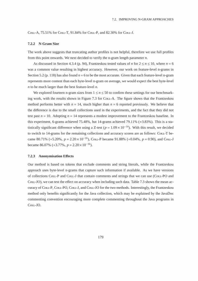
7.2. IMPROVING N-GRAM APPROACHES
Coll-A, 75.51% for Coll-T, 91.84% for Coll-P, and 82.30% for Coll-J.
7.2.2 N-Gram Size
The work above suggests that truncating author profiles is not helpful, therefore we use full profiles
from this point onwards. We next decided to verify the n-gram length parametern.
As discussed in Section 4.3.4 (p. 94), Frantzeskou tested values ofn for 2≤ n≤ 10, wheren= 6
was a common value resulting in highest accuracy. However, our work onfeature-level n-grams in
Section 5.2 (p. 118) has also foundn= 6 to be the most accurate. Given that each feature-level n-gram
represents more content than each byte-level n-gram on average, wewould expect the best byte-level
n to be much larger than the best feature-leveln.
We explored fourteen n-gram sizes from 1≤ n≤ 50 to confirm these settings for our benchmark-
ing work, with the results shown in Figure 7.3 for Coll-A. The figure shows that the Frantzeskou
method performs better withn = 14, much higher thann = 6 reported previously. We believe that
the difference is due to the small collections used in the experiments, and the fact thatthey did not
test pastn= 10. Adoptingn= 14 represents a modest improvement to the Frantzeskou baseline. In
this experiment, 6-grams achieved 75.48%, but 14-grams achieved 79.11%(+3.83%). This is a sta-
tistically significant difference when using a Z-test (p = 1.09×10⁻¹⁴). With this result, we decided
to switch to 14-grams for the remaining collections and accuracy scores areas follows: Coll-T be-
came 80.71% (+5.20%,p= 2.20×10⁻¹⁶), Coll-P became 91.88% (+0.04%,p= 0.90), and Coll-J
became 86.07% (+3.77%,p= 2.20×10⁻¹⁶).
7.2.3 Anonymisation Effects
Our method is based on tokens that exclude comments and string literals, while theFrantzeskou
approach uses byte-level n-grams that capture such information if available. As we have versions
of collections Coll-P and Coll-J that contain comments and strings that we can use (Coll-PO and
Coll-JO), we can test the effect on accuracy when including such data. Table 7.3 shows the mean ac-
curacy of Coll-P, Coll-PO, Coll-J, and Coll-JO for the two methods. Interestingly, the Frantzeskou
method only benefits significantly for the Java collection, which may be explained by the JavaDoc
commenting convention encouraging more complete commenting throughout the Java programs in
Coll-JO.
179
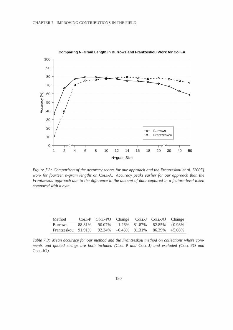
CHAPTER 7. IMPROVING CONTRIBUTIONS IN THE FIELD
Comparing N−Gram Length in Burrows and Frantzeskou Work for Coll−A
N−gram Size
Acc
urac
y (%
)
1 2 4 6 8 10 12 14 16 18 20 30 40 500
10
20
30
40
50
60
70
80
90
100
BurrowsFrantzeskou
Figure 7.3: Comparison of the accuracy scores for our approach andthe Frantzeskou et al. [2005]work for fourteen n-gram lengths onColl-A. Accuracy peaks earlier for our approach than theFrantzeskou approach due to the difference in the amount of data captured in a feature-level tokencompared with a byte.
Method Coll-P Coll-PO Change Coll-J Coll-JO ChangeBurrows 88.81% 90.07% +1.26% 81.87% 82.85%+0.98%Frantzeskou 91.91% 92.34%+0.43% 81.31% 86.39%+5.08%
Table 7.3: Mean accuracy for our method and the Frantzeskou method oncollections where com-ments and quoted strings are both included (Coll-P and Coll-J) and excluded (Coll-PO andColl-JO).
180

7.2. IMPROVING N-GRAM APPROACHES
Byte−Level vs Feature−Level N−Gram Results using Okapi BM25
N−gram Size
Acc
urac
y (%
)
1 2 4 6 8 10 12 14 16 18 20 30 40 500
10
20
30
40
50
60
70
80
90
100
Feature−Level N−gramsByte−Level N−grams
Figure 7.4: Okapi BM25 results using both feature-level n-grams and byte-level n-grams onColl-A.
7.2.4 N-Gram Composition
Results reported in this chapter so far have used feature-level 6-gramsfor our work, and byte-level 14-
grams for the Frantzeskou work. In this section, we examine the effect of swapping the composition
of n-grams for the two methods. That is, we use byte-level n-grams with ourwork, and token-level n-
grams with the Frantzeskou work. To selectn in each case, we repeated the method used to generate
Figure 7.3 on Coll-A. Results are shown in Figure 7.4 for Okapi BM25 and Figure 7.5 for SPI.
The Okapi BM25 similarity scheme achieved highest accuracy of 79.26% when using feature-
level n-grams (n = 6), compared with 76.58% when using byte-level n-grams (n = 18) (2.68% dif-
ference). The SPI similarity scheme achieved highest accuracy of 81.88% when using feature-level
n-grams (n= 10), compared with 79.11% when using byte-level n-grams (n= 14) (2.77% difference).
These comparisons were statistically significant in both cases (p= 8.39×10⁻⁸ andp= 4.55×10⁻¹⁰
respectively).
Using thesen values, we next repeated the experiments on the remaining collections with results
181

CHAPTER 7. IMPROVING CONTRIBUTIONS IN THE FIELD
Byte−Level vs Feature−Level N−Gram Profile Results using SPI
N−gram Size
Acc
urac
y (%
)
1 2 4 6 8 10 12 14 16 18 20 30 40 500
10
20
30
40
50
60
70
80
90
100
Feature−Level N−gram ProfilesByte−Level N−gram Profiles
Figure 7.5: SPI results using both feature-level n-grams and byte-leveln-grams onColl-A.
182

7.3. IMPROVING METRIC-BASED APPROACHES
Okapi BM25 Results SPI ResultsFeature-Level Byte-Level Feature-Level Byte-Level
Collection 6-Grams 18-Grams 10-Grams 14-GramsColl-A 79.70% 76.58% 81.88% 79.11%Coll-T 81.29% 80.80% 80.00% 80.71%Coll-P 89.34% 91.25% 86.83% 91.88%Coll-J 80.76% 86.98% 82.38% 86.07%
Table 7.4: Okapi BM25 results using feature-level 6-grams and byte-level 18-grams, and SPI resultsusing feature-level 10-grams and byte-level 14-grams. The best result for each row depends upon thecollection, making the accuracy of the methods very close.
shown in Table 7.4. Most remarkably, there seems to be little separating the Okapi BM25 and SPI
ranking schemes, and the feature-level and byte-level n-gram methods. To demonstrate this, we
highlighted the best result for each collection in Table 7.4 in bold. SPI with feature-level n-grams was
most accurate for Coll-A, Okapi BM25 with feature-level n-grams was most accurate for Coll-T, SPI
with byte-level n-grams was most accurate for Coll-P, and Okapi BM25 with byte-level n-grams was
most accurate for Coll-J. For now we consider these methods equally effective and discuss possible
future improvements in Chapter 8, but stress that we are using the modifiedL andn parameters to
represent the Frantzeskou work here.
7.3 Improving Metric-Based Approaches
All of the previous approaches to source code authorship attribution thatused software metrics as
features, also used machine learning classifiers in the classification step. In this section, we combine
some of the existing machine learning ideas with one another, and then with our own. We first explore
all untested combinations of feature set and classification algorithm for completeness. Next, we adapt
our own feature set developed in Section 5.3 (p. 122) to the machine learning algorithms used in this
thesis, and then extend this to n-grams of features.
7.3.1 Evaluating Combinations of Metrics and Classifiers
Several combinations of classification algorithm and feature set have been proposed in the literature,
as reviewed in Section 4.3 (p. 90). However, it is not obvious if the appropriate feature sets have been
paired with the appropriate classification algorithms since there are many possible combinations. We
resolve this problem by exploring all possible combinations from the previous work in this section.
183
CHAPTER 7. IMPROVING CONTRIBUTIONS IN THE FIELD
We also introduce a support vector machine (SVM) classifier, as this classifier has been mentioned
many times in the literature for natural language authorship attribution in Section 4.2 (p. 85). Support
vector machines are known to be effective when dealing with large numbers of features [Colas et al.,
2007]. Several implementations of support vector machines are available inWeka, however some
do not handle multi-valued nominal classes, or assume that the input is in a specific format that is
not suitable for our experiments. We used theweka.classifiers.functions.SMOclassifier, which trains
a support vector classifier using the sequential minimal optimisation algorithm [Platt, 1998]. With
the inclusion of the support vector machine with the existing classification algorithms from Table 4.2
(p. 104), we now haveeightclassification algorithms.
Concerning feature sets, we have six feature sets so far as discussedin Section 4.4.2 (p. 102).
One further option is to pool all feature sets (except for Kothari et al. [2007]) into a combined feature
set. We name this setKMDLE in reference to the initials of the five authors. The aim here is to
explore how well the individual contributions work together. Note that we have deliberately omitted
the Kothari et al. [2007] features from the pool, as these features areoptimised for each individual
author, which are not compatible with the methodology for deriving the other sets. Combining the
other 5 feature sets resulted in the new feature set having 168 metrics afterredundancy was removed.
With the inclusion of the combined feature set, we now havesevenfeature sets.
Together, we now havefifty-six (8×7) combinations of classification algorithm and feature set,
and only results for the previously published combinations have been explored and reimplemented
in our experiment in Figure 4.4 (p. 107). Figure 7.6 shows the mean accuracy scores over all four
collections of all combinations of classification algorithm and feature set. Generally, the more metrics
used as features, the better the performance of each classifier. An exception is the MacDonell metric
set (twenty-six metrics), which performed marginally better than the Krsul metric set (forty-two
metrics), however this may be due to the fact that the Krsul [1994] work was the first contribution in
the field.
Figure 7.6 results show that the accuracy for the neural network classifier was highest for six of
the seven metric sets. The only exception was the Elenbogen metric set wherethe nearest neighbour
accuracy score was 0.11% above the neural network accuracy score. However, this high accuracy
comes at a cost. From anecdotal evidence, we simply mention that the neuralnetwork classifier was
the slowest of all, therefore an alternative may be required if speed is important.
Figure 7.6 also shows that the KMDLE and Kothari feature sets almost always have the highest
accuracy scores. Accuracy for the Kothari set was highest for sixof the classifiers, and accuracy for
the KMDLE set was highest for the remaining two classifiers. This result again represents a time
versus accuracy trade-off, as these two sets are the largest.
184

7.3. IMPROVING METRIC-BASED APPROACHES
NeuNt NNei KNNei Regre DecTr SVM Bayes VFI
Average of Coll−A/T/P/J Accuracy for All Feature Sets and Classifiers
Classifier
Acc
urac
y (%
)
0
10
20
30
40
50
60
70
80
90
100
KrsulMacDonellDingLangeElenbogenKMDLEKothari
Figure 7.6: Accuracy scores for the eight classifiers and seven metric sets averaged acrossColl-A,Coll-T, Coll-P, and Coll-J. The classifiers are the neural network (NeuNt), nearest neighbour(NNei), k-nearest neighbour (KNN), regression analysis (Regre), decision tree (DecTr), support vec-tor machine (SVM), Naive Bayes (Bayes), and voting feature interval (VFI) classifiers. The metricsets are named after the respective authors from Table C.1 (p. 221) in Appendix C, with “KMDLE”representing the combined metric set of the first five authors from the appendix. Complete and un-averaged results are given later in Table 7.8 from Section 7.4.
185

CHAPTER 7. IMPROVING CONTRIBUTIONS IN THE FIELD
Classifier NeuNt NNei KNNei Regre DecTr SVM Bayes VFIAccuracy 60.42% 56.37% 34.29% 52.31% 51.15% 53.64% 51.35% 46.91%
Table 7.5: Averaged results from Figure 7.6 for all classification algorithms (neural network, nearestneighbour, k-nearest neighbour, regression analysis, decision tree, support vector machine, NaiveBayes, and voting feature intervals).
Of particular interest is the result ordering of accuracy for the seven metric sets for each clas-
sification algorithm, which vary little. These results demonstrate the importance ofchoosing an
appropriate set of features regardless of the classification algorithm in use. Moreover, the order gen-
erally follows the chronological order of the contributions. The only exceptions are the Elenbogen
metrics that have the lowest accuracy scores for all classifiers and the support vector machine results
mentioned already. That is, the Krsul [1994] results are poorer than theMacDonell et al. [1999]
results, which in turn are poorer than the Ding and Samadzadeh [2004] results, which are poorer than
the Lange and Mancoridis [2007] results, which are poorer than the Kothari et al. [2007] and KM-
DLE results. The results generally demonstrate a gradual increase in the accuracy scores since 1994,
which is encouraging.
Next, we note that there are a few common themes from Appendix C, which could impact the ac-
curacy scores for the individual metrics sets. First, there are some features that are language specific.
For example, the object-oriented metrics are less likely to be effective for the C-based collections
(Coll-A and Coll-T). We do not attempt to address this shortcoming as we wish to reimplement the
metric sets as closely as possible. However, the contributions that used more language independent
metrics (such as those that deal with white space usage, for example), should provide more consistent
accuracy scores.
We also anticipate some poorer results for the metric sets with larger proportions of metrics
based on comments for our collections. This is a result of anonymising Coll-A, Coll-T, Coll-P, and
Coll-J, which resulted in no comments remaining in the code.
In Tables 7.5 and 7.6, we average the results from Figure 7.6 over all classifiers and metric sets
respectively. Overall, the Kothari feature set is the most accurate, andthe neural network is the most
accurate classifier. The support vector machine was a close second throughout our study, however the
aggregation of results pushes the SVM down to third, as there were some poor results for the metric
sets with only a small number of metrics. We remark that SVMs should be avoidedfor small feature
sets.
186

7.3. IMPROVING METRIC-BASED APPROACHES
Feature Set Krsul MacD Ding Lange Elenb KMDLE KothariAccuracy 49.09% 49.33% 57.43% 59.50% 28.28% 64.55% 67.21%
Table 7.6: Averaged results from Figure 7.6 for all feature sets (Krsul, MacDonell, Ding, Lange,Elenbogen, KMDLE, and Kothari).
Property Coll-A Coll-T Coll-P Coll-PO Coll-J Coll-JO(a) Total 6-grams 5,700,748 8,073,427 6,388,394 9,594,049 1,909,534 2,564,762(b) Unique 6-grams 454,378 622,112 387,227 490,761 110,893 151,587(c) (a)/(b) 12.55 12.98 16.50 19.55 17.22 16.92
Table 7.7: Key collection properties for all collections concerning feature-level 6-grams extractedwith our approach. The total number of 6-grams, number of unique 6-grams, and the ratio betweenthese are shown.
7.3.2 Machine Learning with N-Gram Features
In Section 7.2.4, we recommended either 6-grams of tokens or 14-grams of bytes as features when
using information retrieval techniques for matching. However, the featurespace of n-grams this size
would be too large for most machine learning classifiers to handle. Table 7.7 shows that there are
over 100,000 distinct feature-level 6-grams in each of the collections. Hence we use unigrams as
features and explore the performance of the classifiers from the previous section. As a first step
using the operator, keyword, and white space features, as selected in Sections 5.3 and 6.7, we end
up with 114 C features, 148 C/C++ features, and 132 Java features. These features are based upon
operator and keyword charts from programming text books and international standards as summarised
in Tables D.1, D.2, and D.3 in Appendix D. The feature counts for each sample are normalised against
the average number of tokens in the sample and rounded to the nearest integer.
Figure 7.7 gives the accuracy scores for all eight of the tested classifiers for each of the four col-
lections. The support vector machine gave the most accurate result of allcollections with 80.37% for
Coll-P. The neural network classifier was second with 79.90% (p= 0.28). However, the neural net-
work classifier was more accurate than the support vector machine for thethree remaining collections:
Coll-A was 65.46% (+1.61%,p= 2.58×10⁻³), Coll-T was 59.11% (+1.94%,p= 6.89×10⁻⁴), and
Coll-J was 71.28% (+0.66%,p= 0.22). Two of the differences are statistically significant in favour
of the neural network classifier at 95% confidence using a Z-test.
The least accurate algorithm was the k-nearest neighbour classifier, thus we extended our work
for values ofk other thank= 20 (k ∈ {1,2,3,4,5,10,20,30}). We found that accuracy degraded for all
successive values ofk, so we remark that the k-nearest neighbour classifier is inferior to the nearest
187

CHAPTER 7. IMPROVING CONTRIBUTIONS IN THE FIELD
NeuNt NNei KNNei Regre DecTr SVM Bayes VFI
Comparison of Eight Weka Classifiers with Normalised Token Count Features
Classifier
Acc
urac
y (%
)
0
10
20
30
40
50
60
70
80
90
100
Coll−AColl−TColl−PColl−J
Figure 7.7: Comparison of eight Weka classifiers (neural network, nearest neighbour, k-nearestneighbour, regression analysis, decision tree, support vector machine, Naive Bayes, and voting fea-ture intervals) using unigram tokens as features, leave-one-out crossvalidation, and default param-eters in Weka except for the k-nearest neighbour classifier where K=20 was used.
188

7.4. SUMMARY OF RESULTS
neighbour classifier for our problem domain.
A comparison can be made on these results using normalised counts of unigrams as features,
compared with the unigram results for our approach and the Frantzeskouapproach previously given
in Figure 7.3 — 36.37% for our approach and 11.34% for Frantzeskou. These results are clearly
inferior to the accuracy achieved using the machine learning classifiers, however it is also obvious
that our work and the Frantzeskou work is not intended to be effective on unigrams. This is explored
in our next experiment using n-gram based metrics other than unigrams.
First, increasingn creates a problem in that it leads to an exponential increase in the number of
features. Therefore, to test larger values ofn with the machine classifiers, we chose to truncate the
feature space, and only use the most commonly occurring n-grams based on collection-wide statistics.
Figure 7.8 provides the accuracy scores for 6-gram representationswith the number of features cut-
off at 9 different points from 10 to 1,000 features for Coll-A. The leading neural network and support
vector machine classifiers are shown only for brevity. The results using unigrams from Figure 7.7
are shown as the baseline at the far right of the graph for each method for comparison. These results
demonstrate that classification accuracy generally increases as more 6-gram features are included.
This trend is particularly strong for the support vector machine classifier,which is also the weakest
for the smallest feature sets. Interestingly, these results show that it only takes around 56 n-gram
features to meet the unigram baseline for each classifier, and results generally continue to improve
further up to the final data point at 1,000 features.
These results can motivate new research using n-gram features combined with classifiers. How-
ever, this type of experiment does not scale well, and a high performancecomputing cluster was
needed to produce the results for the 178 to 1,000 feature data points for some of the classification
algorithms. Future work is needed to identify classifiers with the best compromise between time
requirements and accuracy. One option is to explore other implementations of neural networks and
support vector machines in Weka.
7.4 Summary of Results
Figure 7.9 gives the accuracy scores for the leading approaches forall four collections. That is, our
approach, the Frantzeskou approach with modified parameters, and the neural network coupled with
the Kothari and KMDLE feature sets. Accuracy scores for the machine learning approaches trail the
other approaches for all collections except for the neural network withthe Kothari feature set, which
is 2.83% higher than our work for Coll-J only. Using selected n-grams as features for the machine
learning classifiers showed promise in Section 7.3.2, however scalability problems remain.
189

CHAPTER 7. IMPROVING CONTRIBUTIONS IN THE FIELD
Machine Learning Results with 6−Gram and Unigram Features
Number of 6−Gram Features and Unigram Baseline
Acc
urac
y (%
)
10 18 32 56 100 178 316 562 1000 baseline0
10
20
30
40
50
60
70
80
90
100
Neural NetworkSupport Vector Machine
Figure 7.8: Comparison of the neural network and support vector machine algorithms using 10to 1,000 of the most common n-gram features (in logarithmic increments) against the baseline fromFigure 7.7 (rightmost data point) using only unigrams. Results are forColl-A only, and the otherclassifiers are omitted for brevity.
190
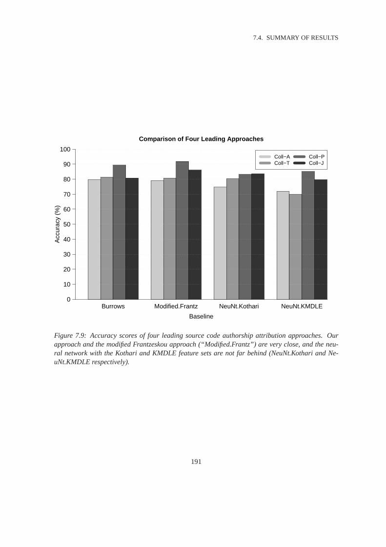
7.4. SUMMARY OF RESULTS
Burrows Modified.Frantz NeuNt.Kothari NeuNt.KMDLE
Comparison of Four Leading Approaches
Baseline
Acc
urac
y (%
)
0
10
20
30
40
50
60
70
80
90
100Coll−AColl−T
Coll−PColl−J
Figure 7.9: Accuracy scores of four leading source code authorship attribution approaches. Ourapproach and the modified Frantzeskou approach (“Modified.Frantz”) are very close, and the neu-ral network with the Kothari and KMDLE feature sets are not far behind (NeuNt.Kothari and Ne-uNt.KMDLE respectively).
191

CHAPTER 7. IMPROVING CONTRIBUTIONS IN THE FIELD
The accuracy scores for our approach and the modified Frantzeskouapproach are close. The
reported results for our method are for 6-grams with the Okapi BM25 similaritymeasure using op-
erators, keywords, and white space tokens as features. The Frantzeskou results are for 14-grams of
bytes without using the profile lengthL parameter. Our approach was more accurate than the mod-
ified Frantzeskou approach for Coll-A with 79.70% accuracy (+0.59%), and Coll-T with 81.29%
accuracy (+0.58%). The modified Frantzeskou approach was more accurate for Coll-P with 91.91%
accuracy (+2.54%) and Coll-J with 86.07% accuracy (+5.31%). In short, our approach was more
accurate for the academic collections, and the modified Frantzeskou approach was more accurate for
the freelance collections.
The properties of the academic collections compared to the freelance collections may contribute
to the differing results between the types of collections. In particular, Table 3.2 (p. 69) shows that
the median lines of code for the freelance samples is less than half that of the academic samples.
Future work using our approach could attempt to bridge or further explainthis gap by exploring
several choices for the document length weighting parameter other than thedefaultb= 0.75. Addi-
tionally, other similarity metrics in Zettair that do not have inbuilt document length weighting (such
as Cosine), could be explored to determine whether document length weighting in our work is over-
compensated. Finally, we could experiment with subsets of our collections, such that the collection
properties between the academic and freelance collections become closer.
Table 7.8 gives accuracy scores for all of the methods executed on ourcollections as a reference
to other researchers and for benchmarking any future techniques. Toour knowledge, this is the
first ever attempt to test all existing source code attribution techniques on thesame collections. The
top-left portion of the table gives results for all combinations of Okapi BM25 and SPI similarity
measures, and feature-level and byte-level n-grams for the similarity measurement methods as given
in Table 7.4. The bottom-right portion of the table gives results for all combinations of the classifiers
and metric sets in the literature, including the SVM classifier and KMDLE metric setfor the machine
learning methods as given in Figure 7.6.
The top-right portion of Table 7.8 uses normalised counts of n-gram occurrences as features.
Some results from Figure 7.8 for 1,000 6-gram token-level features areincluded in italics. As dis-
cussed in Section 7.3.2, the number of features to process increases exponentially for n-grams of
features. Given this, it becomes necessary to truncate the feature space and only use the most com-
monly occurring n-grams. We found that our use of the Weka framework did not scale to a suitably
large number of features to find the most effective number of features. Accuracy scores were still in-
creasing at 1,000 features for most classification algorithms, which was thelargest amount we could
test on the high-performance computing cluster. When a suitable alternativeis found to process the
192

7.4. SUMMARY OF RESULTS
Feature Collection Ranking Method ClassifierSet Okapi SPI NeuNt NNei KNNei Regre DecTr SVM Bayes VFIBurrows Coll-A 79.70 81.88 76.46 66.08 37.01 60.54 56.61 77.23 73.24 56.44Feature Coll-T 81.29 80.006-grams Coll-P 89.34 86.83(Okapi), Coll-PO 90.07 86.9310-grams Coll-J 80.76 82.38(SPI) Coll-JO 82.85 83.21Frantzeskou Coll-A 76.58 79.11Byte Coll-T 80.80 80.7118-grams Coll-P 91.25 91.88(Okapi), Coll-PO 92.65 93.8614-grams Coll-J 86.98 86.07(SPI) Coll-JO 89.03 88.3642 Coll-A 54.48 46.98 27.71 48.68 44.25 45.82 45.40 41.96Krsul Coll-T 42.79 32.71 13.85 35.38 34.33 37.41 35.55 30.87Metrics Coll-P 69.65 65.69 50.05 62.34 59.21 69.17 62.88 54.79
Coll-PO 71.71 65.66 50.88 63.35 59.91 70.88 65.71 55.77Coll-J 64.84 58.83 37.06 57.13 58.17 61.69 59.21 52.81Coll-JO 69.31 62.52 38.46 61.09 61.16 66.51 62.45 57.06
26 Coll-A 54.74 52.57 36.77 48.35 44.29 39.86 43.41 42.78MacDonell Coll-T 48.93 42.11 16.41 40.95 38.69 25.43 39.67 36.49Metrics Coll-P 69.53 66.55 47.41 63.32 60.44 59.12 64.44 56.53
Coll-PO 72.10 69.41 48.85 64.99 60.24 65.34 68.02 59.37Coll-J 64.68 63.31 37.69 57.52 55.82 49.33 58.78 55.52Coll-JO 69.51 67.32 39.60 60.63 59.61 55.59 62.12 59.68
56 Coll-A 65.88 62.07 39.35 56.76 52.94 53.97 51.78 49.32Ding Coll-T 59.10 55.59 20.68 46.17 46.29 50.56 48.79 40.13Metrics Coll-P 74.37 71.28 49.93 67.02 64.52 72.92 67.52 61.02
Coll-PO 76.79 72.06 51.89 68.69 64.18 76.03 68.72 63.68Coll-J 71.66 67.25 37.71 60.49 63.74 68.13 62.85 57.65Coll-JO 74.83 70.67 39.75 63.74 66.17 73.28 64.05 60.66
52 Coll-A 64.83 62.56 40.15 58.03 55.84 59.83 51.46 51.54Lange Coll-T 60.53 54.47 19.07 45.84 47.88 55.00 52.14 42.93Metrics Coll-P 76.88 73.11 52.45 67.00 64.66 77.26 66.13 63.01
Coll-PO 79.77 76.55 53.22 69.28 64.79 80.31 69.52 64.75Coll-J 76.04 74.88 37.83 63.43 64.11 76.26 63.71 59.74Coll-JO 79.48 78.01 39.93 66.00 66.16 79.37 66.56 63.72
6 Coll-A 25.41 28.09 18.62 24.23 24.02 13.67 19.21 21.15Elenbogen Coll-T 12.93 12.03 7.31 13.44 12.65 1.08 12.69 13.47Metrics Coll-P 41.58 40.29 34.03 41.47 40.85 31.69 35.25 30.47
Coll-PO 44.08 43.24 36.12 46.32 44.69 35.34 38.12 33.30Coll-J 46.03 46.00 33.39 46.39 46.57 36.95 42.78 40.08Coll-JO 47.75 45.14 32.16 48.77 48.17 36.52 42.96 42.17
168 Coll-A 72.37 62.47 44.15 63.40 59.99 70.81 58.89 54.50KMDLE Coll-T 69.63 57.78 21.92 50.55 52.25 67.96 54.67 44.82Metrics Coll-P 84.09 80.15 57.30 72.10 69.45 84.75 70.95 64.72
Coll-PO 85.84 81.81 58.03 70.84 68.78 86.18 72.70 65.65Coll-J 79.02 76.08 42.14 65.33 66.58 78.76 64.70 59.48Coll-JO 81.74 78.14 41.99 66.00 66.20 80.86 67.53 60.85
50 Coll-A 74.71 63.62 48.26 63.37 53.41 68.67 63.34 51.21Kothari Coll-T 80.37 65.55 31.43 60.46 55.75 73.63 61.64 47.63Metrics Coll-P 83.19 74.79 57.63 73.67 68.17 77.89 71.46 63.41(per Coll-PO 84.60 75.56 60.32 75.51 68.80 79.85 71.92 65.34author) Coll-J 83.59 77.70 48.28 74.78 72.66 81.37 65.95 54.09
Coll-JO 83.86 78.22 49.26 76.75 74.70 82.57 67.45 53.67
Table 7.8: Summary scores for our work, baselines, and other variations from this chapter. Someresults from Figure 7.8 for 1,000 6-grams are also given in the top-right section in italics. Note thathaving values in the bottom-left section would be nonsensical as discussedin the text.
193
CHAPTER 7. IMPROVING CONTRIBUTIONS IN THE FIELD
large number of features required, follow-up experiments are needed toverify if n = 6 is the most
suitable value for this problem.
The bottom-left portion of the Table 7.8 remains blank since no one has yet applied information
retrieval style ranking to sets of metric measurements. It is not obvious how (or even why) one would
implement this.
Some curious outlier results are present in Table 7.8. For example, the result for the SVM clas-
sifier and the Elenbogen feature set for Coll-T shows just 1.08% accuracy, which is well below
the 10% random chance threshold. The remaining results for the Elenbogen feature set are around
random chance for Coll-T, being between 7.31% and 13.47%. Moreover, Coll-A results are not
much higher with scores between 13.67% and 28.09%. We do not believe these poor accuracy results
are collection-specific, as the result trends for all collections on all metric-based results are almost al-
ways the same: Coll-T results are the lowest, Coll-A results are the second lowest, and the freelance
collections results are the highest. The only exception is the Naive Bayes classifier for the Lange
metrics for Coll-A and Coll-T. The remaining considerations are the choice of metric set and clas-
sifier. Concerning the metrics, it is clear that the Elenbogen metrics have the lowest accuracy scores
in general, but this does not explain why the 1.08% result is so far below random chance. We would
expect a poor choice of metrics to provide around 10% accuracy if they were not more helpful than
guesswork. So we expect that there is some anomalous behaviour in the classifier. We have already
shown in Figure 7.8 that the support vector machine is poor for low numbersof features. We remark
that one of the six Elenbogen features is completely useless for the (anonymised) Coll-T collection
(Appendix C – E02: “number of comments”). Therefore, we suggest that the combination of a low
number of features and having a completely redundant feature is causinganomalous behaviour in the
support vector machine, and almost always incorrect results.
Finally, we remark that Table 7.8 represents the largest empirical contribution on source code
authorship attribution to the best of our knowledge. Assuming 15,000 queries per measurement are
reported, and with 368 measurements, this represents around 5,520,000 queries in total. These results
provide a clear set of benchmarks for further advancing the field. Moreover, the purpose of this table
is to make clear what has and has not been done in the field of source codeauthorship attribution for
future advancement of the field. By presenting all combinations of the previous work, the table also
discourages frivolous pairings of just another classifier with just another metric set, which should
encourage more work on the n-gram approaches in the future. These are the results that are leading
the field.
194

7.5. SUMMARY
7.5 Summary
In addition to our information retrieval contribution to source code authorship attribution, at least
eight other research groups have published in this area, but relative accuracy was unclear given
varying collections and evaluation methodologies. This chapter has brought all the previous work
together for a comprehensive comparison. The results suggested that our work and our extension of
Frantzeskou’s work are leading the field. Next, in Chapter 8 we summarise the findings in this thesis
and outline areas for future work.
195

CHAPTER 7. IMPROVING CONTRIBUTIONS IN THE FIELD
196
Chapter 8
Conclusions
Authorship attribution is the process of assigning samples of work to their authors based on style
traits in training data. This problem has been extensively studied in relation to natural language, but
is far less developed in relation to source code. The source code authorship attribution contributions
of this thesis fall within five themes, and we now summarise the key results and their significance in
turn, followed by future work and a summary.
8.1 Collections
The collections used in the research described in this thesis were designedto be large enough such that
we did not need to use any whole collection at once. Instead, we were ableto randomly sample parts
of the whole collections to form many runs, which allowed us to perform many more classifications
than in the previous work. The importance of this methodology is that we had sufficient queries for
statistical significance tests, which was lacking in previous work, due to the modest collection sizes
used.
In developing our collections and reviewing the collections in previous work, we developed a list
of eleven properties for effective use of authorship attribution collections. We demonstrated that we
have met these properties for our collections, with the exceptions of not being about to guarantee
that authorship is always correct and never shared due to plagiarism and similar problems. The
consequence is that imperfect ground truth may reduce the accuracy obtainable, therefore our results
should be considered slightly conservative, compared with collections where ground truth is known
to be perfect. The eleven properties can also act as a checklist for the benefit of other researchers,
and we recommend its use for future collection construction.
The remaining contribution concerning collections is availability. We have released statistics
197

CHAPTER 8. CONCLUSIONS
about token frequencies in the collections, which does not have intellectual property problems, unlike
any release of the original collections. These statistics are suitable for measuring the frequency of
tokens that can be used to reimplement many of the software metrics reviewed inthis thesis. We also
provided a full explanation for reproducing the freelance collections based upon the original online
source data.
8.2 Benchmarking Previous Contributions
The review of previous contributions began with plagiarism detection and genre classification, as
these areas are closely related to those of previous work. The common methodologies used in au-
thorship attribution were highlighted. We next described the similarities and differences between
authorship attribution for natural language and source code. The choice of features for natural lan-
guage authorship attribution is obviously different, but several of the classification algorithms are
shared.
The review of the previous work in the field of source code authorship attribution identified
eight contributions. It was clear that there was little agreement between keychoices of feature set,
classifier, and similarity metric, and the lack of agreement was exacerbated by the few benchmarking
experiments.
Given the above shortcomings, our first experiment was to reimplement andcompare the eight
contributions using our collections. Our results suggested that the Frantzeskou approach [Frantzeskou
et al., 2006a] using the simplified profile intersection similarity measure on authorprofiles of byte-
level n-grams, is more effective than the machine learning and software metric contributions. The
results also provided a comprehensive set of benchmark scores for comparison with our own infor-
mation retrieval contribution. This contribution is significant, as it is the first full evaluation of all
published source code authorship attribution contributions.
8.3 Applying Information Retrieval
The review of previous contributions made it clear that the use of n-grams and similarity measures,
such as coordinate matching, was underexplored for source code authorship attribution. We proposed
an information retrieval approach motivated by the previous source codeplagiarism detection work
of Burrows et al. [2006].
From the initial experiments using an information retrieval approach, we identified an appropriate
n-gram length, similarity measure, and feature set. Results for the choice ofn-gram length showed
that n = 6 is suitable. Concerning the similarity measure, Okapi BM25 was shown to be more ef-
198
8.4. EFFECTIVENESS PARAMETERS
fective than cosine, pivoted cosine, language modelling with Dirichlet smoothing, and Author1 that
we developed ourselves. Six feature classes were evaluated consistingof operators, keywords, white
space tokens, literal tokens, input/output tokens, and function tokens. The combination of opera-
tors, keywords, and white space tokens, was identified as being highly effective. These experiments
used mean reciprocal rank and mean average precision information retrieval evaluation measures, to
quantify the quality of the ranked lists returned by the search engine.
When investigating the method for making authorship decisions, we found thatusing the author
of the top ranked sample was more effective than using ranked lists as a whole, whether using the
positions in the ranked lists (average precision), or normalised weights. This result suggests that some
samples may be less helpful markers of authorship than others, since all but one result was discarded
for each decision.
Omitting the query sample from the index results in a very large increase in running time, as a new
index is needed for each successive query to ensure there is no bias when comparing techniques. We
investigated leaving the query sample in the index, and instead omitting it from the returned ranked
lists of results. This has the benefit of reducing the number of indexes from one per query to one per
run. While this variation affects the term data in the index, we showed that the difference in results
between this faster design and the alternative is statistically insignificant, and hence acceptable.
The conclusion in Chapter 5 is the comparison of our initial model to the benchmarks evaluated
in Chapter 4. The initial results using Coll-A already indicated that our work performs better than
previously published methods at this point.
8.4 Effectiveness Parameters
When developing the initial model described above, some other key factorshad to be kept constant,
such as the number of authors and number of samples per author. We found that there is no bench-
mark for these factors for source code authorship attribution, but we were able to demonstrate the
good scalability of our approach in terms of number of authors compared witha natural language
authorship attribution benchmark.
We next explored the effect of sample size, and showed that our model performed similarly on
short and long query samples. We also explored the stylistic strength of the samples as measured with
criteria common to computer science assessment, and found that a correlationdoes not exist between
stylistic strength and authorship attribution accuracy. This implies that samples with both good and
poor quality coding styles can be attributed with similar levels of accuracy.
An important contribution in Chapter 6 concerned sample timestamp as a confound. We inves-
199
CHAPTER 8. CONCLUSIONS
tigated topical and temporal effects in turn and showed that both strongly affect accuracy. That is,
accuracy increases if there is topical data available, and accuracy is higher for later query samples
than earlier ones.
We also demonstrated that accuracy scores for typical authorship attribution experiments and
the real-life scenario of attributing authorship of student programs in educational institutions differ
greatly. In the real-life scenario, samples dated after the query sample obviously do not yet exist,
and should therefore be discounted from training. We found that the greatly reduced accuracy scores
were unacceptable for the real-life scenario. However, we found thatallowing all matches from the
current semester in addition to the previous samples is nearly as effective as allowing the full set.
The key finding from the timestamp investigation is that accuracy scores plateaued roughly from
the third task of six when exploring timestamps in isolation. We suggest this indicates the amount of
time for coding style to stabilise. This finding has implications for those developingcoding standards,
and monitoring compliance within organisations.
We concluded Chapter 6 by investigating how the use of individual features changes between
individual authors and tasks using entropy. We found that capturing white space in blocks was more
effective than processing spaces individually.
8.5 Improving Contributions in the Field
The previous work in source code authorship attribution lacked a benchmarking study to bring all the
work in the field together for an overall comparison, which was a problem we have now addressed.
We also implemented some obvious variations of the previous work, such as exchanging the types of
n-grams used in our work and that of Frantzeskou et al. [2006a], evaluating untested combinations of
classifier algorithms and software metrics as features, and exploring normalised counts of n-grams as
machine learning features.
The conclusions from our comparison are five-fold.
1. For a one-in-ten problem, the best results for our largest freelancecollection show that accuracy
for our approach is around 90%, accuracy for the Frantzeskou approach is around 85%, and
accuracy for the leading metric-based approaches is around 75%.
2. When considering the modified baselines in Sections 7.2 and 7.3 for a one-in-ten problem, the
best results for our largest freelance collection show that accuracy for the modified Frantzeskou
approach increases to around 90%, and accuracy for the leading modified metric-based ap-
proaches increases to around 85%.
200

8.6. FUTURE WORK
3. The Frantzeskou work requires a largern for the n-gram length than previously published, and
the practice of truncating author profiles at uncertain lengths can be safely ignored.
4. Of those evaluated, the neural network and support vector machine are the most accurate ma-
chine learning classification algorithms for source code authorship attribution, however the
support vector machine is poorer for small feature sets.
5. Using n-gram features in machine learning shows promise, but is not scalable to largen.
In summary, the results showed that the n-gram and similarity measure approaches are more
effective than the software metric and machine learning approaches, and arehence currently the state-
of-the-art. We believe that preserving adjacent features with the construction of n-grams is important
for authorship attribution, and that the machine learning approaches with software metrics were less
accurate, as they do not preserve locality, unless n-grams themselves are the features, such as in the
work by Kothari et al. [2007].
8.6 Future Work
In this section we describe future work for our approach, the approach by Frantzeskou et al. [2006a],
the metric-based approaches, and related problems to source code authorship attribution in general.
8.6.1 Information Retrieval Approach
For our approach, further investigation into the choice of similarity measure and feature set is war-
ranted. Concerning similarity measure, five measures were evaluated, butthere are many more that
can be explored. For example, the work by Zobel and Moffat [1998] provided a comprehensive
overview of candidate similarity measures. For feature selection, we explored sixty-three combina-
tions of six feature classes based on a taxonomy in the literature [Oman and Cook, 1990], but we
later discovered that a few key features did not fall within the taxonomy, including curly braces,
semicolons, and preprocessor directives, which resulted in their omission. Additional work with
these features may push the accuracy scores of our approach abovethe modified Frantzeskou et al.
[2006a] approach.
Further improvement may be obtained by altering the extraction of feature tokens from the source
code. We used the flex lexical analysis tool [Flex Project, 2008], but problems exist when tokens
have multiple meanings due to overloading. Moreover, our reimplementation of literals treated all
local variables, global variables, function names, function parameter names, and type definitions, as
generic identifiers, with labels for uppercase, lowercase, titlecase, camelcase, and other case literals.
201

CHAPTER 8. CONCLUSIONS
We considered parsers and compiler suites, but these have problems forsamples that do not compile
due to anonymisation from renamed source files and errors in syntax. Future work remains in better
distinguishing these types of tokens, particularly for erroneous and damaged source code samples.
Concerning timestamps, our temporal collection Coll-T could be used in combination with our
experiment exploring the number of samples per author as a confound (see Section 6.1.2, p. 137). In
this experiment, we removed samples at random, and this could be extended to remove samples by
any combination of timestamps, which we have already partially explored when investigating topical
and temporal effects on authorship attribution accuracy. Removing samples at random may result in
some of the best training samples becoming unavailable.
Next, it is well known that some students try to hide incidents of plagiarism. Future work is
needed to investigate how code style obfuscation affects authorship attribution accuracy. This may
be simulated by passing the code samples through code formatting tools (or “pretty printers”), to
make some markers of style constant such as use of white space and braces. Moreover, if programs
are written using a professional integrated development environment which allows adherence to a
company coding style, then our approach for determining authorship should be highly effective at the
organisational level.
Finally, it would be of interest to know the amount of plagiarism in our collections, as reported
levels of plagiarism in the literature vary considerably. These statistics couldbe estimated in future
work by passing our collections through a source code plagiarism detection tool.
8.6.2 Frantzeskou Approach
Frantzeskou et al. [2006a] proposed the simplified profile intersection measure for computing the
similarity of n-gram profiles, which is a form of coordinate matching. Several possible alternatives
similar to coordinate matching could be evaluated. For example, Stamatatos [2007] proposed two
variations of relative distance and simplified profile intersection, of which thed2 variation was shown
to be the most effective. We suggest that investigation of the resemblance measure described by
Broder [1998] would also be worthwhile.
Another extension and combination of multiple ideas, is to consider normalised counts of byte-
level n-grams as features for machine learning classification. However,we expect there to be scalabil-
ity problems as experienced with the equivalent experiment for feature-level n-grams in Section 7.3.2.
202

8.6. FUTURE WORK
8.6.3 Metric-Based Approaches with Machine Learning
For the metric-based approaches, we first note that we had to make a compromise when reimple-
menting the Lange and Mancoridis [2007] feature set, as individual measurements from histograms
of feature classes are too numerous when used as a set of features in Weka. Therefore, we had to
apply some basic discretisation as described in Appendix C. The Shevertalov et al. [2009] paper
represents the only discretisation contribution for source code authorship attribution to date, leaving
more room for future work in this area.
For the Kothari et al. [2007] approach, we noted that they used fifty metrics per author, without
reporting results for other numbers of authors. Future work is needed toinvestigate how this approach
scales in terms of accuracy and time for other metric set sizes.
Next, we note that our reimplementation work covered all classification algorithms from previous
source code authorship attribution literature, but there are still many that remain from other domains.
A good example is Kullback-Leibler Divergence as a measure of relative entropy [Kullback and
Leibler, 1951], which was shown to be effective in the work by Zhao et al. [2006]. Yet further work
in this area is possible if existing classifiers are combined by means of voting, such as bagging and
boosting [Bauer and Kohavi, 1999].
We also note that the feature selection work in this thesis has been limited to Sections 5.3 and 6.7
only for our work, and pre-processing is needed to cut features, particularly for those experiments
that use n-grams as features such as in Section 7.3.2. In this thesis, we have simply allowed the clas-
sification algorithms to manage features themselves that may contribute little towardsclassification
decisions. This is a large area of machine learning with scalability implications, and we leave this for
future work.
8.6.4 Related Problems
With experiments such as those from Section 7.3.2 that push the size of our feature sets to the limit, it
is important to establish which classification algorithms have the best compromise between accuracy
and time in order to continue this research. We have found that the neural network and the support
vector machine are currently the most effective, but our anecdotal evidence has shown that these are
the two most time consuming respectively. Results from future experiments in thisarea should ideally
be graphed expressing accuracy versus time to establish the best compromises.
Another interesting area of research is to be able to better process borderline classification de-
cisions. For example, if a correct classification between two authors is deemed to have probability
of 51% and 49% respectively, then this is uninteresting as the attribution is madealmost by random
203
CHAPTER 8. CONCLUSIONS
chance. The attribution would be much more interesting if the probability was 90%to 10% instead.
The idea is to assign confidence scores to each attribution in order for uninteresting cases to be la-
belled appropriately. This has been approached with meta-learning by Koppel et al. [2009] to date,
and future work remains for assigning confidence scores for sourcecode authorship attributions.
Applying source code and natural language authorship attribution together is another area for
future work. This is applicable to source code authorship attribution for samples with large amounts
of commenting. It is also of interest to try authorship attribution for otherstructured languagessuch
as mathematical equations, chemical formulae, Z specifications, UML, SQL, XML, HTML, LATEX,
assembly language, and so forth. Building sufficient collections remains a challenge. Suggestions
include sourcing content from specialised evaluation forums, such as INEX [Geva et al., 2009] for
XML data, or performing a web crawl for specialised types of content.
Other significant and related areas for source code research includethe authorship verification
and discrimination problems.
8.7 Summary
Source code authorship attribution is an underexplored problem compared with natural language au-
thorship attribution, and in this thesis we have advanced the state-of-the-art. Previous published work
in the field has been reviewed, and the previous contributions were reimplemented and benchmarked
against one another using four significant collections. Then, we presented the novel information re-
trieval approach, which was developed and evaluated for source code authorship attribution. Several
variables that affect the accuracy of our approach were then explored, including timestamp as a con-
found, and experiment results revealed that coding style is unstable in the first academic semester for
students. Finally, for the one-in-ten problem using the largest freelancecollection, the results showed
that our approach is the state-of-the-art with around 90% accuracy, compared with the reimplemented
approaches that were around 85% accurate for the Frantzeskou approach, and 75% accurate for the
leading metric-based approach. When our modifications and other explored variations were taken
into account, the modified Frantzeskou approach achieved similar accuracy to our work, and the
leading metric-based variation was around 85% accurate.
There is more that could be explored to advance the techniques for source code authorship at-
tribution. However, if a practical system were to be implemented today, our recommendation based
on our experiments and the relative efficiency of the different approaches is to use an information
retrieval approach by extending an existing search engine, whether it be Zettair or another. For any
software targeted towards an everyday user, additional work is needed to document how their sam-
204

8.7. SUMMARY
ples of work should be best organised in common file systems for convenience, and a well-designed
front-end is required.
205

CHAPTER 8. CONCLUSIONS
206

Appendix A
Glossary
Appendices A.1, A.2, and A.3 list commonly appearing symbols and their definitions for this thesis.
A.1 Authorship Attribution Glossary
n: An n-gram length.
L: A profile length used in coordinate matching.
CNG: Common N-Gram.
S PI: Simplified Profile Intersection.
207

APPENDIX A. GLOSSARY
A.2 Information Retrieval Glossary
t: A term.
q: A query identifier.
Q: A query.
|Q|: Query length (number of terms in queryQ).
d: A document identifier.
Dd: A document with identifierd.
|Dd|: Document length (number of terms in documentDd).
N: Number of documents in the collection.
fq,t: Within-query frequency (number of occurrences of termt in queryq).
fd,t: Within-document frequency (number of occurrences of termt in documentd).
ft: Raw document frequency (number of documents in which termt appears).
Ft: Collection frequency (number of occurrences of termt in the collection).
F: Total number of terms in the collection.
MRR: Mean Reciprocal Rank.
MAP: Mean Average Precision.
208
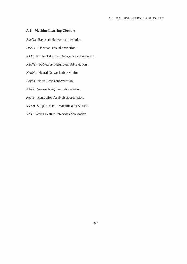
A.3. MACHINE LEARNING GLOSSARY
A.3 Machine Learning Glossary
BayNt: Bayesian Network abbreviation.
DecTr: Decision Tree abbreviation.
KLD: Kullback-Leibler Divergence abbreviation.
KNNei: K-Nearest Neighbour abbreviation.
NeuNt: Neural Network abbreviation.
Bayes: Naive Bayes abbreviation.
NNei: Nearest Neighbour abbreviation.
Regre: Regression Analysis abbreviation.
S VM: Support Vector Machine abbreviation.
VFI: Voting Feature Intervals abbreviation.
209

APPENDIX A. GLOSSARY
210
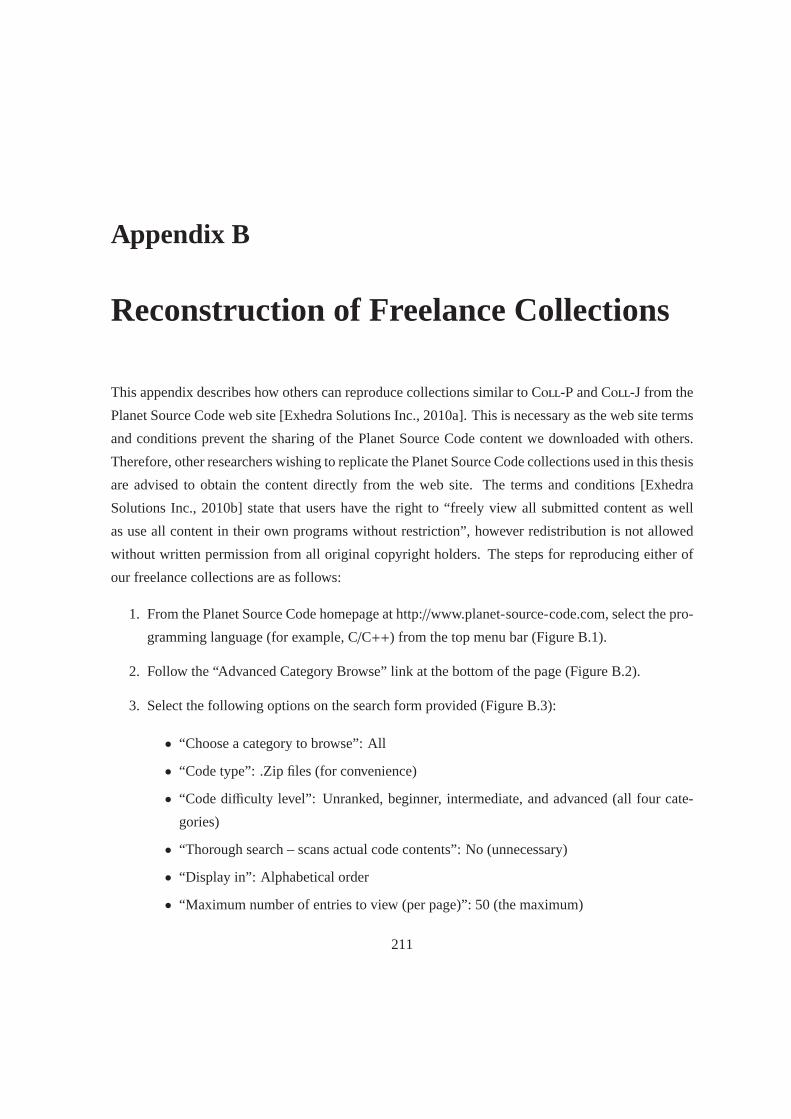
Appendix B
Reconstruction of Freelance Collections
This appendix describes how others can reproduce collections similar to Coll-P and Coll-J from the
Planet Source Code web site [Exhedra Solutions Inc., 2010a]. This is necessary as the web site terms
and conditions prevent the sharing of the Planet Source Code content we downloaded with others.
Therefore, other researchers wishing to replicate the Planet Source Code collections used in this thesis
are advised to obtain the content directly from the web site. The terms and conditions [Exhedra
Solutions Inc., 2010b] state that users have the right to “freely view all submitted content as well
as use all content in their own programs without restriction”, however redistribution is not allowed
without written permission from all original copyright holders. The steps for reproducing either of
our freelance collections are as follows:
1. From the Planet Source Code homepage at http://www.planet-source-code.com, select the pro-
gramming language (for example, C/C++) from the top menu bar (Figure B.1).
2. Follow the “Advanced Category Browse” link at the bottom of the page (Figure B.2).
3. Select the following options on the search form provided (Figure B.3):
• “Choose a category to browse”: All
• “Code type”: .Zip files (for convenience)
• “Code difficulty level”: Unranked, beginner, intermediate, and advanced (all fourcate-
gories)
• “Thorough search – scans actual code contents”: No (unnecessary)
• “Display in”: Alphabetical order
• “Maximum number of entries to view (per page)”: 50 (the maximum)
211

APPENDIX B. RECONSTRUCTION OF FREELANCE COLLECTIONS
Figure B.1: Coll-P andColl-J collection construction step 1 at Planet Source Code. Permission touse this screenshot was provided by Ian Ippolito from Exhedra Solutionson 7 May 2010.
4. Browse the result page and click on the name of any author (Figure B.4).
5. Click the “All submission(s) by this author” link (Figure B.5).
6. Check that the author has sufficient samples for your needs, and click the (zipped) work sample
links to download the samples (Figure B.6).
7. Repeat steps 4–6 above for any number of authors. Take care to record the names (or aliases) of
the authors processed to avoid duplication of effort. Use a separate folder to store the samples
for each author.
212

Figure B.2: Coll-P andColl-J collection construction step 2 at Planet Source Code. Permission touse this screenshot was provided by Ian Ippolito from Exhedra Solutionson 7 May 2010.
213

APPENDIX B. RECONSTRUCTION OF FREELANCE COLLECTIONS
Figure B.3: Coll-P andColl-J collection construction step 3 at Planet Source Code. Permission touse this screenshot was provided by Ian Ippolito from Exhedra Solutionson 7 May 2010.
214

Figure B.4: Coll-P andColl-J collection construction step 4 at Planet Source Code. Permission touse this screenshot was provided by Ian Ippolito from Exhedra Solutionson 7 May 2010.
215

APPENDIX B. RECONSTRUCTION OF FREELANCE COLLECTIONS
Figure B.5: Coll-P andColl-J collection construction step 5 at Planet Source Code. Permission touse this screenshot was provided by Ian Ippolito from Exhedra Solutionson 7 May 2010.
216

Figure B.6: Coll-P andColl-J collection construction step 6 at Planet Source Code. Permission touse this screenshot was provided by Ian Ippolito from Exhedra Solutionson 7 May 2010.
217

APPENDIX B. RECONSTRUCTION OF FREELANCE COLLECTIONS
218

Appendix C
Features from the Literature
The source code features used in previous studies with empirical contributions are organised chrono-
logically in Table C.1. We acknowledge that the feature descriptions have either been reproduced or
paraphrased for readability from the respective publications as necessary.
Table C.1 is organised into five columns. The first column contains an identification number, used
for cross-referencing purposes, consisting of the first letter of the author surname, plus a sequential
natural number.
The second column contains the identifying number (or code) used in the literature. Four of the
six contributions listed have identifying codes. Krsul [1994] and Ding andSamadzadeh [2004] used
similar numbering schemes to differentiate layout metrics, style metrics and structure metrics. Lange
and Mancoridis [2007] used metric classes such asline-len-N for calculating the percentage of
times code line lengths ofN characters appear. DiscretisingN at carefully considered lengths was
necessary for two reasons. First, we need to have a consistent value of N across all collections.
Second, these metric classes otherwise generated impractical numbers of metrics as input to the
classification algorithms. MacDonell et al. [1999] used a naming conventionsimilar to the description
of the metrics. Elenbogen and Seliya [2008] did not use codes, so we repeated the first column
identification numbers here. Kothari et al. [2007] did not use codes either, as the individual byte-
level n-grams selected do not have meaningful descriptions.
The third column contains complete descriptions of the metrics as described in theoriginal pub-
lications and modified for readability where necessary.
The fourth column documents the type of measurement for each metric. The five types of mea-
surements are: percentage measurement, integer number, real number, boolean measurement, and
one-of-many sets (or enumerations). For features with nominal measurements (boolean and set), we
chose the first-listed class descriptor in the event of measurement ties. In addition, some metrics are
219

APPENDIX C. FEATURES FROM THE LITERATURE
normalised whilst others are not. We respected the original decisions of theauthors here, even though
we believe normalisation is preferable when working with programs of varying lengths. Moreover,
we chose normalised metrics when the implementation decision is not clear.
The fifth and final column provides some tags for common notes that would otherwise be repeated
for each instance in the table. First, some of the Lange and Mancoridis [2007] metric classes such
asword-len-N have been tagged with the values ofN used. In the literature, Lange and Mancoridis
[2007] used every value ofN applicable to the collection in the study. However, the histogram-based
method proposed does not scale to a machine learning implementation with one feature for each mea-
surement. Thousands of measurements are potentially required dependingon each collection. For
example, with theline-len-N metric there could be hundreds of different line lengths in a collec-
tion, hence this metric would require hundreds of measurements in itself. Therefore we frequently
group some values ofN together (discretisation). For example, theline-len-N metric has been
documented as “N ∈ {0−19,20− ...}”, which indicates one measurement for lines of zero to nineteen
characters, and another for lines with twenty or more characters.
Some metrics require more than a shallow lexicographic parsing of the sourcecode to differen-
tiate identifiers such as local variables, global variables, function names,function parameter names,
and type definitions. Determining higher level labels for source code constructs requires success-
ful parsing of the code, and relies on correct syntax for the languagegrammar used. Given that
our anonymisation process disrupted some syntax, and that many of the source files from students
contained syntax errors anyway, we felt that parsing to identify high level features could not be suc-
cessfully automated for our collections. Use of compiler suites is a common methodfor tagging
different kinds of identifiers. For example, the Java command “javac -Xprint filename.java”
gives a list of Java methods and class variables that could be helpful forsome metrics dealing with
identifiers. We note that compiler suites are not helpful in conjunction with syntactically incorrect
samples. All collections used in this thesis are too large to be processed manually, having more work
samples than any of the previous source code authorship attribution studies, and we could not gen-
eralise their compilation for use with compiler suites. This is due to the academic collections being
selected from many semesters and courses over an eight year period, and the freelance collections
come from completely unrelated authors. For example, samples with missing compilation scripts
(such as a Makefile) could not be compiled, especially if a program requires special compilation flags
or generates multiple executables. The anonymisation process also interfered with compilation, as it
renamed all file and folder names, which consequentially broke file inclusions or similar constructs.
Finally, other samples simply contain syntax errors. We felt that any attempt atimplementing a cus-
tom parser capable of tagging all identifier types in potentially malformed software would not be
220
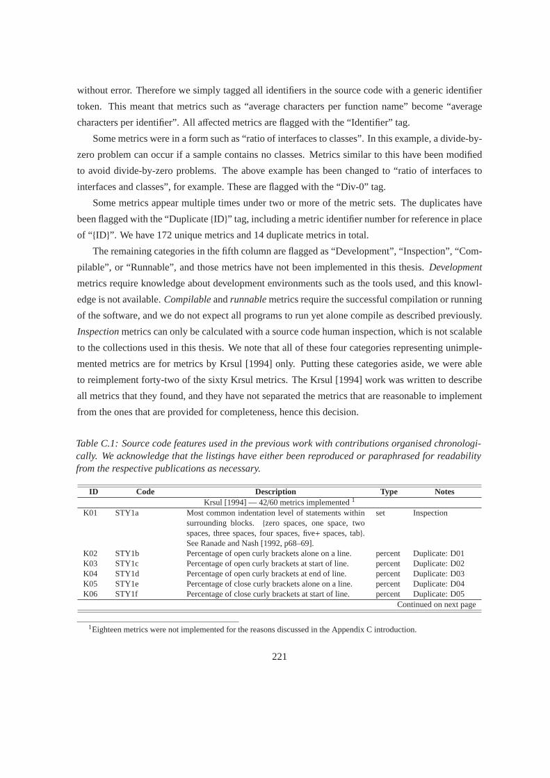
without error. Therefore we simply tagged all identifiers in the source code with a generic identifier
token. This meant that metrics such as “average characters per functionname” become “average
characters per identifier”. All affected metrics are flagged with the “Identifier” tag.
Some metrics were in a form such as “ratio of interfaces to classes”. In this example, a divide-by-
zero problem can occur if a sample contains no classes. Metrics similar to this have been modified
to avoid divide-by-zero problems. The above example has been changed to “ratio of interfaces to
interfaces and classes”, for example. These are flagged with the “Div-0” tag.
Some metrics appear multiple times under two or more of the metric sets. The duplicateshave
been flagged with the “Duplicate{ID}” tag, including a metric identifier number for reference in place
of “ {ID}”. We have 172 unique metrics and 14 duplicate metrics in total.
The remaining categories in the fifth column are flagged as “Development”, “Inspection”, “Com-
pilable”, or “Runnable”, and those metrics have not been implemented in this thesis. Development
metrics require knowledge about development environments such as the tools used, and this knowl-
edge is not available.Compilableandrunnablemetrics require the successful compilation or running
of the software, and we do not expect all programs to run yet alone compile as described previously.
Inspectionmetrics can only be calculated with a source code human inspection, which is not scalable
to the collections used in this thesis. We note that all of these four categories representing unimple-
mented metrics are for metrics by Krsul [1994] only. Putting these categoriesaside, we were able
to reimplement forty-two of the sixty Krsul metrics. The Krsul [1994] work was written to describe
all metrics that they found, and they have not separated the metrics that arereasonable to implement
from the ones that are provided for completeness, hence this decision.
Table C.1: Source code features used in the previous work with contributionsorganised chronologi-cally. We acknowledge that the listings have either been reproduced or paraphrased for readabilityfrom the respective publications as necessary.
ID Code Description Type NotesKrsul [1994] — 42/60 metrics implemented1
K01 STY1a Most common indentation level of statements withinsurrounding blocks. {zero spaces, one space, twospaces, three spaces, four spaces, five+ spaces, tab}.See Ranade and Nash [1992, p68–69].
set Inspection
K02 STY1b Percentage of open curly brackets alone on a line. percentDuplicate: D01K03 STY1c Percentage of open curly brackets at start of line. percent Duplicate: D02K04 STY1d Percentage of open curly brackets at end of line. percentDuplicate: D03K05 STY1e Percentage of close curly brackets alone on a line. percentDuplicate: D04K06 STY1f Percentage of close curly brackets at start of line. percent Duplicate: D05
Continued on next page
1Eighteen metrics were not implemented for the reasons discussed in the Appendix C introduction.
221

APPENDIX C. FEATURES FROM THE LITERATURE
Table C.1 – continued from previous page
ID Code Description Type NotesK07 STY1g Percentage of close curly brackets at end of line. percentDuplicate: D06K08 STY1h Most common indentation of open curly brack-
ets. {existing line, zero spaces, one space, twospaces, three spaces, four spaces, five+ spaces, tab}.See Ranade and Nash [1992, p68–69].
set Inspection
K09 STY1i Most common indentation of close curly brack-ets. {existing line, zero spaces, one space, twospaces, three spaces, four spaces, five+ spaces, tab}.See Ranade and Nash [1992, p68–69].
set Inspection
K10 STY2 Most common indentation style of “else” statements.{own-line, not own-line}.
set —
K11 STY3 Any variable names indented to a fixed column in vari-able declarations?
boolean Identifier,Inspection
K12 STY4 Separator between function names and parameter listsin function declarations. {spaces, carriage returns,none, mixture}.
set Identifier,Inspection
K13 STY5 Separator between function return type and functionname in function declarations.{spaces, carriage re-turns, mixture}.
set Identifier,Inspection
K14 STY6a Borders used to highlight any comments? boolean —K15 STY6b Percentage of lines of code with inline comments. percent Duplicate: M12K16 STY6c Percentage of block style comment lines to lines of
code.percent —
K17 STY7 Percentage of blank lines to lines of code. percent Duplicate: D14,Duplicate: M01
K18 PRO1 Average characters per line. real Duplicate: M06K19 PRO2a Average characters per local variable. real IdentifierK20 PRO2b Average characters per global variable. real IdentifierK21 PRO2c Average characters per function name. real Duplicate: D19,
IdentifierK22 PRO2d Average characters per function parameter name. real IdentifierK23 PRO3a Any variable names use the underscore character? boolean IdentifierK24 PRO3b Use of any temporary variables “temp”, “tmp”, or
“xxx” (case-insensitive).boolean Identifier
K25 PRO3c Percentage of variable names starting with an upper-case letter.
percent Identifier
K26 PRO3d Percentage of function names starting with an upper-case letter.
percent Identifier
K27 PRO4 Percentage of global variables to all variables. percent Identifier,Div-0
K28 PRO5 Ratio of local variables to lines of code. real IdentifierK29 PRO6 Any use of ‘#ifdef’? boolean —K30 PRO7 Most common looping construct.{for, while, do}.
(Assume “while” not counted in “do-while”.)set —
K31 PRO8 Use of any comments that near-mimic the code? boolean InspectionK32 PRO9 Most common function parameter declaration type.
{Standard C, ANSI C Java}.set Compilable
K33 PSM1 Percentage of “int” function definitions to all. percent IdentifierK34 PSM2 Percentage of “void” function definitions to all. percent IdentifierK35 PSM3 Use of any debugging symbols “debug” or “dbg”
(case-insensitive)?boolean —
Continued on next page
222
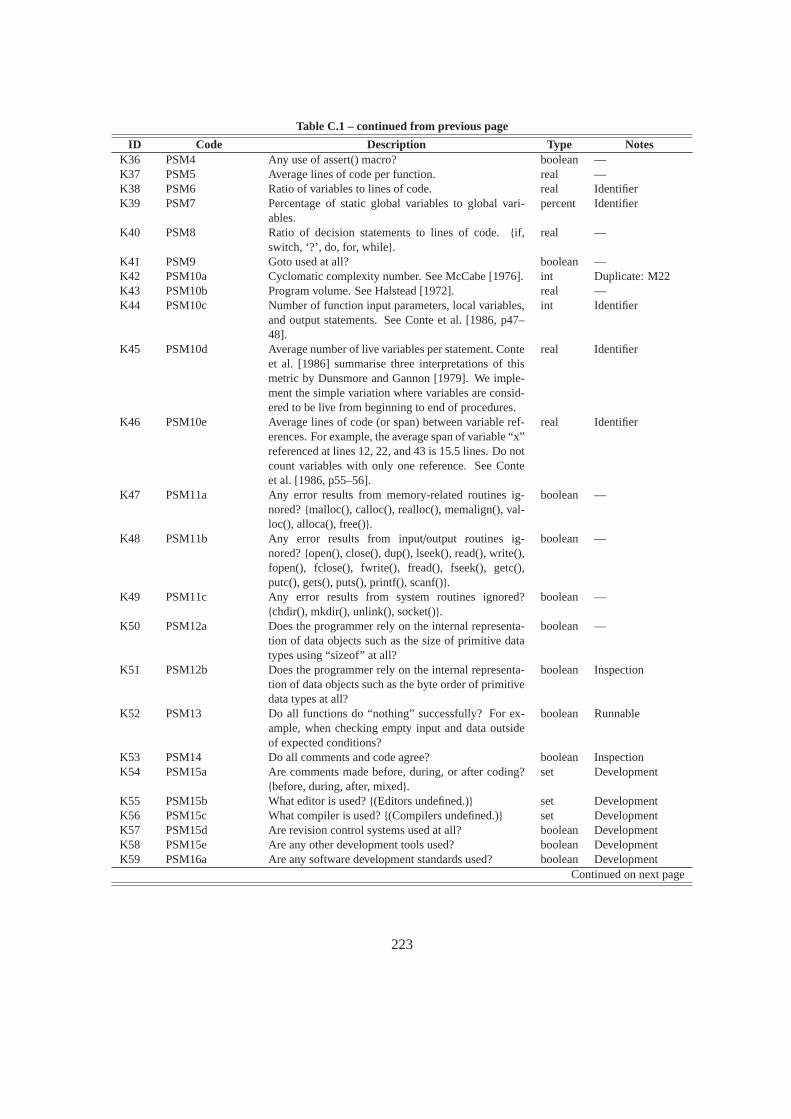
Table C.1 – continued from previous page
ID Code Description Type NotesK36 PSM4 Any use of assert() macro? boolean —K37 PSM5 Average lines of code per function. real —K38 PSM6 Ratio of variables to lines of code. real IdentifierK39 PSM7 Percentage of static global variables to global vari-
ables.percent Identifier
K40 PSM8 Ratio of decision statements to lines of code.{if,switch, ‘?’, do, for, while}.
real —
K41 PSM9 Goto used at all? boolean —K42 PSM10a Cyclomatic complexity number. See McCabe [1976]. int Duplicate: M22K43 PSM10b Program volume. See Halstead [1972]. real —K44 PSM10c Number of function input parameters, local variables,
and output statements. See Conte et al. [1986, p47–48].
int Identifier
K45 PSM10d Average number of live variables per statement. Conteet al. [1986] summarise three interpretations of thismetric by Dunsmore and Gannon [1979]. We imple-ment the simple variation where variables are consid-ered to be live from beginning to end of procedures.
real Identifier
K46 PSM10e Average lines of code (or span) between variable ref-erences. For example, the average span of variable “x”referenced at lines 12, 22, and 43 is 15.5 lines. Do notcount variables with only one reference. See Conteet al. [1986, p55–56].
real Identifier
K47 PSM11a Any error results from memory-related routines ig-nored?{malloc(), calloc(), realloc(), memalign(), val-loc(), alloca(), free()}.
boolean —
K48 PSM11b Any error results from input/output routines ig-nored?{open(), close(), dup(), lseek(), read(), write(),fopen(), fclose(), fwrite(), fread(), fseek(), getc(),putc(), gets(), puts(), printf(), scanf()}.
boolean —
K49 PSM11c Any error results from system routines ignored?{chdir(), mkdir(), unlink(), socket()}.
boolean —
K50 PSM12a Does the programmer rely on the internal representa-tion of data objects such as the size of primitive datatypes using “sizeof” at all?
boolean —
K51 PSM12b Does the programmer rely on the internal representa-tion of data objects such as the byte order of primitivedata types at all?
boolean Inspection
K52 PSM13 Do all functions do “nothing” successfully? For ex-ample, when checking empty input and data outsideof expected conditions?
boolean Runnable
K53 PSM14 Do all comments and code agree? boolean InspectionK54 PSM15a Are comments made before, during, or after coding?
{before, during, after, mixed}.set Development
K55 PSM15b What editor is used?{(Editors undefined.)} set DevelopmentK56 PSM15c What compiler is used?{(Compilers undefined.)} set DevelopmentK57 PSM15d Are revision control systems used at all? boolean DevelopmentK58 PSM15e Are any other development tools used? boolean DevelopmentK59 PSM16a Are any software development standards used? booleanDevelopment
Continued on next page
223
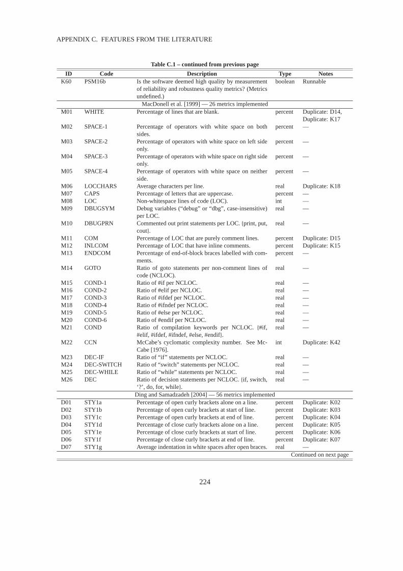
APPENDIX C. FEATURES FROM THE LITERATURE
Table C.1 – continued from previous page
ID Code Description Type NotesK60 PSM16b Is the software deemed high quality by measurement
of reliability and robustness quality metrics? (Metricsundefined.)
boolean Runnable
MacDonell et al. [1999] — 26 metrics implementedM01 WHITE Percentage of lines that are blank. percent Duplicate: D14,
Duplicate: K17M02 SPACE-1 Percentage of operators with white space on both
sides.percent —
M03 SPACE-2 Percentage of operators with white space on left sideonly.
percent —
M04 SPACE-3 Percentage of operators with white space on right sideonly.
percent —
M05 SPACE-4 Percentage of operators with white space on neitherside.
percent —
M06 LOCCHARS Average characters per line. real Duplicate: K18M07 CAPS Percentage of letters that are uppercase. percent —M08 LOC Non-whitespace lines of code (LOC). int —M09 DBUGSYM Debug variables (“debug” or “dbg”, case-insensitive)
per LOC.real —
M10 DBUGPRN Commented out print statements per LOC.{print, put,cout}.
real —
M11 COM Percentage of LOC that are purely comment lines. percent Duplicate: D15M12 INLCOM Percentage of LOC that have inline comments. percent Duplicate: K15M13 ENDCOM Percentage of end-of-block braces labelled with com-
ments.percent —
M14 GOTO Ratio of goto statements per non-comment lines ofcode (NCLOC).
real —
M15 COND-1 Ratio of #if per NCLOC. real —M16 COND-2 Ratio of #elif per NCLOC. real —M17 COND-3 Ratio of #ifdef per NCLOC. real —M18 COND-4 Ratio of #ifndef per NCLOC. real —M19 COND-5 Ratio of #else per NCLOC. real —M20 COND-6 Ratio of #endif per NCLOC. real —M21 COND Ratio of compilation keywords per NCLOC.{#if,
#elif, #ifdef, #ifndef, #else, #endif}.real —
M22 CCN McCabe’s cyclomatic complexity number. See Mc-Cabe [1976].
int Duplicate: K42
M23 DEC-IF Ratio of “if” statements per NCLOC. real —M24 DEC-SWITCH Ratio of “switch” statements per NCLOC. real —M25 DEC-WHILE Ratio of “while” statements per NCLOC. real —M26 DEC Ratio of decision statements per NCLOC.{if, switch,
‘?’, do, for, while}.real —
Ding and Samadzadeh [2004] — 56 metrics implementedD01 STY1a Percentage of open curly brackets alone on a line. percentDuplicate: K02D02 STY1b Percentage of open curly brackets at start of line. percent Duplicate: K03D03 STY1c Percentage of open curly brackets at end of line. percentDuplicate: K04D04 STY1d Percentage of close curly brackets alone on a line. percentDuplicate: K05D05 STY1e Percentage of close curly brackets at start of line. percent Duplicate: K06D06 STY1f Percentage of close curly brackets at end of line. percentDuplicate: K07D07 STY1g Average indentation in white spaces after open braces. real —
Continued on next page
224
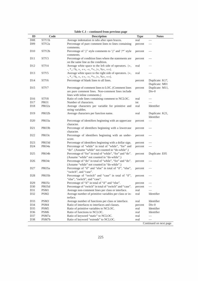
Table C.1 – continued from previous page
ID Code Description Type NotesD08 STY1h Average indentation in tabs after open braces. real —D09 STY2a Percentage of pure comment lines to lines containing
comments.percent —
D10 STY2b Percentage of ‘//’ style comments to ‘//’ and ‘/*’ stylecomments.
percent —
D11 STY3 Percentage of condition lines where the statements areon the same line as the condition.
percent —
D12 STY4 Average white space to the left side of operators.{+,-, *, /%,=, +=, -=, *=, /=, %=, ==}.
real —
D13 STY5 Average white space to the right side of operators.{+,-, *, /%,=, +=, -=, *=, /=, %=, ==}.
real —
D14 STY6 Percentage of blank lines to all lines. percent Duplicate: K17,Duplicate: M01
D15 STY7 Percentage of comment lines to LOC. (Comment linesare pure comment lines. Non-comment lines includelines with inline comments.)
percent Duplicate: M11,Div-0
D16 STY8 Ratio of code lines containing comment to NCLOC. real —D17 PRO1 Number of characters. int —D18 PRO2a Average characters per variable for primitive and
string variables.real Identifier
D19 PRO2b Average characters per function name. real Duplicate: K21,Identifier
D20 PRO3a Percentage of identifiers beginning with an uppercasecharacter.
percent —
D21 PRO3b Percentage of identifiers beginning with a lowercasecharacter.
percent —
D22 PRO3c Percentage of identifiers beginning with an under-score.
percent —
D23 PRO3d Percentage of identifiers beginning with a dollar sign. percent—D24 PRO4a Percentage of “while” in total of “while”, “for” and
“do”. (Assume “while” not counted in “do-while”.)percent —
D25 PRO4b Percentage of “for” in total of “while”, “for” and “do”.(Assume “while” not counted in “do-while”.)
percent Duplicate: E05
D26 PRO4c Percentage of “do” in total of “while”, “for” and “do”.(Assume “while” not counted in “do-while”.)
percent —
D27 PRO5a Percentage of “if” and “else” in total of “if”, “else”,“switch”, and “case”.
percent —
D28 PRO5b Percentage of “switch” and “case” in total of “if”,“else”, “switch”, and “case”.
percent —
D29 PRO5c Percentage of “if” in total of “if” and “else”. percent —D30 PRO5d Percentage of “switch” in total of “switch” and “case”. percent —D31 PSM1 Average non-comment lines per class or interface. real —D32 PSM2 Average number of primitive variables per class or in-
terface.real Identifier
D33 PSM3 Average number of functions per class or interface. real IdentifierD34 PSM4 Ratio of interfaces to interfaces and classes. percent Div-0D35 PSM5 Ratio of primitive variables to NCLOC. real IdentifierD36 PSM6 Ratio of functions to NCLOC. real IdentifierD37 PSM7a Ratio of keyword “static” to NCLOC. real —D38 PSM7b Ratio of keyword “extends” to NCLOC. real —
Continued on next page
225

APPENDIX C. FEATURES FROM THE LITERATURE
Table C.1 – continued from previous page
ID Code Description Type NotesD39 PSM7c Ratio of keyword “class” to NCLOC. real —D40 PSM7d Ratio of keyword “abstract” to NCLOC. real —D41 PSM7e Ratio of keyword “implements” to NCLOC. real —D42 PSM7f Ratio of keyword “import” to NCLOC. real —D43 PSM7g Ratio of keyword “instanceof” to NCLOC. real —D44 PSM7h Ratio of keyword “interface” to NCLOC. real —D45 PSM7i Ratio of keyword “native” to NCLOC. real —D46 PSM7j Ratio of keyword “new” to NCLOC. real —D47 PSM7k Ratio of keyword “package” to NCLOC. real —D48 PSM7l Ratio of keyword “private” to NCLOC. real —D49 PSM7m Ratio of keyword “public” to NCLOC. real —D50 PSM7n Ratio of keyword “protected” to NCLOC. real —D51 PSM7o Ratio of keyword “this” to NCLOC. real —D52 PSM7p Ratio of keyword “super” to NCLOC. real —D53 PSM7q Ratio of keyword “try” to NCLOC. real —D54 PSM7r Ratio of keyword “throw” to NCLOC. real —D55 PSM7s Ratio of keyword “catch” to NCLOC. real —D56 PSM7t Ratio of keyword “final” to NCLOC. real —
Lange and Mancoridis [2007] — 56 metrics implemented2
L01 access-1 Percent of keyword “public” to all access statements. percent Div-0L02 access-2 Percent of keyword “protected” to all access state-
ments.percent Div-0
L03 access-3 Percent of keyword “private” to all access statements. percent Div-0L04 brace-pos-1 Percentage of open curly brace on own line to all brace
position placements.percent Div-0
L05 brace-pos-2 Percentage of open curly brace as the leftmost non-whitespace character on a line to all brace positionplacements.
percent Div-0
L06 brace-pos-3 Percentage of open curly brace on the interior of non-whitespace characters on a line to all brace positionplacements.
percent Div-0
L07 brace-pos-4 Percentage of open curly brace as the rightmost non-whitespace character on a line to all brace positionplacements.
percent Div-0
L08 brace-pos-5 Percentage of close curly brace on own line to allbrace position placements.
percent Div-0
L09 brace-pos-6 Percentage of close curly brace as the leftmost non-whitespace character on a line to all brace positionplacements.
percent Div-0
L10 brace-pos-7 Percentage of close curly brace on the interior of non-whitespace characters on a line to all brace positionplacements.
percent Div-0
L11 brace-pos-8 Percentage of close curly brace as the rightmost non-whitespace character on a line to all brace positionplacements.
percent Div-0
Continued on next page
2Some of these metrics are in the formatname-N. Taking line-len-N for example,N represents the normalisedfrequency of all recorded line lengths for 0..N characters. Therefore we document these in groups (or classes) for brevity.In addition, the maximum value forN depends on the data, but we have only implemented thirty metrics from the fourteenmetric classes. We grouped many values ofN together to keep the feature space manageable. This process is known asdiscretisation.
226

Table C.1 – continued from previous page
ID Code Description Type NotesL12 comment-1 Percentage of block comments to all comments. percent—L13 comment-2 Percentage of line comments to all comments. percent —L14 comment-3 Percentage of JavaDoc comments to all comments. percent —L15 control-flow-1 Percentage of “for” statement to all control flow state-
ments.percent Div-0
L16 control-flow-2 Percentage of “foreach” statement to all control flowstatements.
percent Div-0
L17 control-flow-3 Percentage of “while” statement to all control flowstatements.
percent Div-0
L18 control-flow-4 Percentage of “do” statement to all control flow state-ments.
percent Div-0
L19 control-flow-5 Percentage of “if” statement to all control flow state-ments.
percent Div-0
L20 control-flow-6 Percentage of “switch” statement to all control flowstatements.
percent Div-0
L21 control-flow-7 Percentage of “throw” statement to all control flowstatements.
percent Div-0
L22 control-flow-8 Percentage of function calls to all control flow state-ments.
percent Identifier,Div-0
L23N indent-space-N Normalised frequency of chunks of N spaces for in-dentation at start of line.
percent N ∈ {0,1− ...}
L24N indent-tab-N Normalised frequency of chunks of N tabs for inden-tation at start of line.
percent N ∈ {0,1− ...}
L25N inline-space-N Normalised frequency of chunks of N spaces for inter-nal spacing purposes.
percent N ∈ {1,2− ...}
L26N inline-tab-N Normalised frequency of chunks of N tabs for internalspacing purposes.
percent N ∈ {1,2− ...}
L27N trail-space-N Normalised frequency of chunks of N spaces at end ofline.
percent N ∈ {0,1− ...}
L28N trail-tab-N Normalised frequency of chunks of N tabs at end ofline.
percent N ∈ {0,1− ...}
L29N period-N Normalised frequency of periods in single logicalidentifiers. Example: a.b.c().d().
percent N ∈ {1,2− ...}
L30N underscore-N Normalised frequency of identifiers with N under-scores.
percent N ∈ {1,2− ...}
L31N switch-N Normalised frequency of “switch” blocks with N“case” groups.
percent N ∈ {1−2,3− ...}
L32N switch-case-N Normalised frequency of “switch” blocks with N“case” statements.
percent N ∈ {1−2,3− ...}
L33N line-words-N Normalised frequency of lines with N words. (Awordis a sequence of characters separated by white space.)
percent N ∈ {0−2,3− ...}
L34N word-first-char-N Normalised frequency of identifiers beginning withthe integer value N of the first character. Fifty-fourmetrics could be implemented for the applicable char-acters:{a-z, A-Z, , $}. Our implementation uses fourmetrics representing character classes for lowercasecharacters (N = 1), uppercase characters (N = 2), un-derscores (N = 3), and dollar signs (N = 4) to reducethe number or metrics.
percent N ∈ {1,2,3,4}
L35N word-len-N Normalised frequency of identifiers of length N. percent N ∈ {1−5,6− ...}Continued on next page
227

APPENDIX C. FEATURES FROM THE LITERATURE
Table C.1 – continued from previous page
ID Code Description Type NotesL36N line-len-N Normalised frequency of lines of length N. percentN ∈ {1−19,20− ...}K01N commas-N Normalised frequency of lines with N commas. percentN ∈ {0,1− ...}K02N semicolons-N Normalised frequency of lines with N semicolons. percent N ∈ {0,1− ...}
Elenbogen and Seliya [2008] — 6 metrics implementedE01 1 Number of lines of code. int —E02 2 Number of comments. int —E03 3 Average length of variable names. real —E04 4 Number of variables. int —E05 5 Percent of “for” loop constructs to all looping con-
structs. (Assume “while” not counted in “do-while”.)percent Duplicate: D25
E06 6 Number of bits in the zipped program using WinZip.We used a Unix-based zip implementation.
int —
Kothari et al. [2007] — 168 metrics implementedThe metric set comprises the normalised frequencies of the 50 most common byte-level n-grams for each author.
228

Appendix D
Programming Language Feature Tables
Tables D.1, D.2, and D.3 present operator and keyword tables for C, C++, and Java respectively,
as used for source code features as discussed in Section 5.1.2 (p. 111). Overloaded operators are
only listed once using their most common form. Tables D.4 and D.5 additionally present C lan-
guage input/output keywords, function words, white space tokens, and literal features as discussed in
Section 5.3 (p. 122).
229

APPENDIX D. PROGRAMMING LANGUAGE FEATURE TABLES
Operators( parenthesis != not equals[ bracket & bitwise and-> indirect member access ˆ bitwise xor. member access | bitwise or++ increment && boolean and-- decrement || boolean or! not ? conditional˜ complement = equals* multiply += plus equals/ divide -= minus equals% modulo *= multiply equals+ plus /= divide equals- minus %= modulo equals<< left shift <<= left shift equals>> right shift >>= right shift equals< less than &= bitwise and equals> greater than ˆ= bitwise xor equals<= less than equals |= bitwise or equals>= greater than equals , comma== equality
Keywordsauto do goto signed unsigned
break double if sizeof void
case else int static volatile
char enum long struct while
const extern register switch
continue float return typedef
default for short union
Table D.1: C language operators and keywords [Kelly and Pohl, 1997] preserved in samples inColl-A andColl-T.
230

Operators->* bind pointer to member by pointer :: scope resolution.* bind pointer to member by reference
Keywordsasm export private true
bool false protected try
catch friend public typeid
class inline reinterpret_cast typename
const_cast mutable static_cast using
delete namespace template virtual
dynamic_cast new this wchar_t
explicit operator throw
Table D.2: C++ operators [Farrell, 2008] and keywords [International Standardization Organizationand International Electrotechnical Commission, 1998] preserved in samples inColl-P. This tabledoes not duplicate operators and keywords that appear in both C and C++ languages as documentedin Table D.1.
231

APPENDIX D. PROGRAMMING LANGUAGE FEATURE TABLES
Operators( parenthesis != not equals[ bracket & bitwise and. member access ˆ bitwise xor++ increment | bitwise or-- decrement && boolean and! not || boolean or˜ complement ? conditional* multiply = equals/ divide += plus equals% modulo -= minus equals+ plus *= multiply equals- minus /= divide equals<< left shift %= modulo equals>> right shift† <<= left shift equals>>> right shift‡ >>= right shift equals†
< less than >>>= right shift equals‡
> greater than &= bitwise and equals<= less than equals ˆ= bitwise xor equals>= greater than equals |= bitwise or equals== equality
Keywordsabstract continue float new switch
assert default goto package synchronized
boolean do if private this
break double implements protected throw
byte else import public throws
case enum instanceof return transient
catch extends int short try
char for interface static void
class final long strictfp volatile
const finally native super while
Table D.3: Java operators [Liang, 2006] and keywords [Lindsey et al., 2005] preserved in samplesin Coll-J. (†Right shift with sign extension.‡Right shift with zero extension.)
232

Feature Class 1: KeywordsSee Table D.1.
Feature Class 2: OperatorsSee Table D.1.
Feature Class 3: Input/Output Keywords [Huss, 1997]BUFSIZ FILE fscanf _IONBF rewind stderr
clearerr FILENAME_MAX fseek L_tmpnam scanf stdin
EOF fopen fsetpos NULL SEEK_CUR stdout
fclose FOPEN_MAX ftell perror SEEK_END tmpfile
feof fpos_t fwrite printf SEEK_SET TMP_MAX
ferror fprintf getc putc setbuf tmpnam
fflush fputc getchar putchar setvbuf ungetc
fgetc fputs gets puts size_t vfprintf
fgetpos fread _IOFBF remove sprintf vprintf
fgets freopen _IOLBF rename sscanf vsprintf
Feature Class 4: Function WordsSee Table D.5.
Feature Class 5: White Space Tokens‘ ’ space ‘\t’ tab ‘\r’ carriage return ‘\n’ new line
Feature Class 6: LiteralsRegular expression Literal name Example[a-z]+ Lowercase literal thisisanexample
[A-Z]+ Uppercase literal THISISANEXAMPLE
[a-z][a-zA-Z]+ Camelcase literal thisIsAnExample
[A-Z][a-zA-Z]+ Titlecase literal ThisIsAnExample
[a-zA-Z_][a-zA-Z0-9_]+ Other literal _this_IS_anEXAMPLE_123
Table D.4: Six feature classes and corresponding features that were used in feature selection experi-ments in Section 5.3 (p. 122).
233

APPENDIX D. PROGRAMMING LANGUAGE FEATURE TABLES
Feature Class 4: Function Wordsabort ERANGE isxdigit memcpy strcmp
abs errno jmp_buf memmove strcoll
acos exit labs memset strcpy
asctime EXIT_FAILURE LC_ALL mktime strcspn
asin EXIT_SUCCESS LC_COLLATE modf strerror
assert exp LC_CTYPE NDEBUG strftime
atan fabs LC_MONETARY offsetof strlen
atan2 floor LC_NUMERIC pow strncat
atexit FLT_DIG lconv ptrdiff_t strncmp
atof FLT_EPSILON LC_TIME qsort strncpy
atoi FLT_MANT_DIG LDBL_DIG raise strpbrk
atol FLT_MAX LDBL_EPSILON rand strrchr
bsearch FLT_MAX_10_EXP LDBL_MANT_DIG RAND_MAX strspn
calloc FLT_MAX_EXP LDBL_MAX realloc strstr
ceil FLT_MIN LDBL_MAX_10_EXP SCHAR_MAX strtod
CHAR_BIT FLT_MIN_10_EXP LDBL_MAX_EXP SCHAR_MIN strtok
CHAR_MAX FLT_MIN_EXP LDBL_MIN setjmp strtol
CHAR_MIN FLT_RADIX LDBL_MIN_10_EXP setlocale strtoul
clock FLT_ROUNDS LDBL_MIN_EXP SHRT_MAX strxfrm
CLOCKS_PER_SEC fmod ldexp SHRT_MIN system
clock_t free ldiv SIGABRT tan
cos frexp ldiv_t sig_atomic_t tanh
cosh getenv localeconv SIG_DFL time
ctime gmtime localtime SIG_ERR tm
DBL_DIG HUGE_VAL log SIGFPE tolower
DBL_EPSILON INT_MAX log10 SIG_IGN toupper
DBL_MANT_DIG INT_MIN longjmp SIGILL UCHAR_MAX
DBL_MAX isalnum LONG_MAX SIGINT UINT_MAX
DBL_MAX_10_EXP isalpha LONG_MIN signal ULONG_MAX
DBL_MAX_EXP iscntrl malloc SIGSEGV USHRT_MAX
DBL_MIN isdigit MB_CUR_MAX SIGTERM va_arg
DBL_MIN_10_EXP isgraph mblen sin va_end
DBL_MIN_EXP islower MB_LEN_MAX sinh va_list
difftime isprint mbstowcs sqrt va_start
div ispunct mbtowc srand wchar_t
div_t isspace memchr strcat wcstombs
EDOM isupper memcmp strchr wctomb
Table D.5: “Feature Class 4: Function Words” content [Huss, 1997] referenced in Table D.4 movedhere for space.
234

Bibliography
A. Aamodt and E. Plaza. Case-based reasoning: Foundational issues, methodological variations, and
system approaches.AI Communications, 7(1):39–59, March 1994.
H. Abdi. The bonferonni and sidak corrections for multiple comparisons.In N. J. Salkind, editor,
Encyclopedia of Measurement and Statistics, pages 103–107. Sage Publications Inc., Thousand
Oaks, California, October 2006.
T. Abou-Assaleh, N. Cercone, V. Keselj, and R. Sweidan. N-gram-based detection of new malicious
code. In P. Cheung, E. Wong, and K. Kanoun, editors,Proceedings of the Twenty-Eighth Annual
IEEE International Computer Software and Applications Conference, pages 41–42, Hong Kong,
China, September 2004a. IEEE Computer Society Press.
T. Abou-Assaleh, N. Cercone, V. Keselj, and R. Sweidan. Detection ofnew malicious code using
n-grams signatures. In E. Keizer, G. Sprague, and S. Marsh, editors, Proceedings of the Second
Annual Conference on Privacy, Security and Trust, pages 193–196, Fredericton, Canada, October
2004b. University of New Brunswick.
T. Abraham and O. de Vel. Investigative profiling with computer forensic log data and association
rules. In N. Zhong, P. S. Yu, V. Kumar, and S. Tsumoto, editors,Proceedings of the Second IEEE
International Conference on Data Mining, pages 11–18, Maebashi, Japan, December 2002. IEEE
Computer Society Press.
A. Adelsbach and A. Reza Sadeghi. Advanced techniques for dispute resolving and authorship proofs
on digital works. In E. J. Delp and P. W. Wong, editors,Proceedings of the Fifth Conference
on Security and Watermarking of Multimedia Contents, pages 677–688, Santa Clara, California,
January 2003. International Society for Optical Engineering.
235
BIBLIOGRAPHY
A. Alemozafar. Online software battles plagiarism at Stanford. The Stanford Daily, February 2003.
URL: http://www.stanforddaily.com/2003/02/12/online-software-battles-plagiarism-at-stanford
[Accessed 16 August 2010].
American Psychological Association.Publication Manual of the American Psychological Associa-
tion. American Psychological Association, Washington, D.C., sixth edition, July 2009.
E. Amitay, S. Yogev, and E. Yom-Tov. Serial sharers: Detecting split identities of web authors. In
B. Stein, M. Koppel, and E. Stamatatos, editors,Proceedings of the First International Workshop
on Plagiarism Analysis, Authorship Identification, and Near-Duplicate Detection, pages 11–18,
Amsterdam, Netherlands, July 2007. CEUR Workshop Proceedings.
J. R. Anderson, R. Farrell, and R. Sauers. Learning to program in Lisp. Cognitive Science, 8(2):
87–129, April 1984.
V. N. Anh and A. Moffat. Inverted index compression using word-aligned binary codes.Information
Retrieval, 8(1):151–166, January 2005.
A. Arasu, J. Cho, H. Garcia-Molina, A. Paepcke, and S. Raghavan.Searching the web.ACM Trans-
actions on Internet Technology, 1(1):2–43, August 2001.
S. Argamon, M. Koppel, J. Fine, and A. R. Shimoni. Gender, genre, andwriting style in formal
written texts.Text — Interdisciplinary Journal for the Study of Discourse, 23(3):321–346, August
2003a.
S. Argamon, M. Saric, and S. S. Stein. Style mining of electronic messages for multiple authorship
discrimination: First results. In L. Getoor, T. Senator, P. Domingos, and C. Faloutsos, editors,
Proceedings of the Ninth ACM SIGKDD International Conference on Knowledge Discovery and
Data Mining, pages 475–480, Washington, D.C., August 2003b. ACM Press.
C. Arwin and S. M. M. Tahaghoghi. Plagiarism detection across programming languages. In
V. Estivill-Castro and G. Dobbie, editors,Proceedings of the Twenty-Ninth Australasian Com-
puter Science Conference, pages 277–286, Hobart, Australia, January 2006. Australian Computer
Society.
Assignment Centre. Australia’s & NZ leading education assignments help company, June 2009.
URL: http://www.assignmentcentre.com.au [Accessed 23 February 2010].
Y. Bae Lee and S. H. Myaeng. Text genre classification with genre-revealing and subject-revealing
features. In K. Jarvelin, M. Beaulieu, R. Baeza-Yates, and S. H. Myaeng, editors,Proceedings of
236

BIBLIOGRAPHY
the Twenty-Fifth Annual International ACM SIGIR Conference on Research and Development in
Information Retrieval, pages 145–150, Tampere, Finland, August 2002. ACM Press.
R. Baeza-Yates and B. Ribeiro-Neto.Modern Information Retrieval. Addison Wesley Longman,
Reading, Massachusetts, first edition, May 1999.
D. Bahle, H. E. Williams, and J. Zobel. Efficient phrase querying with an auxiliary index. In
K. Jarvelin, M. Beaulieu, R. Baeza-Yates, and S. H. Myaeng, editors,Proceedings of the Twenty-
Fifth Annual International ACM SIGIR Conference on Research and Development in Information
Retrieval, pages 215–221, Tampere, Finland, August 2002. ACM Press.
P. Bame. McCabe-style function complexity and line counting for C and C++, March 2010.
URL: http://www.parisc-linux.org/∼bame/pmccabe [Accessed 1 March 2010].
A. Barron-Cedeno, P. Rosso, and J. Miguel Benedi. Reducing the plagiarism detection search space
on the basis of the Kullback-Leibler distance. In A. Gelbukh, editor,Proceedings of the Tenth Inter-
national Conference on Computational Linguistics and Intelligent Text Processing, pages 523–534,
Mexico City, Mexico, March 2009. Springer.
E. Bauer and R. Kohavi. An empirical comparison of voting classification algorithms: Bagging,
boosting, and variants.Machine Learning, 36(2):105–139, August 1999.
L. A. Becker. Effect size, March 2000. URL: http://www.uccs.edu/∼faculty/lbecker/es.htm [Accessed
2 September 2010].
B. Belkhouche, A. Nix, and J. Hassell. Plagiarism detection in software designs. In S. Moo Yoo and
L. H. Etzkorn, editors,Proceedings of the Forty-Second Annual Southeast Regional Conference,
pages 207–211, Huntsville, Alabama, April 2004. ACM Press.
C. H. Bennett, M. Li, and B. Ma. Chain letters & evolutionary histories.Scientific American, 288(6):
76–81, June 2003.
Y. Bernstein, B. Billerbeck, S. Garcia, N. Lester, F. Scholer, J. Zobel, and W. Webber. RMIT Uni-
versity at TREC 2005: Terabyte and robust track. In E. M. Voorheesand L. P. Buckland, editors,
Proceedings of the Fourteenth Text Retrieval Conference, pages 1–12, Gaithersburg, Maryland,
November 2005. National Institute of Standards and Technology.
D. Biber. Representativeness in corpus design.Literary and Linguistic Computing, 8(4):243–257,
December 1993.
237

BIBLIOGRAPHY
B. Bollag. Edward waters college loses accreditation following plagiarism scandal. The Chronicle of
Higher Education, December 2004. URL: http://chronicle.com/prm/daily/2004/12/2004120904n.
htm [Accessed 8 October 2007].
R. A. Bosch and J. A. Smith. Separating hyperplanes and the authorship of the disputed Federalist
papers.The American Mathematical Monthly, 105(7):601–608, August 1998.
K. W. Bowyer and L. O. Hall. Experience using MOSS to detect cheating onprogramming assign-
ments. In D. Budny, R. V. Espinosa, L. G. Richards, and T. L. Skvarenina, editors,Proceedings of
the Twenty-Ninth ASEE/IEEE Frontiers in Education Conference, pages 18–22, San Juan, Puerto
Rico, November 1999. IEEE Computer Society Press.
M. D. S. Braine. The ontogeny of English phrase structure: The first phase.Language, 39(1):1–13,
January 1963.
S. Brin and L. Page. The anatomy of a large-scale hypertextual web search engine. In H. Ashman
and P. Thistlewaite, editors,Proceedings of the Seventh International World Wide Web Conference,
pages 107–117, Brisbane, Australia, April 1998. Elsevier Science Publishers Ltd.
A. Z. Broder. On the resemblance and containment of documents. In B. Carpentieri, A. De Santis,
U. Vaccaro, and J. A. Storer, editors,Proceedings of the First International Conference on Com-
pression and Complexity of Sequences, pages 21–29, Positano, Italy, June 1998. IEEE Computer
Society Press.
A. Z. Broder. Identifying and filtering near-duplicate documents. In R. Giancarlo and D. Sankoff,
editors,Proceedings of the Eleventh Annual Symposium on Combinatorial Pattern Matching, pages
1–10, Montreal, Canada, June 2000. Springer.
A. Z. Broder, M. Charikar, A. M. Frieze, and M. Mitzenmacher. Min-wise independent permuta-
tions. In J. Vitter, editor,Proceedings of the Thirtieth Annual ACM Symposium on the Theory of
Computing, pages 327–336, Dallas, Texas, May 1998. ACM Press.
J. Bull, C. Collins, E. Coughlin, and D. Sharp. Technical review of plagiarism detection software
report. Technical Report LU1 3JU, Computer Assisted Assessment Centre, University of Luton,
Bedfordshire, United Kingdom, July 2002.
J. D. Burger and J. C. Henderson. An exploration of observable features related to blogger age. In
N. Nicolov, F. Salvetti, M. Liberman, and J. H. Martin, editors,Proceedings of the Fourteenth
238

BIBLIOGRAPHY
AAAI Spring Symposium on Computational Approaches to Analysing Weblogs, pages 15–20, Palo
Alto, California, March 2006. Association for the Advancement of Artificial Intelligence.
S. Burrows and S. M. M. Tahaghoghi. Source code authorship attribution using n-grams. In A. Spink,
A. Turpin, and M. Wu, editors,Proceedings of the Twelfth Australasian Document Computing
Symposium, pages 32–39, Melbourne, Australia, December 2007. RMIT University.
S. Burrows, A. L. Uitdenbogerd, and A. Turpin. Authorship attribution of source code. In submission.
S. Burrows, S. M. M. Tahaghoghi, and J. Zobel. Efficient plagiarism detection for large code reposi-
tories.Software: Practice and Experience, 37(2):151–175, September 2006.
S. Burrows, A. L. Uitdenbogerd, and A. Turpin. Application of information retrieval techniques
for source code authorship attribution. In X. Zhou, H. Yokota, R. Kotagiri, and X. Lin, editors,
Proceedings of the Fourteenth International Conference on Database Systems for Advanced Ap-
plications, pages 699–713, Brisbane, Australia, April 2009a. Springer.
S. Burrows, A. L. Uitdenbogerd, and A. Turpin. Temporally robust software features for authorship
attribution. In T. Hey, E. Bertino, V. Getov, and L. Liu, editors,Proceedings of the Thirty-Third An-
nual IEEE International Computer Software and Applications Conference, pages 599–606, Seattle,
Washington, July 2009b. IEEE Computer Society Press.
F. Can and J. M. Patton. Change of writing style with time.Computers and the Humanities, 38(1):
61–82, February 2004.
L. W. Cannon, R. A. Elliott, L. W. Kirchhoff, J. H. Miller, J. M. Miller, R. W. Mitze, E. P. Schan,
N. O. Whittington, H. Spencer, D. Keppel, and M. Brader. Recommended Cstyle and coding
standards. Technical Report Version 6.0, Bell Labs, Murray Hill, NewJersey, University of
Toronto, Toronto, Canada, University of Washington, Seattle, Washington, and SoftQuad Incor-
porated, Toronto, Canada, February 1997.
W. B. Cavnar and J. M. Trenkle. N-gram-based text categorisation. InProceedings of the Third
Annual Symposium on Document Analysis and Information Retrieval, pages 161–175, Las Vegas,
Nevada, April 1994. Center of Excellence for Document Analysis and Recognition.
P. Clough and M. Stevenson. Creating a corpus of plagiarised academic texts. In M. Mahlberg, editor,
Proceedings of the Fifth Corpus Linguistics Conference, pages 1–14, Liverpool, United Kingdom,
July 2009. University of Liverpool.
239

BIBLIOGRAPHY
P. Clough, R. Gaizauskas, and S. L. Piao. Building and annotating a corpus for the study of jour-
nalistic text reuse. In A. Zampolli, editor,Proceedings of the Third International Conference on
Language Resources and Evaluation, pages 1678–1691, Los Palmas, Spain, May 2002. European
Language Resources Association.
J. Cohen.Statistical Power Analysis for the Behavioral Sciences. Lawrence Erlbaum Associates Inc.,
Hillsdale, New Jersey, second edition, January 1988.
F. Colas, P. Paclik, J. N. Kok, and P. Brazdil. Does SVM really scale up tolarge bag of words feature
spaces? In M. R. Berthold, J. Shawe-Taylor, and N. Lavrac, editors, Proceedings of the Sev-
enth International Symposium on Intelligent Data Analysis, pages 296–307, Ljubljana, Slovenia,
September 2007. Springer.
C. Collberg and S. Kobourov. Self-plagiarism in computer science.Communications of the ACM, 48
(4):88–94, April 2005.
S. D. Conte, H. E. Dunsmore, and V. Y. Shen.Software Engineering Metrics and Models. Ben-
jamin/Cummings Publishing Inc., Redwood City, California, first edition, March 1986.
M. Cook. Experimenting to produce a software tool for authorship attribution. Technical Report
COM3021, Department of Computer Science, University of Sheffield, Sheffield, United Kingdom,
May 2003.
F. Culwin, A. MacLeod, and T. Lancaster. Source code plagiarism in UK HE computing schools:
Issues, attitudes and tools. Technical Report SBU-CISM-01-01, South Bank University School of
Computing, Information Systems and Mathematics, London, United Kingdom, September 2001.
S. J. Cunningham, J. Littin, and I. H. Witten. Applications of machine learning ininformation re-
trieval. Working Paper Series, 97(6):1–48, February 1997.
Custom Writing. Custom essay writing service, February 2009. URL: http://custom-writing.org
[Accessed 24 February 2009].
M. M. Dalkilic, W. T. Clark, J. C. Costello, and P. Radivojac. Using compression to identify classes
of inauthentic texts. In J. Ghosh, D. Lambert, D. Skillicorn, and J. Srivastava, editors,Proceedings
of the Sixth SIAM International Conference on Data Mining, pages 604–608, Bethesda, Maryland,
April 2006. Society for Industrial and Applied Mathematics.
C. Daly and J. Horgan. A technique for detecting plagiarism in computer code. The Computer
Journal, 48(6):662–666, November 2005.
240

BIBLIOGRAPHY
O. de Vel, A. Anderson, M. Corney, and G. Mohay. Mining e-mail content for author identification
forensics.SIGMOD Record, 30(4):55–64, December 2001.
G. Demiroz and H. A. Guvenir. Classification by voting feature intervals. InM. van Someren and
G. Widmer, editors,Proceedings of the Ninth European Conference on Machine Learning, pages
85–92, Prague, Czech Republic, April 1997. Springer.
M. Dick, J. Sheard, C. Bareiss, J. Carter, D. Joyce, T. Harding, and C. Laxer. Addressing student
cheating: Definitions and solutions.ACM SIGCSE Bulletin, 35(2):172–184, June 2003.
J. Diederich, J. Kindermann, E. Leopold, and G. Paass. Authorship attribution with support vector
machines.Applied Intelligence, 19(1–2):109–123, May 2003.
E. W. Dijkstra. Go to statement considered harmful.Communications of the ACM, 11(3):147–148,
March 1968.
H. Ding and M. H. Samadzadeh. Extraction of Java program fingerprintsfor software authorship
identification.Journal of Systems and Software, 72(1):49–57, June 2004.
J. L. Donaldson, A. Marie Lancaster, and P. H. Sposato. A plagiarism detection system. In K. I.
Magel, F. G. Walters, and N. B. Dale, editors,Proceedings of the Twelfth SIGCSE Technical Sym-
posium on Computer Science Education, pages 21–25, St. Louis, Missouri, February 1981. ACM
Press.
H. Drucker, D. Wu, and V. N. Vapnik. Support vector machines for spam categorisation.IEEE
Transactions on Neural Networks, 10(5):1048–1054, September 1999.
D. D’Souza, M. Hamilton, and M. Harris. Software development marketplaces — implications for
plagiarism. In S. Mann and Simon, editors,Proceedings of the Ninth Australasian Computing Ed-
ucation Conference, pages 27–33, Ballarat, Australia, January 2007. Australian Computer Society.
H. E. Dunsmore and J. D. Gannon. Data referencing: An empirical investigation. Computing, 12
(12):50–59, December 1979.
B. S. Elenbogen and N. Seliya. Detecting outsourced student programmingassignments.Journal of
Computing Sciences in Colleges, 23(3):50–57, January 2008.
W. E. Y. Elliott and R. J. Valenza. Was the Earl of Oxford the true Shakespeare? A computer-aided
analysis.Notes and Queries, 38(4):501–506, December 1991.
241

BIBLIOGRAPHY
W. E. Y. Elliott and R. J. Valenza. And then there were none: Winnowing theshakespeare claimants.
Computers and the Humanities, 30(3):191–245, May 1996.
S. Engels, V. Lakshmanan, and M. Craig. Plagiarism detection using feature-based neural networks.
In I. Russell, S. Haller, J. P. Dougherty, and S. Rodger, editors,Proceedings of the Thirty-Eighth
SIGCSE Technical Symposium on Computer Science Education, pages 34–38, Covington, Ken-
tucky, March 2007. ACM Press.
Essay Dom. Essay, custom essay help by Essay Dom UK, February 2010. URL: http://www.
essaydom.co.uk [Accessed 25 February 2009].
Exhedra Solutions Inc. Planet Source Code, March 2010a. URL: http://www.planet-source-code.com
[Accessed 11 March 2010].
Exhedra Solutions Inc. Planet Source Code site terms and conditions, March 2010b.
URL: http://www.planet-source-code.com/vb/scripts/TermsAndConditions.asp?lngWId=-1 [Ac-
cessed 15 March 2010].
Exhedra Solutions Inc. Rent A Coder: How software gets done — home ofthe worlds’ largest
number of completed software projects, April 2010c. URL: http://www.rentacoder.com [Accessed
16 April 2009].
Facebook. Find your friends on FaceBook, February 2010. URL: http://www.facebook.com/
find-friends [Accessed 25 February 2010].
J. A. W. Faidhi and S. K. Robinson. An empirical approach for detectingprogram similarity and
plagiarism within a university programming environment.Computers and Education, 11(1):11–
19, January 1987.
J. Farrell. Object Oriented Programming using C++. Course Technology, Boston, Massachusetts,
fourth edition, June 2008.
G. Fernandez. WebLearn: A Common Gateway Interface (CGI)-basedenvironment for interactive
learning.Journal of Interactive Learning Research, 12(2–3):265–280, June 2001.
Flex Project. flex: The fast lexical analyser, February 2008. URL: http://www.flex.sourceforge.net
[Accessed 31 May 2010].
G. Frantzeskou.The Source Code Author Profile (SCAP) Method: An Empirical Software Engineer-
ing Approach. PhD thesis, Department of Information and Communication Systems, University of
the Aegean, Mytilene, Greece, November 2007.
242

BIBLIOGRAPHY
G. Frantzeskou, S. Gritzalis, and S. G. MacDonell. Source code authorship analysis for supporting
the cybercrime investigation process. In J. Filipe, C. Belo, and L. Vasiu, editors,Proceedings of
the First International Conference on E-business and Telecommunication Networks, pages 85–92,
Setubal, Portugal, August 2004. Kluwer Academic Publishers.
G. Frantzeskou, E. Stamatatos, and S. Gritzalis. Supporting the cybercrimeinvestigation process:
Effective discrimination of source code authors based on byte-level information. In J. Filipe and
L. Vasiu, editors,Proceedings of the Second International Conference on E-business and Telecom-
munication Networks, pages 283–290, Reading, United Kingdom, October 2005. INSTICC Press.
G. Frantzeskou, E. Stamatatos, S. Gritzalis, and S. Katsikas. Source code author identification based
on n-gram author profiles. In I. G. Maglogiannis, K. Karpouzis, and M. Bramer, editors,Artificial
Intelligence Applications and Innovations, pages 508–515. Springer, New York City, New York,
August 2006a.
G. Frantzeskou, E. Stamatatos, S. Gritzalis, and S. Katsikas. Effective identification of source code
authors using byte-level information. In L. J. Osterweil, D. Rombach, andM. L. Soffa, editors,
Proceedings of the Twenty-Eighth International Conference on SoftwareEngineering, pages 893–
896, Shanghai, China, May 2006b. ACM Press.
G. Frantzeskou, E. Stamatatos, S. Gritzalis, C. E. Chaski, and B. S. Howald. Identifying authorship
by byte-level n-grams: The source code author profile (SCAP) method.International Journal of
Digital Evidence, 6(1):1–18, January 2007.
G. Frantzeskou, S. G. MacDonell, E. Stamatatos, and S. Gritzalis. Examiningthe significance of
high-level programming features in source code author classification.Journal of Systems and
Software, 81(3):447–460, March 2008.
H. Garcia-Molina, L. Gravano, and N. Shivakumar. dSCAM: Finding document copies across mul-
tiple databases. In W. Sun, J. Naughton, and G. Weikum, editors,Proceedings of the Fourth
International Conference on Parallel and Distributed Information Systems, pages 68–79, Miami
Beach, Florida, December 1996. IEEE Computer Society Press.
Geeknet Inc. SourceForge, March 2010. URL: http://sourceforge.net [Accessed 8 March 2010].
Geotechnical Software Services.C++ Programming Style Guidelines. Stavanger, Norway, 4.7 edi-
tion, October 2008. URL: http://geosoft.no/development/cppstyle.html [Accessed 6 December
2008].
243

BIBLIOGRAPHY
S. Geva, J. Kamps, and A. Trotman, editors.INEX 2009 Workshop Pre-proceedings, Ipswich, Aus-
tralia, December 2009. Initiative for the Evaluation of XML Retrieval, IR Publications.
D. Gitchell and N. Tran. Sim: A utility for detecting similarity in computer programs. In J. C. Prey
and B. Noonan, editors,Proceedings of the Thirtieth SIGCSE Technical Symposium on Computer
Science Education, pages 266–270, New Orleans, Louisiana, March 1999. ACM Press.
R. L. Glass. Special feature: Software theft.IEEE Software, 2(4):82–85, July 1985.
L. A. Goldberg, P. W. Goldberg, C. A. Phillips, and G. B. Sorkin. Constructing computer virus
phylogenies.Journal of Algorithms, 26(1):188–208, January 1998.
A. R. Gray and S. G. MacDonell. Applications of fuzzy logic to software metric models for devel-
opment effort estimation. In C. Isik and V. Cross, editors,Proceedings of the Seventeenth Annual
Meeting of the North American Fuzzy Information Processing Society, pages 394–399, Syracuse,
New York, September 1997. IEEE Computer Society Press.
A. R. Gray and S. G. MacDonell. Software metrics data analysis — exploringthe relative perfor-
mance of some commonly used modelling techniques.Empirical Software Engineering, 4(4):
297–316, December 1999.
A. R. Gray, P. J. Sallis, and S. G. MacDonell. Software forensics: Extending authorship analysis
techniques to computer programs. In B. K. Dumas, editor,Proceedings of the Third Biannual
Conference of the International Association of Forensic Linguists, pages 1–8, Durham, North Car-
olina, September 1997. CEUR Workshop Proceedings.
A. R. Gray, P. J. Sallis, and S. G. MacDonell. IDENTIFIED (integrated dictionary-based extrac-
tion of non-language-dependent token information for forensic identification, examination, and
discrimination): A dictionary-based system for extracting source code metrics for software foren-
sics. In M. Purvis, S. Cranefield, and S. G. MacDonell, editors,Proceedings of the Third Software
Engineering: Education and Practice International Conference, pages 252–259, Dunedin, New
Zealand, January 1998. Technical Communication Services.
S. Grier. A tool that detects plagiarism in Pascal programs. In K. I. Magel, F. G. Walters, and N. B.
Dale, editors,Proceedings of the Twelfth SIGCSE Technical Symposium on Computer Science
Education, pages 15–20, St. Louis, Missouri, February 1981. ACM Press.
J. W. Grieve. Quantitative authorship attribution: A history and evaluation of techniques. Masters
thesis, Department of Linguistics, Simon Fraser University, Burnaby, Canada, June 2005.
244
BIBLIOGRAPHY
J. W. Grieve. Quantitative authorship attribution: An evaluation of techniques.Literary and Linguistic
Computing, 22(3):251–270, July 2007.
C. Grozea, C. Gohl, and M. Popescu. ENCOPLOT: Pairwise sequencematching in linear time applied
to plagiarism detection. In B. Stein, P. Rosso, E. Stamatatos, M. Koppel, andE. Agirre, editors,
Proceedings of the Third PAN Workshop on Uncovering Plagiarism, Authorship and Social Soft-
ware Misuse, pages 10–18, San Sebastian, Spain, September 2009. CEUR Workshop Proceedings.
Z. Gyongyi and H. Garcia-Molina. Web spam taxonomy. In B. D. Davison, editor,Proceedings of the
First International Workshop on Adversarial Information Retrieval onthe Web, pages 1–9, Chiba,
Japan, May 2005. Lehigh University.
A. Halavais. How to cheat good. A Thaumaturgical Compendium, May 2006.URL: http://alex.
halavais.net/how-to-cheat-good [Accessed 24 February 2009].
G. A. Hall and W. P. Davis. Toward defining the intersection of forensicsand information technology.
International Journal of Digital Evidence, 4(1):1–20, September 2005.
M. A. Hall and L. A. Smith. Practical feature subset selection for machine learning. In C. McDonald,
editor,Proceedings of the Twenty-First Australian Computer Science Conference, pages 181–191,
Perth, Australia, February 1998. Springer.
M. H. Halstead. Natural laws controlling algorithm structure?ACM SIGPLAN Notices, 7(2):19–26,
February 1972.
M. Hamilton, S. M. M. Tahaghoghi, and C. Walker. Educating students about plagiarism avoidance
— a computer science perspective. In E. McKay, editor,Proceedings of the Twelfth International
Conference on Computers in Education, pages 1275–1284, Melbourne, Australia, November 2004.
Asia-Pacific Society for Computers in Education.
D. Harman. Overview of the second text retrieval conference (TREC-2). In T. Saracevic and D. Har-
man, editors,Proceedings of the Second Text Retrieval Conference, pages 271–289, Washington,
D.C., August 1995. Pergamon Press Inc.
F. G. Harold. Experimental evaluation of program quality using external metrics. In E. Soloway
and S. Iyengar, editors,Proceedings of the First Workshop on Empirical Studies of Programmers,
pages 153–167, Washington, D.C., January 1986. Ablex Publishing Corp.
M. Hart. Project Gutenberg, March 2010. URL: http://www.gutenberg.org [Accessed 8 March 2010].
245

BIBLIOGRAPHY
D. Heckerman. A tutorial on learning with bayesian networks. Technical Report MSR-TR-95-06,
Microsoft Research, Microsoft Corporation, Redmond, Washington,November 1996.
N. Heintze. Scalable document fingerprinting. In M. Harkavy, A. Myers, J. D. Tygar, A. Whitten,
and H. C. Wong, editors,Proceedings of the Second USENIX Workshop on Electronic Commerce,
pages 191–200, Oakland, California, November 1996. Carnegie MellonUniversity.
D. S. Hirschberg. A linear space algorithm for computing maximal common subsequences.Commu-
nications of the ACM, 18(6):341–343, June 1975.
T. C. Hoad and J. Zobel. Methods for identifying versioned and plagiarised documents.Journal of
the American Society for Information Science and Technology, 54(3):203–215, February 2002.
D. Holmes and F. Tweedie. Forensic stylometry: A review of the Cusum controversy. Revue Infor-
matique et Statistique dans les Sciences Humaines, 31(1–4):19–47, January 1995.
D. I. Holmes. Authorship attribution.Computers and the Humanities, 28(2):87–106, April 1994.
G. Holmes, A. Donkin, and I. H. Witten. Weka: A machine learning workbench. In J. Sitte, edi-
tor, Proceedings of the Second Australia and New Zealand Conference on Intelligent Information
Systems, pages 357–361, Brisbane, Australia, November 1994. IEEE ComputerSociety Press.
E. Huss. The C Library Reference Guide. Association for Computing Machinery, Urbana-
Champaign, Illinois, first edition, September 1997. URL: http://www.acm.uiuc.edu/webmonkeys/
book/c guide [Accessed 24 September 2008].
International Standardization Organization and International Electrotechnical Commission. Program-
ming languages — C++. International Standard 14882, Information Technology Industry Council,
New York City, New York, September 1998.
iParadigms. iThenticate questions and answers, October 2007a. URL: http://www.ithenticate.com/
static/training.html [Accessed 4 October 2007].
iParadigms. Turnitin plagiarism prevention, October 2007b. URL: http://www.turnitin.com/static/
plagiarism.html [Accessed 3 July 2008].
iParadigms. What is plagiarism?, August 2010. URL: http://www.plagiarism.org/plag article what
is plagiarism.html [Accessed 2 March 2010].
K. Jarvelin and J. Kekalainen. Cumulated gain-based evaluation of IR techniques.ACM Transactions
on Information Systems, 20(4):422–446, October 2002.
246

BIBLIOGRAPHY
T. Joachims. Text categorisation with support vector machines: Learningwith many relevant features.
Technical Report LS-8 23, Computer Science Department, University ofDortmund, Dortmund,
Germany, April 1998.
J. H. Johnson. Identifying redundancy in source code using fingerprints. In A. Gawman, E. Kidd, and
P. Ake Larson, editors,Proceedings of the Third Conference of the Centre for Advanced Studieson
Collaborative Research, pages 171–183, Toronto, Canada, October 1993. IBM Press.
E. L. Jones. Metrics based plagiarism monitoring. In J. G. Meinke, editor,Proceedings of the Sixth
Annual CCSC Northeastern Conference on The Journal of Computing inSmall Colleges, pages
253–261, Middlebury, Vermont, April 2001. Consortium for Computing Sciences in Colleges.
M. Joy and M. Luck. Plagiarism in programming assignments.IEEE Transactions on Education, 42
(2):129–133, May 1999.
P. Juola. Authorship attribution.Foundations and Trends in Information Retrieval, 1(3):233–334,
December 2006.
P. Juola. JGAAP wiki, March 2010. URL: http://www.jgaap.com [Accessed 11 March 2010].
P. Juola and R. H. Baayen. A controlled-corpus experiment in authorship identification by cross-
entropy.Literary and Linguistic Computing, 20(1):59–67, June 2005.
P. Juola and J. Sofko. Proving and improving authorship attribution technologies. In G. Rockwell and
T. Butler, editors,Proceedings of the Third Canadian Symposium on Text Analysis, pages 45–52,
Hamilton, Canada, November 2004. McMaster University.
P. Juola, J. Sofko, and P. Brennan. A prototype for authorship attribution studies. Literary and
Linguistic Computing, 21(2):169–178, June 2006.
G. Kacmarcik and M. Gamon. Obfuscating document stylometry to preserve author anonymity. In
N. Calzolari, C. Cardie, and P. Isabelle, editors,Proceedings of the Twenty-First International
Conference on Computational Linguistics and Forty-Fourth Annual Meeting of the Association for
Computational Linguistics Main Conference Poster Sessions, pages 444–451, Sydney, Australia,
July 2006. Association for Computing Linguistics.
I. Kanaris and E. Stamatatos. Webpage genre identification using variable-length character n-grams.
In I. Hatziligeroudis, C. Tien Lu, and S. M. Chung, editors,Proceedings of the Nineteenth IEEE In-
ternational Conference on Tools with Artificial Intelligence, pages 3–10, Dayton, Ohio, November
2007. IEEE Computer Society Press.
247

BIBLIOGRAPHY
D. C. Kar. Automatic characterisation of computer programming assignments for style and doc-
umentation. In O. Gaede, A. Canas, and D. D. Walker, editors,Proceedings of the Nineteenth
Annual International Conference on Technology and Education, pages 1–3, Tallahassee, Florida,
May 2001. International Conference on Technology and Education.
M. E. Karim, A. Walenstein, A. Lakhotia, and L. Parida. Malware phylogeny generation using
permutations of code.Journal in Computer Virology, 1(1–2):13–23, November 2005.
M. Kaszkiel and J. Zobel. Passage retrieval revisited. In F. Can, E. Voorhees, N. J. Belkin, A. D.
Narasimhalu, P. Willett, and W. Hersh, editors,Proceedings of the Twentieth Annual International
ACM SIGIR Conference on Research and Development in Information Retrieval, pages 178–185,
Philadelphia, Pennsylvania, July 1997. ACM Press.
B. Kelk. Top 1000 words, February 2010. URL: http://www.bckelk.ukfsn.org/words/uk1000n.html
[Accessed 26 February 2010].
A. Kelly and I. Pohl. A Book on C. Addison Wesley Longman, Reading, Massachusetts, fourth
edition, December 1997.
C. F. Kemerer. An empirical validation of software cost models.Communications of the ACM, 30
(5):416–429, May 1987.
C. F. Kemerer and S. Slaughter. An empirical approach to studying software evolution.IEEE Trans-
actions on Software Engineering, 25(4):493–509, July 1999.
V. Keselj. Text::Ngrams Perl package version 2.003, October 2008. URL: http://vlado.keselj.net/
srcperl/Ngrams/ngrams.pl-2.003 [Accessed 30 August 2010].
V. Keselj, F. Peng, N. Cercone, and C. Thomas. N-gram-based authorprofiles for authorship attri-
bution. In V. Keselj and T. Endo, editors,Proceedings of the Sixth Pacific Association for Com-
putational Linguistics Conference, pages 255–264, Nova Scotia, Canada, August 2003. Pacific
Association for Computational Linguistics.
M. Ketchell. The third degree. The Age, May 2003. URL: http://www.theage.com.au/articles/2003/
05/26/1053801319696.html [Accessed 4 October 2007].
R. I. Kilgour, A. R. Gray, P. J. Sallis, and S. G. MacDonell. A fuzzy logicapproach to computer
software source code authorship analysis. InProceedings of the Fourth International Conference
on Neural Information Processing and Intelligent Information Systems, pages 865–868, Dunedin,
New Zealand, November 1997. Springer.
248

BIBLIOGRAPHY
J. Kivinen and M. K. Warmuth. Exponentiated gradient versus gradientdescent for linear predictors.
Information and Computation, 132(1):1–63, January 1997.
G. Kolata. Shakespeare’s new poem: An ode to statistics.Science, 231(4736):335–336, January
1986.
M. Koppel and J. Schler. Authorship verification as a one-class classification problem. In C. Brodley,
editor,Proceedings of the Twenty-First International Conference on MachineLearning, page 62,
Alberta, Canada, July 2004. ACM Press.
M. Koppel, S. Argamon, and A. R. Shimoni. Automatically categorising written texts by author
gender.Literary and Linguistic Computing, 17(4):401–412, November 2002.
M. Koppel, N. Akiva, and I. Dagan. A corpus-independent featureset for style-based text categori-
sation. In S. Argamon, editor,Proceedings of the First Workshop on Computational Approaches
to Style Analysis and Synthesis, pages 61–67, Acapulco, Mexico, August 2003. Illinois Institute of
Technology.
M. Koppel, J. Schler, and E. Bonchek-Dokow. Measuring differentiability: Unmasking pseudony-
mous authors.Journal of Machine Learning Research, 8(1):1261–1276, December 2007.
M. Koppel, J. Schler, and S. Argamon. Computational methods in authorshipattribution.Journal of
the American Society for Information Science and Technology, 60(1):9–26, January 2009.
J. Kothari, M. Shevertalov, E. Stehle, and S. Mancoridis. A probabilistic approach to source code au-
thorship identification. In S. Latifi, editor,Proceedings of the Fourth International Conference on
Information Technology, pages 243–248, Las Vegas, Nevada, April 2007. IEEE Computer Society
Press.
I. Krsul. Authorship analysis: Identifying the author of a program. Technical Report CSD-TR-94-
030, Department of Computer Sciences, Purdue University, West Lafayette, Indiana, May 1994.
I. Krsul and E. H. Spafford. Authorship analysis: Identifying the author of a program. Technical
Report TR-96-052, Department of Computer Sciences, Purdue University, West Lafayette, Indiana,
September 1996.
I. Krsul and E. H. Spafford. Authorship analysis: Identifying the author of a program.Computers
and Security, 16(3):233–257, 1997.
249
BIBLIOGRAPHY
L. Kukolich and R. Lippmann.LNKnet User’s Guide. MIT Lincoln Laboratory, Lexington, Mas-
sachusetts, fourth edition, February 2004. URL: http://www.ll.mit.edu/mission/communications/
ist/lnknet/usersguide.pdf [Accessed 18 August 2010].
S. Kullback and R. A. Leibler. On information and sufficiency.The Annals of Mathematical Statistics,
22(1):79–86, March 1951.
P. A. Lachenbruch and M. Goldstein. Discriminant analysis.Biometrics, 35(1):69–85, March 1979.
R. C. Lange and S. Mancoridis. Using code metric histograms and genetic algorithms to perform
author identification for software forensics. In D. Thierens, editor,Proceedings of the Ninth An-
nual Conference on Genetic and Evolutionary Computation, pages 2082–2089, London, United
Kingdom, July 2007. ACM Press.
T. Lavergne. Unnatural language detection. InProceedings of the 2006 Young Scientists’ Conference
on Information Retrieval, pages 383–388, Lyon, France, March 2006. Institut de Recherche en
Informatique de Toulouse.
D. Lederman. Edward Waters College regains accreditation. Inside Higher Ed, June 2005. URL: http:
//www.insidehighered.com/news/2005/06/24/waters [Accessed 8 October 2007].
A. M. Lesk. Introduction to Bioinformatics. Oxford University Press, Oxford, United Kingdom, first
edition, May 2002.
D. D. Lewis, Y. Yang, T. G. Rose, and F. Li. RCV1: A new benchmark collection for text categorisa-
tion research.Journal of Machine Learning Research, 5(1):361–397, December 2004.
M. Ley. DBLP computer science bibliography, March 2010. URL: http://www.informatik.uni-trier.
de/∼ley/db [Accessed 8 March 2010].
Y. D. Liang. Introduction to Java Programming: Comprehensive Version. Pearson Education Inc.,
Upper Saddle River, New Jersey, sixth edition, July 2006.
C. S. Lindsey, J. S. Tolliver, and T. Lindblad.JavaTech: An Introduction to Scientific and Techni-
cal Computing with Java. Cambridge University Press, New York City, New York, first edition,
November 2005.
J. Ling. Number of words in the English language, March 2001. URL: http://hypertextbook.com/
facts/2001/JohnnyLing.shtml [Accessed 1 March 2010].
250

BIBLIOGRAPHY
C. Lioma.Part of Speech N-Grams for Information Retrieval. PhD thesis, Department of Computing
Science, University of Glasgow, Glasgow, United Kingdom, December 2007.
T. Littlefair. C and C++ code counter, March 2010. URL: http://sourceforge.net/projects/cccc [Ac-
cessed 11 March 2010].
N. Littlestone. Learning quickly when irrelevant attributes abound: A new linear-threshold algorithm.
Machine Learning, 2(4):285–318, April 1988.
T. A. Longstaff and E. E. Schultz. Beyond preliminary analysis of the WANK and OILZ worms: A
case study of malicious code.Computers and Security, 12(1):61–77, February 1993.
S. G. MacDonell, A. R. Gray, G. MacLennan, and P. J. Sallis. Softwareforensics for discriminating
between program authors using case-based reasoning, feed-forward neural networks and multi-
ple discriminant analysis. In T. Gedeon, P. Wong, S. Halgamuge, N. Kasabov, D. Nauck, and
K. Fukushima, editors,Proceedings of the Sixth International Conference on Neural Information
Processing, pages 66–71, Perth, Australia, November 1999. IEEE Computer SocietyPress.
S. G. MacDonell, D. Buckingham, A. R. Gray, and P. J. Sallis. Software forensics: Extending
authorship analysis techniques to computer programs.Journal of Law and Information Science,
13(1):1–30, August 2004.
M. A. Maloof and J. Z. Kolter. Learning to detect malicious executables in thewild. In W. Kim,
R. Kohavi, J. Gehrke, and W. DuMouchel, editors,Proceedings of the Tenth ACM SIGKDD Inter-
national Conference on Knowledge Discovery and Data Mining, pages 470–478, Seattle, Wash-
ington, August 2004. ACM Press.
C. D. Manning, P. Raghavan, and H. Schutze.An Introduction to Information Retrieval. Cambridge
University Press, Cambridge, United Kingdom, first edition, July 2009.
J. Marc Jezequel and B. Meyer. Design by contract: The lessons of ariane.Computer, 30(2):129–130,
January 1997.
A. Marcus, A. Sergeyev, V. Rajlich, and J. I. Maletic. An information retrieval approach to concept
location in source code. In L. Moonen, A. De Lucia, and E. Stroulia, editors, Proceedings of
the Eleventh Working Conference on Reverse Engineering, pages 214–223, Delft, Netherlands,
November 2004. IEEE Computer Society Press.
251

BIBLIOGRAPHY
H. Marsden, M. Carroll, and J. T. Neill. Who cheats at university? A self-report study of dishonest
academic behaviours in a sample of Australian university students.Australian Journal of Psychol-
ogy, 57(1):1–10, May 2005.
T. J. McCabe. A complexity measure.IEEE Transactions on Software Engineering, SE-2(4):308–
320, December 1976.
S. Meyer zu Eissen and B. Stein. Genre classification of web pages: User study and feasibility
analysis. In S. Biundo, T. Fruhwirth, and G. Palm, editors,Proceedings of the Twenty-Seventh
Annual German Conference on Artificial Intelligence, pages 256–269, Ulm, Germany, July 2004.
Springer.
S. Meyer zu Eissen and B. Stein. Intrinsic plagiarism detection. In M. Lalmas, A. MacFarlane,
S. M. Ruger, A. Tombros, T. Tsikrika, and A. Yavlinsky, editors,Proceedings of the Twenty-Eighth
European Conference on IR Research, pages 565–569, London, United Kingdom, April 2006.
Springer.
L. S. Meyers, G. C. Gamst, and A. J. Guarino.Applied Multivariate Research: Design and Interpre-
tation. Sage Publications Inc., Thousand Oaks, California, second edition, September 2005.
G. Michaelson. Automatic analysis of functional program style. In H. W. Schmidt and P. A. Bailes,
editors,Proceedings of the Ninth Australian Software Engineering Conference, page 38, Mel-
bourne, Australia, July 1996. IEEE Computer Society Press.
G. Mishne and M. de Rijke. Source code retrieval using conceptual similarity. In C. Fluhr, G. Grefen-
stette, and W. B. Croft, editors,Proceedings of the Seventh International Conference on Computer-
Assisted Information Retrieval, pages 539–554, Avignon, France, April 2004. Centre de Hautes
Etudes Internationales d’Informatique Documentaire.
A. Moffat and J. Zobel. Rank-biased precision for measurement of retrieval effectiveness.ACM
Transactions on Information Systems, 27(1):1–27, December 2008.
F. Mosteller and D. L. Wallace. Inference in an authorship problem.Journal of the American Statis-
tical Association, 58(302):275–309, June 1963.
M. Mozgovoy. Enhancing Computer-Aided Plagiarism Detection. PhD thesis, Department of Com-
puter Science and Statistics, University of Joensuu, Joensuu, Finland,November 2007.
M. Mozgovoy, K. Fredriksson, D. White, M. Joy, and E. Sutinen. Fastplagiarism detection system.
In M. P. Consens and G. Navarro, editors,Proceedings of the Twelfth International Conference on
252

BIBLIOGRAPHY
String Processing and Information Retrieval, pages 267–270, Buenos Aires, Argentina, November
2005. Springer.
National Institute of Standards and Technology. Text retrieval conference, March 2010. URL: http:
//trec.nist.gov [Accessed 11 March 2010].
S. B. Needleman and C. D. Wunsch. A general method applicable to the search for similarities in the
amino acid sequence of two proteins.Journal of Molecular Biology, 48(3):443–453, March 1970.
S. Niezgoda and T. P. Way. SNITCH: A software tool for detecting cut and paste plagiarism. In
D. Baldwin, P. Tymann, S. Haller, and I. Russell, editors,Proceedings of the Thirty-Seventh
SIGCSE Technical Symposium on Computer Science Education, pages 51–55, Houston, Texas,
March 2006. ACM Press.
P. W. Oman and C. R. Cook. A paradigm for programming style research.ACM SIGPLAN Notices,
23(12):69–78, December 1988.
P. W. Oman and C. R. Cook. A taxonomy for programming style. In A. Sood, editor, Proceedings
of the Eighteenth ACM Annual Conference on Cooperation, pages 244–250, New York City, New
York, February 1990. ACM Press.
K. J. Ottenstein. An algorithmic approach to the detection and prevention of plagiarism. ACM
SIGCSE Bulletin, 8(4):30–41, December 1976.
Y. Palkovskii. Counter plagiarism detection software and counter counterplagiarism detection meth-
ods. In B. Stein, P. Rosso, E. Stamatatos, M. Koppel, and E. Agirre, editors, Proceedings of the
Third PAN Workshop on Uncovering Plagiarism, Authorship and Social Software Misuse, pages
67–68, San Sebastian, Spain, September 2009. Bauhaus University Weimar.
F. Peng, D. Schuurmans, V. Keselj, and S. Wang. Language independent authorship attribution using
character level language models. In A. Copestake and J. Hajic, editors,Proceedings of the Tenth
Conference on European Chapter of the Association for Computational Linguistics, pages 267–
274, Budapest, Hungary, April 2003. Association for Computing Linguistics.
F. Peng, D. Schuurmans, and S. Wang. Augmenting Naive Bayes classifiers with statistical language
models.Information Retrieval, 7(3–4):317–345, September 2004.
J. W. Pennebaker and L. D. Stone. Words of wisdom: Language use over the life span.Journal of
Personality and Social Psychology, 85(2):291–301, August 2003.
253

BIBLIOGRAPHY
J. C. Platt. Sequential minimal optimisation: A fast algorithm for training supportvector machines.
Technical Report MSR-TR-98-14, Microsoft Research, Microsoft Corporation, Redmond, Wash-
ington, April 1998.
J. M. Ponte and W. B. Croft. A language modelling approach to information retrieval. In W. B. Croft,
A. Moffat, C. J. van Rijsbergen, R. Wilkinson, and J. Zobel, editors,Proceedings of the Twenty-
First Annual International ACM SIGIR Conference on Research and Development in Information
Retrieval, pages 275–281, Melbourne, Australia, August 1998. ACM Press.
M. Potthast, B. Stein, A. Eiselt, A. Barron-Cedeno, and P. Rosso. Overview of the first interna-
tional competition on plagiarism detection. In B. Stein, P. Rosso, E. Stamatatos,M. Koppel, and
E. Agirre, editors,Proceedings of the Third PAN Workshop on Uncovering Plagiarism, Authorship
and Social Software Misuse, pages 1–9, San Sebastian, Spain, September 2009. Bauhaus Univer-
sity Weimar.
Power Software. Essential Metrics, March 2010. URL: http://www.powersoftware.com/em [Ac-
cessed 11 March 2010].
L. Prechelt, G. Malpohl, and M. Philippsen. Finding plagiarisms among a set of programs with JPlag.
Journal of Universal Computer Science, 8(11):1016–1038, November 2002.
J. Ranade and A. Nash.The Elements of C Programming Style. R. R. Donnelley & Sons, New York
City, New York, first edition, October 1992.
J. D. M. Rennie. Derivation of the F-Measure, February 2004. URL:http://people.csail.mit.edu/
jrennie/writing/fmeasure.pdf [Accessed 7 April 2010].
RMIT University. RMIT Plagiarism Policy 2003. Melbourne, Australia, 1.1 edition, December 2002.
URL: http://www.rmit.edu.au/browse;ID=sg4yfqzod48g1 [Accessed 1 September 2010].
RMIT University. Programming Techniques course guide, March 2010a. URL: http://www.rmit.edu.
au/courses/004301 [Accessed 18 March 2010].
RMIT University. Algorithms and Analysis course guide, March 2010b. URL: http://www.rmit.edu.
au/courses/004302 [Accessed 18 March 2010].
RMIT University. Database Systems course guide, March 2010c. URL:http://www.rmit.edu.au/
courses/039983 [Accessed 18 March 2010].
254

BIBLIOGRAPHY
S. E. Robertson and S. Walker. Okapi/Keenbow at TREC-8. In E. Voorhees and D. Harman, editors,
Proceedings of the Eighth Text Retrieval Conference, pages 151–162, Gaithersburg, Maryland,
November 1999. National Institute of Standards and Technology.
S. S. Robinson and M. L. Soffa. An instructional aid for student programs. In V. Wallentine and
W. Bulgren, editors,Proceedings of the Eleventh SIGCSE Technical Symposium on Computer
Science Education, pages 118–129, Kansas City, Missouri, February 1980. ACM Press.
Y. Rodriguez, M. M. Garcia, B. De Baets, C. Morell, and R. Bello. A connectionist fuzzy case-based
reasoning model. In A. Gelbukh and C. A. Reyes-Garcia, editors,Proceedings of the Fifth Mexican
International Conference on Artificial Intelligence, pages 176–185, Apizaco, Mexico, November
2006. Springer.
P. J. Sallis, S. G. MacDonell, G. MacLennan, A. R. Gray, and R. Kilgour. IDENTIFIED: Software
authorship analysis with case-based reasoning. In N. Kasabov, editor, Proceedings of the Fourth
International Conference on Neural Information Processing and Intelligent Information Systems,
pages 53–56, Dunedin, New Zealand, November 1997. IEEE Computer Society Press.
M. Santini. Automatic Identification of Genre in Web Pages. PhD thesis, School of Computing,
Engineering and Mathematics, University of Brighton, Brighton, United Kingdom, January 2007.
S. Schleimer, D. S. Wilkerson, and A. Aiken. Winnowing: Local algorithms for document finger-
printing. In Z. Ives, Y. Papakonstantinou, and A. Halevy, editors,Proceedings of the Twenty-Ninth
ACM SIGMOD International Conference on Management of Data, pages 76–85, San Diego, Cali-
fornia, June 2003. ACM Press.
School Sucks. SchoolSucks.com — free homework, term papers, essays, research papers, and book
notes, March 2010. URL: http://www.schoolsucks.com [Accessed 2 March 2010].
Search Engine Group. About Zettair. RMIT University, October 2009.URL: http://www.seg.rmit.
edu.au/zettair/about.html [Accessed 27 April 2010].
F. Sebastiani. Machine learning in automated text categorisation.ACM Computing Surveys, 34(1):
1–47, March 2002.
S. Shankland. SCO sues Big Blue over Unix, Linux. CNET News.com, March 2003. URL: http:
//news.com.com/2100-1016-991464.html [Accessed 4 October 2007].
C. E. Shannon. A mathematical theory of communication.The Bell Systems Technical Journal, 27
(1):379–423, 623–656, July 1948.
255

BIBLIOGRAPHY
M. Shevertalov, E. Stehle, and S. Mancoridis. A genetic algorithm for solving the binning problem
in networked applications detection. In K. C. Tan, J. Xin Xu, D. Srinivasan, and L. Wang, editors,
Proceedings of the Ninth IEEE Congress on Evolutionary Computation, pages 713–720, Singapore
City, Singapore, September 2007. IEEE Computer Society Press.
M. Shevertalov, J. Kothari, E. Stehle, and S. Mancoridis. On the use of discretised source code metrics
for author identification. In M. Harman, M. Di Penta, and S. Poulding, editors,Proceedings of the
First International Symposium on Search Based Software Engineering, pages 69–78, Windsor,
United Kingdom, May 2009. IEEE Computer Society Press.
N. Shivakumar and H. Garcia-Molina. SCAM: A copy detection mechanism for digital documents. In
D. M. Levy and R. Furuta, editors,Proceedings of the Second International Conference in Theory
and Practice of Digital Libraries, pages 1–13, Austin, Texas, June 1995.
J. Shlens. A tutorial on principal component analysis. Tutorial 2, SystemsNeurobiology Laboratory,
Salk Institute for Biological Studies, La Jolla, California, December 2005.
A. Singhal, C. Buckley, and M. Mitra. Pivoted document length normalisation. In H. Peter Frei,
D. Harman, P. Schaubie, and R. Wilkinson, editors,Proceedings of the Nineteenth Annual Inter-
national ACM SIGIR Conference on Research and Development in Information Retrieval, pages
21–29, Zurich, Switzerland, August 1996. ACM Press.
R. M. Slade.Software Forensics: Collecting Evidence from the Scene of a Digital Crime. McGraw
Hill Professional, New York City, New York, first edition, January 2004.
T. F. Smith and M. S. Waterman. Identification of common molecular subsequences. Journal of
Molecular Biology, 147(1):195–197, March 1981.
Software Freedom Law Centre. Software freedom law centre, March 2010. URL: http://www.
softwarefreedom.org [Accessed 4 March 2010].
E. Soloway. Learning to program= learning to construct mechanisms and explanations.Communi-
cations of the ACM, 29(9):850–859, September 1986.
E. H. Spafford. The internet worm program: An analysis.ACM SIGCOMM Computer Communica-
tion Review, 19(1):17–57, January 1989a.
E. H. Spafford. The internet worm: Crisis and aftermath.Communications of the ACM, 32(6):
678–687, January 1989b.
256

BIBLIOGRAPHY
K. Sparck-Jones, S. G. Walker, and S. E. Robertson. A probabilistic model of information retrieval:
Development and comparative experiments part 1.Information Processing and Management, 36
(6):779–808, November 2000a.
K. Sparck-Jones, S. G. Walker, and S. E. Robertson. A probabilistic model of information retrieval:
Development and comparative experiments part 2.Information Processing and Management, 36
(6):809–840, November 2000b.
D. Spinellis. Job security.IEEE Software, 26(5):14–15, August 2009.
L. Spracklin, D. Inkpen, and A. Nayak. Using the complexity of the distribution of lexical elements as
a feature in authorship attribution. In N. Calzolari, K. Choukri, B. Maegaard, J. Mariani, J. Odjik,
S. Piperidis, and D. Tapias, editors,Proceedings of the Sixth International Conference on Lan-
guage Resources and Evaluation, pages 3506–3513, Marrakech, Morocco, May 2008. European
Language Resources Association.
E. Stamatatos. Ensemble-based author identification using character n-grams. In B. Stein and O. Kao,
editors,Proceedings of the Third International Workshop on Text-Based Information Retrieval,
pages 41–46, Riva del Garda, Italy, August 2006. Bauhaus University Weimar.
E. Stamatatos. Author identification using imbalanced and limited training texts. In R.Wagner,
N. Revell, and G. Pernul, editors,Proceedings of the Eighteenth International Conference on Data-
base and Expert Systems Applications, pages 237–241, Regensburg, Germany, September 2007.
IEEE Computer Society Press.
E. Stamatatos. A survey of modern authorship attribution methods.Journal of the American Society
for Information Science and Technology, 60(3):538–556, March 2008.
E. Stamatatos, N. Fakotakis, and G. Kokkinakis. Automatic authorship attribution. In H. S. Thomp-
son and A. Lascarides, editors,Proceedings of the Ninth Conference on European Chapter of the
Association for Computational Linguistics, pages 158–164, Bergen, Norway, June 1999. Associa-
tion for Computing Linguistics.
E. Stamatatos, N. Fakotakis, and G. Kokkinakis. Automatic text categorisationin terms of genre and
author.Computational Linguistics, 26(4):471–495, December 2000.
E. Stamatatos, N. Fakotakis, and G. Kokkinakis. Computer-based authorship attribution without
lexical measures.Computers and the Humanities, 35(2):193–214, May 2001.
257

BIBLIOGRAPHY
B. Stein and S. Meyer zu Eissen. Intrinsic plagiarism analysis with meta learning. In B. Stein,
M. Koppel, and E. Stamatatos, editors,Proceedings of the First International Workshop on Plagia-
rism Analysis, Authorship Identification, and Near-Duplicate Detection, pages 45–50, Amsterdam,
Netherlands, July 2007. CEUR Workshop Proceedings.
B. Stein, M. Koppel, and E. Stamatatos. Plagiarism analysis, authorship identification and near-
duplicate detection.ACM SIGIR Forum, 41(2):68–71, December 2007.
K. Stevens and R. Jamieson. The introduction and assessment of three teaching tools (WebCT,
Mindtrail, EVE) into a post graduate course.Journal of Information Technology Education, 1(4):
233–252, December 2002.
Sun Microsystems.Java Code Conventions. Mountain View, California, September 1997. URL: http:
//java.sun.com/docs/codeconv/CodeConventions.pdf [Accessed 15 December 2008].
A. L. Uitdenbogerd and J. Zobel. Music ranking techniques evaluated. In M. Oudshoorn and R. Pose,
editors,Proceedings of the Twenty-Fifth Australasian Computer Science Conference, pages 275–
283, Melbourne, Australia, January 2002. Australian Computer Society.
R. H. Untch, R. Butler, and C. C. Pettey. A small and secure submission system for Unix systems. In
V. A. Clincy, editor,Proceedings of the Forty-Third Annual Southeast Regional Conference, pages
341–344, Kennesaw, Georgia, March 2005. ACM Press.
P. Vamplew and J. Dermoudy. An anti-plagiarism editor for software development courses. In
A. Young and D. Tolhurst, editors,Proceedings of the Seventh Australasian Conference on Com-
puting Education, pages 83–90, Newcastle, Australia, January 2005. Australian Computer Society.
K. L. Verco and M. J. Wise. Software for detecting suspected plagiarism:Comparing structure and
attribute-counting systems. In A. Fekete and J. Rosenberg, editors,Proceedings of the First Aus-
tralian Conference on Computer Science Education, pages 81–88, Sydney, Australia, July 1996.
ACM Press.
S. Voloshynovskiy, O. Koval, F. Beekhof, and T. Holotyak. Multiclass classification based on binary
classifiers: On coding matrix design, reliability and maximum number of classes.In Proceedings
of the Nineteenth IEEE International Workshop on Machine Learning for Signal Processing, pages
1–6, Grenoble, France, September 2009. IEEE Computer Society Press.
G. A. Wang, S. Kaza, S. Joshi, K. Chang, C. Tseng, H. Atabakhsh, and H. Chen. The Arizona ID-
Matcher: Developing an identity matching tool for law enforcement. In J. B. Cushing, T. A. Pardo,
258

BIBLIOGRAPHY
A. Borning, and M. Janssen, editors,Proceedings of the Eighth Annual International Conference
on Digital Government Research: Bridging Disciplines and Domains, pages 304–305, Philadel-
phia, Pennsylvania, May 2007. Digital Government Society of North America.
I. D. Watson. An introduction to case-based reasoning. In I. D. Watson, editor, Proceedings of
the First United Kingdom Workshop on Progress in Case-Based Reasoning, pages 3–16, Salford,
United Kingdom, January 1995. Springer.
D. R. Westhead, J. H. Parish, and R. M. Twyman.Bioinformatics. BIOS Scientific Publishers Ltd.,
Oxford, United Kingdom, first edition, October 2002.
G. Whale. Detection of plagiarism in student programs. In G. Gerrity, V. Gledhill, B. Johnstone,
B. Molinari, and R. Stanton, editors,Proceedings of the Ninth Australian Computer Science Con-
ference, pages 231–241, Canberra, Australia, January 1986. Australian National University.
B. Widrow and M. A. Lehr. 30 years of adaptive neural networks: Perceptron, madaline, and back-
propagation.Proceedings of the IEEE, 78(9):1415–1442, September 1990.
Wikimedia Foundation. Wikipedia, July 2010. URL: http://www.wikipedia.org [Accessed 24 July
2010].
WinZip Computing. Winzip — the zip file utility for windows, May 2009. URL: http://www.winzip.
com [Accessed 12 May 2009].
M. J. Wise. YAP3: Improved detection of similarities in computer program and other texts. In
J. Impagliazzo, E. S. Adams, and K. J. Klee, editors,Proceedings of the Twenty-Seventh SIGCSE
Technical Symposium on Computer Science Education, pages 130–134, Philadelphia, Pennsylva-
nia, February 1996. ACM Press.
I. H. Witten and E. Frank.Data Mining: Practical Machine Learning Tools and Techniques. Morgan
Kaufmann Publishers, San Francisco, California, second edition, June2005.
I. H. Witten, A. Moffat, and T. C. Bell.Managing Gigabytes: Compressing and Indexing Documents
and Images. Morgan Kaufmann Publishers, San Francisco, California, second edition, May 1999.
M. Wong. New software detects plagiarised passages. The Associated Press, April 2004. URL: http://
www.usatoday.com/tech/news/2004-04-06-revealing-copycatsx.htm [Accessed 4 October 2007].
C. Zhai and J. Lafferty. A study of smoothing methods for language models applied to information
retrieval.ACM Transactions on Information Systems, 22(2):179–214, April 2004.
259
BIBLIOGRAPHY
Y. Zhao. Effective Authorship Attribution in Large Document Collections. PhD thesis, School of
Computer Science and Information Technology, RMIT University, Melbourne, Australia, Decem-
ber 2007.
Y. Zhao and P. Vines. Authorship attribution via combination of evidence. InG. Amati, C. Carpineto,
and G. Romano, editors,Proceedings of the Twenty-Ninth European Conference on IR Research,
pages 661–669, Rome, Italy, April 2007. Springer.
Y. Zhao and J. Zobel. Effective and scalable authorship attribution using function words. In G. G.
Lee, A. Yamada, H. Meng, and S. H. Myaeng, editors,Proceedings of the Second AIRS Asian In-
formation Retrieval Symposium, pages 174–189, Jeju Island, South Korea, October 2005. Springer.
Y. Zhao and J. Zobel. Searching with style: Authorship attribution in classic literature. In G. Dobbie,
editor,Proceedings of the Thirtieth Australasian Conference on Computer Science, pages 59–68,
Ballarat, Australia, January 2007a. Australian Computer Society.
Y. Zhao and J. Zobel. Entropy-based authorship search in large document collections. In G. Amati,
C. Carpineto, and G. Romano, editors,Proceedings of the Twenty-Ninth European Conference on
IR Research, pages 381–392, Rome, Italy, April 2007b. Springer.
Y. Zhao, J. Zobel, and P. Vines. Using relative entropy for authorshipattribution. In H. T. Ng, M. Kew
Leong, M. Yen Kan, and D. Ji, editors,Proceedings of the Third AIRS Asian Information Retrieval
Symposium, pages 92–105, Singapore City, Singapore, October 2006. Springer.
R. Zheng, Y. Qin, Z. Huang, and H. Chen. Authorship analysis in cybercrime investigation. In
H. Chen, R. Miranda, D. Zeng, C. Demchak, J. Schroeder, and T. Madhusudan, editors,Pro-
ceedings of the First NSF/NIJ Symposium on Intelligence and Security Informatics, pages 59–73,
Tucson, Arizona, June 2003. Springer.
J. Zobel. “Uni cheats racket”: A case study in plagiarism investigation. InR. Lister and A. Young,
editors,Proceedings of the Sixth Australasian Computing Education Conference, pages 357–365,
Dunedin, New Zealand, January 2004a. Australian Computer Society.
J. Zobel.Writing for Computer Science. Springer, London, United Kingdom, second edition, April
2004b.
J. Zobel and A. Moffat. Exploring the similarity space.ACM SIGIR Forum, 32(1):18–34, April 1998.
260