Sound Texture Perception via Statistics of the Auditory...

Neuron

Article

Sound Texture Perception via StatisticsoftheAuditoryPeriphery:EvidencefromSoundSynthesisJosh H. McDermott1,2,* and Eero P. Simoncelli1,2,31Howard Hughes Medical Institute2Center for Neural Science3Courant Institute of Mathematical SciencesNew York University, New York, NY 10003, USA*Correspondence: [email protected] 10.1016/j.neuron.2011.06.032

SUMMARY

Rainstorms, insect swarms, and galloping horsesproduce ‘‘sound textures’’—the collective result ofmany similar acoustic events. Sound textures aredistinguished by temporal homogeneity, suggestingthey could be recognized with time-averaged statis-tics. To test this hypothesis, we processed real-worldtextures with an auditory model containing filterstuned for sound frequencies and their modulations,and measured statistics of the resulting decomposi-tion. We then assessed the realism and recogniz-ability of novel sounds synthesized to have matchingstatistics. Statistics of individual frequency channels,capturing spectral power and sparsity, generallyfailed to produce compelling synthetic textures; how-ever, combining them with correlations betweenchannels produced identifiable and natural-soundingtextures. Synthesis quality declined if statistics werecomputed from biologically implausible auditorymodels. The results suggest that sound texture per-ception is mediated by relatively simple statisticsof early auditory representations, presumably com-puted by downstream neural populations. The syn-thesis methodology offers a powerful tool for theirfurther investigation.

INTRODUCTION

Sensory receptors measure light, sound, skin pressure, andother forms of energy, from which organisms must recognizethe events that occur in the world. Recognition is believed tooccur via the transformation of sensory input into representa-tions in which stimulus identity is explicit (for instance, vianeurons responsive to one category but not others). In the audi-tory system, as in other modalities, much is known about howthis process begins, from transduction through the initial stagesof neural processing. Something is also known about thesystem’s output, reflected in the ability of human listeners torecognize sounds. Less is known about what happens in themiddle—the stages between peripheral processing and percep-tual decisions. The difficulty of studying thesemid-level process-

ing stages partly reflects a lack of appropriate stimuli, as thetones and noises that are staples of classical hearing researchdo not capture the richness of natural sounds.Here we study ‘‘sound texture,’’ a category of sound that is

well-suited for exploration of mid-level auditory perception.Sound textures are produced by a superposition of many similaracoustic events, such as arise from rain, fire, or a swamp full ofinsects, and are analogous to the visual textures that have beenstudied for decades (Julesz, 1962). Textures are a rich and variedset of sounds, and we show here that listeners can readily recog-nize them. However, unlike the sound of an individual event, suchasa footstep, or of the complex temporal sequences of speechormusic, a texture is defined by properties that remain constantover time. Textures thus possess a simplicity relative to othernatural sounds that makes them a useful starting point forstudying auditory representation and sound recognition.We explored sound texture perception using a model of bio-

logical texture representation. The model begins with knownprocessing stages from the auditory periphery and culminateswith the measurement of simple statistics of these stages. Wehypothesize that such statistics are measured by subsequentstages of neural processing, where they are used to distinguishand recognize textures. We tested the model by conductingpsychophysical experiments with synthetic sounds engineeredto match the statistics of real-world textures. The logic of theapproach, borrowed from vision research, is that if texture per-ception is based on a set of statistics, two textures with thesame values of those statistics should sound the same (Julesz,1962; Portilla and Simoncelli, 2000). In particular, our synthetictextures should sound like another example of the correspond-ing real-world texture if the statistics used for synthesis aresimilar to those measured by the auditory system.Although the statistics we investigated are relatively simple

and were not hand-tuned to specific natural sounds, theyproduced compelling synthetic examples of many real-worldtextures. Listeners recognized the synthetic sounds nearly aswell as their real-world counterparts. In contrast, sounds synthe-sized using representations distinct from those in biologicalauditory systems generally did not sound as compelling. Ourresults suggest that the recognition of sound textures is basedon statistics of modest complexity computed from the re-sponses of the peripheral auditory system. These statistics likelyreflect sensitivities of downstream neural populations. Soundtextures and their synthesis thus provide a substrate for studyingmid-level audition.

926 Neuron 71, 926–940, September 8, 2011 ª2011 Elsevier Inc.

mailto:[email protected]

http://dx.doi.org/10.1016/j.neuron.2011.06.032

RESULTS

Our investigations of sound texture were constrained by threesources of information: auditory physiology, natural soundstatistics, and perceptual experiments. We used the knownstructure of the early auditory system to construct the initialstages of our model and to constrain the choices of statistics.We then established the plausibility of different types of statisticsby verifying that they vary across natural sounds and could thusbe useful for their recognition. Finally, we tested the perceptualimportance of different texture statistics with experiments usingsynthetic sounds.

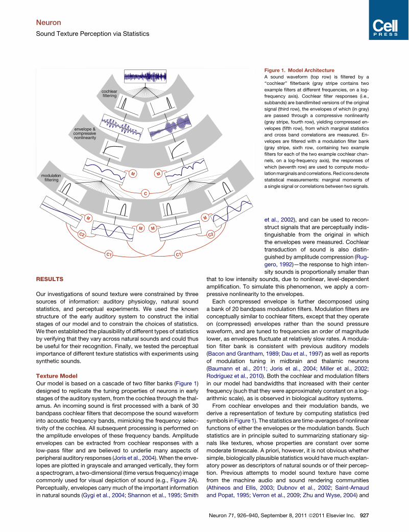
Texture ModelOur model is based on a cascade of two filter banks (Figure 1)designed to replicate the tuning properties of neurons in earlystages of the auditory system, from the cochlea through the thal-amus. An incoming sound is first processed with a bank of 30bandpass cochlear filters that decompose the sound waveforminto acoustic frequency bands, mimicking the frequency selec-tivity of the cochlea. All subsequent processing is performed onthe amplitude envelopes of these frequency bands. Amplitudeenvelopes can be extracted from cochlear responses with alow-pass filter and are believed to underlie many aspects ofperipheral auditory responses (Joris et al., 2004).When the enve-lopes are plotted in grayscale and arranged vertically, they forma spectrogram, a two-dimensional (time versus frequency) imagecommonly used for visual depiction of sound (e.g., Figure 2A).Perceptually, envelopes carry much of the important informationin natural sounds (Gygi et al., 2004; Shannon et al., 1995; Smith

cochlearfiltering

envelope &compressivenonlinearity

modulationfiltering

C2 C2

C1

C

C1

M M

M

M M

M

Figure 1. Model ArchitectureA sound waveform (top row) is filtered by a

‘‘cochlear’’ filterbank (gray stripe contains two

example filters at different frequencies, on a log-

frequency axis). Cochlear filter responses (i.e.,

subbands) are bandlimited versions of the original

signal (third row), the envelopes of which (in gray)

are passed through a compressive nonlinearity

(gray stripe, fourth row), yielding compressed en-

velopes (fifth row), from which marginal statistics

and cross band correlations are measured. En-

velopes are filtered with a modulation filter bank

(gray stripe, sixth row, containing two example

filters for each of the two example cochlear chan-

nels, on a log-frequency axis), the responses of

which (seventh row) are used to compute modu-

lationmarginals andcorrelations.Red iconsdenote

statistical measurements: marginal moments of

a single signal or correlations between two signals.

et al., 2002), and can be used to recon-struct signals that are perceptually indis-tinguishable from the original in whichthe envelopes were measured. Cochleartransduction of sound is also distin-guished by amplitude compression (Rug-gero, 1992)—the response to high inten-sity sounds is proportionally smaller than

that to low intensity sounds, due to nonlinear, level-dependentamplification. To simulate this phenomenon, we apply a com-pressive nonlinearity to the envelopes.Each compressed envelope is further decomposed using

a bank of 20 bandpass modulation filters. Modulation filters areconceptually similar to cochlear filters, except that they operateon (compressed) envelopes rather than the sound pressurewaveform, and are tuned to frequencies an order of magnitudelower, as envelopes fluctuate at relatively slow rates. A modula-tion filter bank is consistent with previous auditory models(Bacon and Grantham, 1989; Dau et al., 1997) as well as reportsof modulation tuning in midbrain and thalamic neurons(Baumann et al., 2011; Joris et al., 2004; Miller et al., 2002;Rodrıguez et al., 2010). Both the cochlear and modulation filtersin our model had bandwidths that increased with their centerfrequency (such that they were approximately constant on a log-arithmic scale), as is observed in biological auditory systems.From cochlear envelopes and their modulation bands, we

derive a representation of texture by computing statistics (redsymbols in Figure 1). The statistics are time-averages of nonlinearfunctions of either the envelopes or the modulation bands. Suchstatistics are in principle suited to summarizing stationary sig-nals like textures, whose properties are constant over somemoderate timescale. A priori, however, it is not obvious whethersimple, biologically plausible statistics would havemuch explan-atory power as descriptors of natural sounds or of their percep-tion. Previous attempts to model sound texture have comefrom the machine audio and sound rendering communities(Athineos and Ellis, 2003; Dubnov et al., 2002; Saint-Arnaudand Popat, 1995; Verron et al., 2009; Zhu and Wyse, 2004) and

Neuron

Sound Texture Perception via Statistics

Neuron 71, 926–940, September 8, 2011 ª2011 Elsevier Inc. 927

have involved representations unrelated to those in biologicalauditory systems.

Texture StatisticsOf all the statistics the brain could compute, whichmight be usedby the auditory system? Natural sounds can provide clues: inorder for a statistic to be useful for recognition, it must producedifferent values for different sounds. We considered a set ofgeneric statistics and verified that they varied substantiallyacross a set of 168 natural sound textures.

We examined two general classes of statistic: marginalmoments and pairwise correlations. Both types of statisticinvolve averages of simple nonlinear operations (e.g., squaring,products) that could plausibly bemeasured using neural circuitryat a later stage of neural processing. Moments and correlationsderive additional plausibility from their importance in the repre-

Cochlear Channel (Hz) 596 2507 8844

596 2507 8844Cochlear Channel (Hz)

Env

elop

e K

urto

sis

Env

elop

e M

ean

Cochlear Channel (Hz)

10

3

20

Env

elop

e Va

rianc

e/M

ean

2

10-2

10-1

10 0

A

D E

B

G

596 2507 88440

.05

.1

.15

.2

.25

0 0.1 0.2 0.3

Pro

b. o

f Occ

urre

nce

Noise

Stream

Geese

Envelope Histograms (2200 Hz Channel)10 0

10-2

10-4

Envelope Magnitude

C

596 2507 8844-2

0

2

4

Cochlear Channel (Hz)

Env

elop

e S

kew

F

0.5 1 1.50

0.1

0.2

0.3

0.4

Pink Noise

Coc

hlea

r C

hann

el (

Hz)

Time (sec)0.5 1.5

8844

2507

596

Stream

Time (sec)0.5 1.5

8844

2507

596

Geese

Time (sec)0.5 1.5

8844

2507

596

Time (sec)

1 1 1

Envelopes (2200 Hz Channel)

52 52 52

52 52

52 52

Figure 2. Cochlear Marginal Statistics(A) Spectrograms of three sound excerpts, gen-

erated by plotting the envelopes of a cochlear filter

decomposition. Gray-level indicates the (com-

pressed) envelope amplitude (same scale for all

three sounds).

(B) Envelopes of one cochlear channel for the

three sounds from (A).

(C) Histograms (gathered over time) of the enve-

lopes in (B). Vertical line segments indicate the

mean value of the envelope for each sound.

(D–G) Envelope marginal moments for each

cochlear channel of each of 168 natural sound

textures. Moments of sounds in (A–C) are plotted

with thick lines; dashed black line plots the mean

value of each moment across all sounds.

sentation of visual texture (Heeger andBergen, 1995; Portilla and Simoncelli,2000), which provided inspiration for ourwork. Both types of statistic werecomputed on cochlear envelopes aswell as their modulation bands (Figure 1).Because modulation filters are applied tothe output of a particular cochlearchannel, they are tuned in both acousticfrequency and modulation frequency.We thus distinguished two types ofmodulation correlations: those betweenbands tuned to the same modulationfrequency but different acoustic frequen-cies (C1), and those between bandstuned to the same acoustic frequencybut different modulation frequencies (C2).

To provide some intuition for thevariation in statistics that occurs acrosssounds, consider the cochlear marginalmoments: statistics that describe thedistribution of the envelope amplitudefor a single cochlear channel. Figure 2Ashows the envelopes, displayed as spec-trograms, for excerpts of three example

sounds (pink [1/f] noise, a stream, andgeese calls), and Figure 2Bplots the envelopes of one particular channel for each sound. It isvisually apparent that the envelopes of the three sounds aredistributed differently—those of the geese contain more high-amplitude and low-amplitude values than those of the streamor noise. Figure 2C shows the envelope distributions for onecochlear channel. Although the mean envelope values are nearlyequal in this example (because they have roughly the sameaverage acoustic power in that channel), the envelope distribu-tions differ in width, asymmetry about the mean, andthe presence of a long positive tail. These properties can becaptured by the marginal moments (mean, variance, skew, andkurtosis, respectively). Figures 2D–2G show these moments forour full set of sound textures. Marginal moments have previouslybeen proposed to play a role in envelope discrimination (Lorenziet al., 1999; Strickland and Viemeister, 1996), and often reflect

Neuron



the property of sparsity, which tends to characterize naturalsounds and images (Field, 1987; Attias and Schreiner, 1998).Intuitively, sparsity reflects the discrete events that generatenatural signals; these events are infrequent, but produce a burstof energy when they occur, yielding high-variance amplitudedistributions. Sparsity has been linked to sensory coding (Field,1987; Olshausen and Field, 1996; Smith and Lewicki, 2006), butits role in the perception of real-world sounds has been unclear.Each of the remaining statistics we explored (Figure 1)

captures distinct aspects of acoustic structure and also exhibitslarge variation across sounds (Figure 3). The moments of themodulation bands, particularly the variance, indicate the ratesat which cochlear envelopes fluctuate, allowing distinctionbetween rapidly modulated sounds (e.g., insect vocalizations)and slowly modulated sounds (e.g., ocean waves). The correla-tion statistics, in contrast, each reflect distinct aspects of coor-

dination between envelopes of different channels, or betweentheir modulation bands. The cochlear correlations (C) distinguishtextures with broadband events that activate many channelssimultaneously (e.g., applause), from those that produce nearlyindependent channel responses (many water sounds; seeExperiment 1: Texture Identification). The cross-channel modu-lation correlations (C1) are conceptually similar except thatthey are computed on a particular modulation band of each co-chlear channel. In some sounds (e.g., wind, or waves) the C1correlations are large only for low modulation-frequency bands,whereas in others (e.g., fire) they are present across all bands.The within-channel modulation correlations (C2) allow discrimi-nation between sounds with sharp onsets or offsets (or both),by capturing the relative phase relationships between modula-tion bands within a cochlear channel. See Experimental Proce-dures for detailed descriptions.

3.13 Hz 3.13 Hz6.25 Hz

12.5 Hz

6.25 Hz

12.5 Hz25 Hz 25 Hz

Waves FireC

WavesInsects Stream

Cochlear Channel (Hz)Modulation Channel (Hz)

StreamApplauseFire

Coc

hlea

r C

hann

el (

Hz)

8844

2507

596

52

Modulation Channel (Hz)Time (s)

Firecrackers

Reverse Snare Drums

Tapping

C2 Real C2 Imag. 1

0

-1

-.5

.5

1

0

-1

A

D

B

200 1.8 8.5 41.3 -15

15

1

0

-1

-.5

.5

88442507 596 52Coc

hlea

r C

hann

el (

Hz)

8844

2507

596

52

Coc

hlea

r C

hann

el (

Hz)

8844

2507

596

52

0

1 2 3 4 5 1.6 25 1.6 25Cochlear Channel (Hz)

88442507 596 52

Coc

hlea

r C

hann

el (

Hz)

8844

2507

596

52

50 Hz 100 Hz 50 Hz 100 Hz

Figure 3. Modulation Power and Correlation Statistics(A) Modulation power in each band (normalized by the variance of the corresponding cochlear envelope) for insects, waves, and stream sounds of Figure 4B. For

ease of display and interpretation, this statistic is expressed in dB relative to the same statistic for pink noise.

(B) Cross-band envelope correlations for fire, applause, and stream sounds of Figure 4B. Each matrix cell displays the correlation coefficient between a pair of

cochlear envelopes.

(C) C1 correlations for waves and fire sounds of Figure 4B. Eachmatrix contains correlations betweenmodulation bands tuned to the samemodulation frequency

but to different acoustic frequencies, yielding matrices of the same format as (B), but with a different matrix for each modulation frequency, indicated at the top of

each matrix.

(D) Spectrograms and C2 correlations for three sounds. Note asymmetric envelope shapes in first and second rows, and that abrupt onsets (top), offsets (middle),

and impulses (bottom) produce distinct correlation patterns. In right panels, modulation channel labels indicate the center of low-frequency band contributing to

the correlation. See also Figure S6.

Neuron



Sound SynthesisOur goal in synthesizing sounds was not to render maximallyrealistic sounds per se, as in most sound synthesis applications(Dubnov et al., 2002; Verron et al., 2009), but rather to testhypotheses about how the brain represents sound texture, usingrealism as an indication of the hypothesis validity. Others havealso noted the utility of synthesis for exploring biological auditoryrepresentations (Mesgarani et al., 2009; Slaney, 1995); our workis distinct for its use of statistical representations. Inspired bymethods for visual texture synthesis (Heeger and Bergen, 1995;Portilla and Simoncelli, 2000), our method produced novelsignals thatmatched some of the statistics of a real-world sound.If the statistics used to synthesize the sound are similar to thoseused by the brain for texture recognition, the synthetic signalshould sound like another example of the original sound.

To synthesize a texture, we first obtained desired values ofthe statistics by measuring the model responses (Figure 1) fora real-world sound. We then used an iterative procedureto modify a random noise signal (using variants of gradientdescent) to force it to have these desired statistic values (Fig-ure 4A). By starting from noise, we hoped to generate a signalthat was as random as possible, constrained only by the desiredstatistics.

Figure 4B displays spectrograms of several naturally occurringsound textures along with synthetic examples generated fromtheir statistics (see Figure S1 available online for additionalexamples). It is visually apparent that the synthetic sounds sharemany structural properties of the originals, but also that the pro-cess has not simply regenerated the original sound—here and inevery other example we examined, the synthetic signals werephysically distinct from the originals (see also Experiment 1:Texture Identification [Experiment 1b, condition 7]). Moreover,running the synthesis procedure multiple times produced exem-plars with the same statistics but whose spectrograms wereeasily discriminated visually (Figure S2). The statistics westudied thus define a large set of sound signals (including theoriginal in which the statistics are measured), from which onemember is drawn each time the synthesis process is run.

To assess whether the synthetic results sound like the naturaltextures whose statistics they matched, we conducted severalexperiments. The results can also be appreciated by listeningto example synthetic sounds, available online (http://www.cns.nyu.edu/!lcv/sound_texture.html).

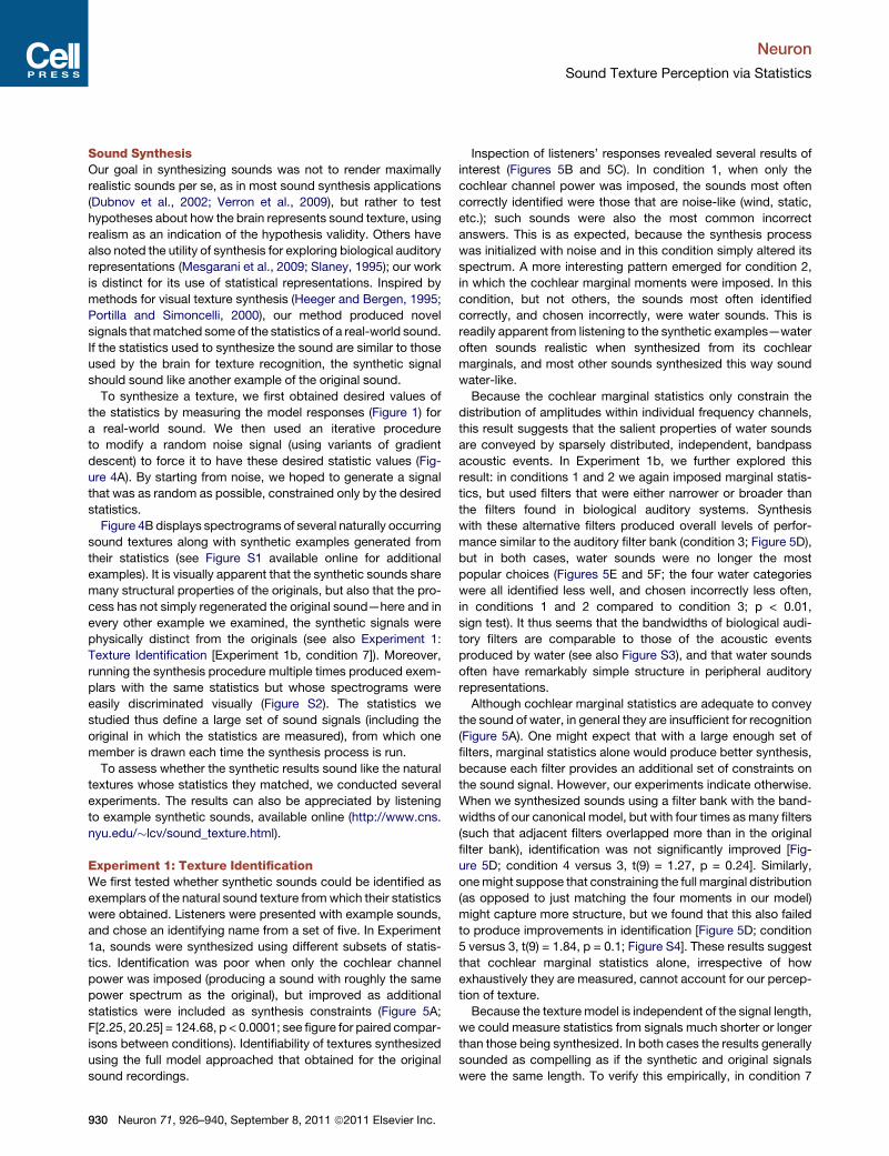
Experiment 1: Texture IdentificationWe first tested whether synthetic sounds could be identified asexemplars of the natural sound texture fromwhich their statisticswere obtained. Listeners were presented with example sounds,and chose an identifying name from a set of five. In Experiment1a, sounds were synthesized using different subsets of statis-tics. Identification was poor when only the cochlear channelpower was imposed (producing a sound with roughly the samepower spectrum as the original), but improved as additionalstatistics were included as synthesis constraints (Figure 5A;F[2.25, 20.25] = 124.68, p < 0.0001; see figure for paired compar-isons between conditions). Identifiability of textures synthesizedusing the full model approached that obtained for the originalsound recordings.

Inspection of listeners’ responses revealed several results ofinterest (Figures 5B and 5C). In condition 1, when only thecochlear channel power was imposed, the sounds most oftencorrectly identified were those that are noise-like (wind, static,etc.); such sounds were also the most common incorrectanswers. This is as expected, because the synthesis processwas initialized with noise and in this condition simply altered itsspectrum. A more interesting pattern emerged for condition 2,in which the cochlear marginal moments were imposed. In thiscondition, but not others, the sounds most often identifiedcorrectly, and chosen incorrectly, were water sounds. This isreadily apparent from listening to the synthetic examples—wateroften sounds realistic when synthesized from its cochlearmarginals, and most other sounds synthesized this way soundwater-like.Because the cochlear marginal statistics only constrain the

distribution of amplitudes within individual frequency channels,this result suggests that the salient properties of water soundsare conveyed by sparsely distributed, independent, bandpassacoustic events. In Experiment 1b, we further explored thisresult: in conditions 1 and 2 we again imposed marginal statis-tics, but used filters that were either narrower or broader thanthe filters found in biological auditory systems. Synthesiswith these alternative filters produced overall levels of perfor-mance similar to the auditory filter bank (condition 3; Figure 5D),but in both cases, water sounds were no longer the mostpopular choices (Figures 5E and 5F; the four water categorieswere all identified less well, and chosen incorrectly less often,in conditions 1 and 2 compared to condition 3; p < 0.01,sign test). It thus seems that the bandwidths of biological audi-tory filters are comparable to those of the acoustic eventsproduced by water (see also Figure S3), and that water soundsoften have remarkably simple structure in peripheral auditoryrepresentations.Although cochlear marginal statistics are adequate to convey

the sound of water, in general they are insufficient for recognition(Figure 5A). One might expect that with a large enough set offilters, marginal statistics alone would produce better synthesis,because each filter provides an additional set of constraints onthe sound signal. However, our experiments indicate otherwise.When we synthesized sounds using a filter bank with the band-widths of our canonical model, but with four times asmany filters(such that adjacent filters overlapped more than in the originalfilter bank), identification was not significantly improved [Fig-ure 5D; condition 4 versus 3, t(9) = 1.27, p = 0.24]. Similarly,onemight suppose that constraining the full marginal distribution(as opposed to just matching the four moments in our model)might capture more structure, but we found that this also failedto produce improvements in identification [Figure 5D; condition5 versus 3, t(9) = 1.84, p = 0.1; Figure S4]. These results suggestthat cochlear marginal statistics alone, irrespective of howexhaustively they are measured, cannot account for our percep-tion of texture.Because the texture model is independent of the signal length,

we could measure statistics from signals much shorter or longerthan those being synthesized. In both cases the results generallysounded as compelling as if the synthetic and original signalswere the same length. To verify this empirically, in condition 7

Neuron



http://www.cns.nyu.edu/~lcv/sound_texture.html



we used excerpts of 15 s signals synthesized from 7 s originals.Identification performance was unaffected [Figure 5D; condition7 versus 6; t(9) = 0.5, p = 0.63], indicating that these longersignals captured the texture qualities as well as signals morecomparable to the original signals in length.

Experiment 2: Necessity of Each Class of StatisticWe found that each class of statistic was perceptually neces-sary, in that its omission from the model audibly impaired thequality of some synthetic sounds. To demonstrate this empiri-cally, in Experiment 2a we presented listeners with excerpts

A

Coc

hlea

r C

hann

el (

Hz)

8844

2507

596

52

8844

2507

596

52

8844

2507

596

52

8844

2507

596

52

8844

2507

596

52

8844

2507

596

52

Stream Geese

Fire Applause

Insects Waves

ORIGINAL SYNTHETIC ORIGINAL SYNTHETICB

Time (sec) Time (sec)

1 2 3 4 1 2 3 4 1 2 3 4 1 2 3 4

whitenoise

originalsound

!ne structure

Analysis

Synthesis

measurestatistics

measurestatistics

measurestatistics

measurestatistics

modulationfiltering

extractenvelope

extractenvelope

cochlearfiltering

cochlearfiltering

imposestatistics

combinesubbands

syntheticsound

modulationfiltering

÷

x

Figure 4. Synthesis Algorithm and Example Results(A) Schematic of synthesis procedure. Statistics are measured after a sound recording is passed through the auditory model of Figure 1. Synthetic signal is

initialized as noise, and the original sound’s statistics are imposed on its cochlear envelopes. The modified envelopes are multiplied by their associated fine

structure, and then recombined into a sound signal. The procedure is iterated until the synthesized signal has the desired statistics.

(B) Spectrograms of original and synthetic versions of several sounds (same amplitude scale for all sounds). See also Figure S1 and Figure S2.

Neuron



of original texture recordings followed by two syntheticversions—one synthesized using the full set of model statistics,and the other synthesized with one class omitted—and askedthem to judge which synthetic version sounded more like theoriginal. Figure 6A plots the percentage of trials on which thefull set of statistics was preferred. In every condition, thispercentage was greater than that expected by chance (t tests,p < 0.01 in all cases, Bonferroni corrected), though the prefer-ence was stronger for some statistic classes than others[F(4,36) = 15.39, p < 0.0001].

The effect of omitting a statistic class was not noticeable forevery texture. A potential explanation is that the statistics ofmany textures are close to those of noise for some subset ofstatistics, such that omitting that subset does not cause thestatistics of the synthetic result to deviate much from the correct

values (because the synthesis is initialized with noise). To testthis idea, we computed the difference between each sound’sstatistics and those of pink (1/f) noise, for each of the five statisticclasses. When we reanalyzed the data including only the 30% ofsounds whose statistics were most different from those of noise,the proportion of trials on which the full set of statistics waspreferred was significantly higher in each case (t tests, p <0.05). Including a particular statistic in the synthesis processthus tends to improve realism when the value of that statisticdeviates from that of noise. Because of this, not all statisticsare necessary for the synthesis of every texture (although allstatistics presumably contribute to the perception of everytexture—if the values were actively perturbed from their correctvalues, whether noise-like or not, we found that listeners gener-ally noticed).

0

20

40

60

80

100

Wind (88)Radio Static (85)Bees (80)Rain (72)Vacuum Cleaner (70)

Water in Sink (100)Bees (95)Bubbling Water (95)River (93)Rain (92)

Wind (52)Radio Static (49)Rain (46)Bees (39)Vacuum Cleaner (38)

River (70)Bubbling Water (70)Rain (54)Water in Sink (54)Insects (26)

A D

Applause (85)Radio Static (80)Bubbling Water (80)Train (77)Wind (72)

Fire Alarm Bell (100)Gargling (90)Bees (90)Babble (85)Insects (85)

Water in Sink (51)Radio Static (37)Rain (36)Bubbling Water (32)Applause (30)

Babble (36)Bees (35)Vacuum Cleaner (31)Noisy Machinery (27)Birds (23)

Bubbling Water (100)Bees (95)Gargling (90)River (82)Water in Sink (80)

Water in Sink (78)Bubbling Water (62)River (54)Rain (37)Gargling (33)

Per

cent

Cor

rect

0

20

40

60

80

100

Per

cent

Cor

rect

1) P

ower

only

2) M

argin

als o

nly

3) M

argin

als +

Coc

h. C

orr.

(C)

4) M

arg.

+ M

odula

tion

power

5) M

arg.

+ C

+ M

od. p

ower

6) M

arg.

+ C

+ M

od. p

ower

+ C

1

8) M

arg.

+ C

+ M

od. p

ower

+ C

1 +

C2

9) O

rigina

l sou

nds

1) M

argin

als -

Broad

filte

rs

2) M

argin

als -

Narro

w filte

rs

3) M

argin

als -

Cochle

ar fil

ters

4) M

argin

als -

Cochle

ar fil

ters

, 4x

5) M

argin

als (f

ull h

ist.)

- Coc

hlear

filte

rs

6) A

ll sta

ts - C

ochle

ar fil

ters

7) A

ll sta

ts - C

ochle

ar fil

ters

, Lon

g sy

nth.

B

C

E

F

7) M

arg.

+ C

+ M

od. p

ower

+ C

2

*

** * *

n.s.n.s.

n.s.

Figure 5. Experiment 1: Texture Identification(A) Identification improves as more statistics are included in the synthesis. Asterisks denote significant differences between conditions, p < 0.01 (paired t tests,

corrected for multiple comparisons). Here and elsewhere, error bars denote standard errors and dashed lines denote the chance level of performance.

(B) The five categories correctly identified most often for conditions 1 and 2, with mean percent correct in parentheses.

(C) The five categories chosen incorrectly most often for conditions 1 and 2, with mean percent trials chosen (of those where they were a choice) in parentheses.

(D) Identification with alternative marginal statistics, and long synthetic signals. Horizontal lines indicate nonsignificant differences (p > 0.05).

(E and F) The five (E) most correctly identified and (F) most often incorrectly chosen categories for conditions 1–3. See also Figure S3 and Figure S4.

Neuron



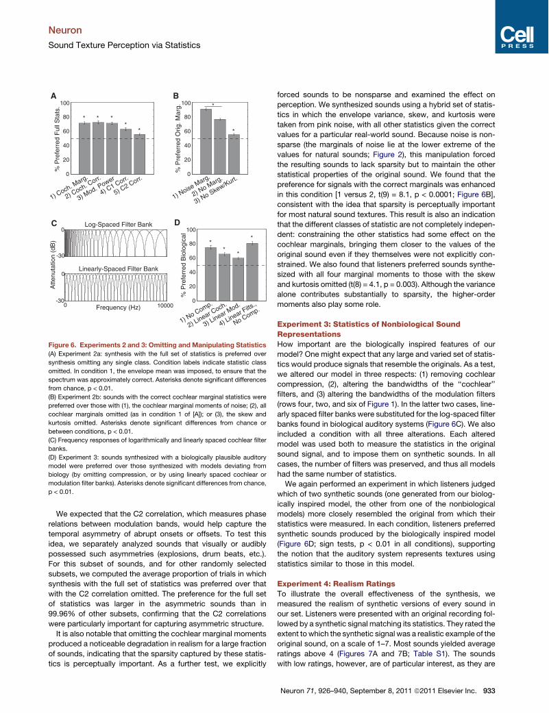
We expected that the C2 correlation, which measures phaserelations between modulation bands, would help capture thetemporal asymmetry of abrupt onsets or offsets. To test thisidea, we separately analyzed sounds that visually or audiblypossessed such asymmetries (explosions, drum beats, etc.).For this subset of sounds, and for other randomly selectedsubsets, we computed the average proportion of trials in whichsynthesis with the full set of statistics was preferred over thatwith the C2 correlation omitted. The preference for the full setof statistics was larger in the asymmetric sounds than in99.96% of other subsets, confirming that the C2 correlationswere particularly important for capturing asymmetric structure.It is also notable that omitting the cochlear marginal moments

produced a noticeable degradation in realism for a large fractionof sounds, indicating that the sparsity captured by these statis-tics is perceptually important. As a further test, we explicitly

forced sounds to be nonsparse and examined the effect onperception. We synthesized sounds using a hybrid set of statis-tics in which the envelope variance, skew, and kurtosis weretaken from pink noise, with all other statistics given the correctvalues for a particular real-world sound. Because noise is non-sparse (the marginals of noise lie at the lower extreme of thevalues for natural sounds; Figure 2), this manipulation forcedthe resulting sounds to lack sparsity but to maintain the otherstatistical properties of the original sound. We found that thepreference for signals with the correct marginals was enhancedin this condition [1 versus 2, t(9) = 8.1, p < 0.0001; Figure 6B],consistent with the idea that sparsity is perceptually importantfor most natural sound textures. This result is also an indicationthat the different classes of statistic are not completely indepen-dent: constraining the other statistics had some effect on thecochlear marginals, bringing them closer to the values of theoriginal sound even if they themselves were not explicitly con-strained. We also found that listeners preferred sounds synthe-sized with all four marginal moments to those with the skewand kurtosis omitted (t(8) = 4.1, p = 0.003). Although the variancealone contributes substantially to sparsity, the higher-ordermoments also play some role.

Experiment 3: Statistics of Nonbiological SoundRepresentationsHow important are the biologically inspired features of ourmodel? One might expect that any large and varied set of statis-tics would produce signals that resemble the originals. As a test,we altered our model in three respects: (1) removing cochlearcompression, (2), altering the bandwidths of the ‘‘cochlear’’filters, and (3) altering the bandwidths of the modulation filters(rows four, two, and six of Figure 1). In the latter two cases, line-arly spaced filter banks were substituted for the log-spaced filterbanks found in biological auditory systems (Figure 6C). We alsoincluded a condition with all three alterations. Each alteredmodel was used both to measure the statistics in the originalsound signal, and to impose them on synthetic sounds. In allcases, the number of filters was preserved, and thus all modelshad the same number of statistics.We again performed an experiment in which listeners judged

which of two synthetic sounds (one generated from our biolog-ically inspired model, the other from one of the nonbiologicalmodels) more closely resembled the original from which theirstatistics were measured. In each condition, listeners preferredsynthetic sounds produced by the biologically inspired model(Figure 6D; sign tests, p < 0.01 in all conditions), supportingthe notion that the auditory system represents textures usingstatistics similar to those in this model.

Experiment 4: Realism RatingsTo illustrate the overall effectiveness of the synthesis, wemeasured the realism of synthetic versions of every sound inour set. Listeners were presented with an original recording fol-lowed by a synthetic signal matching its statistics. They rated theextent to which the synthetic signal was a realistic example of theoriginal sound, on a scale of 1–7. Most sounds yielded averageratings above 4 (Figures 7A and 7B; Table S1). The soundswith low ratings, however, are of particular interest, as they are

0

20

40

60

80

100

5) C2 Corr.

* * **

*

% P

refe

rred

Ful

l Sta

ts.

4) C1 Corr.

3) Mod. P

ower

1) Coch. M

arg.

2) Coch. C

orr.0

20

40

60

80

100

% P

refe

rred

Orig

. Mar

g.

3) No Skew/Kurt.

2) No Marg.

1) Noise Marg.

*

*

BA

0

20

40

60

80

100

% P

refe

rred

Bio

logi

cal

3) Linear Mod.

1) No Comp.

2) Linear Coch.

D

**

*

*

Log-Spaced Filter Bank

Linearly-Spaced Filter Bank

Atte

nuta

tion

(dB

)

C

Frequency (Hz)0 10000-30

0

-30

0

4) Linear Filts.,

No Comp.

Figure 6. Experiments 2 and 3: Omitting and Manipulating Statistics(A) Experiment 2a: synthesis with the full set of statistics is preferred over

synthesis omitting any single class. Condition labels indicate statistic class

omitted. In condition 1, the envelope mean was imposed, to ensure that the

spectrum was approximately correct. Asterisks denote significant differences

from chance, p < 0.01.

(B) Experiment 2b: sounds with the correct cochlear marginal statistics were

preferred over those with (1), the cochlear marginal moments of noise; (2), all

cochlear marginals omitted (as in condition 1 of [A]); or (3), the skew and

kurtosis omitted. Asterisks denote significant differences from chance or

between conditions, p < 0.01.

(C) Frequency responses of logarithmically and linearly spaced cochlear filter

banks.

(D) Experiment 3: sounds synthesized with a biologically plausible auditory

model were preferred over those synthesized with models deviating from

biology (by omitting compression, or by using linearly spaced cochlear or

modulation filter banks). Asterisks denote significant differences from chance,

p < 0.01.

Neuron



statistically matched to the original recordings and yet do notsound like them. Figure 7C lists the sounds with average ratingsbelow 2. They fall into three general classes—those involvingpitch (railroad crossing, wind chimes, music, speech, bells),rhythm (tapping, music, drumming), and reverberation (drumbeats, firecrackers); see also Figure S5. This suggests that theperception of these sound attributes involves measurementssubstantially different from those in our model.

DISCUSSION

We have studied ‘‘sound textures,’’ a class of sounds producedby multiple superimposed acoustic events, as are common tomany natural environments. Sound textures are distinguishedby temporal homogeneity, and we propose that they are re-presented in the auditory system with time-averaged statistics.We embody this hypothesis in a model based on statistics(moments and correlations) of a sound decomposition like thatfound in the subcortical auditory system. To test the role of thesestatistics in texture recognition, we conducted experiments withsynthetic sounds matching the statistics of various real-worldtextures. We found that (1) such synthetic sounds could be accu-rately recognized, andat levels far better than if only the spectrumor sparsity was matched, (2) eliminating subsets of the statisticsin themodel reduced the realismof the synthetic results, (3)modi-fying the model to less faithfully mimic the mammalian auditorysystem also reduced the realism of the synthetic sounds, and(4) the synthetic results were often realistic, but failed markedlyfor a few particular sound classes.

Our results suggest that when listeners recognize the soundof rain, fire, insects, and other such sounds, they are recog-nizing statistics of modest complexity computed from theoutput of the peripheral auditory system. These statistics arelikely measured at downstream stages of neural processing,and thus provide clues to the nature of mid-level auditorycomputations.

Neural ImplementationBecause texture statistics are time averages, their computationcan be thought of as involving two steps: a nonlinear functionapplied to the relevant auditory response(s), followed by anaverage over time. A moment, for instance, could be computedby a neuron that averages its input (e.g., a cochlear envelope)after raising it to a power (two for the variance, three for theskew, etc.). We found that envelope moments were crucial forproducing naturalistic synthetic sounds. Envelope momentsconvey sparsity, a quality long known to differentiate naturalsignals from noise (Field, 1987) and one that is central to manyrecent signal-processing algorithms (Asari et al., 2006; Bell andSejnowski, 1996). Our results thus suggest that sparsity is repre-sented in the auditory system and used to distinguish sounds.Although definitive characterization of the neural locus awaits,neural responses in the midbrain often adapt to particular ampli-tude distributions (Dean et al., 2005; Kvale and Schreiner, 2004),raising the possibility that envelope moments may be computedsubcortically. Themodulation power (also amarginal moment) atparticular rates also seems to be reflected in the tuning of manythalamic and midbrain neurons (Joris et al., 2004).The other statistics in our model are correlations. A correlation

is the average of a normalized product (e.g., of two cochlearenvelopes), and could be computed as such. However, a correla-tion can also be viewed as the proportion of variance in one vari-able that is shared by another, which is partly reflected in the vari-ance of the sum of the variables. This formulation provides analternative implementation (see Experimental Procedures), andillustrates that correlations in one stage of representation (e.g.,bandpass cochlear channels) can be reflected in the marginalstatistics of the next (e.g., cortical neurons that sum input frommultiple channels), assuming appropriate convergence. All ofthe texture statistics we have considered could thus reduce tomarginal statistics at different stages of the auditory system.Neuronal tuning to texture statistics could be probed using

synthetic stimuli whose statistics are parametrically varied.

A CB

Average Realism Rating

Num

ber

of S

ound

s

1 2 3 4 5 6 70

10

20

30 Synthetic sounds with lowest realism ratings

1.931.901.771.771.701.701.671.631.601.601.501.501.471.401.371.20

Railroad crossingTapping rhythm - quarter note pairsWind chimesCorkscrew scraping desk edgeReverse snare drum beatsTapping rhythm - quarter note tripletsSnare drum beatsWalking on gravelSnare drum rimshot sequenceMusic - drum breakMusic - mamboBongo drum loopFirecracker explosionsPerson speaking FrenchChurch bellsPerson speaking English

Synthetic sounds with high realism ratings

6.576.576.536.476.436.436.406.376.336.206.176.136.005.905.905.875.875.705.675.67

Insects in swampHeavy rain on hard surfaceFrogsApplause - big roomRadio staticStreamAir conditionerFrying eggsWind blowingSparrows - large excited groupJackhammerWater trickling into poolFire - forest infernoBee swarmRustling paperTrain speeding down tracksRattlesnake rattleCocktail party babbleShaking coinsHelicopter

Figure 7. Experiment 4: Realism Ratings(A) Histogram of average realism ratings for each sound in our set.

(B) List of 20 sound textures with high average ratings. Multiple examples of similar sounds are omitted for brevity.

(C) List of all sounds with average realism ratings <2, along with their average rating. See Table S1 for complete list. See also Figure S5.

Neuron



Stationary artificial sounds have a long history of use in psycho-acoustics and neurophysiology, with recent efforts to incorpo-rate naturalistic statistical structure (Attias and Schreiner,1998; Garcia-Lazaro et al., 2006; McDermott et al., 2011; Over-ath et al., 2008; Rieke et al., 1995; Singh and Theunissen, 2003).Stimuli synthesized from our model capture naturally occurringsound structure while being precisely characterized within anauditory model. They offer a middle ground between naturalsounds and the tones and noises of classical hearing research.

Relation to Visual TextureVisual textures, unlike their auditory counterparts, have beenstudied intensively for decades (Julesz, 1962), and our workwas inspired by efforts to understand visual texture usingsynthesis (Heeger and Bergen, 1995; Portilla and Simoncelli,2000; Zhu et al., 1997). How similar are visual and auditorytexture representations? For ease of comparison, Figure 8shows amodel diagram of the most closely related visual texturemodel (Portilla and Simoncelli, 2000), analogous in format to ourauditory model (Figure 1) but with input signals and representa-tional stages that vary spatially rather than temporally. The visionmodel has two stages of linear filtering (corresponding to LGNcells and V1 simple cells) followed by envelope extraction (corre-sponding to V1 complex cells), whereas the auditory model hasthe envelope operation sandwiched between linear filteringoperations (corresponding to the cochlea and midbrain/thal-amus), reflecting structural differences in the two systems. Thereare also notable differences in the stages at which statistics arecomputed in the two models: several types of visual texturestatistics are computed directly on the initial linear filteringstages, whereas the auditory statistics all follow the envelope

Figure 8. Analogous Model of VisualTexture RepresentationModel is depicted in a format like that of the

auditory texture model in Figure 1. An image of

beans (top row) is filtered into spatial frequency

bands by center-surround filters (second row), as

happens in the retina/LGN. The spatial frequency

bands (third row) are filtered again by orientation

selective filters (fourth row) analogous to V1 simple

cells, yielding scale and orientation filtered bands

(fifth row). The envelopes of these bands are ex-

tracted (sixth row) to produce analogs of V1

complex cell responses (seventh row). The linear

function at the envelope extraction stage indicates

the absence of the compressive nonlinearity

present in the auditory model. As in Figure 1, red

icons denote statistical measurements: marginal

moments of a single signal (M) or correlations

between two signals (AC, C1, or C2 for autocor-

relation, cross-band correlation, or phase-

adjusted correlation). C1 and C2 here and in Fig-

ure 1 denote conceptually similar statistics. The

autocorrelation (AC) is identical to C1 except that it

is computed within a channel. This model is

a variant of Portilla and Simoncelli (2000).

operation, reflecting the primary locus ofstructure in images versus sounds.However, the statistical computations

themselves—marginal moments and correlations—are concep-tually similar in the twomodels. In both systems, relatively simplestatistics capture texture structure, suggesting that textureperception, like filling in (McDermott and Oxenham, 2008;Warren et al., 1972), and saliency (Cusack and Carlyon, 2003;Kayser et al., 2005), may involve analogous computations acrossmodalities.It will be interesting to explore whether the similarities between

modalities extend to inattention, to which visual texture isbelieved to be robust (Julesz, 1962). Under conditions of focusedlistening, we are often aware of individual events composing asound texture, presumably in addition to registering time-aver-aged statistics that characterize the texture qualities. A classicexample is the ‘‘cocktail party problem,’’ in which we attend toa single person talking in a room dense with conversations (Beeand Micheyl, 2008; McDermott, 2009). Without attention, indi-vidual voices or other sound sources are likely inaccessible, butwe may retain access to texture statistics that characterize thecombined effect of multiple sources, as is apparently the casein vision (Alvarez andOliva, 2009). This possibility could be testedin divided attention experiments with synthetic textures.

Texture ExtensionsWe explored the biological representation of sound texture usinga set of generic statistics and a relatively simple auditory model,both of which could be augmented in interesting ways. The threesources of information that contributed to the present work—auditory neuroscience, natural sound analysis, and perceptualexperiments—all provide directions for such extensions.The auditory model of Figure 1, from which statistics are com-

puted, captures neuronal tuning characteristics of subcortical

Neuron



structures. Incorporating cortical tuning properties would likelyextend the range of textures we can account for. For instance,cortical receptive fields have spectral tuning that is morecomplex and varied than that found subcortically (Barbour andWang, 2003; Depireux et al., 2001), and statistics of filtersmodeled on their properties could capture higher-order structurethat our current model does not. As discussed earlier, the cor-relations computed on subcortical representations could thenpotentially be replaced by marginal statistics of filters at a laterstage.

It may also be possible to derive additional or alternativetexture statistics from an analysis of natural sounds, similar inspirit to previous derivations of cochlear and V1 filters fromnatural sounds and images (Olshausen and Field, 1996; Smithand Lewicki, 2006), and consistent with other examples of con-gruence between properties of perceptual systems and naturalenvironments (Attias and Schreiner, 1998; Garcia-Lazaro et al.,2006; Lesica and Grothe, 2008; Nelken et al., 1999; Riekeet al., 1995; Rodrıguez et al., 2010; Schwartz and Simoncelli,2001; Woolley et al., 2005). We envision searching for statisticsthat vary maximally across sounds and would thus be optimalfor recognition.

The sound classes for which the model failed to pro-duce convincing synthetic examples (revealed by Experiment4) also provide directions for exploration. Notable failures includetextures involving pitched sounds, reverberation, and rhythmicstructure (Figure 7, Table S1, and Figure S5). It was not obviousa priori that these sounds would produce synthesis failures—they each contain spectral and temporal structures that arestationary (given a moderately long time window), and we antic-ipated that they might be adequately constrained by the modelstatistics. However, our results show that this is not the case,suggesting that the brain is measuring something that the modelis not.

Rhythmic structure might be captured with another stage ofenvelope extraction and filtering, applied to the modulationbands. Such filters would measure ‘‘second-order’’ modulationof modulation (Lorenzi et al., 2001), as is common in rhythmicsounds. Alternatively, rhythm could involve a measure specifi-cally of periodic modulation patterns. Pitch and reverberationmay also implicate dedicated mechanisms. Pitch is largelyconveyed by harmonically related frequencies, which are notmade explicit by the pair-wise correlations across frequencyfound in our current model (see also Figure S5). Accounting forpitch is thus likely to require a measure of local harmonic struc-ture (de Cheveigne, 2004). Reverberation is also well understoodfrom a physical generative standpoint, as linear filtering of asound source by the environment (Gardner, 1998), and is usedto judge source distance (Zahorik, 2002) and environment prop-erties. However, a listener has access only to the result of envi-ronmental filtering, not to the source or the filter, implying thatreverberation must be reflected in something measured fromthe sound signal (i.e., a statistic). Our synthesis method providesan unexplored avenue for testing theories of the perception ofthese sound properties.

One other class of failures involved mixtures of two soundsthat overlap in peripheral channels but are acoustically distinct,such as broadband clicks and slow bandpass modulations.

These failures likely result because the model statistics are aver-ages over time, and combine measurements that should besegregated. This suggests a more sophisticated form of esti-mating statistics, in which averaging is performed after (or inalternation with) some sort of clustering operation, a key ingre-dient in recent models of stream segregation (Elhilali andShamma, 2008).

Using Texture to Understand RecognitionRecognition is challenging because the sensory input arisingfrom different exemplars of a particular category in the worldoften varies substantially. Perceptual systems must processtheir input to obtain representations that are invariant to the vari-ation within categories, while maintaining selectivity betweencategories (DiCarlo and Cox, 2007). Our texture model incorpo-rates an explicit form of invariance by representing all possibleexemplars of a given texture (Figure S2) with a single set ofstatistic values. Moreover, different textures produce differentstatistics, providing an implicit form of selectivity. However, ourmodel captures texture properties with a large number of simplestatistics that are partially redundant. Humans, in contrast, cate-gorize sounds into semantic classes, and seem to haveconscious access to a fairly small set of perceptual dimensions.It should be possible to learn such lower-dimensional represen-tations of categories from our sound statistics, combining thefull set of statistics into a small number of ‘‘metastatistics’’ thatrelate to perceptual dimensions. We have found, for instance,that most of the variance in statistics over our collection ofsounds can be captured with a moderate number of their prin-cipal components, indicating that dimensionality reduction isfeasible.The temporal averaging through which our texture statistics

achieve invariance is appropriate for stationary sounds, and itis worth considering how this might be relaxed to representsounds that are less homogeneous. A simple possibility involvesreplacing the global time-averages with averages taken overa succession of short timewindows. The resulting local statisticalmeasures would preserve some of the invariance of the globalstatistics, but would follow a trajectory over time, allowing repre-sentation of the temporal evolution of a signal. By computingmeasurements averaged within windows of many durations,the auditory system could derive representations with varyingdegrees of selectivity and invariance, enabling the recognitionof sounds spanning a continuum from homogeneous texturesto singular events.

EXPERIMENTAL PROCEDURES

Auditory ModelOur synthesis algorithm utilized a classic ‘‘subband’’ decomposition in which

a bank of cochlear filters were applied to a sound signal, splitting it into

frequency channels. To simplify implementation, we used zero-phase filters,

with Fourier amplitude shaped as the positive portion of a cosine function.

We used a bank of 30 such filters, with center frequencies equally spaced

on an equivalent rectangular bandwidth (ERB)N scale (Glasberg and Moore,

1990), spanning 52–8844 Hz. Their (3 dB) bandwidths were comparable to

those of the human ear (!5% larger than ERBsmeasured at 55 dB sound pres-

sure level (SPL); we presented sounds at 70 dB SPL, at which human auditory

filters are somewhat wider). The filters did not replicate all aspects of biological

Neuron



auditory filters, but perfectly tiled the frequency spectrum—the summed

squared frequency response of the filter bank was constant across frequency

(to achieve this, the filter bank also included lowpass and highpass filters at the

endpoints of the spectrum). The filter bank thus had the advantage of being

invertible: each subband could be filtered again with the corresponding filter,

and the results summed to reconstruct the original signal (as is standard in

analysis-synthesis subband decompositions [Crochiere et al., 1976]).

The envelope of each subband was computed as the magnitude of its

analytic signal, and the subband was divided by the envelope to yield the

fine structure. The fine structure was ignored for the purposes of analysis

(measuring statistics). Subband envelopes were raised to a power of 0.3 to

simulate basilar membrane compression. For computational efficiency, statis-

tics were measured and imposed on envelopes downsampled (following low-

pass filtering) to a rate of 400 Hz. Although the envelopes of the high-frequency

subbands contained modulations at frequencies above 200 Hz (because

cochlear filters are broad at high frequencies), these were generally low in

amplitude. In pilot experiments we found that using a higher envelope sam-

pling rate did not produce noticeably better synthetic results, suggesting the

high frequency modulations are not of great perceptual significance in this

context.

The filters used to measure modulation power also had half-cosine fre-

quency responses, with center frequencies equally spaced on a log scale

(20 filters spanning 0.5–200 Hz), and a quality factor of 2 (for 3 dB bandwidths),

consistent with those in previous models of human modulation filtering (Dau

et al., 1997), and broadly consistent with animal neurophysiology data (Miller

et al., 2002; Rodrıguez et al., 2010). Although auditory neurons often exhibit

a degree of tuning to spectral modulation as well (Depireux et al., 2001; Rodrı-

guez et al., 2010; Schonwiesner and Zatorre, 2009), this is typically less pro-

nounced than their temporal modulation tuning, particularly early in the audi-

tory system (Miller et al., 2002), and we elected not to include it in our

model. Because 200Hzwas the Nyquist frequency, the highest frequency filter

consisted only of the lower half of the half-cosine frequency response.

We used a smaller set of modulation filters to compute the C1 and C2

correlations, in part because it was desirable to avoid large numbers of unnec-

essary statistics, and in part because the C2 correlations necessitated octave-

spaced filters (see below). These filters also had frequency responses that

were half-cosines on a log-scale, but were more broadly tuned (Q=!!!2

p),

with center frequencies in octave steps from 1.5625 to 100 Hz, yielding seven

filters.

Boundary HandlingAll filtering was performed in the discrete frequency domain, and thus

assumed circular boundary conditions. To avoid boundary artifacts, the statis-

tics measured in original recordings were computed as weighted time-aver-

ages. The weighting window fell from one to zero (half cycle of a raised cosine)

over the 1 s intervals at the beginning and end of the signal (typically a 7 s

segment), minimizing artifactual interactions. For the synthesis process, statis-

tics were imposed with a uniform window, so that they would influence the

entire signal. As a result, continuity was imposed between the beginning and

end of the signal. This was not obvious from listening to the signal once, but

it enabled synthesized signals to be played in a continuous loop without

discontinuities.

StatisticsWe denote the kth cochlear subband envelope by sk(t), and the windowing

function by w(t), with the constraint thatP

t w"t#= 1. The nth modulation

band of cochlear envelope sk is denoted by bk,n(t), computed via convolution

with filter fn.

Cochlear Marginal Statistics

Our texture representation includes the first four normalized moments of the

envelope:

M1k =mk =X

t

w"t#sk"t#;

M2k =s2k

m2k

=

Pt w"t#"sk"t# $ mk#

2

m2k

;

M3k =

Pt w"t#"sk"t# $ mk#

3

s3k

;

and

M4k =

Pt w"t#"sk"t# $ mk#

4

s4k

k˛%1.32& in each case:

The variance was normalized by the squared mean, so as to make it dimen-

sionless like the skew and kurtosis.

The envelope variance, skew, and kurtosis reflect subband sparsity. Spar-

sity is often associated with the kurtosis of a subband (Field, 1987), and prelim-

inary versions of our model were also based on this measurement (McDermott

et al., 2009). However, the envelope’s importance in hearing made its

moments a more sensible choice, and we found them to capture similar spar-

sity behavior.

Figures 2D–2G show the marginal moments for each cochlear envelope of

each sound in our ensemble. All four statistics vary considerably across natural

sound textures. Their values for noise are also informative. The envelope

means, which provide a coarse measure of the power spectrum, do not

have exceptional values for noise, lying in the middle of the set of natural

sounds. However, the remaining envelope moments for noise all lie near the

lower bound of the values obtained for natural textures, indicating that natural

sounds tend to be sparser than noise (see also Experiment 2b) (Attias and

Schreiner, 1998).

Cochlear Cross-Band Envelope Correlation

Cjk =X

t

w"t#"sj"t# $ mj

#"sk"t# $ mk#

sjsk; j; k˛%1.32&

such that "k $ j#˛%1; 2; 3;5; 8; 11; 16; 21&:

Our model included the correlation of each cochlear subband envelope with

a subset of eight of its neighbors, a number that was typically sufficient to

reproduce the qualitative form of the full correlation matrix (interactions

between overlapping subsets of filters allow the correlations to propagate

across subbands). This was also perceptually sufficient: we found informally

that imposing fewer correlations sometimes produced perceptually weaker

synthetic examples, and that incorporating additional correlations did not

noticeably improve the results.

Figure 3B shows the cochlear correlations for recordings of fire, applause,

and a stream. The broadband events present in fire and applause, visible as

vertical streaks in the spectrograms of Figure 4B, produce correlations

between the envelopes of different cochlear subbands. Cross-band correla-

tion, or ‘‘comodulation,’’ is common in natural sounds (Nelken et al., 1999),

and we found it to be to be a major source of variation among sound textures.

The stream, for instance, contains much weaker comodulation.

The mathematical form of the correlation does not uniquely specify the

neural instantiation. It could be computed directly, by averaging a product

as in the above equation. Alternatively, it could be computed with squared

sums and differences, as are common in functional models of neural compu-

tation (Adelson and Bergen, 1985):

Cjk =X

t

w"t#"sj"t# $ mj + sk"t# $ mk

#2$"sj"t# $ mj $ sk"t#+mk

#2

4sjsk:

Modulation Power

For the modulation bands, the variance (power) was the principal marginal

moment of interest. Collectively, these variances indicate the frequencies

present in an envelope. Analogous quantities appear to be represented by

the modulation-tuned neurons common to the early auditory system (whose

responses code the power in their modulation passband). To make the modu-

lation power statistics independent of the cochlear statistics, we normalized

each by the variance of the corresponding cochlear envelope; the measured

statistics thus represent the proportion of total envelope power captured by

each modulation band:

Mk;n =

Pt w"t#bk;n"t#2

s2k

; k˛%1.32&; n˛%1.20&:

Neuron



Note that the mean of the modulation bands is zero (because the filters fn are

zero-mean). The other moments of the modulation bands were either uninfor-

mative or redundant (see Supplemental Experimental Procedures) and were

omitted from the model.

The modulation power implicitly captures envelope correlations across

time, and is thus complementary to the cross-band correlations. Figure 3A

shows the modulation power statistics for recordings of swamp insects, lake

shore waves, and a stream.

Modulation Correlations

These correlations were computed using octave-spaced modulation filters

(necessitated by the C2 correlations), the resulting bands of which are denoted

by ~bk;n"t#.The C1 correlation is computed between bands centered on the same

modulation frequency but different acoustic frequencies:

C1jk;n =

Pt w"t# ~bj;n"t# ~bk;n"t#

sj;nsk;n; j˛%1.32&; "k $ j#˛%1;2&; n˛%2.7&;

and

sj;n =!!!!!!!!!!!!!!!!!!!!!!!!!!!!!!!X

t

w"t# ~bj;n"t#2r

:

We imposed correlations between eachmodulation filter and its two nearest

neighbors along the cochlear axis, for six modulation bands spanning

3–100 Hz.

C1 correlations are shown in Figure 3C for the sounds of waves and fire. The

qualitative pattern of C1 correlations shown for waves is typical of a number of

sounds in our set (e.g., wind). These sounds exhibit low-frequency modula-

tions that are highly correlated across cochlear channels, but high-frequency

modulations that are largely independent. This effect is not simply due to the

absence of high-frequency modulation, as most such sounds had substantial

power at high modulation frequencies (comparable to that in pink noise,

evident from dB values close to zero in Figure 3A). In contrast, for fire (and

many other sounds), both high and low frequency modulations exhibit correla-

tions across cochlear channels. Imposing the C1 correlations was essential to

synthesizing realistic waves and wind, among other sounds. Without them, the

cochlear correlations affected both high and low modulation frequencies

equally, resulting in artificial sounding results for these sounds.

C1 correlations did not subsume cochlear correlations. Even when larger

numbers of C1 correlations were imposed (i.e., across more offsets), we found

informally that the cochlear correlations were necessary for high quality

synthesis.

The second type of correlation, labeled C2, is computed between bands of

different modulation frequencies derived from the same acoustic frequency

channel. This correlation represents phase relations between modulation fre-

quencies, important for representing abrupt onsets and other temporal asym-

metries. Temporal asymmetry is common in natural sounds, but is not cap-

tured by conventional measures of temporal structure (e.g., the modulation

spectrum), as they are invariant to time reversal (Irino and Patterson, 1996).

Intuitively, an abrupt increase in amplitude (e.g., a step edge) is generated

by a sum of sinusoidal envelope components (at different modulation frequen-

cies) that are aligned at the beginning of their cycles (phase – p/2), whereas an

abrupt decrease is generated by sinusoids that align at the cycle midpoint

(phasep/2), and an impulse (e.g., a click) has frequency components that align

at their peaks (phase 0). For sounds dominated by one of these feature types,

adjacent modulation bands thus have consistent relative phase in places

where their amplitudes are high. We captured this relationship with a

complex-valued correlation measure (Portilla and Simoncelli, 2000).

We first define analytic extensions of the modulation bands:

ak;n"t#h ~bk;n"t#+ iH$~bk;n"t#

%;

where H denotes the Hilbert transform and i =!!!!!!!$1

p.

The analytic signal comprises the responses of the filter and its quadrature

twin, and is thus readily instantiated biologically. The correlation has the

standard form, except it is computed between analytic modulation bands

tuned to modulation frequencies an octave apart, with the frequency of the

lower band doubled. Frequency doubling is achieved by squaring the

complex-valued analytic signal:

dk;n"t#=a2k;n"t#

kak;n"t#k;

yielding

C2k;mn =

Pt w"t#d'

k;m"t#ak;n"t#sk;msk;n

;

k ˛ [1.32], m ˛ [1.6], and (n $ m) = 1, where * and k,k denote the complex

conjugate and modulus, respectively.

Because the bands result from octave-spaced filters, the frequency

doubling of the lower-frequency band causes them to oscillate at the same

rate, producing a fixed phase difference between adjacent bands in

regions of large amplitude. We use a factor of 2 rather than something smaller

because the operation of exponentiating a complex number is uniquely

defined only for integer powers. See Figure S6 for further explanation.

C2k,mn is complex valued, and the real and imaginary partsmust be indepen-

dently measured and imposed. Example sounds with onsets, offsets, and

impulses are shown in Figure 3D along with their C2 correlations.

In total, there are 128 cochlear marginal statistics, 189 cochlear cross-corre-

lations, 640 modulation band variances, 366 C1 correlations, and 192 C2

correlations, for a total of 1515 statistics.

Imposition AlgorithmSynthesis was driven by a set of statistics measured for a sound signal of

interest using the auditory model described above. The synthetic signal was

initialized with a sample of Gaussian white noise, and was modified with an

iterative process until it shared the measured statistics. Each cycle of the

iterative process, as illustrated in Figure 4A, consisted of the following steps:

(1) The synthetic sound signal is decomposed into cochlear subbands.

(2) Subband envelopes are computed using the Hilbert transform.

(3) Envelopes are divided out of the subbands to yield the subband fine

structure.

(4) Envelopes are downsampled to reduce computation.

(5) Envelope statistics aremeasured and compared to those of the original

recording to generate an error signal.

(6) Downsampled envelopes are modified using a variant of gradient

descent, causing their statistics to move closer to those measured in

the original recording.

(7) Modified envelopes are upsampled and recombined with the unmodi-

fied fine structure to yield new subbands.

(8) New subbands are combined to yield a new signal.

We performed conjugate gradient descent using Carl Rasmussen’s ‘‘mini-

mize’’ MATLAB function (available online). The objective function was the total

squared error between the synthetic signal’s statistics and those of the original

signal. The subband envelopes were modified one-by-one, beginning with the

subband with largest power, and working outwards from that. Correlations

between pairs of subband envelopes were imposed when the second sub-

band envelope contributing to the correlation was being adjusted.

Each episode of gradient descent resulted in modified subband envelopes

that approached the target statistics. However, there was no constraint forcing

the envelope adjustment to remain consistent with the subband fine structure

(Ghitza, 2001), or to produce new subbands that were mutually consistent (in

the sense that combining them would produce a signal that would yield the

same subbands when decomposed again). It was thus generally the case

that during the first few iterations, the envelopes measured at the beginning

of cycle n + 1 did not completely retain the adjustment imposed at cycle n,

because combining envelope and fine structure, and summing up the sub-

bands, tended to change the envelopes in ways that altered their statistics.

However, we found that with iteration, the envelopes generally converged to

a state with the desired statistics. The fine structure was not directly con-

strained, and relaxed to a state consistent with the envelope constraints.

Convergence was monitored by computing the error in each statistic at the

start of each iteration andmeasuring the signal-to-noise ratio (SNR) as the ratio

Neuron



of the squared error of a statistic class, summed across all statistics in the

class, to the sum of the squared statistic values of that class. The procedure

was halted once all classes of statistics were imposed with an SNR of 30 dB

or higher or when 60 iterations were reached. The procedure was considered

to have converged if the average SNR of all statistic classes was 20 dB or

higher. Occasionally the synthesis process converged to a local minimum in

which it failed to produce a signal matching the statistics of an original sound

according to our criterion. This was relatively rare, and such failures of conver-

gence were not used in experiments.

Although the statistics in our model constrain the distribution of the sound

signal, we have no explicit probabilistic formulation and as such are not guar-

anteed to be drawing samples from an explicit distribution. Instead, we qual-

itatively mimic the effect of sampling by initializing the synthesis with different

samples of noise (as in some visual texture synthesis methods) (Heeger and

Bergen, 1995; Portilla and Simoncelli, 2000). An explicit probabilistic model

could be developed via maximum entropy formulations (Zhu et al., 1997),

but sampling from such a distribution is generally computationally prohibitive.

SUPPLEMENTAL INFORMATION

Supplemental Information includes Supplemental Experimental Procedures,

six figures, and one table and can be found with this article online at doi:10.

1016/j.neuron.2011.06.032.

ACKNOWLEDGMENTS

We thank Dan Ellis for helpful discussions and Mark Bee, Mike Landy,

Gary Marcus, and Sam Norman-Haignere for comments on drafts of the

manuscript.

Accepted: June 27, 2011

Published: September 7, 2011

REFERENCES

Adelson, E.H., and Bergen, J.R. (1985). Spatiotemporal energy models for the

perception of motion. J. Opt. Soc. Am. A 2, 284–299.

Alvarez, G.A., and Oliva, A. (2009). Spatial ensemble statistics are efficient

codes that can be represented with reduced attention. Proc. Natl. Acad. Sci.

USA 106, 7345–7350.

Asari, H., Pearlmutter, B.A., and Zador, A.M. (2006). Sparse representations

for the cocktail party problem. J. Neurosci. 26, 7477–7490.

Athineos, M., and Ellis, D. (2003). Sound texture modelling with linear predic-

tion in both time and frequency domains. Proc. ICASSP-03, Hong Kong. 10.

1109/ASPAA.2003.1285816.

Attias, H., and Schreiner, C.E. (1998). Coding of naturalistic stimuli by auditory

midbrain neurons. In Advances in Neural Information Processing Systems,M.I.

Jordan, M.J. Kearns, and S.A. Solla, eds. (Cambridge, MA: MIT Press),

pp. 103–109.

Bacon, S.P., and Grantham, D.W. (1989). Modulation masking: effects of

modulation frequency, depth, and phase. J. Acoust. Soc. Am. 85, 2575–2580.

Barbour, D.L., andWang, X. (2003). Contrast tuning in auditory cortex. Science

299, 1073–1075.

Baumann, S., Griffiths, T.D., Sun, L., Petkov, C.I., Thiele, A., and Rees, A.

(2011). Orthogonal representation of sound dimensions in the primate

midbrain. Nat. Neurosci. 14, 423–425.

Bee, M.A., and Micheyl, C. (2008). The cocktail party problem: what is it? How

can it be solved? And why should animal behaviorists study it? J. Comp.

Psychol. 122, 235–251.

Bell, A.J., and Sejnowski, T.J. (1996). Learning the higher-order structure of

a natural sound. Network 7, 261–267.

Crochiere, R.E., Webber, S.A., and Flanagan, J.L. (1976). Digital coding of

speech in sub-bands. Bell Syst. Tech. J. 55, 1069–1085.

Cusack, R., and Carlyon, R.P. (2003). Perceptual asymmetries in audition.

J. Exp. Psychol. Hum. Percept. Perform. 29, 713–725.

Dau, T., Kollmeier, B., and Kohlrausch, A. (1997). Modeling auditory process-

ing of amplitude modulation. I. Detection and masking with narrow-band

carriers. J. Acoust. Soc. Am. 102, 2892–2905.

de Cheveigne, A. (2004). Pitch perception models. In Pitch, C.J. Plack and A.J.

Oxenham, eds. (New York: Springer Verlag).

Dean, I., Harper, N.S., and McAlpine, D. (2005). Neural population coding of

sound level adapts to stimulus statistics. Nat. Neurosci. 8, 1684–1689.

Depireux, D.A., Simon, J.Z., Klein, D.J., and Shamma, S.A. (2001). Spectro-

temporal response field characterization with dynamic ripples in ferret primary

auditory cortex. J. Neurophysiol. 85, 1220–1234.

DiCarlo, J.J., and Cox, D.D. (2007). Untangling invariant object recognition.

Trends Cogn. Sci. (Regul. Ed.) 11, 333–341.

Dubnov, S., Bar-Joseph, Z., El-Yaniv, R., Lischinski, D., and Werman, M.

(2002). Synthesizing sound textures through wavelet tree learning. IEEE

Comput. Graph. Appl. 22, 38–48.

Elhilali, M., and Shamma, S.A. (2008). A cocktail party with a cortical twist: how

cortical mechanisms contribute to sound segregation. J. Acoust. Soc. Am.

124, 3751–3771.

Field, D.J. (1987). Relations between the statistics of natural images and the

response profiles of cortical cells. J. Opt. Soc. Am. A. 4, 2379–2394.

Garcia-Lazaro, J.A., Ahmed, B., and Schnupp, J.W. (2006). Tuning to natural

stimulus dynamics in primary auditory cortex. Curr. Biol. 16, 264–271.

Gardner, W.G. (1998). Reverberation algorithms. In Applications of Digital

Signal Processing to Audio and Acoustics, M. Kahrs and K. Brandenburg,

eds. (Norwell, MA: Kluwer Academic Publishers).

Ghitza, O. (2001). On the upper cutoff frequency of the auditory critical-band

envelope detectors in the context of speech perception. J. Acoust. Soc. Am.

110, 1628–1640.

Glasberg, B.R., and Moore, B.C.J. (1990). Derivation of auditory filter shapes

from notched-noise data. Hear. Res. 47, 103–138.

Gygi, B., Kidd, G.R., andWatson, C.S. (2004). Spectral-temporal factors in the

identification of environmental sounds. J. Acoust. Soc. Am. 115, 1252–1265.

Heeger, D.J., and Bergen, J. (1995). Pyramid-based texture analysis/

synthesis. Proceedings of the 22nd Annual Conference on Computer

Graphics and Interactive Techniques, 229–238. 10.1145/218380.218446.

Irino, T., and Patterson, R.D. (1996). Temporal asymmetry in the auditory

system. J. Acoust. Soc. Am. 99, 2316–2331.

Joris, P.X., Schreiner, C.E., and Rees, A. (2004). Neural processing of ampli-

tude-modulated sounds. Physiol. Rev. 84, 541–577.

Julesz, B. (1962). Visual pattern discrimination. IRE Trans. Inf. Theory 8, 84–92.

Kayser, C., Petkov, C.I., Lippert, M., and Logothetis, N.K. (2005). Mechanisms

for allocating auditory attention: an auditory saliencymap. Curr. Biol. 15, 1943–

1947.

Kvale, M.N., and Schreiner, C.E. (2004). Short-term adaptation of auditory

receptive fields to dynamic stimuli. J. Neurophysiol. 91, 604–612.

Lesica, N.A., and Grothe, B. (2008). Efficient temporal processing of natural-

istic sounds. PLoS One 3, e1655.

Lorenzi, C., Berthommier, F., and Demany, L. (1999). Discrimination of ampli-

tude-modulation phase spectrum. J. Acoust. Soc. Am. 105, 2987–2990.

Lorenzi, C., Simpson, M.I.G., Millman, R.E., Griffiths, T.D., Woods,W.P., Rees,

A., and Green, G.G.R. (2001). Second-order modulation detection thresholds

for pure-tone and narrow-band noise carriers. J. Acoust. Soc. Am. 110, 2470–

2478.

McDermott, J.H. (2009). The cocktail party problem. Curr. Biol. 19, R1024–

R1027.

McDermott, J.H., and Oxenham, A.J. (2008). Spectral completion of partially

masked sounds. Proc. Natl. Acad. Sci. USA 105, 5939–5944.

McDermott, J.H., Oxenham, A.J., and Simoncelli, E.P. (2009). Sound texture

synthesis via filter statistics. Proceedings of IEEE Workshop on Applications

Neuron



http://dx.doi.org/doi:10.1145/218380.218446

http://dx.doi.org/doi:10.1016/j.neuron.2011.06.032

http://dx.doi.org/doi:10.1016/j.neuron.2011.06.032

of Signal Processing to Audio and Acoustics, 297–300. 10.1109/ASPAA.2009.

5346467.

McDermott, J.H., Wrobleski, D., and Oxenham, A.J. (2011). Recovering sound

sources from embedded repetition. Proc. Natl. Acad. Sci. USA 108, 1188–

1193.

Mesgarani, N., David, S.V., Fritz, J.B., and Shamma, S.A. (2009). Influence of

context and behavior on stimulus reconstruction from neural activity in primary

auditory cortex. J. Neurophysiol. 102, 3329–3339.

Miller, L.M., Escabı, M.A., Read, H.L., and Schreiner, C.E. (2002).

Spectrotemporal receptive fields in the lemniscal auditory thalamus and

cortex. J. Neurophysiol. 87, 516–527.

Nelken, I., Rotman, Y., and Bar Yosef, O. (1999). Responses of auditory-cortex

neurons to structural features of natural sounds. Nature 397, 154–157.

Olshausen, B.A., and Field, D.J. (1996). Emergence of simple-cell receptive

field properties by learning a sparse code for natural images. Nature 381,

607–609.

Overath, T., Kumar, S., von Kriegstein, K., and Griffiths, T.D. (2008). Encoding

of spectral correlation over time in auditory cortex. J. Neurosci. 28, 13268–

13273.

Portilla, J., and Simoncelli, E.P. (2000). A parametric texture model based on

joint statistics of complex wavelet coefficients. Int. J. Comput. Vis. 40, 49–71.

Rieke, F., Bodnar, D.A., and Bialek, W. (1995). Naturalistic stimuli increase the

rate and efficiency of information transmission by primary auditory afferents.

Proc. Biol. Sci. 262, 259–265.

Rodrıguez, F.A., Chen, C., Read, H.L., and Escabı, M.A. (2010). Neural modu-

lation tuning characteristics scale to efficiently encode natural sound statistics.

J. Neurosci. 30, 15969–15980.

Ruggero, M.A. (1992). Responses to sound of the basilar membrane of the

mammalian cochlea. Curr. Opin. Neurobiol. 2, 449–456.

Saint-Arnaud, N., and Popat, K. (1995). Analysis and synthesis of sound

texture. Proceedings of AJCAI Workshop on Computational Auditory Scene

Analysis, pp. 293–308.

Schonwiesner, M., and Zatorre, R.J. (2009). Spectro-temporal modulation

transfer function of single voxels in the human auditory cortex measured

with high-resolution fMRI. Proc. Natl. Acad. Sci. USA 106, 14611–14616.

Schwartz, O., and Simoncelli, E.P. (2001). Natural signal statistics and sensory

gain control. Nat. Neurosci. 4, 819–825.

Shannon, R.V., Zeng, F.G., Kamath, V., Wygonski, J., and Ekelid, M. (1995).

Speech recognition with primarily temporal cues. Science 270, 303–304.

Singh, N.C., and Theunissen, F.E. (2003). Modulation spectra of natural

sounds and ethological theories of auditory processing. J. Acoust. Soc. Am.

114, 3394–3411.

Slaney, M. (1995). Pattern playback in the 90’s. In Advances in Neural

Information Processing Systems 7, G. Tesauro, D. Touretsky, and T. Leen,

eds. (Cambridge, MA: MIT Press).

Smith, E.C., and Lewicki, M.S. (2006). Efficient auditory coding. Nature 439,

978–982.

Smith, Z.M., Delgutte, B., and Oxenham, A.J. (2002). Chimaeric sounds reveal

dichotomies in auditory perception. Nature 416, 87–90.

Strickland, E.A., and Viemeister, N.F. (1996). Cues for discrimination of enve-

lopes. J. Acoust. Soc. Am. 99, 3638–3646.

Verron, C., Pallone, G., Aramaki, M., and Kronland-Martinet, R. (2009).

Controlling a spatialized environmental sound synthesizer. Proceedings of

IEEE Workshop on Applications of Signal Processing to Audio and

Acoustics, 321–324. 10.1109/ASPAA.2009.5346504.

Warren, R.M., Obusek, C.J., and Ackroff, J.M. (1972). Auditory induction:

perceptual synthesis of absent sounds. Science 176, 1149–1151.

Woolley, S.M., Fremouw, T.E., Hsu, A., and Theunissen, F.E. (2005). Tuning for

spectro-temporal modulations as a mechanism for auditory discrimination of

natural sounds. Nat. Neurosci. 8, 1371–1379.

Zahorik, P. (2002). Assessing auditory distance perception using virtual acous-

tics. J. Acoust. Soc. Am. 111, 1832–1846.

Zhu, X.L., and Wyse, L. (2004). Sound texture modeling and time-frequency

LPC. Proceedings of Conference on Digital Audio Effects, 345–349.

Zhu, S.C., Wu, Y.N., and Mumford, D.B. (1997). Minimax entropy principle and

its applications to texture modeling. Neural Comput. 9, 1627–1660.

Neuron



http://dx.doi.org/doi:10.1109/ASPAA.2009.5346504



1

Neuron, Volume 71Supplemental Information

Sound Texture Perception via Statistics of The Auditory Periphery:Evidence from Sound Synthesis

Josh H. McDermott & Eero P. Simoncelli

Supplemental Figures and Tables Figure S1. Additional examples of synthetic textures Figure S2. Multiple synthetic texture exemplars generated from the same statistics Figure S3. Realism of synthesis with filters narrower or broader than those in the cochlea Figure S4. Realism of synthesis with more cochlear channels or full marginal histograms Table S1. Synthetic textures ranked by realism ratings Figure S5. Spectrograms of original and synthetic versions of artificial sounds

Supplemental Experimental Procedures Figure S6. Stages involved in computing the C2 correlation

Supplemental Information for McDermott and Simoncelli, Neuron 2011

2

Figures S1. Additional examples of synthetic textures. Spectrograms for 10 additional examples of synthetic textures and the real-world sound textures whose statistics they were generated from. Two-second excerpts are shown, to make the rapid temporal structure more visible.

Cochle

ar

Channel (H

z)

8844

2507

596

52

8844

2507

596

52

8844

2507

596

52

8844

2507

596

52

8844

2507

596

52

8844

2507

596

52

Rain Rustling Paper

Wind Jackhammer

Bubbling Water Helicopter

ORIGINAL SYNTHETIC ORIGINAL SYNTHETIC

Time (sec) Time (sec)

0 1 2 0 1 2 0 1 2 0 1 2

8844

2507

596

52

8844

2507

596

52

Frogs Train

Sparrows Cocktail Party


3

Figure S2. Multiple synthetic texture exemplars generated from the same statistics. Each of the four examples of each sound was generated from a new sample of random noise using the same set of statistics (measured from the same sound recording of swamp insects (a, c, e, g), or seaside waves (b, d, f, h)). Spectrograms of the full 5 second synthetic excerpt are shown to make the slow fluctuations of the waves visible. It is visually apparent that the examples have similar texture qualities, but are nonetheless physically distinct. The texture statistics thus describe a large set of sounds (united by their texture qualities), and the synthesis process generates a different member of the set each time it is run.

1 2 3 4 5

8844

4754

2507

1274

596

224

1 2 3 4 5

8844

4754

2507

1274

596

224

1 2 3 4 5

8844

4754

2507

1274

596

224

1 2 3 4 5

8844

4754

2507

1274

596

224

1 2 3 4 5

8844

4754

2507

1274

596

224

1 2 3 4 5

8844

4754

2507

1274

596

224

Time (sec)

1 2 3 4 5

8844

4754

2507

1274

596

224

Time (sec)

1 2 3 4 5

8844

4754

2507

1274

596

224

Cochle

ar

Channel (H

z)

Cochle

ar

Channel (H

z)

Cochle

ar

Channel (H

z)

Insects - Example 1 Waves - Example 1

dc

ba

fe

Insects - Example 2

Insects - Example 3

Waves - Example 2

Waves - Example 3

Cochle

ar

Channel (H

z)

hg Insects - Example 4 Waves - Example 4

52

52

52

52

52

52

52 52


4

Figure S3. Realism of synthesis with filters narrower or broader than those in the cochlea. Results shown are from conditions 1 and 2 of Experiment 1c. Listeners heard a real-world texture followed by two synthetic versions, and chose which was a more realistic example of the original sound. Both synthetic sounds were generated from “cochlear” marginal moments, either using filters with bandwidths comparable to those in the cochlea, or filters four times narrower (cond. 1) or four times broader (cond. 2). See Supp. Methods for details. The graphs plot the proportion of trials on which the synthesis using cochlear bandwidths was preferred to that using either broader or narrower filters, subdivided according to sound class. Asterisks denote significant differences from chance, uncorrected. Because synthesis with marginal statistics generates sounds with largely independent bandpass events, the filter bandwidths that are preferred provide an indication of the bandwidths of the acoustic generative process. Water is the only sound class for which synthesis with the correct cochlear filter bandwidths was significantly preferred over that with both broader and narrower filters. The bandwidth of water events thus seems to be comparable to the bandwidths of cochlear filters. Other classes of sounds exhibit alternative patterns. Fire, for instance, as well as other sounds with broadband events (frying, applause, rustling paper, pouring coins, radio static) tend to sound better when synthesized with filters broader than those found in the ear. Noise-like sounds (e.g. machinery, cymbals), whose perception is dominated by the shape of the power spectrum, appear to be better synthesized with a larger number of narrower filters, which can better recreate the original spectrum.

0

50

100

Water

0

50

100

Fire

0

50

100

Frying

0

50

100

Applause

0

50

100

Crumpling/Rustling Paper

0

50

100

Pouring Coins

0

50

100

Radio Static

0

50

100

Wind

0

50

100

Machinery - Noisy

0

50

100

Drumroll/Cymbals

0

50

100

Insects/Frogs

0

50

100

Bees

ba

dc

fe

hg

ji

lk

Narrow Broad Narrow Broad

% P

refe

rre

d C

och

lea

r B

an

dw

idth

s

**

*

*

* *

* *

*

*

* *

*

* *


5

Figure S4. Realism of synthesis with four times as many filters or full marginal histograms. Results shown are from conditions 3 and 4 of Experiment 1c. Listeners heard a real-world texture followed by two synthetic versions, and chose which was a more realistic example of the original sound. One of the synthetic versions was synthesized from our canonical model. The other was synthesized from a model with four times as many filters with the same bandwidth, or from the canonical model, but using the full marginal histogram in addition to the marginal moments. See Supplementary Methods for details. Y-axis plots the percent of trials on which synthesis with the canonical model was preferred. Unlike in Fig. S3, there were not clear differences across sound classes, and thus the results are collapsed across classes to show the overall difference between synthesis conditions. Neither synthesizing from the marginal statistics of four times as many filters nor from the full marginal histogram produced noticeably better synthetic results. This further supports the conclusions of Experiment 1b – that the failure of marginal statistics to capture the sound of non-water sounds reflects the importance of qualitatively different statistics that capture dependencies over time and frequency. Simply adding more marginal constraints (as one might be inclined to, given that the ear contains roughly 3000 hair cells rather than the 30 that we simulate in our model) does not serve to better capture sound structure.

0

20

40

60

80

100

Perc

ent P

refe

rred

4x Fil

ters

Full H

ist.


6

Table S1. Synthetic textures ranked by realism ratings. Table displays the complete results of Experiment 4, in which listeners compared the results of our synthesis algorithm to the original sounds from which their statistics were measured. All 168 sounds are ranked by the average realism rating of the resulting synthetic signals. It is apparent that a wide range of natural environmental sounds are well synthesized. The lowest rated sounds provide indications of sound qualities that are not well-captured by such statistics, and that likely implicate more sophisticated acoustic measurements.

6.57 ! Insects in swamp6.57 ! Heavy rain on hard surface6.53 ! Frogs6.53 ! Rain6.47 ! Applause ! big room6.43 ! Radio static6.43 ! Stream6.43 ! Jungle rain6.40 ! Air conditioner6.40 ! Stream near small waterfall6.37 ! Frogs6.37 ! Frogs and insects6.37 ! Frying eggs6.33 ! Frogs6.33 ! Wind ! blowing6.33 ! Wind ! whistling6.33 ! Insects during day in South6.30 ! Radio static6.30 ! Frogs6.30 ! Heavy rain falling and dripping6.27 ! Applause ! large crowd6.27 ! River running over shallows6.27 ! Construction site ambience6.23 ! Waterfall6.20 ! Sparrows ! large excited group6.17 ! Pneumatic drills6.17 ! Small river6.17 ! Fast running river6.17 ! Rain in woods6.13 ! Water trickling into pool6.10 ! Bathroom sink6.10 ! Water running into sink6.03 ! Frying bacon6.03 ! Rain in ihe woods6.00 ! Fire ! forest inferno5.97 ! Birds in forest5.90 ! Linotype5.90 ! Bee swarm5.90 ! Applause5.90 ! Bath being drawn5.90 ! Rustling paper5.87 ! Train speeding down railroad tracks ! steam5.87 ! Rattlesnake rattle5.83 ! Fire ! burning room5.83 ! Bubbling water5.83 ! Fire ! burning room5.83 ! Thunder and rain5.73 ! Fire5.70 ! Wind ! moaning5.70 ! Bulldozer5.70 ! Babble5.70 ! Fire5.70 ! Wind ! spooky5.70 ! Water lapping gently5.67 ! Shaking coins5.67 ! Helicopter5.67 ! Seagulls5.63 ! Crunching cellophane5.63 ! Sander5.60 ! Radio static5.60 ! Teletype ! city room5.57 ! Steam shovel5.53 ! Pigeons cooing5.50 ! Metal lathe5.47 ! Bee swarm5.47 ! Lapping waves5.43 ! Geese cackling5.40 ! Train speeding down railroad tracks ! Diesel5.30 ! Lake shore5.30 ! Sanding by hand5.30 ! Blender5.30 ! Teletype5.30 ! Birds in tropical forest5.27 ! Drumroll5.27 ! Surf hitting beach5.23 ! Industrial machinery5.20 ! Crowd noise5.20 ! Rolling coin5.20 ! Ducks quacking5.20 ! WWII bomber plane5.17 ! Applause5.17 ! Idling boat5.17 ! Jackhammer5.10 ! Brushing teeth

5.10 ! Horse trotting on cobblestones5.07 ! Scratching beard5.07 ! Printing press5.07 ! Writing with pen on paper5.00 ! Train locomotive ! steam engine5.00 ! Helicopter fly by4.97 ! Pouring coins4.97 ! Motorcycle idling4.97 ! Fire4.93 ! Crumpling paper4.87 ! Ship anchor being raised4.87 ! Jingling keys4.87 ! Electric adding machine4.80 ! Horse walking in snow4.73 ! Cymbals shaking4.70 ! Fire ! in chimney4.67 ! Tambourine shaking4.67 ! Pouring coins4.63 ! Rhythmic applause4.63 ! Cat lapping milk4.57 ! Seaside waves4.43 ! Rustling paper4.37 ! Horse pulling wagon4.37 ! Vacuum cleaner4.37 ! Horse and carriage4.30 ! Power saw4.30 ! Tire rolling on gravel4.27 ! Horse and buggy4.27 ! Steam engine4.23 ! Cement mixer4.23 ! Power saw4.23 ! Castanets4.23 ! Ox cart4.20 ! Battle explosions4.17 ! Chickens squawking4.10 ! Rubbing cloth4.03 ! Rain beating against window panes3.97 ! Typewriter ! IBM electric3.90 ! Lawn mower3.77 ! Gargling3.77 ! Horse gallop on soft ground3.73 ! Applause ! foreground clapper3.67 ! Sawing by hand3.67 ! Crumpling paper3.60 ! Wolves howling3.60 ! Fast breathing3.57 ! Dogs3.40 ! Out of breath3.23 ! Windshield wipers3.20 ! Pile driver3.13 ! Silly mouth noise3.10 ! Large diner3.00 ! Filing metal2.90 ! Typewriter ! manual2.83 ! Fire alarm bell2.83 ! Knife sharpening2.83 ! Typewriter ! old2.70 ! Pile driver2.70 ! Clock ticking2.67 ! Jogging on gravel2.67 ! Castanets2.57 ! Hammering copper2.47 ! Laughter2.47 ! Tapping rhythm2.37 ! Running up stairs2.27 ! Typewriter ! IBM selectric2.17 ! Men marching together2.00 ! Tapping on hard surface1.93 ! Railroad crossing1.90 ! Tapping 1!21.77 ! Wind chimes1.77 ! Corkscrew against desk edge1.70 ! Reverse drum beats ! snare1.70 ! Tapping 1!2!31.67 ! Snare drum beats1.63 ! Walking on gravel1.60 ! Snare rimshot sequence1.60 ! Music ! Apache drum break1.50 ! Music ! mambo1.50 ! Bongo loop1.47 ! Firecrackers1.40 ! Person speaking French1.37 ! Church bells1.20 ! Person speaking English

Realism Expmt ! Sounds Ranked By Realism Rating


7

Figure S5. Spectrograms of original and synthetic versions of artificial sounds. Format is as in Fig. S1. Two-second excerpts are shown for clarity. The structure of regularly spaced noise bursts (white noise modulated with a square wave) is largely replicated, as shown in the first row. Regular tone bursts are also largely captured so long as the pitch remains constant, as in the second row. However, when the pitch varies, as in the third row, the harmonic relations are lost, indicating that they are not captured by the model statistics. This result is consistent with the failures documented in Fig. 7 and Table S1 for textures containing pitched sounds. A slightly more complex patterns of rhythmic modulation (bottom row) is also not captured by the model statistics, and is again consistent with the failures of Fig. 7 and Table S1. We note that the synthesis process sometimes failed to completely converge for simple artificial examples, instead getting stuck in local optima in which the statistics were not sufficiently close to the desired values. This rarely happened for real-world sound recordings, but the symmetry and binary nature of some artificial sounds made them more prone to this behavior.

Co

ch

lea

r C

ha

nn

el (H

z)

8844

2507

596

52

8844

2507

596

52

8844

2507

596

52

Noise Bursts

Harmonic Tone Bursts

Harmonic Tones - Varying F0

ORIGINAL SYNTHETIC

Time (sec)

0 1 2 0 1 2

8844

2507

596

52

Rhythmic Noise Bursts


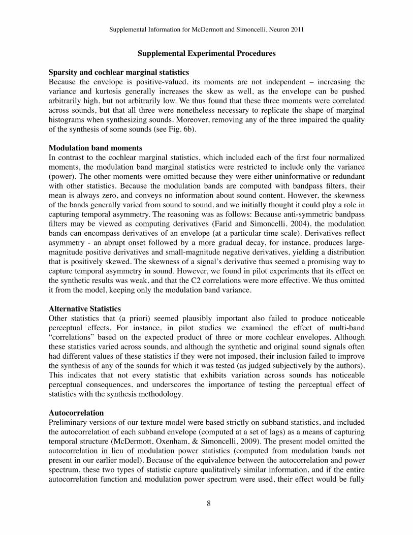
8

Supplemental Experimental Procedures

Sparsity and cochlear marginal statisticsBecause the envelope is positive-valued, its moments are not independent – increasing the variance and kurtosis generally increases the skew as well, as the envelope can be pushed arbitrarily high, but not arbitrarily low. We thus found that these three moments were correlated across sounds, but that all three were nonetheless necessary to replicate the shape of marginal histograms when synthesizing sounds. Moreover, removing any of the three impaired the quality of the synthesis of some sounds (see Fig. 6b).

Modulation band momentsIn contrast to the cochlear marginal statistics, which included each of the first four normalized moments, the modulation band marginal statistics were restricted to include only the variance (power). The other moments were omitted because they were either uninformative or redundant with other statistics. Because the modulation bands are computed with bandpass filters, their mean is always zero, and conveys no information about sound content. However, the skewness of the bands generally varied from sound to sound, and we initially thought it could play a role in capturing temporal asymmetry. The reasoning was as follows: Because anti-symmetric bandpass filters may be viewed as computing derivatives (Farid and Simoncelli, 2004), the modulation bands can encompass derivatives of an envelope (at a particular time scale). Derivatives reflect asymmetry - an abrupt onset followed by a more gradual decay, for instance, produces large-magnitude positive derivatives and small-magnitude negative derivatives, yielding a distribution that is positively skewed. The skewness of a signal’s derivative thus seemed a promising way to capture temporal asymmetry in sound. However, we found in pilot experiments that its effect on the synthetic results was weak, and that the C2 correlations were more effective. We thus omitted it from the model, keeping only the modulation band variance.

Alternative StatisticsOther statistics that (a priori) seemed plausibly important also failed to produce noticeable perceptual effects. For instance, in pilot studies we examined the effect of multi-band “correlations” based on the expected product of three or more cochlear envelopes. Although these statistics varied across sounds, and although the synthetic and original sound signals often had different values of these statistics if they were not imposed, their inclusion failed to improve the synthesis of any of the sounds for which it was tested (as judged subjectively by the authors). This indicates that not every statistic that exhibits variation across sounds has noticeable perceptual consequences, and underscores the importance of testing the perceptual effect of statistics with the synthesis methodology.

AutocorrelationPreliminary versions of our texture model were based strictly on subband statistics, and included the autocorrelation of each subband envelope (computed at a set of lags) as a means of capturing temporal structure (McDermott, Oxenham, & Simoncelli, 2009). The present model omitted the autocorrelation in lieu of modulation power statistics (computed from modulation bands not present in our earlier model). Because of the equivalence between the autocorrelation and power spectrum, these two types of statistic capture qualitatively similar information, and if the entire autocorrelation function and modulation power spectrum were used, their effect would be fully


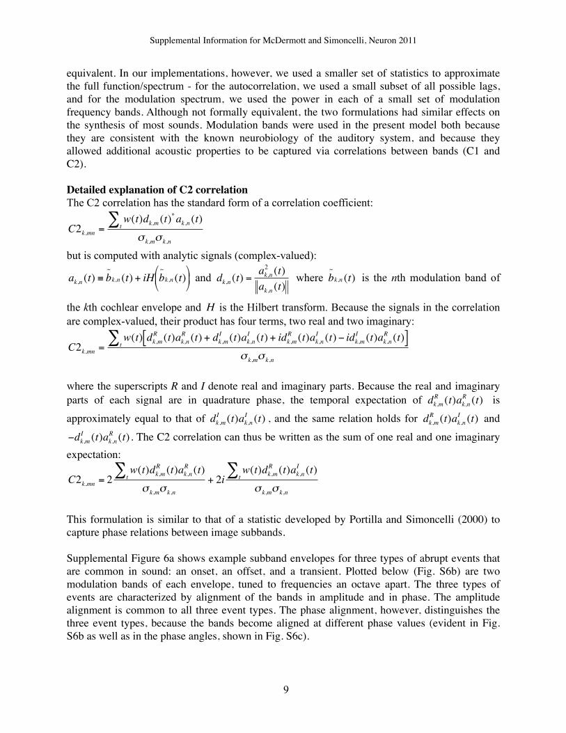
9

equivalent. In our implementations, however, we used a smaller set of statistics to approximate the full function/spectrum - for the autocorrelation, we used a small subset of all possible lags, and for the modulation spectrum, we used the power in each of a small set of modulation frequency bands. Although not formally equivalent, the two formulations had similar effects on the synthesis of most sounds. Modulation bands were used in the present model both because they are consistent with the known neurobiology of the auditory system, and because they allowed additional acoustic properties to be captured via correlations between bands (C1 and C2).

Detailed explanation of C2 correlationThe C2 correlation has the standard form of a correlation coefficient:

€

C2k,mn =w(t)dk,m (t)

*ak,n (t)t∑

σ k,mσ k,n

but is computed with analytic signals (complex-valued):

€

ak,n (t) ≡ b~k,n (t) + iH b

~k,n (t)

and

€

dk,n (t) =ak,n2 (t)ak,n (t)

where

€

b~k,n (t) is the nth modulation band of

the kth cochlear envelope and

€

H is the Hilbert transform. Because the signals in the correlation are complex-valued, their product has four terms, two real and two imaginary:

€

C2k,mn =w(t) dk,m

R (t)ak,nR (t) + dk,m

I (t)ak,nI (t) + idk,m

R (t)ak,nI (t) − idk,m

I (t)ak,nR (t)[ ]t

∑σ k,mσ k,n

where the superscripts R and I denote real and imaginary parts. Because the real and imaginary parts of each signal are in quadrature phase, the temporal expectation of

€

dk,mR (t)ak,n

R (t) is approximately equal to that of

€

dk,mI (t)ak,n

I (t) , and the same relation holds for

€

dk,mR (t)ak,n

I (t) and

€

−dk,mI (t)ak,n

R (t) . The C2 correlation can thus be written as the sum of one real and one imaginary expectation:

€

C2k,mn = 2w(t)dk,m

R (t)ak,nR (t)

t∑

σ k,mσ k,n

+ 2iw(t)dk,m

R (t)ak,nI (t)

t∑

σ k,mσ k,n

This formulation is similar to that of a statistic developed by Portilla and Simoncelli (2000) to capture phase relations between image subbands.

Supplemental Figure 6a shows example subband envelopes for three types of abrupt events that are common in sound: an onset, an offset, and a transient. Plotted below (Fig. S6b) are two modulation bands of each envelope, tuned to frequencies an octave apart. The three types of events are characterized by alignment of the bands in amplitude and in phase. The amplitude alignment is common to all three event types. The phase alignment, however, distinguishes the three event types, because the bands become aligned at different phase values (evident in Fig. S6b as well as in the phase angles, shown in Fig. S6c).


10

It would seem natural to capture this phase alignment by computing a correlation between bands. However, because the bands oscillate at different rates, the phase alignment is momentary – the two bands align and then move away from the point of alignment at different rates (evident in the different slopes of the phase plots in Fig. S6c).

The phase alignment can be transformed into a constant phase difference by doubling the frequency of the lower frequency band. This is accomplished by squaring the analytic version of the band (doubling its frequency and squaring its magnitude), and then dividing by the magnitude to preserve the frequency doubling but retain the original magnitude:

€

dk,n (t) =ak,n2 (t)ak,n (t)

Fig. S6d plots the original band, the magnitude of its analytic signal, and the real part of the frequency-doubled analytic signal. It is apparent that the magnitude is preserved but that the new signal oscillates at twice the rate.

Doubling the frequency of the low band alters its phase at the point of alignment, but because the two bands are an octave apart, the phase of the frequency-doubled low band now advances at the same rate as the high band. This produces a constant phase offset in the vicinity of the original event.

Fig. S6e illustrates this relationship, plotting the phase of the original high frequency band along with that of the frequency-doubled low frequency band. Note that there is now an extended region in which the phase offset between the two signals is relatively constant, and that the offset is different for each of the three event types – a positive step, a negative step, and a brief pulse, respectively. The constant phase offset occurs in the region where the amplitude is high (plotted in Fig. S6f for each band). The phase offset can be made explicit through the product of the two complex signals:

€

dk,m (t)*ak,n (t) , which multiplies the amplitudes and subtracts the phases. When

this complex product is plotted in polar coordinates (Fig. S6g), it is apparent that the high amplitudes occur at particular phase values that are different for each of the three event types. The time-average of this complex product thus yields different values in the three cases. When normalized by the band variances, this time-averaged complex product is the C2 correlation:

€

C2k,mn =w(t)dk,m (t)

*ak,n (t)t∑

σ k,mσ k,n

, the real and imaginary components of which are shown on the

plots in parentheses.

For comparison, Fig. S6h plots the same complex product but without the frequency doubling:

€

ak,m (t)*ak,n (t) . Note that the patterns are now similar in the three cases. A correlation of the

bands without doubling:

€

w(t)ak,m (t)*ak,n (t)t

∑σ k,mσ k,n

thus yields the same values in each case (again

shown on the plots). A standard correlation thus indicates phase alignment, but not the phase


11

value at the point of alignment that is needed to distinguish event types. Our C2 correlation, in contrast, reveals the structure of interest.

Figure S6. The stages involved in computing the C2 correlation (on next page). The stages are illustrated for cochlear channel 8 and modulation bands 2 and 3. (a) Schematic subband envelopes for three event types: an onset, an offset, and a transient. (b) Modulation bands 2 and 3 (tuned to frequencies an octave apart). (c) The phase angles of each band. The location of the event is indicated by the thin black vertical line. (d) The frequency-doubled low band, plotted on top of the original (undoubled) band, and their magnitude. (e) The phase angles of the frequency-doubled low frequency band, and the original high frequency band. The black bracket below the graph indicates the region in which there is a constant phase offset between the bands. (f) Magnitude of each band. (g) Polar plot of the complex product of the frequency-doubled low band and the original high band. The C2 correlation (the vector average of this product, normalized by the standard deviations of the two bands) is shown in parentheses on each plot. (h) The same product computed without frequency doubling, with the corresponding correlation shown in parentheses on each plot.


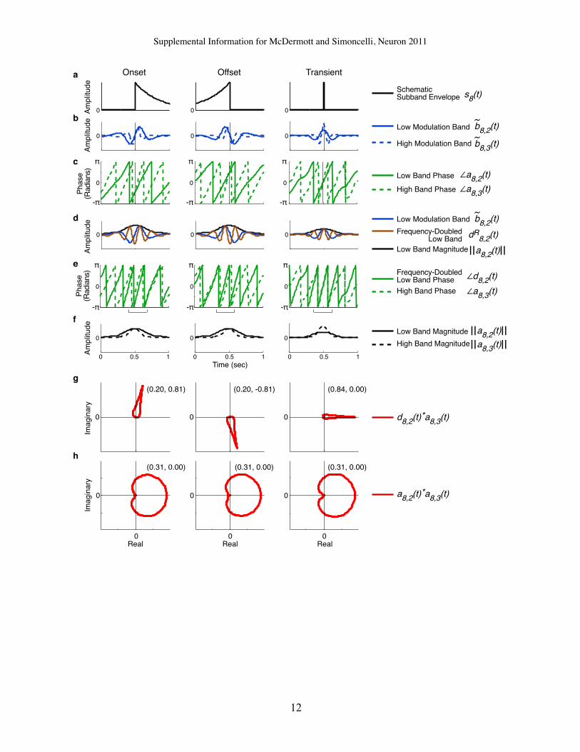
12

(0.31, 0.00)

0

0

0

0

0

0

a

0 0 0

!

-!

0

!

-!

0

!

-!

0

0 0 0

0 0 0

!

-!

0

!

-!

0

!

-!

0

0 0 0

0 0.5 1 0 0.5 1 0 0.5 1

Time (sec)

Real

Onset Offset TransientP

hase"

(Radia

ns)

Phase"

(Radia

ns)

Am

plit

ude

Am

plit

ude

Am

plit

ude

Am

plit

ude

b

c

d

e

f

g

h

Frequency-Doubled"Low Band Phase

High Band Phase

High Band Phase

Low Band Phase

Low Modulation Band

High Modulation Band

Low Modulation Band

Frequency-Doubled""""""""""""""""Low Band

Low Band Magnitude

Schematic"Subband Envelope

High Band Magnitude

Low Band Magnitude

d8,2(t)*a

8,3(t)

a8,2(t)*a

8,3(t)

Real Real

Ima

gin

ary

Ima

gin

ary

∠a8,2(t)

∠a8,3(t)

b8,2(t)

~

b8,3(t)

~

b8,2(t)

~

dR8,2(t)

||a8,2(t)||

∠d8,2(t)

∠a8,3(t)

||a8,2(t)||||a8,3(t)||

s8(t)

0

(0.20, 0.81)

0

(0.20, -0.81)

0

(0.84, 0.00)

(0.31, 0.00) (0.31, 0.00)


13

SoundsOur set of natural sound textures was a mix of in-house recordings made by the authors, files downloaded from online sound repositories, and excerpts from sound effects CDs. The main criterion for inclusion in the set was that the sounds be approximately stationary (as judged subjectively by the authors), because the algorithm was not expected to successfully synthesize non-stationary sounds. See Supp. Table 1 for the full list of sounds. We used 7 sec segments to measure statistics. All sounds were resampled with a sampling rate of 20 kHz and normalized to a fixed rms amplitude.

Psychophysical ExperimentsSubjects performed experiments seated in a sound-attenuating booth (Gretchken Industries). Sounds were presented diotically at 70 dB SPL over Sennheiser HD580 headphones, via a LynxStudio Lynx22 24-bit D/A converter with a sampling rate of 48 kHz. Sounds were synthesized to be 5 sec in duration. The middle 4 sec was excerpted for use in experiments, with 10 ms half-Hanning windows applied to each end. The only exception to this was condition 7 of Experiment 1b, in which 15 sec sounds were synthesized, from which the middle 4 seconds was excerpted for use in the experiment. Multiple synthetic versions were generated for all experimental conditions, (two per condition for Experiments 1-3, and three for Experiment 4), one of which was randomly chosen on each trial of an experiment (except for Experiment 4, in which listeners were presented with all three versions on separate trials). All participants were non-expert listeners and were naïve as to the purpose of the experiments.

Experiment 1a: IdentificationOn each trial, participants heard a 4 sec excerpt of either an original sound recording, or a synthetic signal with some subset of our model’s statistics matched to those of an original recording. They then selected a name for the sound from a list of five, by clicking a mouse. The sounds were drawn from a subset of 96 of the 168 sounds in our set, the sound of which we thought likely to be familiar to undergraduate subjects. These sounds were organized into groups whose sounds we thought were likely to be confusable (e.g. rain and river, WWII bomber plane and construction noise), and the incorrect choices on a trial were constrained not to be drawn from the sound’s confusion group. All sounds were used once per condition, for a total of 864 trials completed in pseudo-random order. Ten subjects participated (9 female), averaging 22.2 years of age. Subjects in Experiments 1a and 1b were not given practice trials, and had not participated in any of our other experiments, such that they had never heard any of the sounds or their synthetic versions prior to starting the experiment.

Experiment 1b: Identification, Part 2The procedure for Experiment 1b was identical to that of Experiment 1a. Ten subjects participated (8 female) averaged 20.2 years of age.

Experiments 1b and 1c utilized alternative models to test various hypotheses of interest. Two conditions featured sounds synthesized using a model with broader or narrower filters than those in our canonical model (whose filters were approximately matched to those of the human


14

auditory system). In these cases we used 7 and 120 filters, respectively, covering the same frequency range, again equally spaced on an ERB scale, with adjacent filters overlapping by 50%, and with lowpass and highpass filters on each end of the spectrum to assure perfect tiling (and thus invertibility). Another condition used a model with the same filter bandwidths as the canonical model, but with neighboring filters that overlapped by 87.5%, producing four times as many filters over the same spectral range. These filter banks also had lowpass and highpass filters on the ends to produce perfect tiling. We also included a condition in both experiments in which our canonical texture model was supplemented with marginal histogram matching, using 128 bins per histogram (Heeger and Bergen, 1995).

Experiment 1c: Realism of Synthesis with Alternative Marginal StatisticsExperiment 1c extended the identification results of Experiment 1b by comparing the realism of sounds synthesized with different kinds of marginal statistics – those measured from our canonical model, or from alternative models, either with different filters or with a more comprehensive description of the filter marginal distributions. The results are shown in Figs. S3 and S4.

The procedure was identical to that of Experiments 2 and 3 (described in full below). On each trial, participants heard an excerpt of an original recording followed by two synthetic excerpts, and selected the synthetic example that sounded like a more realistic example of the original. All synthetic excerpts were synthesized by imposing the “cochlear” marginal statistics of the original recording. One of the synthetic examples was always generated using biologically faithful cochlear bandwidths and the four marginal moments of our canonical model. The other synthetic example was generated using filters four times narrower (condition 1), filters four times broader (condition 2), four times as many filters with the same bandwidth (condition 3), or the filters of the canonical model, but using the full marginal histogram in addition to the marginal moments (condition 4).

Experiment 1c used a smaller subset of 48 sound recordings that were subjectively judged to lack strong temporal structure (because the marginal statistics did not greatly constrain temporal structure, and we wanted to avoid large numbers of trials where both synthetic examples bore little resemblance to the original sound). All sounds were used in all conditions, yielding 192 trials, completed in random order. For the analysis of Fig. S3, sounds were grouped into 12 classes, each containing at least two sounds. Ten subjects participated (8 female), averaging 23.7 years of age.

Experiment 2a: OmissionOn each trial, participants heard a 4 sec excerpt of an original sound recording followed by two synthetic versions, with 400 ms of silence between sounds. One synthetic version was synthesized with the full set of statistics, and the other with all but one class of statistics. In the marginal condition, the envelope variance, skew, and kurtosis were omitted (the mean was left in to ensure the correct spectrum). The order in which the two versions were presented was randomized. Listeners selected which version sounded like a more realistic example of the original. Ninety-eight original sounds (and their synthetic versions) were used. Each sound was


15

presented once per condition, for a total of 490 trials, completed in random order. All subjects were given 20 practice trials prior to starting the experiment. Ten subjects participated (8 female), averaging 24.4 years of age.

The sound set was slightly different from that used in Experiment 1 – some of the multiple versions of certain sound classes were removed to reduce redundancy, replaced by sounds that were omitted from Experiment 1 for reasons of their unfamiliarity (e.g. a “teletype”, which most undergraduates are unfamiliar with, but for which original and synthetic versions are readily compared). The asymmetric sounds included in the analysis of C2 correlation omission were: Typewriter – manual, Typewriter – IBM electric, Drumroll, Battle explosions, Tapping on hard surface, Hammering copper, Snare drum beats, Bongo loop, Reverse drum beats – snare, Teletype, Firecrackers, and Rhythmic applause. 30000 other randomly chosen subsets of sounds were evaluated for comparison.

Experiment 2b :Marginal VariantsThe trial format and set of sounds was identical to that of Experiment 2a. In every condition, one of the two synthetic versions was synthesized with the full set of statistics measured in the original sound. In condition 1, the other synthetic sound was given the envelope variance, skew and kurtosis of pink noise (measured from a 30 sec excerpt), with the other statistics taken from the original recording, including the envelope mean, which ensured that the spectrum was faithful to the original. The synthesis process succeeded in synthesizing signals with the desired statistics despite the artificial combination (as verified with the same SNR measurements used in other experimental stimuli). In condition 2, the marginal moments were omitted from synthesis but the other statistics were set to the values of the original sound (this conditions was equivalent to condition 1 of Experiment 2a, but was repeated because the subjects in the two experiments were different). In condition 3, only the skew and kurtosis were omitted from synthesis. Nine female subjects participated, averaging 24.1 years of age.

Experiment 3: Nonbiological ModelsThe format of this experiment was identical to that of Experiment 2a&b, and the same sounds were used. The participant group had not participated in the other experiments, to avoid the possibility that participants might have learned the sound of our original model in previous experiments. Eight subjects participated (5 female), averaging 25 years of age.

Linearly-spaced filters were substituted for the acoustic (cochlear) and modulation filterbanks in some of the conditions. The linear acoustic filterbank had the same number of filters as that in the original model, and was identically generated except that the frequency responses were half-cosines on a linear scale rather than an ERB scale, with a fixed bandwidth of 321.9 Hz. The linearly-spaced filters thus tiled the spectrum as did the ERB filter bank, and produced the same number of statistical measurements, but divided up the spectrum differently.

The linear modulation filterbank also had 20 filters, with peak frequencies ranging from .5 to 200 Hz in 10.5 Hz intervals. The frequency responses were half-cosines with a fixed bandwidth of


16

17.04 Hz, which produced the same degree of overlap between the passbands (defined by the 3dB-down points) of adjacent filters (38.4%) as was present in the constant Q filterbank (averaging the overlap on the low and high end of a filter). The two lowest filters had a slightly different frequency response to avoid including DC – they increased with a cosine ramp from 0 Hz to their peak frequency. The highest filter cut off at the peak of its frequency response; i.e. it was a quarter-cosine (this was to ensure that all modulation frequencies were represented in the bank).

Because the C2 correlations could only be computed with octave-spaced filters, it was not possible to alter the filter bank used to measure and impose them, and we omitted them from the conditions using a linear modulation filterbank (as well as in the comparison stimuli generated with the biologically plausible model). However, the C1 correlations presented no such limitation, and for them we used a linear filter bank that tiled the spectrum and had comparable overlap to the octave-spaced modulation filter bank in our standard model. The peak frequencies ranged from 3.1 to 167.2 Hz in steps of 32.8 Hz (half-cosine frequency responses with bandwidths of 32.8 Hz, except for the lowest frequency filter, which ramped from 0 to its peak frequency, again to avoid including DC).

Note that the superior realism we observed for the biological texture model could not be explained simply by a difference in how well the biological and nonbiological statistics were imposed. SNRs were comparable between conditions. Synthesis with the nonbiological model averaged 36.26, 45.31, 33.64, and 45.06 dB (conditions 1-4), compared to 35.75 (condition 1) and 38.01 dB (conditions 2-4; no C2 correlations) for the original syntheses used as a comparison.

The choice of which cochlear correlations (i.e., which offsets) to include in the model was informally optimized in pilot tests using the biological model. It might be argued that different choices would be optimal for the nonbiological model with linearly spaced filters, and that the chosen offsets, even if themselves imposed faithfully, would thus be less likely to instantiate the full correlation structure between channels. To address this possibility, we checked the fidelity with which the full correlation matrix was imposed for both models (in dB SNR). There was no significant difference (paired t-test, p=.06), and if anything, the SNR for the full correlation matrix was slightly higher for the nonbiological model with the linearly spaced filter bank than for our canonical biologically plausible model (18.04 dB vs. 18.60 dB, SE=.70 and .75). We performed the same sort of analysis for the C1 correlations, and obtained a similar result: slightly higher SNRs for the nonbiological model (8.75 dB vs. 10.36 dB, SE=.55 and .63; the lower SNRs here are due to the fact that only two offsets were imposed for this statistic). Although we cannot exclude the possibility that some alternative non-biological model would produce better synthetic results, the differences in synthesis quality we observed do not appear to be due to the choices that were made about the number of statistics to include.


17

Experiment 4: Realism RatingsOn each trial, participants heard a 4 sec excerpt of an original sound recording followed by a synthetic version of the original, with 400 ms of silence between sounds. The synthetic version was synthesized with the full set of statistics. Participants were instructed to judge the extent to which the synthetic version sounded like another example of the original sound. They selected a rating on a scale of 1-7 by clicking a mouse, with 7 indicating the highest degree of realism and 1 the lowest. The full set of 168 original sounds (and their synthetic versions) was used. The experiment cycled through the set of sounds three times, each time in a different random order and with a different synthetic exemplar. Ten subjects participated (7 female), averaging 20 years of age.

Supplemental References

Farid, H., and Simoncelli, E.P. (2004). Differentiation of multi-dimensional signals. IEEE Transactions on Image Processing 13, 496-508.Heeger, D.J., and Bergen, J. (1995). Pyramid-based texture analysis/synthesis. Computer Graphics (ACM SIGGRAPH Proceedings), 229-238.McDermott, J.H., Oxenham, A.J., and Simoncelli, E.P. (2009). Sound texture synthesis via filter statistics. In IEEE Workshop on Applications of Signal Processing to Audio and Acoustics (New Paltz, New York), pp. 297-300.Portilla, J., and Simoncelli, E.P. (2000). A parametric texture model based on joint statistics of complex wavelet coefficients. International Journal of Computer Vision 40, 49-71.


Sound Texture Perception via Statistics of the Auditory...

Documents

Transcript of Sound Texture Perception via Statistics of the Auditory...