
Sort Algorithms - Vancouver Island University
50
Sort Algorithms Humayun Kabir Professor, CS, Vancouver Island University, BC, Canada
Transcript of Sort Algorithms - Vancouver Island University

Sort Algorithms
Humayun KabirProfessor, CS, Vancouver Island University, BC, Canada

Sorting
• Sorting is a process that organizes a collection of data
into either ascending or descending order.
• An internal sort requires that the collection of data fit
entirely in the computer’s main memory.
• We can use an external sort when the collection of
data cannot fit in the computer’s main memory all at
once but must reside in secondary storage such as on a
disk.
• We will analyze only internal sorting algorithms.

Sorting
• Any significant amount of computer output is generally
arranged in some sorted order so that it can be
interpreted.
• Sorting also has indirect uses. An initial sort of the data
can significantly enhance the performance of an
algorithm.
• Majority of programming projects use a sort
somewhere, and in many cases, the sorting cost
determines the running time.
• A comparison-based sorting algorithm makes ordering
decisions only on the basis of comparisons.
Sorting Algorithms
• There are many comparison based sorting algorithms, such as:
– Bubble Sort
– Selection Sort
– Insertion Sort
– Merge Sort
– Quick Sort

Bubble Sort
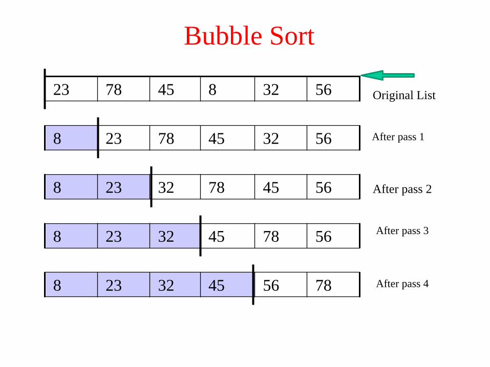
• The list is divided into two sublists: sorted and unsorted.
• Starting from the bottom of the list, the smallest element isbubbled up from the unsorted list and moved to the sortedsublist.
• After that, the wall moves one element ahead, increasingthe number of sorted elements and decreasing the numberof unsorted ones.
• Each time an element moves from the unsorted part to thesorted part one sort pass is completed.
• Given a list of n elements, bubble sort requires up to n-1passes to sort the data.
Bubble Sort
23 78 45 8 32 56
8 23 78 45 32 56
8 23 32 78 45 56
8 23 32 45 78 56
8 23 32 45 56 78
Original List
After pass 1
After pass 2
After pass 3
After pass 4

Bubble Sort Algorithm
void bubleSort(int a[], int n) {
bool sorted = false;
int last = n-1;
for (int i = 0; (i < last) && !sorted; i++){
sorted = true;
for (int j=last; j > i; j--)
if (a[j-1] > a[j]{
swap(a[j],a[j-1]);
sorted = false; // signal exchange
}
}
}
void swap( int &lhs, int &rhs ){int tmp = lhs;lhs = rhs;rhs = tmp;
}

Bubble Sort – Analysis
• In general, we compare keys and move items (or
exchange items) in a sorting algorithm (which
uses key comparisons).
So, to analyze a sorting algorithm we
should count the number of key comparisons
and the number of moves.
• Ignoring other operations does not affect our final
result.

Bubble Sort – Analysis
• Best-case: O(n)– Array is already sorted in ascending order.
– The number of moves: 0 O(1)
– The number of key comparisons: (n-1) O(n)
• Worst-case: O(n2)– Array is in reverse order:
– Outer loop is executed n-1 times,
– The number of moves: 3*(1+2+...+n-1) = 3 * n*(n-1)/2 O(n2)
– The number of key comparisons: (1+2+...+n-1)= n*(n-1)/2 O(n2)
• Average-case: O(n2)– We have to look at all possible initial data organizations.
• So, Bubble Sort is O(n2)
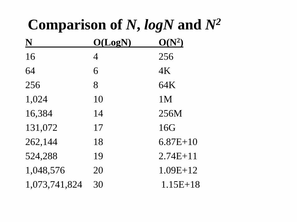
Comparison of N, logN and N2
N O(LogN) O(N2)
16 4 256
64 6 4K
256 8 64K
1,024 10 1M
16,384 14 256M
131,072 17 16G
262,144 18 6.87E+10
524,288 19 2.74E+11
1,048,576 20 1.09E+12
1,073,741,824 30 1.15E+18

Selection Sort
• The list is divided into two sublists, sorted and unsorted,which are divided by an imaginary wall.
• We find the smallest element from the unsorted sublist andswap it with the element at the beginning of the unsorteddata.
• After each selection and swapping, the imaginary wallbetween the two sublists move one element ahead,increasing the number of sorted elements and decreasingthe number of unsorted ones.
• Each time we move one element from the unsorted sublistto the sorted sublist, we say that we have completed a sortpass.
• A list of n elements requires n-1 passes to completelyrearrange the data.

23 78 45 8 32 56
8 78 45 23 32 56
8 23 45 78 32 56
8 23 32 78 45 56
8 23 32 45 78 56
8 23 32 45 56 78
Original List
After pass 1
After pass 2
After pass 3
After pass 4
After pass 5
Sorted Unsorted
Selection Sort

Selection Sort
void selectionSort( int a[], int n) {
for (int i = 0; i < n-1; i++) {
int min = i;
for (int j = i+1; j < n; j++)
if (a[j] < a[min]) min = j;
swap(a[i], a[min]);
}
}

Selection Sort -- Analysis
• In selectionSort function, the outer for loop executes n-1 times.
• We invoke swap function once at each iteration.
Total Swaps: n-1
Total Moves: 3*(n-1) (Each swap has three moves)

Selection Sort – Analysis (cont.)
• The inner for loop executes the size of the unsorted part minus 1
(from 1 to n-1), and in each iteration we make one key
comparison.
# of key comparisons = 1+2+...+n-1 = n*(n-1)/2
So, Selection sort is O(n2)
• The best case, the worst case, and the average case of the
selection sort algorithm are same. all of them are O(n2)
– This means that the behavior of the selection sort algorithm does not depend on the
initial organization of data.
– Since O(n2) grows so rapidly, the selection sort algorithm is appropriate only for
small n.
– Although the selection sort algorithm requires O(n2) key comparisons, it only
requires O(n) moves.
– A selection sort could be a good choice if data moves are costly but key
comparisons are not costly (short keys, long records).

Insertion Sort
• Insertion sort is a simple sorting algorithm that is appropriate for small inputs.
– Most common sorting technique used by card players.
• The list is divided into two parts: sorted and unsorted.
• In each pass, the first element of the unsorted part is picked up, transferred to the sorted sublist, and inserted at the appropriate place.
• A list of n elements will take at most n-1 passes to sort the data.

Original List
After pass 1
After pass 2
After pass 3
After pass 4
After pass 5
23 78 45 8 32 56
23 78 45 8 32 56
23 45 78 8 32 56
8 23 45 78 32 56
8 23 32 45 78 56
8 23 32 45 56 78
Sorted Unsorted
Insertion Sort

Insertion Sort Algorithm
void insertionSort(int a[], int n) {
for (int i = 1; i < n; i++)
{
int tmp = a[i];
for (int j=i; j>0 && tmp < a[j-1]; j--)
a[j] = a[j-1];
a[j] = tmp;
}
}

Insertion Sort – Analysis
• Running time depends on not only the size of the array but also the contents of the array.
• Best-case: O(n)– Array is already sorted in ascending order.
– Inner loop will not be executed.
– The number of moves: 2*(n-1) O(n)
– The number of key comparisons: (n-1) O(n)
• Worst-case: O(n2)– Array is in reverse order:
– Inner loop is executed i-1 times, for i = 2,3, …, n
– The number of moves: 2*(n-1)+(1+2+...+n-1)= 2*(n-1)+ n*(n-1)/2 O(n2)
– The number of key comparisons: (1+2+...+n-1)= n*(n-1)/2 O(n2)
• Average-case: O(n2)– We have to look at all possible initial data organizations.
• So, Insertion Sort is O(n2)
Analysis of Insertion sort
• Which running time will be used to characterize this
algorithm?
– Best, worst or average?
• Worst:
– Longest running time (this is the upper limit for the algorithm)
– It is guaranteed that the algorithm will not be worse than this.
• Sometimes we are interested in average case. But there are
some problems with the average case.
– It is difficult to figure out the average case. i.e. what is average
input?
– Are we going to assume all possible inputs are equally likely?
– In fact for most algorithms average case is same as the worst case.

Mergesort
• Mergesort algorithm is one of two important divide-and-conquer
sorting algorithms (the other one is quicksort).
• It is a recursive algorithm.
– Divides the list into halves,
– Sort each halve separately, and
– Then merge the sorted halves into one sorted array.
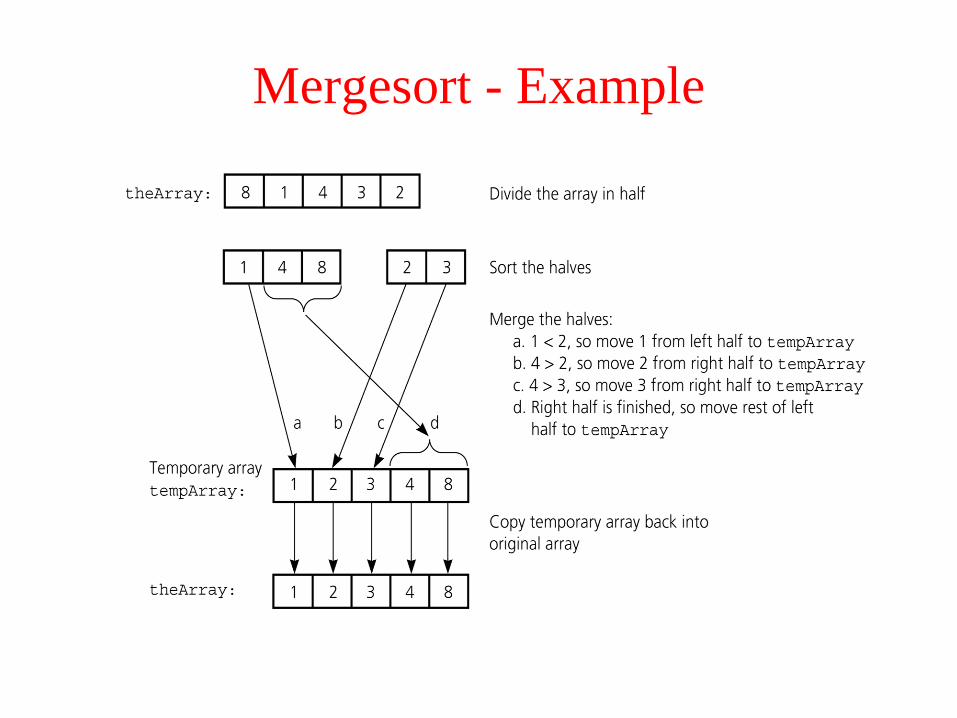
Mergesort - Example
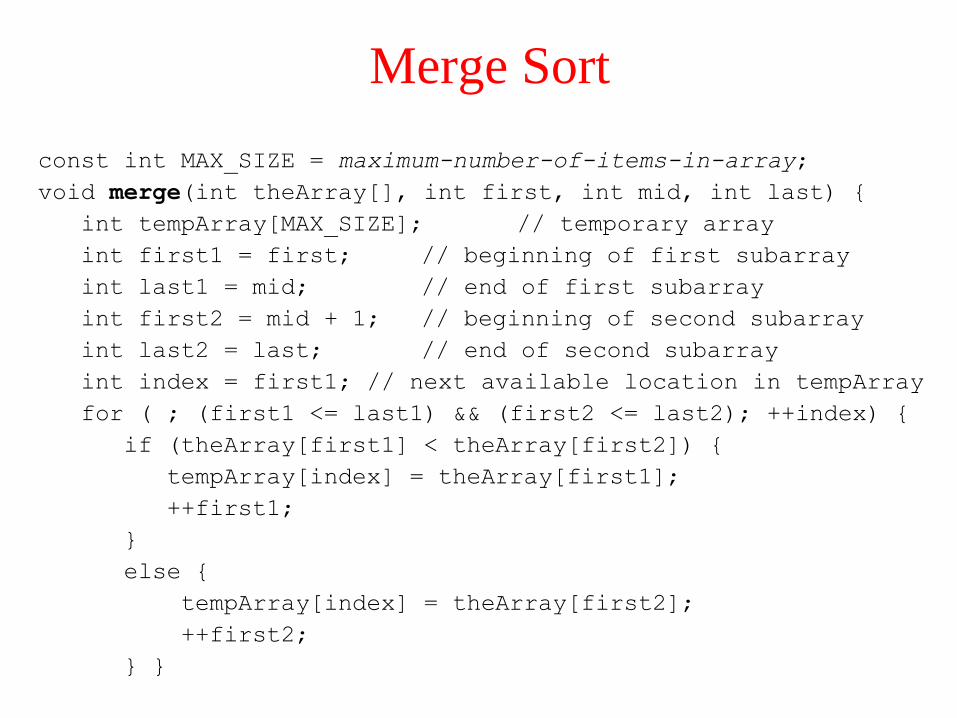
Merge Sort
const int MAX_SIZE = maximum-number-of-items-in-array;
void merge(int theArray[], int first, int mid, int last) {
int tempArray[MAX_SIZE]; // temporary array
int first1 = first; // beginning of first subarray
int last1 = mid; // end of first subarray
int first2 = mid + 1; // beginning of second subarray
int last2 = last; // end of second subarray
int index = first1; // next available location in tempArray
for ( ; (first1 <= last1) && (first2 <= last2); ++index) {
if (theArray[first1] < theArray[first2]) {
tempArray[index] = theArray[first1];
++first1;
}
else {
tempArray[index] = theArray[first2];
++first2;
} }

Merge Sort (cont.)
// finish off the first subarray, if necessary
for (; first1 <= last1; ++first1, ++index)
tempArray[index] = theArray[first1];
// finish off the second subarray, if necessary
for (; first2 <= last2; ++first2, ++index)
tempArray[index] = theArray[first2];
// copy the result back into the original array
for (index = first; index <= last; ++index)
theArray[index] = tempArray[index];
} // end merge

Merge Sort
void mergesort(int theArray[], int first, int last) {
if (first < last) {
int mid = (first + last)/2; // index of midpoint
mergesort(theArray, first, mid);
mergesort(theArray, mid+1, last);
// merge the two halves
merge(theArray, first, mid, last);
}
} // end mergesort

Merge Sort - Example
6 3 9 1 5 4 7 2
5 4 7 26 3 9 1
6 3 9 1 7 2
5 4
6 3 19 5 4 27
3 6 1 9 2 7
4 5
2 4 5 71 3 6 9
1 2 3 4 5 7 8 9
divide
dividedividedivide
dividedivide
divide
merge merge
merge
merge
merge merge
merge

Mergesort – Example2

Mergesort – Analysis of Merge
A worst-case instance of the merge step in mergesort

Mergesort – Analysis of Merge (cont.)
Merging two sorted arrays of size k
• Best-case:
– All the elements in the first array are smaller (or larger) than all the
elements in the second array.
– The number of moves: 2k + 2k
– The number of key comparisons: k
• Worst-case:
– The number of moves: 2k + 2k
– The number of key comparisons: 2k-1
...... ......
......
0 k-1 0 k-1
0 2k-1

Mergesort - Analysis
Levels of recursive calls to mergesort, given an array of eight items
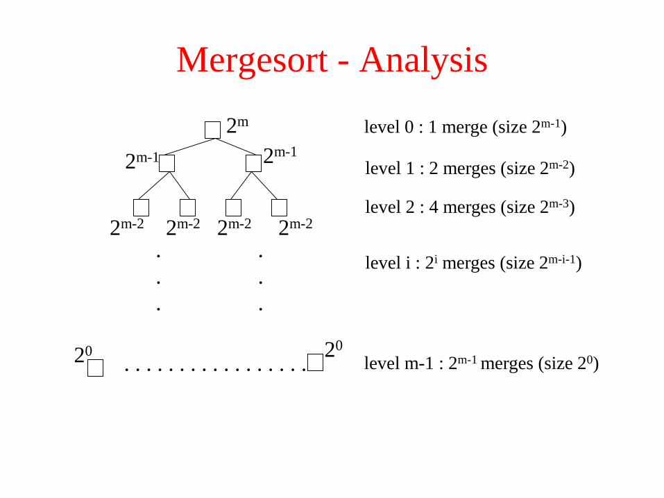
Mergesort - Analysis
.
.
.
.
.
.
. . . . . . . . . . . . . . . . .
2m
2m-1 2m-1
2m-2 2m-2 2m-2 2m-2
20 20
level 0 : 1 merge (size 2m-1)
level 1 : 2 merges (size 2m-2)
level 2 : 4 merges (size 2m-3)
level m-1 : 2m-1 merges (size 20)
level i : 2i merges (size 2m-i-1)
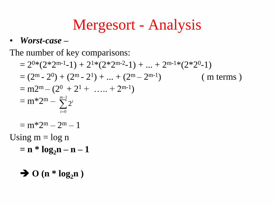
Mergesort - Analysis• Worst-case –
The number of key comparisons:
= 20*(2*2m-1-1) + 21*(2*2m-2-1) + ... + 2m-1*(2*20-1)
= (2m - 20) + (2m - 21) + ... + (2m – 2m-1) ( m terms )
= m2m – (20 + 21 + ….. + 2m-1)
= m*2m –
= m*2m – 2m – 1
Using m = log n
= n * log2n – n – 1
O (n * log2n )
1
0
2m
i
i

Mergesort – Analysis• Mergesort is extremely efficient algorithm with respect
to time.– Both worst case and average cases are O (n * log2n )
• But, mergesort requires an extra array whose size
equals to the size of the original array.
• If we use a linked list, we do not need an extra array – But, we need space for the links
– And, it will be difficult to divide the list into half ( O(n) )
Quicksort
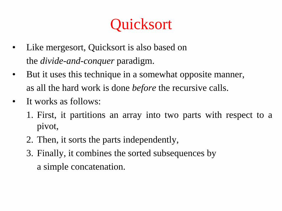
• Like mergesort, Quicksort is also based on
the divide-and-conquer paradigm.
• But it uses this technique in a somewhat opposite manner,
as all the hard work is done before the recursive calls.
• It works as follows:
1. First, it partitions an array into two parts with respect to a
pivot,
2. Then, it sorts the parts independently,
3. Finally, it combines the sorted subsequences by
a simple concatenation.

Quicksort (cont.)
The quick-sort algorithm consists of the following three steps:
1. Divide: Partition the list.
– To partition the list, we first choose some element from the list
for which we hope about half the elements will come before
and half after. Call this element the pivot.
– Then we partition the elements so that all those with values
less than the pivot come in one sublist and all those with
greater values come in another.
2. Recursion: Recursively sort the sublists separately.
3. Conquer: Put the sorted sublists together.

Quick Sort Partition
• Partitioning places the pivot in its correct place position within the array.
• Arranging the array elements around the pivot p generates two smaller sorting
problems.
– sort the left section of the array, and sort the right section of the array.
– when these two smaller sorting problems are solved recursively, our bigger
sorting problem is solved.

Partition – Choosing the pivot
• First, we have to select a pivot element among the elements of the
given array, and we put this pivot into the first location of the
array before partitioning.
• Which array item should be selected as pivot?
– Somehow we have to select a pivot, and we hope that we will
get a good partitioning.
– If the items in the array arranged randomly, we choose a pivot
randomly.
– We can choose the first or last element as a pivot (it may not
give a good partitioning).
– We can use different techniques to select the pivot.

Partition Function
void partition(int theArray[], int first, int last,
int &pivotIndex) {
// Partitions an array for quicksort.
// Precondition: first <= last.
// Postcondition: Partitions theArray[first..last] such that:
// S1 = theArray[first..pivotIndex-1] < pivot
// theArray[pivotIndex] == pivot
// S2 = theArray[pivotIndex+1..last] >= pivot
// Calls: choosePivot and swap.
// place pivot in theArray[first]
choosePivot(theArray, first, last);
int pivot = theArray[first]; // copy pivot
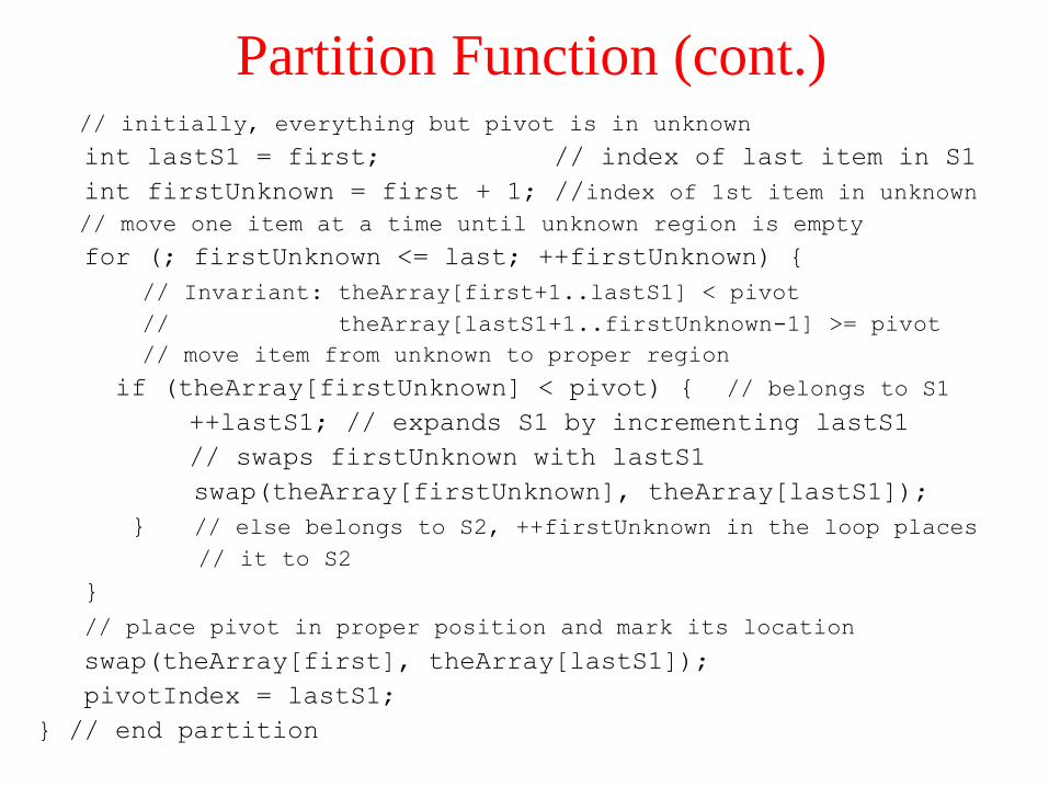
Partition Function (cont.)// initially, everything but pivot is in unknown
int lastS1 = first; // index of last item in S1
int firstUnknown = first + 1; //index of 1st item in unknown
// move one item at a time until unknown region is empty
for (; firstUnknown <= last; ++firstUnknown) {
// Invariant: theArray[first+1..lastS1] < pivot
// theArray[lastS1+1..firstUnknown-1] >= pivot
// move item from unknown to proper region
if (theArray[firstUnknown] < pivot) { // belongs to S1
++lastS1; // expands S1 by incrementing lastS1
// swaps firstUnknown with lastS1
swap(theArray[firstUnknown], theArray[lastS1]);
} // else belongs to S2, ++firstUnknown in the loop places
// it to S2
}
// place pivot in proper position and mark its location
swap(theArray[first], theArray[lastS1]);
pivotIndex = lastS1;
} // end partition

Partition Function (cont.)
Invariant for the partition algorithm
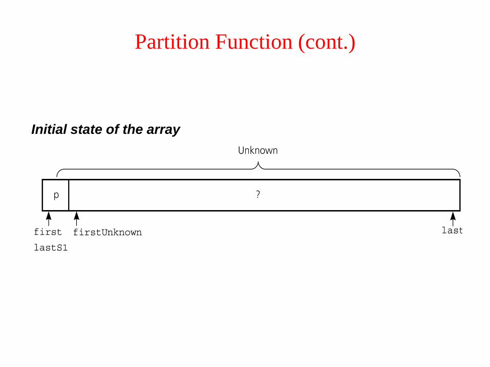
Partition Function (cont.)
Initial state of the array
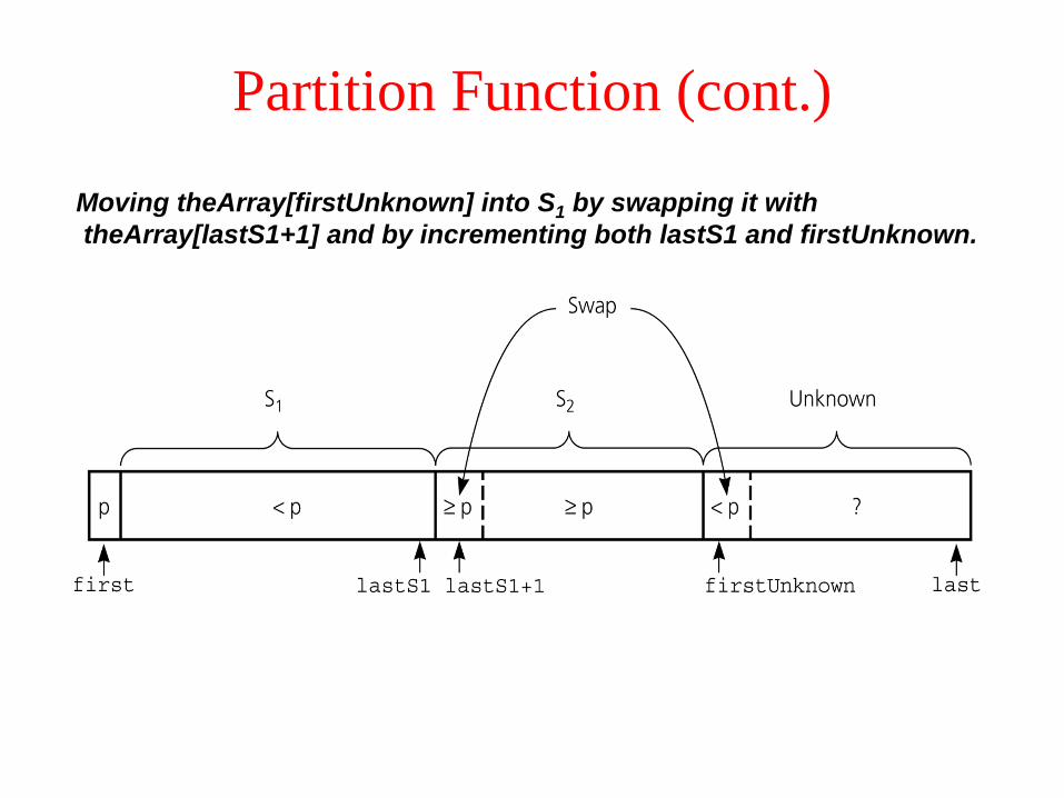
Partition Function (cont.)
Moving theArray[firstUnknown] into S1 by swapping it with
theArray[lastS1+1] and by incrementing both lastS1 and firstUnknown.

Partition Function (cont.)
Moving theArray[firstUnknown] into S2 by incrementing firstUnknown.

Partition Function (cont.)
Developing the first
partition of an array
when the pivot is the
first item

Quicksort Function
void quicksort(int theArray[], int first, int last) {
// Sorts the items in an array into ascending order.
// Precondition: theArray[first..last] is an array.
// Postcondition: theArray[first..last] is sorted.
// Calls: partition.
int pivotIndex;
if (first < last) {
// create the partition: S1, pivot, S2
partition(theArray, first, last, pivotIndex);
// sort regions S1 and S2
quicksort(theArray, first, pivotIndex-1);
quicksort(theArray, pivotIndex+1, last);
}
}

Quicksort – Analysis
An average-
case
partitioning
with quicksort

Quicksort – Analysis
• Quicksort is O(n*log2n) in the best case and average case.
• Quicksort is slow when the array is sorted and we choose the first
element as the pivot.
• Although the worst case behavior is not so good, its average case
behavior is much better than its worst case.
– So, Quicksort is one of best sorting algorithms using key comparisons.

Quicksort – Analysis
A worst-case partitioning with quicksort

Quicksort – Analysis
Worst Case: (assume that we are selecting the first element as pivot)
– The pivot divides the list of size n into two sublists of sizes 0 and n-1.
– The number of key comparisons
= n-1 + n-2 + ... + 1
= n(n-1)/2
= n2/2 – n/2 O(n2)
– The number of swaps =
= ( n-1 + n-2 + ... + 1) + (n-1)
= (n-1) + n(n-1)/2
= n2/2 + n/2 - 1 O(n2)
• So, Quicksort is O(n2) in worst case
swaps outside of
the for loop
swaps inside of
the for loop

Comparison of Sorting Algorithms