SOOT MASS ESTIMATION FROM ELECTRICAL CAPACITANCE ...
61
SOOT MASS ESTIMATION FROM ELECTRICAL CAPACITANCE TOMOGRAPHY IMAGING FOR A DIESEL PARTICULATE FILTER A Thesis Submitted to the Faculty of Purdue University by Salah E. Hassan In Partial Fulfillment of the Requirements for the Degree of Master of Science in Mechanical Engineering May 2020 Purdue University Indianapolis, Indiana
Transcript of SOOT MASS ESTIMATION FROM ELECTRICAL CAPACITANCE ...
SOOT MASS ESTIMATION FROM ELECTRICAL CAPACITANCE
TOMOGRAPHY IMAGING FOR A DIESEL PARTICULATE FILTER
A Thesis
Submitted to the Faculty
of
Purdue University
by
Salah E. Hassan
In Partial Fulfillment of the
Requirements for the Degree
of
Master of Science in Mechanical Engineering
May 2020
Purdue University
Indianapolis, Indiana

ii
THE PURDUE UNIVERSITY GRADUATE SCHOOL
STATEMENT OF THESIS APPROVAL
Dr. Sohel Anwar, Chair
Department of Mechanical and Energy Engineering
Dr. Hazim El-Mounayri
Department of Mechanical and Energy Engineering
Dr. Andres Tovar
Department of Mechanical and Energy Engineering
Approved by:
Dr. Sohel Anwar
Chair of the Graduate Program

iii
This Thesis is dedicated to the memory of my parents, Karar and Shadia, to my
beloved small family, my sister, Samira, my wife, Nosayba, my darling kids,
Mohamed and Shadia.

iv
ACKNOWLEDGMENTS
I would like to express my sincere gratefulness to my advisor Dr. Sohel Anwar, for his
continuous support throughout the course of my thesis and study, for his patience,
motivation, knowledge.His guidance was a valuable key in my success of this project.
Besides my advisor, I would like to thank the rest of my thesis committee. Dr.Hazim,
and Dr. Tovar, for their deep, and insightful comments, and hard questions.
My sincere thanks also goes to my colleagues, Mohamed Khattab (Mechanical En-
gineering), Ammar Ali (Mechanical Engineering) , Adish Krishna(Mechanical Engi-
neering) , Omar Siedahmed (Electrical Engineering).

v
TABLE OF CONTENTS
Page
LIST OF TABLES . . . . . . . . . . . . . . . . . . . . . . . . . . . . . . . . . . vii
LIST OF FIGURES . . . . . . . . . . . . . . . . . . . . . . . . . . . . . . . . . viii
SYMBOLS . . . . . . . . . . . . . . . . . . . . . . . . . . . . . . . . . . . . . . x
ABBREVIATIONS . . . . . . . . . . . . . . . . . . . . . . . . . . . . . . . . . . xi
ABSTRACT . . . . . . . . . . . . . . . . . . . . . . . . . . . . . . . . . . . . . xii
1 INTRODUCTION . . . . . . . . . . . . . . . . . . . . . . . . . . . . . . . . 1
1.1 Overview . . . . . . . . . . . . . . . . . . . . . . . . . . . . . . . . . . . 1
1.2 Problem Statement . . . . . . . . . . . . . . . . . . . . . . . . . . . . . 3
1.3 Research Objective . . . . . . . . . . . . . . . . . . . . . . . . . . . . . 4
2 ELECTRICAL CAPACITANCE TOMOGRAPHY (ECT) - LITERATUREREVIEW . . . . . . . . . . . . . . . . . . . . . . . . . . . . . . . . . . . . . 6
3 DESIGN OF AN ELECTRICAL CAPACITANCE TOMOGRAPHY SYSTEM 9
3.1 ECT Model Design . . . . . . . . . . . . . . . . . . . . . . . . . . . . . 9
3.2 Image Reconstruction . . . . . . . . . . . . . . . . . . . . . . . . . . . . 10
3.2.1 Image Reconstruction using Linear Back Projection . . . . . . 11
3.2.2 Direct Techniques to Generate Sensitivity Matrix . . . . . . . . 12
3.2.3 Soot Load Estimation from Pixel Gray-Level Value . . . . . . . 12
4 SOOT MASS ESTIMATION FROM RECONSTRUCTED IMAGE . . . . 13

vi
Page
4.1 Soot Mass Estimation . . . . . . . . . . . . . . . . . . . . . . . . . . . 17
4.2 Computational Results and Discussion . . . . . . . . . . . . . . . . . . 21
5 VALIDATION OF SOOT ESTIMATION USING FINITE ELEMENT ANAL-YSIS . . . . . . . . . . . . . . . . . . . . . . . . . . . . . . . . . . . . . . . . 23
5.1 ANSYS Electronic Maxwell 3D Model . . . . . . . . . . . . . . . . . . 23
5.2 Geometric Model . . . . . . . . . . . . . . . . . . . . . . . . . . . . . 25
5.3 Material Selection . . . . . . . . . . . . . . . . . . . . . . . . . . . . . . 26
5.4 Electrodes Voltage and Solution Matrix . . . . . . . . . . . . . . . . . . 27
5.5 Voltage Distribution Simulation . . . . . . . . . . . . . . . . . . . . . . 28
5.6 Sensitivity Matrix . . . . . . . . . . . . . . . . . . . . . . . . . . . . . 29
5.7 Capacitance Data Collection . . . . . . . . . . . . . . . . . . . . . . . . 31
5.8 Circumferential Distributed Soot . . . . . . . . . . . . . . . . . . . . . 34
6 ANSYS’S IMAGES AND COMPUTATIONAL RESULTS . . . . . . . . . . 35
6.1 Soot Estimation Method using ANSYS Images . . . . . . . . . . . . . 35
6.2 Images (Gray-Level)- Circumferential Distributed Soot . . . . . . . . . 36
6.3 Ansys Validation and Results and Discussion . . . . . . . . . . . . . . 40
7 CONCLUSION AND FUTURE WORK . . . . . . . . . . . . . . . . . . . . 44
7.1 Conclusion . . . . . . . . . . . . . . . . . . . . . . . . . . . . . . . . . 44
7.2 Future Work . . . . . . . . . . . . . . . . . . . . . . . . . . . . . . . . 45
REFERENCES . . . . . . . . . . . . . . . . . . . . . . . . . . . . . . . . . . . . 47

vii
LIST OF TABLES
Table Page
4.1 Inter-Electrode’s Voltage (V) measurements for different samples of sootmass (grams). . . . . . . . . . . . . . . . . . . . . . . . . . . . . . . . . . . 14
4.2 Estimated weights using nonlinear polynomial equation. . . . . . . . . . . 20
5.1 Material . . . . . . . . . . . . . . . . . . . . . . . . . . . . . . . . . . . . 26
5.2 Maxwell solution matrix set-up . . . . . . . . . . . . . . . . . . . . . . . . 28
5.3 Sensitivity Matrix in 10−12 Farads (pF) . . . . . . . . . . . . . . . . . . . . 30
5.4 Random Filling Distribution in 10−12 Farads (pF) . . . . . . . . . . . . . . 32
5.5 Normalized Sensitivity Matrix . . . . . . . . . . . . . . . . . . . . . . . . . 33
5.6 Circumferential Filling Distribution in 10−12 Farads (pF) . . . . . . . . . . 34
6.1 Nos. of filled holes vs Gray-Level Random Distribution . . . . . . . . . . . 38
6.2 Circumferential Distribution Estimated Weight . . . . . . . . . . . . . . . 39
6.3 Random vs Circumferential Distribution (Errors) . . . . . . . . . . . . . . 40

viii
LIST OF FIGURES
Figure Page
1.1 DPF (Diesel Particulate Filter) [3] . . . . . . . . . . . . . . . . . . . . . . 2
1.2 Thermal Regeneration Operation [4] . . . . . . . . . . . . . . . . . . . . . 3
3.1 ECT sensor diagram [14] . . . . . . . . . . . . . . . . . . . . . . . . . . . 9
3.2 DPF Sensor Components . . . . . . . . . . . . . . . . . . . . . . . . . . . 10
4.1 ECT Image for a soot mass of 56.6 grams. . . . . . . . . . . . . . . . . . . 15
4.2 ECT Image for a soot mass of 172.2 grams. . . . . . . . . . . . . . . . . . 15
4.3 ECT Image for a soot mass of 112.6 grams. . . . . . . . . . . . . . . . . . 16
4.4 Estimated Weight Polynomial Curve . . . . . . . . . . . . . . . . . . . . . 18
4.5 Actual soot mass vs Estimated soot mass. . . . . . . . . . . . . . . . . . . 21
4.6 Soot mass estimation accuracy . . . . . . . . . . . . . . . . . . . . . . . . 22
5.1 Four Conductors’ Mutual Capacitance [16] . . . . . . . . . . . . . . . . . 24
5.2 Diesel Particulate Filter (DPF) . . . . . . . . . . . . . . . . . . . . . . . . 25
5.3 Pixels and Holes Distribution . . . . . . . . . . . . . . . . . . . . . . . . . 26
5.4 Voltage of 5 Volts applied to Electrode 1 . . . . . . . . . . . . . . . . . . . 27
5.5 Capacitance Solution Matrix in pF . . . . . . . . . . . . . . . . . . . . . . 28
5.6 Voltage Distribution . . . . . . . . . . . . . . . . . . . . . . . . . . . . . . 29
6.1 Randomly Distributed and filled holes. . . . . . . . . . . . . . . . . . . . . 35
ix
Figure Page
6.2 Randomly Distributed Soot . . . . . . . . . . . . . . . . . . . . . . . . . . 37
6.3 Circumferential Distributed Soot . . . . . . . . . . . . . . . . . . . . . . . 37
6.4 Random Distribution Error% . . . . . . . . . . . . . . . . . . . . . . . . . 41
6.5 Circumferential Distribution -Actual Nos of holes filled vs Estimated . . . 42
6.6 Random vs Circumferential Distribution . . . . . . . . . . . . . . . . . . . 42
6.7 Random vs Circumferential Distribution Errors . . . . . . . . . . . . . . . 43
7.1 Voltage fill-in data vs Gray-Level (Experimental), and Capacitance fill-indata vs Gray-Level (validation). . . . . . . . . . . . . . . . . . . . . . . . . 45

x
SYMBOLS
A Electrode Surface Area
[K] Normalized pixel permittivity
M Number of capacitance measurements
N Number of electrodes
i Source electrode
J Receiving electrode
C Capacitance value
Cij Capacitance between electrodes i and j
Ci(emp) Capacitance measurement, when Sensor empty
Ci(ful) Capacitance measurement, when Sensor fully filled
E Electric field strength between the plates
ε Dielectric permittivity
εr Relative Dielectric permittivity
ε0 Vacuum Dielectric permittivity
[S] Sensitivity distribution matrix
ST Transpose of sensitivity distribution
S−1 Inverse of sensitivity distribution
Q Electrical Charge
V Voltage
D, d Diameter (m)
m Mass
v Velocity
∆P Differential pressure

xi
ABBREVIATIONS
ATS After Treatment Systems
DOC Diesel Oxidation Catalyst
DPF Diesel Particulate Filter
ECT Electrical Capacitance Tomograph
EPA Environmental Protection Agency
LBP Linear Back Projection
PM Particulate Matter
SCR Selective Catalytic Reduction

xii
ABSTRACT
Hassan, Salah E., M. S. M. E., Purdue University, May 2020. Soot Mass Estima-tion from Electrical Capacitance Tomography Imaging for a Diesel Particulate Filter.Major Professor: Sohel Anwar.
The Electrical capacitance tomography (ECT) method has recently been adapted
to obtain tomographic images of the cross section of a diesel particulate filter (DPF).
However, a soot mass estimation algorithm is still needed to translate the ECT image
pixel data to obtain soot load in the DPF. In this research, we propose an estimation
method to quantify the soot load in a DPF through an inverse algorithm that uses the
ECT images commonly generated by a back-projection algorithm. The grayscale pixel
data generated from ECT is used in a matrix equation to estimate the permittivity
distribution of the cross section of the DPF. Since these permittivity data has direct
correlation with the soot mass present inside the DPF, a permittivity to soot mass
distribution relationship is established first. A numerical estimation algorithm is then
developed to compute the soot mass accounting for the mass distribution across the
cross-section of the DPF as well as the dimension of the DPF along the exhaust
flow direction. Firstly, ANSYS Electronic Desktop software is used to compute the
capacitance matrix for different amounts of soot filled in the DPF, furthermore it also
analyzed different soot distribution types applied to the DPF. The Analysis helped
in constructing the sensitivity matrix which was used in the numerical estimation
algorithm. Experimental data have been further used to verify the proposed soot
estimation algorithm which compares the estimated values with the actual measured
soot mass to validate the performance of the proposed algorithm.

1
1. INTRODUCTION
1.1 Overview
One of the challenging issues with diesel engines is its harmful emission to the
environment. It has been estimated that emission from diesel engines accounts for
two-thirds of all particulate matter (PM) emitted from the US transportation sources
and have been reported to be significantly more harmful than those from gasoline
vehicles. Moreover diesel engines are responsible for the release of harmful gasses
such as HC, CO, NOx and particulate matter into the atmosphere. These emissions
affect human respiratory system beside its hazardous effects on environment.
Particulate matter or soot is created during the incomplete combustion of diesel
fuel, which contributes to the problem by releasing particulates directly into the air
and by emitting nitrogen oxides and sulfur oxides, which transform into secondary
particulates in the atmosphere [1]. As emission regulations become more stringent,
diesel engines must be equipped with after-treatment systems to meet emission re-
quirements [1], [2], and according to U.S. Environmental Protection Agency (EPA ),
diesel engine manufacturers are required to meet these regulations .
Modern Diesel Engines have been using a diesel particulate filter (DPF) as shown
in figure [1.1] since the early of 1980s to capture carbon particles with efficiency level
of more than 90%. With this type of after-treatment emission elimination, DPF
retains exhaust gas particles by forcing the gas to flow through the filter. The ac-
cumulation of PM is harmful for the engine as it increases the back pressure on the
engine’s exhaust manifold , exerts more loads on pistons, and produces more emis-
sion than initially has which leads to the decline of engine efficiency .Consequently, it
elevates the temperature, or it creates a temperature bank on the exhaust upstream,

2
leading to DPF body cracks and it might cause a damage to other after-treatment
components, as well as the back pressure and high temperature caused by active re-
generation process. These conditions constitute main factor of NOx gas production
One traditional solution for the soot accumulation inside the DPF and its conse-
Figure 1.1.: DPF (Diesel Particulate Filter) [3]
quences on the diesel engine performance is the active thermal regeneration process
which burns the DPF’s accumulated soot using extra fuel injected directly into the
filter intermittently in order to provide a way of removing particulates from the DPF
to restore its function effectively. This cycle of operation can be performed either con-
tinuously (passive regeneration), or periodically (active regeneration), when the soot
trapped inside the DPF. In both cases, when the on-board pre-determined control
parameters met, a cycle of regeneration is performed without operator intervention.
Thermal regeneration of diesel particulate filters is typically employed, where the col-
lected particulates are oxidized by oxygen and/or nitrogen dioxide to gaseous prod-
ucts, primarily to carbon dioxide. Thermal regeneration, schematically represented
in Figure 1-2, consider by far the cleanest and most attractive method of operating
diesel particulate filters [4].

3
Figure 1.2.: Thermal Regeneration Operation [4]
1.2 Problem Statement
Diesel Particulate Filters (DPF) are used in the after-treatment (ATS) configu-
ration for a diesel engine, to primarily capture soot and Particulate Matter (PM).
As fuel burns, the DPF collects and stores up to 98 % of incombustible particles in
the form of ash and soot, which negatively impacts the operation of DPF, and diesel
engine efficiency as well. Moreover, the Environmental Protection Agency (EPA) is
gearing up to significantly tighten air-pollution regulations and standards ,as diesel
engine manufacturers have to reduce emissions of air pollutants, and to improve DPF
soot estimation process in particular, in order, to comply with these standards.
Currently, the most used technology to measure soot is differential pressure ( ∆ P)
sensor. For ( ∆P) sensor, however, it should be emphasized that the pressure drop
signal is not a direct measurement of the soot mass in the filter, and secondly this
method is known to have relatively poor accuracy of soot estimation (50 % from the
true soot load ) [3], specifically at a lower exhaust volumetric flow. Besides, the na-
ture of pulsating airflow of engine exhaust gas, which leads to a significant deviation
in determining the soot load.
Soot mass estimation inaccuracy has a direct effect on the efficiency of the re-
generation process to purge the restrictive soot out,which eventually increases fuel

4
consumption. As a result, fuel dosing for active regeneration may not be optimal.
Since,it has been shown that fuel penalty caused by regeneration (2.2 % to 5.3 %) is
more than fuel penalty due to back-pressure (1.5 % to 2.0 %) [1]. Other impacts of
inaccurate estimation of differential pressure method is creation of higher tempera-
ture bank on exhaust downstream and after treatment system components, leading
to DPF body rupture and other after-treatment system components such as diesel
oxidation catalyst (DOC) ,and Selective Catalytic Reduction (SCR).
Accuracy of soot load estimation plays a critical role in determining the optimal
conditions of DPF regenerative fuel injection, and increases DPF life span. In addi-
tion, the increasingly stringent environmental regulations for diesel engine emissions
are driving efforts to develop concepts for estimating DPF soot load emissions.
In this research, a method of soot load estimation is developed using electrical
capacitance tomography imaging to improve the accuracy of soot estimation.
1.3 Research Objective
The main objective of this research is to develop a soot estimation methodology
using ECT image.
In this project, ECT image pixel values (gray-level) have been used as founda-
tion to develop an estimation approach. This approach depends on, ECT imaging
reconstruction techniques, along with an estimation algorithm. This Research has
the following specific objectives:
1- To estimate soot load in diesel engine particulate matter (DPF) using electrical
capacitance tomography imaging by :
a − Studying Sensitivity Matrix formation methods ,for ECT image generation.
b − Researching different image reconstruction techniques for ECT, in order to
develop soot estimation algorithm.
2- Develop a finite element analysis (FEA) model to validate experimental results and
perform the following:

5
a − Investigate the relationship between capacitance , voltage , and DPF soot
load from experimental and validation data.
b − Develop different soot deposition patterns to analyze and evaluate their ef-
fects on gray-level values/ soot estimation .

6
2. ELECTRICAL CAPACITANCE TOMOGRAPHY (ECT)
- LITERATURE REVIEW
Electrical capacitance tomography (ECT) has been developed and used since
late 1980s for visualization and measurement of a permittivity distribution in a cross
section of a pipe carrying fluid using a multi-electrode capacitance sensor [5]. As
one of the electrical process tomography imaging technologies, Electrical Capacitance
Tomography (ECT) is featured upon its advantages over other tomography methods
for lower costs, no-irradiative, and non-invasive methods.Despite, its appealing ad-
vantages, ECT has some major challenges and drawbacks such as processing a low
resolution images, since the ECT system is limited to few measurements per one
measurement cycle, making the image reconstruction problem ill-posed, and under
determined [6].
In the past several years, there have been a lot of focus on addressing the issue of
the measurement of accumulated particular matter inside the DPF. One effective ap-
proach is the Electrical Capacitance Tomography using a multi-electrode capacitance
sensor to estimate the soot load. This method utilizes the measurement of the soot
load permittivity distribution across-section of DPF using a multi-electrode capaci-
tance sensor. The aim of ECT is to calculate and visualize the unknown permittivity
distribution via measuring capacitances between pairs of peripheral electrodes around
samples. The samples under test of ECT are normally dielectric or negligibly con-
ductive, since the conductivity affect’s the measuring of ECT and leads to the failure
of imaging [7].
ECT sensor is widely used in process control for monitoring and control the
quality of an industrial process. It is used as one of non-destructive testing methods
with potential applications in the measurement of flow of fluids in pipes [8]. It has

7
been adopted in the industry in wide range of applications such as fluid flow mon-
itoring and other industrial applications, utilizing the basic principles of electrical
capacitance tomography (ECT) of taking multiple measurements at the periphery of
required part of process to be monitored , or pipeline and combining these measured
data to provide a visualized information of the this process using its electrical prop-
erties ,however there are some challenges and limitation regarding ECT such as its
low accuracy and inadequate spatial resolution of its reconstructed images as com-
pared to other methods that are commonly used in image reconstruction [9]. On
other hand, capacitive sensors are very convenient because they only consist of elec-
trodes and are sensitive to the electrical properties of materials and their distribution.
Moreover, they can work at low frequencies with low power consumption [12]. As a
result, it has been observed in industry an increased interest in electrical tomogra-
phy techniques due to their capabilities in the process control and other applications,
inspired by their relatively low cost, speed, and safety. Nevertheless, the relatively
poor reconstructed images, beside their nonlinearity, and the ill pawedness of system
equation [10], [11], [12], [13].
In this research, a novel approach to estimate DPF’s soot load based on its ECT
reconstructed image’s (pixel) gray-level value is presented, utilizes the numerical sum
of the gray level value, as it assumed to be a good indicator for spatial soot load.
This research is an attempt to continue on in previous research of (Development of
a novel sensor for soot deposition measurement in a diesel particulate filter using
electrical capacitance tomography) done by Ragibul Huq [2014], the research focused
on generating digital image, reflecting deposited spatial soot load. On the other hand
this research focus on estimating soot mass from generated digital image as reverse
process of previous project, considering the proportional relationship between the di-
electric soot load filled inside the DPF and the permittivity values calculated using
the measured inter-electrode’s electrical capacitance.This method utilizes sensitivity
matrix as tool to transform soot load distribution (dielectric) into a pixel domain,
while the numerical sum of pixel value as a gauging tool to estimate accumulated

8
soot in DPF, from experimental data. This approach assumes voltage measurement
as measure of inter-electrodes capacitance, while on the other hand, validation process
used capacitance data as fill-in of inter-electrode’s measurement as it will be shown
in Ansys Electronic Desktop analysis in chapter 5.

9
3. DESIGN OF AN ELECTRICAL CAPACITANCE
TOMOGRAPHY SYSTEM
3.1 ECT Model Design
A basic ECT system normally consists of a capacitance sensor, a measure-
ment unit of capacitance and a computer system for image reconstruction process as
shown in figure 3.1. The sensor hardware in ECT is typically composed of a number
of n electrodes surrounding the wall of the process vessel as illustrated in figure 3.1.
The number of independent capacitance measurement available in a such a configu-
ration is n(n - 1)/2.
Where n is the number of electrodes around the required imaging region.
Figure 3.1.: ECT sensor diagram [14]
.

10
The sensor is made up of n electrodes mounted on the perimeter of the imaging
area [13]. All independent mutual capacitance measurements are measured between
sender electrodes connected to the source signal, and the other receiver electrodes
where connected to the ground. Figure 3.2 shows an ECT sensor with n numbers of
electrodes.
Figure 3.2.: DPF Sensor Components
The capacitance between two pairs of electrodes, i.e. a source electrode and a
detector electrode, is obtained through equation (3.1).
Qi = cij.Vj (3.1)
Qi is the charge quantity on electrode i.
cij represents mutual capacitance between electrodes i and j,
Vj is the voltage applied to electrode j.
3.2 Image Reconstruction
Soot estimation process relies on DPF reconstructed image which mainly
means gray-level value, since Electrical Capacitance Tomography (ECT) system’s
main function is to image cross-sections of objects containing dielectric material,

11
which in turn enables ECT to determine the material distribution over the cross-
section using its permittivity distribution [14].
3.2.1 Image Reconstruction using Linear Back Projection
Linear back projection (LBP) was used to process ECT image reconstruc-
tion. In LBP, a multidimensional inverse problem needs to be solved. It has the ad-
vantage of dynamic and flexible process with good capability of image reconstruction,
and it can be expressed as a function of sensitivity matrix as in equation (3.2) [15]:
[C] = [S].[K] (3.2)
[C] = (Mc x 1) normalized electrode matrix.
To determine the permittivity distribution matrix from the measured capacitance
vector, a solution for equation (3.2) should be obtained. Let us consider a recon-
structed square grid image of N pixels, generated by Linear Back Projection (LBP)
algorithm, with known permittivity distribution matrix [S]. The inverse transform
Q can be obtained as shown in (3.3). An approximation of LBP method uses the
transpose of [3.4] in (3.2), to have a pseudo-inverse matrix of the dimensions (N x M)
that can be used in (3.4) where [S]T assumed to be equal to [Q].
[K] = [Q].[C] (3.3)
[K] = [S]T .[C] (3.4)
[C] = M x 1 Vector containing the normalized electrode-pair capacitances (in the
nominal range 0 to 1).
K= N x 1 Vector containing normalized pixel permittivity’s (in the nominal range 0
to 1) .
N is the number of pixels representing the sensor cross-section [1]
S= M x N matrix containing set of sensitivity matrices for each electrode-pair.

12
3.2.2 Direct Techniques to Generate Sensitivity Matrix
Direct technique is used to generate sensitivity matrix model by measur-
ing the response of capacitance for permittivity perturbations. The basic idea relies
on the assumption that the sensitivity is independent of permittivity distribution.
The matrix is formed by measuring the capacitances for each pair of electrodes and
constructing array of independent combination of electrodes measurement of high
electrical permittivity in the imaging area of interest. Using high and low permit-
tivity material, measurements can be normalized accordingly, as shown in equation
(3.5) [13]:
Si(N) = (Ci(N) − Ci(emp))/(Ci(full) − Ci(emp)) (3.5)
where Si (N) is the sensitivity matrix element [S],
Ci (N) is the measured capacitance,
Ci (emp) capacitance measurement when the sensor is filled with low permittivity,
Ci (full) capacitance measurement when the sensor is filled with high permittivity.
3.2.3 Soot Load Estimation from Pixel Gray-Level Value
Once normalized capacitance victor is obtained [C], linear back projection (LBP)
algorithm equation (3.4) used to multiply [C] by the transpose of the sensitivity
matrix [S] to produce pixel gray-level, vector[K], or the digital image for all given
experimental deposited soot load samples. The numerical sum of gray-level value,∑
[K] represents the value of pixel’s gray-level generated from LBP algorithm, which is
found to be well correlated with actual soot load weight.

13
4. SOOT MASS ESTIMATION FROM
RECONSTRUCTED IMAGE
As the sensitivity matrix forms a basis set from which image vectors can be
obtained. Basically, each row of [S] represents the response of the sensor system to
a small individual permittivity pixel in a uniform background [16] using direct tech-
niques equation (3.5) and having normalized voltage data in table 4.1 using equation
(3.5), as well as sensitivity matrix which has been built as shown below :
S =
0.000 0.000 0.000 0.000 0.000 0.000
0.018 0.039 0.058 0.045 0.040 0.044
0.037 0.078 0.116 0.089 0.079 0.087
0.203 0.254 0.237 0.134 0.101 0.114
0.257 0.321 0.251 0.265 0.210 0.197
0.257 0.308 0.388 0.307 0.355 0.409
0.290 0.326 0.419 0.414 0.521 0.452
0.322 0.343 0.450 0.520 0.686 0.495
0.487 0.376 0.475 0.611 0.714 0.541
0.651 0.409 0.500 0.703 0.742 0.587
0.946 0.579 0.542 0.750 0.752 0.600
0.953 0.605 0.545 0.753 0.754 0.613
0.963 0.620 0.559 0.770 0.759 0.614
0.980 0.681 0.608 0.832 0.813 0.687
1.000 1.000 1.000 1.000 1.000 1.000

14
Table 4.1.: Inter-Electrode’s Voltage (V) measurements for different samples of soot
mass (grams).
Weight-Grams A-B A-C A-D B-C B-D C-D
0 3.63 3.71 3.68 3.75 3.79 3.68
9.35 3.60 3.67 3.61 3.70 3.74 3.64
18.7 3.58 3.62 3.54 3.64 3.69 3.59
37.4 3.34 3.43 3.38 3.59 3.66 3.57
56.3 3.27 3.35 3.37 3.43 3.53 3.49
65.8 3.27 3.36 3.28 3.40 3.44 3.38
84.8 3.27 3.37 3.19 3.37 3.35 3.28
94.2 3.22 3.35 3.15 3.24 3.14 3.24
112 3.17 3.33 3.11 3.11 2.93 3.19
132 2.94 3.29 3.08 3.00 2.90 3.15
151 2.71 3.25 3.05 2.88 2.86 3.10
172 2.30 3.07 3.00 2.82 2.85 3.09
192 2.29 3.04 2.99 2.82 2.85 3.08
210 2.27 3.02 2.98 2.80 2.84 3.08
220 2.25 2.95 2.91 2.72 2.78 3.01
232 2.22 2.60 2.42 2.51 2.54 2.70
FULL 2.22 2.60 2.42 2.51 2.54 2.70
EMPTY 3.63 3.71 3.68 3.75 3.79 3.68
After normalized capacitances [C] are obtained, MATLAB software was used to
generate pixel gray-level matrix [K] (ECT image) for all given experimental soot
load measurements. Figures 4.1, 4.2, and 4.3 show the ECT images for soot masses
of 56.6, , 172.2 and 112.6 grams respectively.

15
Figure 4.1.: ECT Image for a soot mass of 56.6 grams.
Figure 4.2.: ECT Image for a soot mass of 172.2 grams.

16
Figure 4.3.: ECT Image for a soot mass of 112.6 grams.

17
4.1 Soot Mass Estimation
From the capacitance measurements obtained from inter-electrode data, as
shown in table 4.1. It has been observed from the experimental data that, change
in material deposited in sensor results in variations in the sensor measured voltage,
an inversely proportional relationship formed as a result, between material deposited
inside the DPF and voltage readings. This indicates that the more soot weight de-
posited, the more voltage reduction developed. In linear back projection method, it
was explained in section 3.2.1 , that in equation (3.4) , the direct contributions of
pixels (gray-level) [K] are the product of S and C matrices.
Digital image’s pixel data which represented in gray-level value [K], arranged in nu-
merical sum, it was explained in sample 172.2 grams later on this section. Table 4.2
shows that in the second column the sum of gray-level value, a proportional relation-
ship clearly seen, as well, these results are plotted as shown in figure 4.4. A polynomial
curve of the 6th degree was fitted between soot mass weight and summation of gray
level value as follows :
y = a1x6 + a2x
5 + a3x4 + a4x
3 + a5x2 + a6x+ a (4.1)
Where y represents estimated soot mass weight, x is the gray level value. Using
curve fitting tools in excel a1, a2, a3, a4, a5, and a6 can be located respectively as
below:
a1=−1.05E − 13, a2=1.68761E − 10, a3=−9.85783E − 08
a4=2.5877E − 05, a5=−0.002829359, a6=0.401355946
a = 0

18
Figure 4.4.: Estimated Weight Polynomial Curve
y = −(5E−14)x6+(8E−11)x5−(4E−08)x4+(1E−05)x3−0.0011x2+0.3312x. (4.2)
An estimated weight y can be obtained from the polynomial equation by substituting
gray-level value x at equation right hand as shown in table 4.2. This direct relation-
ship between gray-level value [K] and actual weight [WA] deposited inside the DPF
can be computed from equation (3.4) in section 3.2.1, where
Cα∑K.
This is based on this proportional relationship between measured voltage, and corre-
sponded gray-level value of generated pixel. An example calculation can be done to
estimate soot mass deposited into the DPF is shown below.
[K172.2] = [S]T .[C172.2]

19
Where [K172.2] is gray -level value of 172.2-gram pixel matrix.
[S]T is transpose of Sensitivity Matrix .
[C172.2] is normalized 172.2-gram victor.
y = −(5E−14)x6+(8E−11)x5−(4E−08)x4+(1E−05)x3−0.0011x2+0.3312x. (4.3)
[K172.2]=
30.73 29.75 29.75 29.75
29.75 31.16 30.90 31.17
29.75 30.90 31.68 30.82
30.73 31.17 30.82 30.55
∑[K172.2] = 489.369
The gray-level of pixel 172.2 gram is multiplied by coefficient of 45 and applied to
all other weight samples , in order to obtain more contrast in gray scale level which
eventually will have no effect in the polynomial curve plot.
By substituting∑
[K172.2]for x in equation (4.2). The Estimated weight is assumed
a y = 186.35 gram.
The difference between actual and estimated weight (Error) is given by:
Error = (WE - WA) /WA
= (186.35 − 172.2)/172.2 = 8.22%
Using equation (4.2) to calculate all other weight samples as shown in table (4.2) as
follows:

20
Table 4.2.: Estimated weights using nonlinear polynomial equation.
Actual Weight Gray-Level Value Estimated Soot Mass Error1 %
0.00 0.000 0.00 0.00
9.35 30.241 9.18 -1.80
18.70 60.481 17.87 -4.44
37.40 126.032 37.95 1.46
56.30 180.111 56.28 -0.03
65.80 213.169 67.87 3.15
84.80 246.227 79.49 -6.26
93.80 293.962 96.24 2.60
112.60 341.697 113.54 0.83
132.00 384.331 130.55 -1.10
151.90 426.964 150.35 -1.02
172.20 489.369 186.35 8.22
191.60 495.969 190.67 -0.49
210.50 503.527 195.71 -7.03
220.50 542.391 222.93 1.10
232.00 720.000 231.81 -0.08

21
4.2 Computational Results and Discussion
As it is observed from inter-electrodes voltages measured from experiment,
lower weights in grams resulted in higher voltage measurement, the gray-level [K], or
pixel value, computed from the LBP which is proportional to deposited soot as well.
Table 4.2 shows estimated soot mass computed using equation (3.3), and nonlinear
polynomial equation (4.2). It also shows the percentage error based on the actual
soot mass for the given tomographic image. Figure 4.5 shows the estimated vs actual
soot masses . Figure 4.6 plots relative soot’s estimation errors. Higher than nor-
mal percentage errors were observed at three data points 7th, 12th, and 14th which
can be attributed to the low voltage and weight measurement accuracy during the
experiment. Estimated soot mass errors varies between ±5% for the given DPF’s
tomographic images, as a result this range of errors reflects a close match between
estimated and actual soot mass as shown in figure 4.5.
Figure 4.5.: Actual soot mass vs Estimated soot mass.

22
Figure 4.6.: Soot mass estimation accuracy
23
5. VALIDATION OF SOOT ESTIMATION USING FINITE
ELEMENT ANALYSIS
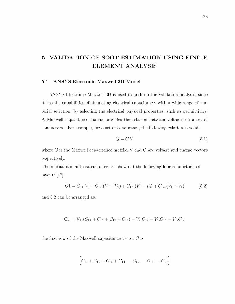
5.1 ANSYS Electronic Maxwell 3D Model
ANSYS Electronic Maxwell 3D is used to perform the validation analysis, since
it has the capabilities of simulating electrical capacitance, with a wide range of ma-
terial selection, by selecting the electrical physical properties, such as permittivity.
A Maxwell capacitance matrix provides the relation between voltages on a set of
conductors . For example, for a set of conductors, the following relation is valid:
Q = C.V (5.1)
where C is the Maxwell capacitance matrix, V and Q are voltage and charge vectors
respectively.
The mutual and auto capacitance are shown at the following four conductors set
layout: [17]
Q1 = C11.V1 + C12.(V1 − V2) + C13.(V1 − V3) + C14.(V1 − V4) (5.2)
and 5.2 can be arranged as:
Q1 = V1.(C11 + C12 + C13 + C14) − V2.C12 − V3.C13 − V4.C14
the first row of the Maxwell capacitance vector C is
[C11 + C12 + C13 + C14 −C12 −C13 −C14
]

24
Figure 5.1.: Four Conductors’ Mutual Capacitance [16]
By repeating the same derivation for Q 2, Q3, Q4, the full matrix has the form
C11 + C12+ −C12 −C13 −C14
C13 + C14
−C21 C21 + C22+ −C23 −C24
C23 + C24
−C31 −C32 C31 + C32 −C34
+C33 + C34
−C41 −C42 −C43 C31 + C32+
C33 + C34

25
5.2 Geometric Model
A geometric model of the DPF assumed to be similar to the one used at
the experimental modeling which was a cylindrical body of 6 inches diameter x 6
inches height, filter inner screen assumed to be a group of holes of 0.5 inch diameter
for its design convenience, holes distribution on the DPF’s cross-section matched
pixels layout to be reconstructed as shown at the figure 5.3 , four copper electrodes
of thickness 0.2 inches fixed around the DPF circumference, as illustrated at figure
5.2 , however the DPF design is different ,but the simulation in Ansys Electronic
assumed to be radial , and there is negligible affects.
Figure 5.2.: Diesel Particulate Filter (DPF)

26
Figure 5.3.: Pixels and Holes Distribution
5.3 Material Selection
For the DPF body a permittivity of 4.0 assigned to match the original cordierite
permittivity, for the four electrodes, copper material has been assigned, and it has a
relative permittivity of 1, a permittivity of 16.5 assigned to the soot which assumed
to be a carbon black, and air of 1.0 permittivity assigned to empty holes
Table 5.1.: Material
DPF Sensor Component Material Relative Permittivity
1 DPF body Cordierite 4
2 Electrodes Copper 1
3 Soot Carbon Black 16.5
4 Empty Holes Air 1

27
5.4 Electrodes Voltage and Solution Matrix
In case of two conducting plates , a common form is a parallel-plate
capacitor, which consists of two conductive plates insulated from each other, usually
sandwiching a dielectric material, capacitance is approximately proportional to the
surface area of the conductor plates and inversely proportional to the separation
distance between the plates. However, the definition C = Q / V does not apply
when there are more than two charged plates, or when the net charge on the two
plates is non-zero. To handle this case, Maxwell introduced his coefficients of
potential as it explained earlier in section 5.1
A charge of 5 volts applied to one of the four electrodes (source) while other
three electrodes assigned (sink) and assumed to be (0 volts) one at a time, while the
Maxwell Matrix of solution configured to be in Farads as shown in figure 5.4. A
solution matrix set up determined at Ansys pre-determined parameter to select
solution format as shown in table 5.2 and figure 5.5 respectively in capacitance
(Farad)
Figure 5.4.: Voltage of 5 Volts applied to Electrode 1

28
Table 5.2.: Maxwell solution matrix set-up
Voltage 1 Voltage 2 Voltage 3 Voltage 4
Voltage 1 x x x x
Voltage 2 x x x x
Voltage 3 x x x x
Voltage 4 x x x x
Figure 5.5.: Capacitance Solution Matrix in pF
5.5 Voltage Distribution Simulation
Voltage is the difference in electric potential between two points, is explicitly
related to the permittivity and capacitance in general as defined by equation :
C = Q / V

29
while Capacitance is the ratio of the change in an electric charge in a system to the
corresponding change in its electric potential, low permittivity, or low ability to hold a
charge, high permittivity materials are good at holding charge, they are the preferred
dielectric for capacitors.Voltage simulation shows in figure 5.6 energized electrode or
sender, voltage signal declined as it move away countered by deposited soot.
Figure 5.6.: Voltage Distribution
5.6 Sensitivity Matrix
Since the sensitivity matrix forms the foundation of the Linear Back projection
(LBP) algorithm, it should be reconstructed first, instead of Direct Techniques
method, an approach of pixel manually filling, initiated by first pixel and then
transferred to the second, and so forth until reach the 16th pixel as shown in

30
following table. In this reconstruction mode, only a single measurement data is used
independently to implement sensitivity reconstruction matrix. While in first section
study a Direct Techniques, method implemented to reconstruct the sensitivity
matrix which essentially a normalization for the capacity data took from the
inter-electrode measurement.
Table 5.3.: Sensitivity Matrix in 10−12 Farads (pF)
Pixels/Electrodes 1- 2 1- 3 1- 4 2- 3 2- 4 3- 4
1 4.8057 0.80506 4.7921 4.7349 0.75515 4.7666
2 4.9272 0.93281 5.7308 4.71 0.68944 4.6839
3 4.6799 0.69847 5.5612 4.7206 0.88917 4.9204
4 4.7357 0.75482 4.7886 4.7507 0.80433 4.8377
5 5.7558 0.93443 4.912 4.6552 0.68784 4.7379
6 4.8442 0.91986 4.8699 4.6532 0.84478 4.7209
7 4.6692 0.84448 4.8599 4.6764 0.91994 4.9127
8 4.6473 0.68803 4.9383 4.6243 0.92913 5.7154
9 5.7398 0.68844 4.6378 4.9259 0.93282 4.7327
10 4.8412 0.84467 4.6807 4.8318 0.91927 4.6792
11 4.6089 0.91778 4.6356 4.7651 0.83963 4.8024
12 4.5688 0.9272 4.5379 4.8032 0.68039 5.6469
13 4.8036 0.75627 4.7169 4.8025 0.80369 4.7663
14 4.9248 0.68909 4.6928 5.7536 0.93247 4.6807
15 4.6549 0.93333 4.6919 5.7558 0.68721 4.9516
16 4.7363 0.8047 4.7169 4.8034 0.7553 4.8306
Empty DPF 4.7466 0.77929 4.7275 4.8119 0.77768 4.8153
Full DPF 8.1929 1.8334 8.1873 8.3072 1.8309 8.3224

31
5.7 Capacitance Data Collection
Two methods were adapted to obtain capacitance data from the inter-electrode
excitation, the first was the random distribution and the other was circumferentially
distributed soot inside DPF, where 3 holes filled initially from the center of DPF,
and then incremented by 3 holes in spiral order until the DPF was fully filled, as we
know the fundamental of ECT known as: different materials with different permit-
tivities. If the concentration and the composition of the components are changed,
the permittivity will change cross the DPF sensor, as a result this contrast in per-
mittivity will cause a change of the capacitance measurements, for this reason, a
randomly distributed soot inside the filter basically will test the real-life scenario,
moreover, simulation data will give more opportunities to explore and analyze results
and method.

32
Table 5.4.: Random Filling Distribution in 10−12 Farads (pF)
No. of holes filled/Electrodes 1 − 2 1 − 3 1 − 4 2 − 3 2 − 4 3 − 4
3 4.6337 0.75532 4.8746 4.605 0.80653 4.9252
6 4.7519 0.77502 5.6992 4.6337 0.81404 4.8839
9 4.8962 0.8525 5.8664 4.6646 0.75152 4.9086
12 4.9844 0.96563 6.2696 4.5743 0.78424 4.8546
15 5.002 0.93488 7.5725 4.5257 0.81393 4.9051
18 5.1038 0.91989 8.1212 4.5741 0.88125 5.0862
21 5.2064 1.0035 8.2019 4.5123 0.98415 5.3704
24 5.1749 1.0413 8.4071 4.4809 1.1035 5.8656
27 6.2277 1.1204 8.5123 4.4509 1.1089 5.835
30 7.2335 1.1769 8.4064 4.4942 1.3098 5.9442
33 7.2661 1.3763 8.3062 4.6056 1.3314 7.2451
36 7.2107 1.5684 8.2823 4.7106 1.4247 7.3622
39 7.1944 1.7966 8.155 4.9452 1.3844 7.9849
42 7.957 1.6654 8.028 5.1722 1.5803 7.9456
45 8.0791 1.7069 7.9668 5.671 1.7318 7.9229
52 8.1929 1.8334 8.1873 8.3072 1.8309 8.3224

33
Table 5.5.: Normalized Sensitivity Matrix
0.98 0.98 0.98 1.02 1.02 1.01
0.95 0.85 0.71 1.03 1.08 1.04
1.02 1.08 0.76 1.03 0.89 0.97
1.00 1.02 0.98 1.02 0.97 0.99
0.71 0.85 0.95 1.04 1.09 1.02
0.97 0.87 0.96 1.05 0.94 1.03
1.02 0.94 0.96 1.04 0.86 0.97
1.03 1.09 0.94 0.00 0.86 0.74
0.71 1.09 1.03 0.97 0.85 1.02
0.97 0.94 1.01 0.99 0.87 1.04
1.04 0.87 1.03 1.01 0.94 1.00
1.05 0.86 1.05 1.00 1.09 0.76
0.98 1.02 1.00 1.00 0.98 1.01
0.95 1.09 1.01 0.73 0.85 1.04
1.03 0.85 1.01 0.73 1.09 0.96
1.00 0.98 1.00 1.00 1.02 1.00

34
5.8 Circumferential Distributed Soot
Soot filled in DPF with one pattern, starting from the center and increasingly
by three holes at a time spirally toward the DPF external circumference. This
distribution will give more insights to explore dielectric distribution behavior and its
contribution to the determining the mutual capacitance and eventually its effects on
the gray-level value.
Table 5.6.: Circumferential Filling Distribution in 10−12 Farads (pF)
No. of holes filled/Electrodes 1- 2 1- 3 1- 4 2- 3 2- 4
3 4.7083 0.89101 4.7439 4.7136 0.87617
6 4.7974 0.97461 4.7242 4.7812 0.9763
9 4.9498 1.0765 4.9358 4.7293 1.0347
12 4.8856 1.1408 5.0349 4.74 1.1398
15 4.8929 1.2666 4.9736 4.8953 1.1947
18 5.2454 1.2224 4.9132 5.0942 1.3672
21 5.7754 1.4039 5.136 5.0117 1.2818
24 5.9007 1.5096 5.4308 4.9748 1.2499
27 5.8096 1.3856 5.8374 4.9049 1.4571
30 5.7559 1.5113 5.8226 5.0007 1.4741
33 5.6825 1.723 5.4704 5.4099 1.3925
36 5.9799 1.6304 5.6709 5.9733 1.5897
39 7.713 1.5962 5.6622 6.1422 1.713
42 8.2973 1.8194 6.492 6.0499 1.5411
45 8.1707 1.6566 7.9332 5.9806 1.7671
52 8.1929 1.8334 8.1873 8.3072 1.8309

35
6. ANSYS’S IMAGES AND COMPUTATIONAL
RESULTS
6.1 Soot Estimation Method using ANSYS Images
Based on chapter 5 material, ECT images were generated from ANSYS
modeling using LBP.The following images represent randomly filled holes of the
DPF. As it can be observed from figure 6.1.a which has 36 filled holes, 6.1.b has 18
filled holes, 6.1.c has 12 filled holes, and 6.1.d has 3 filled holes. Gray-level varied
from 36 filled holes down to 3 filled holes.
(a) 36 filled holes. (b) 18 filled holes.
(c) 12 filled holes. (d) 3 filled holes.
Figure 6.1.: Randomly Distributed and filled holes.

36
6.2 Images (Gray-Level)- Circumferential Distributed Soot
From the simulation results a numerical sum of vector [K] obtained as shown in
LBP equation:
[K] = [S]T .[C]
While filled soot amount inside the DPF (Maxwell model) calculated using carbon
black physical, and geometrical properties. Similar calculation method explained at
section (3.1), a numerical sum of the gray-level [K] vector assumed to be related to
the deposited soot. The numerical sum of [K] represents the gray-level value used
to estimate the filled soot, for both Random and circumferential soot filling
arrangement, a non-linear polynomial equation derived using excel curve fitting
tools, polynomial equation (4.1)
y = a1x6 + a2x
5 + a3x4 + a4x
3 + a5x2 + a6x+ a
Using curve fitting tools in MS Excel a1 , a2 , a3 , a4 , a5 , and a6 can be located
respectively as below:
1− Random Distribution
y = (−5E − 07)x5 + (6E − 05)x4 − 0.0028x3 + 0.0502x2 − 0.5295x+ 17.406
where y estimated number of holes filled, and x is gray level value. Polynomial
equation coefficients a1, a2, a3, a4, a5, and a6 are :
a1 = 1.52118E − 05 , a2 = −0.000550069 , a3 = 0.003228188
a4 = 0.076203506, a5 = −1.078575735, a6 = 1.616596238
2− Circumferential Distribution:
y = −0.0002x6 + 0.0109x5 − 0.2395x4 + 2.5302x3 − 12.891x2 + 23.73x + 51.998
Polynomial equation coefficients a1, a2, a3, , a4, a5, anda6are :
a1 = −0.000191585, a2 = 0.010889287, a3 = −0.239540012
a4 = 2.530212898, a5 = −12.89055524, a6 = 23.72970661
a = 0

37
Figure 6.2.: Randomly Distributed Soot
Figure 6.3.: Circumferential Distributed Soot

38
Table 6.1.: Nos. of filled holes vs Gray-Level Random Distribution
Gray-Level Value Actual Weight Estimated Weight Error %
No of Filled Holes (No of holes)
1 16.15794723 3 2.907553055 -3.081564835
2 15.5001599 6 6.847677051 14.12795085
3 15.21758948 9 8.498537666 -5.571803715
4 14.74457232 12 11.16428706 -6.964274527
5 13.94898682 15 15.29055728 1.93704853
6 13.23313331 18 18.56450207 3.136122635
7 12.58396253 21 21.17123573 0.815408251
8 11.8198292 24 23.84135302 -0.661029066
9 10.94508015 27 26.47594141 -1.94095774
10 9.650045982 30 29.88222004 -0.392599871
11 8.154963213 33 33.69012893 2.091299794
12 7.36324128 36 35.8512668 -0.413147777
13 6.310931613 39 38.96986668 -0.077264935
14 5.473303797 42 41.63196323 -0.876278023
15 4.376593173 45 45.20785969 0.461910421
16 0 52 51.996 -0.007692308

39
Table 6.2.: Circumferential Distribution Estimated Weight
Gray-Level Value Actual Weight No of Filled Error %
Holes
1 15.691 3 3.06 1.908
2 15.187 6 6.07 1.203
3 14.666 9 8.89 -1.249
4 14.146 12 11.61 -3.250
5 13.511 15 14.97 -0.224
6 12.814 18 18.74 4.132
7 12.271 21 21.70 3.336
8 11.926 24 23.55 -1.878
9 11.408 27 26.22 -2.887
10 10.607 30 29.97 -0.092
11 9.859 33 32.90 -0.296
12 8.632 36 36.42 1.168
13 7.130 39 39.41 1.056
14 6.318 42 41.24 -1.812
15 5.159 45 45.25 0.559
16 0.000 52 52.00 -0.004

40
Table 6.3.: Random vs Circumferential Distribution (Errors)
Estimated Weight Estimated weight Circular-Error % Random - Error %
Circular Random
3.06 2.91 1.91 -3.08
6.07 6.85 1.20 14.13
8.89 8.50 -1.25 -5.57
11.61 11.16 -3.25 -6.96
14.97 15.29 -0.22 1.94
18.74 18.56 4.13 3.14
21.70 21.17 3.34 0.82
23.55 23.84 -1.88 -0.66
26.22 26.48 -2.89 -1.94
29.97 29.88 -0.09 -0.39
32.90 33.69 -0.30 2.09
36.42 35.85 1.17 -0.41
39.41 38.97 1.06 -0.08
41.24 41.63 -1.81 -0.88
45.25 45.21 0.56 0.46
52.00 52.00 0.00 -0.01
6.3 Ansys Validation and Results and Discussion
Capacitance measurements obtained from inter-electrode data, forms a direct
relationship between capacitance and material deposited inside the DPF, this form
exhibits proportional relationship, in-line with the assumption of more soot deposited
results in more capacitance,although,The capacitance of a set of charged parallel
plates is increased by the insertion of a dielectric material. The capacitance is in-
versely proportional to the electric field between the plates, and the presence of the

41
dielectric reduces the effective electric field. on other hand capacitance is following
direct proportional of soot mass contribution at the time capacitances were measured.
In Validation process two pattern of soot mass deposition implemented, random
soot distribution,and circumferential soot distribution,in order to explore and ob-
serve the behavior of simulation results, from the charts there were slight difference,
the errors in circumferential tends to be less than ±5%, while random distribution’s
exceeded errors acceptable range in three points, these spikes attributed to some lim-
itation in Ansys electronic desktop where no feature to electrically ground electrodes,
besides, the difficulty of transforming DPF circular shape into square pixel domain.
Results as illustrated in figures circumferential distribution showed the best re-
sults, however in real time estimation method should apply for all situation.
Figure 6.4.: Random Distribution Error%
The estimation errors for the case with DPF holes filled randomly are plotted in
figure 6.4.; a maximum error of 14% is observed.

42
Figure 6.5.: Circumferential Distribution -Actual Nos of holes filled vs Estimated
.
The estimation errors for the case with DPF holes filled circumferentially as shown
in figure 6.5; estimation errors were in the acceptable range of maximum 4%.
Figure 6.6.: Random vs Circumferential Distribution
Soot weight estimation patterns were plotted as shown in figure 6.6. A close match
between random and circumferential distribution, based on the number of filled
holes was observed.

43
Figure 6.7.: Random vs Circumferential Distribution Errors
Figure 6.7 shows the soot estimation errors for soot distributed randomly and
circumferentially.

44
7. CONCLUSION AND FUTURE WORK
7.1 Conclusion
The aim of the presented work was to estimate soot mass from generated ECT
image’s data. Sensitivity matrix for an ECT image forms a basis set from which
image pixel data can be obtained. In this research, an approach is presented to es-
timate the soot mass in a Diesel Particulate Filter from an ECT image utilizing its
permittivity (capacitance) data, and then making use of pixel’s gray-level data for
estimation process .MATLAB software was used as a tool for processing the digital
image data, and generating numerical values, for both experimental and validation
portions. The proposed approach was evaluated for its accuracy against actual soot
mass and its corresponding tomographic images data. The results obtained by com-
bining the pixel value with soot load physical properties (weight) and permittivity
parameters (capacitance) through nonlinear relationship showed reasonable accuracy
in estimating the actual soot mass. Moreover it has been observed from the ex-
perimental data and validation results , soot estimation computation and analysis
showed that voltage is proportional to deposited soot weight, while capacitance data
used in simulation displayed inversely proportional relationship between number of
holes filled with soot. This results coincide with the basic definition of relationship
between charge ,voltage , and capacitance , and proves that experimental and val-
idation results are on the right track, however there are small estimation errors in
the results but they are controllable by enhancing sensor electrode and procedures in
experimental data collection.

45
(a) Voltage vs Estimated Soot. (b) Capacitance vs Estimated Soot.
Figure 7.1.: Voltage fill-in data vs Gray-Level (Experimental), and Capacitance fill-in
data vs Gray-Level (validation).
7.2 Future Work
Controlling the soot mass deposition / emission level in the diesel engines ex-
haust system is a crucial process for manufacturers and environmental regulators.
Several studies have been conducted to figure out this problem using experimental,
analytical, and numerical approaches, however there are some challenges still need
further investigations. Based on the conclusions drawn from the study performed
herein, the following concerns can be basis for future work to advance improvement
in this area.
1- The ANSYS software used in this study to create a finite element model of the
diesel particulate filter (DPF) does not include a function for the electrical ground
system. This resulted in spikes on capacitance reading which impacted the accuracy
and linearity of the field distribution. Technically, the negligence of the electrical
ground system leads to residual accumulation and flow of the electrical field which
eventually impacts sensor’s electrodes mutual capacitance .
2- The sensitivity matrix used in this study as tools /techniques to quantify the soot
mass accumulation can be improved by weighing more geometric models capable of
transforming circular cross-section of the filter outer shell into square pixel grid , as it

46
assumed a full size of the outer pixels during the data transformation into a sensitivity
matrix. This assumption slightly affects the accuracy of the sensitivity’s matrix .
3- Two approaches implemented to generate sensitivity matrix , Direct technique and
Manual deposition , other approaches could be tried to improve the quality of the
images generated as well.

REFERENCES

47
REFERENCES
[1] R. Huq and S. Anwar, “Real-time soot measurement in a diesel particulate filter,”US Patent 9,151,20, 2015.
[2] Du, Yanting, H. Guangdi, X. Shun, Z. Ke, L. Hongxing, and G. Feng,“Estimation of the diesel particulate filter soot load based on an equivalentcircuit model”. Energies, vol. 11, no. 2, 2018.
[3] G. Ramon. “after-treatment systems DPF (Diesel Particulate Filter)”.[Online]. Available: http://www.drawfolio.com/en/portfolios/ramongarcia-gonzalez/picture/50223picture-navigation
[4] W. Wade, “Diesel particulate trap regeneration techniques”. SAE TechnicalPaper 810118, 1981.
[5] P. Chen and J. Wang, “Control-oriented model for integrated diesel engine andaftertreatment systems thermal management”. Control Eng. Pract., vol. 22,pp.81-93, 2014.
[6] E. Alhosani, Electrical capacitance tomography for real-time monitoring of pro-cess pipelines . A thesis submitted for the degree of Doctor of Philoso-phy,University of Bath Department of Electronic Electrical Engineering, 2016.
[7] M. Zhang, Permittivity and Conductivity Imaging in Electrical Capacitance To-mography . The thesis submitted for the degree of Doctor of Philosophy ,TheDepartment of Electronic and Electrical Engineering University of Bath g, 2015.
[8] Q. Marashdeh, “Advances in Electrical Capacitance Tomography”. The OhioState University: MS Thesis, 2006.
[9] A. Jaworski and T. Dyakowski, “Application of electrical capacitance tomogra-phy for measurement of gas–solid flow characteristics in a pneumatic conveyingsystem”. Measurement Science and Technology, vol. 12, pp 1109, 2001.
[10] T. Masturah, R. M, Z. Zulkarnay, R. A, and N. M. Ayob, “Design of FlexibleElectrical Capacitance Tomography Sensor”. Jurnal Teknologi, vol. 77, no. 28,2015.
[11] Soleimani, Manuchehr, and L. William, RB, “Nonlinear image reconstructionfor electrical capacitance tomography using experimental data”. Reading Mas-sachusetts: Measurement Science and Technology , vol. 16, no. 10, pp 1987–1996,2005.
[12] R. White, “Using electrical capacitance tomography to monitor gas voids in apacked bed of solids”. Meas. Sci.Technol ,vol. 13,pp. 1842–1847, 2002.
48
[13] A. Brahma, “Modeling and Observability Analysis of DPF Regeneration”. AnnArbor, USA: ASME 2008 Dynamic Systems and Control Conference, 2008.
[14] Y. W, Q and P. Lihui, “ Image reconstruction algorithms for electrical capaci-tance tomography”. Measurement Science Technology, 2003.
[15] M. Huang, A. Plaskowski, C. Xie, and M. Beck, “Capacitance-based tomo-graphic flow imaging system”. Electronics letters, vol. 24, no. 7, pp. 418-419,1988.
[16] A. Kowalska, B. Robert, W. Rados law, R. Andrzej, and D. Sankowski, “Towardshigh precision electrical capacitance tomography multi-layer sensor structure us-ing 3D modelling and 3D printing method”. International Interdisciplinary PhDWorkshop (IIPhDW), pp. 238-243. IEEE, 2018.
[17] W. Paper, The Maxwell Capacitance Matrix. White Paper WP110301, 2011.