Some History and Research of Frank

Stenger

*******

1 The Earlier Years.

Frank Stenger was born in Magyarpolany, Hungary, on July 6, 1938. Hisparents were Stenger Gyorgy and Gorgy Katalin. An historical check showsthat his motherGorgy Katalin’s ancestors were already present in Hungaryin the early 1600’s, whereas the Stenger side of the family came to Hungaryin 1750, following the forced retreat of the Turks out of Hungary, by theHapsburgs.

Both of Frank’s grandparents, Gyorgy Miska and Stenger Simon fought inWWI; Gyorgy Miska was killed in that war, whereas Stenger Simon lost aleg and the use of an arm. Frank’s father, Stenger Gyorgy, spent nearlyten years conscripted by the Hungarian army preceding and during WWII.Indeed, he was one of the very few that survived after being captured onthe Russian Front.

Magyarpolany was primarily a German speaking town, with a German di-alect close to that of the street language of Vienna, although Hungarian wasspoken equally often in the house in which Frank Stenger (who was calledStenger Ferenc in Hungary) lived since birth.

Frank Stenger’s family was well off before the end of WWII, but they losttheir home and all of their properties shortly after the end of that war.Frank, his sister, Kati (4 years younger than Frank) and his father andmother were forced to live with relatives, in cramped quarters, and in orderto survive, they stole vegetables from the garden that they had previouslyplanted on their former property.

In 1947 most of the people of Magyarpolany were ethnically cleansed out of

1

Hungary. They were locked into box cars and shipped off to East Germany.After spending 5 weeks in a refugee camp, the Stenger family was forced tolive in the downstairs area of an older couple’s house, in Zwonitz, Erzgb.Sachsen, East Germany. Whereas they were used to having plenty to eatin Hungary, food was scarce in East Germany at that time. For this, andfor other reasons, after spending less than one year in East Germany, theysneaked over the border to West Germany. They lived in Braunschweig forabout a year, after which Frank’s uncle, who had moved to Alberta over 10years earlier, arranged for them to come to Canada. They spent the firstyear in Warburg, Alberta, picking roots on Frank’s uncle’s farm, to pay backthe money it cost his uncle to bring them to Canada.

Frank’s father then bought a farm. He was, however, unlucky with crops:at the end of the first year of planting, all of the crops were lost due to hail;there was too much rain during the second year, which killed the crops; andthe snow came too early in the third year, making it impossible to removethe crops in time, and as a result, they were eaten by mice over the winter. Itwas then that Frank decided that if he wanted to get an education, he wouldhave to do it on his own. Consequently, he supported himself by winningscholarships, and fellowships and with excellent job opportunities until theend of his Ph.D. studies. His teachers, too, especially his high school mentorErwin Stobbe, and his University of Alberta mentor, J.J. McNamee playedimportant roles in these decisions.

Frank’s sister, Kati (called Katherine in Canada) also did well scholasti-cally. The two younger brothers, George and Edward, who were born inCanada did well monetarily, although they were less interested in scholasticachievements.

Frank owes a great deal for his education and academic career to:

His mother – for her many life-long sacrifices for him; His excellent teachers,

especially to his “Big Brother”, Ervan Stobbe who started Frank’s love ofmathematics; and His mentor, John McNamee.

Frank enrolled in the electrical engineering program at the University of Al-berta. While at residence, he met an Irish mathematician, John McNamee,who decided that Frank had some mathematical ability, and who gave Franka copy of R. Courant’s two-volume calculus texts. It did not take Frank longto solve all of the problems of these texts, which, in effect, sealed his fate

2

in mathematics. After completion of his bachelor’s degree in EngineeringPhysics, Frank enrolled in two simultaneous Master’s degree programs, inMath. (Numerical Analysis, with specialty of n-dimensional quadratures),and in Engineering (Control Theory, with specialty of nonlinear controls).Although he completed the work of each, he only did a final oral and formalcompletion in his numerical analysis masters. He then did a Ph.D. degreein Math (Asymptotics), after spending a year at the National Bureau ofStandards in Washington, D.C. His official Ph.D. adviser at the Univ. ofAlberta Dept. of Math. was Ian Whitney, an expert in complex variables,who had previously worked with A. Erdelyi on the Bateman manuscriptprojects, and from whom Frank Stenger learned a great deal about analyticfunctions, including elliptic functions.

2 Some Research Results of Frank Stenger.

Only some of the research of Frank Stenger is touched upon in this report.There is, however, an (roughly) 80% complete set of references at the endof this report. Sinc related research of Frank Stenger is covered in thefirst subsection below. This is then followed by inverse problems research,miscellaneous research results, program packages, and textbooks.

2.1 Sinc Related Research of Frank Stenger.

1. In 1964, John McNamee and Ian Whitney wrote a joint paper, “Whit-taker’s Cardinal Function in Retrospect”, which they submitted to SIAM.Unfortunately they had an incompetent referee, who made many unfair crit-icisms of their paper. They were, however proud men, and refused to rewritetheir paper. McNamee gave a copy of this paper to Frank Stenger, and afterreading it for the third time, Frank got quite excited about it. He approachedMcNamee and Whitney — offering to to rewrite the paper, by incorporat-ing the two reasonable suggestions the referee had made, and also, to makesome improvements, e.g., the inclusion of the Paley–Wiener theorem, moreexamples, as well as some applications — and if he did this, would they lethim become a joint author. They agreed, and with this publication [16] theCardinal function

3

C(f, h)(x) =∞∑

k=−∞

f(k h)S(k, h)(x)

S(k h)(x) = sinc

(

x

h− k

)

sinc(x) =sin(π x)

π x,

(1)

became a big part of Frank Stenger’s approach to computation. Here, sinc(x)is the sinc function coined so by engineers, while we shall refer to the func-tions S(k, h) as Sinc functions. The beautiful coinage of this function inthe original paper (most likely due to McNamee) was “... a function ofroyal blood, whose distinguished properties separate it from its bourgeoisbrethren”.

2. After his Ph.D. work, he spent 1965–66 in the Computer Science Depart-ment at the University of Alberta, In the fall of 1966, he joined the Mathe-matics Department at the University of Michigan as an Assistant professor,where he concentrated primarily on improving his mathematical skills. Atthat time, there were over 20 seminars held in the department each week,and he attended 11 of these. One of the themes of the department involvedvarious aspects of the Wiener-Hopf process: the applied mathematicianswere solving Wiener–Hopf problems; the functional analysts were factoringToeplitz operators; the approximation group was studying approximationby rations of analytic functions; and the probabilist were studying discreteWiener–Hopf equations. In particular, during that time, Ron Douglas andWalter Rudin wrote a joint paper, proving that: Given function f ∈ L∞(T ) ,with T the unit circle, given any ε > 0, there exists a positive integer n ,inner functions (functions that are analytic and unimodular in the unit discU) ϕ1 , ψ1 , . . . ϕn , ψn and constants c1 , . . . , cn such that

ess sup

r → 1−

∣

∣

∣

∣

∣

∣

f(

ei θ)

−n∑

j=1

cjϕj

(

r ei θ)

ψj (r ei θ)

∣

∣

∣

∣

∣

∣

< ε (2)

a.e.

Stenger [17] gave a constructive proof of this result, showing moreover, thatthe approximation can be accomplished with n = 2 . In his proof, Stenger

4

constructed a novel elliptic function, which was an approximate character-istic function on a measurable set. Shortly afterward, while visiting theUniversity of Montreal in 1970, he reconstructed a variant of this beautifulfunction in great detail [38], based on a geometric-analytic function proof,via use of elliptic functions. Indeed, Stenger considers [38] to be his firstSinc methods paper, which led him to the development of the area of Sinccomputation. In the same paper, [38] he disproved a conjecture made earlierby several others, which we now describe. In 1965 [130], H.S. Wilf posedthe problem, to determine the best σ(n), with

σ(n) =

infwj∈ lC, zj∈U

supf∈H2(U),‖f‖=1

∣

∣

∣

∣

∣

∣

∫ 1

−1f(x) dx−

n∑

j=1

wj f(xj)

∣

∣

∣

∣

∣

∣

,(3)

where H2(U) is the Hardy space of all functions f that are analytic on theunit disc U , normed by

‖f‖ =

(

limr→1−

∫ 2 π

0

∣

∣

∣f(

r ei θ)∣

∣

∣

2dθ

)1/2

.

In his paper [130], Wilf obtained

σ(n) = O(

(

log(n)

n

)1/2)

.

Shortly thereafter there followed three independent research articles, eachof which obtained the estimate σ(n) = O(n−1/2): by S. Haber (in Quart.Appl. Math., 29 (1971) 41-420), by Johnson & Riesz (University of TorontoResearch Report) and S. Ecker (Ph.d. thesis, University of Hamburg) andwith each independently making the conjecture that this is the best bound

possible. Stenger got σ(n) = O(

exp(

−π (n/2)1/2))

, via use of an explicit

“q–series” type quadrature formula constructed in [38] .In [38]1 Stenger obtained several explicit q-series–type quadrature formulasvia transformations of simple conformal maps in the characteristic functionhe constructed: (i) an arc of the unit circle, (ii) the interval (−1, 1), (iii) theinterval (0,∞) , and (iv) the real line lR = (−∞ ,∞) . The latter was just

1The publication of this paper came much later than its discovery. After the referee ofthe journal it was submitted to kept it for over a year, he recommended turning it down.

5

the trapezoidal rule, but with nearly the exact same bound on the error thatwas previously obtained in [16]. This connection with the above Cardinalseries led his mentor, J. McNamee, to suggest to Stenger that he should usethis Cardinal series rather than elliptic functions to derive such formulas,since the Cardinal series would be understood by a wider audience.

3. As a visitor to the Univ. of British Columbia during the academic yearof 1975–76, Stenger applied various conformal maps to the series (1), toget explicit, accurate Sinc–type methods for approximation over arbitraryintervals and contours [34].

4. Whenever the series (3) above converges, the resulting function is anentire function of order 1 and type π/h . If f is also an entire function of order1 and type π/h that is uniformly bounded on lR , then the function C(f, h)defined in (1) above satisfies the identity C(f, h) = f . In this space thefunction C(f, h) is replete with many identities obtained via operations onC(f, h), such as differentiation, orthogonality, delta function-like behavior ofSinc functions, Fourier transforms, Hilbert transforms, etc. These identitiesbecome highly accurate approximations if f is not analytic in the entirecomplex plane, but rather, analytic and uniformly bounded only in the strip

Dd = z ∈ lC : |ℑ(z)| < d ,a region which arose naturally in the derivation of the quadrature rules of[38]. A conformal map ϕ of another region

D = z ∈ lC : | arg(ϕ(z))| < donto Dd automatically yields methods of interpolation (as well as otherformulas of approximation) over a contour Γ = ϕ−1(lR), of the form

F ≈ C(F, h) ϕ =∞∑

k=−∞

F (zk)S(k, h) ϕ ,

∫

ΓF (x) dx ≈

∫

ΓC(F, h) ϕ(x) dx ≈ h

∞∑

k=−∞

F (zk)

ϕ′(zk).

(4)

with zk = ϕ−1(k h) denoting the Sinc points. Moreover, those same identi-ties for the function C(f, h) now still hold, and one gets exactly the samebounds on the errors of approximation. In this way, we get an explicit family

6

of formulas for interpolation, quadrature, differentiation, and Hilbert trans-forms, ..., etc., for arbitrary bounded, semi–infinite, infinite intervals andeven for analytic arcs.

For example: If ϕ(z) = log(z) , then D is the sector, | arg(z)| < d , theinterval Γ = (0,∞) , the Sinc points are zk = ekh , the “weights”, h/ϕ′(zk) =h ekh;

If ϕ(z) = log(z/(1 − z)) , then D is the “eye-shaped” region (see [4], p. 68,for a picture), | arg(z/(1−z))| < d , the interval Γ = (0, 1) , the Sinc pointsare zk = ekh/(1 + ekh) , the “weights”, h/ϕ′(zk) = h ekh/(1 + ekh)2 .

5. The concept of Sinc spaces was formulated somewhat later (in 1984).An understanding of these spaces enable one to tell a priori when one canachieve uniform accuracy over Γ via use of Sinc methods, by means of arelatively small number of points. (Actually, because the Sinc methods ap-proximate functions at Sinc points – all of which are in the interior of Γ –they achieve approximations that are accurate to within a relative error evenwhen they approximate an operation the result of which is unbounded at anend point of Γ . This occurs e.g., for differentiation, for Laplace transform in-version, for the approximation of Hilbert transforms, for the approximationof Abel–type integrals, etc.) It is convenient to introduce the Sinc spaces atthis time.

Along with the conformal map ϕ of D to Dd , we set ρ = exp(ϕ), we denotethe end points of Γ = ϕ−1(lR) by a = ϕ−1(−∞) and b = ϕ−1(∞) , weassume that F is analytic and bounded in D , and that limiting values F (a)and F (b) exist, so that the expression

LF =F (a) + ρF (b)

1 + ρ(5)

is well defined. (Note that as traverses Γ from a to b , ρ(z) is real valued,and increases strictly from 0 to ∞ .) We then say that

A. F ∈ Lα,d(ϕ) if there exist positive constants C and α such that |F (z)| <C exp(−α |ϕ(z)|) for all z ∈ D .

B. F ∈ Mα,d(ϕ) if F − LF ∈ Lα,d(ϕ) .

Let us also introduce the Hilbert and Cauchy transforms:

7

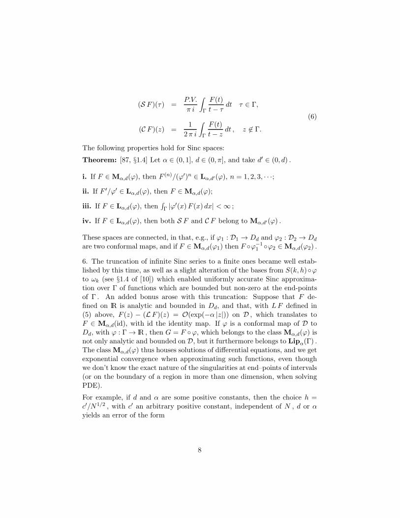
(S F )(τ) =P.V.

π i

∫

Γ

F (t)

t− τdt τ ∈ Γ,

(C F )(z) =1

2π i

∫

Γ

F (t)

t− zdt , z 6∈ Γ.

(6)

The following properties hold for Sinc spaces:

Theorem: [87, §1.4] Let α ∈ (0, 1], d ∈ (0, π], and take d′ ∈ (0, d) .

i. If F ∈ Mα,d(ϕ), then F(n)/(ϕ′)n ∈ Lα,d′(ϕ), n = 1, 2, 3, · · ·;

ii. If F ′/ϕ′ ∈ Lα,d(ϕ), then F ∈ Mα,d(ϕ);

iii. If F ∈ Lα,d(ϕ), then∫

Γ |ϕ′(x)F (x) dx| <∞ ;

iv. If F ∈ Lα,d(ϕ), then both S F and C F belong to Mα,d′(ϕ) .

These spaces are connected, in that, e.g., if ϕ1 : D1 → Dd and ϕ2 : D2 → Dd

are two conformal maps, and if F ∈ Mα,d(ϕ1) then F ϕ−11 ϕ2 ∈ Mα,d(ϕ2) .

6. The truncation of infinite Sinc series to a finite ones became well estab-lished by this time, as well as a slight alteration of the bases from S(k, h)ϕto ωk (see §1.4 of [10]) which enabled uniformly accurate Sinc approxima-tion over Γ of functions which are bounded but non-zero at the end-pointsof Γ . An added bonus arose with this truncation: Suppose that F de-fined on lR is analytic and bounded in Dd, and that, with LF defined in(5) above, F (z) − (LF )(z) = O(exp(−α |z|)) on D , which translates toF ∈ Mα,d(id), with id the identity map. If ϕ is a conformal map of D toDd, with ϕ : Γ → lR , then G = F ϕ, which belongs to the class Mα,d(ϕ) isnot only analytic and bounded on D, but it furthermore belongs to Lipα(Γ) .The class Mα,d(ϕ) thus houses solutions of differential equations, and we getexponential convergence when approximating such functions, even thoughwe don’t know the exact nature of the singularities at end–points of intervals(or on the boundary of a region in more than one dimension, when solvingPDE).

For example, if d and α are some positive constants, then the choice h =c′/N1/2 , with c′ an arbitrary positive constant, independent of N , d or αyields an error of the form

8

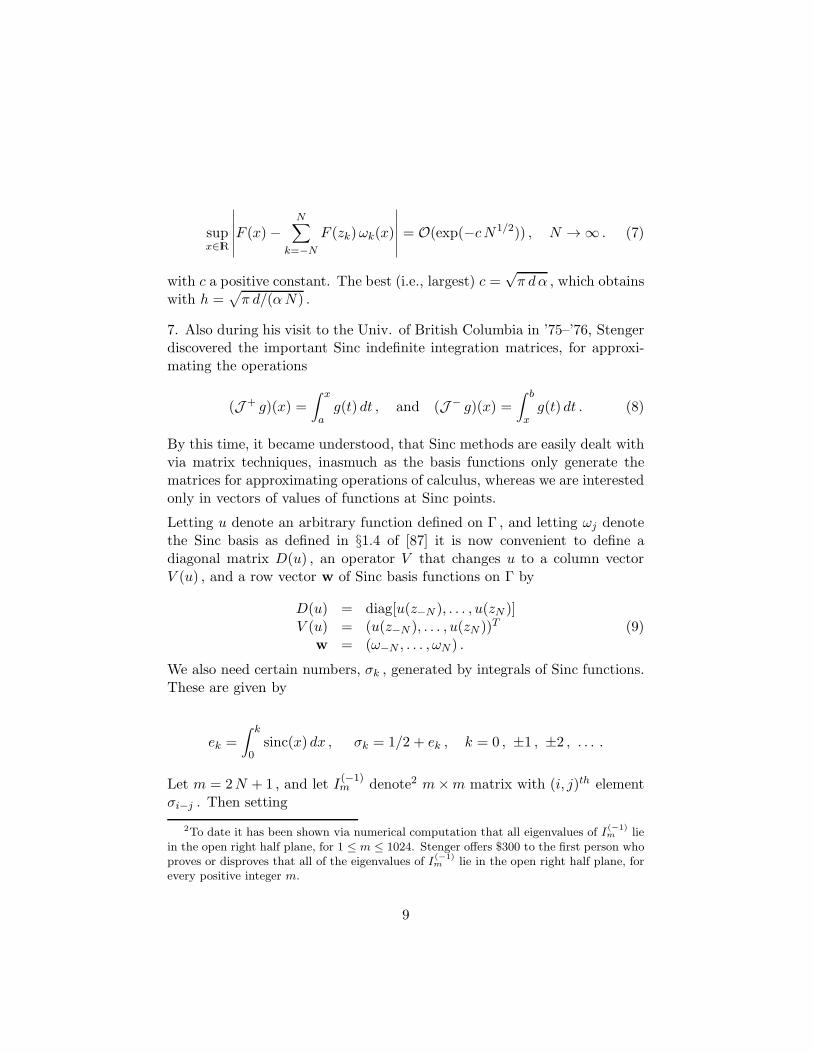
supx∈lR

∣

∣

∣

∣

∣

∣

F (x)−N∑

k=−N

F (zk)ωk(x)

∣

∣

∣

∣

∣

∣

= O(exp(−cN1/2)) , N → ∞ . (7)

with c a positive constant. The best (i.e., largest) c =√π dα , which obtains

with h =√

π d/(αN) .

7. Also during his visit to the Univ. of British Columbia in ’75–’76, Stengerdiscovered the important Sinc indefinite integration matrices, for approxi-mating the operations

(J + g)(x) =

∫ x

ag(t) dt , and (J − g)(x) =

∫ b

xg(t) dt . (8)

By this time, it became understood, that Sinc methods are easily dealt withvia matrix techniques, inasmuch as the basis functions only generate thematrices for approximating operations of calculus, whereas we are interestedonly in vectors of values of functions at Sinc points.

Letting u denote an arbitrary function defined on Γ , and letting ωj denotethe Sinc basis as defined in §1.4 of [87] it is now convenient to define adiagonal matrix D(u) , an operator V that changes u to a column vectorV (u) , and a row vector w of Sinc basis functions on Γ by

D(u) = diag[u(z−N ), . . . , u(zN )]V (u) = (u(z−N ), . . . , u(zN ))T

w = (ω−N , . . . , ωN ) .(9)

We also need certain numbers, σk , generated by integrals of Sinc functions.These are given by

ek =

∫ k

0sinc(x) dx , σk = 1/2 + ek , k = 0 , ±1 , ±2 , . . . .

Let m = 2N + 1 , and let I(−1)m denote2 m×m matrix with (i, j)th element

σi−j . Then setting

2To date it has been shown via numerical computation that all eigenvalues of I(−1)m lie

in the open right half plane, for 1 ≤ m ≤ 1024. Stenger offers $300 to the first person whoproves or disproves that all of the eigenvalues of I

(−1)m lie in the open right half plane, for

every positive integer m.

9

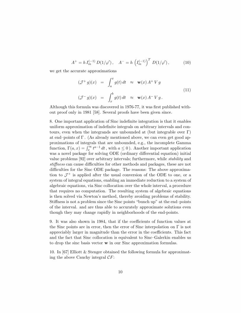
A+ = h I(−1)m D(1/ϕ′) , A− = h

(

I(−1)m

)TD(1/ϕ′) , (10)

we get the accurate approximations

(J+ g)(x) =

∫ x

ag(t) dt ≈ w(x)A+ V g

(J− g)(x) =

∫ b

xg(t) dt ≈ w(x)A− V g .

(11)

Although this formula was discovered in 1976-77, it was first published with-out proof only in 1981 [58]. Several proofs have been given since.

8. One important application of Sinc indefinite integration is that it enablesuniform approximation of indefinite integrals on arbitrary intervals and con-tours, even when the integrands are unbounded at (but integrable over Γ)at end–points of Γ . (As already mentioned above, we can even get good ap-proximations of integrals that are unbounded, e.g., the incomplete Gammafunction, Γ(a, x) =

∫∞x ta−1 dt , with a ≤ 0 ). Another important application

was a novel package for solving ODE (ordinary differential equation) initialvalue problems [92] over arbitrary intervals; furthermore, while stability andstiffness can cause difficulties for other methods and packages, these are notdifficulties for the Sinc ODE package. The reasons: The above approxima-tion to J+ is applied after the usual conversion of the ODE to one, or asystem of integral equations, enabling an immediate reduction to a system ofalgebraic equations, via Sinc collocation over the whole interval, a procedurethat requires no computation. The resulting system of algebraic equationsis then solved via Newton’s method, thereby avoiding problems of stability.Stiffness is not a problem since the Sinc points “bunch up” at the end–pointsof the interval. and are thus able to accurately approximate solutions eventhough they may change rapidly in neighborhoods of the end-points.

9. It was also shown in 1984, that if the coefficients of function values atthe Sinc points are in error, then the error of Sinc interpolation on Γ is notappreciably larger in magnitude than the error in the coefficients. This factand the fact that Sinc collocation is equivalent to Sinc–Galerkin enables usto drop the sinc basis vector w in our Sinc approximation formulas.

10. In [67] Elliott & Stenger obtained the following formula for approximat-ing the above Cauchy integral CF :

10

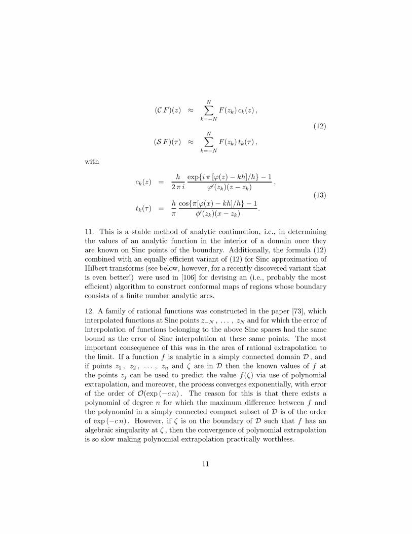
(C F )(z) ≈N∑

k=−N

F (zk) ck(z) ,

(S F )(τ) ≈N∑

k=−N

F (zk) tk(τ) ,

(12)

with

ck(z) =h

2π i

expi π [ϕ(z) − kh]/h − 1

ϕ′(zk)(z − zk),

tk(τ) =h

π

cosπ[ϕ(x) − kh]/h − 1

φ′(zk)(x− zk).

(13)

11. This is a stable method of analytic continuation, i.e., in determiningthe values of an analytic function in the interior of a domain once theyare known on Sinc points of the boundary. Additionally, the formula (12)combined with an equally efficient variant of (12) for Sinc approximation ofHilbert transforms (see below, however, for a recently discovered variant thatis even better!) were used in [106] for devising an (i.e., probably the mostefficient) algorithm to construct conformal maps of regions whose boundaryconsists of a finite number analytic arcs.

12. A family of rational functions was constructed in the paper [73], whichinterpolated functions at Sinc points z−N , . . . , zN and for which the error ofinterpolation of functions belonging to the above Sinc spaces had the samebound as the error of Sinc interpolation at these same points. The mostimportant consequence of this was in the area of rational extrapolation tothe limit. If a function f is analytic in a simply connected domain D , andif points z1 , z2 , . . . , zn and ζ are in D then the known values of f atthe points zj can be used to predict the value f(ζ) via use of polynomialextrapolation, and moreover, the process converges exponentially, with errorof the order of O(exp (−c n) . The reason for this is that there exists apolynomial of degree n for which the maximum difference between f andthe polynomial in a simply connected compact subset of D is of the orderof exp (−c n) . However, if ζ is on the boundary of D such that f has analgebraic singularity at ζ , then the convergence of polynomial extrapolationis so slow making polynomial extrapolation practically worthless.

11

On the other hand, if the above points zj belong to a domain D whichis mapped by ϕ onto the above defined strip Dd, if f ∈ Mα,d(ϕ) , and if ζeither belongs to D or is an end-point of Γ = ϕ−1(lR) , then there is a rationalfunction of the type derived in [73] which interpolates f at 2N +1 points ofΓ and for which the maximum difference between f and the rational at the

points zj and at ζ is of the order of exp(

−c n1/2)

, i.e., we can be sure that

rational extrapolation works to predict the value of f(ζ) , even though thisvalue might be difficult or impossible to compute directly. That is whereasthe success of rational extrapolation was previously based on a “gut feeling’,we now conditions under which it is guaranteed to work. Some examples ofthis type are given in [87]; other practically important ones, including notyet tried possibilities are given below.

13. A recent discovery of Stenger is the formula for indefinite convolutions[89], which has led to many novel important formulas in applications, forapproximating convolution integrals, for inverting Laplace transforms, forsolving integral equations, such as Wiener–Hopf equations, which were hith-erto considered to be difficult, for evaluating Hilbert transforms, for solvingPDE (partial differential equations) and for solving multidimensional inte-gral equations. The basic models are the integrals

p(x) =

∫ x

af(x− t) g(t) dt ,

q(x) =

∫ b

xf(t− x) g(t) dt ,

(14)

with x ∈ (a, b) (i.e., this process has not yet been studied for a more generalcontour Γ .) The “Laplace transform”

F(s) =

∫

Ef(t) e−t/s dt (15)

is required, with E any subinterval of lR = (−∞,∞) such that E ⊇ (0, b−a),exists for all s ∈ Ω+ ≡ s ∈ lC : ℜs > 0. It is shown in [89] that

p = F(J +) g and q = F(J −) g , (16)

with J + and J− defined as in (11) above.

Using the approximations of (11), i.e., J± g ≈ J ±m g with J ±

m = wA± V ,and with V defined as in (9) above, one can surmise that if J ± ≈ J±

m , thenF(J ±) ≈ F(J ±

m ) , and indeed, this was shown to be the case in [89]. Onethus gets the approximations

12

V p ≈ F (A+)V g and V q ≈ F (A−)V g (17)

with the error these approximations of the same order as the error in (6)above.Here, the matrices F (A±) can be evaluated by diagonalization of A±, (aprocedure which has always been possible numerically, to date) for exam-ple, if A+ = X S X−1 , with S = diag (s−N , . . . , sN ) , then F (A+) =X F (S)X−1 .

14. Summarizing to this point, we see that Sinc methods offer a self con-tained family of approximations of the most significant operations of calcu-lus, and with the error being of the order of that in (6) above:

Interpolation: F ∈ Mα,d(ϕ) =⇒

V F = V F (F (x) ≈ w(x)V F ) ;

Differentiation: ϕ′ F ∈ Lα,d(ϕ) =⇒

V F ′ ≈ (A+)−1 V F (or V F ′ ≈ −(A−)−1 V F ;

Indefinite Integration: F/ϕ′ ∈ Lα,d(ϕ) =⇒

V J± F ≈ A±V F ;

Quadrature: F/ϕ′ ∈ Lα,d(ϕ) =⇒∫

ΓF (x) dx ≈ h (V f)T V (1/ϕ′) ;

Indefinite Convolution: (See above for the definitions of p and q.) Morecomplicated precise conditions hold for the following, but usually it sufficesif p and q belong to Mα,d(ϕ) .

V p ≈ F (A+)V g , V q ≈ F (A−)V g ;

Hilbert Transform: See (6) & (12) above. Uniform error bounds for thefollowing hold if f ∈ Lα,d(ϕ) :

V S F ≈(

log(A−)− log(A+))

F ;

13

This result was derived recently, in [10] .

Cauchy Transforms. See (6) & (12) above. Uniform error bounds for thefollowing hold if f ∈ Lα,d(ϕ) .

(C F )(z) ≈N∑

k=−N

F (zk) ck(z) , z 6∈ Γ;

Laplace Transform Inversion: If g(s) =∫∞0 f(t) dt , then (over an interval

Γ , with ϕ : Γ → lR), and if 1 is a column vector of order m with a “1” ineach entry, then

V f ≈(

A+)−1g(

(

A+)−1)

1 ;

Uniformly accurate error bounds hold for this approximation if f ∈ Mα,d(ϕ) .

Inner Product Evaluations in Galerkin Methods. If f/ϕ′ ∈ Lα,d(ϕ) , and ifωj denotes the jth basis function, then

∫

Γf(x)ωj(x) dx ≈ h f(zj)

ϕ′(zj).

15. The above one dimensional convolution procedure extends readily tomultidimensional convolutions. And while the approximation of one di-mensional convolutions requires the diagonalization of a matrix and thusseemingly requires more work than we are normally used to expend on anumerical method, this amount of work is relatively small for solution ofpartial differential equations.

16. The solution of PDE that are expressed via integrals of Green’s func-tions is a straight forward application of Sinc convolution, but to achievethis, one requires the multidimensional “Laplace transform” of the Green’sfunction. Stenger was lucky in this endeavor, in that he was able to obtainexplicit expressions of all of the free space multidimensional Green’s func-tions known to him for Poisson, biharmonic, wave, and heat problems. Thederivations of these are given in [121 ]. Also in [121], Stenger gives explicitalgorithms for the evaluation of the Green’s function convolution integrals,first over rectangular, and then also over curvilinear regions. It has thusbecome possible to achieve a highly efficient and accurate approximation ofmultidimensional Green’s function convolution integrals via the use of a very

14

small number of multiplications of one dimensional matrices i.e., via separa-tion of variables . We are thus able to circumvent the use of large matricesrequired via use of classical finite difference or finite element methods, andthus, to get uniformly accurate solution via use of considerably less effort.

For example, to evaluate the solution of a Poisson problem for a functionU , over a planar region B, with

U(x, y) =

∫ ∫

BG(x− ξ, y − η) e(ξ, η) dξ dη .

G(x, y) = 1

2πlog

1√

x2 + y2,

(18)

and with e a forcing function that might be unbounded on the boundary of Bbut is integrable over B , we need the two dimensional “Laplace transform”G of the Green’s function G , i.e.,

G(u, v) =

∫ ∞

0

∫ ∞

0exp

(

−xu− y

v

)

G(x, y) dx dy

=

(

1

u2+

1

v2

)−1

·

·(

−1

4+

1

2π

(

v

u(γ − ln(v)) +

u

v(γ − ln(u))

))

.

(19)

Thus, if B is a rectangular region such as B = (0, 1) × (0, 1), if A± arethe Sinc indefinite integration matrices of order m = 2N + 1 over (0, 1),with A+ = X SX−1 , A− = Y S Y −1 , with S a diagonal matrix, S =diag(s−N , . . . , sN ) , withXi = X−1 and Y i = Y −1, with G the matrix with(i, j)th entry G(si , sj) , and with E the matrix with (i, j)th entry e(zi, zj),and where the zk denote Sinc points, we can approximate U(zi, zj) ≈ Uij

via use of the following Matlab program:

U = X ∗ (G. ∗ (Xi ∗ E ∗Xi.′)) ∗X.′;U = U + Y ∗ (G. ∗ (Y i ∗ E ∗Xi.′)) ∗X.′;U = U +X ∗ (G. ∗ (Xi ∗ E ∗ Y i.′)) ∗ Y.′;U = U + Y ∗ (G. ∗ (Y i ∗ E ∗ Y i.′)) ∗ Y.′;

This approximate solution has a uniform error of the order of that on theright hand side of (6), provided that each of the functions, e(·, y) for each

15

fixed y ∈ (0, 1) and e(x, ·) for each fixed x ∈ (0, 1) are analytic, and providedthat U is uniformly bounded on B .

We may note that this procedure just involves the product of a few one di-mensional matrices (separation of variables!). Similarly, higher dimensionalproblems, including, e.g., problems over a rectangular region B in lR3, orover B × (0, T ) are not much more difficult to solve.

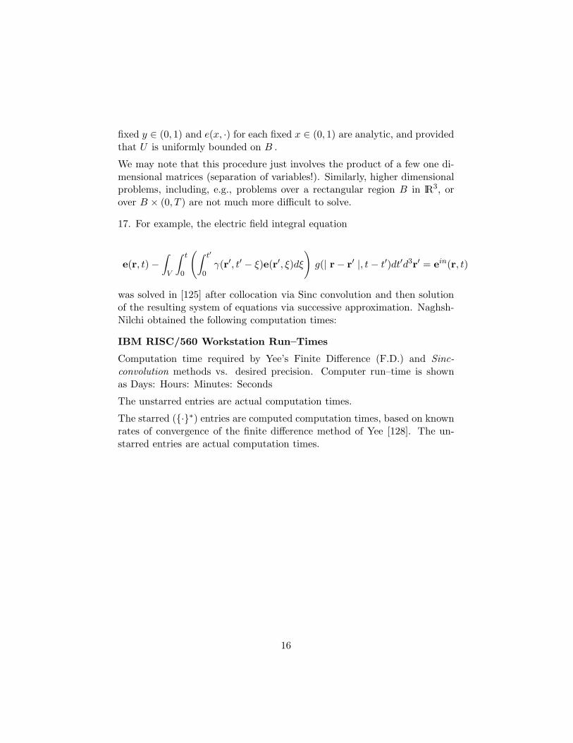
17. For example, the electric field integral equation

e(r, t)−∫

V

∫ t

0

(

∫ t′

0γ(r′, t′ − ξ)e(r′, ξ)dξ

)

g(| r− r′ |, t− t′)dt′d3r′ = ein(r, t)

was solved in [125] after collocation via Sinc convolution and then solutionof the resulting system of equations via successive approximation. Naghsh-Nilchi obtained the following computation times:

IBM RISC/560 Workstation Run–Times

Computation time required by Yee’s Finite Difference (F.D.) and Sinc-convolution methods vs. desired precision. Computer run–time is shownas Days: Hours: Minutes: Seconds

The unstarred entries are actual computation times.

The starred (·∗) entries are computed computation times, based on knownrates of convergence of the finite difference method of Yee [128]. The un-starred entries are actual computation times.

16

Acc. F. D. Run-Time Sinc–Conv. Run-Time

10−1 ≈ 1 second ≈ 1 second

10−2 000:00:00:27 000:00:00:06

10−3 003:00:41:40∗ 000:00:02:26

10−4 > 82 years∗ 000:00:43:12

10−5 > 800,000 years∗ 000:06:42:20

10−6 > 8.2 billion years∗ 001:17:31:11

18. Many other PDE have been solved since via the Sinc convolution ap-proach, each illustrating the ease of use and accuracy of Sinc methods. Thetutorial [121] contains examples of the solution of PDE over curvilinearregions, solution of nonlinear PDE, one of which (the nonlinear integro–differential equation in [10, §4.3.1]) no-one else was able to solve via anyother method, and the ease of solution of wave and time problems via use ofNeumann type iteration, which works, in essence for Sinc methods wheneverit works in theory.

19. In [17] Morse & Feshbach discuss the possibility of use of separationof variables to solve three dimensional Laplace and Helmholtz equations.They conclude via use of the Stackel determinant, that there are essentiallyonly 13 coordinate systems for which this is possible. The key to success ofthis procedure is, in essence is to be able to transform the problem over theoriginal region into a similar one over a rectangular region. They would thenbe able to use one-dimensional methods to solve multidimensional problems.Stenger shows in [10] that such separation of variables is possible for Poisson,wave and heat problems in all dimensions. One reason for this is that theSinc methods of this package enable solutions of PDE without approximationof the highest derivatives. The procedure is based on the above convolutionmethod. One does, however, require one additional property for success,which is that the coefficients of PDE as well as the patches of the boundaryof the region are analytic in each variable, with all other variables held fixed,

17

and real. PDE from applications that are modeled via use of calculus do,in fact have this feature, under the assumption that such PDE are modeledby scientists and engineers, via use of calculus. In such circumstances, Sincmethods also yield exponential convergence, and combined with the separa-tion of variables referred to above, we are able to obtain significant increasesin the rates of convergence over classical methods.

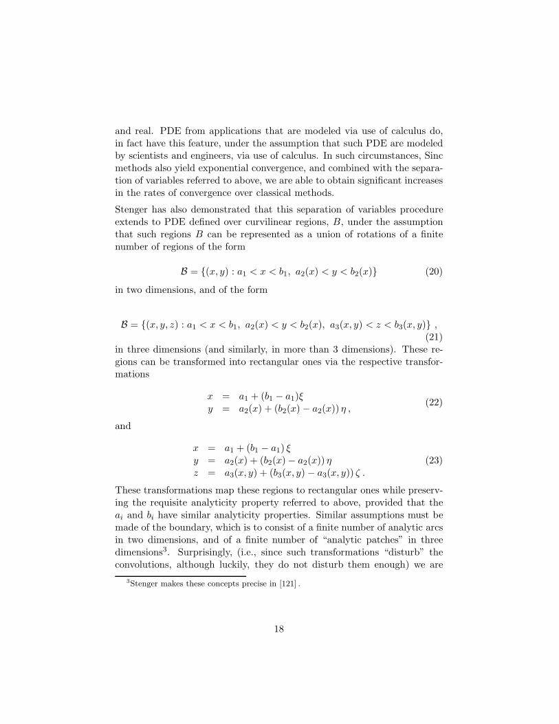
Stenger has also demonstrated that this separation of variables procedureextends to PDE defined over curvilinear regions, B, under the assumptionthat such regions B can be represented as a union of rotations of a finitenumber of regions of the form

B = (x, y) : a1 < x < b1, a2(x) < y < b2(x) (20)

in two dimensions, and of the form

B = (x, y, z) : a1 < x < b1, a2(x) < y < b2(x), a3(x, y) < z < b3(x, y) ,(21)

in three dimensions (and similarly, in more than 3 dimensions). These re-gions can be transformed into rectangular ones via the respective transfor-mations

x = a1 + (b1 − a1)ξy = a2(x) + (b2(x)− a2(x)) η ,

(22)

and

x = a1 + (b1 − a1) ξy = a2(x) + (b2(x)− a2(x)) ηz = a3(x, y) + (b3(x, y)− a3(x, y)) ζ .

(23)

These transformations map these regions to rectangular ones while preserv-ing the requisite analyticity property referred to above, provided that theai and bi have similar analyticity properties. Similar assumptions must bemade of the boundary, which is to consist of a finite number of analytic arcsin two dimensions, and of a finite number of “analytic patches” in threedimensions3. Surprisingly, (i.e., since such transformations “disturb” theconvolutions, although luckily, they do not disturb them enough) we are

3Stenger makes these concepts precise in [121] .

18

still able to use separation of variables to evaluate the convolution inte-grals after such transformations are made, via use of the original “Laplacetransformed” Green’s functions.

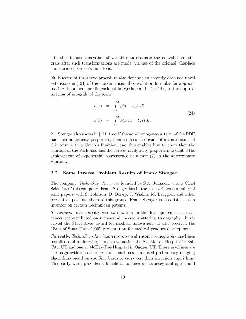
20. Success of the above procedure also depends on recently obtained novelextensions in [121] of the one dimensional convolution formulas for approxi-mating the above one dimensional integrals p and q in (14) , to the approx-imation of integrals of the form

r(x) =

∫ x

ag(x− t, t) dt ,

s(x) =

∫ x

ak(x , x− t , t) dt .

(24)

21. Stenger also shows in [121] that if the non-homogeneous term of the PDEhas such analyticity properties, then so does the result of a convolution ofthis term with a Green’s function, and this enables him to show that thesolution of the PDE also has the correct analyticity properties to enable theachievement of exponential convergence at a rate (7) in the approximatesolution.

2.2 Some Inverse Problem Results of Frank Stenger.

The company, TechniScan Inc., was founded by S.A. Johnson, who is ChiefScientist of this company. Frank Stenger has in the past written a number ofjoint papers with S. Johnson, D. Borup, J. Wiskin, M. Berggren and otherpresent or past members of this group. Frank Stenger is also listed as aninventor on certain TechniScan patents.

TechniScan, Inc. recently won two awards for the development of a breastcancer scanner based on ultrasound inverse scattering tomography. It re-ceived the Stoel-Rives award for medical innovation. It also received the”Best of State Utah 2005” presentation for medical product development.

Currently, TechniScan Inc. has a prototype ultrasonic tomography machinesinstalled and undergoing clinical evaluation the St. Mark’s Hospital in SaltCity, UT and one at McKay-Dee Hospital in Ogden, UT. These machines arethe outgrowth of earlier research machines that used preliminary imagingalgorithms based on use Sinc bases to carry out their inversion algorithms.This early work provides a beneficial balance of accuracy and speed and

19

efficient use of computer memory since only 4 samples per wavelength arerequired using Sinc bases, whereas at least 8 samples per wavelength arerequired via other bases or sampling schemes.

Sinc basis sampling was featured in a TechniScan, Inc. publication outlininga method, using inverse scattering, that increased speed and accuracy forremote SONAR imaging of buried objects on the ocean bottom [129]

Other articles featuring Sinc methods of inverse problems and imaging in-clude [130 , 131 , 132] .

We list here some inverse problems results of Frank Stenger which haveyet been used commercially. The results listed here are based on the 3–dHelmholtz equation,

∇2 u(r) + k2(1 + f(r))u(r) = 0 in B , (25)

where B is a bounded region in lR3 , f(r) = c20/c2(r)−1, with c(r) and c0 the

speeds of sound in B and in lR \ B respectively, so that f = 0 on lR3 B, andwith k = ω/c0 . A source with respect to the equation (25) is any functionv which satisfies in B the equation

∇2 v(r) + k2 v(r) = 0 . (26)

It may be shown that the solution u of (25) resulting from a source v satis-fying (26) satisfies the integral equation

u(r)− v(r) = k2∫ ∫ ∫

BG(r , r′ , k) f(r′)u(r′) dr′ , (27)

where

G(r , r′ , k) =exp (i k |r − r′|)

4π |r − r′| . (28)

For example, two easily produced sources in applications are a plane waveand a spherical source. These are given respectively by

v(r) = exp(i k · r) , |k| = kv(r) = G(r , rs , k) , rs 6∈ B . (29)

We also denote two points on the exterior of B : rs – a source point, and rd– a detector point.

20

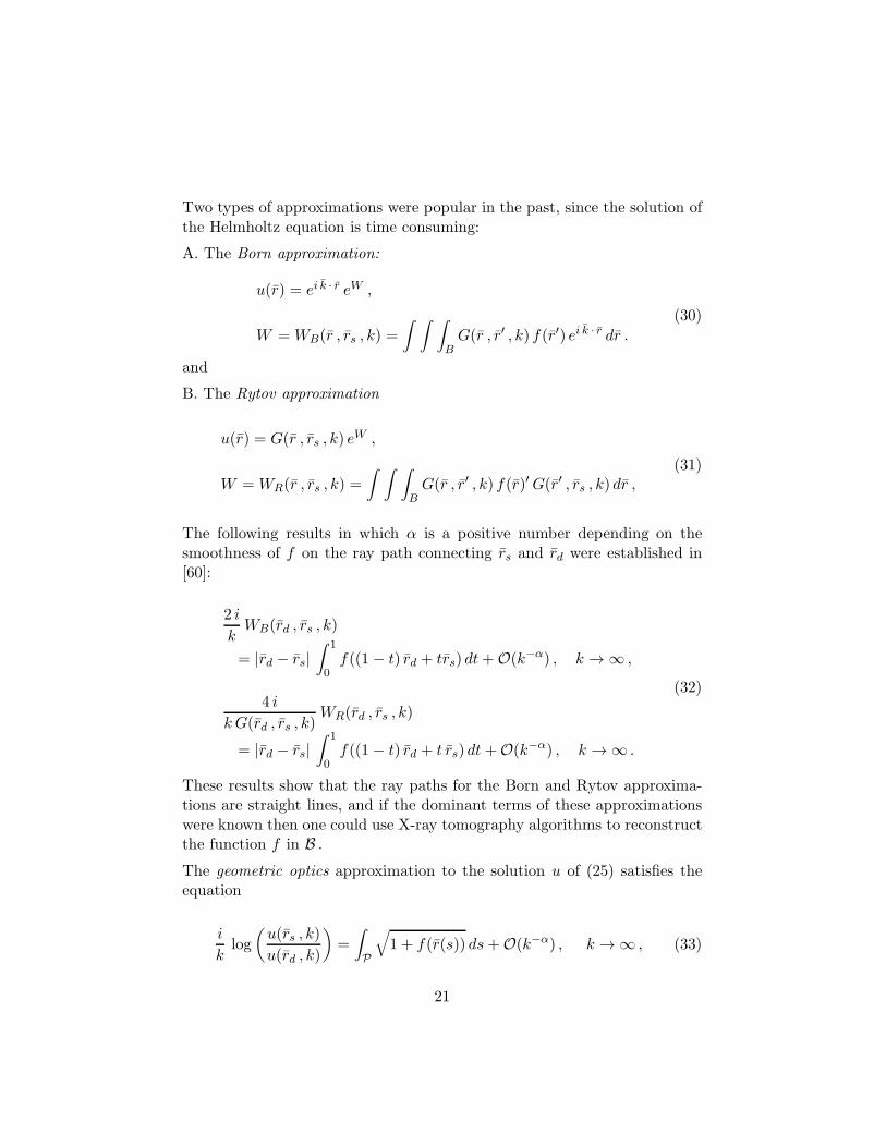
Two types of approximations were popular in the past, since the solution ofthe Helmholtz equation is time consuming:

A. The Born approximation:

u(r) = ei k · r eW ,

W =WB(r , rs , k) =

∫ ∫ ∫

BG(r , r′ , k) f(r′) ei k · r dr .

(30)

and

B. The Rytov approximation

u(r) = G(r , rs , k) eW ,

W =WR(r , rs , k) =

∫ ∫ ∫

BG(r , r′ , k) f(r)′G(r′ , rs , k) dr ,

(31)

The following results in which α is a positive number depending on thesmoothness of f on the ray path connecting rs and rd were established in[60]:

2 i

kWB(rd , rs , k)

= |rd − rs|∫ 1

0f((1− t) rd + trs) dt+O(k−α) , k → ∞ ,

4 i

k G(rd , rs , k)WR(rd , rs , k)

= |rd − rs|∫ 1

0f((1− t) rd + t rs) dt+O(k−α) , k → ∞ .

(32)

These results show that the ray paths for the Born and Rytov approxima-tions are straight lines, and if the dominant terms of these approximationswere known then one could use X-ray tomography algorithms to reconstructthe function f in B .

The geometric optics approximation to the solution u of (25) satisfies theequation

i

klog

(

u(rs , k)

u(rd , k)

)

=

∫

P

√

1 + f(r(s)) ds+O(k−α) , k → ∞ , (33)

21

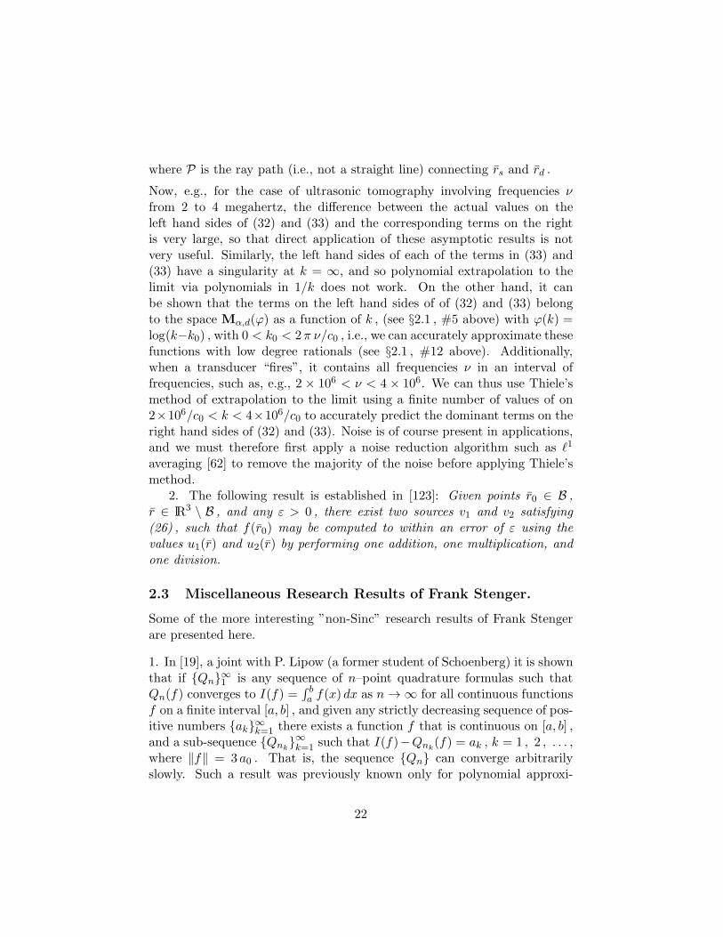
where P is the ray path (i.e., not a straight line) connecting rs and rd .

Now, e.g., for the case of ultrasonic tomography involving frequencies νfrom 2 to 4 megahertz, the difference between the actual values on theleft hand sides of (32) and (33) and the corresponding terms on the rightis very large, so that direct application of these asymptotic results is notvery useful. Similarly, the left hand sides of each of the terms in (33) and(33) have a singularity at k = ∞, and so polynomial extrapolation to thelimit via polynomials in 1/k does not work. On the other hand, it canbe shown that the terms on the left hand sides of of (32) and (33) belongto the space Mα,d(ϕ) as a function of k , (see §2.1 , #5 above) with ϕ(k) =log(k−k0) , with 0 < k0 < 2π ν/c0 , i.e., we can accurately approximate thesefunctions with low degree rationals (see §2.1 , #12 above). Additionally,when a transducer “fires”, it contains all frequencies ν in an interval offrequencies, such as, e.g., 2 × 106 < ν < 4 × 106. We can thus use Thiele’smethod of extrapolation to the limit using a finite number of values of on2×106/c0 < k < 4×106/c0 to accurately predict the dominant terms on theright hand sides of (32) and (33). Noise is of course present in applications,and we must therefore first apply a noise reduction algorithm such as ℓ1

averaging [62] to remove the majority of the noise before applying Thiele’smethod.

2. The following result is established in [123]: Given points r0 ∈ B ,r ∈ lR3 \ B , and any ε > 0 , there exist two sources v1 and v2 satisfying(26) , such that f(r0) may be computed to within an error of ε using thevalues u1(r) and u2(r) by performing one addition, one multiplication, andone division.

2.3 Miscellaneous Research Results of Frank Stenger.

Some of the more interesting ”non-Sinc” research results of Frank Stengerare presented here.

1. In [19], a joint with P. Lipow (a former student of Schoenberg) it is shownthat if Qn∞1 is any sequence of n–point quadrature formulas such thatQn(f) converges to I(f) =

∫ ba f(x) dx as n→ ∞ for all continuous functions

f on a finite interval [a, b] , and given any strictly decreasing sequence of pos-itive numbers ak∞k=1 there exists a function f that is continuous on [a, b] ,and a sub-sequence Qnk

∞k=1 such that I(f)−Qnk(f) = ak , k = 1 , 2 , . . . ,

where ‖f‖ = 3 a0 . That is, the sequence Qn can converge arbitrarilyslowly. Such a result was previously known only for polynomial approxi-

22

mation of continuous functions. Moreover, it extends Polya’s result on thenon-convergence of the Newton–Cotes quadrature rules for all continuousfunctions.

2. In [32] Rosenberg and Stenger obtained an interesting result involvingthe “bisection” of triangles. Given a triangle T0 with smallest interior angleα , the process of bisection of this triangle is to draw a line segment fromthe mid-point of the longest edge to the opposite vertex (if there are two orthree of the edges that are longest, then it is immaterial which longest edgeis selected), thus producing two triangles. The result proved in [32] statesthat if T is any member of the family of triangles produced by first bisectingT0 to produce T1 and T2 , then bisecting each of the two new triangles, and soon, then the size of the smallest interior angle of T is at least α/2 . Althoughit was unknown to the authors of [32] when they wrote their paper, that theangles of triangles do not go to zero upon repeated bisection was a conjectureof finite element users, the result of which was required for convergence.

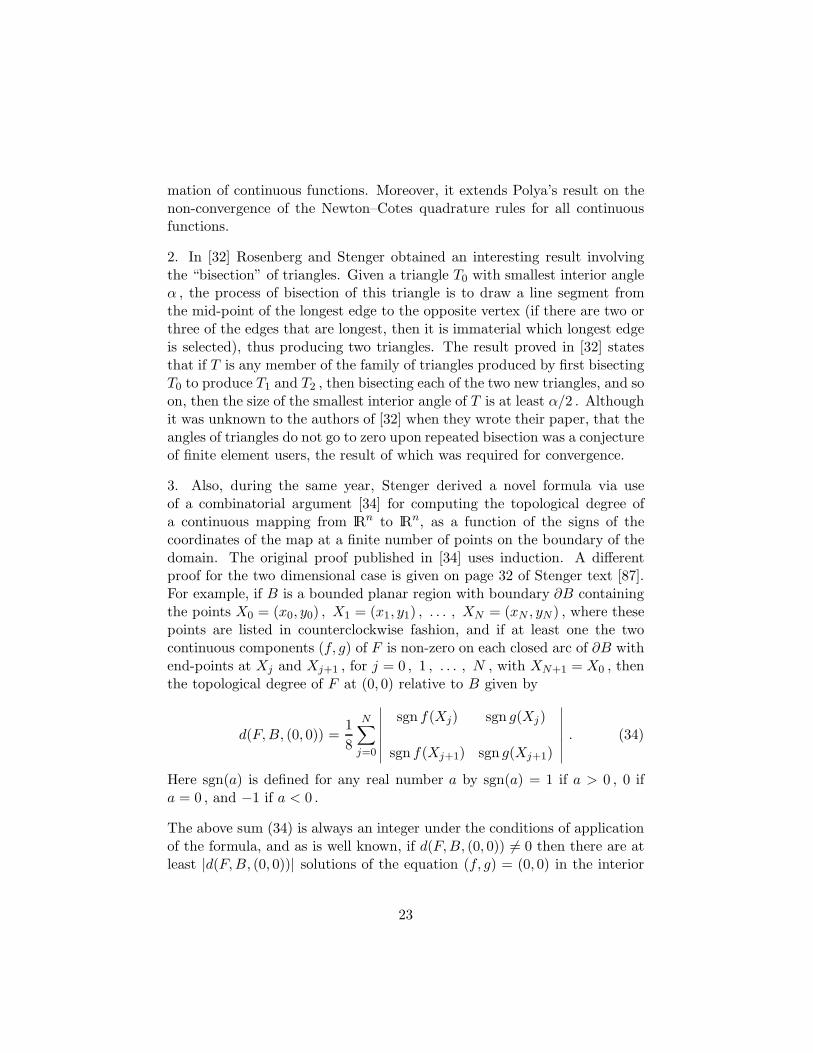
3. Also, during the same year, Stenger derived a novel formula via useof a combinatorial argument [34] for computing the topological degree ofa continuous mapping from lRn to lRn, as a function of the signs of thecoordinates of the map at a finite number of points on the boundary of thedomain. The original proof published in [34] uses induction. A differentproof for the two dimensional case is given on page 32 of Stenger text [87].For example, if B is a bounded planar region with boundary ∂B containingthe points X0 = (x0, y0) , X1 = (x1, y1) , . . . , XN = (xN , yN ) , where thesepoints are listed in counterclockwise fashion, and if at least one the twocontinuous components (f, g) of F is non-zero on each closed arc of ∂B withend-points at Xj and Xj+1 , for j = 0 , 1 , . . . , N , with XN+1 = X0 , thenthe topological degree of F at (0, 0) relative to B given by

d(F,B, (0, 0)) =1

8

N∑

j=0

∣

∣

∣

∣

∣

∣

∣

sgn f(Xj) sgn g(Xj)

sgn f(Xj+1) sgn g(Xj+1)

∣

∣

∣

∣

∣

∣

∣

. (34)

Here sgn(a) is defined for any real number a by sgn(a) = 1 if a > 0 , 0 ifa = 0 , and −1 if a < 0 .

The above sum (34) is always an integer under the conditions of applicationof the formula, and as is well known, if d(F,B, (0, 0)) 6= 0 then there are atleast |d(F,B, (0, 0))| solutions of the equation (f, g) = (0, 0) in the interior

23

of B .

4. In a recent colloquium talk in Math. at the Univ. of Utah, David Baileyfrom Lawrence Livermore Labs. stated that in computing π to 20 billionplaces, his group used Sinc quadrature to check their results.

5. Asymptotic methods are, of course important, especially for derivingthe dominant term of an expansion. It is also frequently possible to set upan indefinite integral, or a Volterra integral equation for either boundingthe error of a truncated expansion, or for obtaining more terms of of anexpansion. This integral, or Volterra integral equation can now be evaluatedto uniform accuracy on the whole interval of interest via Sinc methods. Forexample, a derived asymptotic result (of an integral, a differential equation,etc.) might take the form

f(x) = g(x) (1 + ε(x)) , x ∈ (a ,∞) ,

with g(x) explicitly known, followed by an estimate such as, ε(x) = O (x−c) ,or a bound on ε(x) which might depend on x ∈ (a ,∞) . Sinc methods enablea simple expression for ε(x) that can be evaluated to arbitrary accuracy forany x ∈ (a ,∞) . See the IVP examples section of Sinc-Pack.

6. In [8] Stenger proved, among other things, if Qn(f) is the n–point Gaus-sian quadrature approximation to I(f) =

∫ 1−1 f(x) dx , if f is analytic on the

unit disc and integrable over (−1, 1) , and if the even derivatives f (2k)(0) off are all of one sign, then Qn(f) converges monotonically to I(f) .

2.4 Program Packages of Frank Stenger.

The following program packages exist:

i. The quadrature package, ALGORITHM 614. A FORTRAN Subroutinefor Numerical Integration in Hp, written jointly with K. Sikorski andJ. Schwing, in ACM TOMS 10 (1984) 152–160.

This routine, originally written in FORTRAN, evaluates integrals intwo ways: (a) To an arbitrary given accuracy of ε ; or (b) Using a mini-mal number of points to achieve and accuracy, when f/vp′ ∈ Mα,d(ϕ) ,and we know both α and d . It is time to improve it, by rewriting itin Matlab, and by making it dependent on ϕ , thus shortening theprogram considerably.

24

ii. The ODE–IVP package [106], ODE – IVP – PACK via Sinc Indefi-nite Integration and Newton’s Method, with SA. Gustafson, B. Keyes,M. O’Reilly, and K. Parker, published in “Numerical Algorithms” 20(1999) 241–268 .

This package can be downloaded from Netlib. It is similar to BillGear’s package for solving initial value problems of ordinary differentialequations, except that it differs from his, or other packages, in thefollowing ways:

• a. It uses Sinc indefinite integration, rather than step–by–stepmethods based on finite differences;

• b. The package yields arbitrary, uniform accuracy, for all prob-lems, whereas other packages are accurate to within a least squareserror;

• c. Other packages work only for finite intervals, whereas thepresent one yields solutions over arbitrary intervals, finite or in-finite, and even contours;

• d. Classical methods suffer due to problems of instability, whereasthis package does not; and

• e. Classical methods have trouble dealing with Stiff problems,whereas this package does not.

iii. The PDE package, Ptolemy, [107], prepared for his Ph.D. work, by K.Parker, in 1999.

It is written in Maple. It converts an elliptic PDE and IE (integralequations) over a curvilinear region to a system of algebraic equations,based on Sinc approximation of the derivatives of the PDE.

iv. Handbook of Sinc Numerical Methods, published by CRC Press (2010).

It consists of two parts:

(a) A Tutorial of Sinc Methods, a 470–page text, i containing novelderivations of the Sinc theory and one dimensional Sinc methods, viaminimization of the use of complex variables, then derives novel meth-ods of solution of PDE and integral equations via use of Sinc convo-lution and boundary integral methods. It is moreover shown in thetutorial that all solutions of linear PDE can be obtained via use of one

25

dimensional Sinc methods, (i.e., via separation of variables– Stengerexpends considerable effort to show that this is always possible) evenover curvilinear regions, yielding solutions that are uniformly accurateand converge exponentially, as a function of the size of the one dimen-sional matrices. The multidimensional Laplace transforms of Green’sfunctions are required for success of this endeavor, and to this end,Stenger was able to obtain the Laplace transforms of all of the freespace Green’s functions known to him. The resulting solution tech-niques are often orders of magnitude faster than current methods inuse.

(b) A set of approximately 450 Matlab programs, written by Stenger.The use of some of these programs is illustrated in the above citedtutorial, for solving a variety of one dimensional and PDE problems.These are contained in a CD published with the text ”Handbook ofSinc Numerical Methods”, CRC Press (2010).

2.5 Textbooks.

The following textbooks are authored or co-authored by Stenger:

a. Numerical Methods Based on Sinc and Analytic Functions, approxi-mately 565 pages, Computational Math. Series, Vol. 20, Springer–Verlag (1993).

b. Selected Topics of Approximation and Computation, with K. Sikorskiand M. Kowalski, approximately 349 pages, Oxford University Press(1995). Was awarded “First Prize” by the Minister of Education inPoland, for the best research in 1995.

c. Numerical Analysis, textbook, with J. McNamee, 531 pages, in manuscript.McNamee has been deceased for over 12 years. The book was startedby him and me about 20 years ago. During the past year I wrotethree additional chapters, 2 on Sinc methods and one on asymptoticmethods.

d. Handbook of Sinc Numerical Methods, CRC Press (2010). About 490pages. Completed in 2010. this was already discussed above.

The following text is a nice introduction to Sinc methods:

26

e. Sinc Methods for Quadrature and Differential Equations, by J. Lund &K. Bowers, approximately 334 pages, SIAM (1992).

Bibliography.

[1] Error Bounds for Asymptotic Solution of Second Order DifferentialEquations Having an Irregular Singularity of Arbitrary Rank, (withF.W.J. Olver), SIAM J. Numer. Anal. 12 (1965) 244–249.

[2] Some Remarks on Asymptotics, Notes, Canadian Math. Congress(1965).

[3] Error Bounds for Asymptotic Solution of Differential Equations: I. TheDistinct Eigenvalue Case, J. Res. NBS – B. Math. and Math. Phys.708 (1966) 167–186.

[4] Bounds on the Error of Gauss–type Quadratures, Num. Math. 8 (1966)150–160.

[5] Error Bounds for the Evaluation of Integrals by Repeated Gauss–typeFormulas, Num. Math. 9 (1966) 200–213.

[6] Error Bounds for Asymptotic Solutions of Differential Equations, II.The General Case, J. Res. NBS – B. Math. and Math. Phys. 708(1966) 187–210.

[7] Construction of Fully Symmetric Numerical Integration Formulas, (withJ. McNamee), Num. Math. 10 (1967) 327–344.

[8] Kronecker Product Extension of Linear Operators, SIAM J. Numer.Anal. 5 (1968) 422–435.

[9] The Asymptotic Approximation of Certain Integrals, SIAM J. Math.Anal. 1 (1970) 392–404.

[10] Movable Singularities and Quadrature, (with R.F. Goodrich), Math.Comp., 24 (1970) 283–300.

[11] On the Asymptotic Solution of Two First Order Differential Equationswith Large Parameter, Funkt. Ekvac. 13 (1970) 1–18.

[12] Movable Singularities and Quadrature, (with R.F. Goodrich), Math.Comp., 24 (1970) 283–300.

27

[13] The Lowdin–type Projection Operators for SU(1,1), (with J. Patera),in manuscript (1970).

[14] Tabulation of Certain Fully Symmetric Numerical Integration Formu-las of Degree 3, 5, 7, 9, and 11, Math. Comp. 25 (1971) 935.

[15] Seven, Nine, and Eleven–Degree Fully Symmetric Numerical Integra-tion Formulas, in “Approximate Calculation of Multiple Integrals”, byA.H. Stroud, Prentice Hall (1971).

[16] Whittaker’s Cardinal Function in Retrospect, (with J. McNamee andE.L. Whitney), Math. Comp. 25 (1971) 141–154.

[17] Constructive Proofs for Approximation by Inner Functions, J. Approx.Theory 4 (1971) 372–386.

[18] The Reduction of Two Dimensional Integrals into a Finite Number ofOne Dimensional Integrals, Aeq. Math. 6 (1971) 278–287.

[19] How Slowly Can Quadrature Formulas Converge? (with P. Lipow),Math. Comp. 26 (1972) 917–922.

[20] Transform Methods of Obtaining Asymptotic Expansions of DefiniteIntegrals, SIAM J. Math. Anal. 3 (1972) 20–30.

[21] Asymptotic Solution of First Order Ordinary Differential Equationswith Large Parameter, (with J. Oberholzer) in manuscript (1972).

[22] How Slowly Can Quadrature Formulas Converge? (with P. Lipow),Math. Comp. 26 (1972) 917–922.

[23] The Approximate Solution of Wiener–Hopf Integral Equations, J.Math. Anal. Appl. 37 (1972) 687–724.

[24] The Approximate Solution of Convolution–type Integral Equations,SIAM J. Math. Anal. 4 (1973) 536–555.

[25] An Algorithm for Solving Wiener–Hopf Integral Equations, COMMACM 16 (1973) 708–710.

[26] Integration Formulas Based on the Trapezoidal Formula, J. Inst. MathsApplics, 12 (1973) 103–114.

28

[27] On the Convergence and Error of the Bubnov–Galerkin Method, “SIAMProceedings of the Conference on the Numerical Solution of OrdinaryDifferential Equations”, Springer–Verlag Lecture Notes in Mathemat-ics 362 (1973) 448–464.

[28] An Extremal Problem for Polynomials with a Prescribed Zero, (withQ.I. Rahman) Proc. AMS 43 (1974) 84–90.

[29] A Comparison of Some Deterministic and Monte Carlo QuadratureSchemes, (22 typed pages), in manuscript (1974).

[30] An Approximate Convolution Equation of a Given Response, (withW.B. Gearhart, in “Optimal Control Theory and Its Applications”Springer–Verlag Lecture Notes on Economics and Mathematical Sys-tems 106 (1974) 168–196.

[31]Minimum–point Quadrature Formulas with Positive Weights, (24 typedpages) (1974).

[32] A Lower Bound on the Angles of Triangles Constructed from a GivenTriangle, (with I. Rosenberg) Math. Comp. 29 (1975) 390–395.

[33] On the Approximate Solution of the nonlinear equation u′′ = u − u3,(with J. Chauvette) J. Math. Anal. Appl. 5 (1975) 229–243.

[34] An Algorithm for the Topological Degree of a Mapping in lRn, Bull.AMS 81 (1975) 179–182.

[35] Computing the Topological Degree of a Mapping in Rn, Num. Math.25 (1975) 23–38.

[36] An Integral with Respect to a Measure is an Integral over a Region, inmanuscript (1975).

[37] On the Asymptotic Solution of the Riccati Differential Equation, (21typed pages) Presented to Canada Math. Congress Conference, June,1975, in manuscript.

[38] An Analytic Function which is an Approximate Characteristic Func-tion, SIAM J. Numer. Anal. 12 (1975) 239–254.

[39] Connection Between a Cauchy System Representation of Kalaba andFourier Transforms, App. Math. and Comput. 1 (1975) 83–91.

29

[40] An Integral with Respect to a Measure is an Integral over a Region, inmanuscript (1975).

[41] A Two Dimensional Method of Bisections for Solving Nonlinear Equa-tions, (with C. Harvey) Quart. Applied Math. 33 (1976) 351–368.

[42] Numerical Solution of Hilbert’s Problem, (with T.Y. Li and Y. Ikebe)in “Theory of Approximation with Applications”, Acad. Press, Inc.(1976) eds. A.G. Law and B. Sahney, 338–358.

[43] Approximations via the Whittaker Cardinal Function, J. Approx. The-ory 17 (1976) 222–240.

[44] Distinct Sums over Subsets, (with F. Hanson and J.M. Steele) Proc.AMS 66 (1977) 179–180.

[45] Remarks on Integration Formulas Based on the Trapezoidal Formula,J. Inst. Maths Applics, 19 (1977) 145–147.

[46] Optimum Convergence of Minimum Norm Approximations in Hp, Nu-mer. Math. 29 (1978) 345–362).

[47] Upper and Lower Estimates on the Rate of Convergence of Approxi-mations in Hp, Bull. AMS 84 (1978) 145–148.

[48] Accuracy of Methods in Geophysics Modeling, in Proceedings of“Workshop on Modeling of Electrical and Electromagnetic Methods”,Lawrence Berkeley Lab. (1978) 147–157.

[49] Cardinal–type Approximation of a Function and Its Derivatives, (withL. Lundin), SIAM J. Numer. Anal. 10 (1979) 139–160.

[50] A Sinc Galerkin Method of Solution of Boundary Value Problems,Math. Comp. 33 (1979) 85–109.

[51] Ultrasonic Transmission Tomography Based on the Inversion of theHelmholtz Wave Equation for Plane and Spherical Wave Insonifica-tion, (with S. Johnson) (Canadian) Applied Math. Notes 4 (1979)102–127.

[52] Perturbation Methods for Reconstructing 3–D Complex Acoustic Ve-locity and Impedance in Circular Geometries with Spherical Waves,(with J.S. Ball, and S.A. Johnson) “Ninth International Symposium

30

on Acoustical Imaging, Acoustical Imaging”, 9 (1979) Plenum Press,New York.

[53] An Algorithm for Computing the Electromagnetic Scattered Field froman Axially Symmetric Body with an Impedance Boundary Condition,(with M. Hagmann and J. Schwing) J. Math. Anal. Appl. 78 (1980)531–573.

[54] Electromagnetic Scattering due to an Axially–Symmetric Body withCorners and Edges, in manuscript (1980).

[55] Unique Advantages of Sinc Function Basis in the Method of Moments,(with M. Hagmann) in “Proceedings of the Conference on Electromag-netic Insonification,” IEEE 54 (1980) 35–37.

[56] Explicit Inversion of the Helmholtz Equation for Ultrasound Insonifica-tion and Spherical Detection, (with J. Ball and S.A. Johnson) Acous-tical Imaging (ed.: K.Y. Wang) 9 (1980) 451–461.

[57] An Algorithm for Ultrasonic Tomography Based on the Inversion of theHelmholtz Equation, “Proceedings of the Conference on the Numeri-cal Solution of Nonlinear Equations, Eigenvalue Problems,” Springer–Verlag Lecture Notes in Mathematics 878 (1980) 371–406.

[58] Numerical Methods Based on the Whittaker Cardinal, or Sinc Func-tions, SIAM Rev. 23 (1981) 165–224.

[59] A Three Dimensional Reflection and Diffraction Tomography Scan-ner, with S.A. Johnson, M.J. Berggren, C.H. Wilcox and E. Jensen,“Ultrasonic Imaging” 3 (1981) 200.

[60] Asymptotic Ultrasonic Inversion Based on Using More than One Fre-quency, Acoustical Imaging 11 (1982) 425–444.

[61] Wave Equations and Inverse Solutions for Soft Tissue, (with J. Ball,M. Berggren, S.A. Johnson, C. Wilcox), Acoustical Imaging 11 (1982)409–424.

[62] An Adaptive, Noise Tolerant, Frequency Extrapolation Algorithm forDiffraction Connected Ultrasonic Tomography, (with M.J. Berggren,S.A. Johnson and Y. Li), IEEE Ultrasonics Symposium Proceedings(1983) 726–731.

31

[63] Polynomial, Sinc, and Rational Function Methods for ApproximatingAnalytic Functions, pp. 244–251 of Proceedings of the 1983 TampaConference on Rational Approximation and Interpolation, Springer–Verlag Lecture Notes in Math., #1105.

[64] Optimal Quadratures in Hp Spaces, with K. Sikorski, ACM TOMS 10(1984) 140–151.

[65] Sinc Methods of Approximate Solution of Partial Differential Equa-tions, IMACS Proceedings on Advances in Computer Methods forPartial Differential Equations, Philadelphia, P.A., 1984, pp. 244–251.

[66] Sinc Methods for Solving Partial Differential Equations, in “Contribu-tions of Mathematical Analysis to the Approximate Solution of PartialDifferential Equations”, A. Miller, Ed., Proceedings of the Centre forMathematical Analysis, Australian National University, V. 7, 1984,pp. 40–64.

[67] Sinc Approximation for Cauchy–Type Singular Integrals over Arcs,with D. Elliott, Aus. Math. Soc. V. 42 (2000) 87–97.

[68] A Method of Bisections for Solving a System of Nonlinear Equations,(with A. Eiger and K. Sikorski) ACM TOMS(1984).

[69] Rational Function Frequency Extrapolation in Ultrasonic Tomography,(with M.J. Berggren, S. Johnson and C. Wilcox) in “Wave Phenomena,Modern Theory and Applications”, C. Rogers and T.B. Moodie, eds.North–Holland (1984) 19–34.

[70] Fast Iterative Algorithms for Inverse Scattering Solutions of theHelmholtz and Riccati Wave Equations, (with S.A. Johnson, Y. Zhou,M.K. Tracy and M.J. Berggren) Acoustical Imaging, 13 (1984) 75–87.Inverse Scattering Solutions by Sinc Basis, Multiple Source MomentMethod, –Part III: Fast Algorithms, with S.A. Johnson, Y. Zhou, M.L.Tracy, and M.J. Berggren, “Ultrasonic Imaging”, 6 (1984) 103–116.

[71] ALGORITHM 614. A FORTRAN Subroutine for Numerical Integra-tion in Hp, with J. Schwing and K. Sikorski, ACM TOMS 10 (1984)152–160.

[72] Inverse Scattering Solutions to the Exact Riccati Wave Equations byIterative Rytov Approximations and Internal Field Calculations, with

32

W.W. Kim, M.J. Berggren, S.A. Johnson, and C.H. Wilcox, in “IEEEUltrasonic Symposium” (1985) 878–882.

[73] Explicit, Nearly Optimal, Linear Rational Approximations with Preas-signed Poles, Math. Comp. v.47 (1986) 225–252.

[74] Multigrid–Sinc Methods, with S. Schaffer, Applied Math. and Compu-tation J. 19 (1986) 35–47.

[75] Ultrasound Inverse Scattering Solutions from Transmission and/or Re-flection Data, with M.J. Berggren, S.A. Johnson, B.L. Carruth, W.W.Kim and P.K. Kuhn. SPIE v. 671, “Physics and Engineering of Com-puterized Multidimensional Imaging and Processing”, (1986) 114–121.

[76] Analysis of Inverse Scattering Solutions from Single–Frequency Trans-mission data for the Helmholtz and Riccati Exact Wave Equation,(with M.J. Berggren, S.A. Johnson, W.W. Kim and C.H.Wilcox,“Acoustical Imaging” 15 (1987) 359–369.

[77] Viscoelastic Flow Due to Penetration, A Free Boundary Value Problem,with D.D. Ang, E.S. Folias and F. Keinert, pp. 121–128 of “StructuralIntegrity, Theory and Experiment”, Edited By E.S. Folias, KluwerAcademic Publishers, v. 39 (1989).

[78] A Nonlinear Two–Phase Stefan Problem with Melting Point Gradi-ent: a Constructive Approach, with D.D. Ang and Fritz Keinert, J.Comput. Appl. Math. 23 (1988) 245–255.

[79] Rivlin’s Theorem on Walsh Equiconvergence, (with A. Sharma, H.P.Dikshit and V. Singh) J. Approx. Theory, 52 (1988) 339– 349.

[80] Sinc–Nystrom Method for Numerical Solution of One DimensionalCauchy Singular Integral Equations Given on a Smooth Open Arc inthe Complex Plane, with B. Bialecki, Math. Comp. 51 (1988) 133–165.

[81]–Patent Speed–Up of Inverse Scattering Algorithm, With S.A. Johnsonand D. Borup, Technology Transfer Office, University of Utah, SaltLake City, UT 84112 (1988)

[82] Approximate Methods in Control Theory, pp. 299–316 of “Computa-tional Control” eds. N. Bowers and J. Lund, Birkhauser (1989).

33

[83] Complex Variable and Regularization Methods of Inversion of theLaplace Transform, (with D.D. Ang and J.R. Lund), Math. Comp.v.51 (1989) 589–608.

[84] Some Open Problems in Sonic and Electromagnetic Inversion, TexasTech University “Distinguished Lecturer’s” Series, (1989).

[85] Optimal Complexity Recovery of Band and Energy Limited Signals,(with M. Kowalski), J. on Complexity, v. 5 (1989) 45–59.

[86] Sinc Convolution Method of Solution of Burgers’ Equation, with B.Barkey and R. Vakili, pp. 341–354 of “Proceedings of Computationand Control III”, edited by K. Bowers and J. Lund, Birkhauser (1993).

[87]–Textbook, Numerical Methods Based on Sinc and Analytic Functions,approximately 565 pages, Computational Math. Series, Vol. 20,Springer–Verlag (1993).

[88] Numerical Methods via Transformations, In “Approximation and Com-putation”, pages 543–550. ISNM 119, Birkhauser Verlag, Basel–Boston–Berlin, 1994. R.V.M. Zahar, ed.

[89] Collocating Convolutions, Math. Comp., 64 (1995) 211–235.

[90] Rational Approximation of the Step, Filter, and Impulse Functions,with Y. Ikebe and M. Kowalski, pp. 441–454 of “Asymptotic andComputational Analysis: Conference”, edited by R. Wong, MarcelDekker, Inc. (1990).

[91] Convergence Acceleration Applied to Sinc Approximation of xα, withS.A. Gustafson, pp. 162–172 of “Computational Control II”, editedby K. Bowers and J. Lund, Birkhauser (1991).

[92] Sinc Indefinite Integration and Initial Value Problems, pp. 281–282of “Numerical Integration, Recent Developments, Software and Appli-cations”, with B. Keyes, M. O’Reilly, and K. Parker, edited by T.O.Espelid and A. Genz, NATO ASI Series, Series C: Mathematical andPhysical Sciences, v. 357 (1992).

[93] Sinc Convolution Approximate Solution of Burgers’ Equation, pp. 341–354 of “Proceedings of Computation and Control IV”, edited by K.Bowers and J. Lund, Birkhauser (1993).

34

[94] Nonlinear Poisson–Boltzman Equation in a Model of a Scanning Tun-neling Microscope (STM), with Kwong–Yu Chan and D. Henderson,Numerical Methods for Partial Differential Equations 10 (1994) 689–702.

[95] Sinc–Convolution Method of Solution of the 3 − −d Maxwell Equa-tions, with A. Naghsh–Nilchi and A. Tripp, in “Geophysics Modeling”(1994).

[96] Sinc Convolution – A Tool for Circumventing Some Limitations ofClassical Signal Processing, pp. 227–240 of ‘Mathematical Analy-sis, Wavelets, and Signal Processing’, An International Conference onMathematical Analysis and Signal Processing, Cairo University, CairoEgypt, Jan. 3–9, 1994, Edited by M.E.H. Ismail, M. Nashed, A.I.Zayed, and A.F. Ghaleb.

[97] Sinc Approximation of Solution of Heat Equation, with Anne Morlet,p. 289–304 of “Proceedings of Computation and Control IV”, editedby K. Bowers and J. Lund, Birkhauser (1995).

[98]–Textbook, Selected Topics of Approximation and Computation, withK. Sikorski and M. Kowalski, approximately 349 pages, Oxford Uni-versity Press (1995). Was awarded “First Prize” by the Minister ofEducation in Poland, for the best research in 1995.

[99]–Textbook manuscript Engineering Problems with Computing and Vi-sualization, with Sven–AGustafson, Proceedings of the 8th SEFI Eu-ropean Seminar on Mathematics in Engineering Education, CTU Pub-lishing House, Prague (1996) 93–97.

[100]–Patent Wave Imaging Using Inverse Scattering Techniques, with S.A.Johnson, J.W. Wiskin, D.T. Borup and D. Christensen, USA Patent5,558,032, Dec. 24, 1996.

[101] Matrices of Sinc Methods, dedicated to W.B. Gragg on his 60th Birth-day, J. Comput. Appl. Math. 86 (1997) 297–310.

[102 On the solution of the Laplace Equation via the Harmonic Sinc Ap-proximation Method, with Susheela Narasimhan & Kuan Chen, 35th

Heat Transfer and Fluid Mechanics Institute, California State Univer-sity, Sacramento, May 29–31 (1997).

35

[103] Computing Solutions to Medical Problems, (with M. O’Reilly), IEEETransactions on Automatic Control, 43 (1998) 843–846.

[104] A Sinc Quadrature Method for the Double–Layer Integral Equation inPlanar Domains with Corners, with R. Kreß and I. Sloan, J. IntegralEquations Appl., 10 #3 (1998) 291–317.

[105] Conformal Maps via Sinc Methods, with Ross Schmidtlein, in Com-putational Methods in Function Theory (CMFT ’97), N. Papamichael,St. Ruscheweyh and E.B. Saff (Eds.), World Scientific Publishing Co.Pte. Ltd., (1999) 505–549.

[106]–Computer Package ODE – IVP – PACK via Sinc Indefinite Integra-tion and Newton’s Method, with SA. Gustafson, B. Keyes, M. O’Reilly,and K. Parker, Numerical Algorithms 20 (1999) 241–268.

[107]–Computer Package, Ptolemy, A Sinc–Maple package prepared mainlyby my student, Ken Parker, for his Ph.D. work.

[108] Sinc Approximation for Cauchy–Type Singular Integrals over Arcs,Aus. Math. Soc. V. 42 (2000) 87–97.

[109] Functional Equations related to the Iteration of Functions, with R.Resch and J. Waldvogel, Aequationes Math. 60 (2000) 25–37.

[110] Sinc Solution of the Integral Equation Formulation of Lame’s Equa-tion, with R. Chaudhuri and J. Chiu, Composites Science and Tech-nology, 60 (2000) 2197–2211.

[111] Summary of Sinc Numerical Methods, J. Comput. Appl. Math. 121(2000) 379–420. (A paper invited to “Contributions to NumericalAnalysis in the 20th Century”.)

[112] Electric Field Integral Equation via Sinc Convolution, with A.Naghsh–Nilchi, In “Superfast Algorithms –2001”, Marakesh Confer-ence Proceedings on New Computational Methods.

[113] Sampling Methods for Solution of PDE, with A. Naghsh–Nilchi, J.Niebsch, and R. Ramlau, pp. 199-250 of “Inverse Problems and ImageAnalysis”, AMS, edited by Z. Nashed and O. Scherzer, 2002.

[114] Radial Function Methods for Approximation in lRn Based on UsingHarmonic Green’s Functions, with E. Cohen and R. Riesenfeld, Com-munications in Applied Analysis, 6 (2002) 166–182.

36

[115] Algorithm for Conformal Mapping, with R. Schmidtlein, inmanuscript (2003).

[116] The Harmonic–Sinc Solution of the Laplace Equation for Prob-lems with Singularities and Semi–Infinite Domains, with SusheelaNarasimhan & Kuan Chen, to appear in the Jour. of Numer. HeatTransfer (2003).

[117] Effect of Reduced Beam Section Frame Element on Stiffness of Mo-ment Frames, with J.J. Chambers & S. Almudhafar, Journal of Struc-tural Engineering, American Society of Civil Engineers, V. 87 (2003)383-393.

[118] Solution of a Non-linear Population Density Problem, with T. Ring,in manuscript (2003).

[119] A First Step in Applying the Sinc Collocation Method to the Non-linear Navier-Stokes Equations, with S. Narasimhan & J. Majdaleni,Numerical Heat Transfer, Part B., Fundamentals, V. 41, No. 5 (2004)447–462.

[120] Sinc Methods and Biharmonic Problems, with T. Cook & M. Kirby,to appear in Canad. Appl. Math. Quarterly (2005).

[121] Sinc-Pack A package of Sinc methods for every type of computation,including solution of differential and integral equations. I. Tutorial ofSinc Methods, about 360 pages; II Sinc-Pack Programs, About 300Matlab programs, for performing every kind of operation of calculus,including solution of PDE and integral equations, (2005).

[122]–Textbook, Numerical Analysis, in manuscript, with J. McNamee, 531pages. McNamee has been deceased for over 12 years. The bookwas started by him and me about 20 years ago. During the pastyear I wrote three additional chapters, 2 on Sinc methods and one onasymptotic methods.

[123] Inversion of the Helmholtz Equation without computing the ForwardSolution, in manuscript.

[124] ODE – IVP – PACK via Sinc Indefinite Integration and Newton’sMethod, with SA. Gustafson, B. Keyes, M. O’Reilly, and K. Parker,Numerical Algorithms 20 (1999) 241–268. Package can be down loadedfrom Netlib.

37

[125] A. Naghsh–Nilchi, Iterative Sinc Convolution Method of Solving ThreeDimensional Electromagnetic Models, Ph.D. Dissertation, Univ. ofUtah (1997).

[126] P.M. Morse & H. Feshbach, Methods of Theoretical Physics, §5.1, Vol.1, 464–523 & 655-666 (1953).

[127] H.S. Wilf, Exactness Condition in Numerical Quadrature, Numer.Math. 6 (1964) 315–319 .

[128] K. Yee, Numerical Solution of Boundary Value Problems InvolvingMaxwell’s Equations in Isotropic Media, IEEE Trans., Antennas andPropagation, AP–16 (1966) 302–307 .

[129] J.W. Wiskin, D.T. Borup, & S.A. Johnson. Inverse Scatteringfrom cylinders of arbitrary cross-section in stratified environments viaGreen’s operator, J. Acoust. Soc. Am., 102 (2), Pt.1, August, pp.853-864, 1997.

[130] J.W. Wiskin, D. Borup, S.A. Johnson. Fast and Accurate AcousticPropagation and Inversion in Layered Media Environments, presentedOct. 27-30, 1998, at the Canadian Acoustic Association (CAA) Con-ference, in London, Ontario, Canada, Secretary of CAA, Ottawa, On-tario, Canada.

[131] J.W. Wiskin, M. Zhdanov, D. T. Borup, S. A. Johnson, J. Riley,O. Portniaguine, E. Nichols, U. Conti., 3-D EM Imaging in Quasi-Static regime, of Inhomogeneities in Ocean Sediment with LayeredGreen’s Functions: Experiment and Theory, 2nd Quadrennial Sympo-sium on Three-Dimensional Electromagnetics (Symposium HonoringG Hohmann), Univ. of Utah, , Oct. 26-29, 1999.

[132] A. Naghsh–Nilchi & Shahram Daroee, Iterative Sinc ConvolutionMethod for Solving Radiosity Equation in Computer Graphics, to ap-pear in ETNA.

38